LS-DYNA ENVIRONMENT

Introduction to LS-OPT

The Arup Campus, Blythe Gate, Blythe Valley Park, Solihull, West Midlands, B90 8AE

tel: +44 (0) 121 213 3399email: dyna.support@arup.com

12th Spetember 2019

LS-DYNA ENVIRONMENT

Slide 1

LS-OPT Introduction

2. Design Formulation3. Optimisation Methods4. Point Selection5. Optimisation Strategy

Contents

Optimisation process

Optimisation results

Applications

6. Viewer7. Sensitivity Analysis8. Error Analysis

1. Introduction

11. Conclusion

9. Multi-Objective Optimisation10. Parameter Identification

LS-DYNA ENVIRONMENT

Slide 2

LS-OPT IntroductionExamples

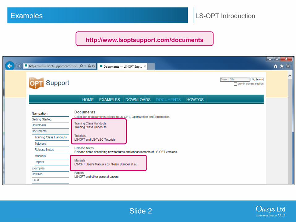
http://www.lsoptsupport.com/documents

LS-DYNA ENVIRONMENT

Introduction

LS-DYNA ENVIRONMENT

Slide 4

LS-OPT IntroductionWhat is Optimisation?

𝒙𝒙

𝒇𝒇 𝒙𝒙

𝒎𝒎𝒎𝒎𝒎𝒎 𝒇𝒇 𝒙𝒙

Infeasible design space due to design constraints

Optimisation : A procedure for achieving the best outcome of a given operation

while satisfying certain restrictions.

𝒇𝒇 𝒙𝒙𝟏𝟏,𝒙𝒙𝟐𝟐

𝒙𝒙𝟏𝟏

𝒙𝒙𝟐𝟐

LS-DYNA ENVIRONMENT

Slide 5

LS-OPT IntroductionWhat is LS-OPT?

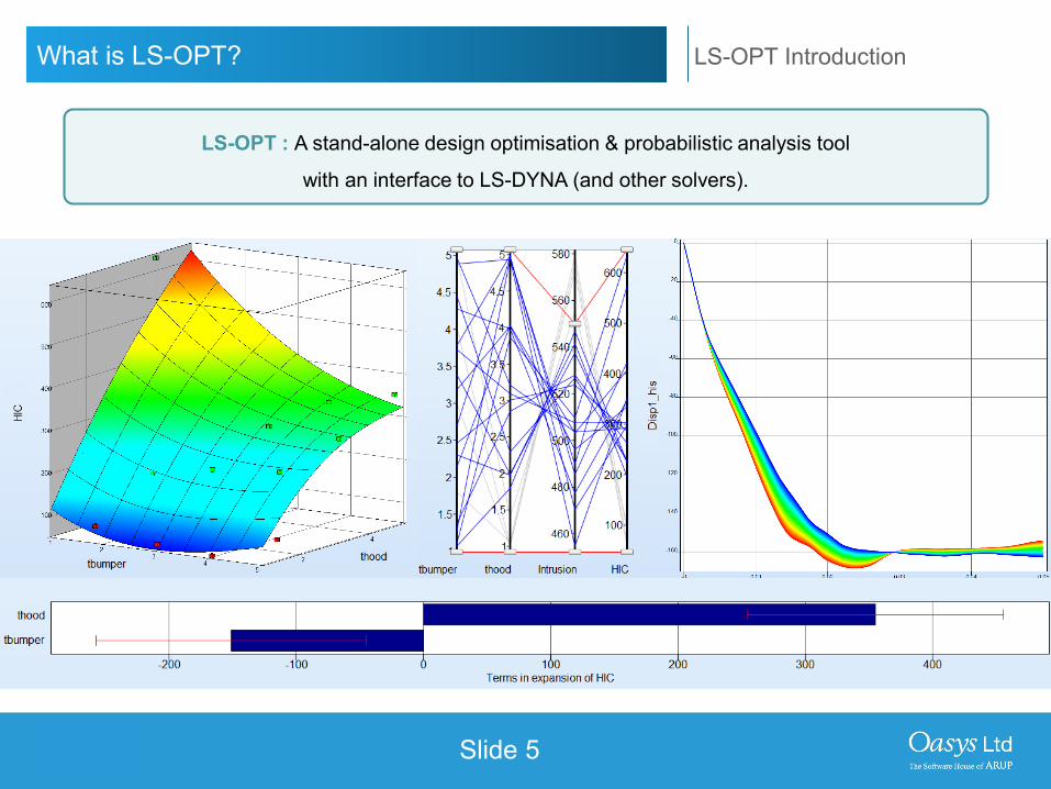
LS-OPT : A stand-alone design optimisation & probabilistic analysis tool

with an interface to LS-DYNA (and other solvers).

LS-DYNA ENVIRONMENT

Slide 6

LS-OPT IntroductionLS-OPT GUI

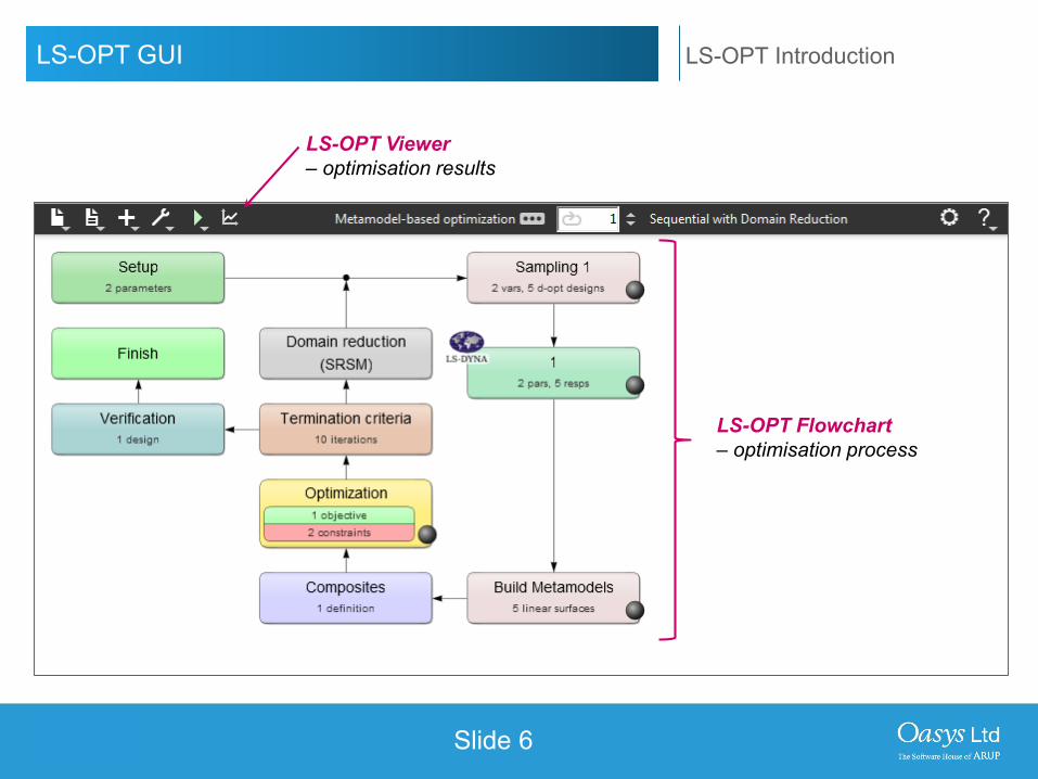
LS-OPT Viewer – optimisation results

LS-OPT Flowchart– optimisation process

LS-DYNA ENVIRONMENT

Slide 7

LS-OPT IntroductionLS-OPT Applications

Reliability based designOptimising a design with consideration of uncertainties in variables and responses.e.g. Minimising passenger injury response with respect to crush can design includingconsideration of variations in material properties and manufacturing tolerances.

Parameter identificationCalibration of a calculated curve against an input target curve.

Multi-objective optimisationOptimising a design with respect to multiple objectives.e.g. Minimising passenger injury response with respect to crush can thickness and length.

Worst-case designOptimising a design for the worst case (minimising a response with respect to somevariables while maximising the same response with respect to other variables).e.g. Minimising passenger injury response with respect to crush can design whilemaximising passenger injury response with respect to angle of impact.

NOT COVERED IN THIS WEBINAR

NOT COVERED IN THIS WEBINAR

LS-DYNA ENVIRONMENT

Design Formulation

LS-DYNA ENVIRONMENT

Slide 9

LS-OPT IntroductionDesign Formulation

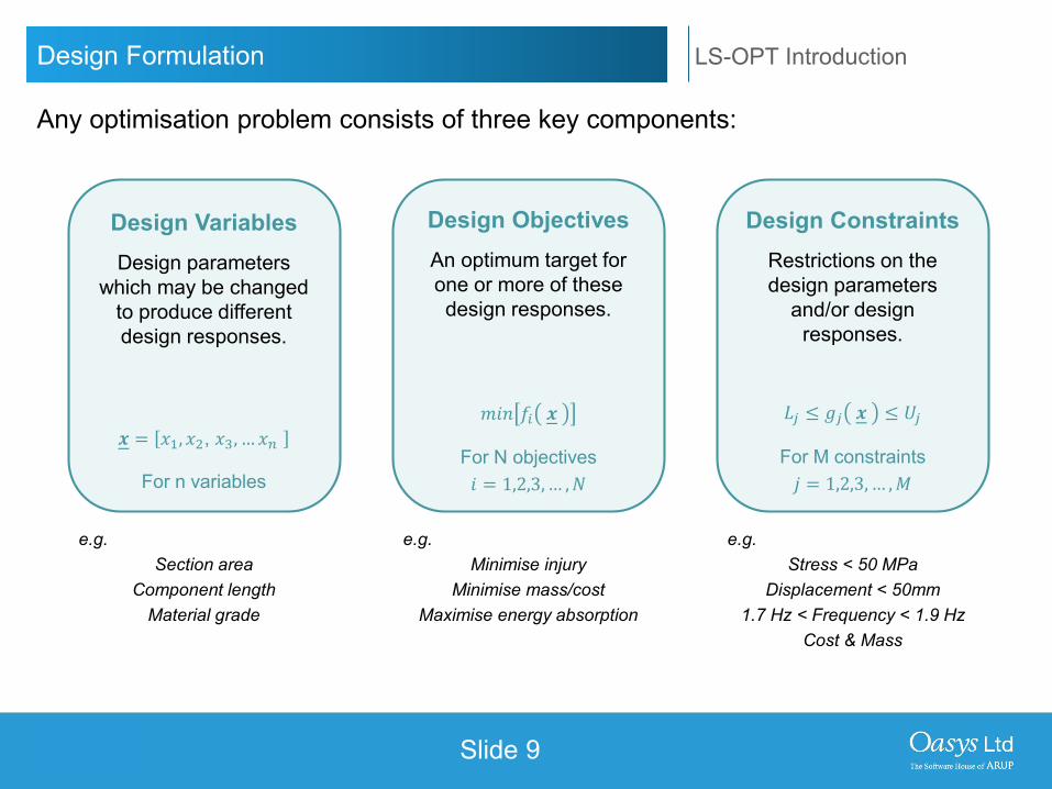
Design VariablesDesign parameters

which may be changed to produce different design responses.

𝒙𝒙 = 𝑥𝑥1,𝑥𝑥2, 𝑥𝑥3, … 𝑥𝑥𝑛𝑛

For n variables

Design ObjectivesAn optimum target for one or more of these design responses.

𝑚𝑚𝑚𝑚𝑚𝑚 𝑓𝑓𝑖𝑖 𝒙𝒙

For N objectives𝑚𝑚 = 1,2,3, … ,𝑁𝑁

Design ConstraintsRestrictions on the design parameters

and/or design responses.

𝐿𝐿𝑗𝑗 ≤ 𝑔𝑔𝑗𝑗 𝒙𝒙 ≤ 𝑈𝑈𝑗𝑗

For M constraints𝑗𝑗 = 1,2,3, … ,𝑀𝑀

e.g. Section area

Component length Material grade

e.g.Minimise injury

Minimise mass/cost Maximise energy absorption

e.g. Stress < 50 MPa

Displacement < 50mm1.7 Hz < Frequency < 1.9 Hz

Cost & Mass

Any optimisation problem consists of three key components:

LS-DYNA ENVIRONMENT

Slide 10

Responses

Variables

Composites

Objectives & constraints

1

3

4

2

LS-DYNA ENVIRONMENT

Slide 11

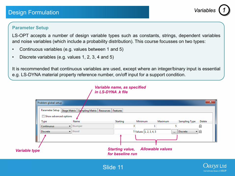
Parameter SetupLS-OPT accepts a number of design variable types such as constants, strings, dependent variablesand noise variables (which include a probability distribution). This course focusses on two types:

• Continuous variables (e.g. values between 1 and 5)

• Discrete variables (e.g. values 1, 2, 3, 4 and 5)

It is recommended that continuous variables are used, except where an integer/binary input is essentiale.g. LS-DYNA material property reference number, on/off input for a support condition.

Variable type

Variable name, as specified in LS-DYNA .k file

Allowable valuesStarting value, for baseline run

Design Formulation Variables 1

LS-DYNA ENVIRONMENT

Slide 12

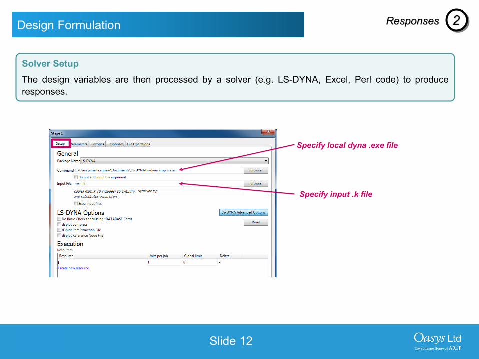
Specify input .k file

Specify local dyna .exe file

Solver SetupThe design variables are then processed by a solver (e.g. LS-DYNA, Excel, Perl code) to produceresponses.

Design Formulation Responses 2

LS-DYNA ENVIRONMENT

Slide 13

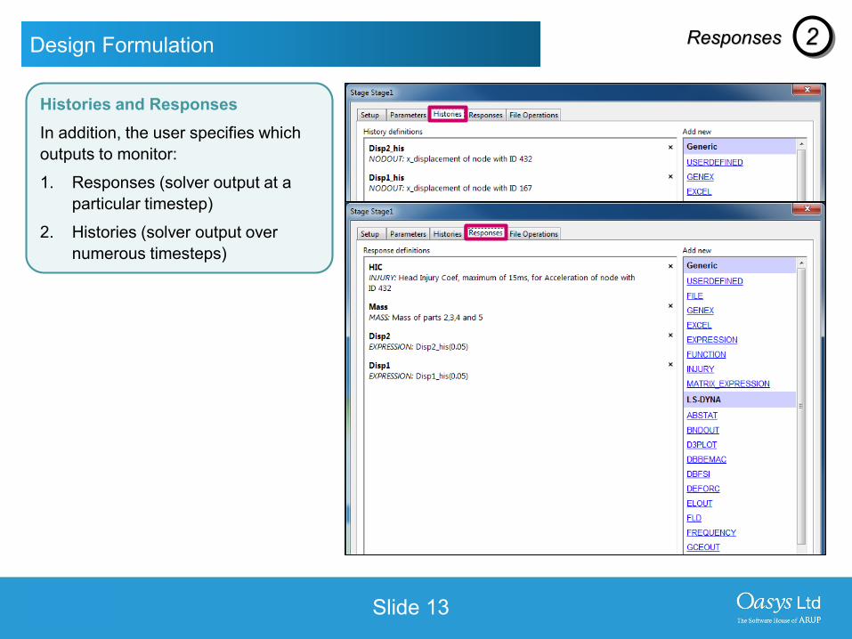
Histories and ResponsesIn addition, the user specifies which outputs to monitor:

1. Responses (solver output at a particular timestep)

2. Histories (solver output over numerous timesteps)

Design Formulation Responses 2

LS-DYNA ENVIRONMENT

Slide 14

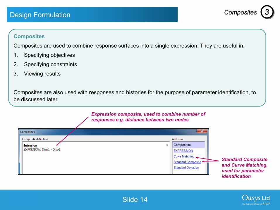
CompositesComposites are used to combine response surfaces into a single expression. They are useful in:

1. Specifying objectives

2. Specifying constraints

3. Viewing results

Composites are also used with responses and histories for the purpose of parameter identification, to be discussed later.

Expression composite, used to combine number of responses e.g. distance between two nodes

Standard Composite and Curve Matching, used for parameter identification

Design Formulation Composites 3

LS-DYNA ENVIRONMENT

Slide 15

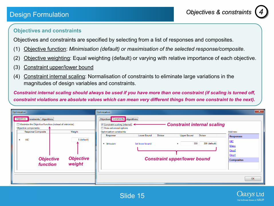
Objectives and constraintsObjectives and constraints are specified by selecting from a list of responses and composites.

(1) Objective function: Minimisation (default) or maximisation of the selected response/composite.

(2) Objective weighting: Equal weighting (default) or varying with relative importance of each objective.

(3) Constraint upper/lower bound

(4) Constraint internal scaling: Normalisation of constraints to eliminate large variations in the magnitudes of design variables and constraints.

Constraint internal scaling should always be used if you have more than one constraint (if scaling is turned off, constraint violations are absolute values which can mean very different things from one constraint to the next).

Design Formulation

Objective weight

Objective function

Constraint internal scaling

Constraint upper/lower bound

Objectives & constraints 4

LS-DYNA ENVIRONMENT

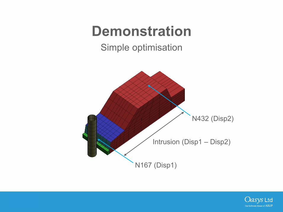
DemonstrationSimple optimisation

N432 (Disp2)

N167 (Disp1)

Intrusion (Disp1 – Disp2)

LS-DYNA ENVIRONMENT

Optimisation Methods

LS-DYNA ENVIRONMENT

Slide 18

Responses

Variables

Composites

Optimisation method

Objectives & constraints

1

3

4

2

5

LS-DYNA ENVIRONMENT

Slide 19

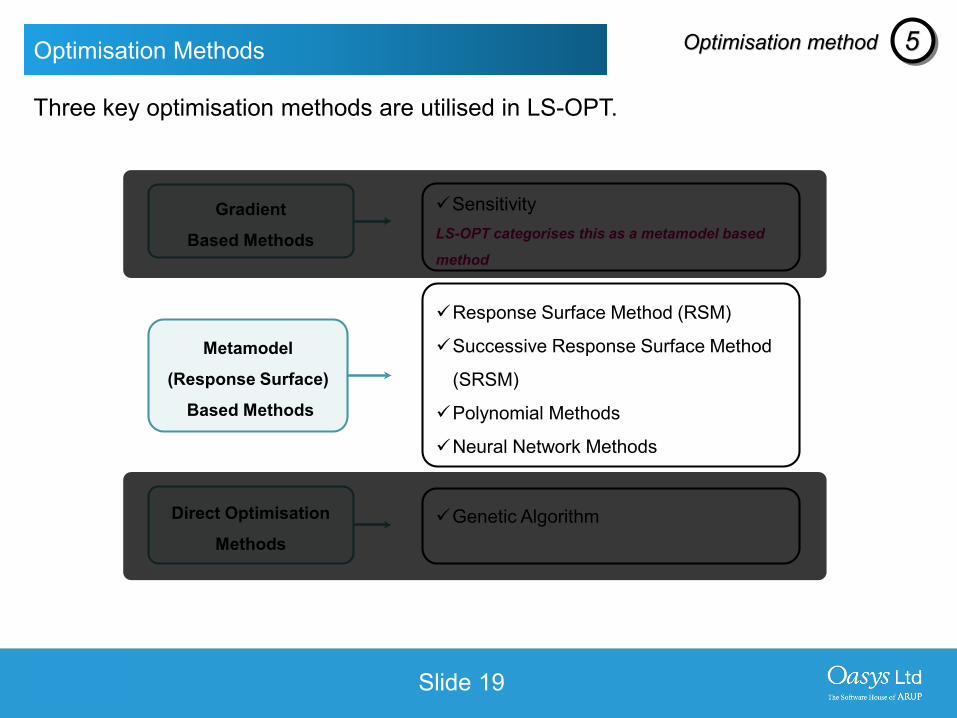
Optimisation Methods

Gradient

Based Methods

Direct Optimisation

MethodsGenetic Algorithm

Metamodel

(Response Surface)

Based Methods

Response Surface Method (RSM)

Successive Response Surface Method

(SRSM)

Polynomial Methods

Neural Network Methods

SensitivityLS-OPT categorises this as a metamodel based

method

Three key optimisation methods are utilised in LS-OPT.

Optimisation method 5

LS-DYNA ENVIRONMENT

Slide 20

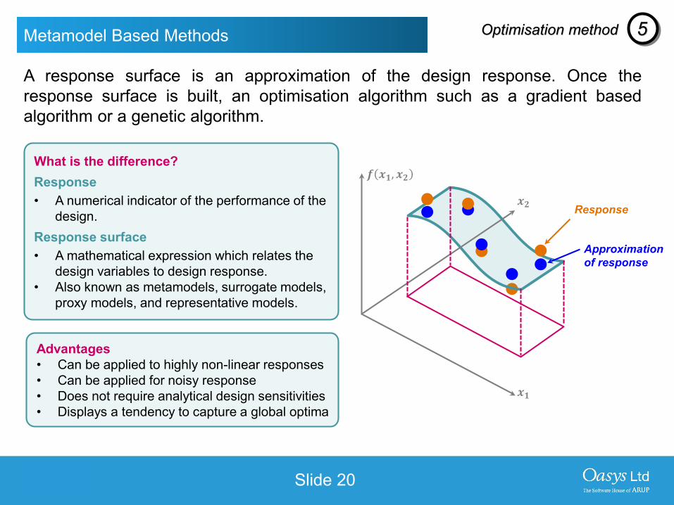
A response surface is an approximation of the design response. Once theresponse surface is built, an optimisation algorithm such as a gradient basedalgorithm or a genetic algorithm.

What is the difference?Response• A numerical indicator of the performance of the

design.Response surface• A mathematical expression which relates the

design variables to design response.• Also known as metamodels, surrogate models,

proxy models, and representative models.

Response

𝒇𝒇 𝒙𝒙𝟏𝟏,𝒙𝒙𝟐𝟐

𝒙𝒙𝟐𝟐

𝒙𝒙𝟏𝟏

Approximationof response

Advantages• Can be applied to highly non-linear responses• Can be applied for noisy response• Does not require analytical design sensitivities• Displays a tendency to capture a global optima

Gradient Based optimisationMetamodel Based Methods Optimisation method 5

LS-DYNA ENVIRONMENT

Slide 21

Metamodel Based Methods – Polynomial

Polynomial order can be linear, linear with interaction, quadratic or elliptic.

Linear Approximation

Quadratic Approximation

Optimisation method 5

LS-DYNA ENVIRONMENT

Slide 22

Metamodel Based Methods – Neural Networks

Neural networks consist of an input layer, one or more hidden layers (nodes), andan output layer, each containing a number of neurons.

𝒇𝒇

𝒇𝒇

𝒇𝒇

𝒇𝒇

Weights & biases of hidden layer

Weights & bias of output layer

Hidden Layer Output LayerInput Layer

W11

W12

W10

W1

W2

W3

W4

W0

𝑥𝑥1

𝑥𝑥2 𝑦𝑦(𝒙𝒙,𝑾𝑾)

𝒙𝒙 = (𝑥𝑥1, 𝑥𝑥2 … 𝑥𝑥𝐾𝐾)

Optimisation method 5

LS-DYNA ENVIRONMENT

Slide 23

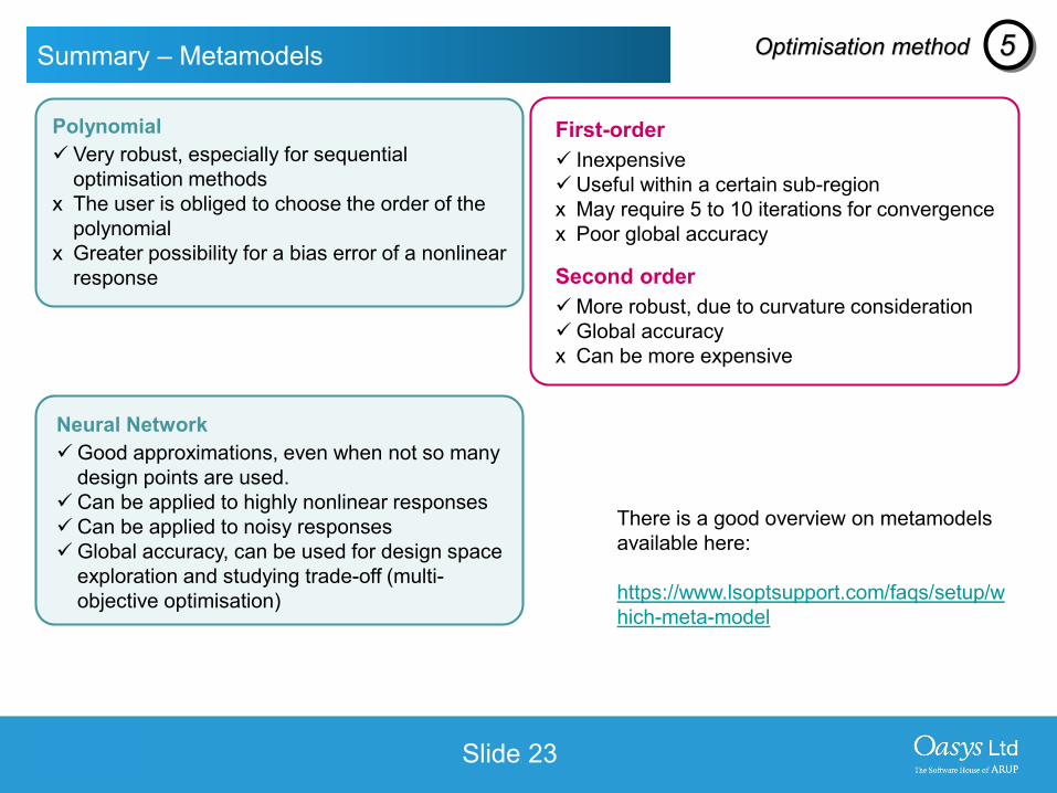
Summary – Metamodels

Polynomial Very robust, especially for sequential

optimisation methodsx The user is obliged to choose the order of the

polynomial x Greater possibility for a bias error of a nonlinear

response

Neural Network Good approximations, even when not so many

design points are used. Can be applied to highly nonlinear responses Can be applied to noisy responsesGlobal accuracy, can be used for design space

exploration and studying trade-off (multi-objective optimisation)

Optimisation method 5

First-order Inexpensive Useful within a certain sub-regionx May require 5 to 10 iterations for convergencex Poor global accuracy

Second orderMore robust, due to curvature considerationGlobal accuracyx Can be more expensive

There is a good overview on metamodels available here:

https://www.lsoptsupport.com/faqs/setup/which-meta-model

LS-DYNA ENVIRONMENT

Point Selection

LS-DYNA ENVIRONMENT

Slide 25

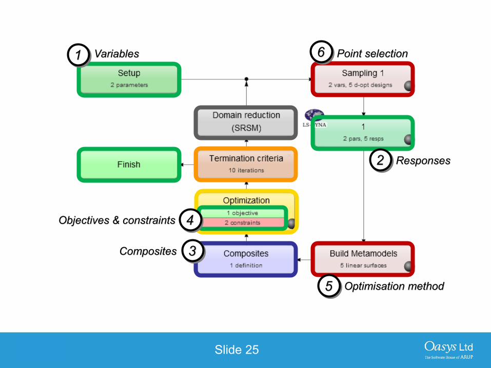
Responses

Variables

Composites

Optimisation method

Point selection

Objectives & constraints

1 6

3

4

2

5

LS-DYNA ENVIRONMENT

Slide 26

Point Selection

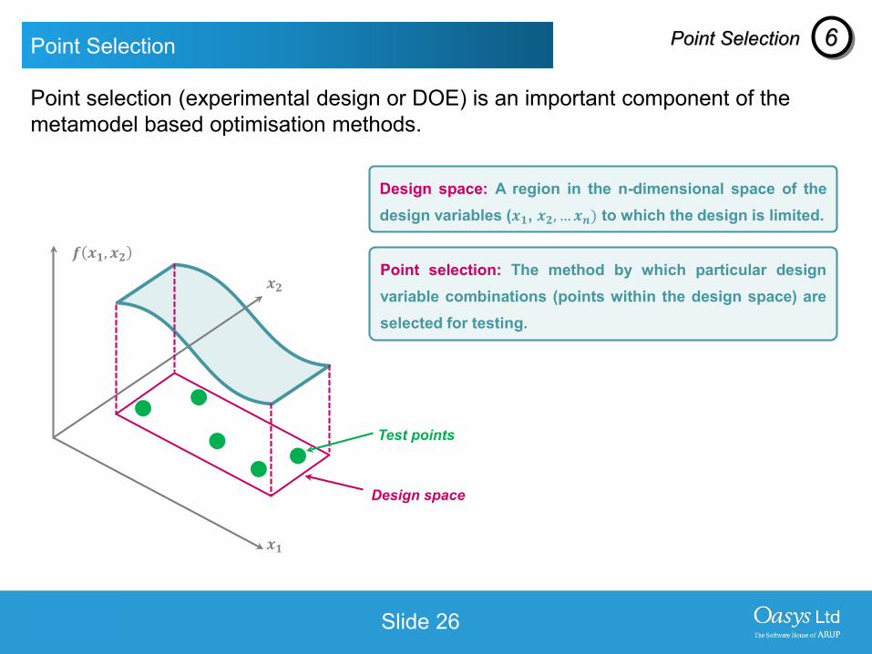
Design space: A region in the n-dimensional space of thedesign variables (𝒙𝒙𝟏𝟏, 𝒙𝒙𝟐𝟐, …𝒙𝒙𝒎𝒎) to which the design is limited.

𝒇𝒇 𝒙𝒙𝟏𝟏,𝒙𝒙𝟐𝟐

𝒙𝒙𝟐𝟐

𝒙𝒙𝟏𝟏

Test points

Design space

Point selection (experimental design or DOE) is an important component of the metamodel based optimisation methods.

Point selection: The method by which particular designvariable combinations (points within the design space) areselected for testing.

Point Selection 6

LS-DYNA ENVIRONMENT

Slide 27

Point Selection

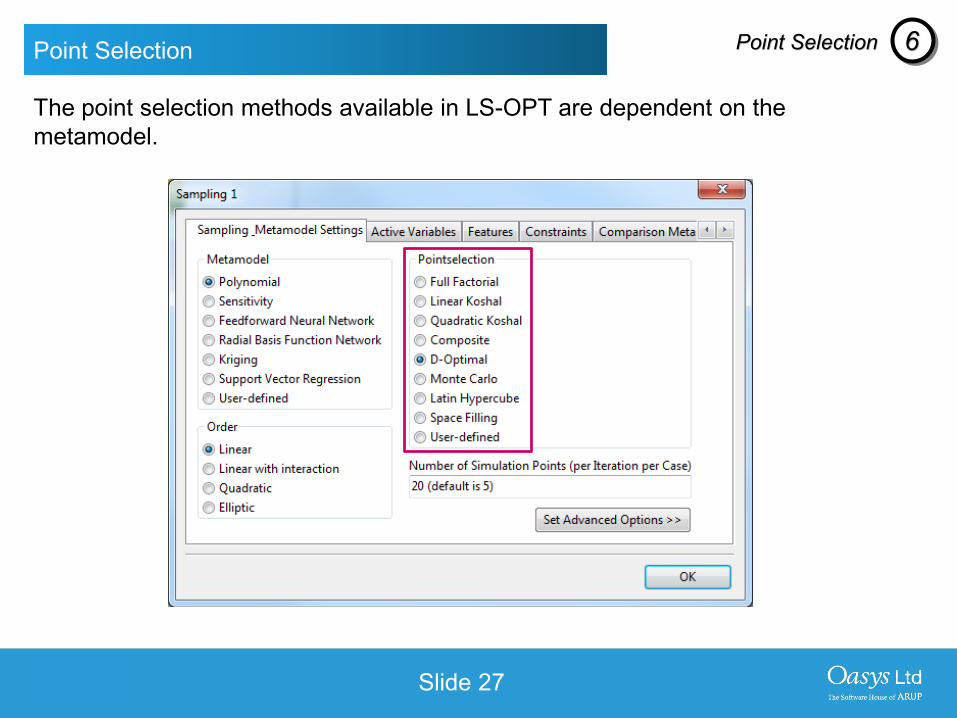
The point selection methods available in LS-OPT are dependent on the metamodel.

Point Selection 6

LS-DYNA ENVIRONMENT

Slide 28

Full Factorial

n = 2 n = 3

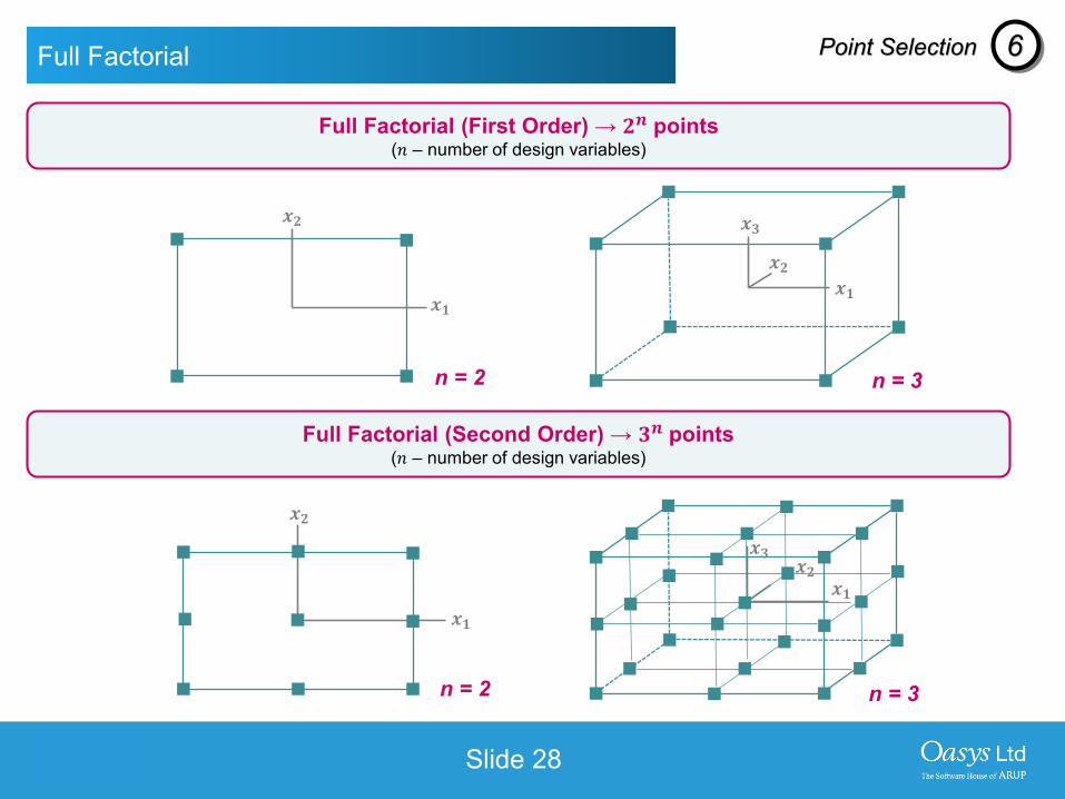
Full Factorial (First Order) → 𝟐𝟐𝒎𝒎 points(𝑚𝑚 – number of design variables)

Full Factorial (Second Order) → 𝟑𝟑𝒎𝒎 points (𝑚𝑚 – number of design variables)

n = 2 n = 3

𝒙𝒙𝟏𝟏

𝒙𝒙𝟐𝟐

𝒙𝒙𝟐𝟐

𝒙𝒙𝟏𝟏

𝒙𝒙𝟐𝟐

𝒙𝒙𝟑𝟑

𝒙𝒙𝟏𝟏

𝒙𝒙𝟐𝟐𝒙𝒙𝟑𝟑

𝒙𝒙𝟏𝟏

Point Selection 6

LS-DYNA ENVIRONMENT

Slide 29

Koshal

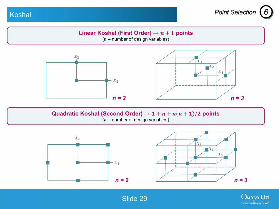
Linear Koshal (First Order) → 𝒎𝒎 + 𝟏𝟏 points (𝑚𝑚 – number of design variables)

n = 2 n = 3

n = 2 n = 3

Quadratic Koshal (Second Order) → 𝟏𝟏 + 𝒎𝒎 + 𝒎𝒎(𝒎𝒎 + 𝟏𝟏)/𝟐𝟐 points (𝑚𝑚 – number of design variables)

𝒙𝒙𝟐𝟐𝒙𝒙𝟑𝟑

𝒙𝒙𝟏𝟏

𝒙𝒙𝟐𝟐𝒙𝒙𝟑𝟑

𝒙𝒙𝟏𝟏

𝒙𝒙𝟐𝟐

𝒙𝒙𝟏𝟏

𝒙𝒙𝟐𝟐

𝒙𝒙𝟏𝟏

Point Selection 6

LS-DYNA ENVIRONMENT

Slide 30

D–Optimal

D-Optimal (Determinant optimal)

D-Optimal selects the best distribution of a specified number of design points 𝑝𝑝, by maximising the determinant 𝑿𝑿𝑇𝑇𝑿𝑿 where 𝑿𝑿is a 𝑚𝑚 x 𝑝𝑝 matrix containing all design points.

The design points are selected from a basis set, which is determined using another point selection method. The default point selection method is based on the number of variables 𝑚𝑚.• Small values of 𝑚𝑚 Full Factorial• Large values of 𝑚𝑚 Space filling

For 𝑚𝑚 > 50, Latin Hypercube is much faster.

e.g. 𝑝𝑝 = 10, 𝑚𝑚 = 2, basis set fifth order full factorial (5𝑛𝑛 points)

𝒙𝒙𝟐𝟐

𝒙𝒙𝟏𝟏

Point Selection 6

Recommended point selection for polynomial metamodels

LS-DYNA ENVIRONMENT

Slide 31

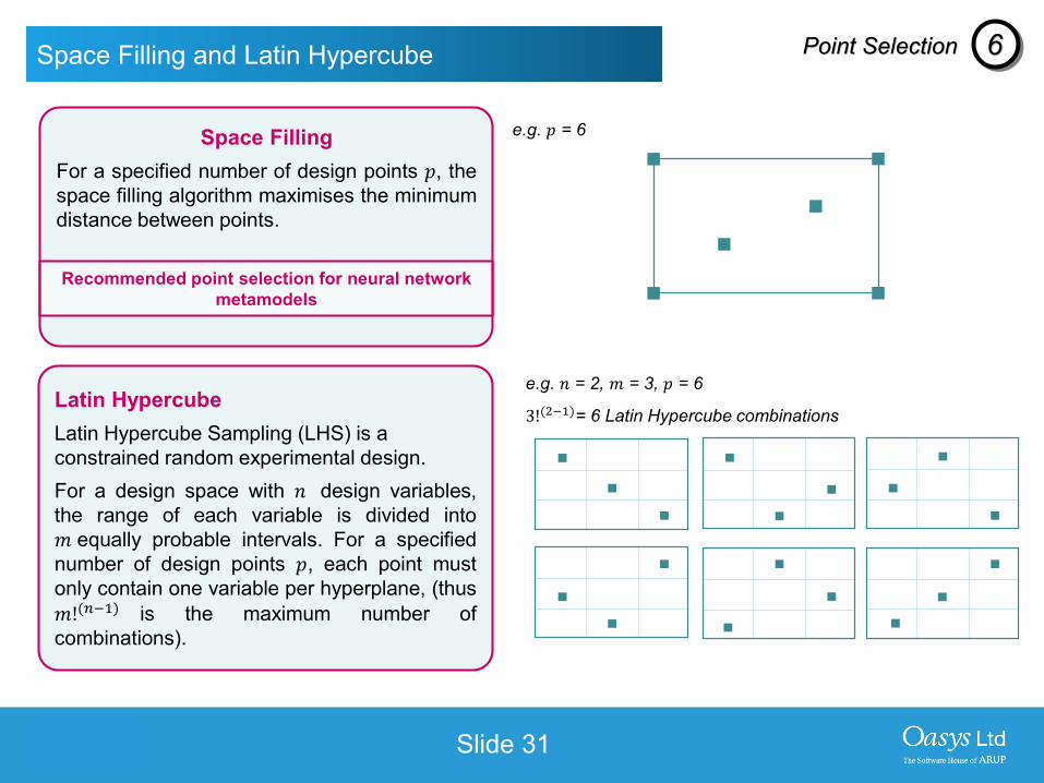
Space Filling and Latin Hypercube

Space FillingFor a specified number of design points 𝑝𝑝, thespace filling algorithm maximises the minimumdistance between points.

Latin Hypercube Latin Hypercube Sampling (LHS) is a constrained random experimental design.For a design space with 𝑚𝑚 design variables,the range of each variable is divided into𝑚𝑚 equally probable intervals. For a specifiednumber of design points 𝑝𝑝, each point mustonly contain one variable per hyperplane, (thus𝑚𝑚!(𝑛𝑛−1) is the maximum number ofcombinations).

e.g. 𝑚𝑚 = 2, 𝑚𝑚 = 3, 𝑝𝑝 = 6

3!(2−1)= 6 Latin Hypercube combinations

e.g. 𝑝𝑝 = 6

Point Selection 6

Recommended point selection for neural network metamodels

LS-DYNA ENVIRONMENT

Optimisation Strategies

LS-DYNA ENVIRONMENT

Slide 33

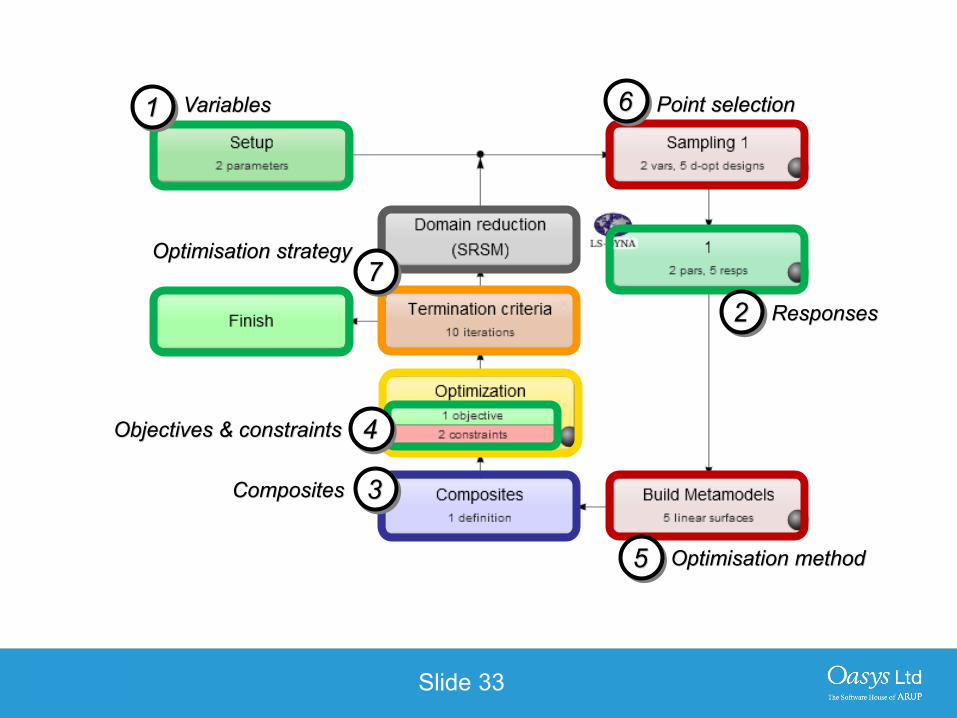
Responses

Variables

Composites

Optimisation method

Point selection

Objectives & constraints

1 6

3

4

2

5

Optimisation strategy7

LS-DYNA ENVIRONMENT

Slide 34

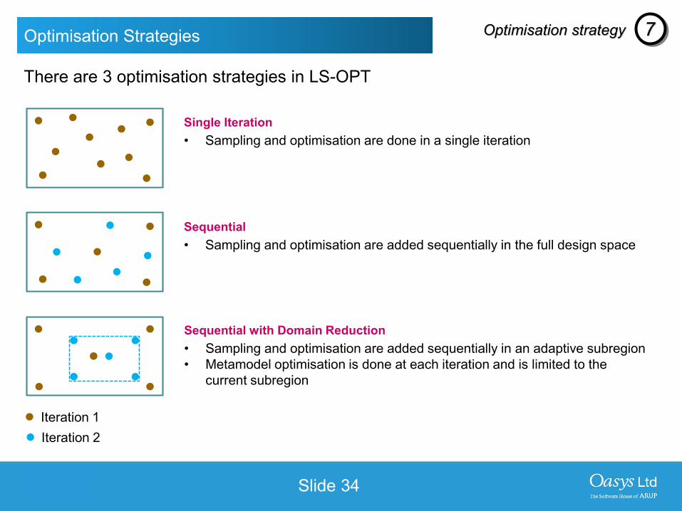
Optimisation Strategies

Single Iteration• Sampling and optimisation are done in a single iteration

Sequential• Sampling and optimisation are added sequentially in the full design space

Sequential with Domain Reduction• Sampling and optimisation are added sequentially in an adaptive subregion• Metamodel optimisation is done at each iteration and is limited to the

current subregion

There are 3 optimisation strategies in LS-OPT

Optimisation strategy 7

Iteration 1Iteration 2

LS-DYNA ENVIRONMENT

Slide 35

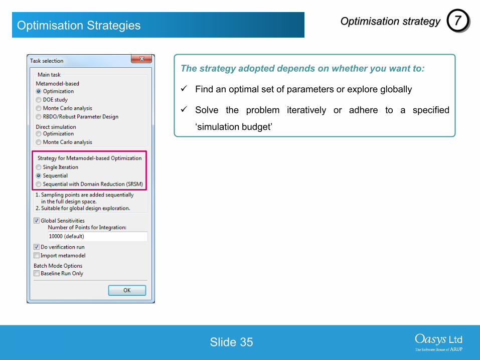
Optimisation Strategies

The strategy adopted depends on whether you want to:

Find an optimal set of parameters or explore globally

Solve the problem iteratively or adhere to a specified

‘simulation budget’

Optimisation strategy 7

LS-DYNA ENVIRONMENT

Slide 36

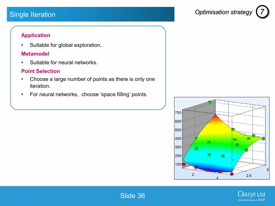
Single Iteration Optimisation strategy 7

Application

• Suitable for global exploration.Metamodel• Suitable for neural networks.Point Selection• Choose a large number of points as there is only one

iteration.• For neural networks, choose ‘space filling’ points.

LS-DYNA ENVIRONMENT

Slide 37

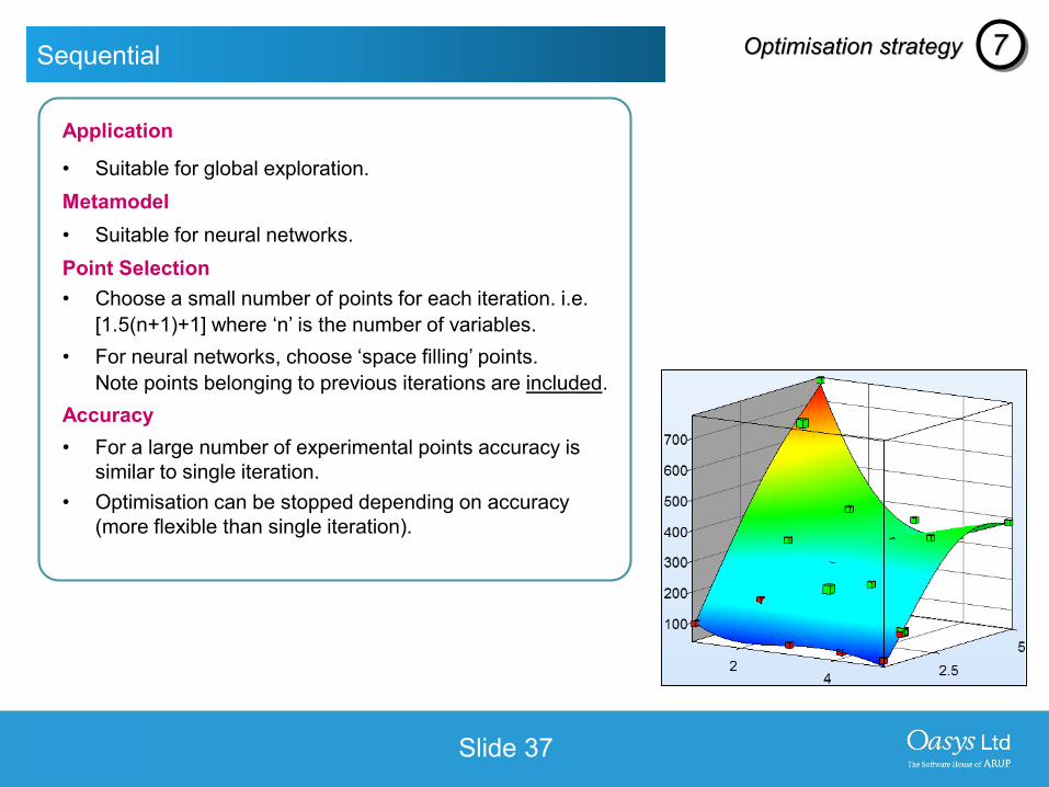
Sequential Optimisation strategy 7

Application

• Suitable for global exploration.Metamodel• Suitable for neural networks.Point Selection• Choose a small number of points for each iteration. i.e.

[1.5(n+1)+1] where ‘n’ is the number of variables.• For neural networks, choose ‘space filling’ points.

Note points belonging to previous iterations are included.Accuracy• For a large number of experimental points accuracy is

similar to single iteration.• Optimisation can be stopped depending on accuracy

(more flexible than single iteration).

LS-DYNA ENVIRONMENT

Slide 38

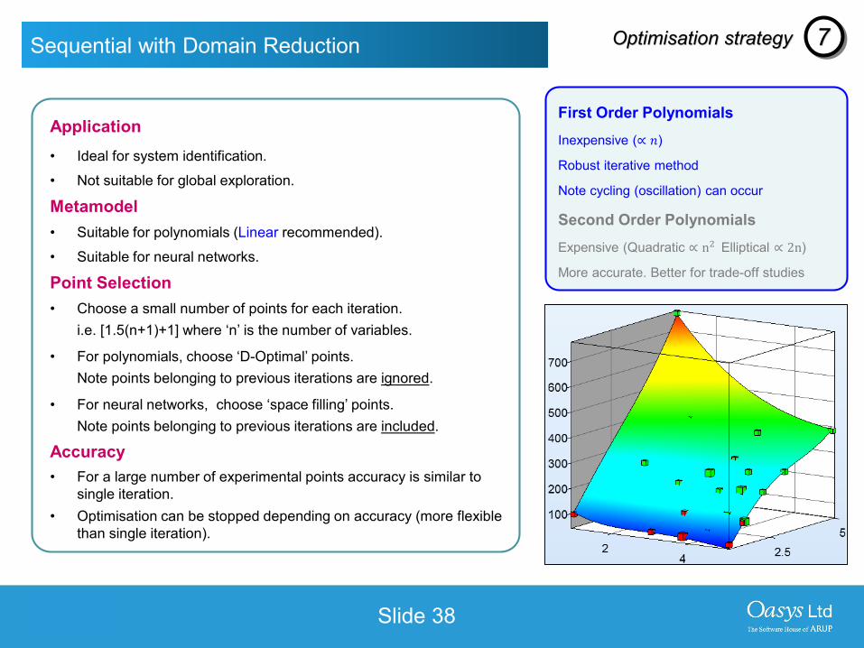
Sequential with Domain Reduction

Application• Ideal for system identification.• Not suitable for global exploration.

Metamodel• Suitable for polynomials (Linear recommended). • Suitable for neural networks.

Point Selection• Choose a small number of points for each iteration.

i.e. [1.5(n+1)+1] where ‘n’ is the number of variables.

• For polynomials, choose ‘D-Optimal’ points. Note points belonging to previous iterations are ignored.

• For neural networks, choose ‘space filling’ points. Note points belonging to previous iterations are included.

Accuracy• For a large number of experimental points accuracy is similar to

single iteration.• Optimisation can be stopped depending on accuracy (more flexible

than single iteration).

First Order PolynomialsInexpensive (∝ 𝑚𝑚)

Robust iterative method

Note cycling (oscillation) can occur

Second Order PolynomialsExpensive (Quadratic ∝ n2 Elliptical ∝ 2n)

More accurate. Better for trade-off studies

Optimisation strategy 7

LS-DYNA ENVIRONMENT

Slide 39

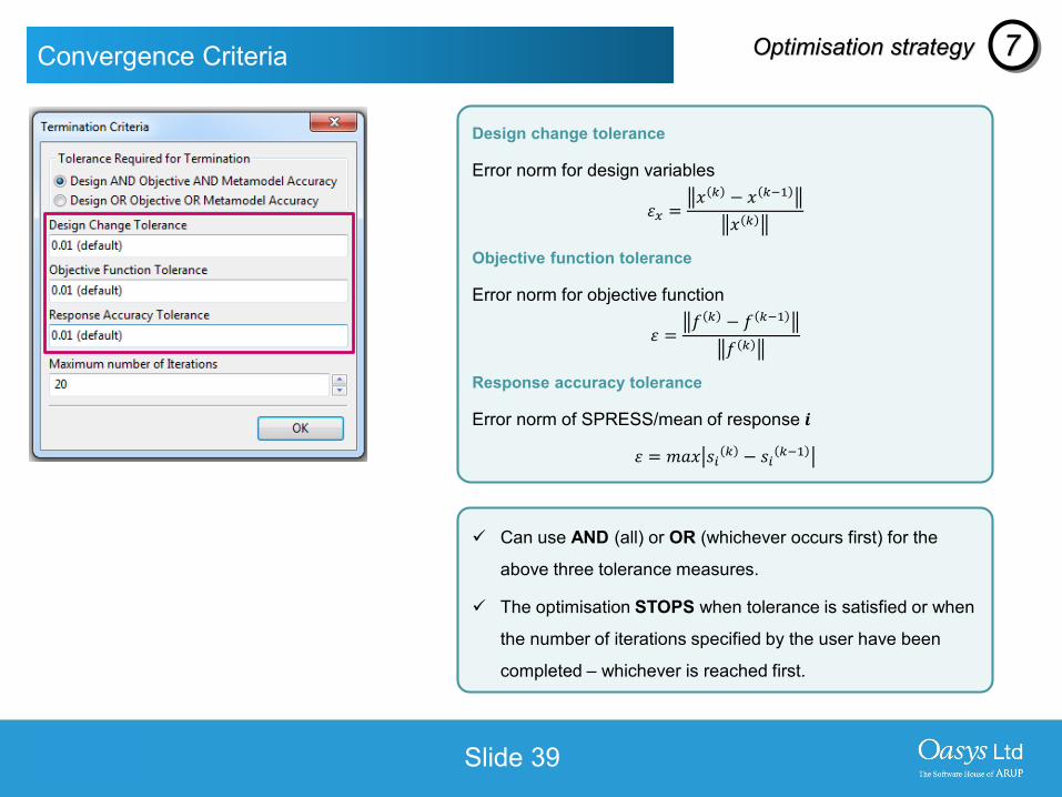
Convergence Criteria

Design change tolerance

Error norm for design variables

𝜀𝜀𝑥𝑥 =𝑥𝑥 𝑘𝑘 − 𝑥𝑥 𝑘𝑘−1

𝑥𝑥 𝑘𝑘

Objective function tolerance

Error norm for objective function

𝜀𝜀 =𝑓𝑓 𝑘𝑘 − 𝑓𝑓 𝑘𝑘−1

𝑓𝑓 𝑘𝑘

Response accuracy tolerance

Error norm of SPRESS/mean of response 𝒎𝒎

𝜀𝜀 = 𝑚𝑚𝑚𝑚𝑥𝑥 𝑠𝑠𝑖𝑖 𝑘𝑘 − 𝑠𝑠𝑖𝑖 𝑘𝑘−1

Can use AND (all) or OR (whichever occurs first) for the

above three tolerance measures.

The optimisation STOPS when tolerance is satisfied or when

the number of iterations specified by the user have been

completed – whichever is reached first.

Optimisation strategy 7

LS-DYNA ENVIRONMENT

LS-OPT Viewer

LS-DYNA ENVIRONMENT

Slide 41

LS-OPT IntroductionViewer

LS-OPT Viewer offers a number of graphical plot options to view the results.We will now take a look at some key plots.

Simulations Focuses on the computed data (e.g. LS-DYNA results)

MetamodelFocuses on the metamodel predicted data

OptimisationFocuses on the genetic algorithm or metamodel predicted data over a number of iterations

LS-DYNA ENVIRONMENT

Slide 42

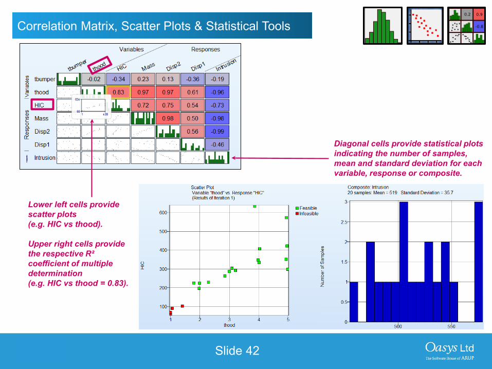
Correlation Matrix, Scatter Plots & Statistical Tools

Lower left cells provide scatter plots (e.g. HIC vs thood).

Upper right cells provide the respective R² coefficient of multiple determination(e.g. HIC vs thood = 0.83).

Diagonal cells provide statistical plots indicating the number of samples, mean and standard deviation for each variable, response or composite.

LS-DYNA ENVIRONMENT

Slide 43

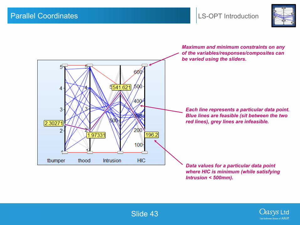
LS-OPT IntroductionParallel Coordinates

Data values for a particular data point where HIC is minimum (while satisfying Intrusion < 500mm).

Maximum and minimum constraints on any of the variables/responses/composites can be varied using the sliders.

Each line represents a particular data point. Blue lines are feasible (sit between the two red lines), grey lines are infeasible.

LS-DYNA ENVIRONMENT

Slide 44

LS-OPT IntroductionSurface

Computed data points may also be plotted, with feasible points coloured green, and infeasible points coloured red.

Surface plot allows us to view the response surface in 3D.

LS-DYNA ENVIRONMENT

Slide 45

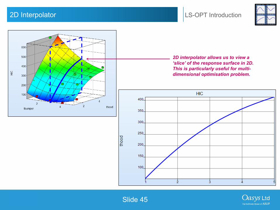
LS-OPT Introduction2D Interpolator

2D interpolator allows us to view a ‘slice’ of the response surface in 2D.This is particularly useful for multi-dimensional optimisation problem.

LS-DYNA ENVIRONMENT

Sensitivity Analysis

LS-DYNA ENVIRONMENT

Slide 47

LS-OPT IntroductionSensitivity Analysis

Sensitivity Analysis

Sensitivity analysis allows the user to identify and remove variables which have insignificant contributions to the metamodel. Reduce number of variables. Reduce computational effort.

There are two sensitivity analysis tools in LS-OPT:• Analysis of Variance (ANOVA)• Global Sensitivity Analysis (GSA)

LS-DYNA ENVIRONMENT

Slide 48

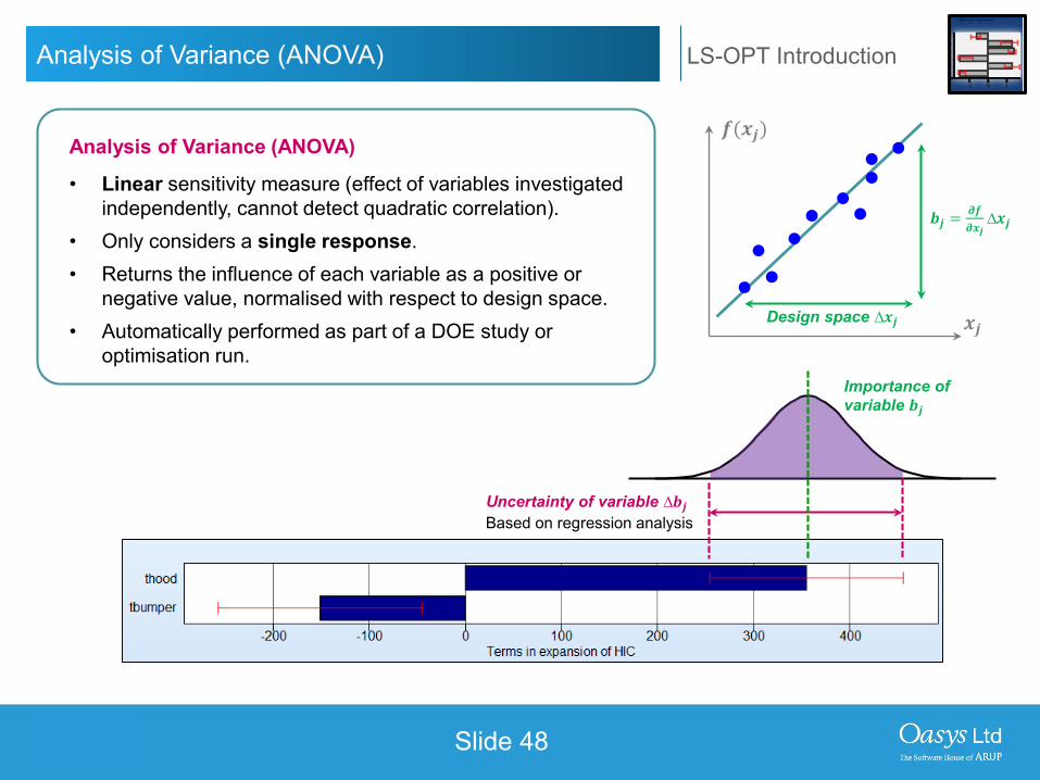
LS-OPT IntroductionAnalysis of Variance (ANOVA)

Uncertainty of variable ∆𝒃𝒃𝒋𝒋Based on regression analysis

Analysis of Variance (ANOVA)

• Linear sensitivity measure (effect of variables investigated independently, cannot detect quadratic correlation).

• Only considers a single response.• Returns the influence of each variable as a positive or

negative value, normalised with respect to design space.• Automatically performed as part of a DOE study or

optimisation run.Importance of variable 𝒃𝒃𝒋𝒋

𝒃𝒃𝒋𝒋 = 𝝏𝝏𝒇𝒇𝝏𝝏𝒙𝒙𝒋𝒋

∆𝒙𝒙𝒋𝒋

Design space ∆𝒙𝒙𝒋𝒋 𝒙𝒙𝒋𝒋

𝒇𝒇(𝒙𝒙𝒋𝒋)

LS-DYNA ENVIRONMENT

Slide 49

LS-OPT IntroductionGlobal Sensitivity Analysis (GSA)

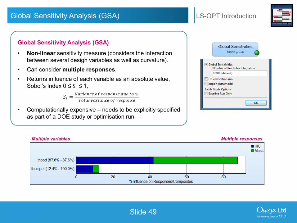
Global Sensitivity Analysis (GSA)

• Non-linear sensitivity measure (considers the interaction between several design variables as well as curvature).

• Can consider multiple responses. • Returns influence of each variable as an absolute value,

Sobol’s Index 0 ≤ Si ≤ 1,

𝑆𝑆𝑖𝑖 = 𝑉𝑉𝑉𝑉𝑉𝑉𝑖𝑖𝑉𝑉𝑛𝑛𝑉𝑉𝑉𝑉 𝑜𝑜𝑜𝑜 𝑉𝑉𝑉𝑉𝑟𝑟𝑟𝑟𝑜𝑜𝑛𝑛𝑟𝑟𝑉𝑉 𝑑𝑑𝑑𝑑𝑉𝑉 𝑡𝑡𝑜𝑜 𝑥𝑥𝑖𝑖𝑇𝑇𝑜𝑜𝑡𝑡𝑉𝑉𝑜𝑜 𝑣𝑣𝑉𝑉𝑉𝑉𝑖𝑖𝑉𝑉𝑛𝑛𝑉𝑉𝑉𝑉 𝑜𝑜𝑜𝑜 𝑉𝑉𝑉𝑉𝑟𝑟𝑟𝑟𝑜𝑜𝑛𝑛𝑟𝑟𝑉𝑉

• Computationally expensive – needs to be explicitly specified as part of a DOE study or optimisation run.

Multiple variables Multiple responses

LS-DYNA ENVIRONMENT

Slide 50

LS-OPT IntroductionInterpreting ANOVA & GSA

The ANOVA and GSA should be considered in parallel.

ANOVA• The error bars represent the contribution of the variables to noise or poorness of fit in a

linear approximation of the computed responses.• The bar lengths represent the influence of the variables on the linear approximation.• The bar directions represents whether the variables have a positive or negative influence on

the linear approximation.

GSA• The bar lengths represent the influence of the variables on the response surface, as a

percentage of the total variance of the response surface.• The total variation value (provided at the top of the GSA plot) indicates this total variance.• The noise variation value (also provided at the top of the GSA plot) indicates the noise or

poorness of fit of the response surface to the computed responses.

LS-DYNA ENVIRONMENT

Slide 51

LS-OPT IntroductionExample 1

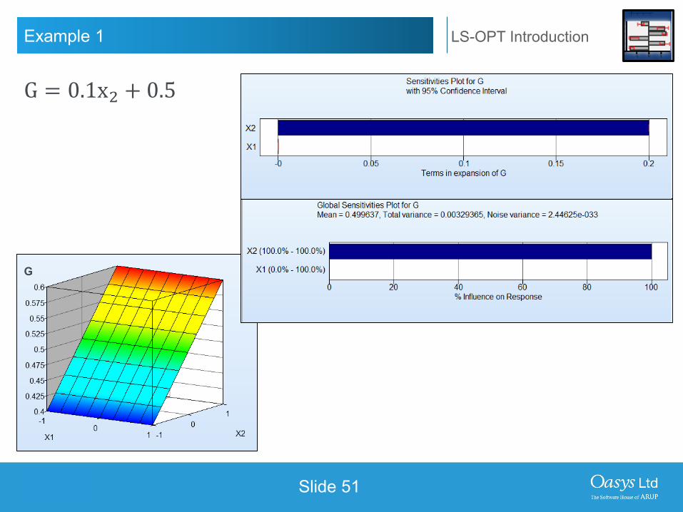
G

G = 0.1x2 + 0.5

LS-DYNA ENVIRONMENT

Slide 52

LS-OPT IntroductionExample 2

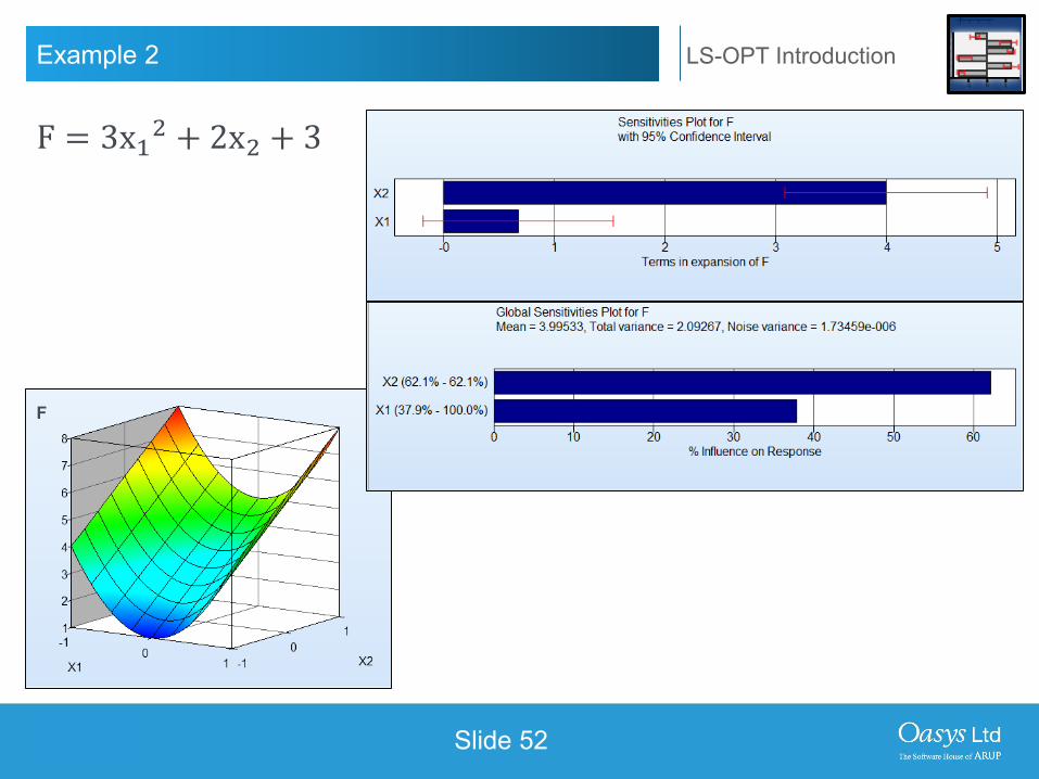
F

F = 3x12 + 2x2 + 3

LS-DYNA ENVIRONMENT

Error Analysis

LS-DYNA ENVIRONMENT

Slide 54

LS-OPT IntroductionError Analysis

Random error

Modeling error

Response Surface𝒙𝒙

𝒇𝒇 𝒙𝒙

Response

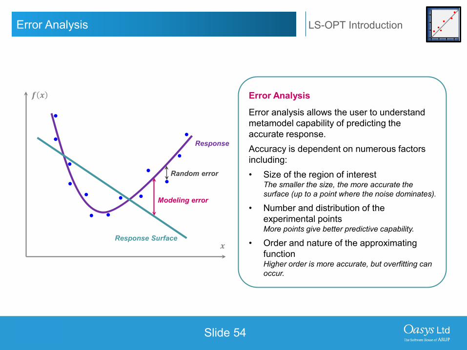
Error Analysis

Error analysis allows the user to understand metamodel capability of predicting the accurate response.Accuracy is dependent on numerous factors including:• Size of the region of interest

The smaller the size, the more accurate the surface (up to a point where the noise dominates).

• Number and distribution of the experimental points More points give better predictive capability.

• Order and nature of the approximating function Higher order is more accurate, but overfitting can occur.

LS-DYNA ENVIRONMENT

Slide 55

LS-OPT IntroductionError Analysis

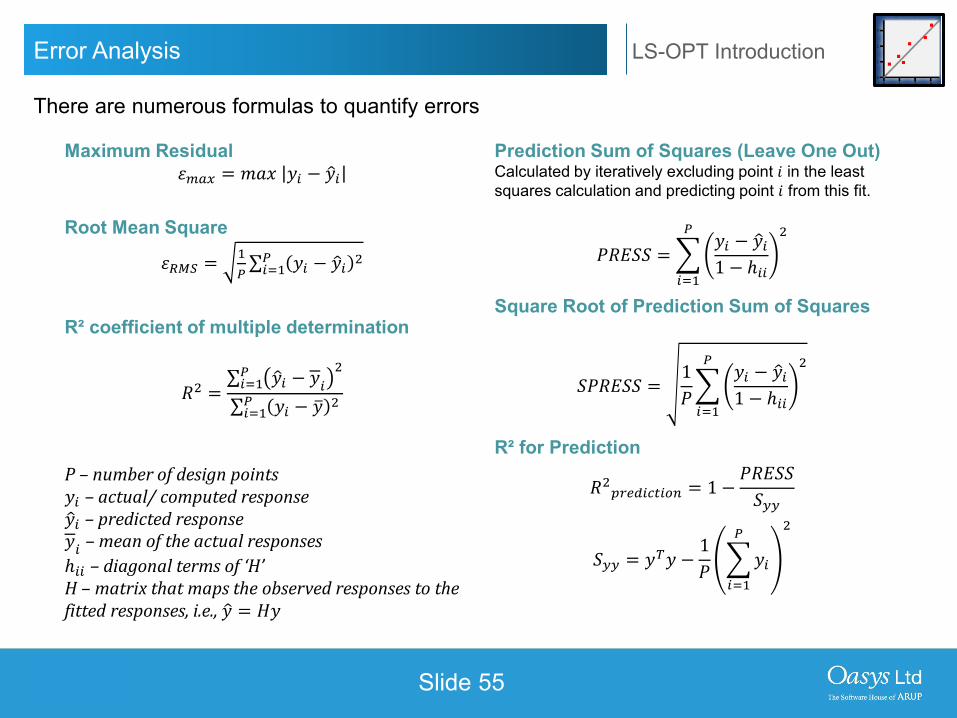
Maximum Residual𝜀𝜀𝑚𝑚𝑉𝑉𝑥𝑥 = 𝑚𝑚𝑚𝑚𝑥𝑥 𝑦𝑦𝑖𝑖 − �𝑦𝑦𝑖𝑖

Root Mean Square

𝜀𝜀𝑅𝑅𝑅𝑅𝑅𝑅 = 1𝑃𝑃∑𝑖𝑖=1𝑃𝑃 𝑦𝑦𝑖𝑖 − �𝑦𝑦𝑖𝑖 2

R² coefficient of multiple determination

𝑅𝑅2 =∑𝑖𝑖=1𝑃𝑃 �𝑦𝑦𝑖𝑖 − 𝑦𝑦𝑖𝑖

2

∑𝑖𝑖=1𝑃𝑃 𝑦𝑦𝑖𝑖 − �𝑦𝑦 2

P – number of design points𝑦𝑦𝑖𝑖 – actual/ computed response�𝑦𝑦𝑖𝑖 – predicted response𝑦𝑦𝑖𝑖 – mean of the actual responsesℎ𝑖𝑖𝑖𝑖 – diagonal terms of ‘H’H – matrix that maps the observed responses to the fitted responses, i.e., �𝑦𝑦 = 𝐻𝐻𝑦𝑦

Prediction Sum of Squares (Leave One Out)Calculated by iteratively excluding point 𝑚𝑚 in the least squares calculation and predicting point 𝑚𝑚 from this fit.

𝑃𝑃𝑅𝑅𝑃𝑃𝑆𝑆𝑆𝑆 = �𝑖𝑖=1

𝑃𝑃𝑦𝑦𝑖𝑖 − �𝑦𝑦𝑖𝑖1 − ℎ𝑖𝑖𝑖𝑖

2

Square Root of Prediction Sum of Squares

𝑆𝑆𝑃𝑃𝑅𝑅𝑃𝑃𝑆𝑆𝑆𝑆 =1𝑃𝑃�𝑖𝑖=1

𝑃𝑃𝑦𝑦𝑖𝑖 − �𝑦𝑦𝑖𝑖1 − ℎ𝑖𝑖𝑖𝑖

2

R² for Prediction

𝑅𝑅2𝑟𝑟𝑉𝑉𝑉𝑉𝑑𝑑𝑖𝑖𝑉𝑉𝑡𝑡𝑖𝑖𝑜𝑜𝑛𝑛 = 1 −𝑃𝑃𝑅𝑅𝑃𝑃𝑆𝑆𝑆𝑆𝑆𝑆𝑦𝑦𝑦𝑦

𝑆𝑆𝑦𝑦𝑦𝑦 = 𝑦𝑦𝑇𝑇𝑦𝑦 −1𝑃𝑃 �

𝑖𝑖=1

𝑃𝑃

𝑦𝑦𝑖𝑖

2

There are numerous formulas to quantify errors

LS-DYNA ENVIRONMENT

Slide 56

LS-OPT IntroductionExample 1

LS-DYNA ENVIRONMENT

Slide 57

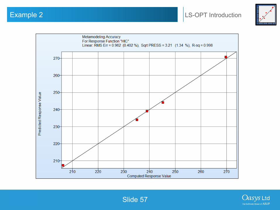
LS-OPT IntroductionExample 2

LS-DYNA ENVIRONMENT

Multi-Objective Optimisation

LS-DYNA ENVIRONMENT

Slide 59

LS-OPT IntroductionMulti-Objective Optimisation

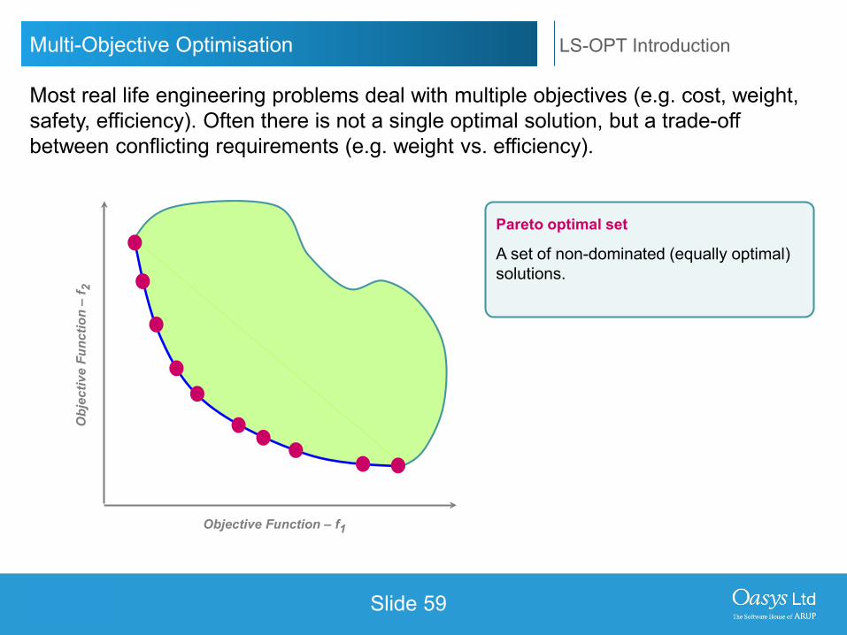
Most real life engineering problems deal with multiple objectives (e.g. cost, weight, safety, efficiency). Often there is not a single optimal solution, but a trade-off between conflicting requirements (e.g. weight vs. efficiency).

Pareto optimal set

A set of non-dominated (equally optimal) solutions.

Obj

ectiv

e Fu

nctio

n –

f 2

Objective Function – f1

LS-DYNA ENVIRONMENT

Slide 60

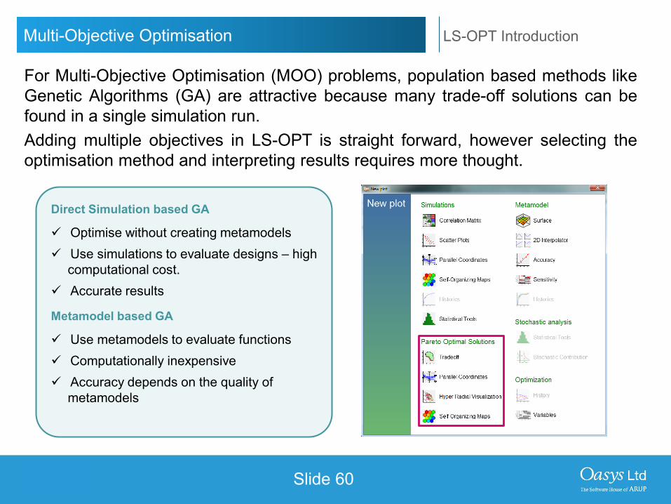
LS-OPT IntroductionMulti-Objective Optimisation

Direct Simulation based GA

Optimise without creating metamodels Use simulations to evaluate designs – high

computational cost. Accurate results

Metamodel based GA

Use metamodels to evaluate functions Computationally inexpensive Accuracy depends on the quality of

metamodels

For Multi-Objective Optimisation (MOO) problems, population based methods likeGenetic Algorithms (GA) are attractive because many trade-off solutions can befound in a single simulation run.Adding multiple objectives in LS-OPT is straight forward, however selecting theoptimisation method and interpreting results requires more thought.

LS-DYNA ENVIRONMENT

Slide 61

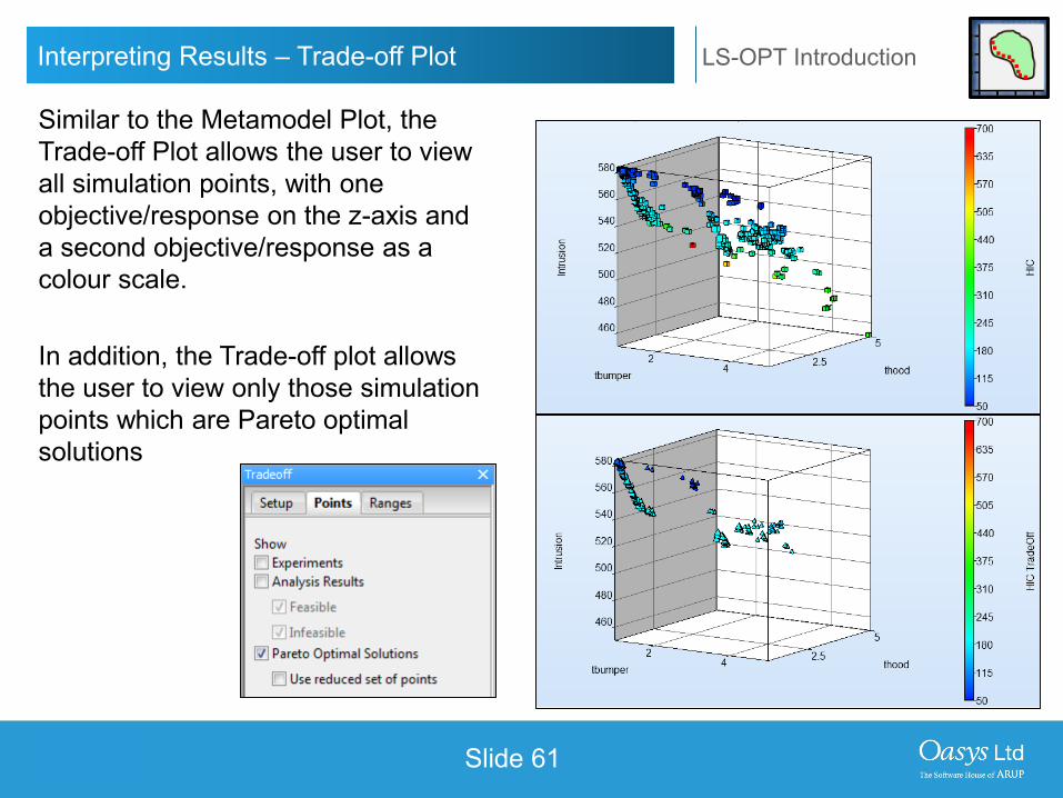
LS-OPT IntroductionInterpreting Results – Trade-off Plot

Similar to the Metamodel Plot, the Trade-off Plot allows the user to view all simulation points, with one objective/response on the z-axis and a second objective/response as a colour scale.

In addition, the Trade-off plot allows the user to view only those simulation points which are Pareto optimal solutions

LS-DYNA ENVIRONMENT

Parameter Identification

LS-DYNA ENVIRONMENT

Slide 63

LS-OPT IntroductionParameter Identification

Parameter identification is based on minimising the mismatch between targetvalues and solver-computed outputs.

LS-OPT Parameter Identification

Parameter Identification MethodsThere are two key parameter identification methods available in LS-OPT1. MSE or Ordinate Based Curve Matching

(Point based or History based)2. Curve Mapping

(History based)

Optimisation Settings The following optimisation settings are recommended:• Linear polynomial metamodel • D-optimal point selection• Sequential domain reduction

Computed Curve

Target Curve

LS-DYNA ENVIRONMENT

Slide 64

LS-OPT IntroductionParameter Identification

Ordinate based curve matching Optimisation is based on the Mean Squared Error (MSE) metric which calculates the discrepancy in ordinate values between two curves.

𝑀𝑀𝑆𝑆𝑃𝑃 =1𝑃𝑃�𝑟𝑟=1

𝑃𝑃

𝑊𝑊𝑟𝑟𝑓𝑓𝑟𝑟 𝒙𝒙 − 𝐺𝐺𝑟𝑟

𝑆𝑆𝑟𝑟

2

ApplicationOrdinate based curve matching is used for non-steep curves with unique abscissa values only.• Steep portions of the response are

difficult or impossible to incorporate (e.g. linear elastic range or failure).

• Hysteretic test curves cannot be matched since the abscissa values are non-monotonic/non-unique.

• Results in instability if ranges of the computed and test curve do not coincide in the y-axis (ordinate) at an interim stage of the optimisation.

• Partial matching is not robust.

𝑃𝑃 is the number of points, 𝑆𝑆𝑟𝑟 is the residual scale factor (normalisation of error), and 𝑊𝑊𝑟𝑟 is the weight factor

Computed Curve 𝒇𝒇 𝒙𝒙, 𝒛𝒛 Target Curve

𝑮𝑮 𝒛𝒛

𝒇𝒇 𝒙𝒙, 𝒛𝒛 ,𝑮𝑮 𝒛𝒛

Residual

𝒛𝒛

LS-DYNA ENVIRONMENT

Slide 65

LS-OPT IntroductionSetup – History Based Parameter Identification

1. Set up a history definition for the computed curve.

2. Create a curve matching composite. – Set algorithm to MSE (shown) or

Curve Mapping.– Specify the target curve in a history

file and import. – Specify the computed curve.

3. Define the composite as an objective function.

4. Run optimisation.

LS-DYNA ENVIRONMENT

Slide 66

LS-OPT IntroductionInterpreting Results

Parameter identification results are often best viewed using History Plots. By displaying only the optimum solution for each iteration, and colouring the curves by iteration, we can clearly see the curves converge on the input data points.

Target (input) data history

Computed data history

LS-DYNA ENVIRONMENT

Slide 67

LS-OPT IntroductionInterpreting Results

The calculated parameter values, and the convergence of the optimisation to these values can be viewed as an optimisation History Plot.

Reduction in domain

Converged solution

LS-DYNA ENVIRONMENT

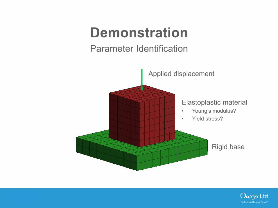
DemonstrationParameter Identification

Elastoplastic material• Young’s modulus?• Yield stress?

Applied displacement

Rigid base

LS-DYNA ENVIRONMENT

Conclusion

LS-DYNA ENVIRONMENT

Slide 70

LS-OPT Introduction

2. Design Formulation3. Optimisation Methods4. Point Selection5. Optimisation Strategy

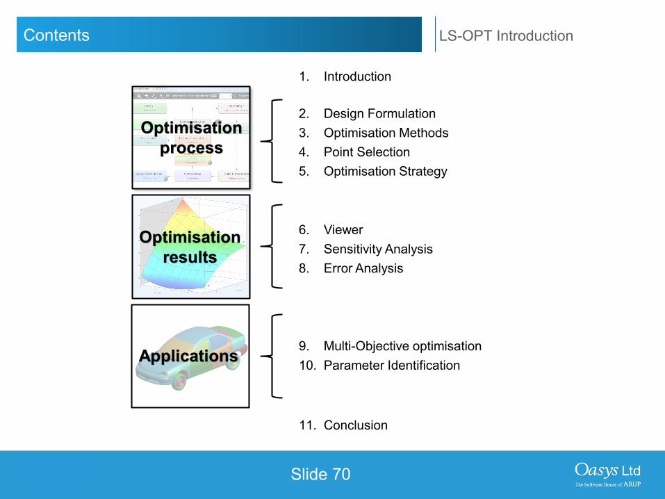
Contents

Optimisation process

Optimisation results

Applications

6. Viewer7. Sensitivity Analysis8. Error Analysis

1. Introduction

11. Conclusion

9. Multi-Objective optimisation10. Parameter Identification

LS-DYNA ENVIRONMENT

Slide 71

LS-OPT IntroductionGlossary

• ANOVA – Analysis of Variance• ASA – Adaptive Simulated Annealing• DOE – Design of Experiments• FFNN – Feed Forward Neural Network• GA – Genetic Algorithm• GSA – Global Sensitivity Analysis• GUI – Graphical User Interface• LFOP – Leap-Frog Optimiser• LHS – Latin Hypercube Sampling• MOO – Multi-Objective Optimisation• MSE – Mean Square Error• NN – Neural Network• PRESS – Prediction Sum of Squares• RBF – Radial Basis Function• RMS – Root Mean Square• RSM – Response Surface Method• SRSM – Successive Response Surface Method

LS-DYNA ENVIRONMENT

Slide 72

LS-OPT IntroductionContact Information

For more information please contact the following:

www.arup.com/dyna

UK Contact:The Arup CampusBlythe Valley ParkSolihullB90 8AEUnited Kingdom

T +44 (0)121 213 3399dyna.support@arup.com

China Contact:Arup China39/F-41/F Huaihai Plaza 1045 Huaihai Road (M)Xuhui District, Shanghai200031China

T +86 21 6126 2875china.support@arup.com

India ContactArup IndiaAnanth Info Park, HiTec City Madhapur Phase-IIHyderabad500 081, TelanganaIndia

T +91 (0) 40 44369797 / 8 india.support@arup.com

USA West ContactArup Americasc/o 560 Mission Street Suite 700San FranciscoCA 94105United States

T +1 415 940 0959 us.support@arup.com