Love, Money, and Parental Goods:

Does Parental Matchmaking Matter?∗

Fali Huanga, Ginger Zhe Jinb, Lixin Colin Xuc

August 2, 2016

a School of Economics, Singapore Management University, 90 Stamford Road, Singapore 178903, �huang@smu.edu.sg. b

Department of Economics, University of Maryland & NBER, College Park, MD 20742, jin@econ.umd.edu. c World Bank 1818

H Street, N.W. Washington, D.C., 20433, lxu1@worldbank.org. Tel : +1 202 473 4664. Corresponding author.

Abstract

While parental matchmaking has been widespread throughout history and across

countries, we know little about the relationship between parental matchmaking and

marriage outcomes. Does parental involvement in matchmaking help ensure their needs

are better taken care of by married children? This paper �nds supportive evidence

using a survey of Chinese couples. In particular, parental involvement in matchmaking

is associated with having a more submissive wife, a greater number of children, a

higher likelihood of having any male children, and a stronger belief of the husband in

providing old age support to his parents. These bene�ts, however, are achieved at the

cost of less marital harmony within the couple and lower market income of the wife.

The results render support to and extend the �ndings of Becker, Murphy and Spenkuch

(2015) where parents meddle with children's preferences to ensure their commitment

to providing parental goods such as old age support.

∗We wish to thank Yuyu Chen, Steve Cheung, William Evans, James Heckman, Bert Ho�man, Yi Lu,Vijayendra Rao, Seth Sanders, Mary Shirley, Je�rey Smith, Liming Wang, Dali Yang, and participants atthe Chicago-Renmin symposium on family and labor economics at the University of Chicago, the symposiumof the 80th birthday of Steven Cheung at Shenzhen, U. of Maryland workshop, the AEA meetings, the PAAconference, and the Asian Conference on Applied Micro-Economics/Econometrics at Tokyo for constructivecomment and suggestions. We are especially grateful to the late Gary Becker for his detailed comments atthe Chicago-Remin symposium in which we presented an earlier version of a related paper. He encouragedus to consider the issues from the perspective of parents and old age support. This paper would not existwithout his encouragement and comments. We also thank the excellent research assistance from Lixin Tang.Huang gratefully acknowledges the �nancial support of SMU Research Grant 10-C244-SMU-002. The viewsexpressed here do not implicate the World Bank or the countries that it represents. Part of the paper wasrevised when Jin visits the Federal Trade Commission. Any view expressed here does not represent the viewof the Commission or any of its commissioners.

1

JEL: J12, D82, D83.

Keywords: Marriage, Matchmaking, Parental Matchmaking, China, Agency

Cost, Old Age Support, Parental Goods, Preference Manipulation, Endogenous

Institutions.

1 Introduction

Since the pioneering work of Becker (1973, 1974), marriage formation is often modeled

as a matching process where males and females meet each other randomly or are assisted

by commercial agents (Weiss, 1997). This approach ignores a unique feature of marriage

matching: marriage is not simply of two individuals forming a new family; rather, it directly

a�ects the welfare of their parents.

Many �goods� produced by the couple � including their labor market income, household

goods and services, children, and old age support � can be sharable and bene�cial to parents.

Old age support is a prominent example. Throughout history and in many developing

countries today, old age support depends critically on children (e.g., Cheung, 1972; Davidson

and Ekelund, 1997; Anderson, 2003). How can parents ensure that old age support will be

provided by children after they grow up? In traditional China, such provision was ensured by

parental ownership of children and the cultivation of �lial piety (i.e., children submissiveness

to parents) (Cheung, 1972). In the modern world, Becker, Murphy and Spenkuch (2015)

(BMS 2015 hereafter) argue that, when old age support is mainly provided by adult children,

parents will put in resources to meddle with children's preferences and make them more

altruistic towards parents.

In this paper we show that, by having a say at the stage of spouse searching, parents may

be able to get a favorable provision of old age support and other parental goods from their

children. This is achieved by nudging the potential spouse choice towards what the parents

prefer in light of parental goods to be provided by the couple.

Parental goods refer to market or household goods and services directly consumed by

parents, either through household public goods or direct expenditure on parents. For exam-

ple, married children with high labor market incomes may give parents high income transfer

in various forms. Alternatively, children with a low market income may spend more time

providing household-produced goods and services (including companionship). A pleasant

personality of the spouse often becomes crucial in providing essential emotional and social

support for old parents. The presence of a large number of grandchildren may also be con-

sidered as an essential contribution of adult children to parental goods, and in particular,

having at least one male grandchild can o�er extra boost to their satisfaction. As put by

2

Mencius, a key Chinese philosopher from 372-289 B.C., �of the three deeds disrespectful to

parents, the worst is to bear no children.�

Parental goods enter the utility function di�erently from the indirect component of the

utility through parental altruism towards children. For example, altruistic parents may derive

utility from having a happily married adult child, but the emotional attraction within the

couple is not a parental good. Indeed, parental matchmaking may involve a trade-o� between

children's welfare and parental goods. In particular, parents who help in matchmaking expect

to have a long-term relationship with the couple, and these future interactions may distort

the incentive of matchmaking and, therefore, a�ect the matching outcomes.

Consider a son who chooses between self and parental match-making. His satisfaction

with his spouse depends on expected marriage outcomes, including the couple's joint income,

household production, and love. In contrast, parents obtain a spillover from the couple's mar-

ket and household production, and being altruistic, they also obtain an altruistic component

originating from the son's welfare from the marriage.

Con�ict of interest arises from the parents' keen interest in the couple's market and

household production. Parents who expect to receive parental goods from their son after

his marriage may care less about how attractive his wife is to him and how harmonious

the couple's married life will be, but more about how able she is in contributing to family

wealth, o�spring, old age support and other household production (Cheung, 1972). Parents

may also care more about the compatibility of the daughter-in-law's preference with their

needs, and therefore weigh their harmony with the daughter-in-law more heavily than the

harmony between the future couple. As a result, the best wife candidate in the eyes of

parents probably di�ers from what is optimal to the son, even though parents are altruistic

and care about the son's welfare. Thus, parental matchmaking carries an agency cost for

the son, but it is bene�cial for parental welfare.

Without search costs, the son would prefer self search to avoid the agency cost in parental

matchmaking. However, parents and children di�er in search costs. On the one hand, parents

may face higher search costs for love within the potential couple than the son. On the other

hand, parents can have a wide access to potential candidates via their own social networks.

Parental search can be a greater advantage if parents are better at judging the candidate's

character and earning ability. Thus, despite the agency costs of parental matching, it is

sometimes optimal for the son to choose parental matchmaking because of the saving in

search costs.

We incorporate both agency costs and search costs into a theoretical framework, and

derive several testable implications. First, love in a marriage should be lower for parent-

involved matches than for self-matches. This is because parents value more than their son

3

the monetary and household production components of his marriage, and they have a higher

marginal cost in assessing love within the couple. Due to the agency cost, the overall marriage

gain to the son, measured by love, income and household production but excluding search

cost, would be lower under parent-involved matches than self matches. However, the sharable

part of the marriage outcome could be lower or higher under parental matchmaking. It could

be higher because parents put more emphasis on sharable market and household production

than on love, and the wife who is picked by parents therefore tends to have a higher ability

to contribute to the sharable productions. It could be lower when parents overemphasize

goods produced within the household and the preservation of the old social structure at the

expense of market productivity. In this case, the couple's market income may be lower in

parent-involved matches, but key elements for household production such as the number of

children, willingness to provide old age support, and the submissiveness of the wife would

increase.

We take these predictions to a sample of 6,334 couples in 1991 from seven Chinese

provinces. In the sample, 48% of rural couples and 14.5% of urban couples were mar-

ried by parent-involved matchmaking; the rest by either self search or friend introduction

(both of which are referred to as self match). Comparison across parental and self matching

largely supports our theoretical predictions. In the full sample, parent-involved matches

yield lower marital harmony and lower couple income, but parent matches are more likely to

have submissive wives, less labor market participation of wives, lower wife income, a greater

number of children, a higher likelihood of having a boy, and a stronger belief of the husband

in providing old age support to his parents. In particular, when we allow parental match-

making to have di�erent e�ects on couple incomes across urban and rural areas, its e�ect is

positive for urban couples (as in Huang et al., 2012) but negative for rural couples. Many

household outcomes examined in this paper � fertility, old age support, and wife submis-

siveness � are more important in rural than urban areas, because rural areas have fewer job

market opportunities, provide less social support for the elderly, o�er less market provision

for services, and hold stronger beliefs on traditional family values. So rural parents may

emphasize women's contribution within the household more than market earnings.

Our work extends BMS (2015) in a few ways. BMS (2015) suggests that parents have

incentives to meddle with children's preferences in order to ensure their commitment to

providing old age support. Instead of using human capital investment as a tool to make

children more altruistic, we argue that parents can exert their in�uence even after the son

has grown up by actively involving in the searching process and the �nal selection of the

potential daughter-in-law. In this sense, we take the son's schooling as predetermined while

focus on parents' incentive in matchmaking. Moreover, we extend parental consideration

4

from old age support to all sorts of parental goods that could be bene�cial to parents.

Because di�erent parental goods may require di�erent traits of the daughter-in-law, it is an

interesting empirical question to assess how parental preference and the social environment

that shapes this preference a�ect parental involvement in matchmaking.

In addition to extending BMS (2015) and Huang et al. (2012), this paper contributes

to the marriage literature by highlighting the economic trade-o�s in parental matchmaking.

Unlike the classical focus on the e�ects of sex ratio (Angrist, 2002), divorce law (Chiappori,

2002), or educational composition on marriage outcomes, we show that the institutional

details of how the match is accomplished in the �rst place also have important implications.1

In a related paper, Edlund and Lagerlof (2006) show that the shift from parental to individual

consent in marriage allows the young couple, instead of their parents, to receive the bride

price and thus facilitates economic growth. We di�er in that our focus is not on who controls

�nancial resources in a marriage, but on who has more in�uence on the the choice of spouse.

The trade-o� between love and money has also been explored by Fernandez et al. (2005), but

their perspective is of marriage sorting on skills and its relationship with income inequality;

they do not discuss matchmaking methods.2 Our paper is also related to Cheung (1972),

who argues that many traditional Chinese family practices,3 including marriage patterns,

are shaped by parental considerations to maximize family wealth, and that �lial piety is

an endogenous belief that is conducive to the purpose of family wealth maximization. That

paper does not focus on the e�ect of matchmaking methods; neither does it o�er econometric

evidence. Finally, our paper is related to the literature of inter-generational relationship and

old age support. Researchers have explored how inter-generational relationships a�ect old

age support (see, for instance, Ikkink, Tilburg and Knipscheer, 1999; Ho�, 2007). However,

none has explored the role that matchmaking methods play in facilitating old age support.

The rest of the paper is organized as follows. Section 2 describes the theoretical in-

sights, Section 3 summarizes the data, and Section 4 presents the empirical results. A brief

conclusion is o�ered in Section 5.

2 Theoretical Framework and Empirical Identi�cation

In this section, we �rst present an agency model of parental matchmaking and then inter-

pret it in the context of parental goods. The last subsection discusses empirical implications

1Some other papers related to marriage include Zhang and Chan (1999), Foster and Rosenzweig (2000),Chiappori et al. (2002), Suen, Chan and Zhang (2003), and Huang et al. (2009).

2See also Blood (1967) for descriptive analysis of love and arranged marriages.3China-speci�c papers and books on marriage include Chao (1983), Xu and Whyte (1990), Cohen (1992),

and Zimmer and Kwong (2003), none of which examines how parental matchmaking a�ects marriage out-comes and how considerations of old age support a�ect these e�ects.

5

and how we plan to test them with data.

2.1 Agency model of parental matching

Consider the marital decision of a young man, who has �nished schooling and started working

to earn a living. The search process for a potential wife can either be conducted directly

by his parents or by himself. The process that yields a higher net expected utility to him

will be implemented. This setup is meant to capture the current practice in China, where

marriage in general cannot be forced upon a child by parents, and males are usually the ones

who initiate and propose marriage.4

2.1.1 Basic Set up

An individual's bene�t from marriage can be categorized into two dimensions: one is the

economic gain from joint household production and the other is emotional support from the

spouse. The total bene�t is a�ected not only by the characteristics of husband and wife, but

also by their matching quality.

Let hm ≥ 0 denote the young man's human capital level, which a�ects his earning and his

intra-household productivity. The human capital may capture, for example, his character,

innate ability, years of schooling, communication skills, and so on. Similarly, let hf ≥ 0

denote his potential wife's human capital level. Combined, hm and hf determine the total

marriage gains f(hf , hm), which re�ects both the couple's household production output and

joint income earned from markets. We assume f(0, 0) > 0, fi > 0, fij > 0, and fii ≤ 0 for

i, j ∈ {1, 2}.Another key element in marriage is match quality, denoted by α which is idiosyncratic

to the couple and not readily observed by others; it can be interpreted as love or attraction

between two persons, which is often unpredictable based on commonly observed characteris-

tics. This implies that α can be treated as uncorrelated with hf . Given our assumption that

marriage is always implemented with mutual consent by the young couple, the emotional

output of marriage can be normalized as positive and α > 0 is assumed.5

For a young man with hm, the overall gain from marrying a wife with hf and α is

(β + α)f(hf , hm), where β > 0. The parameter β captures the husband's share of material

gain from the marriage, while α captures the degree of emotional bene�t.

4In modern China where our data are from, the son's consent is necessary for parents to be involved inwife searching and parents can no longer force the son to accept their choice of daughter in law. The relevantevidence from the data is discussed in Section 3.2. Having said that, modeling matchmaking means as thechoice of the son or the choice of his parents will yield the same qualitative results. A similar model can alsobe used to study the search process of a young woman.

5This assumption is for simplicity only, as the same results can be derived for the case with α ≤ 0.

6

The parents' gain from their son being married to a wife with characteristics (α, hf ) also

contains two parts: one is the public good component f(hf , hm) that generates a utility of

γ · f(hf , hm), which corresponds to all sorts of parental goods; the other is the altruistic

component δ(β + α)f(hf , hm) because they care about the welfare of their son, where γ > 0

and δ ∈ (0, 1). Since the love α between the husband and wife is by de�nition consumed

privately by the couple themselves, it does not a�ect the parents' welfare directly. The wife's

characteristics that may a�ect the whole family, such as pleasant personality and beauty,

are already indicated by the wife's human capital hf , which as mentioned earlier is broadly

de�ned and not restricted to formal schooling.6

Marital search is costly. If searching himself, the son has to bear the search cost, which

is ηmc(α, hf , hm) > 0, where ηm, c1, c2 > 0 and c3, c31, c32 < 0. This means that it is more

costly for a man with a given hm to �nd and persuade a woman with better quality (with

higher α or hf ) to become his wife, and the search cost for a wife of a given quality is lower

if the man's hm is higher. The parameter ηm denotes the e�ect of some common elements on

the search cost by oneself for all individuals in a marriage market, and is thus not dependent

on idiosyncratic conditions of searching.

If the marriage is through parental search, parents will bear the search cost, which de-

pends on how intelligent they are in assessing α and how well they are connected with relevant

social networks that have access to potential candidates. The parents' degree of competence

in this matter is denoted by hp ≥ 0. The parental search cost is ηps(α, hf , hp) > 0, where

ηp, s1, s2 > 0 and s3, s31, s32 < 0. Similar to ηm, the parameter ηp denotes some common

factor that a�ects the cost of searching by all parents. To capture the idea that the match

quality α is couple idiosyncratic, we assume that, in order to achieve the same level of α,

the parents' search cost cannot be too low compared with the direct search by their son, i.e.,

ηps1 ≥ δηmc1 for any given hm, hf , and hp.

A few comments on the model assumptions are in order. We assume the emotional

component of marital output (α) enters multiplicatively with the total output of the couple

(f(hf , hm)), in order to capture the possibility that marital harmony may a�ect the pro-

ductivity of highly educated individuals to a greater extent, as creativity and precision in

job performance are relatively more easily reduced by emotional disturbances than manual

labor. In this sense, the emotional component and human capital are complements, which

is similar to a pattern in the business world where matching quality matters more for �rms

with high-skilled working environment. The multiplicative assumption is not essential to our

main results; we have double checked the alternative setup where they are additive, and all

6Parents may have other gains from doing matchmaking than the elements already shown in the model;as long as these concerns are not identical with those of their children, our main results should hold.

7

predictions go through. If we do not adopt the multiplicative assumption, the assumption

c31 < 0 becomes essential to the sorting result presented below. In other words, c31 < 0 holds

if highly educated people have a greater social circle and hence more opportunities to meet

a potential spouse, or if they also have better capabilities to convince the spouse candidate

to marry them eventually. So even though their salary and hence opportunity cost per hour

is high, the fact that they may spend much less time in wooing the potential spouse is likely

to reduce their overall searching cost. For example, the potential cost for a Forrest Gump to

convince an attractive woman to marry him can be much higher than that for a Bill Gates.

In short, for the model to carry through, we need either the multiplicative assumption or

the assumption of c31 being negative, but not necessarily both.

Another key assumption lies in the non-transferability of search cost. The cost in �nding a

potential spouse, though containing a monetary and material component that is transferable,

has a substantial part that is di�cult to transfer between parents and children. For example,

one often gets to know a potential spouse through social gatherings and events, and this

means that the son or the parents have to participate themselves by spending time, e�ort,

and other expenditure that are not easily transferable. And usually such social occasions are

organized around their own social networks such as friends and coworkers, which are simply

not accessible by others in the family. The time, e�ort, and gifts required in maintaining

ongoing social networks and events are not easily transferable. If the son conducts the

search himself, he has to spend his own e�ort and incur expenditures that can't simply be

compensated by his parents. Similarly, if parents conduct the search, they will rely on their

friends and relatives with whom the son may not be familiar. The model captures this non-

transferable part while leaving the transferable part as a common component that will drop

out in search cost comparison.

2.1.2 The Son's Optimal Choice of Search Methods

The son decides whether to search for his marriage partner himself or to delegate the search

to his parents. If he searches himself, his objective function is

U∗ ≡ maxα,hf

(β + α)f(hf , hm)− ηmc(α, hf , hm).

The corresponding optimal choices of his potential wife's characteristics that result from

searching by himself are denoted by α∗ and h∗f , which are characterized by the following �rst

order conditions

f(h∗f , hm)− ηmc1(α∗, h∗f , hm) = 0, (1)

8

(β + α∗)f1(h∗f , hm)− ηmc2(α∗, h∗f , hm) = 0. (2)

If his parents manage the search, their objective function is

U ≡ maxα,hf

[γ + δ(β + α)]f(hf , hm)− ηps(α, hf , hp),

where the corresponding optimal choices are denoted by α∗∗ and h∗∗f . The necessary condi-

tions that characterize α∗∗ and h∗∗f are

δf(h∗∗f , hm)− ηps1(α∗∗, h∗∗f , hp) = 0, (3)

[γ + δ(β + α∗∗)]f1(h∗∗f , hm)− ηps2(α∗∗, h∗∗f , hp) = 0. (4)

It is easy to see that in general the optimal wives are di�erent between these two search

processes.

Then the son's choice problem is max{U∗;U∗∗}, where

U∗ ≡ (β + α∗)f(h∗f , hm)− ηmc(α∗, h∗f , hm);U∗∗ ≡ (β + α∗∗)f(h∗∗f , hm), (5)

and the second term is the son's net utility when his parents do the search for him. Searching

by himself will prevail if U∗ ≥ U∗∗, while his parents will be delegated to do the search if the

opposite U∗ < U∗∗ is true.7 The main implications of the optimal solution to this problem

are summarized by the following propositions (see Appendix A for proof):

Proposition1: E�ects of Parental Matchmaking: The emotional output and the

overall marriage gain to the son are lower under parental involvement, i.e., α∗f(h∗f , hm) >

α∗∗f(h∗∗f , hm) and (β + α∗)f(h∗f , hm) ≥ (β + α∗∗)f(h∗∗f , hm) hold, respectively. But it is

possible that the couple's joint household production is higher, i.e., f(h∗f , hm) ≤ f(h∗∗f , hm)

may be true.

Proposition2: Adverse Selection of the Son: There exists a unique threshold value

h#m of the son's human capital level such that he will choose to search for a marriage partner

himself if hm ≥ h#m, while delegate his parents to do the search for him if hm < h#m. The

threshold h#m increases with hp, γ and ηm.

Proposition3 : Positive Selection of Parents: There exists a unique threshold value

h#p of the parents' competence level such that they will be delegated to do the search i�

hp > h#p , where h#p increases with hm but decreases with γ and ηm.

7If parents can arrange the marriage without consent from the son, as is the case in traditional society, theparents are the �nal decision maker and their objective function would be max{[γ+δ(β+α∗)]f(h∗f , hm); [γ+δ(β + α∗∗)]f(h∗∗f , hm)− ηps(α∗∗, h∗∗f , hp)}.

9

These propositions suggest that the e�ects of parental involvement in marriage search can

be di�erent for the two dimensions of marriage output: it is always negative for the emotional

output, which is driven by the fact that the matching quality � love α � is idiosyncratic to

the couple and thus not easily observed or shared by others; the e�ect on the sharable

output, however, can be either negative or positive. The reason for a positive e�ect is that

the household output can be shared among family members and thus parents have more

incentives to care about the potential wife's human capital. On the other hand, parental

involvement could have a negative e�ect on the economic output and is still an optimal

choice from the son's perspective if parental matchmaking leads to substantial savings in

search cost.

Propositions 1-3 also suggest that parental involvement in marital search is endogenous

to individual attributes. It is more likely to happen when the son's human capital level hm

is lower or the searching cost ηm is higher, or when his parents bene�t more from parental

goods (when γ is higher) and have lower searching costs (when hp is higher and ηp is lower).

In other words, in a given marriage market, there are two sources of self-selection in the

choice of marital search methods: one is from the son and the other is from the parents;

a young man with a lower human capital, or with parents that are more capable or more

motivated is more likely to rely on parental search.

Figure 1 illustrates the positive relationship between h#m and h#p and how their combina-

tion a�ects the endogenous choice of marital searching methods. In the graph, a young man

with human capital h′m and parents' e�ectiveness h′p, for example, will optimally choose to

rely on his parents to search for a potential wife because his human capital is lower than

the threshold level h#m corresponding to his parents' e�ectiveness h′p. This choice can also be

understood from the alternative perspective: given his human capital level h′m, his parents

are competent enough (since h′p is higher than the corresponding threshold level h#p ) to �nd

a good wife for him so that he does not bother to search by himself.

2.2 Parental Goods Concerns In Spouse Selection

The above agency model is based on the child's perspective, that is, it is his decision to

choose self search or parental search. In this subsection, we interpret the model from the

parents' perspective, especially in light of the parental goods they expect to obtain from the

son's marriage.

In the scenario where the son entrusts the parents to do the marital search for him,

what would be the parents' deliberations? Since parental goods may include both �nancial

10

support and various non-�nancial home services from the married couple, attributes that

can contribute to these production abilities, for example schooling for labor income and

submissiveness for home services, will be favored under parental matchmaking. Parental

deliberations become complicated if di�erent types of parental goods require con�icting

traits of the daughter-in-law. For example, bearing more children and doing more household

chores often require the daughter-in-law to devote less time and e�ort to her career outside

home. This trade-o� is especially pronounced if the market is not developed well enough

to provide household services at an a�ordable price. In that situation, which applies to

many rural or economically less developed urban areas in China, parents may prefer a home-

oriented, submissive daughter-in-law to someone else who is highly educated and career-

driven. Conversely, in large cities, the market may o�er women more job opportunities

and allow them to use labor market income to purchase food preparation, child care, and

old age support from the market. The substitutability between labor market income and

household service could induce parents to prefer a daughter-in-law with labor market skills

at the expense of domesticity.

Fertility choice entails a special note. Though China has adopted the one-child policy

since early 1980s, enforcement has been looser in rural areas. One reason is that rural labor

is an important input for agricultural production, and without access to pension and health

insurance, having a greater number of children is an important way to ensure old age support.

Having at least one boy is especially important because a woman usually moves out of her

own home and marries into her husband's family (Cheung, 1972). Even if the couple live on

their own, they often live closer to the husband's parents, which explains why it is often the

husband's parents who �nance and build a new home for the newly wed couple. Traditional

family values also require the couple to produce household services for the husband's parents

and raise o�spring who carry the husband's last name. For the same reason, traditionally

only sons can inherit parents' property (Cheung, 1972). This tradition has faded away in

large cities, but it still persists in rural and less developed areas. Furthermore, enforcing the

one-child policy is more di�cult in rural areas: while urban employers, especially state-owned

enterprises and government units, can credibly threaten to demote, �ne, or even �re those

who attempt to have more than one child, such threats are not credible in rural areas. Thus,

urban residents have little choice in the number or gender of children, but rural residents, if

they want, can have more children than urban couples.

In short, in rural and less developed areas, the lack of government support for the elderly,

the missing market for household services, and traditional family values will all motivate

parents to demand a daughter-in-law who is more home-oriented and willing to raise at least

one boy. In contrast, with less freedom in fertility, parents in more developed urban areas may

11

resort to other means to ensure parental goods from their children, for example, aiming for

higher education and higher couple income, even if that means less adherence to traditional

values.8 We thus expect more parental matchmaking in rural and less-developed areas, and

such parental matchmaking should have a positive e�ect on the number of children, the

likelihood of having at least one boy, and the submissiveness of the daughter-in-law.

Tying back to our theoretical model, a greater reliance on adult children for parental

goods can be interpreted as parents putting more weight on the couple's sharable produc-

tion relative to the son's welfare (i.e. higher γ). This implies greater agency cost under

parental matching, as the wife candidates �ltered by parents will demonstrate more at-

tributes preferable by the parents for their consumption of parental goods (∂h∗∗f /∂γ > 0

mathematically).

If there are multiple parental goods and some parental goods are more crucially dependent

on the couple than on the market, we can extend the model to include two sets of couple

output (e.g. f1(hf , hm) for children and household service and f2(hf , hm) for labor market

income) and allow parents to put more weight on one set than the other (e.g. γ1 > γ2). In

that case, parents will be more eager to look for a daughter-in-law who has favorable traits

to deliver f1 even if that implies less f2.

So far we assume that the son cares only about his own welfare while parents are altruistic,

following the standard assumption in Becker's Rotten Kids Theorem (Becker, 1981). BMS

(2015) argue that parents have incentives to manipulate the son's preference when he was

young so that he is more altruistic towards the parents' old age support when he grows

up. This is consistent with the traditional values of Chinese families such as �lial piety,

which emphasizes that it is the son's duty to continue the surname by having children

(especially boys), to be submissive to parents in general, and to take care of parents when

they are old (Cheung, 1972). If the son's altruism is incorporated into our model, the son's

preference will be more aligned with the parent's preference (e.g. allow β to increase with γ).

Not only does this reduce the agency cost of parental matchmaking (thus leading to more

parental matchmaking), but it also encourages the son to choose a wife closer to the parents'

preferences even if he decides to search by himself. BMS (2015) thus recon�gure the forces

8There are other factors to consider when discussing the e�ect of parental matchmaking on the numberof children. Parents may view too many children as competition for the limited resources that the couplehave. In other words, what grandchildren have, the grandparents have not. On the other hand, grandparentstend to enjoy the companion and even household production from grandchildren (e.g., fetching water wherethere is no indoor water), and this would result in a positive relationship between parental matchmakingand the number of children for the couple. The overall e�ect of parental matchmaking on the number ofchildren may therefore be ambiguous. However, since children are less costly to raise in rural areas due tointer-generational cohabitation, the competition e�ect should be weaker in rural areas, again pushing for amore positive and pronounced relationship between parental matchmaking and the number of children inrural areas.

12

underlying the costs and bene�ts of parental matchmaking so that the bene�ts now loom

larger, and parents' demand for certain traits � say, submissiveness of the daughter-in-law

and her willingness to raise at least one boy � is more likely to win out in the end. It also

renders the son more willing to delegate the search to parents. However, allowing the parents

to instill in their son an altruistic feeling towards them only mitigates the agency cost in

parental matchmaking; as long as there is a wedge between the son and his parents' utility

functions, our main results hold.

2.3 Identi�cation Issues

We have argued that some con�ict of interest may arise between parents and son because

parents rely on their married son for sharable household production, but love is largely

private consumption within the couple.9 This con�ict of interest, combined with search cost

in the marriage market, leads to an interesting relationship among parental matchmaking,

husband's belief about old age support, wife characteristics, and marriage outcomes such

as love, joint couple income, wife's labor participation status, and the number of children.

The main insight is that parents involved in matchmaking prefer a wife good at providing

sharable production, even if such preferences lead to less love within the couple. However,

a challenge to the test of this prediction is the son's endogenous choice of the matchmaking

method. In particular, the choice of search method may not only be a�ected by random

elements, but also by the son's and his parents' characteristics as re�ected by the adverse

and positive selection problems in the above propositions.

If we can perfectly control parents' characteristics (hp, γ), then the average marital quality

of husbands with parental involvement must be lower than others even when their wives are

of the same quality because the husbands in the parent-matched group have lower human

capital (hm < h#m); this is the adverse selection e�ect of sons. In contrast, when the husband's

characteristics are fully controlled, those with parental involvement must have had more

competent parents (hp > h#p ) with respect to searching, which implies that their wife's

overall quality, especially their human capital level h∗∗f , may be higher than others', and

hence their marital quality may also be higher; this is the positive selection e�ect of parents.

Thus, without properly accounting for these two sources of the endogeneity problem, the

OLS estimated coe�cient of parental matchmaking can be either higher or lower than the

true e�ect, depending on which selection issue is dominant.

Our approach to address this challenge is to use instrumental variables that a�ect the

9That love is a private good is nicely illustrated by an episode of Seinfeld. Jerry and Elaine, once loversand then friends for a long time, became lovers again. Witnessing Jerry and Elaine's intimate behavior,Kramer, Jerry's old friend and neighbor, blurts out, �I liked you two so much more when you were friends!�

13

choice of search method but not wife characteristics and marital outcomes directly. The �rst

instrument derives from social norms. Consider two identical marriage markets A and B

that are mutually exclusive. Due to some exogenous shocks, the threshold level of the son's

human capital h#m, a function of parents' characteristics hp, shifts down in market A but not

in B. This can be achieved in the model, for example, by a lower ηm, which a�ects the search

costs of all individuals in a marriage market. As shown in Figure 1, this downward shift

in market A will induce a group of young men who are between the new and old threshold

curves to change their search method from parental involvement to self search. As a result,

identical individuals make di�erent choices: those in market B have parental involvement,

while those in market A adopt self-search. Comparing their di�erence in wife characteristics

and marital outcomes will �lter out the endogeneity in the choice of search method driven

by the son or the parents' individual characteristics.

Empirically, for a husband born in year t, we construct the instrument for his choice of

parental matchmaking as the percent of other husbands of similar ages in the same market

who chose parental matchmaking. Here we de�ne a market by the interaction of province

dummy and rural dummy. A similar age cohort is de�ned as those born in the same year or

one to three years earlier. Admittedly, this market-level instrument may capture local culture

and tradition that a�ect people's choice of spouse and style of married life. Unfortunately,

such culture and tradition evolve slowly, so that the main variations in our instrumental

variable are cross-sectional. This implies that we cannot include provincial �xed e�ects

without swamping the power of instrument, but we do control for average income and average

schooling at the district level in urban areas and the township level in rural areas.10 In this

sense, our instrument is good at �ltering out individual-level selections as articulated in the

above propositions, but it may pick up unobserved local culture and tradition independent

of average income or schooling in local city/township.

In particular, we estimate the following speci�cation:

Yim = α0 + β1 · ParentMatchedim + β2 · Zim + β3 · Zm + εi

where for husband i in market m, Yim denotes marital outcomes, wife characteristics, and

husband i's belief in old age support; Zim denotes husband's observable characteristics such as

age, religion, schooling, party membership, and parents' schooling; Zm denotes whether m is

rural and the average income and schooling at district/township level; and ParentMatchedim

is a dummy variable indicating whether i's parents were involved in the search for his wife.

The instrument that captures the norm of parental matchmaking in market m is denoted as

10The district level in urban areas is one level below the county-level city in China's administrative ladder.

14

ParentMatchedm.

While ParentMatchedm �lters out individual-level unobservable attributes, it also intro-

duces a general equilibrium problem, that is, the e�ect of ParentMatchedm on one individual

may be o�set by that on another individual in the same marriage market so that the e�ect of

the norm may re�ect spurious correlation due to the omission of other market-level variables.

Take wife schooling as an example. Let us assume that every girl has completed her school-

ing before entering the marriage market and every girl is eventually married. If we compare

two marriage markets with exactly the same distribution of girl schooling, then the average

wife schooling must be equal regardless of which market uses more parental matchmaking.

A shift in ParentMatchedm will only a�ect who matches with whom, not the market-wide

average. In reality, the market with a higher ParentMatchedm may be associated with

lower average wife schooling for other reasons, for example, such a market may also have an

unobserved culture to discourage girl schooling. In this situation, using ParentMatchedm

as an instrument may pick up this unobserved culture but does not support the argument

that parents prefer a less educated daughter-in-law.

To address the potential general equilibrium problem, we need individual-level variations

in the instrument. One solution is interacting the market-wide social norm (ParentMatchedm)

with some individual-level variable, say husband schooling (hm). According to our model,

although social norm does not a�ect the average wife schooling based on a predetermined

wife schooling distribution, it does a�ect the assortative matching between husband school-

ing and wife schooling. Therefore, even if ParentMatchedm alone captures some unob-

served cultural factor beyond our model, using ParentMatchedm · him as instruments for

ParentMatchedim ·him will shed light on the e�ect of parental matchmaking on the matching

pattern of husband and wife schooling.

Again partly to address the general equilibrium problem, our second main instrument is

a pure individual-level instrument based on the characteristics of the husband's �rst job.11

Since the vast majority of husbands should have obtained their �rst jobs before dating, the

nature of the �rst job may a�ect the husband's own social circle and therefore his search

cost before marriage, but it should not a�ect the couple's marriage outcomes directly at

the time of survey after we control for the husband's current job status.12 Empirically, we

de�ne a dummy for whether an urban husband's �rst job was in a state-owned enterprise

and another dummy for whether a rural husband's �rst job was in a township and village

enterprise. Both dummies are referred to as Job0. In the empirical section, we provide a

11We thank one referee for inspiring us to look at the husband's �rst job as an individual-level instrument.12We have tested this argument empirically. When we include both �rst job and current job in the OLS

regressions, the coe�cients on the �rst job variables are not statistically signi�cant.

15

number of tests for the validity and power of Job0 and ParentMatchedm as instruments.

It is worth noting that the general equilibrium concern is more severe for wife schooling

than for other marriage outcomes, as most girls have completed education before marriage,

and hence the distribution of wife schooling is largely pre-determined. In contrast, joint

couple income, wife's labor participation, wife submissiveness, fertility outcome, or even the

husband's belief in old age support can be in�uenced by parental preference after marriage,

and their average may therefore di�er from one market to another even if all markets start

with the same distribution of wife characteristics. In other words, social norm (as proxied by

ParentMatchedm) could have a causal e�ect on these other marriage outcomes according

to our theoretical model, even if its identi�cation relies on cross-market comparison.

3 Data and Measurements

3.1 Data Source

We use the Study of the Status of Contemporary Chinese Women (SSCCW), a data-set col-

lected jointly by the Population Institute of Chinese Academy of Social Science and the Pop-

ulation Council of United Nations in 1991 (Institute of Population Studies, 1993). SSCCW

collects information on personal traits, marriage characteristics, fertility, work, intra-family

arrangements, and gender norms. The survey used strati�ed random sampling to select

households from one municipality (Shanghai) and 6 provinces (Guangdong, Sichuan, Jilin,

Shandong, Shanxi, and Ningxia) scattered across China in the southeast, south, southwest,

northeast, east, middle and north, respectively. As migration across di�erent provinces was

not common in China by 1991, each province can be regarded as a separate marriage market.

Another important dimension that cuts across areas is the urban-rural distinction. The rigid

Hukou system e�ectively blocked people from migrating between cities and the countryside

at the time of the survey. Furthermore, although our data consist of married couples only,

we do not face much selection in divorce. The divorce rate around our sample period was

only 0.71 per 1000 couples, far below the corresponding numbers in many countries in 1995,

which are 4.44 in the U.S. and 1.59 in Japan (Zeng and Wu, 2000).

SSCCW interviewed husbands and wives separately. Here we focus on the male sample

because a Chinese couple tends to live with the husband's parents by tradition (if they live

with any parent at all), and the paternal parents therefore have stronger incentives to value

a marriage candidate's ability in economic and home production. Our sample thus consists

of husbands. Wife characteristics will be examined as dependent variables, as they are the

result of the choice of the husband (and his parents if they were involved in the search

16

process).

3.2 Key Variables

The question on matchmaking methods asked how an individual met his or her spouse

initially. There are four original categories in the data: introduced by parents or relatives, by

friends, by themselves, and by other means. We de�ne a dummy of ParentMatched equal

to one if the husband has been matched by the introduction of parents or relatives and 0 if

otherwise. We cannot distinguish parents from relatives partly because the distinction is not

available in the data, partly because relatives are an integrated part of the parents' social

networks to facilitate the search process. A perhaps more debatable decision is that we do not

di�erentiate couples initially introduced by friends from those who met by themselves. The

reason is that these two groups are similar: in both cases, it is the young people themselves,

not their parents, who conducted the search process and bore the search cost. And indeed,

our empirical explorations suggest that these two groups are very similar.

The survey also asked whether the marriage decision was made by self or parents. Sub-

jects were asked to choose from �self decision, parental consent�, �self decision, parental

disapproval�, �self decision, parental consent on both sides�, �self decision, parental disap-

proval on both sides�, �parental decision, self indi�erent�, �parental decision, self consent� and

�parental decision, self consent by force.� Answer to this question di�ers greatly by whether

ParentMatched is equal to one. For the sample of husbands, 33.8% of them had parental

matchmaking. Among those parent-matched marriages, 26.6% were parental decision rather

than self decision. In comparison, only 6.9% of self matched marriages were parental deci-

sion. But most parent-decided marriages have the answers of either �I consented� (78%) or

�I was indi�erent to self decision or parent decision� (18.6%). Only 3.4% of them fall in the

category of �it was parental decision, and I was forced to agree.� This is consistent with our

model assumption that parents cannot force a marriage on an adult son in modern China.

Rural parents play a more important role in their children's marriage life than urban parents,

as re�ected in our data: 48% of our rural couples were married via parental matchmaking,

while this percentage is only 14.5% for urban couples. Moreover, 30.5% of parent-matched

husbands had their marriage decided by their parents in rural areas, as compared to 13.8%

in urban areas.

From a husband's perspective, marriage outcomes are represented by love, joint income,

non-marketable household production, wife traits, the number and gender composition of

children. Given the di�culty to quantify love, we follow Huang, Jin and Xu (2012) to

proxy the emotional dimension of marriage by an indicator of harmony within a couple.

17

The survey question most closely related to the emotional aspect of marriage asked: "How

do you usually reconcile with your spouse when you have con�icts?" We de�ne a harmony

index as follows: it is equal to 2 if the couple reported no con�icts, 1 if con�icts are usually

solved by mutual compromise, and 0 if con�icts are solved by either unilateral compromise

or third-party mediation by family members, relatives or friends. Third-party involvement

in con�ict solution is a rare event in the data (only 3% reported so) so we do not distinguish

it from unilateral compromise. The implication is that "no con�icts" is the best outcome,

while "mutual compromise" comes next in the ranking, which is arguably less costly or

more e�ective than unilateral compromise and third-party mediation. Mutual compromise

is better than unilateral compromise also because constant reliance on unilateral compromise

eventually leads to resentment and the loss of love. In our view, this harmony index captures

the essential meaning of a couple's matching quality: couples with better matching quality

are less likely to have con�icts and more capable of solving con�icts in an e�ective way.

Though imperfect, the above-mentioned harmony index is a more appropriate measure of

the emotional output of marriage in our context than others used in the literature. In modern

western societies, for example, whether a marriage ends up in divorce is a natural measure

of marital quality. The extremely low divorce rate in China by 1991, along with the fact

that our data cover married couples only, however, renders this measure less useful.

Joint couple income is measured by the summation of the annual incomes of the husband

and of the wife. This is a measure for the market component of marriage gains. Keep in

mind that maximized couple income could be achieved either by both working for market

incomes or by specialization, that is, one works for the market while the other specializes in

household production.

Wife's labor participation status (at the time of survey) is de�ned separately for urban

and rural areas. In urban areas, there is an explicit question on whether the wife has any

job outside home. In rural areas, one question asked about a rural wife's main labor type:

household chores, agriculture, household husbandry, household processing, household craft,

individual peddler, township and village enterprises, and other. However, �household chores�

can entail a large account of income, as high as 3,000 yuan per year at the 95% percentile

and 11,700 yuan at the maximum. Thus we suspect some respondents have included some

market-oriented activities in �household chores�. To be safe, we classify whether a rural wife

was working in the labor market based on whether her annual income is above 1,500 yuan.

This de�nition is very much correlated with the reported labor type: for those who reported

�household chores� as the main labor type, 35% is labeled �work� by our 1500-yuan de�nition;

in contrast, of those who reported anything other than �household chores� as the main labor

type, 67% is labeled �work� by our de�nition. Later on we have also used above-1000 yuan

18

as an alternative de�nition for rural wife's labor participation status and �nd robust results.

A signi�cant share of residents, especially the rural ones, rely on adult children for old

age support. On the question of �what do you expect to get from your son when you

grow old?� 4.6% of urban husbands answered �nancial support, 43.5% answered home

services, 38.2% answered emotional support, and 13.2% answered that they expected nothing.

In comparison, 19.8% of rural husbands expected �nancial support from their sons, 67%

expected home services, 9.1% expected emotional support, and only 3.8% reported that

they expected nothing. Similar patterns occur on a parallel question of �what do you expect

to get from your daughter when you are old?� but both urban and rural husbands expected

more emotional support from their daughters (41.5% in urban and 29.8% in rural), and

less �nancial support (2.4% urban, 11.5% rural) than from sons. On home services, urban

husbands expected about same home services from daughters (44%) as from sons (43.5%),

while rural husbands expected less home services from daughters (51.4%) than from sons

(67%).

Consistent with our discussion that wives are key for providing various home services

including services related to old age support, we �nd that wives are likely to contribute

more to old age support than husbands inside the household. The SSCC survey asked urban

husbands and wives separately on �who is the main provider� of certain types of house work,

including �home service to the elderly�. Conditional on existing need of home service to the

elderly, 40% of husbands and 57% of wives said they were the main service provider in the

house. Husbands seem to exaggerate their role as the main contributor: while only 39%

of husbands admitted that their wives being the main provider of old age support, 57% of

wives claiming themselves being the main provider. Similarly, 23% of wives credited their

husbands as the main contributor of old age support in the house, while 40% of husbands

credited as such themselves. Unfortunately, this question was not asked in the rural sample,

but rural couples were more likely to live with the husband's parents at the time of marriage

(59% rural, 31% urban, according to husband's answer), and it is quite rare to live with the

wife's parents in both rural and urban areas (5% rural, 6% urban, according to husband's

answer). At the time of the survey, fewer rural couples were still living with the husband's

parents (29% rural and 39.9% urban), but this is partly because more rural parents have

passed away, and rural parents have more children to live with so that the probability of

living with a particular child would be lower.

To recap, the survey data con�rm that parents, especially rural parents, rely on their

adult children for old age support, and old age support is typically provided by son and

daughter-in-law. Within the couple, the wife is more likely to provide home services to the

elderly if such need arises. All these suggest that parents have strong incentives to participate

19

in the choice of their daughter-in-law, especially in rural areas.

Because old age support in the household is usually provided by the wife, its e�ective

delivery requires values and beliefs conforming to a traditional society. Indeed, for thousands

of years in Chinese history, a top value for children is �lial piety (Cheung, 1972), which

emphasizes being obedient and submissive to parents. Interestingly, the second Chinese

character in the term �lial piety, xiao shun, literally means being submissive and following

orders of parents. This is especially important for picking a wife for the son: the son

was already trained to be obedient to parents within the household for all the growing-up

years, but the wife will join the family as an adult and it may be di�cult to train her to

be submissive after marriage. Thus, matchmaking parents would prefer to select a young

woman who has already submitted to those submissive values and is more malleable to the

happiness of the husband's parents.

To measure the submissiveness of the wife, we rely on three speci�c measures and one

aggregate measure. First, Wife Career Unimportant is a dummy variable indicating an

answer in agreement to the following statement: a wife's career achievement should not

exceed that of her husband. This indicates conformity to the traditional value of superiority

of man over woman (Cheung, 1972), and makes husbands' wishes easier to carry through in

the family. Second, No Good Male Friend is a dummy variable indicating the belief that a

married woman should not have a good male friend. Again, this is a preventive belief that

helps to maintain the value of parental investment in picking a submissive and cooperative

wife for their son. With such a belief, there is a much lower chance of marriage disruption,

and parental investment in picking the right wife would have a longer horizon to bear fruit.

This is very similar to what Cheung (1972) interpreted about the Chinese marriage practice

of �blind marriage� (i.e., groom and bride were supposed to meet each other for the �rst

time upon the completion of the procedure on the wedding day): it disallows a young man's

love for beauty to stand in the way of maximizing family wealth via arranged marriages.

Third, Cannot Reject Sex is a dummy variable that is based on the following question: �do

you think a wife can reject her husband's request for sex? 1. yes, 2. no, 3. yes but hard

to get it accomplished.� If the answers are 2 and 3, then the dummy Cannot Reject Sex

takes the value of one. Finally, the three measures are summed into an aggregate index,

Wife Submissiveness. Clearly, a higher value of Wife Submissiveness implies a wife who is

more submissive, easier to govern, and more conducive to parents' old age support. As a

comparison, we also measure wife traits by wife schooling. Since highly educated women often

have their own ideas and face more job and social opportunities outside home, parents may

face a tradeo� between having a highly educated daughter-in-law and having a submissive

one.

20

We also measure the husband's belief in providing old age support. Having such a belief

is a key part of BMS (2015): to ensure old age support, parents invest resources in manip-

ulating children's preferences so that they are more altruistic toward the parents. Because

we argue that parental matchmaking leads to a better ful�llment of parents' agenda which

includes old age support, we follow BMS (2015) to examine whether parental matchmaking

is systematically associated with the son having stronger preferences for providing old age

support. One survey question asked: �in your view, what is the best way to allocate house-

hold assets? 1. to distribute evenly among sons and daughters, 2. mainly to sons, 3. mainly

to daughters, 4. to the sons or daughters that provide old age support.� When the answer

is 4, the newly created dummy variable, Providing Old Age Support, is set equal to 1.

One may argue that Providing Old Age Support can be interpreted as a measure of

incentives rather than preferences for providing old age support. We however interpret it

mainly as a belief: the wording is not about whether the husband in our survey had received

an ex-ante o�er of inheritance conditional on providing old age support. Such contracts are

uncommon and unenforceable in China. Rather, the question is among a long list of belief

questions, and it is worded as whether the surveyed husband would reward the care-giving

children for providing old age support to him. When the husband believes that providers of

old age support deserve more household assets, two scenarios are likely: either the responding

husband inherently believes in the moral value of adult children providing old age support,

or his parents (or the local community) have instilled this value in him. Either way, those

believing in Providing Old Age Support tend to have a stronger belief in the duty of adult

children in providing old age support to their parents.

We measure the couple's fertility outcome by their number of children at time of survey,

whether the number of children is above three, and whether the couple have at least one son.

We choose three as the cuto� because rural areas do not enforce the one-child policy strictly

if the �rst child is a girl, hence it is common to have two children in a rural household.

Having three or more requires more determination and more �nancial resources to pay a �ne

for violating the one-child policy.

As stated in Section 2, social norm ParentMatchedm is measured by the proportion

of parent-matched couples in a marriage market de�ned by province, urban/rural, and age

cohort. Age cohorts are de�ned as those at the same age or up to three years older. The

other instrument, Job0, includes two dummies: one for whether an urban husband's �rst job

was in a state-owned enterprise and the other for whether a rural husband's �rst job was in a

township and village enterprise. We control for husband's schooling, age, mother schooling,

father schooling, membership of Communist Party and current job status. The current job

status includes ten dummies: for an urban husband, we code whether his current job is a

21

state-owned enterprise, a collective �rm, a privately owned �rm, a foreign �rm or a �rm of

other ownership types; for a rural husband, we code whether his current job is in household

production, farming, household non-agricultural activities, a township and village enterprise,

or other activities. At the district/township level, we control for log income per capita and

average schooling. Whether the area is urban or rural is absorbed by the husband's current

job status.

3.3 Sample and Summary Statistics

As detailed in Section 2, parental matchmaking is subject to individual-level selection,

and our instruments include the local norm of parental matchmaking. As a result, we need

a sample su�ciently large to compute the norm in each province-urban-age cell where age

refers to the same age as or up to three years older than the survey respondent. We thus

delete any province-urban-age cells that contain fewer than 35 observations. The number of

35 is somewhat arbitrary, but it ensures a reasonable number of observations to compute the

mean (excluding oneself), while at the same time not losing too many observations of the

sample. This restriction leads to a sample with males no older than early 50s at the time

of survey (1990). Dropping old males has an added bene�t: the individuals who remain in

our sample do need to consider old age support for their parents, which suits the purpose of

this paper. In total, we have 6,334 husbands in the analysis sample, 57.6% of whom lived in

rural areas at the time of survey.

Table 1 presents the summary statistics for the pooled sample �rst, and then parent-

matched and self-matched samples separately. Column 4 presents the di�erence between the

parent-matched and self-matched couples, along with the standard deviation and t-statistics

of the mean comparison. Overall, 33.8% of couples were formed via parental matchmaking,

but rural couples relied on parents for matching much more frequently (48% vs. 14.5%).

Relative to self-matched couples, the parent-matched are less harmonious, more likely to

have con�icts, and have lower combined income. Husbands in parent-matched marriages

have signi�cantly lower schooling (by 1.6 years), signi�cantly less educated parents (by 1-2

years), and are less likely to be a Communist Party member, which is associated with higher

earning power (Li et al., 2007). While these attributes are consistent with the selection

story � less desirable men are more likely to get help from parents in spouse searching

� parent-matched husbands actually get married 1.6 years younger than the self-matched.

One possible explanation is that they are subject to more traditional family values and face

more pressure to marry early. This is con�rmed by di�erent strengths of parental matching

norm (0.45 for parent-matched couples and 0.3 for self-matched couples). Consistent with

our prediction, parent-matched husbands also tend to have more children (1.895 vs. 1.518)

22

and a higher likelihood to have at least one son (0.753 vs. 0.637). Urban husbands were less

likely to start the �rst job in a state-owned enterprise if they were matched by their parents,

but there is no signi�cant di�erence in whether a rural husband started his �rst job in a

township or village enterprise. Neither is there signi�cant di�erence in the husband's belief

on providing old age support between parent- and self-matches.

Wives in parent-matched marriages have 2.4 fewer years of education, are less likely to

work outside home, and earn less annual income. Parent-matched wives are more likely to be

submissive than self-matched wives by 1/3 standard deviation. These signi�cant di�erences

between self- and parent-matched couples suggest serious selection of parental matchmaking

by individual characteristics. That being said, parental matchmaking is associated with

lower values in indicators of local development as well. Parent-matched marriages are more

likely to appear in places where the norm of parental matchmaking is stronger, the average

income is lower, and the average schooling is lower. Given the rigid hukou system in China

and the lack of migration in 1990, these geographic di�erences are likely beyond the control

of any individual in our sample.

Table 2 examines the assortative matching property between husband schooling and wife

schooling. If parental matchmaking is mainly used as the last resort when an unattractive

man could not �nd a wife by himself, parental matchmaking should be negatively correlated

with husband schooling at the individual level (as we have seen in Table 1), but the market-

wide proportion of parental matchmaking should not correlate with the assortative matching

between husband and wife schooling. On the other hand, if parents engage in matchmaking

with an eye on the traits of the daughter-in-law that may help them obtain more parental

goods, they may intentionally reinforce or weaken the assortative matching in schooling.

De�ning each marriage market by province-urban-age, Table 2 shows that a husband and

a wife are much less assortatively matched if the market has a stronger norm for parental

matchmaking. In other words, parents of a highly educated man may prefer a daughter-in-

law of lower education than what will arise in a self-matched market. This result is signi�cant

and robust even after we control for the average schooling of the province-urban-age cell,

which is likely to indicate the educational and economic development of that market.

Using the husband sample, Table 3 shows a linear-probability estimation on the de-

terminants of parental matchmaking.13 Starting from a benchmark regression in Column

(1), we progressively add the instruments (ParentMatchedm, Job0, and ParentMatchedm ·Schooling) in Columns (2), (3) and (4). As expected, local social norm in parental match-

making is strongly and positively correlated with individual choices of parental matchmaking

even after we control for many observable husband and local attributes. The type of �rst

13Similar results are found when using probit.

23

job seems to matter too, where a rural man who started his �rst job in a town and village

enterprise is less likely to use parental matchmaking. The schooling variables, however, do

not exhibit any signi�cant impact on whether a son uses parental help in matching, which

is still true when alternative schooling categories are used. An explanation for this lack of

e�ect is that the human capital variable in our model is much more general than formal

schooling; it also includes a person's character and charisma, which are often unobservable

but in�uential in matchmaking. This is why we need to use instruments to control for the

selection e�ect.

4 Empirical Results

4.1 Love and Joint Income

We �rst show how parental matchmaking relates to marital harmony and joint couple income.

To isolate the e�ects of parental matchmaking, we include a long list of control variables:

the husband's (1) own age (in log) and schooling;14 (2) parents' schooling; (3) political

a�liation with the Communist Party; (4) religion dummies (Muslim, Christian, Buddhist)

and ethnicity dummies (Hui, Korean, Manchu, or other minorities); (5) current job type (10

dummies); and (6) local development as measured by the average income and schooling in

the district or township where the couple live.15 Rural and urban regions di�er greatly in

marriage markets, but the husband's current job type already accounts for the rural-urban

di�erence hence we do not report a separate coe�cient on the rural dummy.

The key-right-hand side variable is parental matchmaking. As discussed in Section 2, a

less competent son with more competent parents is more likely to rely on parental search.

This is why we control for both child and parent characteristics in the regression. Neverthe-

less, selection based on unobservable individual characteristics is still likely. To deal with

such individual-level selections, Table 4A �rst reports the OLS result and then progressively

use ParentMatchedm, Job0, and both as instruments for the matchmaking choice. The �rst

four columns focus on harmony, while the last four columns focus on log joint couple income.

All standard errors are White-corrected and clustered at the district/township level since we

have local income and schooling controls at this level. The �rst-stage Kleibergen-Paap Wald

Rank (KPWR) F statistics and the AR weak-instrument robust test (Finlay and Magnus-

son, 2009) are reported at the bottom of each IV column. Whenever we use more than one

14We got similar results when including age and age squared instead.15The average income and schooling are computed based on sample information. We exclude the self in

computing the local average to avoid arti�cial correlation of these variables and the outcomes of an individual.We have also tried including other variables such as the �rm ownership dummies of the husband's �rst job.Their inclusion did not a�ect any of our key results.

24

instruments, we report the p-value for Hansen's J test for over-identi�cation.

Parental matchmaking is robustly correlated with lower marital harmony. The coe�cient

of ParentMatched is negative and signi�cant in the OLS regression. The instrumental vari-

able estimate is again negative, more pronounced in magnitude, and statistically signi�cant

in all three columns of the IV results. The KPWR F-statistics and the AR weak instrument

test suggest that both ParentMatchedm and Job0 have enough power to function as instru-

ments. The p-value of Hansen's J statistics also suggests a pass of the over-identi�cation

test. According to the IV estimate in Column 4, increasing ParentMatched by one stan-

dard deviation (0.47) would lead to a drop in Harmony by 2.54 standard deviation. The

results are consistent with the agency model where parents' emphasis on sharable marriage

production leads to a sacri�ce in non-sharable outcomes such as marital harmony.

On joint couple income, the IV results suggest that ParentMatched has a negative e�ect

over the whole sample and the sign of this result is robust to di�erent instruments. At

the �rst glance, this is at odds with our previous work on the urban sample of the same

survey (Huang, Jin and Xu, 2012). Further study shows that this di�erence is driven by

the urban-rural distinction. In Table 4B, we repeat the OLS and IV estimation (using

both ParentMatchedm and Job0 as instruments) but include an interaction of the rural

dummy and ParentMatched. While parent-matched couples su�er from lower harmony in

both rural and urban areas, ParentMatched has a positive e�ect on joint couple income

in urban areas but a negative e�ect in rural areas. The IV results suggest that an increase

in ParentMatched by one standard deviation for urban areas would lead to an increase in

couple income by 0.2 standard deviations, consistent with Huang, Jin and Xu (2012). For

rural areas, the corresponding e�ect is a drop in couple income by 0.3 standard deviations.

The rural-urban distinction re�ects di�erent patterns of parental goods and di�erent

institutional constraints. First, in urban areas, market opportunities are more abundant

for both labor and services such as meals, laundry and care-giving, yet the enforcement of

one-child policy is more stringent. Both factors contribute to urban couples relying more

on monetary income (relative to household production) to deliver parental goods. As a

consequence, parents in their self-interest would want to ensure that the marriage yields

relatively high income. In contrast, in rural areas, there are fewer opportunities to make

money and buy services (at least during our sample period of early 1990s); but there are

more opportunities to evade the one-child policy. As a result, rural parents rely more on

married children to provide parental goods directly. We thus witness a substitution of market

production by household production in rural areas, which explains the negative e�ect of

parental matchmaking on (market) couple income in rural areas.16

16The rural-urban separation also helps to explain why the Hansen's J statistics do not pass the over-

25

4.2 Wife Schooling, Labor Market Participation, Income and Submissiveness

To ensure the provision of parental goods, parents may prefer certain traits in the daughter-

in-law. Such traits may be proxied directly by wife schooling, or re�ected indirectly by

wife-related marriage outcomes such as wife's labor market participation, income and sub-

missiveness. Since some wife traits may con�ict with each other�for example, a highly-

educated wife may bring more labor market income to the household but do fewer household

chores and tend to be less submissive in the household; what traits are more preferable by

parents via parental matchmaking remains an open empirical question.

Table 5 reports the OLS and IV results on wife schooling. Because wife schooling is

pre-determined before marriage, as discussed earlier, there is a potential general equilibrium

problem if we only use market-wide social norm (ParentMatchedm) as the instrument. We

address it by also using Job0 and ParentMatchedm · Schoolingim as individual-level instru-

ments for ParentMatchedim and ParentMatchedim · Schoolingim. While the IV coe�cient

on ParentMatchedim alone may confound the true e�ect with the market-wide unobserved

traditional value on female education, the negative IV coe�cient of ParentMatchedim ·Schoolingim suggests that parental involvement reduces the assortative matching between

husband schooling and wife schooling, which is consistent with the market-wide evidence

presented in Table 2. The optimal individual selection model cannot explain why a man fac-

ing the same distribution of wife schooling tends to prefer a less-educated wife when parental

matchmaking is more prevalent in the marriage market, but the in�uence of parental pref-

erence can do so.

Table 6 looks at a wife's annual income and labor participation directly. As described in

Section 3, a rural wife's labor participation is de�ned by whether her reported annual income

is above 1,500 yuan; this threshold is lowered to 1,000 yuan in the alternative measure. An

urban wife's labor participation is de�ned by whether she has a job outside home. Overall,

parent-matched wives earn signi�cantly less and are less likely to participate in the labor

market. This �nding is signi�cant in both OLS and IV speci�cations. One explanation is

that wives in parent-matched marriages are less able to earn income from the labor market,

as suggested by their lower schooling (Table 5). Another possibility is that they tend to spe-

cialize more in household production, which is consistent with parents' interest in household

services.

To check whether parental matchmaking favors a submissive wife, a key condition for

delivering parental goods in traditional societies, Table 7 reports regression results �rst on

identi�cation test in the full sample for joint couple income (Table 4A). Once we account for the rural-urbandi�erence, the Hansen's J statistics are no longer signi�cant at the 90% con�dence level for joint coupleincome (Table 4B).

26

the aggregate measure of Wife Submissiveness, and then on the three speci�c measures

separately. The correlation of ParentMatched with the overall Wife Submissiveness is pos-

itive and marginally signi�cant. After instrumenting ParentMatched, the e�ect becomes

signi�cant at conventional levels and larger in magnitude.

The rest of Table 7 relates ParentMatched to Woman Career Not Important, No Good

Male Friend, and Cannot Reject Sex. Results suggest that parent-matched wives tend to

emphasize less on women's careers. Further analysis suggests that this is mostly driven by

rural wives, while urban wives in parent-matched marriages do not di�er from other marriages

in terms of downgrading the importance of women's careers.17 Again, this is consistent

with endogenous preference (Becker, 1996): in urban areas where market opportunities are

greater for women and many household services can be outsourced to the market, less career

discouragement is imposed on women; in rural areas where market opportunities are less for

women and parental goods rely on within-household services, parents discourage women's

market value more. Turning to No Good Male Friend, parent-matched wives are more likely

to believe that a married woman should not have good male friends. This attitude/preference

is consistent with more marriage stability and more attention to household production.

After all, outside friendship with the opposite sex could lead to more time spent outside

the household or emotional distraction, both of which may destabilize marriage and reduce

the returns of investments that parents have already made in �nding the suitable mate for

their son. In both OLS and IV regressions, we do not �nd a signi�cant correlation between

ParentMatched and whether the wife believes that she should not reject sex requests by

her husband. Nevertheless, we do observe a signi�cant di�erence in fertility between parent-

and self-matched marriages, which we will describe below.

4.3 Fertility and Belief in Old Age Support

Parents may bene�t directly from a greater number of grandchildren by enjoying the pleasure

of companionship, help, and simply the altruistic impulse of seeing them growing (�my genes

are alive and well in them�). In modern society where adult children are often busy working,

grandchildren become regular companions for grandparents at home, and make them feel

more valuable to family. Admittedly, high fertility may dilute resources available to everyone

else in the family, but the cost of bearing and raising more kids may fall disproportionally

on parents than on grandparents: for example, having more children means more e�ort

at childcare and less market participation at least by mothers, while the bene�ts of more

children are enjoyed more directly by grandparents. Indirectly, altruistic parents may view

17Results are available upon request.

27

more grandchildren as a warranty for their son's old age support, and thus prefer the couple

to have more children.

Table 8 reports three panels of results on the e�ects of parental matchmaking on fertility.

Given the imperfect enforcement of the one-child policy in rural areas, it is common to

have two children, so the margin for parents to push is on the third child.18 Traditional

family value also suggests that parents may prefer grandsons to granddaughters (i.e., son

preference), especially if they can instill this preference through selecting a more obedient

daughter-in-law before marriage and push for having a boy after marriage. Consistent with

our expectation, both the OLS and IV results suggest that parent-matched couples have

more children and are more likely to have at least one boy.

BMS (2015) suggests that parents in need of old age support have incentives to induce

more altruistic preference from their sons, in order to ensure smooth and committed delivery

of old age support. To check this argument, we examine how husband belief in old age

support di�ers across parent- and self-matched marriages. In the OLS results of Table 9,

ParentMatched is positively and signi�cantly correlated with Providing Old Age Support .

When we use the instrument, the coe�cient remains signi�cant and of a large magnitude.

According to the IV results, a one-standard-deviation increase in ParentMatched (0.47) is

associated with a higher probability of parent-matched husbands to believe in Providing Old

Age Support by 0.8 standard deviation. This evidence is consistent with BMS (2015).

5 Conclusion

While many economic studies have examined various aspects of marriages, little attention

has been paid to the role that parents play in their children's marriage formation, to how

various matchmaking means a�ect the selection of spouse and marriage outcomes, and to

how institutional di�erences such as the provision of old age support shape the e�ect of

matchmaking means. In this paper, we use unique data on Chinese households in the early

1990s to examine what types of people use parental matchmaking (versus relying on self

matches), and how parental matchmaking a�ects marriage harmony, income, fertility, the

belief in providing old age support, and wife traits that are conducive to the delivery of

parental goods.

In a simple theoretical framework, we show that parental matchmaking may distort

the son's optimal spouse selection because parents emphasize a potential wife's ability and

temperament for providing sharable household goods, and downplay the love or emotional

chemistry within the couple. Put di�erently, relative to the son, parents are more willing to

18Three or more children is much less likely in urban (6.3%) than in rural areas (23.5%).

28

substitute love within the couple for sharable parental goods (including old age support).

We �nd supporting evidence for the model: parental matchmaking is associated with less

marital harmony within the couple, more submissive wives, less labor market participation

of wives, lower wife income, a greater number of children, a higher likelihood of having any

boy, and the husband's stronger belief in providing old age support. These results render

support to the view of BMS (2015) that parents would meddle with children's preferences

to ensure their commitment to providing parental goods such as old age support.

We also �nd suggestive evidence that urban and rural areas use di�erent supporting

mechanisms for parental goods. In urban areas, with more labor market opportunities and

more stringent enforcement of the one-child policy, parents rely more on the monetary income

channel to ensure old age support, and as a result, parental matchmaking is associated with

higher joint couple income (Huang et al., 2012). In contrast, in rural areas, labor market

opportunities are fewer and it is easier to evade the one-child policy. As a result, parents

rely more on household production, and joint income tends to be lower for parent matched

couples than for self-matched couples in rural areas. The rural-urban di�erence is consistent

with an insight from Cheung (1972): institutions often evolve to serve the prevalent needs

of economic players. Here, parental matchmaking is conducive to the delivery of parental

goods: when market is less e�ective, parental matchmaking is more likely to be adopted to

ensure that parental goods are adequately provided by married children.

Overall, our analysis suggests that parental matchmaking introduces an interesting trade-

o�. On the one hand, it entails agency costs in terms of less love within the couple. On

the other hand, it helps to ensure parental goods for the matchmaking parents, and a more

harmonious inter-generational relationship. Since our sample period, China has evolved

towards more state-provided pension and health insurance for rural households and the

urban poor. As more and more old age support is provided outside household, and more labor

market opportunities arise even for rural people through means such as migration, traditional

values such as �lial piety and submissiveness of children may become less important for

parents and increasingly unproductive for the society as a whole (e.g, it may discourage

risk-taking and innovation among the young), not to mention that it is also more di�cult

to enforce such values when inter-generational cohabitation becomes rarer. If our theory is

right, we expect parental matchmaking to play di�erent roles in this transition. After all,

with more old age support from the society and more market o�ering for household services,

parents have less need to manipulate children's preferences or to select submissive but less

capable (in market production) daughters-in-law. This topic warrants future research.

29

References

[1] Anderson, Siwan, 2003. Why dowry payments declined with modernization in Europe

but are rising in India. Journal of Political Economy 111(2), 269-310.

[2] Anderson, Siwan, 2007. The economics of dowry and bride price. Journal of Economic

Perspectives 21(4), 151-174.

[3] Angrist, Joshua, 2002. How do sex ratios a�ect marriage and labor markets? Evidence

from America's second generation. Quarterly Journal of Economics 117(3), 997-1038.

[4] Baker, Hugh, 1979. Chinese Family and Kinship. Columbia University Press, New York,

NY.

[5] Becker, Gary, 1973. A theory of marriage: Part I. Journal of Political Economy 81(4),

813-46.

[6] Becker, Gary, 1974. A theory of marriage: Part II. Journal of Political Economy 82(2),

S11-S26.

[7] Becker, Gary, 1981. A Treatise on the Family. Harvard University Press, Cambridge,

MA.

[8] Becker, Gary, 1996. Accounting for Taste. Harvard University Press, Cambridge, MA..

[9] Becker, Gary, Kevin M. Murphy, Jorg Spenkuch, 2015. The manipulation of children's

preferences, old age support, and investment in children's human capital. Journal of

Labor Economics 34(S2), S3-S30.

[10] Blood, Robert, 1967. Love Match and Arranged Marriage. Free Press, New York, NY.

[11] Chao, Paul, 1983. Chinese Kinship. Kegan Paul International, London, Boston and

Melbourne.

[12] Chiappori, Pierre-Andre, Bernard Fortin, and Guy Lacroix, 2002. Marriage market,

divorce legislation and household labor supply. Journal of Political Economy 110(1),

37-72.

[13] Cheung, Steven, 1972. The enforcement of property rights in children, and the marriage

contract. Economic Journal 82, 641-657.

[14] Cohen, Myron, 1992. Family management and family division in contemporary rural

China. China Quarterly 130, 357-377.

30

[15] Davidson, Audrey, and Robert Ekelund, 1997. The Medieval church and rents from

marriage market regulations. Journal of Economic Behavior and Organization 32, 215-

245.

[16] Edlund, Lena, and Nippe Lagerlof, 2002. Individual versus parental consent in mar-

riage: Implications for intra-household resource allocation and growth. The American

Economic Review 96(2), 304-307.

[17] Fernandez, Raquel, Guner Nezih, and Knowles John, 2005. Love and money: A theo-

retical and empirical analysis of household sorting and inequality. Quarterly Journal of

Economics 120(1), 273-344.

[18] Finlay, Keith, and Leandro M. Magnusson, 2009. Implementing weak-instrument robust

tests for a general class of instrumental-variable models. Stata Journal 9(3), 398-421.

[19] Foster, Andrew, and Mark Rosenzweig, 2000. Missing women, the marriage market and

economic growth. Working paper, University of Pennsylvania.

[20] Heckman, James, 2008. The role of income and family in�uence on child outcomes.

Annals of the New York Academy of Sciences 1136, 307-323.

[21] Ho�, Andreas, 2007. Patterns of intergenerational support in grandparent-grandchild

and parent-child relationship in Germany. Ageing and Society 27, 643-665.

[22] Huang, Chong, Li Hongbin, Liu Pak Wai and Zhang Junsen, 2009. Why does spousal

education matter for earnings? Assortative mating and cross-productivity. Journal of

Labor Economics 27(4), 633-652.

[23] Huang, Fali, Ginger Zhe Jin, and Lixin Colin Xu, 2012. Love and money by parental

matchmaking: Evidence from urban couples in China. American Economic Review

Papers and Proceedings 102, 555-560.

[24] Ikkink, Karen Klein, Theo van Tilburg, and Kees C. P. M. Knipscheer, 1999. Perceived

instrumental support exchanges in relationships between elderly parents and their adult

children: Normative and structural explanations. Journal of Marriage and Family 61,

831-844.

[25] Institute of Population Studies, CASS, 1991. Sampling Survey Data of Women's Status

in Contemporary China. International Academic Publishers, Beijing.

31

[26] Johnson, David, Lynn White, John Edwards and Alan Booth, 1986. Dimensions of

marital quality: Toward methodological and conceptual re�nement. Journal of Family

Issues 71(3), 31-50.

[27] Li, H.B., P.W. Liu, J.S. Zhang, and N. Ma, 2007. Economic returns to communist party

membership: Evidence from urban Chinese twins. Economic Journal 117, 1504-1520.

[28] North, Douglas, 1990. Institutions, Institutional Change and Economic Performance.

Cambridge University Press.

[29] Suen, Wing, William Chan and Junsen Zhang, 2003. Marital transfer and intra-

household allocation: A Nash-Bargaining analysis. Journal of Economic Behavior Or-

ganization 52, 133-146.

[30] Weiss, Yoram, 1997. The Formation and Dissolution of Families: Why Marry? Who

Marries Whom? And What Happens Upon Divorce? In: M.R. Rosenzweig, O. Stark

(Eds.), Handbook of Population and Family Economics, Elsevier Science.

[31] Weiss, Yoram, and Robert Willis, 1997. Match quality, new information and marital

dissolution. Journal of Labor Economics 15(1), S293-329.

[32] Xiaohe Xu, 1996. Measuring the concept of marital quality as social indicators in urban

China. Social Indicators Research 37(2), 189-206.

[33] Xu, Xiaohe and Martin Whyte, 1990. Love matches and arranged marriages: A Chinese

replication. Journal of Marriage and the Family 52(3), 709-722.

[34] Zeng, Yi and Deqing Wu, 2000. Regional analysis of divorce in China since 1980. De-

mography 37(2), 215-219.

[35] Zhang, Junsen and William Chan, 1999. Dowry and wife's welfare: A theoretical and

empirical analysis. Journal of Political Economy 107(4), 786-808.

[36] Zimmer, Zachary and Julia Kwong, 2003. Family size and support of older adults in

urban and rural China: Current e�ects and future Implications. Demography 40(1),

23-44.

32

Appendix A: Proof of Propositions

The optimal values of α∗ and h∗f are jointly determined by (1) and (2). Note that α∗ can be

solved from condition (1) as a function of h∗f , which can then be plugged in (2) to solve h∗f .

The optimal values of α∗∗ and h∗∗f are jointly determined by (3) and (4), based on which we

get ∂α∗∗/∂hp > 0 and ∂h∗∗f /∂hp > 0 by Cramer's rule:

∂α∗∗

∂hp=

∣∣∣∣∣∣∣(−)ηps13

(+)

δf1 − ηps12ηps23(−)

[γ + δ(β + α∗∗)]f11 − ηps22(−)

∣∣∣∣∣∣∣ /|H| > 0,

∂h∗∗f∂hp

=

∣∣∣∣∣∣∣(−)−ηps11

(−)ηps13

δf1 − ηps12(+)

ηps23(−)

∣∣∣∣∣∣∣ /|H| > 0,

where |H| is the determinant of Hessian matrix

|H| =

∣∣∣∣∣∣∣(−)−ηps11

(+)

δf1 − ηps12δf1 − ηps12

(+)

[γ + δ(β + α∗∗)]f11 − ηps22(−)

∣∣∣∣∣∣∣ ,and |H| > 0 is assumed for the existence of optimal solutions. We can also get ∂α∗∗/∂γ > 0

and ∂h∗∗f /∂γ in a similar way. We assume δf1 − ηps12 ≥ 0, which essentially means that

∂2U/∂α∂hf ≥ 0; and then based on (3) we have

∂α∗∗

∂hf=δf1(h

∗f , hm)− ηps12(α∗, h∗f , hm)

s11> 0.

Comparing conditions (1) and (3), we can see that α∗(hf ) > α∗∗(hf ) must hold, con-

ditional on the same level of hf ; the reason is that the �rst terms in both conditions are

independent of α while the second terms are strictly increasing in it, which combined with

the assumption ηps1 ≥ δηmc1 will lead to α∗(hf ) > α∗∗(hf ). Given the same α, we may have

h∗f > h∗∗f if γ < (1− δ)(β + α) and/or ηmc2 ≤ ηps2, in other words, if parents do not bene�t

too much from the daughter-in-law's human capital hf or if their marginal searching cost

with respect to hf is not lower than the son's. The opposite result h∗f ≤ h∗∗f is otherwise

possible.

Since the searching cost is always positive,

(β + α∗)f(h∗f , hm) > (β + α∗∗)f(h∗∗f , hm) (6)

33

must hold, which then implies α∗ > α∗∗ and α∗f(h∗f , hm) > α∗∗f(h∗∗f , hm); the reason is as

follows. (i) If h∗f > h∗∗f , then α∗(h∗f ) > α∗∗(h∗f ) > α∗∗(h∗∗f ) holds, and it implies α∗ > α∗∗,

where the �rst inequality follows α∗(hf ) > α∗∗(hf ) and the second follows ∂α∗∗(hf )/∂hf > 0.

And α∗f(h∗f , hm) > α∗∗f(h∗∗f , hm) follows directly from h∗f > h∗∗f and α∗ > α∗∗. (ii) If

h∗f ≤ h∗∗f , then we have

(β + α∗)f(h∗∗f , hm) ≥ (β + α∗)f(h∗f , hm) > (β + α∗∗)f(h∗∗f , hm),

where the �rst and third terms imply α∗ > α∗∗ ; the �rst inequality holds because h∗f ≤ h∗∗f ,

while the second inequality is based on (6). And following similar arguments we can derive

α∗f(h∗f , hm) > α∗∗f(h∗∗f , hm) by comparing the �rst and third terms in

βf(h∗∗f , hm) + α∗f(h∗f , hm) ≥ (β + α∗)f(h∗f , hm) > (β + α∗∗)f(h∗∗f , hm).

Based on (5), the utility di�erence between self and parents' searching is

π ≡ U∗ − U∗∗ = (β + α∗)f(h∗f , hm)− ηmc(α∗, h∗f , hm)− (β + α∗∗)f(h∗∗f , hm),

which is strictly decreasing in hp because

∂π/∂hp = −f(h∗∗f , hm)∂α∗∗/∂hp − (β + α∗∗)f1(h∗∗f , hm)∂h

∗∗f /∂hp < 0.

We get ∂π/∂hm > 0 for the following reason. Note that

∂π/∂hm =∂U∗

∂hm− ∂(β + α∗∗)f(h∗∗f , hm)/∂hm,

where

∂U∗

∂hm=

∂(β + α∗)f(h∗f , hm)

∂hm−∂ηmc(α

∗, h∗f , hm)

∂hm(7)

= (β + α∗)f2(h∗f , hm)− ηmc3(α∗, h∗f , hm) > 0 (8)

by the Envelop Theorem. Since

∂2U∗

∂hm∂α= α∗f2(h

∗f , hm)− ηmc31(α∗, h∗f , hm) > 0,

34

we have∂U∗

∂hm|(α∗,h∗f ) >

∂U∗

∂hm|(α∗∗,h∗f ) > ∂(β + α∗∗)f(h∗f , hm)/∂hm, (9)

where the �rst inequality is because α∗ > α∗∗, and the second inequality is because the

second term of ∂U∗

∂hmin (8) is positive. (i) If h∗f > h∗∗f , then ∂

2(β + α)f(hf , hm)/∂hm∂hf =

f12(hf , hm) > 0 implies

∂(β + α∗∗)f(h∗f , hm)/∂hm > ∂(β + α∗∗)f(h∗∗f , hm)/∂hm,

which combined with the inequality in (9) implies

∂U∗

∂hm|(α∗,h∗f ) > ∂(β + α∗∗)f(h∗∗f , hm)/∂hm,

and this leads to

∂π/∂hm =∂U∗

∂hm− ∂(β + α∗∗)f(h∗∗f , hm)/∂hm > 0.

(ii) When h∗f ≤ h∗∗f is the case, the result can be derived in a similar way due to

∂(β + α∗∗)f(h∗∗f , hm)

∂hm<∂(β + α∗)f(h∗∗f , hm)

∂hm−∂ηmc(α

∗, h∗f , hm)

∂hm<∂U∗

∂hm|(α∗,h∗f ),

where the �rst inequality holds because of α∗∗ < α∗ and −∂ηmc(α∗, h∗f , hm)/∂hm > 0, while

the second inequality holds because (α∗, h∗f ) is the optimal choice to maximize U∗ than

(α∗, h∗∗f ); comparing the �rst and the third terms we get ∂π/∂hm > 0.

So the threshold h#p is uniquely determined by

π = (β + α∗)f(h∗f , hm)− ηmc(α∗, h∗f , hm)− (β + α∗∗(h#p ))f(h∗∗f (h#p ), hm) = 0.

Based on this identity, we get

∂h#p∂hm

= −∂π/∂hm∂π/∂hp

> 0,

∂h#p∂γ

= − ∂π/∂γ

∂π/∂hp= −

f(h∗∗f , hm)∂α∗∗/∂γ + (β + α∗∗)f1(h

∗∗f , hm)∂h

∗∗f /∂γ

−∂π/∂hp< 0,

∂h#p∂ηm

= −∂π/∂ηm∂π/∂hp

=−c(α∗, h∗f , hm)−∂π/∂hp

< 0.

The comparative statics for the threshold level h#m can be derived in a similar manner.

35

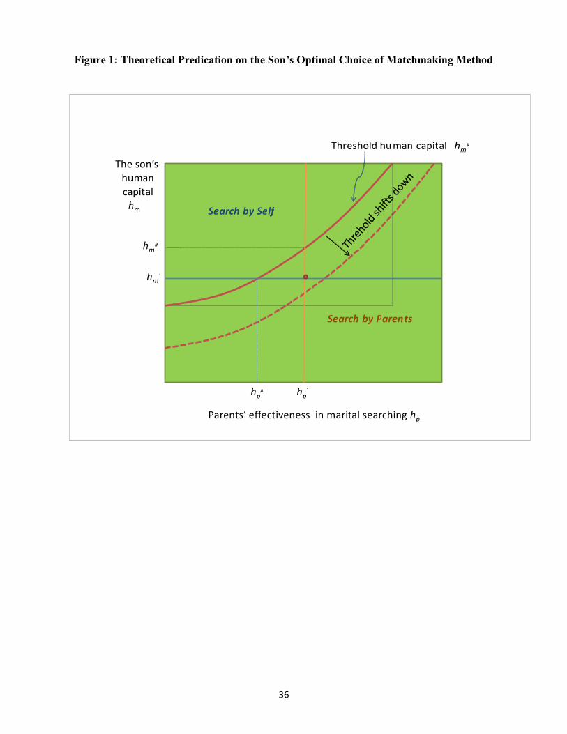
36

Figure 1: Theoretical Predication on the Son’s Optimal Choice of Matchmaking Method

P a r e n t s ’ e f f e c t i v e n e s s i n m a r i t a l s e a r c h i n g h p

T h e s o n ’ s

hu man

c apit al h m

Thr es hold hu man c apit al

h p #

h m #

h m ’

h p ’

h m #

Se arch b y Se lf

Se arch b y P aren ts

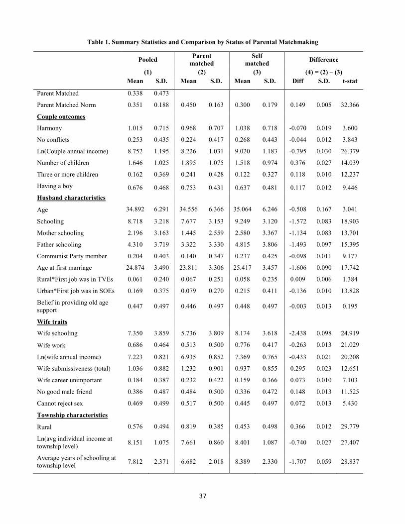
37

Table 1. Summary Statistics and Comparison by Status of Parental Matchmaking

Pooled

Parent

matched

Self

matched Difference

(1) (2) (3) (4) = (2) – (3)

Mean S.D. Mean S.D. Mean S.D. Diff S.D. t-stat

Parent Matched 0.338 0.473

Parent Matched Norm 0.351 0.188 0.450 0.163 0.300 0.179 0.149 0.005 32.366

Couple outcomes

Harmony 1.015 0.715 0.968 0.707 1.038 0.718 -0.070 0.019 3.600

No conflicts 0.253 0.435 0.224 0.417 0.268 0.443 -0.044 0.012 3.843

Ln(Couple annual income) 8.752 1.195 8.226 1.031 9.020 1.183 -0.795 0.030 26.379

Number of children 1.646 1.025 1.895 1.075 1.518 0.974 0.376 0.027 14.039

Three or more children 0.162 0.369 0.241 0.428 0.122 0.327 0.118 0.010 12.237

Having a boy 0.676 0.468 0.753 0.431 0.637 0.481 0.117 0.012 9.446

Husband characteristics

Age 34.892 6.291 34.556 6.366 35.064 6.246 -0.508 0.167 3.041

Schooling 8.718 3.218 7.677 3.153 9.249 3.120 -1.572 0.083 18.903

Mother schooling 2.196 3.163 1.445 2.559 2.580 3.367 -1.134 0.083 13.701

Father schooling 4.310 3.719 3.322 3.330 4.815 3.806 -1.493 0.097 15.395

Communist Party member 0.204 0.403 0.140 0.347 0.237 0.425 -0.098 0.011 9.177

Age at first marriage 24.874 3.490 23.811 3.306 25.417 3.457 -1.606 0.090 17.742

Rural*First job was in TVEs 0.061 0.240 0.067 0.251 0.058 0.235 0.009 0.006 1.384

Urban*First job was in SOEs 0.169 0.375 0.079 0.270 0.215 0.411 -0.136 0.010 13.828

Belief in providing old age

support 0.447 0.497 0.446 0.497 0.448 0.497 -0.003 0.013 0.195

Wife traits

Wife schooling 7.350 3.859 5.736 3.809 8.174 3.618 -2.438 0.098 24.919

Wife work 0.686 0.464 0.513 0.500 0.776 0.417 -0.263 0.013 21.029

Ln(wife annual income) 7.223 0.821 6.935 0.852 7.369 0.765 -0.433 0.021 20.208

Wife submissiveness (total) 1.036 0.882 1.232 0.901 0.937 0.855 0.295 0.023 12.651

Wife career unimportant 0.184 0.387 0.232 0.422 0.159 0.366 0.073 0.010 7.103

No good male friend 0.386 0.487 0.484 0.500 0.336 0.472 0.148 0.013 11.525

Cannot reject sex 0.469 0.499 0.517 0.500 0.445 0.497 0.072 0.013 5.430

Township characteristics

Rural 0.576 0.494 0.819 0.385 0.453 0.498 0.366 0.012 29.779

Ln(avg individual income at

township level) 8.151 1.075 7.661 0.860 8.401 1.087 -0.740 0.027 27.407

Average years of schooling at

township level 7.812 2.371 6.682 2.018 8.389 2.330 -1.707 0.059 28.837

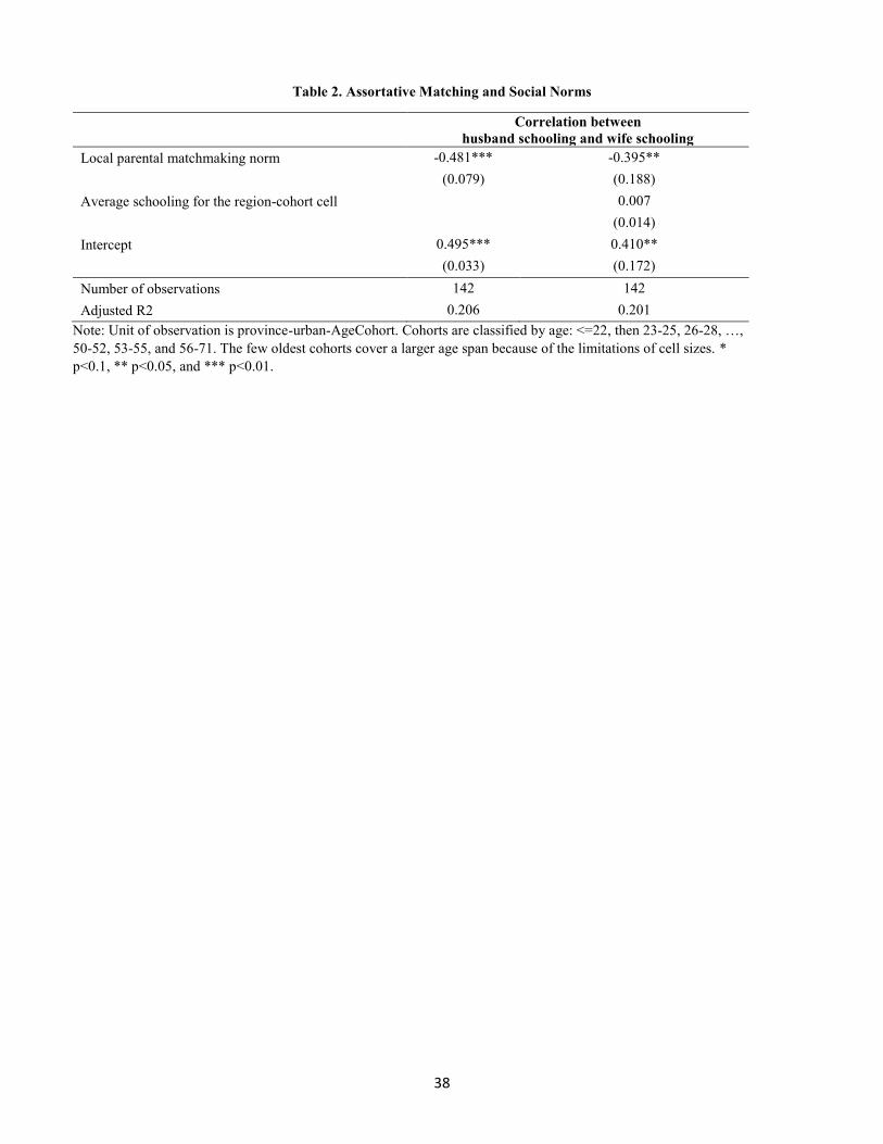
38

Table 2. Assortative Matching and Social Norms

Correlation between

husband schooling and wife schooling

Local parental matchmaking norm -0.481*** -0.395**

(0.079) (0.188)

Average schooling for the region-cohort cell 0.007

(0.014)

Intercept 0.495*** 0.410**

(0.033) (0.172)

Number of observations 142 142

Adjusted R2 0.206 0.201

Note: Unit of observation is province-urban-AgeCohort. Cohorts are classified by age: <=22, then 23-25, 26-28, …,

50-52, 53-55, and 56-71. The few oldest cohorts cover a larger age span because of the limitations of cell sizes. *

p<0.1, ** p<0.05, and *** p<0.01.

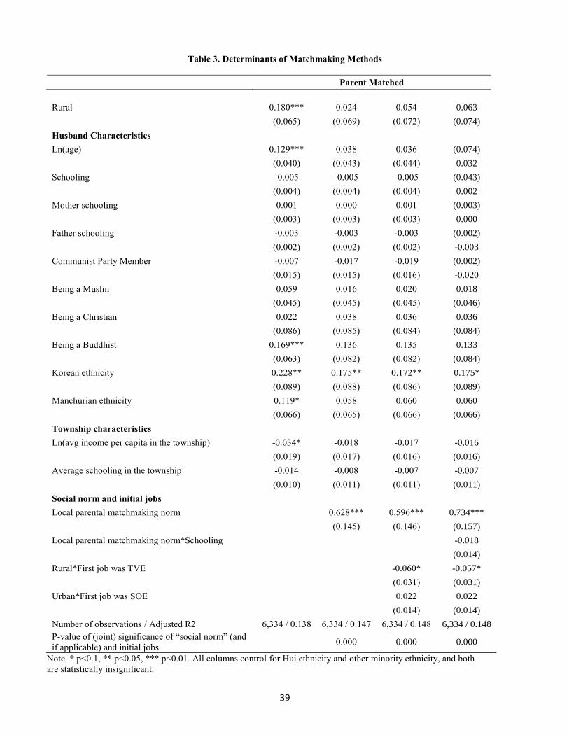
39

Table 3. Determinants of Matchmaking Methods

Parent Matched

Rural 0.180*** 0.024 0.054 0.063

(0.065) (0.069) (0.072) (0.074)

Husband Characteristics

Ln(age) 0.129*** 0.038 0.036 (0.074)

(0.040) (0.043) (0.044) 0.032

Schooling -0.005 -0.005 -0.005 (0.043)

(0.004) (0.004) (0.004) 0.002

Mother schooling 0.001 0.000 0.001 (0.003)

(0.003) (0.003) (0.003) 0.000

Father schooling -0.003 -0.003 -0.003 (0.002)

(0.002) (0.002) (0.002) -0.003

Communist Party Member -0.007 -0.017 -0.019 (0.002)

(0.015) (0.015) (0.016) -0.020

Being a Muslin 0.059 0.016 0.020 0.018

(0.045) (0.045) (0.045) (0.046)

Being a Christian 0.022 0.038 0.036 0.036

(0.086) (0.085) (0.084) (0.084)

Being a Buddhist 0.169*** 0.136 0.135 0.133

(0.063) (0.082) (0.082) (0.084)

Korean ethnicity 0.228** 0.175** 0.172** 0.175*

(0.089) (0.088) (0.086) (0.089)

Manchurian ethnicity 0.119* 0.058 0.060 0.060

(0.066) (0.065) (0.066) (0.066)

Township characteristics

Ln(avg income per capita in the township) -0.034* -0.018 -0.017 -0.016

(0.019) (0.017) (0.016) (0.016)

Average schooling in the township -0.014 -0.008 -0.007 -0.007

(0.010) (0.011) (0.011) (0.011)

Social norm and initial jobs

Local parental matchmaking norm 0.628*** 0.596*** 0.734***

(0.145) (0.146) (0.157)

Local parental matchmaking norm*Schooling -0.018

(0.014)

Rural*First job was TVE -0.060* -0.057*

(0.031) (0.031)

Urban*First job was SOE 0.022 0.022

(0.014) (0.014)

Number of observations / Adjusted R2 6,334 / 0.138 6,334 / 0.147 6,334 / 0.148 6,334 / 0.148

P-value of (joint) significance of “social norm” (and

if applicable) and initial jobs 0.000 0.000 0.000

Note. * p<0.1, ** p<0.05, *** p<0.01. All columns control for Hui ethnicity and other minority ethnicity, and both

are statistically insignificant.

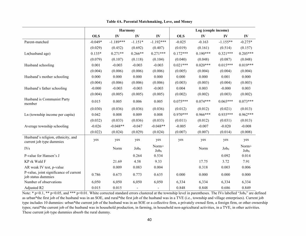
40

Table 4A. Parental Matchmaking, Love, and Money

Harmony Log (couple income)

OLS IV IV IV OLS IV IV IV

Parent-matched -0.049* -1.189*** -1.151* -1.192*** -0.025 -0.163 -1.155** -0.275*

(0.029) (0.452) (0.692) (0.407) (0.019) (0.161) (0.514) (0.157)

Ln(husband age) 0.135* 0.271** 0.266** 0.271*** 0.172*** 0.190*** 0.321*** 0.205***

(0.079) (0.107) (0.118) (0.104) (0.040) (0.048) (0.087) (0.048)

Husband schooling 0.001 -0.003 -0.003 -0.003 0.021*** 0.020*** 0.015*** 0.019***

(0.004) (0.006) (0.006) (0.006) (0.005) (0.004) (0.004) (0.004)

Husband’s mother schooling 0.000 0.000 0.000 0.000 0.000 0.000 0.001 0.000

(0.004) (0.006) (0.006) (0.006) (0.003) (0.003) (0.004) (0.003)

Husband’s father schooling -0.000 -0.003 -0.003 -0.003 0.004 0.003 -0.000 0.003

(0.004) (0.005) (0.005) (0.005) (0.002) (0.002) (0.003) (0.002)

Husband is Communist Party

member 0.015 0.005 0.006 0.005 0.075*** 0.074*** 0.065*** 0.073***

(0.030) (0.036) (0.036) (0.036) (0.012) (0.012) (0.021) (0.013)

Ln (township income per capita) 0.042 0.008 0.009 0.008 0.970*** 0.966*** 0.935*** 0.962***

(0.032) (0.033) (0.036) (0.033) (0.011) (0.012) (0.031) (0.013)

Average township schooling -0.026 -0.048** -0.047 -0.048** -0.005 -0.007 -0.020 -0.008

(0.022) (0.024) (0.029) (0.024) (0.007) (0.007) (0.014) (0.008)

Husband’s religion, ethnicity, and

current job type dummies yes yes yes yes yes yes yes yes

IVs Norm Job0 Norm+

Job0 Norm Job0

Norm+

Job0

P-value for Hansen’s J 0.264 0.534 0.092 0.014

KP rk Wald F 21.69 4.58 9.33 17.75 3.72 7.91

AR weak IV test, p-value 0.009 0.083 0.004 0.318 0.003 0.006

P-value, joint significance of current

job status dummies 0.786 0.673 0.773 0.635 0.000 0.000 0.000 0.000

Number of observations 6,050 6,050 6,050 6,050 6,334 6,334 6,334 6,334

Adjusted R2 0.015 0.015 - - 0.848 0.848 0.686 0.849

Note: * p<0.1, ** p<0.05, and *** p<0.01. White corrected standard errors clustered at the township level in parentheses. The IVs labelled “Job0” are defined

as urban*the first job of the husband was in an SOE, and rural*the first job of the husband was in a TVE (i.e., township and village enterprises). Current job

type includes 10 dummies: urban*the current job of the husband was in an SOE or a collective firm, a privately owned firm, a foreign firm, or other ownership

types; rural*the current job of the husband was in household production, in farming, in household non-agricultural activities, in a TVE, in other activities.

These current job type dummies absorb the rural dummy.

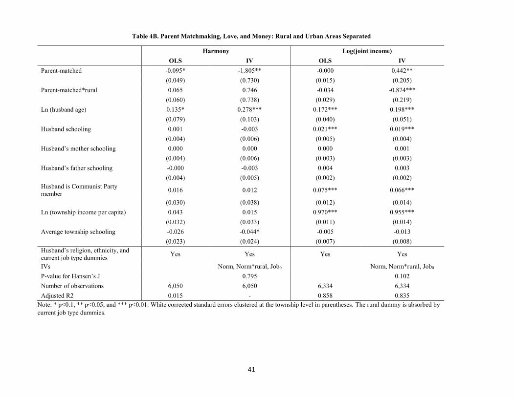
41

Table 4B. Parent Matchmaking, Love, and Money: Rural and Urban Areas Separated

Harmony Log(joint income)

OLS IV OLS IV

Parent-matched -0.095* -1.805** -0.000 0.442**

(0.049) (0.730) (0.015) (0.205)

Parent-matched*rural 0.065 0.746 -0.034 -0.874***

(0.060) (0.738) (0.029) (0.219)

Ln (husband age) 0.135* 0.278*** 0.172*** 0.198***

(0.079) (0.103) (0.040) (0.051)

Husband schooling 0.001 -0.003 0.021*** 0.019***

(0.004) (0.006) (0.005) (0.004)

Husband’s mother schooling 0.000 0.000 0.000 0.001

(0.004) (0.006) (0.003) (0.003)

Husband’s father schooling -0.000 -0.003 0.004 0.003

(0.004) (0.005) (0.002) (0.002)

Husband is Communist Party

member 0.016 0.012 0.075*** 0.066***

(0.030) (0.038) (0.012) (0.014)

Ln (township income per capita) 0.043 0.015 0.970*** 0.955***

(0.032) (0.033) (0.011) (0.014)

Average township schooling -0.026 -0.044* -0.005 -0.013

(0.023) (0.024) (0.007) (0.008)

Husband’s religion, ethnicity, and

current job type dummies Yes Yes Yes Yes

IVs Norm, Norm*rural, Job0 Norm, Norm*rural, Job0

P-value for Hansen’s J 0.795 0.102

Number of observations 6,050 6,050 6,334 6,334

Adjusted R2 0.015 - 0.858 0.835

Note: * p<0.1, ** p<0.05, and *** p<0.01. White corrected standard errors clustered at the township level in parentheses. The rural dummy is absorbed by

current job type dummies.

42

Table 5. Parent Matchmaking and Wife Schooling

Wife Schooling Wife Schooling

OLS IV OLS IV

Parent-matched -0.453*** -3.510** -0.055 -2.270**

(0.077) (1.408) (0.271) (1.084)

Parent-matched*Husband schooling -0.049* -0.138*

(0.029) (0.077)

Ln(husband age) -3.653*** -3.252*** -3.664*** -3.298***

(0.352) (0.341) (0.352) (0.328)

Husband schooling 0.250*** 0.234*** 0.268*** 0.286***

(0.022) (0.021) (0.020) (0.028)

Husband’s mother schooling 0.029* 0.031** 0.027* 0.026*

(0.015) (0.015) (0.015) (0.015)

Husband’s father schooling 0.028** 0.019 0.029** 0.021

(0.011) (0.014) (0.011) (0.013)

Husband is Communist Party member 0.261*** 0.233** 0.256** 0.220**

(0.100) (0.103) (0.100) (0.104)

Ln(township income per capita) 0.020 -0.075 0.022 -0.064

(0.086) (0.077) (0.087) (0.076)

Average township schooling 0.909*** 0.868*** 0.909*** 0.870***

(0.069) (0.068) (0.069) (0.069)

Husband’s religion, ethnicity, and current

job type dummies yes yes yes yes

IVs Norm+Job0 Norm+Job0

P-value for Hansen’s J 0.022 0.322

Number of observations 6,334 6,334 6,334 6,334

Adjusted R2 0.538 - 0.539 -

Note: * p<0.1, ** p<0.05, and *** p<0.01. White corrected standard errors clustered at the township level in parentheses. The rural dummy is absorbed

by current job type dummies.

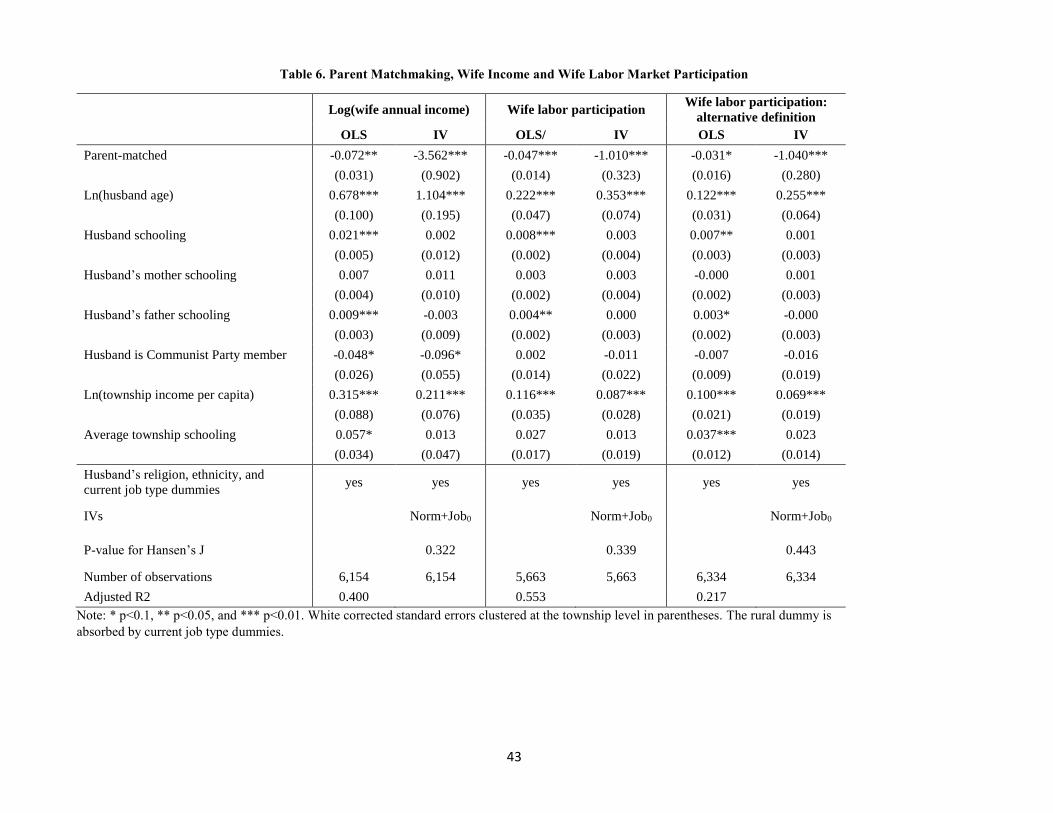
43

Table 6. Parent Matchmaking, Wife Income and Wife Labor Market Participation

Log(wife annual income) Wife labor participation Wife labor participation:

alternative definition

OLS IV OLS/ IV OLS IV

Parent-matched -0.072** -3.562*** -0.047*** -1.010*** -0.031* -1.040***

(0.031) (0.902) (0.014) (0.323) (0.016) (0.280)

Ln(husband age) 0.678*** 1.104*** 0.222*** 0.353*** 0.122*** 0.255***

(0.100) (0.195) (0.047) (0.074) (0.031) (0.064)

Husband schooling 0.021*** 0.002 0.008*** 0.003 0.007** 0.001

(0.005) (0.012) (0.002) (0.004) (0.003) (0.003)

Husband’s mother schooling 0.007 0.011 0.003 0.003 -0.000 0.001

(0.004) (0.010) (0.002) (0.004) (0.002) (0.003)

Husband’s father schooling 0.009*** -0.003 0.004** 0.000 0.003* -0.000

(0.003) (0.009) (0.002) (0.003) (0.002) (0.003)

Husband is Communist Party member -0.048* -0.096* 0.002 -0.011 -0.007 -0.016

(0.026) (0.055) (0.014) (0.022) (0.009) (0.019)

Ln(township income per capita) 0.315*** 0.211*** 0.116*** 0.087*** 0.100*** 0.069***

(0.088) (0.076) (0.035) (0.028) (0.021) (0.019)

Average township schooling 0.057* 0.013 0.027 0.013 0.037*** 0.023

(0.034) (0.047) (0.017) (0.019) (0.012) (0.014)

Husband’s religion, ethnicity, and

current job type dummies yes yes yes yes yes yes

IVs Norm+Job0 Norm+Job0 Norm+Job0

P-value for Hansen’s J 0.322 0.339 0.443

Number of observations 6,154 6,154 5,663 5,663 6,334 6,334

Adjusted R2 0.400 0.553 0.217

Note: * p<0.1, ** p<0.05, and *** p<0.01. White corrected standard errors clustered at the township level in parentheses. The rural dummy is

absorbed by current job type dummies.

44

Table 7. Parent Matchmaking and Wife Submissiveness

Wife Submissiveness

(overall)

Wife Career Not

Important No Good Male Friend Cannot Reject Sex

OLS IV OLS IV OLS IV OLS IV

Parent-matched 0.059* 1.982*** 0.007 0.610*** 0.050*** 1.026*** -0.000 0.358

(0.031) (0.674) (0.016) (0.212) (0.018) (0.367) (0.015) (0.275)

Ln(husband age) 0.084 -0.160 0.008 -0.071 0.008 -0.122 0.056 0.010

(0.092) (0.137) (0.032) (0.047) (0.056) (0.081) (0.048) (0.067)

Husband schooling -0.007 0.003 -0.002 0.001 -0.004 0.002 -0.002 0.001

(0.006) (0.014) (0.002) (0.004) (0.003) (0.006) (0.004) (0.005)

Husband’s mother schooling -0.006 -0.008 0.003* 0.003 -0.008*** -0.009** -0.002 -0.002

(0.004) (0.007) (0.002) (0.002) (0.003) (0.004) (0.003) (0.003)

Husband’s father schooling -0.009** -0.002 -0.005*** -0.003 -0.002 0.002 -0.003 -0.001

(0.004) (0.006) (0.002) (0.002) (0.002) (0.003) (0.002) (0.003)

Husband is Communist party member 0.031 0.049 0.012 0.018 0.050*** 0.059** -0.027* -0.023

(0.027) (0.044) (0.012) (0.016) (0.016) (0.024) (0.015) (0.016)

Ln (township income per capita) -0.132*** -0.079* -0.036*** -0.018 -0.042* -0.014 -0.049** -0.039*

(0.044) (0.045) (0.013) (0.016) (0.023) (0.024) (0.022) (0.021)

Average township schooling -0.094*** -0.072*** -0.025** -0.017 -0.022 -0.010 -0.042*** -0.038***

(0.028) (0.027) (0.010) (0.012) (0.015) (0.016) (0.015) (0.014)

Husband’s religion, ethnicity, and

current job type dummies

Yes Yes Yes Yes Yes Yes Yes Yes

IVs Norm+Job0 Norm+Job0 Norm+Job0 Norm+Job0

P-value for Hansen’s J 0.502 0.612 0.279 0.246

Number of observations 6,256 6,256 6,334 6,334 6,298 6,298 6,268 6,268

Adjusted R2 0.135 - 0.056 - 0.082 - 0.042 -

Note: * p<0.1, ** p<0.05, and *** p<0.01. White corrected standard errors clustered at the township level in parentheses. The rural dummy is absorbed by current

job type dummies.

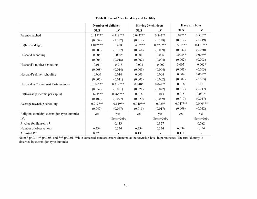
45

Table 8. Parent Matchmaking and Fertility

Number of children Having 3+ children Have any boys

OLS IV OLS IV OLS IV

Parent-matched 0.119*** 4.718*** 0.043*** 0.843** 0.027** 0.536**

(0.034) (1.257) (0.012) (0.338) (0.012) (0.219)

Ln(husband age) 1.042*** 0.438 0.432*** 0.327*** 0.536*** 0.470***

(0.209) (0.327) (0.064) (0.089) (0.042) (0.060)

Husband schooling 0.006 0.030* 0.001 0.006 0.005** 0.008**

(0.006) (0.018) (0.002) (0.004) (0.002) (0.003)

Husband’s mother schooling -0.011 -0.015 -0.002 -0.002 -0.005* -0.005*

(0.008) (0.014) (0.003) (0.004) (0.003) (0.003)

Husband’s father schooling -0.000 0.014 0.001 0.004 0.004 0.005**

(0.006) (0.011) (0.002) (0.002) (0.002) (0.003)

Husband is Communist Party member 0.176*** 0.219*** 0.040* 0.047** 0.016 0.021

(0.052) (0.081) (0.021) (0.022) (0.017) (0.017)

Ln(township income per capita) 0.623*** 0.765*** 0.018 0.043 0.015 0.031*

(0.107) (0.097) (0.029) (0.029) (0.017) (0.017)

Average township schooling -0.212*** -0.149** -0.040*** -0.029* -0.047*** -0.040***

(0.047) (0.067) (0.015) (0.017) (0.009) (0.012)

Religion, ethnicity, current job type dummies yes yes yes yes yes yes

IVs Norm+Job0 Norm+Job0 Norm+Job0

P-value for Hansen’s J 0.413 0.827 0.082

Number of observations 6,334 6,334 6,334 6,334 6,334 6,334

Adjusted R2 0.323 - 0.133 - 0.111 -

Note: * p<0.1, ** p<0.05, and *** p<0.01. White corrected standard errors clustered at the township level in parentheses. The rural dummy is

absorbed by current job type dummies.

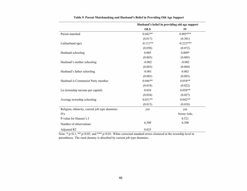
46

Table 9. Parent Matchmaking and Husband’s Belief in Providing Old Age Support

Husband’s belief in providing old age support

OLS IV

Parent-matched 0.042** 0.805***

(0.017) (0.301)

Ln(husband age) -0.121** -0.222***

(0.050) (0.072)

Husband schooling 0.005 0.009*

(0.003) (0.005)

Husband’s mother schooling -0.002 -0.002

(0.003) (0.004)

Husband’s father schooling -0.001 0.002

(0.003) (0.003)

Husband is Communist Party member 0.046** 0.054**

(0.018) (0.022)

Ln (township income per capital) 0.034 0.058**

(0.024) (0.027)

Average township schooling 0.031** 0.042**

(0.015) (0.018)

Religion, ethnicity, current job type dummies yes yes

IVs Norm+Job0

P-value for Hansen’s J 0.521

Number of observations 6,300 6,300

Adjusted R2 0.025 -

Note: * p<0.1, ** p<0.05, and *** p<0.01. White corrected standard errors clustered at the township level in

parentheses. The rural dummy is absorbed by current job type dummies.