Lossy joint source-channel coding in the ﬁnite blocklength...

1

Lossy joint source-channel coding

in the finite blocklength regimeVictoria Kostina, Student Member, IEEE, Sergio Verdu, Fellow, IEEE

Abstract—This paper finds new tight finite-blocklength boundsfor the best achievable lossy joint source-channel code rate,and demonstrates that joint source-channel code design bringsconsiderable performance advantage over a separate one in thenon-asymptotic regime. A joint source-channel code maps a blockof k source symbols onto a length−n channel codeword, and thefidelity of reproduction at the receiver end is measured by theprobability ǫ that the distortion exceeds a given threshold d. Formemoryless sources and channels, it is demonstrated that theparameters of the best joint source-channel code must satisfynC − kR(d) ≈

√

nV + kV(d)Q−1 (ǫ), where C and V are thechannel capacity and channel dispersion, respectively; R(d) andV(d) are the source rate-distortion and rate-dispersion functions;and Q is the standard Gaussian complementary cdf. Symbol-by-symbol (uncoded) transmission is known to achieve the Shannonlimit when the source and channel satisfy a certain probabilisticmatching condition. In this paper we show that even when thiscondition is not satisfied, symbol-by-symbol transmission is, insome cases, the best known strategy in the non-asymptotic regime.

Index Terms—Achievability, converse, finite blocklengthregime, joint source-channel coding, lossy source coding, memo-ryless sources, rate-distortion theory, Shannon theory.

I. INTRODUCTION

In the limit of infinite blocklengths, the optimal achievable

coding rates in channel coding and lossy data compression are

characterized by the channel capacity C and the source rate-

distortion function R(d), respectively [3]. For a large class

of sources and channels, in the limit of large blocklength,

the maximum achievable joint source-channel coding (JSCC)

rate compatible with vanishing excess distortion probability

is characterized by the ratio CR(d) [4]. A perennial question in

information theory is how relevant the asymptotic fundamental

limits are when the communication system is forced to operate

at a given fixed blocklength. The finite blocklength (delay)

constraint is inherent to all communication scenarios. In fact,

in many systems of current interest, such as real-time multi-

media communication, delays are strictly constrained, while

in packetized data communication, packets are frequently on

the order of 1000 bits. While computable formulas for the

This work was supported in part by the National Science Foundation (NSF)under Grant CCF-1016625 and by the Center for Science of Information(CSoI), an NSF Science and Technology Center, under Grant CCF-0939370.The work of V. Kostina was supported in part by the Natural Sciences andEngineering Research Council of Canada.

Portions of this paper were presented at the 2012 IEEE InternationalSymposium on Information Theory [1], and at the 2012 IEEE InformationTheory Workshop [2].

The authors are with the Department of Electrical Engineering,Princeton University, NJ 08544 USA (e-mail: [email protected];verdu@princeton. edu).

channel capacity and the source rate-distortion function are

available for a wide class of channels and sources, the luxury

of being able to compute exactly (in polynomial time) the non-

asymptotic fundamental limit of interest is rarely affordable.

Notable exceptions where the non-asymptotic fundamental

limit is indeed computable are almost lossless source coding

[5], [6], and JSCC over matched source-channel pairs [7]. In

general, however, one can at most hope to obtain bounds and

approximations to the information-theoretic non-asymptotic

fundamental limits.

Although non-asymptotic bounds can be distilled from

classical proofs of coding theorems, these bounds are rarely

satisfyingly tight in the non-asymptotic regime, as studied in

[8], [9] in the contexts of channel coding and lossy source

coding, respectively. For the JSCC problem, the classical

converse is based on the mutual information data process-

ing inequality, while the classical achievability scheme uses

separate source/channel coding (SSCC), in which the channel

coding block and the source coding block are optimized

separately without knowledge of each other. These conven-

tional approaches lead to disappointingly weak non-asymptotic

bounds. In particular, SSCC can be rather suboptimal non-

asymptotically. An accurate finite blocklength analysis there-

fore calls for novel upper and lower bounds that sandwich

tightly the non-asymptotic fundamental limit. Such bounds

were shown in [8] for the channel coding problem and in

[9] for the source coding problem. In this paper, we derive

new tight bounds for the JSCC problem, which hold in full

generality, without any assumptions on the source alphabet,

stationarity or memorylessness.

While numerical evaluation of the non-asymptotic upper and

lower bounds bears great practical interest (for example, to de-

cide how suboptimal with respect to the information-theoretic

limit a given blocklength-n code is), such bounds usually

involve cumbersome expressions that offer scant conceptual

insight. Somewhat ironically, to get an elegant, insightful

approximation of the non-asymptotic fundamental limit, one

must resort to an asymptotic analysis of these non-asymptotic

bounds. Such asymptotic analysis must be finer than that

based on the law of large numbers, which suffices to obtain

the asymptotic fundamental limit but fails to provide any

estimate of the speed of convergence to that limit. There

are two complementary approaches to a finer asymptotic

analysis: the large deviations analysis which leads to error

exponents, and the Gaussian approximation analysis which

leads to dispersion. The error exponent approximation and the

Gaussian approximation to the non-asymptotic fundamental

limit are tight in different operational regimes. In the former, a

2

rate which is strictly suboptimal with respect to the asymptotic

fundamental limit is fixed, and the error exponent measures

the exponential decay of the error probability to 0 as the

blocklength increases. The error exponent approximation is

tight if the error probability a system can tolerate is extremely

small. However, already for probability of error as low as 10−6

to 10−1, which is the operational regime for many high data

rate applications, the Gaussian approximation, which gives

the optimal rate achievable at a given error probability as

a function of blocklength, is tight [8], [9]. In the channel

coding problem, the Gaussian approximation of R⋆(n, ǫ),the maximum achievable finite blocklength coding rate at

blocklength n and error probability ǫ, is given by, for finite

alphabet stationary memoryless channels [8],

nR⋆(n, ǫ) = nC −√nV Q−1 (ǫ) +O (log n) (1)

where C and V are the channel capacity and dispersion,

respectively. In the lossy source coding problem, the Gaussian

approximation of R⋆(k, d, ǫ), the minimum achievable finite

blocklength coding rate at blocklength k and probability ǫ of

exceeding fidelity d, is given by, for stationary memoryless

sources [9],

kR⋆(k, d, ǫ) = kR(d) +√kV(d)Q−1 (ǫ) +O (log k) (2)

where R(d) and V(d) are the rate-distortion and the rate-

dispersion functions, respectively.

For a given code, the excess distortion constraint, which is

the figure of merit in this paper as well as in [9], is, in a

way, more fundamental than the average distortion constraint,

because varying d over its entire range and evaluating the

probability of exceeding d gives full information about the

distribution (and not just its mean) of the distortion incurred at

the decoder output. Following the philosophy of [8], [9], in this

paper we perform the Gaussian approximation analysis of our

new bounds to show that k, the maximum number of source

symbols transmissible using a given channel blocklength n,

must satisfy

nC − kR(d) =√nV + kV(d)Q−1 (ǫ) +O (logn) (3)

under the fidelity constraint of exceeding a given distortion

level d with probability ǫ. In contrast, if, following the SSCC

paradigm, we just concatenate the channel code in (1) and the

source code in (2), we obtain

nC − kR(d) ≤ minη+ζ≤ǫ

{√nV Q−1 (η) +

√kV(d)Q−1 (ζ)

}

+O (logn) (4)

which is usually strictly suboptimal with respect to (3).

In addition to deriving new general achievability and con-

verse bounds for JSCC and performing their Gaussian ap-

proximation analysis, in this paper we revisit the dilemma of

whether one should or should not code when operating under

delay constraints. Gastpar et al. [7] gave a set of necessary and

sufficient conditions on the source, its distortion measure, the

channel and its cost function in order for symbol-by-symbol

transmission to attain the minimum average distortion. In these

curious cases, the source and the channel are probabilistically

matched. In the absence of channel cost constraints, we show

that whenever the source and the channel are probabilistically

matched so that symbol-by-symbol coding achieves the min-

imum average distortion, it also achieves the dispersion of

joint source-channel coding. Moreover, even in the absence of

such a match between the source and the channel, symbol-

by-symbol transmission, though asymptotically suboptimal,

might outperform in the non-asymptotic regime not only

separate source-channel coding but also our random-coding

achievability bound.

Prior research relating to finite blocklength analysis of JSCC

includes the work of Csiszar [10], [11] who demonstrated

that the error exponent of joint source-channel coding out-

performs that of separate source-channel coding. For discrete

source-channel pairs with average distortion criterion, Pilc’s

achievability bound [12], [13] applies. For the transmission

of a Gaussian source over a discrete channel under the

average mean square error constraint, Wyner’s achievability

bound [14], [15] applies. Non-asymptotic achievability and

converse bounds for a graph-theoretic model of JSCC have

been obtained by Csiszar [16]. Most recently, Tauste Campo et

al. [17] showed a number of finite-blocklength random-coding

bounds applicable to the almost-lossless JSCC setup, while

Wang et al. [18] found the dispersion of JSCC for sources

and channels with finite alphabets.

The rest of the paper is organized as follows. Section II

summarizes basic definitions and notation. Sections III and

IV introduce the new converse and achievability bounds to

the maximum achievable coding rate, respectively. A Gaussian

approximation analysis of the new bounds is presented in

Section V. The evaluation of the bounds and the approximation

is performed for two important special cases: the transmission

of a binary memoryless source (BMS) over a binary symmetric

channel (BSC) with bit error rate distortion (Section VI) and

the transmission of a Gaussian memoryless source (GMS) with

mean-square error distortion over an AWGN channel with a

total power constraint (Section VII). Section VIII focuses on

symbol-by-symbol transmission.

II. DEFINITIONS

A lossy source-channel code is a pair of (possibly random-

ized) mappings f : M 7→ X and g : Y 7→ M. A distortion

measure d : M×M 7→ [0,+∞] is used to quantify the per-

formance of the lossy code. A cost function c : X 7→ [0,+∞]may be imposed on the channel inputs. The channel is used

without feedback.

Definition 1. The pair (f, g) is a (d, ǫ, α) lossy source-

channel code for {M, X , Y, M, PS , d, PY |X , c} if

P [d (S, g(Y )) > d] ≤ ǫ and either E [c(X)] ≤ α (average

cost constraint) or c(X) ≤ α a.s. (maximal cost constraint),

where f(S) = X (see Fig. 1). In the absence of an input cost

constraint we simplify the terminology and refer to the code

as (d, ǫ) lossy source-channel code.

The special case d = 0 and d(s, z) = 1 {s 6= z} corresponds

to almost-lossless compression. If, in addition, PS is equiprob-

able on an alphabet of cardinality |M| = |M| =M , a (0, ǫ, α)code in Definition 1 corresponds to an (M, ǫ, α) channel code

3

PY |X

|

X Y ZS

P [d (S,Z) > d] ≤ ǫ

f = g

Fig. 1. A (d, ǫ) joint source-channel code.

(i.e. a code with M codewords and average error probability ǫand cost α). On the other hand, if PY |X is an identity mapping

on an alphabet of cardinality M without cost constraints, a

(d, ǫ) code in Definition 1 corresponds to an (M,d, ǫ) lossy

compression code (as e.g. defined in [9]).

As our bounds in Sections III and IV do not foist a Cartesian

structure on the underlying alphabets, we state them in the one-

shot paradigm of Definition 1. When we apply those bounds

to the block coding setting, transmitted objects indeed become

vectors, and Definition 2 below comes into play.

Definition 2. In the conventional fixed-to-fixed (or block)

setting in which X and Y are the n−fold Cartesian prod-

ucts of alphabets A and B, M and M are the k−fold

Cartesian products of alphabets S and S, and dk : Sk ×Sk 7→ [0,+∞], cn : An 7→ [0,+∞], a (d, ǫ, α) code for

{Sk, An, Bn, Sk, PSk , dk, PY n|Xn , cn} is called a

(k, n, d, ǫ, α) code (or a (k, n, d, ǫ) code if there is no cost

constraint).

Definition 3. Fix ǫ, d, α and the channel blocklength n.

The maximum achievable source blocklength and coding rate

(source symbols per channel use) are defined by, respectively

k⋆(n, d, ǫ, α) = sup {k : ∃(k, n, d, ǫ, α) code} (5)

R(n, d, ǫ, α) =1

nk⋆(n, d, ǫ, α) (6)

Alternatively, fix ǫ, α, source blocklength k and channel

blocklength n. The minimum achievable excess distortion is

defined by

D(k, n, ǫ, α) = inf {d : ∃(k, n, d, ǫ, α) code} (7)

Denote, for a given PY |X and a cost function c : X 7→[0,+∞],

C(α) = supPX :

E[c(X)]≤α

I(X ;Y ) (8)

and, for a given PS and a distortion measure d : M×M 7→[0,+∞],

RS(d) = infPZ|S :

E[d(S,Z)]≤d

I(S;Z) (9)

We impose the following basic restrictions on PY |X , PS , the

input-cost function and the distortion measure:

(a) RS(d) is finite for some d, i.e. dmin <∞, where

dmin = inf {d : RS(d) <∞} ; (10)

(b) The infimum in (9) is achieved by a unique PZ⋆|S ;

(c) The supremum in (8) is achieved by a unique PX⋆ .

The dispersion, which serves to quantify the penalty on the

rate of the best JSCC code induced by the finite blocklength,

is defined as follows.

Definition 4. Fix α and d ≥ dmin. The rate-dispersion func-

tion of joint source-channel coding (source samples squared

per channel use) is defined as

V(d, α) = limǫ→0

lim supn→∞

n(C(α)R(d) −R(n, d, ǫ, α)

)2

2 loge1ǫ

(11)

where C(α) and R(d) are the channel capacity-cost and

source rate-distortion functions, respectively.1

The distortion-dispersion function of joint source-channel

coding is defined as

W(R,α) = limǫ→0

lim supn→∞

n(D(C(α)R

)−D(nR, n, ǫ, α)

)2

2 loge1ǫ

(12)

where D(·) is the distortion-rate function of the source.

If there is no cost constraint, we will simplify notation by

dropping α from (5), (6), (7), (8), (11) and (12).

Definition 5 (d−tilted information [9]). For d > dmin, the

d−tilted information in s is defined as2

S(s, d) = log1

E [exp (λ⋆d− λ⋆d(s, Z⋆))](13)

where the expectation is with respect to PZ⋆ , i.e. the uncon-

ditional distribution of the reproduction random variable that

achieves the infimum in (9), and

λ⋆ = −R′S(d) (14)

The following properties of d−tilted information, proven in

[19], are used in the sequel.

S(s, d) = ıS;Z⋆(s; z) + λ⋆d(s, z)− λ⋆d (15)

E [S(s, d)] = RS(d) (16)

E [exp (λ⋆d− λ⋆d(S, z) + S(S, d))] ≤ 1 (17)

where (15) holds for P ⋆Z-almost every z, while (17) holds for

all z ∈ M, and

ıS;Z(s; z) = logdPZ|S=sdPZ

(z) (18)

denotes the information density of the joint distribution PSZat (s, z). We can define the right side of (18) for a given

(PZ|S , PZ) even if there is no PS such that the marginal of

PSPZ|S is PZ . We use the same notation ıS;Z for that more

general function. To extend Definition 5 to the lossless case,

for discrete random variables we define 0-tilted information as

S(s, 0) = ıS(s) (19)

1While for memoryless sources and channels, C(α) = C(α) and R(d) =RS(d) given by (8) and (9) evaluated with single-letter distributions, it isimportant to distinguish between the operational definitions and the extremalmutual information quantities, since the core results in this paper allow formemory.

2All log’s and exp’s are in an arbitrary common base.

4

where

ıS(s) = log1

PS(s)(20)

is the information in outcome s ∈ M.

The distortion d-ball centered at s ∈ M is denoted by

Bd(s) = {z ∈ M : d(s, z) ≤ d}. (21)

Given (PX , PY |X), we write PX → PY |X → PY to

indicate that PY is the marginal of PXPY |X , i.e. PY (y) =∑x∈X PY |X(y|x)PX(x). 3

So as not to clutter notation, in Sections III and IV we

assume that there are no cost constraints. However, all results

in those sections generalize to the case of a maximal cost

constraint by considering X whose distribution is supported

on the subset of allowable channel inputs:

F(α) = {x ∈ X : c(x) ≤ α} (22)

rather than the entire channel input alphabet X .

III. CONVERSES

A. Converses via d-tilted information

Our first result is a general converse bound.

Theorem 1 (Converse). The existence of a (d, ǫ) code for Sand PY |X requires that

ǫ ≥ infPX|S

supγ>0

{supPY

P[S(S, d)− ıX;Y (X ;Y ) ≥ γ

]

− exp (−γ)}

(23)

≥ supγ>0

{supPY

E

[infx∈X

P[S(S, d)− ıX;Y (x;Y ) ≥ γ | S

]]

− exp (−γ)}

(24)

where in (23), S − X − Y , and the conditional probability

in (24) is with respect to Y distributed according to PY |X=x

(independent of S), and

ıX;Y (x; y) = logdPY |X=x

dPY(y) (25)

Proof. Fix γ and the (d, ǫ) code (PX|S , PZ|Y ). Fix an arbitrary

probability measure PY on Y . Let PY → PZ|Y → PZ . We

3We write summations over alphabets for simplicity. Unless stated other-wise, all our results hold for abstract probability spaces.

can write the probability in the right side of (23) as

P[S(S, d)− ıX;Y (X ;Y ) ≥ γ

]

= P[S(S, d)− ıX;Y (X ;Y ) ≥ γ, d(S;Z) > d

]

+ P[S(S, d)− ıX;Y (X ;Y ) ≥ γ, d(S;Z) ≤ d

](26)

≤ ǫ

+∑

s∈MPS(s)

∑

x∈XPX|S(x|s)

∑

y∈Y

∑

z∈Bd(s)

PZ|Y (z|y)

· PY |X(y|x)1{PY |X(y|x) ≤ PY (y) exp (S(s, d)− γ)

}

(27)

≤ ǫ + exp (−γ)∑

s∈MPS(s) exp (S(s, d))

∑

y∈YPY (y)

·∑

z∈Bd(s)

PZ|Y (z|y)∑

x∈XPX|S(x|s) (28)

= ǫ + exp (−γ)∑


∑

y∈YPY (y)

·∑

z∈Bd(s)

PZ|Y (z|y) (29)

= ǫ + exp (−γ)∑

s∈MPS(s) exp (S(s, d))PZ(Bd(s)) (30)

≤ ǫ + exp (−γ)∑

z∈M

PZ(z)∑

s∈MPS(s)

· exp (S(s, d) + λ⋆d− λ⋆d(s, z)) (31)

≤ ǫ + exp (−γ) (32)

where (32) is due to (17). Optimizing over γ > 0 and PY ,

we get the best possible bound for a given encoder PX|S . To

obtain a code-independent converse, we simply choose PX|Sthat gives the weakest bound, and (23) follows. To show (24),

we weaken (23) as

ǫ ≥ supγ>0

{supPY

infPX|S

P[S(S, d)− ıX;Y (X ;Y ) ≥ γ

]

− exp (−γ)}

(33)

and observe that for any PY ,

infPX|S

P[S(S, d)− ıX;Y (X ;Y ) ≥ γ

]

=∑

s∈MPS(s) inf

PX|S=s

∑

x∈XPX|S(x|s)

·∑

y∈YPY |X(y|x)1

{S(s, d)− ıX;Y (x; y) ≥ γ

}(34)

=∑

s∈MPS(s)

· infx∈X

∑

y∈YPY |X(y|x)1

{S(s, d)− ıX;Y (x; y) ≥ γ

}(35)

= E

[infx∈X

P[S(S, d)− ıX;Y (x;Y ) ≥ γ | S

]](36)

5

An immediate corollary to Theorem 1 is the following

result.

Theorem 2 (Converse). Assume that there exists a distribution

PY such that the distribution of ıX;Y (x;Y ) (according to

PY |X=x) does not depend on the choice of x ∈ X . If a (d, ǫ)code for S and PY |X exists, then

ǫ ≥ supγ>0

{P[S(S, d)− ıX;Y (x;Y ) ≥ γ

]− exp (−γ)

}

(37)

for an arbitrary x ∈ X . The probability measure P in (37) is

generated by PSPY |X=x.

Proof. Under the assumption, the conditional probability in

the right side of (24) is the same regardless of the choice of

x ∈ X .

The next result generalizes Theorem 1. When we apply

Theorem 3 in Section V to find the dispersion of JSCC, we

will let T be the number of channel input types, and we will let

W be the type of the channel input block. If T = 1, Theorem

3 reduces to Theorem 1.

Theorem 3 (Converse). The existence of a (d, ǫ) code for Sand PY |X requires that

ǫ ≥ infPX|S

maxγ>0,T

{− T exp (−γ)

+ supY ,W :

S−(X,W )−Y

P[S(S, d)− ıX;Y |W (X ;Y |W ) ≥ γ

]}

(38)

≥ maxγ>0,T

{− T exp (−γ)

+ supY ,W

E

[infx∈X

P[S(S, d)− ıX;Y |W (x;Y |W ) ≥ γ | S

]]}

(39)

where T is a positive integer, the random variable W takes

values on {1, . . . , T }, and

ıX;Y |W (x; y|t) = logPY |X=x,W=t

PY |W=t

(y) (40)

and in (39), the probability measure is generated by

PSPW |X=xPY |X=x,W .

Proof. Fix a possibly randomized (d, ǫ) code {PX|S, PZ|Y },

a positive scalar γ, a positive integer T , an auxiliary ran-

dom variable W that satisfies S − (X,W ) − Y , and a

conditional probability distribution PY |W : {1, . . . T } 7→ Y .

Let PY |W=t → PZ|Y → PZ|W=t, i.e. PZ|W=t(z) =

∑y∈Y PZ|Y (z|y)PY |W=t(y), for all t. Write

P[S(S, d)− ıX;Y |W (X ;Y |W ) ≥ γ

]

≤ ǫ +∑

s∈MPS(s)

T∑

t=1

PW |S(t|s)∑

x∈XPX|S,W (x|s, t)

·∑

y∈YPY |X,W (y|x, t)

∑

z∈Bd(s)

PZ|Y (z|y)

· 1{PY |X,W (y|x, t) ≤ PY |W=t(y) exp (S(s, d) − γ)

}

(41)

≤ ǫ + exp (−γ)∑


T∑

t=1

PW |S(t|s)

·∑

y∈YPY |W (y|t)

∑

z∈Bd(s)

PZ|Y (z|y)∑

x∈XPX|S,W (x|s, t)

(42)

≤ ǫ + exp (−γ)T∑

t=1

∑


∑

y∈YPY |W (y|t)

·∑

z∈Bd(s)

PZ|Y (z|y) (43)

≤ ǫ + exp (−γ)T∑

t=1

∑

s∈MPS(s) exp (S(s, d))PZ|W=t(Bd(s))

(44)

≤ ǫ + exp (−γ)T∑

t=1

∑

s∈MPS(s)

∑

z∈M

PZ|W=t(z)

· exp (S(s, d) + λ⋆d− λ⋆d(s, z)) (45)

≤ ǫ + T exp (−γ) (46)

where (46) is due to (17). Optimizing over γ, T and the

distributions of the auxiliary random variables Y and W , we

obtain the best possible bound for a given encoder PX|S .

To obtain a code-independent converse, we simply choose

PX|S that gives the weakest bound, and (38) follows. To show

(39), we weaken (38) by restricting the sup to W satisfying

S−X−W and changing the order of inf and sup as follows:

maxγ>0,T

supY ,W :

S−(X,W )−YS−X−W

infPX|S

(47)

Observe that for any legitimate choice of Y and W ,

infPX|S

P[S(S, d)− ıX;Y |W (X ;Y |W ) ≥ γ

](48)

=∑

s∈MPS(s) inf

PX|S=s

∑

x∈XPX|S(x|s)

T∑

t=1

PW |X(t|x)

·∑

y∈YPY |X,W (y|x, t)1

{S(s, d)− ıX;Y |W (x; y|t) ≥ γ

}

(49)

=∑

s∈MPS(s) inf

x∈X

T∑

t=1

PW |X(t|x)∑

y∈YPY |X,W (y|x, t)

· 1{S(s, d)− ıX;Y |W (x; y|t) ≥ γ

}(50)

which is equal to the expectation on the right side of (39).

6

Remark 1. Theorems 1, 2 and 3 still hold in the case d = 0 and

d(x, y) = 1 {x 6= y}, which corresponds to almost-lossless

data compression. Indeed, recalling (19), it is easy to see that

the proof of Theorem 1 applies, skipping the now unnecessary

step (31), and, therefore, (23) reduces to

ǫ ≥ infPX|S

supγ>0

{supPY

P[ıS(S)− ıX;Y (X ;Y ) ≥ γ

]

− exp (−γ)}

(51)

Similar modification can be applied to the proof of Theorem

3.

Remark 2. Our converse for lossy source coding in [9,

Theorem 7] can be viewed as a particular case of the result

in Theorem 2. Indeed, if X = Y = {1, . . . ,M} and

PY |X(m|m) = 1, PY (1) = . . . = PY (M) = 1M , then (37)

becomes

ǫ ≥ supγ>0

P [S(S, d) ≥ logM + γ]− exp (−γ) (52)

which is precisely [9, Theorem 7].

B. Converses via hypothesis testing and list decoding

To show a joint source-channel converse in [11], Csiszar

used a list decoder, which outputs a list of L elements

drawn from M. While traditionally list decoding has only

been considered in the context of finite alphabet sources, we

generalize the setting to sources with abstract alphabets. In our

setup, the encoder is the random transformation PX|S , and the

decoder is defined as follows.

Definition 6 (List decoder). Let L be a positive real number,

and let QS be a measure on M. An (L,QS) list decoder

is a random transformation PS|Y , where S takes values on

QS-measurable sets with QS-measure not exceeding L:

QS

(S)≤ L (53)

Even though we keep the standard “list” terminology, the

decoder output need not be a finite or countably infinite set.

The error probability with this type of list decoding is the

probability that the source outcome S does not belong to the

decoder output list for Y :

1−∑

x∈X

∑

y∈Y

∑

s∈M(L)

∑

s∈sPS|Y (s|y)PY |X(y|x)PX|S(x|s)PS(s)

(54)

where M(L) is the set of all QS-measurable subsets of Mwith QS-measure not exceeding L.

Definition 7 (List code). An (ǫ, L,QS) list code is a pair

of random transformations (PX|S , PS|Y ) such that (53) holds

and the list error probability (54) does not exceed ǫ.

Of course, letting QS = US , where US is the counting

measure on M, we recover the conventional list decoder

definition where the smallest scalar that satisfies (53) is an

integer. The almost-lossless JSCC setting (d = 0) in Definition

1 corresponds to L = 1, QS = US . If the source is analog

(has a continuous distribution), it is reasonable to let QS be

the Lebesgue measure.

Any converse for list decoding implies a converse for

conventional decoding. To see why, observe that any (d, ǫ)lossy code can be converted to a list code with list error

probability not exceeding ǫ by feeding the lossy decoder output

to a function that outputs the set of all source outcomes swithin distortion d from the output z ∈ M of the original

lossy decoder. In this sense, the set of all (d, ǫ) lossy codes is

included in the set of all list codes with list error probability

≤ ǫ and list size

L = maxz∈M

QS ({s : d(s, z) ≤ d}) (55)

Denote by

βα(P,Q) = minPW |X :

P[W=1]≥α

Q [W = 1] (56)

the optimal performance achievable among all randomized

tests PW |X : X → {0, 1} between probability distributions Pand Q on X (1 indicates that the test chooses P ).4 In fact, Qneed not be a probability measure, it just needs to be σ-finite

in order for the Neyman-Pearson lemma and related results to

hold.

The hypothesis testing converse for channel coding [8,

Theorem 27] can be generalized to joint source-channel coding

with list decoding as follows.

Theorem 4 (Converse). Fix PS and PY |X , and let QS be

a σ-finite measure. The existence of an (ǫ, L,QS) list code

requires that

infPX|S

supPY

β1−ǫ(PSPX|SPY |X , QSPX|SPY ) ≤ L (57)

where the supremum is over all probability measures PYdefined on the channel output alphabet Y .

Proof. Fix QS , the encoder PX|S , and an auxiliary σ-finite

conditional measure QY |XS . Consider the (not necessarily

optimal) test for deciding between PSXY = PSPX|SPY |X and

QSXY = QSPX|SQY |XS which chooses PSXY if S belongs

to the decoder output list. Note that this is a hypothetical test,

which has access to both the source outcome and the decoder

output.

According to P, the probability measure generated by

PSXY , the probability that the test chooses PSXY is given

by

P

[S ∈ S

]≥ 1− ǫ (58)

Since Q

[S ∈ S

]is the measure of the event that the test

chooses PSXY when QSXY is true, and the optimal test

cannot perform worse than the possibly suboptimal one that

we selected, it follows that

β1−ǫ(PSPX|SPY |X , QSPX|SQY |XS) ≤ Q

[S ∈ S

](59)

4Throughout, P , Q denote distributions, whereas P, Q are used for thecorresponding probabilities of events on the underlying probability space.

7

Now, fix an arbitrary probability measure PY on Y . Choosing

QY |XS = PY , the inequality in (59) can be weakened as

follows.

Q

[S ∈ S

]

=∑

y∈YPY (y)

∑

s∈M(L)

PS|Y (s|y)∑

s∈sQS(s)

∑

x∈XPX|S(x|s)

(60)

=∑

y∈YPY (y)

∑

s∈M(L)

PS|Y (s|y)∑

s∈sQS(s) (61)

≤∑

y∈YPY (y)

∑

s∈M(L)

PS|Y (s|y)L (62)

= L (63)

Optimizing the bound over PY and choosing PX|S that yields

the weakest bound in order to obtain a code-independent

converse, (57) follows.

Remark 3. Similar to how Wolfowitz’s converse for channel

coding can be obtained from the meta-converse for channel

coding [8], the converse for almost-lossless joint source-

channel coding in (51) can be obtained by appropriately

weakening (57) with L = 1. Indeed, invoking [8]

βα(P,Q) ≥ 1

γ

(α− P

[dP

dQ> γ

])(64)

and letting QS = US in (57), where US is the counting

measure on M, we have

1 ≥ infPX|S

supPY

β1−ǫ(PSPX|SPY |X , USPX|SPY ) (65)

≥ infPX|S

supPY

supγ>0

1

γ

(1− ǫ− P

[ıX;Y (X ;Y )−ıS(S)> log γ

])

(66)

which upon rearranging yields (51).

In general, computing the infimum in (57) is challenging.

However, if the channel is symmetric (in a sense formalized

in the next result), β1−ǫ(PSPX|SPY |X , USPX|SPY ) is inde-

pendent of PX|S .

Theorem 5 (Converse). Fix a probability measure PY . Assume

that the distribution of ıX;Y (x;Y ) does not depend on x ∈X under either PY |X=x or PY . Then, the existence of an

(ǫ, L,QS) list code requires that

β1−ǫ(PSPY |X=x, QSPY ) ≤ L (67)

where x ∈ X is arbitrary.

Proof. The Neyman-Pearson lemma (e.g. [20]) implies that the

outcome of the optimum binary hypothesis test between P and

Q only depends on the observation through dPdQ . In particular,

the optimum binary hypothesis test W ⋆ for deciding between

PSPX|SPY |X and QSPX|SPY satisfies

W ⋆ − (S, ıX;Y (X ;Y ))− (S,X, Y ) (68)

For all s ∈ M, x ∈ X , we have

P [W ⋆ = 1|S = s,X = x]

= E [P [W ⋆ = 1|X = x, S = s, Y ]] (69)

= E[P[W ⋆ = 1|S = s, ıX;Y (X ;Y ) = ıX;Y (x;Y )

]](70)

=∑

y∈YPY |X(y|x)PW⋆|S, ıX;Y (X;Y )(1|s, ıX;Y (x; y)) (71)

= P [W ⋆ = 1|S = s] (72)

and

Q [W ⋆ = 1|S = s,X = x] = Q [W ⋆ = 1|S = s] (73)

where

• (70) is due to (68),

• (71) uses the Markov property S −X − Y ,

• (72) follows from the symmetry assumption on the dis-

tribution of ıX;Y (x, Y ),• (73) is obtained similarly to (71).

Since (72), (73) imply that the optimal test achieves the same

performance (that is, the same P [W ⋆ = 1] and Q [W ⋆ = 1])regardless of PX|S , we choose PX|S = 1X(x) for some x ∈ Xin the left side of (57) to obtain (67).

Remark 4. In the case of finite channel input and output

alphabets, the channel symmetry assumption of Theorem 5

holds, in particular, if the rows of the channel transition

probability matrix are permutations of each other, and PY n is

the equiprobable distribution on the (n-dimensional) channel

output alphabet, which, coincidentally, is also the capacity-

achieving output distribution. For Gaussian channels with

equal power constraint, which corresponds to requiring the

channel inputs to lie on the power sphere, any spherically-

symmetric PY n satisfies the assumption of Theorem 5.

IV. ACHIEVABILITY

Given a source code (f(M)s , g

(M)s ) of size M , and a channel

code (f(M)c , g

(M)c ) of size M , we may concatenate them to

obtain the following sub-class of the source-channel codes

introduced in Definition 1:

Definition 8. An (M,d, ǫ) source-channel code is a (d, ǫ)source-channel code such that the encoder and decoder map-

pings satisfy

f = f(M)c ◦ f(M)

s (74)

g = g(M)c ◦ g(M)

s (75)

where

f(M)s : M 7→ {1, . . . ,M} (76)

f(M)c : {1, . . . ,M} 7→ X (77)

g(M)c : Y 7→ {1, . . . ,M} (78)

g(M)s : {1, . . . ,M} 7→ M (79)

(see Fig. 2).

Note that an (M,d, ǫ) code is an (M + 1, d, ǫ) code.

The conventional separate source-channel coding paradigm

corresponds to the special case of Definition 8 in which the

8

PY |X

|

X Y ZS

P [d (S,Z) > d] ≤ ǫ

∈ {1, . . . ,M}n

∈ {1, . . . ,M}nf

(M)s f

(M)c g

(M)c

g(M)s

Fig. 2. An (M, d, ǫ) joint source-channel code.

source code (f(M)s , g

(M)s ) is chosen without knowledge of

PY |X and the channel code (f(M)c , g

(M)c ) is chosen without

knowledge of PS and the distortion measure d. A pair of

source and channel codes is separation-optimal if the source

code is chosen so as to minimize the distortion (average

or excess) when there is no channel, whereas the channel

code is chosen so as to minimize the worst-case (over source

distributions) average error probability:

maxPU

P

[U 6= g(M)

c (Y )]

(80)

where X = f(M)c (U) and U takes values on {1, . . . ,M}. If

both the source and the channel code are chosen separation-

optimally for their given sizes, the separation principle guar-

antees that under certain quite general conditions (which

encompass the memoryless setting, see [21]) the asymptotic

fundamental limit of joint source-channel coding is achiev-

able. In the finite blocklength regime, however, such SSCC

construction is, in general, only suboptimal. Within the SSCC

paradigm, we can obtain an achievability result by further

optimizing with respect to the choice of M :

Theorem 6 (Achievability, SSCC). Fix PY |X , d and PS .

Denote by ǫ⋆(M) the minimum achievable worst-case average

error probability among all transmission codes of size M , and

the minimum achievable probability of exceeding distortion dwith a source code of size M by ǫ⋆(M,d).

Then, there exists a (d, ǫ) source-channel code with

ǫ ≤ minM

{ǫ⋆(M) + ǫ⋆(M,d)} (81)

Bounds on ǫ⋆(M) and ǫ⋆(M,d) have been obtained recently

in [8] and [9], respectively.5

Definition 8 does not rule out choosing the source code

based on the knowledge of PY |X or the channel code based

on the knowledge of PS , d and d. One of the interesting

conclusions in the present paper is that the optimal dispersion

of JSCC is achievable within the class of (M,d, ǫ) source-

channel codes introduced in Definition 8. However, the dis-

persion achieved by the conventional SSCC approach is in

fact suboptimal.

To shed light on the reason behind the suboptimality of

SSCC at finite blocklength despite its asymptotic optimality,

we recall the reason SSCC achieves the asymptotic funda-

mental limit. The output of the optimum source encoder

is, for large k, approximately equiprobable over a set of

5As the maximal (over source outputs) error probability cannot be lowerthan the worst-case error probability, the maximal error probability achievabil-ity bounds of [8] apply to bound ǫ⋆(M). Moreover, the random coding union(RCU) bound on average error probability of [8], although stated assumingequiprobable source, is oblivious to the distribution of the source and thusupper-bounds the worst-case average error probability ǫ⋆(M) as well.

roughly exp (kR(d)) distinct messages, which allow to rep-

resent most of the source outcomes within distortion d. From

the channel coding theorem we know that there exists a

channel code that is capable of distinguishing, with high

probability, M = exp (kR(d)) < exp (nC) messages when

equipped with the maximum likelihood decoder. Therefore,

a simple concatenation of the source code and the channel

code achieves vanishing probability of distortion exceeding

d, for any d > D(nCk

). However, at finite n, the output of

the optimum source encoder need not be nearly equiprobable,

so there is no reason to expect that a separated scheme

employing a maximum-likelihood channel decoder, which

does not exploit unequal message probabilities, would achieve

near-optimal non-asymptotic performance. Indeed, in the non-

asymptotic regime the gain afforded by taking into account the

residual encoded source redundancy at the channel decoder

is appreciable. The following achievability result, obtained

using independent random source codes and random channel

codes within the paradigm of Definition 8, capitalizes on this

intuition.

Theorem 7 (Achievability). There exists a (d, ǫ) source-

channel code with

ǫ ≤ infPX ,PZ ,PW |S

{E

[exp

(− |ıX;Y (X ;Y )− logW |+

)]

+ E

[(1− PZ(Bd(S)))

W]}

(82)

where the expectations are with respect to

PSPXPY |XPZPW |S defined on M×X ×Y×M×N, where

N is the set of natural numbers.

Proof. Fix a positive integer M . Fix a positive integer-valued

random variable W that depends on other random variables

only through S and that satisfies W ≤ M . We will construct

a code with separate encoders for source and channel and

separate decoders for source and channel as in Definition

8. We will perform a random coding analysis by choosing

random independent source and channel codes which will lead

to the conclusion that there exists an (M,d, ǫ) code with error

probability ǫ guaranteed in (82) with W ≤M . Observing that

increasing M can only tighten the bound in (82) in which

W is restricted to not exceed M , we will let M → ∞ and

conclude, by invoking the bounded convergence theorem, that

the support of W in (82) need not be bounded.

Source Encoder. Given an ordered list of representation

points zM = (z1, . . . , zM ) ∈ MM , and having observed

the source outcome s, the (probabilistic) source encoder

generates W from PW |S=s and selects the lowest index

m ∈ {1, . . . ,W} such that s is within distance d of zm. If

no such index can be found, the source encoder outputs a

pre-selected arbitrary index, e.g. M . Therefore,

f(M)s (s) =

{min{m,W} d(s, zm) ≤ d < min

i=1,...,m−1d(s, zi)

M d < mini=1,...,W d(s, zi)(83)

In a good (M,d, ǫ) JSCC code, M would be chosen so large

that with overwhelming probability, a source outcome would

be encoded successfully within distortion d. It might seem

9

counterproductive to let the source encoder in (83) give up

before reaching the end of the list of representation points, but

in fact, such behavior helps the channel decoder by skewing

the distribution of f(M)s (S).

Channel Encoder. Given a codebook (x1, . . . , xM ) ∈ XM ,

the channel encoder outputs xm if m is the output of the source

encoder:

f(M)c (m) = xm (84)

Channel Decoder. Define the random variable U ∈{1, . . . ,M + 1} which is a function of S, W and zM only:

U =

{f(M)s (S) d(S, gs(fs(S)) ≤ d

M + 1 otherwise(85)

Having observed y ∈ Y , the channel decoder chooses arbitrar-

ily among the members of the set:

g(M)c (y) = m ∈ arg max

j∈{1,...M}PU|ZM (j|zM )PY |X(y|xj)

(86)

A MAP decoder would multiply PY |X(y|xj) by PX(xj).While that decoder would be too hard to analyze, the product

in (86) is a good approximation because PU|ZM (j|zM ) and

PX(xj) are related by

PX(xj) =∑

m : xm=xj

PU|ZM (m|zM )

+ PU|ZM (M + 1|zM)1 {j =M} (87)

so the decoder in (86) differs from a MAP decoder only when

either several xm are identical, or there is no representation

point among the first W points within distortion d of the

source, both unusual events.

Source Decoder. The source decoder outputs zm if m is the

output of the channel decoder:

g(M)s (m) = zm (88)

Error Probability Analysis. We now proceed to analyze the

performance of the code described above. If there were no

source encoding error, a channel decoding error can occur if

and only if

∃j 6= m :

PU|ZM (j|zM )PY |X(Y |xj) ≥ PU|ZM (m|zM )PY |X(Y |xm)(89)

Let the channel codebook (X1, . . . , XM ) be drawn i.i.d. from

PX , and independent of the source codebook (Z1, . . . , ZM ),which is drawn i.i.d. from PZ . Denote by ǫ(xM , zM ) the

excess-distortion probability attained with the source codebook

zM and the channel codebook xM . Conditioned on the event

{d(S, gs(fs(S)) ≤ d} = {U ≤W} = {U 6=M + 1} (no fail-

ure at the source encoder), the probability of excess distortion

is upper bounded by the probability that the channel decoder

does not choose f(M)s (S), so

ǫ(xM , zM )

≤M∑

m=1

PU|ZM (m|zm)

· P

⋃

j 6=m

{PU|ZM (j|zM )PY |X(Y |xj)PU|ZM (m|zM )PY |X(Y |xm)

≥ 1

}| X = xm

+ PU|ZM (U > W |zM ) (90)

We now average (90) over the source and channel codebooks.

Averaging the m-th term of the sum in (90) with respect to

the channel codebook yields

PU|ZM (m|zm)P

⋃

j 6=m

{PU|ZM (j|zM )PY |X(Y |Xj)

PU|ZM (m|zM )PY |X(Y |Xm)≥ 1

}

(91)

where Y,X1, . . . , XM are distributed according to

PYX1...Xm(y, x1, . . . , xM ) = PY |Xm

(y|xm)∏

j 6=mPX(xj)

(92)

Letting X be an independent copy of X and applying the

union bound to the probability in (91), we have that for any

given (m, zM ),

P

⋃

j 6=m

{PU|ZM (j|zM )PY |X(Y |Xj)

PU|ZM (m|zM )PY |X(Y |Xm)≥ 1

}

≤ E

[min

{1,

M∑

j=1

P

[PU|ZM (j|zM )PY |X(Y |X)

PU|ZM (m|zM )PY |X(Y |X)≥ 1 | X,Y

]}]

(93)

≤ E

min

1,

M∑

j=1

PU|ZM (j|zM )

PU|ZM (m|zM )

E[PY |X(Y |X)|Y

]

PY |X(Y |X)

(94)

= E

min

1,

M∑

j=1

PU|ZM (j|zM )

PU|ZM (m|zM )

PY (Y )

PY |X(Y |X)

(95)

= E

[min

{1,

P[U ≤W | ZM = zM

]

PU|ZM (m|zM )

PY (Y )

PY |X(Y |X)

}]

(96)

= E

[min

{1,

1

PU|ZM ,1{U≤W}(m|zM , 1)PY (Y )

PY |X(Y |X)

}]

(97)

where (94) is due to 1{a ≥ 1} ≤ a.

Applying (97) to (90) and averaging with respect to the

source codebook, we may write

E[ǫ(XM , ZM )

]≤ E [min {1, G}] + P [U > W ] (98)

where for brevity we denoted the random variable

G =1

PU|ZM ,1{U≤W}(U |ZM , 1)PY (Y )

PY |X(Y |X)(99)

10

The expectation in the right side of (98) is with respect to

PZMPU|ZMPW |UZMPXPY |X . It is equal to

E[E[min {1, G} | X,Y, ZM , 1 {U ≤W}

]]

≤ E[min

{1,E

[G | X,Y, ZM , 1 {U ≤W}

}]](100)

= E

[min

{1,W

PY (Y )

PY |X(Y |X)

}](101)

= E

[exp

(− |ıX;Y (X ;Y )− logW |+

)](102)

where

• (100) applies Jensen’s inequality to the concave function

min{1, a};

• (101) uses PU|X,Y,ZM ,1{U≤W} = PU|ZM ,1{U≤W};

• (102) is due to min{1, a} = exp(−∣∣log 1

a

∣∣+)

, where a

is nonnegative.

To evaluate the probability in the right side of (98), note that

conditioned on S = s, W = w, U is distributed as:

PU|S,W (m|s, w) ={ρ(s)(1 − ρ(s))m−1 m = 1, 2, . . . , w

(1 − ρ(s))w m =M + 1(103)

where we denoted for brevity

ρ(s) = PZ(Bd(s)) (104)

Therefore,

P [U > W ] = E [P [U > W |S,W ]] (105)

= E

[(1− ρ(S))

W]

(106)

Applying (102) and (106) to (98) and invoking Shannon’s

random coding argument, (82) follows.

Remark 5. As we saw in the proof of Theorem 7, if we

restrict W to take values on {1, . . . ,M}, then the bound

on the error probability ǫ in (82) is achieved in the class

of (M,d, ǫ) codes. The code size M that leads to tight

achievability bounds following from Theorem 7 is in general

much larger than the size that achieves the minimum in (81).

In that case, M is chosen so that logM lies between kR(d)and nC so as to minimize the sum of source and channel

decoding error probabilities without the benefit of a channel

decoder that exploits residual source redundancy. In contrast,

Theorem 8 is obtained with an approximate MAP decoder that

allows a larger choice for logM , even beyond nC. Still we

can achieve a good (d, ǫ) tradeoff because the channel code

employs unequal error protection: those codewords with higher

probabilities are more reliably decoded.

Remark 6. Had we used the ML channel decoder in lieu of

(86) in the proof of Theorem 7, we would conclude that a

(d, ǫ) code exists with

ǫ ≤ infPX ,PZ ,M

{E

[exp

(− |ıX;Y (X ;Y )− log(M − 1)|+

)]

+ E

[(1− PZ(Bd(S)))

M]}

(107)

which corresponds to the SSCC bound in (81) with the worst-

case average channel error probability ǫ⋆(M) upper bounded

using the random coding union (RCU) bound of [8] and the

source error probability ǫ⋆(M,d) upper bounded using the

random coding achievability bound of [9].

Remark 7. Weakening (82) by letting W = M , we obtain a

slightly looser version of (107) in which M−1 in the exponent

is replaced by M . To get a generally tighter bound than that

afforded by SSCC, a more intelligent choice of W is needed,

as detailed next in Theorem 8.

Theorem 8 (Achievability). There exists a (d, ǫ) source-

channel code with

ǫ ≤

infPX ,PZ ,γ>0

{E

[exp

(−∣∣∣∣ıX;Y (X ;Y )− log

γ

PZ(Bd(S))

∣∣∣∣+)]

+ e1−γ}

(108)

where the expectation is with respect to PSPXPY |XPZ defined

on M×X × Y × M.

Proof. We fix an arbitrary γ > 0 and choose

W =

⌊γ

ρ (S)

⌋(109)

where ρ(·) is defined in (104). Observing that

(1− ρ(s))⌊γ

ρ(s)⌋ ≤ (1− ρ(s))γ

ρ(s)−1(110)

≤ e−ρ(s)(γ

ρ(s)−1) (111)

≤ e1−γ (112)

we obtain (108) by weakening (82) using (109) and (112).

In the case of almost-lossless JSCC, the bound in Theorem

8 can be sharpened as shown recently by Tauste Campo et al.

[17].

Theorem 9 (Achievability, almost-lossless JSCC [17]). There

exists a (0, ǫ) code with

ǫ ≤ infPX

E[exp

(−|ıX;Y (X ;Y )− ıS(S)|+

)](113)

where the expectation is with respect to PSPXPY |X defined

on M×X × Y .

V. GAUSSIAN APPROXIMATION

In addition to the basic conditions (a)-(c) of Section II, in

this section we impose the following restrictions.

(i) The channel is stationary and memoryless, PY n|Xn =PY|X×. . .×PY|X. If the channel has an input cost function

then it satisfies cn(xn) = 1

n

∑ni=1 c(xi).

(ii) The source is stationary and memoryless, PSk = PS ×. . . × PS, and the distortion measure is separable,

dk(sk, zk) = 1

k

∑ki=1 d(si, zi).

(iii) The distortion level satisfies dmin < d < dmax, where

dmin is defined in (10), and dmax = infz∈S E [d(S, z)],

where the average is with respect to the unconditional

distribution of S. The excess-distortion probability satis-

fies 0 < ǫ < 1.

11

(iv) E[d9(S,Z⋆)

]<∞ where the average is with respect to

PS×PZ⋆ and PZ⋆ is the output distribution corresponding

to the minimizer in (9).

The technical condition (iv) ensures applicability of the Gaus-

sian approximation in the following result.

Theorem 10 (Gaussian approximation). Under restrictions

(i)–(iv), the parameters of the optimal (k, n, d, ǫ) code satisfy

nC − kR(d) =√nV + kV(d)Q−1 (ǫ) + θ (n) (114)

where

1. V(d) is the source dispersion given by

V(d) = Var [S(S, d)] (115)

2. V is the channel dispersion given by:

a) If A and B are finite and the channel has no cost

constraints,

V = Var[ı⋆X;Y(X

⋆;Y⋆)]

(116)

ı⋆X;Y(x; y) = logdPY|X=xdPY⋆

(y) (117)

where X⋆, Y⋆ are the capacity-achieving input and

output random variables.

b) If the channel is Gaussian with either equal or maximal

power constraint,

V =1

2

(1− 1

(1 + P )2

)log2 e (118)

where P is the signal-to-noise ratio.

3. The remainder term θ(n) satisfies:

a) If A and B are finite, the channel has no cost constraints

and V > 0,

−c logn+O (1) ≤ θ (n) (119)

≤ c logn+ log logn+O (1) (120)

where

c = |A| − 1

2(121)

c = 1 +Var [Λ′

Z⋆(S, λ⋆)]

E [|Λ′′Z⋆(S, λ⋆)|] log e

(122)

In (122), (·)′ denotes differentiation with respect to λ,

ΛZ⋆(s, λ) is defined by

ΛZ⋆(s, λ) = log1

E [exp (λd− λd(s,Z⋆))](123)

(cf. Definition 5) and λ⋆ = −R′(d).b) If A and B are finite, the channel has no cost constraints

and V = 0, (120) still holds, while (119) is replaced with

lim infn→∞

θ (n)√n

≥ 0 (124)

c) If the channel is such that the (conditional) distribution

of ı⋆X;Y(x;Y) does not depend on x ∈ A (no cost

constraint), then c = 12 . 6

6 Note added in proof: we have shown recently that the symmetricitycondition is actually superfluous.

d) If the channel is Gaussian with equal or maximal power

constraint, (120) still holds, and (119) holds with c = 12 .

e) In the almost-lossless case, R(d) = H(S), and provided

that the third absolute moment of ıS(S) is finite, (114)

and (119) still hold, while (120) strengthens to

θ (n) ≤ 1

2logn+O (1) (125)

Proof. • Appendices C-A and C-B show the converses in

(119) and (124) for cases V > 0 and V = 0, respectively,

using Theorem 3.

• Appendix C-C shows the converse for the symmetric

channel (3c) using Theorem 2.

• Appendix C-D shows the converse for the Gaussian

channel (3d) using Theorem 2.

• Appendix D-A shows the achievability result for almost

lossless coding (3e) using Theorem 9.

• Appendix D-B shows the achievability result in (120) for

the DMC using Theorem 8.

• Appendix D-C shows the achievability result for the

Gaussian channel (3d) using Theorem 8.

Remark 8. If the channel and the data compression codes are

designed separately, we can invoke channel coding [8] and

lossy compression [9] results in (1) and (2) to show that (cf.

(4))

nC − kR(d) ≤ minη+ζ≤ǫ

{√nV Q−1 (η) +

√kV(d)Q−1 (ζ)

}

+O (logn) (126)

Comparing (126) to (114), observe that if either the channel

or the source (or both) have zero dispersion, the joint source-

channel coding dispersion can be achieved by separate coding.

In that special case, either the d-tilted information or the

channel information density are so close to being deterministic

that there is no need to account for the true distributions of

these random variables, as a good joint source-channel code

would do.

The Gaussian approximations of JSCC and SSCC in (114)

and (126), respectively, admit the following heuristic in-

terpretation when n is large (and thus, so is k): since

the source is stationary and memoryless, the normalized d-

tilted information J = 1n Sk

(Sk, d

)becomes approximately

Gaussian with mean knR(d) and variance k

nV(d)n . Likewise,

the conditional normalized channel information density I =1n ı⋆Xn;Y n(xn;Y n⋆) is, for large k, n, approximately Gaussian

with mean C and variance Vn for all xn ∈ An typical accord-

ing to the capacity-achieving distribution. Since a good en-

coder chooses such inputs for (almost) all source realizations,

and the source and the channel are independent, the random

variable I−J is approximately Gaussian with mean C− knR(d)

and variance 1n

(knV(d) + V

), and (114) reflects the intuition

that under JSCC, the source is reconstructed successfully

12

within distortion d if and only if the channel information den-

sity exceeds the source d-tilted information, that is, {I > J}.

In contrast, in SSCC, the source is reconstructed successfully

with high probability if (I, J) falls in the intersection of half-

planes {I > r} ∩ {J < r} for some r = logMn , which is

the capacity of the noiseless link between the source and the

channel code block that can be chosen so as to maximize the

probability of that intersection, as reflected in (126). Since

in JSCC the successful transmission event is strictly larger

than in SSCC, i.e. {I > r} ∩ {J < r} ⊂ {I > J}, separate

source/channel code design incurs a performance loss. It is

worth pointing out that {I > J} leads to successful recon-

struction even within the paradigm of the codes in Definition

8 because, as explained in Remark 5, unlike the SSCC case, it

is not necessary that logMn lie between I and J for successful

reconstruction.

Remark 9. Using Theorem 10, it can be shown that

R(n, d, ǫ) =C

R(d)−√

V(d)

nQ−1 (ǫ)− 1

R(d)

θ(n)

n(127)

where the rate-dispersion function of JSCC is found as (recall

Definition 4),

V(d) =R(d)V + CV(d)

R3(d)(128)

Remark 10. Under regularity conditions similar to those in [9,

Theorem 14], it can be shown that

D(nR, n, ǫ) = D

(C

R

)+

√W(R)

nQ−1 (ǫ)+

∂

∂RD

(C

R

)θ(n)

n(129)

where the distortion-dispersion function of JSCC is given by

W(R) =

(∂

∂RD

(C

R

))2(V +RV

(D

(C

R

)))(130)

Remark 11. If the basic conditions (b) and/or (c) fail so

that there are several distributions PZ⋆|S and/or several PX⋆

that achieve the rate-distortion function and the capacity,

respectively, then, for ǫ < 12 ,

V(d) ≤ minVZ⋆;X⋆(d) (131)

W(R) ≤ minWZ⋆;X⋆(R) (132)

where the minimum is taken over PZ⋆|S and PX⋆ , and

VZ⋆;X⋆(d) (resp. WZ⋆;X⋆(R)) denotes (128) (resp. (130)) com-

puted with PZ⋆|S and PX⋆ . The reason for possibly lower

achievable dispersion in this case is that we have the freedom

to map the unlikely source realizations leading to high proba-

bility of failure to those codewords resulting in the maximum

variance so as to increase the probability that the channel

output escapes the decoding failure region.

Remark 12. The dispersion of the Gaussian channel is given

by (118), regardless of whether an equal or a maximal power

constraint is imposed. An equal power constraint corresponds

to the subset of allowable channel inputs being the power

sphere:

F (P ) =

{xn ∈ Rn :

|xn|2σ2N

= nP

}(133)

where σ2N

is the noise power. In a maximal power constraint,

(133) is relaxed replacing ‘=’ with ‘≤’.

Specifying the nature of the power constraint in the sub-

script, we remark that the bounds for the maximal constraint

can be obtained from the bounds for the equal power constraint

via the following relation

k⋆eq(n, d, ǫ) ≤ k⋆max(n, d, ǫ) ≤ k⋆eq(n+ 1, d, ǫ) (134)

where the right-most inequality is due to the following idea

dating back to Shannon: a (k, n, d, ǫ) code with a maximal

power constraint can be converted to a (k, n + 1, d, ǫ) code

with an equal power constraint by appending an (n + 1)-thcoordinate to each codeword to equalize its total power to

nσ2NP . From (134) it is immediate that the channel dispersions

for maximal or equal power constraints must be the same.

VI. LOSSY TRANSMISSION OF A BMS OVER A BSC

In this section we particularize the bounds in Sections III,

IV and the approximation in Section V to the transmission of

a BMS with bias p over a BSC with crossover probability δ.

The target bit error rate satisfies d ≤ p.

The rate-distortion function of the source and the channel

capacity are given by, respectively,

R(d) = h(p)− h(d) (135)

C = 1− h(δ) (136)

The source and the channel dispersions are given by [8], [9]:

V(d) = p(1− p) log21− p

p(137)

V = δ(1− δ) log21− δ

δ(138)

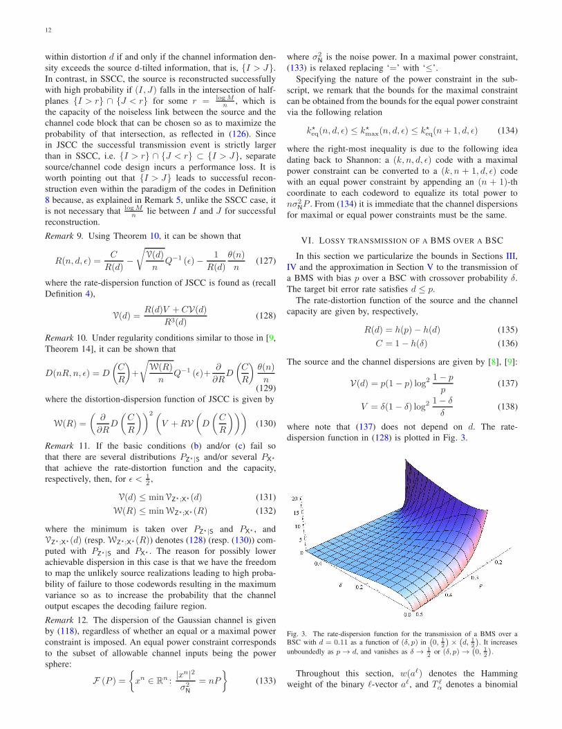
where note that (137) does not depend on d. The rate-

dispersion function in (128) is plotted in Fig. 3.

Fig. 3. The rate-dispersion function for the transmission of a BMS over aBSC with d = 0.11 as a function of (δ, p) in

(

0, 1

2

)

×

(

d, 1

2

)

. It increases

unboundedly as p → d, and vanishes as δ →1

2or (δ, p) →

(

0, 1

2

)

.

Throughout this section, w(aℓ) denotes the Hamming

weight of the binary ℓ-vector aℓ, and T ℓα denotes a binomial

13

random variable with parameters ℓ and α, independent of all

other random variables.

For convenience, we define the discrete random variable

Uα,β by

Uα,β =(T kα − kp

)log

1− p

p+(T nβ − nδ

)log

1− δ

δ(139)

In particular, substituting α = p and β = δ in (139), we

observe that the terms in the right side of (139) are zero-mean

random variables whose variances are equal to kV(d) and nV ,

respectively.

Furthermore, the binomial sum is denoted by

⟨k

ℓ

⟩=

ℓ∑

i=0

(k

i

)(140)

A straightforward particularization of the d-tilted informa-

tion converse in Theorem 2 leads to the following result.

Theorem 11 (Converse, BMS-BSC). Any (k, n, d, ǫ) code for

transmission of a BMS with bias p over a BSC with bias δmust satisfy

ǫ ≥ supγ≥0

{P [Up,δ ≥ nC − kR(d) + γ]− exp (−γ)

}(141)

Proof. Let PY n = PY n⋆ , which is the equiprobable distribu-

tion on {0, 1}n. An easy exercise reveals that

Sk(sk, d) = ıSk(sk)− kh(d) (142)

ıSk(sk) = kh(p) +(w(sk)− kp

)log

1− p

p(143)

ıXn;Y n⋆(xn; yn) = n (log 2− h(δ))

− (w(yn − xn)− nδ) log1− δ

δ(144)

Since w(Y n − xn) is distributed as T nδ regardless of xn ∈{0, 1}n, and w(Sk) is distributed as T kp , the condition in

Theorem 2 is satisfied, and (37) becomes (141).

The hypothesis-testing converse in Theorem 4 particularizes

to the following result:

Theorem 12 (Converse, BMS-BSC). Any (k, n, d, ǫ) code for

transmission of a BMS with bias p over a BSC with bias δmust satisfy

P

[U 1

2 ,12< r]+ λP

[U 1

2 ,12= r]≤⟨

k

⌊kd⌋

⟩2−k (145)

where 0 ≤ λ < 1 and scalar r are uniquely defined by

P [Up,δ < r] + λP [Up,δ = r] = 1− ǫ (146)

Proof. As in the proof of Theorem 11, we let PY n be the

equiprobable distribution on {0, 1}n, PY n = PY n⋆ . Since

under PY n|Xn=xn , w (Y n − xn) is distributed as T nδ , and

under PY n⋆ , w (Y n − xn) is distributed as T n12

, irrespective

of the choice of xn ∈ An, the distribution of the information

density in (144) does not depend on the choice of xn under

either measure, so Theorem 5 can be applied. Further, we

choose QSk to be the equiprobable distribution on {0, 1}k and

observe that under PSk , the random variable w(Sk) in (143)

has the same distribution as T kp , while under QSk it has the

same distribution as T k12

. Therefore, the log-likelihood ratio for

testing between PSkPY n|Xn=xn and QSkPY n⋆ has the same

distribution as (‘∼’ denotes equality in distribution)

logPSk(Sk)PY n|Xn=xn(Y n)

QSk(Sk)PY n⋆(Y n)

= ıXn;Y n⋆(xn;Y n)− ıSk(Sk) + k log 2 (147)

∼ n log 2− nh(δ)− kh(p)

−{Up,δ under PSkPY n|Xn=xn

U 12 ,

12

under QSkPY n⋆

(148)

so β1−ǫ(PSkPY n|Xn=xn , QSkPY n⋆) is equal to the left side

of (145). Finally, matching the size of the list to the fidelity

of reproduction using (55), we find that L is equal to the right

side of (145).

If the source is equiprobable, the bound in Theorem 12

becomes particularly simple, as the following result details.

Theorem 13 (Converse, EBMS-BSC). For p = 12 , if there

exists a (k, n, d, ǫ) joint source-channel code, then

λ

(n

r⋆ + 1

)+⟨ nr⋆

⟩≤⟨

k

⌊kd⌋

⟩2n−k (149)

where

r⋆ = max

{r :

r∑

t=0

(n

t

)δt(1 − δ)n−t ≤ 1− ǫ

}(150)

and λ ∈ [0, 1) is the solution to

r⋆∑

j=0

(n

t

)δt(1−δ)n−t+λδr⋆+1(1−δ)n−r⋆−1

(n

r⋆ + 1

)= 1−ǫ

(151)

The achievability result in Theorem 8 is particularized as

follows.

Theorem 14 (Achievability, BMS-BSC). There exists an

(k, n, d, ǫ) joint source-channel code with

ǫ ≤ infγ>0

{E

[exp

(− |U − log γ|+

)]+ e1−γ

}(152)

where

U = nC − (T nδ − nδ) log1− δ

δ− log

1

ρ(T kp )(153)

and ρ : {0, 1, . . . , k} 7→ [0, 1] is defined as

ρ(T ) =

k∑

t=0

L(T, t)qt(1 − q)k−t (154)

14

with

L(T, t) =

{(Tt0

)(k−Tt−t0

)t− kd ≤ T ≤ t+ kd

0 otherwise(155)

t0 =

⌈t+ T − kd

2

⌉+(156)

q =p− d

1− 2d(157)

Proof. We weaken the infima over PXn and PZk in (108)

by choosing them to be the product distributions generated

by the capacity-achieving channel input distribution and the

rate-distortion function-achieving reproduction distribution, re-

spectively, i.e. PXn is equiprobable on {0, 1}n, and PZk =PZ⋆ × . . .×PZ⋆ , where PZ⋆(1) = q. As shown in [9, proof of

Theorem 21],

PZk

(Bd(s

k))≥ ρ(w(sk)) (158)

On the other hand, |Y n−Xn|0 is distributed as T nδ , so (152)

follows by substituting (144) and (158) into (108).

In the special case of the BMS-BSC, Theorem 10 can be

strengthened as follows.

Theorem 15 (Gaussian approximation, BMS-BSC). The pa-

rameters of the optimal (k, n, d, ǫ) code satisfy (114) where

R(d), C, V(d), V are given by (135), (136), (137), (138),

respectively, and the remainder term in (114) satisfies

O (1) ≤ θ (n) (159)

≤ logn+ log logn+O (1) (160)

if 0 < d < p, and

−1

2logn+O (1) ≤ θ (n) (161)

≤ 1

2logn+O (1) (162)

if d = 0.

Proof. An asymptotic analysis of the converse bound in The-

orem 12 akin to that found in [9, proof of Theorem 23] leads

to (159) and (161). An asymptotic analysis of the achievability

bound in Theorem 14 similar to the one found in [9, Appendix

G] leads to (160). Finally, (162) is the same as (125).

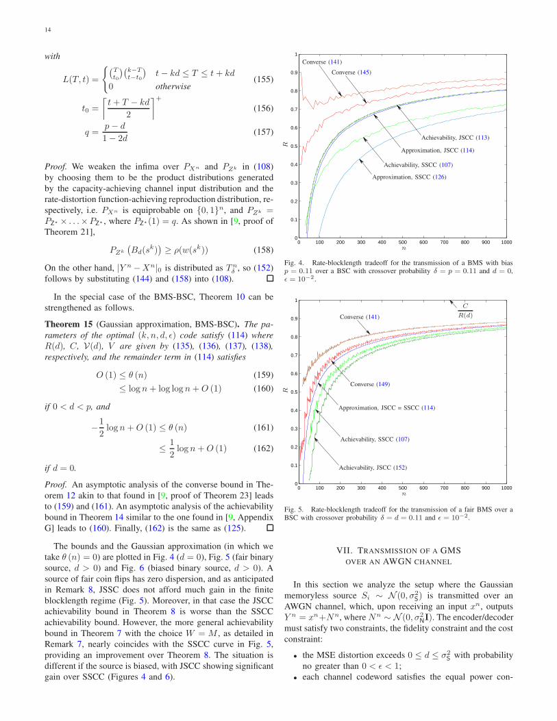
The bounds and the Gaussian approximation (in which we

take θ (n) = 0) are plotted in Fig. 4 (d = 0), Fig. 5 (fair binary

source, d > 0) and Fig. 6 (biased binary source, d > 0). A

source of fair coin flips has zero dispersion, and as anticipated

in Remark 8, JSSC does not afford much gain in the finite

blocklength regime (Fig. 5). Moreover, in that case the JSCC

achievability bound in Theorem 8 is worse than the SSCC

achievability bound. However, the more general achievability

bound in Theorem 7 with the choice W = M , as detailed in

Remark 7, nearly coincides with the SSCC curve in Fig. 5,

providing an improvement over Theorem 8. The situation is

different if the source is biased, with JSCC showing significant

gain over SSCC (Figures 4 and 6).

0 100 200 300 400 500 600 700 800 900 10000

0.1

0.2

0.3

0.4

0.5

0.6

0.7

0.8

0.9

1

n

R

Approximation, JSCC (114)

Converse (141)

Converse (145)

Approximation, SSCC (126)

Achievability, JSCC (113)

Achievability, SSCC (107)

Fig. 4. Rate-blocklength tradeoff for the transmission of a BMS with biasp = 0.11 over a BSC with crossover probability δ = p = 0.11 and d = 0,ǫ = 10−2 .

0 100 200 300 400 500 600 700 800 900 10000

0.1

0.2

0.3

0.4

0.5

0.6

0.7

0.8

0.9

1

n

R

C

R(d)



Converse (141)

Converse (149)

Approximation, JSCC = SSCC (114)

Fig. 5. Rate-blocklength tradeoff for the transmission of a fair BMS over aBSC with crossover probability δ = d = 0.11 and ǫ = 10−2.

VII. TRANSMISSION OF A GMS

OVER AN AWGN CHANNEL

In this section we analyze the setup where the Gaussian

memoryless source Si ∼ N (0, σ2S) is transmitted over an

AWGN channel, which, upon receiving an input xn, outputs

Y n = xn+Nn, where Nn ∼ N (0, σ2NI). The encoder/decoder

must satisfy two constraints, the fidelity constraint and the cost

constraint:

• the MSE distortion exceeds 0 ≤ d ≤ σ2S

with probability

no greater than 0 < ǫ < 1;

• each channel codeword satisfies the equal power con-

15

0 100 200 300 400 500 600 700 800 900 10000

0.5

1

1.5

2

n

R

C

R(d)Achievability, JSCC (152)


Converse (141)Converse (145)



Fig. 6. Rate-blocklength tradeoff for the transmission of a BMS with biasp = 0.11 over a BSC with crossover probability δ = p = 0.11 and d = 0.05,ǫ = 10−2.

straint in (133).7

The capacity-cost function and the rate-distortion function

are given by

R(d) =1

2log

(σ2S

d

)(163)

C(P ) =1

2log (1 + P ) (164)

The source dispersion is given by [9]:

V(d) = 1

2log2 e (165)

while the channel dispersion is given by (118) [8].

In the rest of the section, W ℓλ denotes a noncentral chi-

square distributed random variable with ℓ degrees of free-

dom and non-centrality parameter λ, independent of all other

random variables, and fW ℓλ

denotes its probability density

function.

A straightforward particularization of the d-tilted informa-

tion converse in Theorem 2 leads to the following result.

Theorem 16 (Converse, GMS-AWGN). If there exists a

(k, n, d, ǫ) code, then

ǫ ≥ supγ≥0

{P [U ≥ nC(P )− kR(d) + γ]− exp (−γ)

}

(166)

where

U =log e

2

(W k

0 − k)+

log e

2

(P

1 + PWn

nP− n

)(167)

7See Remark 12 in Section V for a discussion of the close relation betweenan equal and a maximal power constraint.

Observe that the terms to the left of the ‘≥’ sign inside the

probability in (166) are zero-mean random variables whose

variances are equal to kV(d) and nV , respectively.

Proof. The spherically-symmetric PY n = PY n⋆ = PY⋆ ×. . . × PY⋆ , where Y⋆ ∼ N (0, σ2

N(1 + P )) is the capacity-

achieving output distribution, satisfies the symmetry assump-

tion of Theorem 2. More precisely, it is not hard to show (see

[8, (205)]) that for all xn ∈ F(α), ıXn;Y n⋆(xn;Y n) has the

same distribution under PY n⋆|Xn=xn as

n

2log (1 + P )− log e

2

(P

1 + PWn

nP− n

)(168)

The d-tilted information in sk is given by

Sk(sk, d) =k

2log

σ2S

d+

( |sk|2σ2S

− k

)log e

2(169)

Plugging (168) and (169) into (37), (166) follows.

The hypothesis testing converse in Theorem 5 is particular-

ized as follows.

Theorem 17 (Converse, GMS-AWGN).

k

∫ ∞

0

rk−1P

[PWn

n(1+ 1P )

+ kd

σ2r2 ≤ nτ

]dr ≤ 1 (170)

where τ is the solution to

P

[P

1 + PWn

nP+W k

0 ≤ nτ

]= 1− ǫ (171)

Proof. As in the proof of Theorem 16, we let Y n ∼ Y n⋆ ∼N (0, σ2

N(1 + P )I). Under PY n|Xn=xn , the distribution of

ıXn;Y n⋆ (xn;Y n⋆) is that of (168), while under PY n⋆ , it has

the same distribution as (cf. [8, (204)])

n

2log(1 + P )− log e

2

(PWn

n(1+ 1P )

− n)

(172)

Since the distribution of ıXn;Y n⋆(xn;Y n⋆) does not depend on

the choice of xn ∈ Rn according to either measure, Theorem

5 applies. Further, choosing QSk to be the Lebesgue measure

on Rk, i.e. dQSk = dsk, observe that

log fSk(sk) = logdPSk(sk)

dsk= −k

2log(2πσ2

S

)− log e

2σ2S

|sk|2

(173)

Now, (170) and (171) are obtained by integrating

1

{log fSk(sk) + ıXn;Y n⋆(xn; yn) >

n

2log(1 + P ) +

n

2log e − k

2log(2πσ2

S)−log e

2nτ

}

(174)

with respect to dskdPY n⋆(yn) and dPSk(sk)dPY n|Xn=xn(yn),respectively.

The bound in Theorem 8 can be computed as follows.

16

Theorem 18 (Achievability, GMS-AWGN). There exists a

(k, n, d, ǫ) code such that

ǫ ≤ infγ>0

{E

[exp

{− |U − log γ|+

}]+ e1−γ

}(175)

where

U = nC(P )− log e

2

(P

1 + PWn

nP− n

)− log

F

ρ(W k0 )

(176)

F = maxn∈N,t∈R+

fWnnP

(t)

fWn0

(t

1+P

) <∞ (177)

and ρ : R+ 7→ [0, 1] is defined by

ρ(t) =Γ(k2 + 1

)√πkΓ

(k−12 + 1

)(1− L

(√t

k

)) k−12

(178)

where

L(r) =

0 r <√

dσ2S

−√1− d

σ2S

1∣∣∣r −

√1− d

σ2S

∣∣∣ >√

dσ2S(

1+r2−2 d

σ2S

)2

4

(1− d

σ2S

)r2

otherwise

(179)

Proof. We compute an upper bound to (108) for the specific

case of the transmission of a GMS over an AWGN chan-

nel. First, we weaken the infimum over PZk in (108) by

choosing PZk to be the uniform distribution on the surface

of the k-dimensional sphere with center at 0 and radius

r0 =√kσ√

1− dσ2S

. We showed in [9, proof of Theorem 37]

(see also [14], [22]) that

PZk

(Bd(s

k))≥ ρ

(|sk|2

)(180)

which takes care of the source random variable in (108).

We proceed to analyze the channel random variable

ıXn;Y n(Xn;Y n). Observe that since Xn lies on the power

sphere and the noise is spherically symmetric, |Y n|2 =|Xn +Nn|2 has the same distribution as |xn0 +Nn|2, where

xn0 is an arbitrary point on the surface of the power sphere.

Letting xn0 = σN√P (1, 1, . . . , 1), we see that 1

σN|xn0+Nn|2 =

∑ni=1

(1σ2N

Ni +√P)2

has the non-central chi-squared distri-

bution with n degrees of freedom and noncentrality parameter

nP . To simplify calculations, we express the information

density as

ıXn;Y n(xn0 ; yn) = ıXn;Y n⋆(xn0 ; y

n)− logdPY n

dPY n⋆

(yn) (181)

where Y n⋆ ∼ N (0, σ2N(1 + P )I). The distribution of

ıXn;Y n⋆(xn0 ;Yn) is the same as (168). Further, due to the

spherical symmetry of both PY n and PY n⋆ , as discussed

above, we have (recall that ‘∼’ denotes equality in distribution)

dPY n

dPY n⋆

(Y n) ∼fWn

nP(Wn

nP )

fWn0

(Wn

nP

1+P

) (182)

which is bounded uniformly in n as observed in [8, (425),

(435)], thus (177) is finite, and (175) follows.

The following result strengthens Theorem 10 in the special

case of the GMS-AWGN.

Theorem 19 (Gaussian approximation, GMS-AWGN). The

parameters of the optimal (k, n, d, ǫ) code satisfy (114) where

R(d), C, V(d), V are given by (163), (164), (165), (118),

respectively, and the remainder term in (114) satisfies

O (1) ≤ θ (n) (183)

≤ logn+ log logn+O (1) (184)

Proof. An asymptotic analysis of the converse bound in Theo-

rem 17 similar to that found in [9, proof of Theorem 40] leads

to (183). An asymptotic analysis of the achievability bound in

Theorem 18 similar to [9, Appendix K] leads to (184).

Numerical evaluation of the bounds reveals that JSCC

noticeably outperforms SSCC in the displayed region of

blocklengths (Fig. 7).

0 100 200 300 400 500 600 700 800 900 10000.2

0.3

0.4

0.5

0.6

0.7

0.8

0.9

1

n

R

C

R(d)


Converse (166)

Converse (170)




Fig. 7. Rate-blocklength tradeoff for the transmission of a GMS with d

σ2s=

0.5 over an AWGN channel with P = 1, ǫ = 10−2.

VIII. TO CODE OR NOT TO CODE

Our goal in this section is to compare the excess distor-

tion performance of the optimal code of rate 1 at channel

blocklength n with that of the optimal symbol-by-symbol

code, evaluated after n channel uses, leveraging the bounds

in Sections III and IV and the approximation in Section V.

We show certain examples in which symbol-by-symbol coding

is, in fact, either optimal or very close to being optimal.

A general conclusion drawn from this section is that even

when no coding is asymptotically suboptimal it can be a very

attractive choice for short blocklengths [2].

17

A. Performance of symbol-by-symbol source-channel codes

Definition 9. An (n, d, ǫ, α) symbol-by-symbol code is an

(n, n, d, ǫ, α) code (f, g) (according to Definition 2) that

satisfies

f(sn) = (f1(s1), . . . , f1(sn)) (185)

g(yn) = (g1(y1), . . . , g1(yn)) (186)

for some pair of functions f1 : S 7→ A and g1 : B 7→ S .

The minimum excess distortion achievable with symbol-by-

symbol codes at channel blocklength n, excess probability ǫand cost α is defined by

D1(n, ǫ, α) = inf {d : ∃(n, d, ǫ, α) symbol-by-symbol code} .(187)

Definition 10. The distortion-dispersion function of symbol-

by-symbol joint source-channel coding is defined as

W1(α) = limǫ→0

lim supn→∞

n (D (C(α)) −D1(n, ǫ, α))2

2 loge1ǫ

(188)

where D(·) is the distortion-rate function of the source.

As before, if there is no channel input-cost constraint

(cn(xn) = 0 for all xn ∈ An), we will simplify the notation

and write D1(n, ǫ) for D1(n, ǫ, α) and W1 for W1(α).

In addition to restrictions (i)–(iv) of Section V, we assume

that the channel and the source are probabilistically matched

in the following sense (cf. [7]).

(v) There exist α, PX⋆|S and PZ⋆|Y such that PX⋆ and PZ⋆|Sgenerated by the joint distribution PSPX⋆|SPY|XPZ⋆|Yachieve the capacity-cost function C(α) and the

distortion-rate function D (C(α)), respectively.

Condition (v) ensures that symbol-by-symbol transmission at-

tains the minimum average (over source realizations) distortion

achievable among all codes of any blocklength. The following

results pertain to the full distribution of the distortion incurred

at the receiver output and not just its mean.

Theorem 20 (Achievability, symbol-by-symbol code). Under

restrictions (i)-(v), if

P

[n∑

i=1

d(Si, Z⋆i ) > nd

]≤ ǫ (189)

where PZn⋆|Sn = PZ⋆|S × . . . × PZ⋆|S, and PZ⋆|S achieves

D (C(α)), then there exists an (n, d, ǫ, α) symbol-by-symbol

code (average cost constraint).

Proof. If (v) holds, then there exist a symbol-by-symbol

encoder and decoder such that the conditional distribution of

the output of the decoder given the source outcome coincides

with distribution PZ⋆|S, so the excess-distortion probability

of this symbol-by-symbol code is given by the left side of

(189).

Theorem 21 (Converse, symbol-by-symbol code). Under re-

striction (i) and separable distortion measure, the parameters

of any (n, d, ǫ, α) symbol-by-symbol code (average cost con-

straint) must satisfy

ǫ ≥ infPZ|S :

I(S;Z)≤C(α)

P

[n∑

i=1

d(Si, Zi) > nd

](190)

where PZn|Sn = PZ|S × . . .× PZ|S.

Proof. The excess-distortion probability at blocklength n, dis-

tortion d and cost α achievable among all single-letter codes(PX|S, PZ|Y

)must satisfy

ǫ ≥ infPX|S,PZ|Y :S−X−Y−Z

E[c(X)]≤α

P [dn(Sn, Zn) > d] (191)

≥ infPX|S,PZ|Y :

E[c(X)]≤αI(S;Z)≤I(X;Y)

P [dn(Sn, Zn) > d] (192)

where (192) holds since S − X − Y − Z implies I(S;Z) ≤I(X;Y) by the data processing inequality. The right side of

(192) is lower bounded by the right side of (190) because

I(X;Y) ≤ C(α) holds for all PX with E [c(X)] ≤ α, and the

distortion measure is separable.

Theorem 22 (Gaussian approximation, optimal symbol-

-by-symbol code). Assume E[d3 (S,Z⋆)

]< ∞. Under re-

strictions (i)-(v),

D1(n, ǫ, α) = D (C(α)) +

√W1(α)

nQ−1 (ǫ) +

θ1(n)

n(193)

W1(α) = Var [d(S,Z⋆)] (194)

where

θ1(n) ≤ O (1) (195)

Moreover, if there is no power constraint,

θ1(n) ≥D′(R)

R2θ(n) (196)

W1 = W(1) (197)

where θ(n) is that in Theorem 10.

If Var [d (S,Z⋆)] > 0 and S, S are finite, then

θ1(n) ≥ O (1) (198)

Proof. Since the third absolute moment of d(Si, Z⋆i ) is fi-

nite, the achievability part of the result, namely, (193) with

the remainder satisfying (195), follows by a straightforward

application of the Berry-Esseen bound to (189), provided that

Var [d(Si, Z⋆i )] > 0. If Var [d(Si, Z

⋆i )] = 0, it follows trivially

from (189).

To show the converse in (196), observe that since the set of

all (n, n, d, ǫ) codes includes all (n, d, ǫ) symbol-by-symbol

codes, we have D(n, n, ǫ) ≤ D1(n, ǫ). Since Q−1 (ǫ) is

positive or negative depending on whether ǫ < 12 or ǫ > 1

2 ,

using (130) we conclude that we must necessarily have (197),

which is, in fact, a consequence of conditions (b), (c) in

Section II and (v). Now, (196) is simply the converse part

of (129).

18

The proof of the refined converse in (198) is relegated to

Appendix E.

In the absence of a cost constraint, Theorem 22 shows that

if the source and the channel are probabilistically matched

in the sense of [7], then not only does symbol-by-symbol

transmission achieve the minimum average distortion, but also

the dispersion of JSCC (see (197)). In other words, not only

do such symbol-by-symbol codes attain the minimum average

distortion but also the variance of distortions at the decoder’s

output is the minimum achievable among all codes operating

at that average distortion. In contrast, if there is an average

cost constraint, the symbol-by-symbol codes considered in

Theorem 22 probably do not attain the minimum excess

distortion achievable among all blocklength-n codes, not even

asymptotically. Indeed, as observed in [23], for the trans-

mission of an equiprobable source over an AWGN channel

under the average power constraint and the average block error

probability performance criterion, the strong converse does not

hold and the second-order term is of order n− 13 , not n− 1

2 , as

in (193).

Two conspicuous examples that satisfy the probabilistic

matching condition (v), so that symbol-by-symbol coding is

optimal in terms of average distortion, are the transmission of a

binary equiprobable source over a binary-symmetric channel

provided the desired bit error rate is equal to the crossover

probability of the channel [24, Sec.11.8], [25, Problem 7.16],

and the transmission of a Gaussian source over an additive

white Gaussian noise channel under the mean-square error

distortion criterion, provided that the tolerable source signal-

to-noise ratio attainable by an estimator is equal to the signal-

to-noise ratio at the output of the channel [26]. We dissect

these two examples next. After that, we will discuss two

additional examples where uncoded transmission is optimal.

B. Uncoded transmission of a BMS over a BSC

In the setup of Section VI, if the binary source is unbiased(p = 1

2

), then C = 1−h(δ), R(d) = 1−h(d), and D(C) = δ.

If the encoder and the decoder are both identity mappings

(uncoded transmission), the resulting joint distribution satisfies

condition (v). As is well known, regardless of the blocklength,

the uncoded symbol-by-symbol scheme achieves the minimum

bit error rate (averaged over source and channel). Here, we

are interested instead in examining the excess distortion prob-

ability criterion. For example, consider an application where,

if the fraction of erroneously received bits exceeds a certain

threshold, then the entire output packet is useless.

Using (130) and (194), it is easy to verify that

W(1) = W1 = δ(1− δ) (199)

that is, uncoded transmission is optimal in terms of dispersion,

as anticipated in (197). Moreover, the uncoded transmission

attains the minimum bit error rate threshold D(n, n, ǫ) achiev-

able among all codes operating at blocklength n, regardless of

the allowed ǫ, as the following result demonstrates.

Theorem 23 (BMS-BSC, symbol-by-symbol code). Consider

the the symbol-by-symbol scheme which is uncoded if p ≥ δ

0 100 200 300 400 500 600 700 800 900 10000.1

0.15

0.2

0.25

0.3

0.35

0.4

0.45

0.5

n

d




No coding = converse (200)

Fig. 8. Distortion-blocklength tradeoff for the transmission of a fair BMSover a BSC with crossover probability δ = 0.11 and R = 1, ǫ = 10−2 .

and whose decoder always outputs the all-zero vector if p < δ.

It achieves, at blocklength n and excess distortion probability

ǫ, regardless of 0 ≤ p ≤ 12 , δ ≤ 1

2 ,

D1(n, ǫ) =

min

d :

⌊nd⌋∑

t=0

(n

t

)min{p, δ}t(1−min{p, δ})n−t ≥ 1− ǫ

(200)

Moreover, if the source is equiprobable(p = 1

2

),

D1(n, ǫ) = D(n, n, ǫ) (201)

Proof. Direct calculation yields (200). To show (201), let us

compare d⋆ = D1(n, ǫ) with the conditions imposed on d by

Theorem 13. Comparing (200) to (150), we see that either

(a) equality in (200) is achieved, r⋆ = nd⋆, λ = 0, and

(plugging k = n into (149))

⟨ n

nd⋆

⟩≤⟨

n

⌊nd⌋

⟩(202)

thereby implying that d ≥ d⋆, or

(b) r⋆ = nd⋆ − 1, λ > 0, and (149) becomes

λ

(n

nd⋆

)+

⟨n

nd⋆ − 1

⟩≤⟨

n

⌊nd⌋

⟩(203)

which also implies d ≥ d⋆. To see this, note that d < d⋆

would imply ⌊nd⌋ ≤ nd⋆−1 since nd⋆ is an integer, which

in turn would require (according to (203)) that λ ≤ 0,

which is impossible.

For the transmission of the fair binary source over a BSC,

Fig. 8 shows the distortion achieved by the uncoded scheme,

the separated scheme and the JSCC scheme of Theorem 14

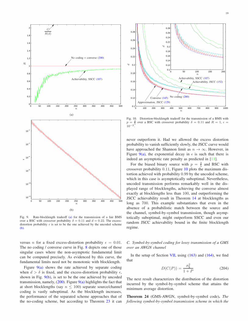
19

0 50 100 150 200 250 300 350 400 450 5000

0.2

0.4

0.6

0.8

1

1.2

1.4

1.6

1.8

2

n

R

C

R(d)


No coding = converse (200)

(a)

0 50 100 150 200 250 300 350 400 450 500

10−12

10−10

10−8

10−6

10−4

10−2

ε

n

(b)

Fig. 9. Rate-blocklength tradeoff (a) for the transmission of a fair BMSover a BSC with crossover probability δ = 0.11 and d = 0.22. The excess-distortion probability ǫ is set to be the one achieved by the uncoded scheme(b).

versus n for a fixed excess-distortion probability ǫ = 0.01.

The no coding / converse curve in Fig. 8 depicts one of those

singular cases where the non-asymptotic fundamental limit

can be computed precisely. As evidenced by this curve, the

fundamental limits need not be monotonic with blocklength.

Figure 9(a) shows the rate achieved by separate coding

when d > δ is fixed, and the excess-distortion probability ǫ,shown in Fig. 9(b), is set to be the one achieved by uncoded

transmission, namely, (200). Figure 9(a) highlights the fact that

at short blocklengths (say n ≤ 100) separate source/channel

coding is vastly suboptimal. As the blocklength increases,

the performance of the separated scheme approaches that of

the no-coding scheme, but according to Theorem 23 it can

0 100 200 300 400 500 600 700 800 900 10000.1

0.12

0.14

0.16

0.18

0.2

0.22

0.24

0.26

0.28

0 50 100 150 2000.1

0.12

0.14

0.16

0.18

0.2

0.22

0.24

0.26

0.28

n

n

d

d



Converse (145)


No coding (200)

Fig. 10. Distortion-blocklength tradeoff for the transmission of a BMS withp = 2

5over a BSC with crossover probability δ = 0.11 and R = 1, ǫ =

10−2.

never outperform it. Had we allowed the excess distortion

probability to vanish sufficiently slowly, the JSCC curve would

have approached the Shannon limit as n → ∞. However, in

Figure 9(a), the exponential decay in ǫ is such that there is

indeed an asymptotic rate penalty as predicted in [11].

For the biased binary source with p = 25 and BSC with

crossover probability 0.11, Figure 10 plots the maximum dis-

tortion achieved with probability 0.99 by the uncoded scheme,

which in this case is asymptotically suboptimal. Nevertheless,

uncoded transmission performs remarkably well in the dis-

played range of blocklengths, achieving the converse almost

exactly at blocklengths less than 100, and outperforming the

JSCC achievability result in Theorem 14 at blocklengths as

long as 700. This example substantiates that even in the

absence of a probabilistic match between the source and

the channel, symbol-by-symbol transmission, though asymp-

totically suboptimal, might outperform SSCC and even our

random JSCC achievability bound in the finite blocklength

regime.

C. Symbol-by-symbol coding for lossy transmission of a GMS

over an AWGN channel

In the setup of Section VII, using (163) and (164), we find

that

D(C(P )) =σ2S

1 + P(204)

The next result characterizes the distribution of the distortion

incurred by the symbol-by-symbol scheme that attains the

minimum average distortion.

Theorem 24 (GMS-AWGN, symbol-by-symbol code). The

following symbol-by-symbol transmission scheme in which the

20

encoder and the decoder are the amplifiers:

f1(s) = as, a2 =Pσ2

N

σ2S

(205)

g1(y) = by, b =aσ2

S

a2σ2S+ σ2

N

(206)

is an (n, d, ǫ, P ) symbol-by-symbol code (with average cost

constraint) such that

P [Wn0 D(C(P )) > nd] = ǫ (207)

where Wn0 is chi-square distributed with n degrees of freedom.

Note that (207) is a particularization of (189). Using (207),

we find that

W1(P ) = 2σ4S

(1 + P )2 (208)

On the other hand, using (130), we compute

W(1, P ) = 2σ4S

(1 + P )2

(2− 1

(1 + P )2

)(209)

>W1(P ) (210)

The difference between (210) and (197) is due to the fact that

the optimal symbol-by-symbol code in Theorem 24 obeys an

average power constraint, rather than the more stringent max-

imal power constraint of Theorem 10, so it is not surprising

that for the practically interesting case ǫ < 12 the symbol-

by-symbol code can outperform the best code obeying the

maximal power constraint. Indeed, in the range of blocklenghts

displayed in Figure 11, the symbol-by-symbol code even

outperforms the converse for codes operating under a maximal

power constraint.

0 100 200 300 400 500 600 700 800 900 10000.5

0.55

0.6

0.65

0.7

0.75

0.8

n

d


Converse (170)



No coding (207)

Approximation, no coding (194)

Fig. 11. Distortion-blocklength tradeoff for the transmission of a GMS overan AWGN channel with P

σ2N

= 1 and R = 1, ǫ = 10−2.

D. Uncoded transmission of a discrete memoryless source

(DMS) over a discrete erasure channel (DEC) under erasure

distortion measure

For a discrete source, the single-letter erasure distortion

measure is defined as the following mapping d : S×{S, e} 7→[0,∞]:8

d(s, z) =

0 z = s

H(S) z = e

∞ otherwise

(211)

For any 0 ≤ d ≤ H(S), the rate-distortion function of the

equiprobable source is achieved by

PZ⋆|S=s(z) =

{1− d

H(S) z = sd

H(S) z = e(212)

The rate-distortion function and the d-tilted information for

the equiprobable source with the erasure distortion measure

are given by, respectively,

R(d) = H(S)− d (213)

S(s, d) = ıS(s)− d (214)

Note that, trivially, S(S, d) = R(d) = log |S| − d a.s. The

channel that is matched to the equiprobable DMS with the

erasure distortion measure is the DEC, whose single-letter

transition probability kernel PY|X : A 7→ {A, e} is

PY|X=x(y) =

{1− δ y = x

δ y = e(215)

and whose capacity is given by C = log |A| − δ, achieved by

equiprobable PX⋆ . For PS equiprobable on S = A, we find

that D(C) = δ log |S|, and

W1 = δ (1− δ) log2 |S| (216)

E. Symbol-by-symbol transmission of a DMS over a DEC

under logarithmic loss

Let the source alphabet S be finite, and let the reproduction

alphabet S be the set of all probability distributions on S. The

single-letter logarithmic loss distortion measure d : S × S 7→R+ is defined by [28], [29]

d(s, PZ) = ıZ(s) (217)

Curiously, for any 0 ≤ d ≤ H(S), the rate-distortion

function and the d-tilted information are given respectively

by (213) and (214), even if the source is not equiprobable. In

fact, the rate-distortion function is achieved by,

PP⋆Z|S=s(PZ) =

{d

H(S) PZ = PS

1− dH(S) PZ = 1S(s)

(218)

and the channel that is matched to the equiprobable source

under logarithmic loss is exactly the DEC in (215). Of course,

unlike Section VIII-D, the decoder we need is a simple one-

to-one function that outputs PS if the channel output is e, and

8The distortion measure in (211) is a scaled version of the erasure distortionmeasure found in literature, e.g. [27].

21

1S(y) otherwise, where y 6= e is the output of the DEC. Finally,

it is easy to verify that the distortion-dispersion function of

symbol-by-symbol coding under logarithmic loss is the same

as that under erasure distortion and is given by (216).

IX. CONCLUSION

In this paper we gave a non-asymptotic analysis of joint

source-channel coding including several achievability and con-

verse bounds, which hold in wide generality and are tight

enough to determine the dispersion of joint source-channel

coding for the transmission of an abstract memoryless source

over either a DMC or a Gaussian channel, under an arbitrary

fidelity measure. We also investigated the penalty incurred by

separate source-channel coding using both the source-channel

dispersion and the particularization of our new bounds to

(i) the binary source and the binary symmetric channel with

bit error rate fidelity criterion and (ii) the Gaussian source

and Gaussian channel under mean-square error distortion.

Finally, we showed cases where symbol-by-symbol (uncoded)

transmission beats any other known scheme in the finite

blocklength regime even when the source-channel matching

condition is not satisfied.

The approach taken in this paper to analyze the non-

asymptotic fundamental limits of lossy joint source-channel

coding is two-fold. Our new achievability and converse bounds

apply to abstract sources and channels and allow for memory,

while the asymptotic analysis of the new bounds leading to the

dispersion of JSCC is focused on the most basic scenario of

transmitting a stationary memoryless source over a stationary

memoryless channel.

The major results and conclusions are the following.

1) A general new converse bound (Theorem 3) leverages the

concept of d-tilted information (Definition 5), a random

variable which corresponds (in a sense that can be formal-

ized [9], [30]) to the number of bits required to represent

a given source outcome within distortion d and whose role

in lossy compression is on a par with that of information

(in (20)) in lossless compression.

2) The converse result in Theorem 4 capitalizes on two

simple observations, namely, that any (d, ǫ) lossy code can

be converted to a list code with list error probability ǫ,and that a binary hypothesis test between PSXY and an

auxiliary distribution on the same space can be constructed

by choosing PSXY when there is no list error. We have

generalized the conventional notion of list, to allow the

decoder to output a possibly uncountable set of source

realizations.

3) As evidenced by our numerical results, the converse result

in Theorem 5, which applies to those channels satisfying a

certain symmetry condition and which is a consequence

of the hypothesis testing converse in Theorem 4, can

outperform the d-tilted information converse in Theorem

3. Nevertheless, it is Theorem 3 that lends itself to analysis

more easily and that leads to the JSCC dispersion for the

general DMC.

4) Our random-coding-based achievability bound (Theorem 7)

provides insights into the degree of separation between the

source and the channel codes required for optimal perfor-

mance in the finite blocklength regime. More precisely,

it reveals that the dispersion of JSCC can be achieved

in the class of (M,d, ǫ) JSCC codes (Definition 8). As

in separate source/channel coding, in (M,d, ǫ) coding the

inner channel coding block is connected to the outer source

coding block by a noiseless link of capacity logM , but

unlike SSCC, the channel (resp. source) code can be chosen

based on the knowledge of the source (resp. channel). The

conventional SSCC in which the source code is chosen

without knowledge of the channel and the channel code is

chosen without knowledge of the source, although known

to achieve the asymptotic fundamental limit of joint source-

channel coding under certain quite weak conditions, is in

general suboptimal in the finite blocklength regime.

5) Since E [d(S,Z)] =∫∞0 P [d(S,Z) > ξ] dξ, bounds for

average distortion can be obtained by integrating our

bounds on excess distortion. Note, however, that the code

that minimizes P [d(S,Z) > ξ] depends on ξ. Since the

distortion cdf of any single code does not majorize the

cdfs of all possible codes, the converse bound on the

average distortion obtained through this approach, although

asymptotically tight, may be loose at short blocklengths.

Likewise, regarding achievability bounds (e.g. (108)), the

optimization over channel and source random codes, PXand PZ , must be performed after the integration, so that the

choice of code does not depend on the distortion threshold

ξ.

6) For the transmission of a stationary memoryless source

over a stationary memoryless channel, the Gaussian ap-

proximation in Theorem 10 (neglecting the remainder

θ(n)) provides a simple estimate of the maximal non-

asymptotically achievable joint source-channel coding rate.

Appealingly, the dispersion of joint source-channel coding

decomposes into two terms, the channel dispersion and

the source dispersion. Thus, only two channel attributes,

the capacity and dispersion, and two source attributes, the

rate-distortion and rate-dispersion functions, are required to

compute the Gaussian approximation to the maximal JSCC

rate.

7) In those curious cases where the source and the channel are

probabilistically matched so that symbol-by-symbol coding

attains the minimum possible average distortion, Theorem

22 ensures that it also attains the dispersion of joint source-

channel coding, that is, symbol-by-symbol coding results

in the minimum variance of distortions among all codes

operating at that average distortion.

8) Even in the absence of a probabilistic match between

the source and the channel, symbol-by-symbol transmis-

sion, though asymptotically suboptimal, might outperform

separate source-channel coding and joint source-channel

random coding in the finite blocklength regime.

ACKNOWLEDGEMENT

The authors are grateful to Dr. Oliver Kosut for offering

numerous comments, and, in particular, suggesting the sim-

plification of the achievability bound in [1] with the tighter

version in Theorem 8.

22

APPENDIX A

THE BERRY-ESSEEN THEOREM

The following result is an important tool in the Gaussian

approximation analysis.

Theorem 25 (Berry-Esseen CLT, e.g. [31, Ch. XVI.5 Theorem

2]). Fix a positive integer n. Let Wi, i = 1, . . . , n be

independent. Then, for any real t∣∣∣∣∣P[

n∑

i=1

Wi > n

(Dn + t

√Vnn

)]−Q(t)

∣∣∣∣∣ ≤Bn√n, (219)

where

Dn =1

n

n∑

i=1

E [Wi] (220)

Vn =1

n

n∑

i=1

Var [Wi] (221)

Tn =1

n

n∑

i=1

E[|Wi − E [Wi] |3

](222)

Bn =c0Tn

V3/2n

(223)

and 0.4097 ≤ c0 ≤ 0.5600 (0.4097 ≤ c0 < 0.4784 for

identically distributed Wi).

APPENDIX B

AUXILIARY RESULT ON THE MINIMIZATION OF THE

INFORMATION SPECTRUM

Given a finite set A, we say that xn ∈ An has type PX if

the number of times each letter a ∈ A is encountered in xn is

nPX(a). Let P be the set of all distributions on A, which is

simply the standard |A| − 1 simplex in R|A|. For an arbitrary

subset D ⊆ P , denote by D[n] the set of distributions in Dthat are also n-types, that is,

D[n] = {PX ∈ D : ∀a ∈ A, nPX(a) is an integer} (224)

Denote by Π(PX) the minimum Euclidean distance approxi-

mation of PX ∈ P in the set of n-types, that is,

Π(PX) = arg minPX∈P[n]

∣∣∣PX − PX

∣∣∣ (225)

Let P⋆ be the set of capacity-achieving distributions:9

P⋆ = {PX ∈ P : I(X;Y) = C} (226)

Denote the minimum (maximum) information variances

achieved by the distributions in P⋆ by

Vmin = minPX∈P⋆

Var [ıX;Y(X;Y)] (227)

Vmax = maxPX∈P⋆

Var [ıX;Y(X;Y)] (228)

and let P⋆min ⊆ P⋆ be the set of capacity-achieving distribu-

tions that achieve the minimum information variance:

P⋆min = {PX ∈ P⋆ : Var [ıX;Y(X;Y)] = Vmin} (229)

9In this appendix, we dispose of the assumption (c) in Section II that thecapacity-achieving input distribution is unique.

and analogously P⋆max for the distributions in P⋆ with max-

imal variance. Lemma 1 below allows to show that in the

memoryless case, the infimum inside the expectation in (39)

with W = type (Xn) and PY n|W=PX= PY × . . . × PY,

where PY is the output distribution induced by the type PX,

is approximately attained by those sequences whose type is

closest to the capacity-achieving distribution PX⋆ (if it is non-

unique, PX⋆ is chosen appropriately based on the information

variance it achieves). This technical result is the key to proving

the converse part of Theorem 10.

Lemma 1. There exist ∆ > 0 such that for all sufficiently

large n:

1) If Vmin > 0, then there exists K > 0 such that for |∆| ≤∆,

minxn∈An

P

[n∑

i=1

ıX;Y(xi;Yi) ≤ n (C −∆)

]

≥ P

[n∑

i=1

ıX;Y(x⋆i ;Yi) ≤ n (C −∆)

]− K√

n(230)

where (230) holds for any xn⋆ with type(xn⋆) = Π(P ⋆X)

for P ⋆X∈ P⋆min if ∆ ≥ 0 and P ⋆

X∈ P⋆max if ∆ < 0.

2) If Vmax = 0, then for all 0 < α < 32 and ∆ ≥ ∆

n12+α

,

minxn∈An

P

[n∑

i=1

ıX;Y(xi;Yi) ≤ n (C +∆)

]≥ 1− 1

n14− 3

2α

(231)

The information densities in the left sides of (230) and (231)

are computed with{PY|X=xi

, PY

}, where PY is induced by

the type of xn, i.e. type(xn) = PX → PY|X → PY, and that

in the right side of (230) is computed with{PY|X=x⋆

i, PY

},

where PY is induced by the type of xn⋆, i.e. type(xn⋆) =PX → PY|X → PY. The independent random variables Yi in

the left sides of (230) and (231) have distribution PY|X=xi,

while Yi in the right side of (230) have distribution PY|X=x⋆i.

In order to prove Lemma 1, we first show three auxiliary

lemmas. The first two deal with approximate optimization of

functions.

If f and g approximate each other, and the minimum of fis approximately attained at x, then g is also approximately

minimized at x, as the following lemma formalizes.

Lemma 2. Fix η > 0, ξ > 0. Let D be an arbitrary set, and

let f : D 7→ R and g : D 7→ R be such that

supx∈D

|f(x)− g(x)| ≤ η (232)

Further, assume that f and g attain their minima. Then,

g(x) ≤ miny∈D

g(y) + ξ + 2η (233)

as long as x satisfies

f(x) ≤ miny∈D

f(y) + ξ (234)

(see Fig. 12).

23

x

f

g

η

η

ξ

erse (

Fig. 12. An example where (233) holds with equality.

Proof of Lemma 2. Let x⋆ ∈ D be such that g(x⋆) =miny∈D g(y). Using (232) and (234), write

g(x) ≤ miny∈D

f(y) + g(x) − f(x) + ξ (235)

≤ miny∈D

f(y) + η + ξ (236)

≤ f(x⋆) + η + ξ (237)

= g(x⋆)− g(x⋆) + f(x⋆) + η + ξ (238)

≤ g(x⋆) + 2η + ξ (239)

The following lemma is reminiscent of [8, Lemma 64].

Lemma 3. Let D be a compact metric space, and let d : D2 →R+ be a metric. Fix f : D 7→ R and g : D 7→ R. Let

D⋆ =

{x ∈ D : f(x) = max

y∈Df(y)

}(240)

Suppose that for some constants ℓ > 0, L > 0, we have, for

all (x, x⋆) ∈ D ×D⋆,

f(x⋆)− f(x) ≥ ℓd2(x, x⋆) (241)

|g(x⋆)− g(x)| ≤ Ld(x, x⋆) (242)

Then, for any positive scalars ϕ, ψ,

maxx∈D

{ϕf(x)± ψg(x)} ≤ ϕf(x⋆)± ψg(x⋆) +L2ψ2

4ℓϕ(243)

Moreover, if, instead of (241), f satisfies

f(x⋆)− f(x) ≥ ℓd(x, x⋆) (244)

then, for any positive scalars ψ, ϕ such that

Lψ ≤ ℓϕ (245)

we have

maxx∈D

{ϕf(x)± ψg(x)} = ϕf(x⋆)± ψg(x⋆) (246)

Proof of Lemma 3. Let x0 achieve the maximum on the left

side of (243). Using (241) and (242), we have, for all x⋆ ∈ D⋆,

0 ≤ ϕ (f(x0)− f(x⋆))± ψ (g(x0)− g(x⋆)) (247)

≤ −ℓϕd2(x0, x⋆) + Lψd(x0, x⋆) (248)

≤ L2ψ2

4ℓϕ(249)

where (249) follows because the maximum of (248) is

achieved at d(x0, x⋆) = Lψ

2ℓϕ .

To show (246), observe using (244) and (242) that

0 ≤ ϕ (f(x0)− f(x⋆))± ψ (g(x0)− g(x⋆)) (250)

≤ (−ℓϕ+ Lψ) d(x0, x⋆) (251)

≤ 0 (252)

where (252) follows from (245).

The following lemma deals with asymptotic behavior of the

Q-function.

Lemma 4. Fix a ≥ 0, b ≥ 0. Then, there exists q ≥ 0(explicitly computed in the proof) such that for all z ≥ −

√n

2band all n large enough,

Q

(z − a√

n

)−Q

(z +

b√nz2)

≤ q√n

(253)

Proof of Lemma 4. Q(x) is convex for x ≥ 0, and Q′(x) =

− 1√2πe−

x2

2 , so for x ≥ 0, ξ ≥ 0

Q(x+ ξ) ≥ Q(x)− ξ√2πe−

x2

2 (254)

while for arbitrary x and ξ ≥ 0,

Q(x+ ξ) ≥ Q(x)− ξ√2π

(255)

If z ≥ a√n

, we use (254) to obtain

Q

(z − a√

n

)−Q

(z +

b√nz2)

(256)

≤ 1√2πe−

(z− a√

n

)2

2

(b√nz2 +

a√n

)(257)

≤ bz2√2πn

e−

(z− a√

n

)2

2 +a√2πn

(258)

≤ 3b e−1 + a√2πn

(259)

where (259) holds for n large enough because the maximum

of (258) is attained at z =√2 + a

4n + a2√n

.

If 0 ≤ z ≤ a√n

, we use (255) to obtain

Q

(z − a√

n

)−Q

(z +

b√nz2)

≤ 1√2π

(b√nz2 +

a√n

)(260)

≤ a√2πn

(1 +

ab

n

)(261)

24

If −√n

2b ≤ z ≤ 0, we use Q(x) = 1−Q(−x) to obtain

Q

(z − a√

n

)−Q

(z +

b√nz2)

= Q

(|z| − b√

nz2)−Q

(|z|+ a√

n

)(262)

≤ 1√2πe−

z2(1− b√

n|z|

)2

2

(b√nz2 +

a√n

)(263)

≤ bz2√2πn

e−z2

(1− b√

n|z|

)2

2 +a√2πn

(264)

≤ bz2√2πn

e−z2

8 +a√2πn

(265)

≤ 8be−1 + a√2πn

(266)

where (265) is due to(1− b√

n|z|)2

≥ 14 in |z| ≤

√n

2b , and

(266) holds because the maximum of (265) is attained at z2 =8.

We are now equipped to prove Lemma 1.

Proof of Lemma 1. Define the following functions P 7→ R+:

I(PX) = I(X;Y) = E [ıX;Y(X;Y)] (267)

V (PX) = E [Var [ıX;Y(X;Y) | X]] (268)

T (PX) = E

[|ıX;Y(X;Y) − E [ıX;Y(X;Y)|X]|3 | X

](269)

If PX = type(xn), then for each a ∈ A, there are nPX(a) oc-

currences of PY|X=a among the {PY|X=xi, i = 1, 2, . . . , n}. In

the sequel we will invoke Theorem 25 with Wi = ıX;Y(xi;Yi)where xn is a given sequence, and (220)–(222) become

Dn =1

n

|A|∑

a=1

nPX(a)E [ıX;Y(a;Y) | X = a] (270)

= I(PX) (271)

Vn =1

n

|A|∑

a=1

nPX(a)Var [ıX;Y(a;Y) | X = a]

(272)

= V (PX) (273)

Tn =1

n

|A|∑

a=1

nPX(a) |ıX;Y(a;Y)− E [ıX;Y(a;Y)|X = a]|3

= T (PX) (274)

Define the (Euclidean) δ-neighborhood of the set of

capacity-achieving distributions P⋆,

P⋆δ =

{PX ∈ P : min

PX⋆∈P⋆|PX − PX⋆ | ≤ δ

}(275)

We split the domain of the minimization in the left side

of (230) into two sets, type(xn) ∈ P⋆δ,[n] and type(xn) ∈P[n]\P⋆δ (recall notation (224)), for an appropriately chosen

δ > 0.

We now show that (230) holds for all ∆ ≤ ∆I

2 if the

minimization is restricted to types in P[n]\P⋆δ , where δ > 0

is arbitrary, and

∆I = C − maxPX∈P[n]\P⋆

δ

I(PX) > 0 (276)

By Chebyshev’s inequality, for all xn whose type belongs to

P[n]\P⋆δ ,

P

[n∑

i=1

ıX;Y(xi;Yi) > n(C −∆)

](277)

= P

[n∑

i=1

ıX;Y(xi;Yi)− nI(PX) > n(C − I(PX))− n∆

]

(278)

≤ P

[n∑

i=1

ıX;Y(xi;Yi)− nI(PX) >n∆I

2

](279)

≤ P

(

n∑

i=1

ıX;Y(xi;Yi)− nI(PX)

)2

>n2∆2

I

4

(280)

≤ 4nV (PX)

n2∆2I

(281)

≤ 4V

n∆2I

(282)

where in (279) we used

∆ ≤ 1

2∆I < ∆I ≤ C − I(PX) (283)

and

V = maxPX∈P

V (PX) (284)

Note that V <∞ by Property 1 below. Therefore,

mintype(xn)∈P[n]\P⋆

δ

P

[n∑

i=1

ıX;Y(xi;Yi) ≤ n(C −∆)

](285)

> 1− 4V

n∆2I

(286)

≥ P

[n∑

i=1

ıX;Y(x⋆i ;Yi) ≤ n(C −∆)

]− 4V

n∆2I

(287)

We conclude that (230) holds if the minimization is restricted

to types in P[n]\P⋆δ .

Without loss of generality, we assume that all outputs in Bare accessible (which implies that PY⋆(y) > 0 for all y ∈ B)

and choose δ > 0 so that for all PX ∈ P⋆δ and y ∈ B,

PY(y) > 0 (288)

where PX → PY|X → PY. We recall the following properties

of the functions I(·), V (·) and T (·) from [8, Appendices E

and I].

Property 1. The functions I(PX), V (PX) and T (PX) are

continuous on the compact set P , and therefore bounded and

achieve their extrema.

Property 2. There exists ℓ1 > 0 such that for all (PX⋆ , PX) ∈P⋆ × P⋆δ ,

C − I(PX) ≥ ℓ1 |PX − PX⋆ |2 (289)

25

Property 3. In P⋆δ , the functions I(PX), V (PX) and T (PX)are infinitely differentiable.

Property 4. In P⋆, V (PX) = Var [ıX;Y(X;Y)].

Due to Property 3, there exist nonnegative constants L1 and

L2 such that for all (PX, PX⋆) ∈ P⋆δ × P⋆,

C − I(PX) ≤ L1 |PX − PX⋆ | (290)

|V (PX)− V (PX⋆)| ≤ L2 |PX − PX⋆ | (291)

To treat the case xn ∈ P⋆δ,[n], we will need to choose δ > 0carefully and to consider the cases Vmin > 0 and Vmax = 0separately.

A. Vmin > 0.

We decrease δ until, in addition to (288),

Vmin ≤ 2 minPX∈P⋆

δ

V (PX) (292)

is satisfied.

We now show that (230) holds if the minimization is

restricted to types in P⋆δ,[n], for all −∆ ≤ ∆ ≤ ∆I

2 , for

an appropriately chosen ∆ > 0. Using (292) and boundedness

of T (PX), write

B = maxPX∈P⋆

δ

c0T (PX)

V32 (PX)

≤ 232 c0T

V32

min

<∞ (293)

where

T = maxPX∈P⋆

δ

T (PX) <∞ (294)

Therefore, for any xn with type(xn) ∈ P⋆δ,[n], the Berry-

Esseen bound yields:

∣∣∣∣∣P[n∑

i=1


]−Q (ν(PX))

∣∣∣∣∣ ≤B√n

(295)

where

ν(PX) =nI(PX)− nC + n∆√

nV (PX)(296)

We now apply Lemma 2 with D = P⋆δ,[n] and

f(PX) = Q (ν(PX)) (297)

g(PX) = P

[n∑

i=1


](298)

Condition (232) of Lemma 2 holds with η = B√n

due to

(295). As will be shown in the sequel, the following version

of condition (234) holds:

Q(ν(Π(PX⋆))) ≤ minPX∈P⋆

δ,[n]

Q(ν(PX)) +q√n

(299)

where Π(PX⋆), the minimum Euclidean distance approxima-

tion of PX⋆ in the set of n-types, is formally defined in (225),

and q > 0 will be chosen later. Applying Lemma 2, we deduce

from (233) that

mintype(xn)∈P⋆

δ,[n]

P

[n∑

i=1


]

≥ P

[n∑

i=1

ıX;Y(x⋆i ;Yi) ≤ n(C −∆)

]− q + 2B√

n

(300)

We conclude that (230) holds if minimization is restricted to

types in P⋆δ,[n].We proceed to show (299). As will be proven later, for

appropriately chosen L > 0 and L > 0 we can write

√n∆√

V (PX⋆)− L√

n

√|A|(|A| − 1) ≤ ν(Π (PX⋆)) (301)

≤ maxPX∈P⋆

δ,[n]

ν(PX) (302)

≤ maxPX∈P⋆

δ

ν(PX) (303)

≤√n∆√

V (PX⋆)+√nL∆2

(304)

where PX⋆ ∈ P⋆min if ∆ ≥ 0, and PX⋆ ∈ P⋆max if ∆ < 0.

Denote

a = L√|A| (|A| − 1) (305)

b = V (PX⋆)L (306)

z =

√n∆√

V (PX⋆)(307)

If

∆ ≥ − 1

2L√Vmax

= −∆ (308)

then z ≥ −√n

2b , and Lemma 4 applies to z. So, using (301),

(304), the fact that Q(·) is monotonically decreasing and

Lemma 4, we conclude that there exists q > 0 such that

Q (ν(Π(PX⋆))) − minPX∈P⋆

δ,[n]

Q(ν(PX))

= Q (ν(Π(PX⋆))) −Q

(max

PX∈P⋆δ,[n]

ν(PX)

)(309)

≤ Q

(z − a√

n

)−Q

(z +

b√nz2)

(310)

≤ q√n

(311)

which is equivalent to (299).

It remains to prove (301) and (304). Observing that for

a, b > 0∣∣∣∣1√a− 1√

b

∣∣∣∣ =|a− b|

√a√b(√

a+√b) (312)

≤ |a− b|2min {a, b} 3

2

(313)

26

and using (291) and (292), we have, for all (PX, PX⋆) ∈ P⋆δ ×P⋆,

∣∣∣∣∣1√V (PX)

− 1√V (PX⋆)

∣∣∣∣∣ ≤ L |PX − PX⋆ | (314)

where

L = L2

√2

V 3min

(315)

Thus, recalling (290) and denoting ζ = |PX − PX⋆ |, we have

C − I(PX)−∆√V (PX)

≤ L1ζ −∆√V (PX)

(316)

≤ L1ζ −∆√V (PX⋆)

+ Lζ (L1ζ + |∆|) (317)

≤ − ∆√V (PX⋆)

+ Lζ (318)

where

L =L1√Vmin

+ Lmax

{∆,

∆I

2

}+ LL1δ (319)

So, (301) follows by observing that for any PX ∈ P ,

|PX −Π(PX)| ≤1

n

√|A|(|A| − 1) (320)

and letting PX = Π(PX⋆) in (316)–(318).

To show (304), we apply Lemma 3 with

D = P⋆δ (321)

D⋆ = P⋆ (322)

ϕ =√n (323)

ψ =√n|∆| (324)

f (PX) =I(PX)− C√

V (PX)(325)

g (PX) =1√V (PX)

(326)

We proceed to verify that conditions of Lemma 3 are met.

Function g satisfies condition (242) with L defined in (315).

Let us now show that function f satisfies condition (241) with

ℓ = ℓ1√V

, where V and ℓ1 are defined in (284) and (289),

respectively. For any (PX, PX⋆) ∈ P⋆δ × P⋆, write

f(PX⋆)− f(PX) =C − I(PX)√

V (PX)(327)

≥ C − I(PX)√V

(328)

≥ ℓ1√V

|PX − PX⋆ |2 (329)

where (328) follows from (284), and (329) applies (289). So,

Lemma 3 applies to ν(PX) = ϕf(PX) + sign(∆)ψg(PX),resulting in (304) with

L =L22

√V

2ℓ1V 3min

(330)

thereby completing the proof of (300).

Combining (287) and (300), we conclude that (230) holds

for all ∆ in the interval

− ℓ1V3min

L22

√V Vmax

≤ ∆ ≤ ∆I

2(331)

B. Vmax = 0.

We choose δ so that (288) is satisfied. The case type(xn) /∈P⋆δ,[n] was covered in (287), so we only need to consider the

minimization of the left side of (231) over P⋆δ,[n]. Fix α < 32 .

If

∆ ≥(L22

28ℓ1

) 13 3

n12+α

(332)

we have

P

[n∑

i=1

ıX;Y(xi;Yi) > n(C +∆)

]

= P

[n∑

i=1

ıX;Y(xi;Yi)− nI(PX) > n(C − I(PX)) + n∆

]

(333)

≤ V (PX)

n (C − I(PX) + ∆)2(334)

≤ L2|PX − PX⋆ |n (ℓ1|PX − PX⋆ |2 +∆)2

(335)

≤ 332L2

16ℓ121

1

n∆32

(336)

≤ 1

n14− 3

2α(337)

where

• (334) is by Chebyshev’s inequality;

• (335) uses (289), (291) and Vmax = 0;

• (336) holds because the maximum of its left side is

attained at |PX − PX⋆ |2 = ∆3ℓ1

.

APPENDIX C

PROOF OF THE CONVERSE PART OF THEOREM 10

Note that for the converse, restriction (iv) can be replaced

by the following weaker one:

(iv′) The random variable S(S, d) has finite absolute third

moment.

To verify that (iv) implies (iv′), observe that by the concavity

of the logarithm,

0 ≤ S(s, d) + λ⋆d ≤ λ⋆E [d(s,Z⋆)] (338)

so

E

[|S(S, d) + λ⋆d|3

]≤ λ⋆3E

[d3(S,Z⋆)

](339)

We now proceed to prove the converse by showing first that

we can eliminate all rates exceeding

k

n≥ C

R(d)− 3τ(340)

27

for any 0 < τ < R(d)3 . More precisely, we show that the

excess-distortion probability of any code having such rate

converges to 1 as n → ∞, and therefore for any ǫ < 1, there

is an n0 such that for all n ≥ n0, no (k, n, d, ǫ) code can exist

for k, n satisfying (340).

We weaken (24) by fixing γ = kτ and choosing a particular

output distribution, namely, PY n = PY n⋆ = PY⋆ × . . .× PY⋆ .

Due to restriction (ii) in Section V, P ⋆Zk = P ⋆Z× . . . × P ⋆

Z,

and the d−tilted information single-letterizes, that is, for a.e.

sk,

Sk(sk, d) =

k∑

i=1

S(si, d) (341)

Theorem 1 implies that error probability ǫ′ of every (k, n, d, ǫ′)code must be lower bounded by

E

minxn∈An

P

k∑

i=1

S(Si, d)−n∑

j=1

ıX;Y⋆(xi;Yi) ≥ kτ | Sk

− exp (−kτ)

≥ minxn∈An

P

n∑

j=1

ıX;Y⋆(xi;Yi) ≤ nC + kτ

· P[

k∑

i=1

S(Si, d) ≥ nC + 2kτ

]− exp (−kτ) (342)

≥ minxn∈An

P

n∑

j=1

ıX;Y⋆(xi;Yi) ≤ nC + nτ ′

· P[

k∑

i=1

S(Si, d) ≥ kR(d)− kτ

]− exp (−kτ) (343)

where in (343), we used (340) and τ ′ = CτR(d)−3τ > 0.

Recalling (16) and

E [ıX;Y⋆(x;Y)|X = x] ≤ C (344)

with equality for PX⋆ -a.e. x, we conclude using the law of

large numbers that (343) tends to 1 as k, n→ ∞.

We proceed to show that for all large enough k, n, if there

is a sequence of (k, n, d, ǫ′) codes such that

−3kτ ≤ nC − kR(d) (345)

≤√nV + kV(d)Q−1 (ǫ) + θ (n) (346)

then ǫ′ ≥ ǫ.Note that in general the bound in Theorem 1 with the choice

of PY n as above does not lead to the correct channel dispersion

term. We first consider the general case, in which we apply

Theorem 3, and then we show the symmetric case, in which

we apply Theorem 2.

Recall that xn ∈ An has type PX if the number of times

each letter a ∈ A is encountered in xn is nPX(a). In Theorem

3, we weaken the supremum over W by letting W map Xn

to its type, W = type(Xn). Note that the total number of

types satisfies (e.g. [25]) T ≤ (n + 1)|A|−1. We weaken the

supremum over Y n in (39) by fixing PY n|W=PX= PY× . . .×

PY, where PX → PY|X → PY, i.e. PY is the output distribution

induced by the type PX. In this way, Theorem 3 implies that

the error probability of any (k, n, d, ǫ′) code must be lower

bounded by

ǫ′ ≥ E

[minxn∈An

P

[k∑

i=1

S(Si, d)−n∑

i=1

ıX;Y(xi;Yi) ≥ γ | Sk]]

− (n+ 1)|A|−1 exp (−γ) (347)

Choose

γ =

(|A| − 1

2

)log(n+ 1) (348)

At this point we consider two cases separately, V > 0 and

V = 0.

A. V > 0.

In order to apply Lemma 1 in Appendix B, we isolate the

typical set of source sequences:

Tk,n =

{sk ∈ Sk :

∣∣∣∣∣k∑

i=1

S(si, d)− nC

∣∣∣∣∣ ≤ n∆− γ

}(349)

Observe that

P[Sk /∈ Tk,n

]

= P

[∣∣∣∣∣k∑

i=1

S(Si, d)− nC

∣∣∣∣∣ > n∆− γ

](350)

≤ P

[∣∣∣∣∣k∑

i=1

S(Si, d)− kR(d)

∣∣∣∣∣ + |nC − kR(d)|+ γ > n∆

]

(351)

≤ P

[∣∣∣∣∣k∑

i=1

S(Si, d)− kR(d)

∣∣∣∣∣ > k∆R(d)

2C

](352)

≤ 4C2

R2(d)∆2

V(d)k

(353)

where

• (352) follows by lower bounding

n∆− γ − |nC − kR(d)|≥ n∆− γ − 3kτ (354)

≥ n3∆

4− 3kτ (355)

≥ k3∆

4C(R(d)− 3τ)− 3kτ (356)

≥ k∆R(d)

2C(357)

where

– (354) holds for large enough n due to (345) and

(346);

– (355) holds for large enough n by the choice of γin (348);

– (356) lower bounds n using (345);

– (357) holds for a small enough τ > 0.

• (353) is by Chebyshev’s inequality.

Now, we let

ǫk,n = ǫ+B√n+ k

+1√n+ 1

+4C2

R2(d)∆2

V(d)k

(358)

28

where B > 0 will be chosen in the sequel, and k, n are chosen

so that both (345) and the following version of (346) hold:

nC−kR(d) ≤√nV + kV(d)− L2|A|

n+ kQ−1 (ǫk,n)−γ (359)

where L2 <∞ is defined in (291). Denote for brevity

r(xn, yn, sk) =

n∑

i=1

ıX;Y(xi; yi)−k∑

i=1

S(si, d) (360)

Weakening (347) using (348) and Lemma 1, we can lower

bound ǫ′ by

E

[minxn∈An

P[r(xn, Y n, Sk) ≤ −γ | Sk

]· 1{Sk ∈ Tk,n

}]

− 1√n+ 1

≥ E

[P[r(xn⋆, Y n, Sk) ≤ −γ | Sk

]· 1{Sk ∈ Tk,n

}]

− K√n− 1√

n+ 1(361)

= P[r(xn⋆, Y n, Sk) ≤ −γ, Sk ∈ Tk,n

]− K√

n− 1√

n+ 1(362)

≥ P[r(xn⋆, Y n, Sk) ≤ −γ

]− P

[Sk /∈ Tk,n

]− K√

n

− 1√n+ 1

(363)

≥ P[r(xn⋆, Y n, Sk) ≤ −γ

]− 4C2

R2(d)∆2

V(d)k

− K√n

− 1√n+ 1

(364)

≥ ǫ (365)

where (361) is by Lemma 1, and (363) is by the union bound.

To justify (365), observe that the quantities in Theorem 25

corresponding to the sum of independent random variables in

(364) are

Dn+k =n

n+ kI(Π(PX⋆))− k

n+ kR(d) (366)

≤ n

n+ kC − k

n+ kR(d) (367)

Vn+k =n

n+ kV (Π(PX⋆ )) +

k

n+ kV(d) (368)

≥ n

n+ kV +

k

n+ kV(d)− L2|A|

n+ k(369)

Tn+k =n

n+ kT (Π(PX⋆)) +

k

n+ kE

[|S(S, d)−R(d)|3

]

(370)

where the functions Π(·), I(·), V (·), T (·) are defined in

(225), (267)–(269) in Appendix B. To show (369), recall that

V (PX⋆) = V by Property 4 in Appendix B, and use (291) and

(320). Further, Tn+k is bounded uniformly in PX, so (223)

is upper bounded by some constant B > 0. Finally, applying

(367) and (369) to (359), we conclude that

− γ ≥ (n+ k)Dn+k −√(n+ k)Vn+kQ

−1 (ǫk,n) (371)

which enables us to lower bound the probability in (364)

invoking the Berry-Esseen bound (Theorem 25). In view of

(358), the resulting bound is equal to ǫ, and the proof of (365)

is complete.

B. V = 0.

Fix 0 < α < 16 .

If V(d) > 0, we choose γ as in (348), and

ǫk,n = ǫ +B√k+ (n+ 1)|A|−1 exp (−γ) + 1

n14− 3

2α(372)

where B > 0 is the same as in (358), and k, n are chosen so

that the following version of (346) hold:

nC − kR(d) ≤√kV(d)Q−1 (ǫk,n)− γ − ∆n

12−α (373)

where ∆ > 0 was defined in Lemma 1. Weakening (347) using

(231), we have

ǫ′ ≥ minxn∈An

P

[ıX;Y(xi, Yi) ≥ nC + ∆n

12−α

]

· P[

k∑

i=1

S(Si, d) ≥ nC + ∆n12−α + γ

]

− (n+ 1)|A|−1 exp (−γ) (374)

≥(1− 1

n14− 3

2α

)

· P[

k∑

i=1

S(Si, d) ≥ kR(d) +√kV(d)Q−1 (ǫk,n)

]

− (n+ 1)|A|−1 exp (−γ) (375)

≥(1− 1

n14− 3

2α

)(ǫk,n − B√

k

)

− (n+ 1)|A|−1 exp (−γ) (376)

≥ ǫk,n − B√k− 1

n14− 3

2α− (n+ 1)|A|−1 exp (−γ) (377)

= ǫ (378)

where (375) uses (231) and (373), and (376) is by the Berry-

Esseen bound.

If V(d) = 0, which implies S(Si, d) = R(d) a.s., we let

γ = (|A| − 1) log(n+ 1)− log

(1− ǫ− 1

n14− 3

2α

)(379)

and choose k, n that satisfy

kR(d)− nC ≥ γ + ∆n12−α (380)

Then, plugging S(Si, d) = R(d) a.s. in (347), we have

ǫ′ ≥ minxn∈An

P

[n∑

i=1

ıX;Y(xi;Yi) ≤ kR(d)− γ

]

− (n+ 1)|A|−1 exp (−γ) (381)

≥ minxn∈An

P

[n∑

i=1

ıX;Y(xi;Yi) ≤ nC + ∆n12−α

]

− (n+ 1)|A|−1 exp (−γ) (382)

≥ 1− 1

n14− 3

2α− (n+ 1)|A|−1 exp (−γ) (383)

= ǫ (384)

29

where (382) is by the choice of k, n in (380), (383) invokes

(231), and (384) follows from the choice of γ in (379).

C. Symmetric channel.

We show that if the channel is such that the distribution

of ıX;Y⋆(x;Y) (according to PY|X=x) does not depend on the

choice x ∈ A, Theorem 2 leads to a tighter third-order term

than (119).

If either V > 0 or V(d) > 0, let

γ =1

2log n (385)

ǫk,n = ǫ+B√n+ k

+1√n

(386)

where B > 0 can be chosen as in (358), and let k, n be such

that the following version of (346) (with the remainder θ(n)satisfying (119) with c = 1

2 ) holds:

nC − kR(d) ≤√nV + kV(d)Q−1 (ǫk,n)− γ (387)

Theorem 2 and Theorem 25 imply that the error probability of

every (k, n, d, ǫ′) code must satisfy, for an arbitrary sequence

xn ∈ An,

ǫ′ ≥ P

k∑

i=1

S(Si, d)−n∑

j=1

ıX;Y⋆(xi;Yi) ≥ γ

− exp (−γ)

(388)

≥ ǫ (389)

If both V = 0 and V(d) = 0, choose k, n to satisfy

kR(d)− nC ≥ γ (390)

= log1

1− ǫ(391)

Substituting (391) and S(Si, d) = R(d), ıX;Y⋆(xi;Yi) = Ca.s. in (388), we conclude that the right side of (388) equals

ǫ, so ǫ′ ≥ ǫ whenever a (k, n, d, ǫ′) code exists.

D. Gaussian channel

In view of Remark 12, it suffices to consider the equal

power constraint (133). The spherically-symmetric PY n =PY n⋆ = PY⋆ × . . . × PY⋆ , where Y⋆ ∼ N (0, σ2

N(1 + P )),

satisfies the symmetry assumption of Theorem 2. In fact, for

all xn ∈ F(α), ıXn;Y n⋆(xn;Y n) has the same distribution

under PY n|Xn=xn as (cf. (168))

Gn =n

2log (1 + P )− log e

2

(P

1 + P

n∑

i=1

(Wi −

1√P

)2

− n

)

(392)

where Wi ∼ N(

1√P, 1)

, independent of each other. Since

Gn is a sum of i.i.d. random variables, the mean of Gn

n is

equal to C = 12 log (1 + P ) and its variance is equal to (118),

the result follows analogously to (385)–(389).

APPENDIX D

PROOF OF THE ACHIEVABILITY PART OF THEOREM 10

A. Almost lossless coding (d = 0) over a DMC.

The proof consists of an asymptotic analysis of the bound

in Theorem 9 by means of Theorem 25. Weakening (113) by

fixing PXn = P ⋆Xn = PX⋆ × . . .×PX⋆ , we conclude that there

exists a (k, n, 0, ǫ′) code with

ǫ′ ≤ E

exp

−

∣∣∣∣∣n∑

i=1

ı⋆X;Y (X⋆i ;Y

⋆i )−

k∑

i=1

ıS(Si)

∣∣∣∣∣

+

(393)

where (Sk, Xn⋆, Y n⋆) are distributed according to

PSkPXn⋆PY n|Xn . The case of equiprobable S has been

tackled in [8]. Here we assume that ıS(S) is not a constant,

that is, Var [ıS(S)] > 0.

Let k and n be such that

nC−kH(S) ≥√nV + kVQ−1

(ǫ− B + 1√

n+ k

)+1

2log(n+k)

(394)

where V = Var [ıS(S)], and B is the Berry-Esseen ratio (223)

for the sum of n+ k independent random variables appearing

in the right side of (393). Note that B is finite due to:

• Var [ıS(S)] > 0;

• the third absolute moment of ıS(S) is finite;

• the third absolute moment of ı⋆X;Y(X

⋆;Y⋆) is finite, as

observed in Appendix B.

Therefore, (394) can be written as (114) with the remainder

therein satisfying (125). So, it suffices to prove that if k, nsatisfy (394), then the right side of (393) is upper bounded by

ǫ. Let

Tk,n =

{(sk, xn, yn

)∈ Sk ×An × Bn :

n∑

i=1

ı⋆X;Y (xi; yi)−k∑

i=1

ıS(si)

≥ nC − kH(S)−√nV + kVQ−1

(ǫ− B + 1√

n+ k

)}(395)

By the Berry-Esseen bound (Theorem 25),

P[(Sk, Xn⋆, Y n⋆

)/∈ Tk,n

]≤ ǫ− 1√

n+ k(396)

We now further upper bound (393) as

ǫ′ ≤ E

[exp

−

∣∣∣∣∣n∑

i=1

ı⋆X;Y (X⋆i ;Y

⋆i )−

k∑

i=1

ıS(Si)

∣∣∣∣∣

+

· 1Tk,n

(Sk, Xn⋆, Y n⋆

)]+ P

[(Sk, Xn⋆, Y n⋆

)/∈ Tk,n

]

(397)

≤ 1√n+ k


)∈ Tk,n

]+ ǫ− 1√

n+ k(398)

≤ ǫ (399)

where we invoked (394) and (395) to upper bound the expo-

nent in the right side of (397).

30

B. Lossy coding over a DMC.

The proof consists of the asymptotic analysis of the bound

in Theorem 8 using Theorem 25 and Lemma 5 below, which

deals with asymptotic behavior of distortion d-balls. Note that

Lemma 5 is the only step that requires finiteness of the ninth

absolute moment of d(S,Z⋆) as required by restriction (iv) in

Section V.

Lemma 5 ( [9, Lemma 2]). Under restrictions (ii)–(iv), there

exist constants k0, c,K > 0 such that for all k ≥ k0,

P

[log

1

PZk⋆(Bd(Sk))≤

k∑

i=1

S(Si, d) +

(c− 1

2

)log k + c

]

≥ 1− K√k

(400)

where c is given by (122).

We weaken (108) by fixing

PXn = PXn⋆ = PX⋆ × . . .× PX⋆ (401)

PZk = PZk⋆ = PZ⋆ × . . .× PZ⋆ (402)

γ =1

2loge k + 1 (403)

where ∆ > 0, so there exists a (k, n, d, ǫ′) code with error

probability ǫ′ upper bounded by

E

exp

−

∣∣∣∣∣n∑

i=1

ı⋆X;Y(X⋆i ;Y

⋆i )− log

γ

PZk⋆(Bd(Sk))

∣∣∣∣∣

+

+ e1−γ (404)

where (Sk, Xn⋆, Y n⋆, Zk⋆) are distributed according to

PSkPXn⋆PY n|XnPZk⋆ . We need to show that for k, n sat-

isfying (114), (404) is upper bounded by ǫ.We apply Lemma 5 to upper bound (404) as follows:

ǫ′ ≤ E

[exp

(− |Uk,n|+

)]+K + 1√

k(405)

with

Uk,n =

n∑

i=1

ı⋆X;Y(X⋆i ;Y

⋆i )−

k∑

i=1

S(Si, d)−(c− 1

2

)log k

− log γ − c (406)

We first consider the (nontrivial) case V(d) +V > 0. Let kand n be such that

nC − kR(d) ≥√nV + kV(d)Q−1 (ǫk,n)

+ c log k + log γ + c (407)

ǫk,n = ǫ− B√n+ k

− K + 2√k

(408)

where constants c and c are defined in Lemma 5, and B is

the Berry-Esseen ratio (223) for the sum of n+k independent

random variables appearing in (405). Note that B is finite

because:

• either V(d) > 0 or V > 0 by the assumption;

• the third absolute moment of S(S, d) is finite by restric-

tion (iv) as spelled out in (339);

• the third absolute moment of ı⋆X;Y(X

⋆;Y⋆) is finite, as

observed in Appendix B.

Applying a Taylor series expansion to (407) with the choice

of γ in (403), we conclude that (407) can be written as (114)

with the remainder term satisfying (120).

It remains to further upper bound (405) using (407). Let

Tk,n =

{(sk, xn, yn

)∈ Sk ×An × Bn :

n∑

i=1

ı⋆X;Y(xi; yi)−k∑

i=1

S(si, d)

≥ nC − kR(d)−√nV + kV(d)Q−1 (ǫk,n)

}

(409)

By the Berry-Esseen bound (Theorem 25),


)/∈ Tk,n

]≤ ǫk,n +

B√n+ k

(410)

so the expectation in the right side of (405) is upper-bounded

as

E

[exp

(− |Uk,n|+

)]

≤ E

[exp

(− |Uk,n|+ 1

{(Sk, Xn⋆, Y n⋆

)∈ Tk,n

})]

+ P[(Sk, Xn⋆, Y n⋆

)/∈ Tk,n

](411)

≤ 1√kP[(Sk, Xn⋆, Y n⋆

)∈ Tk,n

]+ ǫk,n +

B√n+ k

(412)

where we used (407) and (409) to upper bound the exponent

in the right side of (411).

Putting (405) and (412) together, we conclude that ǫ′ ≤ ǫ.Finally, consider the case V = V(d) = 0, which implies

S(S, d) = R(d) and ı⋆X;Y(X

⋆i ;Y

⋆i ) = C almost surely, and let

k and n be such that

nC − kR(d) ≥(c− 1

2

)log k + log γ + c+ log

1

ǫ− K+1√k

(413)

where constants c and c are defined in Lemma 5. Then

E

[exp

(− |Uk,n|+

)]≤ ǫ− K + 1√

k(414)

which, together with (405), implies that ǫ′ ≤ ǫ, as desired.

C. Lossy or almost lossless coding over a Gaussian channel

In view of Remark 12, it suffices to consider the equal power

constraint (133). As shown in the proof of Theorem 18, for

any distribution of Xn on the power sphere,

ıXn;Y n(Xn;Y n) ≥ Gn − F (415)

where Gn is defined in (392) (cf. (168)) and F is a (com-

putable) constant.

Now, the proof for almost lossless coding in Appendix

D-A can be modified to work for the Gaussian channel

by adding logF to the right side of (394) and replacing∑ni=1 ı

⋆X;Y (X⋆

i ;Y⋆i ) in (393) and (397) with Gn− logF , and

in (395) with Gn.

31

Similarly, the proof for lossy coding in Appendix D-B is

adapted for the Gaussian channel by adding logF to the right

side of (407) and replacing∑n

i=1 ı⋆X;Y (X⋆

i ;Y⋆i ) in (404) and

(406) with Gn − logF , and in (409) with Gn.

APPENDIX E

PROOF OF THEOREM 22

Applying the Berry-Esseen bound to (190), we obtain

D1(n, ǫ, α)

≥ minPZ|S :

I(S;Z)≤C(α)

{E [d(S,Z)] +

√Var [d(S,Z)]

nQ−1

(ǫ+

B√n

)}

(416)

= D(C(α)) +

√W1(α)

nQ−1

(ǫ+

B√n

)(417)

where B is the Berry-Esseen ratio, and (417) follows by the

application of Lemma 3 with

D ={PSZ = PZ|SPS : I(S;Z) ≤ R(d)

}(418)

f(PSZ) = −E [d(S,Z)] (419)

g(PSZ) = −√Var [d(S,Z)]Q−1

(ǫ+

B√n

)(420)

ϕ = 1 (421)

ψ =1√n

(422)

Note that the mean and standard deviation of d(S,Z) are

linear and continuously differentiable in PSZ, respectively, so

conditions (242) and (244) hold with the metric being the usual

Euclidean distance between vectors in R|S|×|S|. So, (417)

follows immediately upon observing that by the definition

of the rate-distortion function, E [d(S,Z)] ≥ E [d(S,Z⋆)] =D(C(α)) for all PZ|S such that I(S;Z) ≤ C(α).

REFERENCES

[1] V. Kostina and S. Verdu, “Lossy joint source-channel coding in thefinite blocklength regime,” in 2012 IEEE International Symposium on

Information Theory, Cambridge, MA, July 2012, pp. 1553–1557.

[2] ——, “To code or not to code: Revisited,” in Proceedings 2012 IEEEInformation Theory Workshop, Lausanne, Switzerland, 2012.

[3] C. E. Shannon, “A mathematical theory of communication,” Bell Syst.

Tech. J., vol. 27, pp. 379–423, 623–656, July and October 1948.[4] ——, “Coding theorems for a discrete source with a fidelity criterion,”

IRE Int. Conv. Rec., vol. 7, pp. 142–163, Mar. 1959, reprinted withchanges in Information and Decision Processes, R. E. Machol, Ed. NewYork: McGraw-Hill, 1960, pp. 93-126.

[5] S. Verdu and I. Kontoyiannis, “Lossless data compression rate: Asymp-totics and non-asymptotics,” in Proceedings 2012 46th Annual Confer-

ence on Information Sciences and Systems (CISS), Princeton, NJ, March2012, pp. 1–6.

[6] ——, “Lossless data compression at finite blocklengths,” submitted to

IEEE Transactions on Information Theory, 2012.

[7] M. Gastpar, B. Rimoldi, and M. Vetterli, “To code, or not to code:lossy source-channel communication revisited,” IEEE Transactions on

Information Theory, vol. 49, no. 5, pp. 1147–1158, May 2003.

[8] Y. Polyanskiy, H. V. Poor, and S. Verdu, “Channel coding rate in finiteblocklength regime,” IEEE Transactions on Information Theory, vol. 56,no. 5, pp. 2307–2359, May 2010.

[9] V. Kostina and S. Verdu, “Fixed-length lossy compression in the finiteblocklength regime,” IEEE Transactions on Information Theory, vol. 58,no. 6, pp. 3309–3338, June 2012.

[10] I. Csiszar, “Joint source-channel error exponent,” Prob. Contr. & Info.

Theory, vol. 9, no. 5, pp. 315–328, Sep. 1980.[11] ——, “On the error exponent of source-channel transmission with a

distortion threshold,” IEEE Transactions on Information Theory, vol. 28,no. 6, pp. 823–828, Nov. 1982.

[12] R. Pilc, “Coding theorems for discrete source-channel pairs,” Ph.D.dissertation, M.I.T., 1967.

[13] ——, “The transmission distortion of a discrete source as a functionof the encoding block length,” Bell Syst. Tech. J., vol. 47, no. 6, pp.827–885, July/August 1968.

[14] A. D. Wyner, “Communication of analog data from a Gaussian sourceover a noisy channel,” Bell Syst. Tech. J., vol. 47, no. 5, pp. 801–812,May/June 1968.

[15] ——, “On the transmission of correlated Gaussian data over a noisychannel with finite encoding block length,” Information and Control,vol. 20, no. 3, pp. 193–215, April 1972.

[16] I. Csiszar, “An abstract source-channel transmission problem,” Problems

of Control and Information Theory, vol. 12, no. 5, pp. 303–307, Sep.1983.

[17] A. Tauste Campo, G. Vazquez-Vilar, A. Guillen i Fabregas, and A. Mar-tinez, “Random-coding joint source-channel bounds,” in Proceedings

2011 IEEE International Symposium on Information Theory, Saint-Petersburg, Russia, Aug. 2011, pp. 899–902.

[18] D. Wang, A. Ingber, and Y. Kochman, “The dispersion of joint source-channel coding,” in 49th Annual Allerton Conference on Communica-tion, Control and Computing, Monticello, IL, Sep. 2011.

[19] I. Csiszar, “On an extremum problem of information theory,” Studia

Scientiarum Mathematicarum Hungarica, vol. 9, no. 1, pp. 57–71, Jan.1974.

[20] H. V. Poor, An introduction to signal detection and estimation. Springer,1994.

[21] S. Vembu, S. Verdu, and Y. Steinberg, “The source-channel separationtheorem revisited,” IEEE Transactions on Information Theory, vol. 41,no. 1, pp. 44 –54, Jan 1995.

[22] D. Sakrison, “A geometric treatment of the source encoding of aGaussian random variable,” IEEE Transactions on Information Theory,vol. 14, no. 3, pp. 481–486, May 1968.

[23] Y. Polyanskiy, “Channel coding: non-asymptotic fundamental limits,”Ph.D. dissertation, Princeton University, 2010.

[24] F. Jelinek, Probabilistic information theory: discrete and memorylessmodels. McGraw-Hill, 1968.

[25] I. Csiszar and J. Korner, Information Theory: Coding Theorems for

Discrete Memoryless Systems, 2nd ed. Cambridge Univ Press, 2011.[26] J. Goblick, T., “Theoretical limitations on the transmission of data from

analog sources,” IEEE Transactions on Information Theory, vol. 11,no. 4, pp. 558–567, Oct. 1965.

[27] R. Gallager, Information theory and reliable communication. JohnWiley & Sons, Inc. New York, 1968.

[28] P. Harremoes and N. Tishby, “The information bottleneck revisited orhow to choose a good distortion measure,” in Proceedings 2007 IEEEInternational Symposium on Information Theory, Nice, France, June2007, pp. 566–570.

[29] T. Courtade and R. Wesel, “Multiterminal source coding with anentropy-based distortion measure,” in Proceedings 2011 IEEE Interna-tional Symposium on Information Theory, Saint-Petersburg, Russia, Aug.2011, pp. 2040–2044.

[30] I. Kontoyiannis, “Pointwise redundancy in lossy data compression anduniversal lossy data compression,” IEEE Transactions on Information

Theory, vol. 46, no. 1, pp. 136–152, Jan. 2000.[31] W. Feller, An Introduction to Probability Theory and its Applications,

2nd ed. John Wiley & Sons, 1971, vol. II.

32

Victoria Kostina (S’12) received the Bachelors degree with honors inapplied mathematics and physics from the Moscow Institute of Physics andTechnology, Russia, in 2004, where she was affiliated with the Institute forInformation Transmission Problems of the Russian Academy of Sciences, andthe Masters degree in electrical engineering from the University of Ottawa,Canada, in 2006.

She is currently pursuing a Ph.D. degree in electrical engineering atPrinceton University. Her research interests lie in information theory, theoryof random processes, coding, and wireless communications.

Sergio Verdu (S’80–M’84–SM’88–F’93) received the TelecommunicationsEngineering degree from the Universitat Politecnica de Barcelona in 1980,and the Ph.D. degree in Electrical Engineering from the University of Illinoisat Urbana-Champaign in 1984. Since 1984 he has been a member of thefaculty of Princeton University, where he is the Eugene Higgins Professorof Electrical Engineering, and is a member of the Program in Applied andComputational Mathematics.

Sergio Verdu is the recipient of the 2007 Claude E. Shannon Award, andthe 2008 IEEE Richard W. Hamming Medal. He is a member of the NationalAcademy of Engineering, and was awarded a Doctorate Honoris Causa fromthe Universitat Politecnica de Catalunya in 2005.

He is a recipient of several paper awards from the IEEE: the 1992 DonaldFink Paper Award, the 1998 and 2012 Information Theory Paper Awards,an Information Theory Golden Jubilee Paper Award, the 2002 LeonardAbraham Prize Award, the 2006 Joint Communications/Information TheoryPaper Award, and the 2009 Stephen O. Rice Prize from IEEE CommunicationsSociety. In 1998, Cambridge University Press published his book Multiuser

Detection, for which he received the 2000 Frederick E. Terman Award fromthe American Society for Engineering Education.

Sergio Verdu served as President of the IEEE Information Theory Societyin 1997, and on its Board of Governors (1988-1999, 2009-present). He has alsoserved in various editorial capacities for the IEEE Transactions on Information

Theory: Associate Editor (Shannon Theory, 1990-1993; Book Reviews, 2002-2006), Guest Editor of the Special Fiftieth Anniversary CommemorativeIssue (published by IEEE Press as “Information Theory: Fifty years ofdiscovery”), and member of the Executive Editorial Board (2010-2013). He isthe founding Editor-in-Chief of Foundations and Trends in Communicationsand Information Theory.

Lossy joint source-channel coding in the ﬁnite blocklength...

Documents

Transcript of Lossy joint source-channel coding in the ﬁnite blocklength...