Generalized Principal Component Analysis Generalized Principal Component Analysis via via LossyLossy Coding and CompressionCoding and Compression

Yi MaYi Ma

Image Formation & Processing Group, BeckmanDecision & Control Group, Coordinated Science

Lab.Electrical & Computer Engineering Department

University of Illinois at Urbana-Champaign

MOTIVATION

PROBLEM FORMULATION AND EXISTING APPROACHES

SEGMENTATION VIA LOSSY DATA COMPRESSION

SIMULATIONS (AND EXPERIMENTS)

CONCLUSIONS AND FUTURE DIRECTIONS

OUTLINE

MOTIVATION – Motion Segmentation in Computer Vision

The “chicken-and-egg” difficulty:– Knowing the segmentation, estimating the motions is easy;– Knowing the motions, segmenting the features is easy.

Goal: Given a sequence of images of multiple moving objects, determine:– 1. the number and types of motions (rigid-body, affine, linear, etc.)

2. the features that belong to the same motion.

A Unified Algebraic Approach to 2D and 3D Motion Segmentation, [Vidal-Ma, ECCV’

QuickTime™ and aCinepak decompressor

are needed to see this picture.

MOTIVATION – Image Segmentation

features

Computer Human

Goal: segment an image into multiple regions with homogeneous texture.

Difficulty: A mixture of models of different dimensions or complexities.

Multiscale Hybrid Linear Models for Lossy Image Representation, [Hong-Wright-Ma, TIP’

MOTIVATION – Video SegmentationGoal: segmenting a video sequence into segments with “stationary” dynamics

Identification of Hybrid Linear Systems via Subspace Segmentation, [Huang-Wagner-Ma, C

Model: different segments as outputs from different (linear) dynamical systems:

QuickTime™ and aH.264 decompressor

are needed to see this picture.

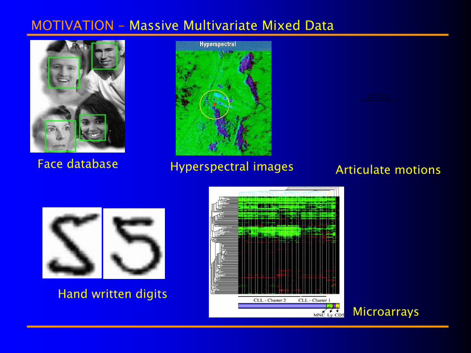
MOTIVATION – Massive Multivariate Mixed Data

Face database

Hand written digits

Hyperspectral images

Microarrays

Articulate motions

QuickTime™ and aBMP decompressor

are needed to see this picture.

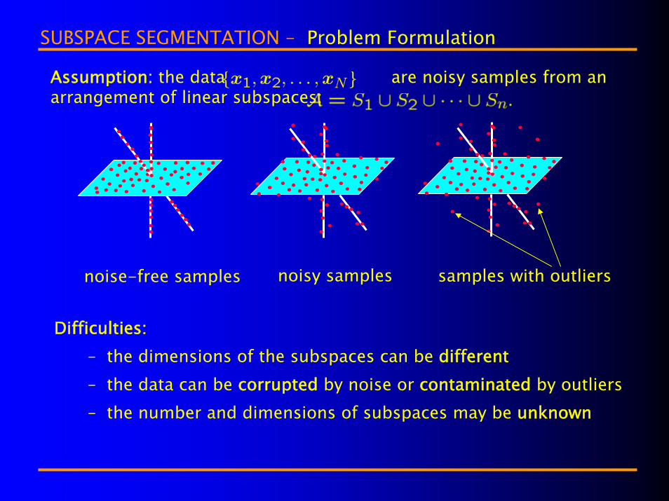
SUBSPACE SEGMENTATION – Problem Formulation

Difficulties:– the dimensions of the subspaces can be different– the data can be corrupted by noise or contaminated by outliers– the number and dimensions of subspaces may be unknown

Assumption: the data are noisy samples from an arrangement of linear subspaces:

noise-free samples noisy samples samples with outliers

SUBSPACE SEGMENTATION – Statistical Approaches

Assume that the data are i.i.d. samples from a mixture of probabilistic distributions:

Essentially iterate between data segmentation and model estimation.

Solutions:• Expectation Maximization (EM) for the maximum-likelihood estimate

[Dempster et. al.’77], e.g., Probabilistic PCA [Tipping-Bishop’99]:

• K-Means for a minimax-like estimate [Forgy’65, Jancey’66, MacQueen’67], e.g., K-Subspaces [Ho and Kriegman’03]:

SUBSPACE SEGMENTATION – An Algebro-Geometric Approach

Idea: a union of linear subspaces is an algebraic set -- the zero set of a set of (homogeneous) polynomials:

Complexity exponential in the dimension and number of subspaces.

Solution:• Identify the set of polynomials of degree n that vanish on

• Gradients of the vanishing polynomials are normals to the subspaces

Generalized Principal Component Analysis, [Vidal-Ma-Sastry, IEEE Transactions PAMI’0

SUBSPACE SEGMENTATION – An Information-Theoretic Approach

Problem: If the number/dimension of subspaces not given and data corrupted

by noise and outliers, how to determine the optimal subspaces that fit the data?Solutions: Model Selection Criteria?– Minimum message length (MML) [Wallace-Boulton’68]– Minimum description length (MDL) [Rissanen’78]– Bayesian information criterion (BIC)– Akaike information criterion (AIC) [Akaike’77]– Geometric AIC [Kanatani’03], Robust AIC [Torr’98]

Key idea (MDL):• a good balance between model complexity and data fidelity.• minimize the length of codes that describe the model and the data:

with a quantization error optimal for the model.

LOSSY DATA COMPRESSION

Questions:

– What is the “gain” or “loss” of segmenting or merging data?

– How does tolerance of error affect segmentation results?

Basic idea: whether the number of bits required to store “the whole is more than the sum of its parts”?

LOSSY DATA COMPRESSION – Problem Formulation

– A coding scheme maps a set of vectors to a sequence of bits, from which we can decode The coding length is denoted as:

– Given a set of real-valued mixed data the optimal segmentation

minimizes the overall coding length:

where

LOSSY DATA COMPRESSION – Coding Length for Multivariate Data

Theorem.Given with

is the number of bits needed to encode the data s.t. .

A nearly optimal bound for even a small number of vectors drawn from a subspace or a Gaussian source.

Segmentation of Multivariate Mixed Data, [Ma-Derksen-Hong-Wright, PAMI’

LOSSY DATA COMPRESSION – Two Coding Schemes

Goal: code s.t. a mean squared error

Linear subspace Gaussian source

LOSSY DATA COMPRESSION – Properties of the Coding Length

2. Asymptotic Property:

At high SNR, this is the optimal rate distortion for a Gaussian source.

1. Commutative Property:For high-dimensional data, computing the coding length only needsthe kernel matrix:

3. Invariant Property:Harmonic Analysis is useful for data compression only when the data arenon-Gaussian or nonlinear ……… so is segmentation!

LOSSY DATA COMPRESSION – Why Segment?

partitioning:

sifting:

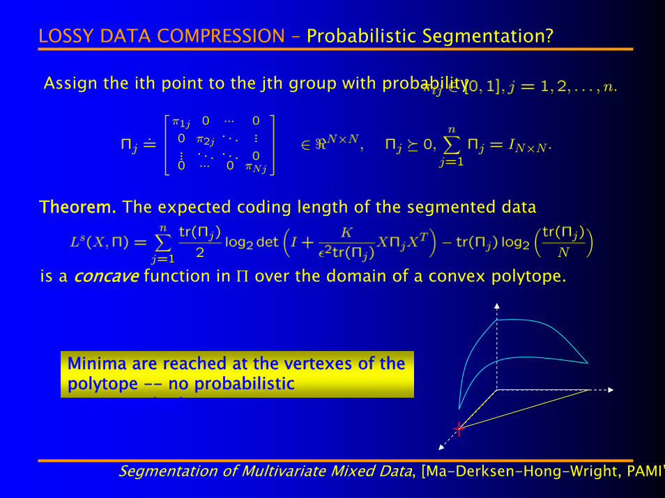
LOSSY DATA COMPRESSION – Probabilistic Segmentation?

is a concave function in Π over the domain of a convex polytope.

Minima are reached at the vertexes of the polytope -- no probabilistic segmentation!

Assign the ith point to the jth group with probability

Theorem. The expected coding length of the segmented data

Segmentation of Multivariate Mixed Data, [Ma-Derksen-Hong-Wright, PAMI’

LOSSY DATA COMPRESSION – Segmentation & Channel Capacity

A MIMO additive white Gaussian noise (AWGN) channel

has the capacity:

If allowing probabilistic grouping of transmitters, the expectedcapacity

is a concave function in Π over a convex polytope.Maximizing such a capacity is a convexproblem.

On Coding and Segmentation of Multivariate Mixed Data, [Ma-Derksen-Hong-Wright, PAMI

LOSSY DATA COMPRESSION – A Greedy (Agglomerative) Algorithm

Objective: minimizing the overall coding length

Input:

while true dochoose two sets such

that is minimal

ifthenelse breakendif

endOutput:

“Bottom-up” merge

QuickTime™ and aPNG decompressor

are needed to see this picture.

Segmentation of Multivariate Mixed Data via Lossy Coding and Compression, [Ma-Derksen-Hong-Wright, PAMI’07]

SIMULATIONS – Mixture of Almost Degenerate GaussiansNoisy samples from two lines and one plane in <3

Given Data Segmentation Results

ε0 = 0.01

Segmentation of Multivariate Mixed Data via Lossy Coding and Compression, [Ma-Derksen-Hong-Wright, PAMI’07]

ε0 = 0.08

SIMULATIONS – “Phase Transition”Rate v.s. distortion

0.08

ε0 = 0.08

#group v.s. distortion

Stability: the same segmentation for ε across 3 magnitudes!

0.08

steamwater

ice cubes

Segmentation of Multivariate Mixed Data via Lossy Coding and Compression, [Ma-Derksen-Hong-Wright, PAMI’07]

SIMULATIONS – Comparison with EM

100 x d uniformly distributed random samples from each subspace, corruptewith 4% noise. Classification rate averaged over 25 trials for each case.

Segmentation of Multivariate Mixed Data via Lossy Coding and Compression, [Ma-Derksen-Hong-Wright, PAMI’07]

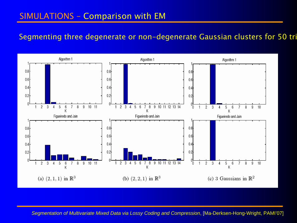
SIMULATIONS – Comparison with EM

Segmenting three degenerate or non-degenerate Gaussian clusters for 50 tria

Segmentation of Multivariate Mixed Data via Lossy Coding and Compression, [Ma-Derksen-Hong-Wright, PAMI’07]

SIMULATIONS – Robustness with Outliers

35.8% outliers 45.6%

71.5% 73.6%

Segmentation of Multivariate Mixed Data via Lossy Coding and Compression, [Ma-Derksen-Hong-Wright, PAMI’07]

SIMULATIONS – Affine Subspaces with Outliers

35.8% outliers 45.6%

66.2% 69.1%

Segmentation of Multivariate Mixed Data via Lossy Coding and Compression, [Ma-Derksen-Hong-Wright, PAMI’07]

SIMULATIONS – Piecewise-Linear Approximation of Manifolds

Swiss roll Mobius strip Torus Klein bottle

SIMULATIONS – Summary

– The minimum coding length objective automatically addresses the

model selection issue: the optimal solution is very stable and robust.

– The segmentation/merging is physically meaningful (measured in bits).

The results resemble phase transition in statistical physics.

– The greedy algorithm is scalable (polynomial in both K and N) and

converges well when ε is not too small w.r.t. the sample density.

Clustering from a Classification Perspective

Solution: Knowing the distributions and , the optimal classifier is the maximum a posteriori (MAP) classifier:

Difficulties: How to learn the two distributions from samples?(parametric, non-parametric, model selection, high-dimension, outliers…)

Goal: Construct a classifier such that the misclassification error

reaches minimum.

Assumption: The training data are drawn from a distribution

MINIMUM INCREMENTAL CODING LENGTH – Problem Formulation

Ideas: Using the lossy coding length

as a surrogate for the Shannon lossless coding length w.r.t. true distributions.

Classification Criterion: Minimum Incremental Coding Length (MICL)

Additional bits need to encode the test sample with the jth training set is

MICL (“Michael”) – Asymptotic Properties

Theorem: As the number of samples goes to infinity, the MICL criterion converges with probability one to the following criterion:

where?

is the “number of effective parameters” of the j-th model (class).

Theorem: The MICL classifier converges to the above asymptotic form at the rate of for some constant .

Minimum Incremental Coding Length (MICL), [Wright and Ma et. a.., NIPS’07]

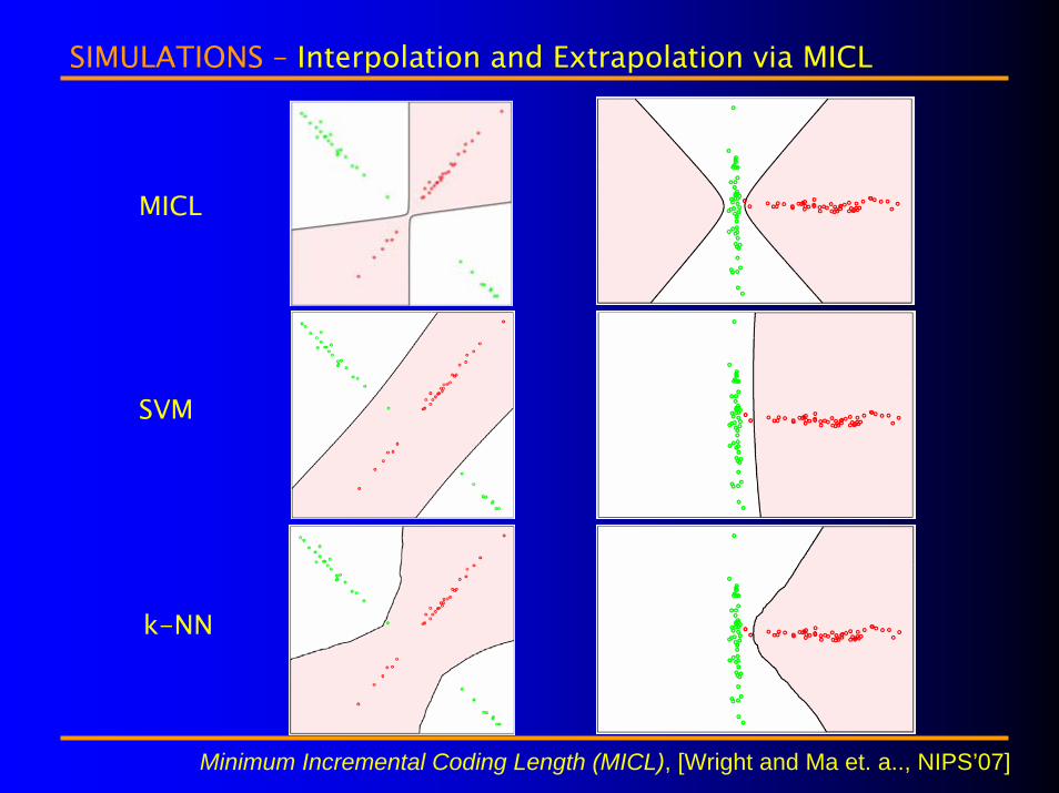
SIMULATIONS – Interpolation and Extrapolation via MICL

MICL

SVM

k-NN

Minimum Incremental Coding Length (MICL), [Wright and Ma et. a.., NIPS’07]

SIMULATIONS – Improvement over MAP and RDA [Friedman1989]

Two Gaussians in R2

isotropic (left)anisotropic

(right)(500 trials)

Three Gaussians in Rn

dim = ndim = n/2dim = 1

(500 trials)

Minimum Incremental Coding Length (MICL), [Wright and Ma et. a.., NIPS’07]

SIMULATIONS – Local and Kernel MICL

LMICL k-NN

KMICL-RBF SVM-RBF

Local MICL (LMICL): Applying MICL locally to the k-nearest neighbors of the test sample (frequencylist + Bayesianist).

Kernel MICL (KMICL): Incorporating MICL with a nonlinear kernel naturally through the identity (“kernelized” RDA):

Minimum Incremental Coding Length (MICL), [Wright and Ma et. a.., NIPS’07]

CONCLUSIONS

Assumptions: Data are in a high-dimensional space but have low-dimensional structures (subspaces or submanifolds).

Compression => Clustering & Classification:– Minimum (incremental) coding length subject to distortion.– Asymptotically optimal clustering and classification.– Greedy clustering algorithm (bottom-up, agglomerative).– MICL corroborates MAP, RDA, k-NN, and kernel methods.

Applications (Next Lectures):– Video segmentation, motion segmentation (Vidal)– Image representation & segmentation (Ma)– Others: microarray clustering, recognition of faces and

handwritten digits (Ma)

FUTURE DIRECTIONS

Theory– More complex structures: manifolds, systems, random

fields…– Regularization (ridge, lasso, banding etc.)– Sparse representation and subspace arrangements

Computation– Global optimality (random techniques, convex

optimization…)– Scalability: random sampling, approximation…

Future Application Domains– Image/video/audio classification, indexing, and retrieval– Hyper-spectral images and videos– Biomedical images, microarrays– Autonomous navigation, surveillance, and 3D mapping– Identification of hybrid linear/nonlinear systems

REFERENCES & ACKNOWLEGMENT

References:– Segmentation of Multivariate Mixed Data via Lossy Data

Compression, Yi Ma, Harm Derksen, Wei Hong, John Wright, PAMI, 2007.

– Classification via Minimum Incremental Coding Length (MICL), John Wright et. al., NIPS, 2007.

– Website: http://perception.csl.uiuc.edu/coding/home.htm

People:– John Wright, PhD Student, ECE Department, University of Illinois– Prof. Harm Derksen, Mathematics Department, University of

Michigan– Allen Yang (UC Berkeley) and Wei Hong (Texas Instruments R&D)– Zhoucheng Lin and Harry Shum, Microsoft Research Asia, China

Funding:– ONR YIP N00014-05-1-0633– NSF CAREER IIS-0347456, CCF-TF-0514955, CRS-EHS-0509151

““The whole is more than the sum of its The whole is more than the sum of its partsparts.”.”

----Aristotle Aristotle

Questions, please?

11/2003

Yi Ma, CVPR 2008