
LOSSLESS DATA COMPRESSION WITH POLAR CODES · LOSSLESS DATA COMPRESSION WITH POLAR CODES a thesis...
74
LOSSLESS DATA COMPRESSION WITH POLAR CODES a thesis submitted to the department of electrical and electronics engineering and the graduate school of engineering and science of bilkent university in partial fulfillment of the requirements for the degree of master of science By Semih C ¸ aycı August, 2013
-
Upload
vuongkhanh -
Category
Documents
-
view
245 -
download
0
Transcript of LOSSLESS DATA COMPRESSION WITH POLAR CODES · LOSSLESS DATA COMPRESSION WITH POLAR CODES a thesis...

LOSSLESS DATA COMPRESSION WITHPOLAR CODES
a thesis
submitted to the department of electrical and
electronics engineering
and the graduate school of engineering and science
of bilkent university
in partial fulfillment of the requirements
for the degree of
master of science
By
Semih Caycı
August, 2013

I certify that I have read this thesis and that in my opinion it is fully adequate,
in scope and in quality, as a thesis for the degree of Master of Science.
Prof. Dr. Orhan Arıkan and Prof. Dr. Erdal Arıkan(Advisors)
I certify that I have read this thesis and that in my opinion it is fully adequate,
in scope and in quality, as a thesis for the degree of Master of Science.
Assoc. Prof. Dr. Sinan Gezici
I certify that I have read this thesis and that in my opinion it is fully adequate,
in scope and in quality, as a thesis for the degree of Master of Science.
Assoc. Prof. Dr. Emre Aktas
Approved for the Graduate School of Engineering and Science:
Prof. Dr. Levent OnuralDirector of the Graduate School
ii
ABSTRACT
LOSSLESS DATA COMPRESSION WITH POLARCODES
Semih Caycı
M.S. in Electrical and Electronics Engineering
Supervisors: Prof. Dr. Orhan Arıkan and Prof. Dr. Erdal Arıkan
August, 2013
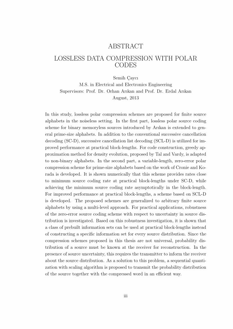
In this study, lossless polar compression schemes are proposed for finite source
alphabets in the noiseless setting. In the first part, lossless polar source coding
scheme for binary memoryless sources introduced by Arıkan is extended to gen-
eral prime-size alphabets. In addition to the conventional successive cancellation
decoding (SC-D), successive cancellation list decoding (SCL-D) is utilized for im-
proved performance at practical block-lengths. For code construction, greedy ap-
proximation method for density evolution, proposed by Tal and Vardy, is adapted
to non-binary alphabets. In the second part, a variable-length, zero-error polar
compression scheme for prime-size alphabets based on the work of Cronie and Ko-
rada is developed. It is shown numerically that this scheme provides rates close
to minimum source coding rate at practical block-lengths under SC-D, while
achieving the minimum source coding rate asymptotically in the block-length.
For improved performance at practical block-lengths, a scheme based on SCL-D
is developed. The proposed schemes are generalized to arbitrary finite source
alphabets by using a multi-level approach. For practical applications, robustness
of the zero-error source coding scheme with respect to uncertainty in source dis-
tribution is investigated. Based on this robustness investigation, it is shown that
a class of prebuilt information sets can be used at practical block-lengths instead
of constructing a specific information set for every source distribution. Since the
compression schemes proposed in this thesis are not universal, probability dis-
tribution of a source must be known at the receiver for reconstruction. In the
presence of source uncertainty, this requires the transmitter to inform the receiver
about the source distribution. As a solution to this problem, a sequential quanti-
zation with scaling algorithm is proposed to transmit the probability distribution
of the source together with the compressed word in an efficient way.
iii

iv
Keywords: Polar codes, source polarization, source coding, lossless data compres-
sion.

OZET
KUTUPSAL KODLARLA YITIMSIZ VERI SIKISTIRMA
Semih Caycı
Elektrik ve Elektronik Muhendisligi, Yuksek Lisans
Tez Yoneticileri: Prof. Dr. Orhan Arıkan ve Prof. Dr. Erdal Arıkan
Agustos, 2013
Bu calısmada, gurultusuz ortamda sonlu kaynak alfabeleri icin yitimsiz kutup-
sal veri sıkıstırma yontemleri onerilmektedir. Ilk kısımda, Arıkan tarafından
tanıtılan, ikilik kaynaklar icin yitimsiz kutupsal kodlama yontemi genel asal
boyutlu kaynak alfabelerine genisletilmistir. Konvansiyonel ardısık iptal kod
cozucusune ek olarak, pratik blok uzunluklarında iyilestirilmis performans icin
ardısık iptal liste kod cozucusu kullanılmıstır. Kod yapımı icin, Tal ve Vardy
tarafından onerilen yogunluk evrimi icin acgozlu yaklasıklama algoritması iki-
lik olmayan kaynak alfabelerine uyarlanmıstır. Ikinci bolumde Cronie ve Ko-
rada’nın calısmaları esas alınarak, asal boyutlu alfabeler icin degisken uzun-
luklu, sıfır hata kutupsal sıkıstırma seması gelistirilmistir. Onerilen kodlama
semasının ardısık iptal kod cozucusu ile blok uzunluguyla asimptotik olarak
minimum kaynak kodlama oranına erismenin yanı sıra pratik blok uzunluk-
larında minimum kaynak kodlama oranına yakın oranlar sagladıgı numerik
olarak gosterilmektedir. Pratik blok uzunluklarında iyilestirilmis performans
icin ardısık iptal liste kod cozucusu tabanlı bir sema gelistirilmistir. Onerilen
yontemler, coklu seviye yaklasımı kullanılarak rastgele sonlu kaynak alfabeler-
ine genellestirilmistir. Pratik uygulamalar icin, onerilen sıfır hata sıkıstırma
yonteminin kaynak dagılımındaki belirsizlige karsı gurbuzlugu arastırılmıstır. Bu
arastırma esas alınarak, pratik blok uzunluklarında her kaynak dagılımı icin ozel
bir enformasyon kumesi olusturmak yerine onceden insa edilmis enformasyon
kumeleri obegi kullanılabilecegi gosterilmistir. Bu tezde onerilen sıkıstırma
yontemleri evrensel olmadıgı icin bir kaynagın olasılık dagılımı alıcıda bilin-
melidir. Bu durum, kaynak belirsizligi varlıgında vericinin alıcıyı kaynak dagılımı
hakkında bilgilendirmesini zorunlu kılar. Bu soruna bir cozum olarak, kaynak
olasılık dagılımını etkin bir sekilde sıkıstırılmıs kelime ile gonderebilmek icin bir
olceklemeli sırasal basamaklama algoritması onerilmistir.
Anahtar sozcukler : Kutupsal kodlar, kaynak kutuplastırma, kaynak kodlama,
v

vi
yitimsiz veri sıkıstırma.

Acknowledgement
I would like to thank my supervisor Prof. Orhan Arıkan for his persistent help and
guidance in all stages of this thesis. This thesis could not have been completed
without his support. I would like to thank Prof. Erdal Arıkan for insightful
comments and suggestions, which have been key in this thesis. I consider myself
very fortunate to work on polar codes under their supervision.
This work was supported by The Scientific and Technological Research Coun-
cil of Turkey (TUBITAK) under contract no. 110E243. I am very grateful to
TUBITAK for funding my thesis.
I would like to dedicate this thesis to the memory of my grandmother.
vii
Contents
1 Introduction 1
1.1 Lossless Data Compression: Definitions and Theoretical Limits . . 1
1.2 Review of the Related Work . . . . . . . . . . . . . . . . . . . . . 2
1.3 Outline . . . . . . . . . . . . . . . . . . . . . . . . . . . . . . . . . 4
2 Lossless Data Compression with Polar Codes 6
2.1 Preliminaries . . . . . . . . . . . . . . . . . . . . . . . . . . . . . 6
2.2 Encoding . . . . . . . . . . . . . . . . . . . . . . . . . . . . . . . 9
2.3 Decoding . . . . . . . . . . . . . . . . . . . . . . . . . . . . . . . . 9
2.3.1 Successive Cancellation Decoder . . . . . . . . . . . . . . . 11
2.3.2 Successive Cancellation List Decoder . . . . . . . . . . . . 12
2.4 Code Construction . . . . . . . . . . . . . . . . . . . . . . . . . . 14
2.4.1 Density Evolution . . . . . . . . . . . . . . . . . . . . . . . 14
2.4.2 Greedy Approximation Algorithm for Code Construction . 19
2.5 Numerical Results . . . . . . . . . . . . . . . . . . . . . . . . . . . 24
viii
CONTENTS ix
3 Oracle-Based Lossless Polar Compression 28
3.1 Introduction . . . . . . . . . . . . . . . . . . . . . . . . . . . . . . 28
3.2 Preliminaries . . . . . . . . . . . . . . . . . . . . . . . . . . . . . 29
3.3 Encoding . . . . . . . . . . . . . . . . . . . . . . . . . . . . . . . 29
3.3.1 Encoding with Successive Cancellation Decoder . . . . . . 30
3.3.2 Encoding with Successive Cancellation List Decoder . . . . 32
3.4 Decoding . . . . . . . . . . . . . . . . . . . . . . . . . . . . . . . . 33
3.4.1 Successive Cancellation Decoder for Oracle-Based Com-
pression . . . . . . . . . . . . . . . . . . . . . . . . . . . . 33
3.4.2 Successive Cancellation List Decoder for Oracle-Based
Compression . . . . . . . . . . . . . . . . . . . . . . . . . . 34
3.5 Compression of Sources over Arbitrary Finite Alphabets . . . . . 35
3.6 Source Distribution Uncertainty at the Receiver . . . . . . . . . . 37
3.6.1 Sequential Quantization with Scaling Algorithm for Prob-
ability Mass Functions . . . . . . . . . . . . . . . . . . . . 38
3.6.2 Information Sets under Source Uncertainty and the Con-
cept of Class of Information Sets . . . . . . . . . . . . . . 40
3.7 Numerical Results . . . . . . . . . . . . . . . . . . . . . . . . . . . 49
4 Conclusions 57
List of Figures
1.1 Lossless source coding with side information. . . . . . . . . . . . . 2
2.1 Recursive polar transformation of XN−10 . . . . . . . . . . . . . . . 7
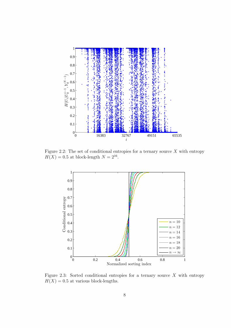
2.2 The set of conditional entropies for a ternary sourceX with entropy
H(X) = 0.5 at block-length N = 216. . . . . . . . . . . . . . . . . 8
2.3 Sorted conditional entropies for a ternary source X with entropy
H(X) = 0.5 at various block-lengths. . . . . . . . . . . . . . . . . 8
2.4 An example SCL-D tree for q = 3, L = 4 and N = 23. . . . . . . . 13
2.5 Basic polar transform. . . . . . . . . . . . . . . . . . . . . . . . . 16
2.6 Density evolution at block-length N . . . . . . . . . . . . . . . . . 18
2.7 Block error rates in the compression of a source with distribution
pX = (0.84, 0.09, 0.07) at block-length N = 210 under SCL-D
with L = 1, 2, 4, 8, 32. . . . . . . . . . . . . . . . . . . . . . . . . . 24
2.8 Symbol error rates in the compression of a source with distribution
pX = (0.84, 0.09, 0.07) at block-length N = 210 under SCL-D with
L = 1, 2, 4, 8, 32. . . . . . . . . . . . . . . . . . . . . . . . . . . . . 25
x
LIST OF FIGURES xi
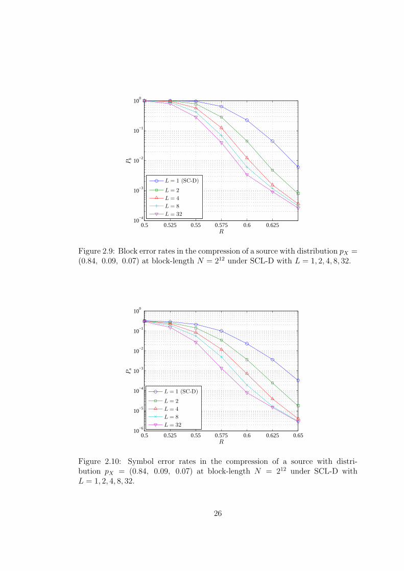
2.9 Block error rates in the compression of a source with distribution
pX = (0.84, 0.09, 0.07) at block-length N = 212 under SCL-D
with L = 1, 2, 4, 8, 32. . . . . . . . . . . . . . . . . . . . . . . . . . 26
2.10 Symbol error rates in the compression of a source with distribution
pX = (0.84, 0.09, 0.07) at block-length N = 212 under SCL-D with
L = 1, 2, 4, 8, 32. . . . . . . . . . . . . . . . . . . . . . . . . . . . . 26
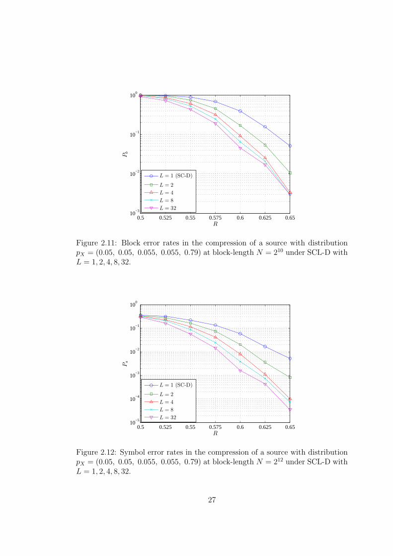
2.11 Block error rates in the compression of a source with distribution
pX = (0.05, 0.05, 0.055, 0.055, 0.79) at block-length N = 210
under SCL-D with L = 1, 2, 4, 8, 32. . . . . . . . . . . . . . . . . . 27
2.12 Symbol error rates in the compression of a source with distribution
pX = (0.05, 0.05, 0.055, 0.055, 0.79) at block-length N = 212
under SCL-D with L = 1, 2, 4, 8, 32. . . . . . . . . . . . . . . . . . 27
3.1 Oracle-based lossless polar compression scheme. . . . . . . . . . . 30
3.2 (0101)-configuration for the compression of (X, Y ). . . . . . . . . 35
3.3 The cost function JN(pX ,ϕq(pi)) with respect to H(ϕq(pi)) for
pX = (0.75, 0.21, 0.04), β = 6, and N = 210. . . . . . . . . . . . . 42
3.4 Probability distribution of pX ∼ Dir((3, 4, 5)). . . . . . . . . . . . 43
3.5 Construction of C with C = 32 over M(3). pi is spotted for all
i = 0, 1, . . . , C − 1, and entropy is shown as a density plot. . . . . 44
3.6 Independent and identically distributed realizations from pX ∼
Dir((1, 1, 1)) for cost analysis at block-length N = 210. . . . . . . 45
3.7 JN(pX ,ϕq(pi∗)) and H(pX) − H(ϕq(pi∗)) values at block-length
N = 210 for uniformly distributed pX . . . . . . . . . . . . . . . . . 45
3.8 Independent and identically distributed realizations from pX ∼
Dir((1, 1, 1)) for cost analysis at block-length N = 212. . . . . . . 47
LIST OF FIGURES xii
3.9 JN(pX ,ϕq(pi∗)) and H(pX) − H(ϕq(pi∗)) values at block-length
N = 212 for uniformly distributed pX . . . . . . . . . . . . . . . . . 47
3.10 Performance comparison of CIS construction techniques for ternary
sources of length N = 210. . . . . . . . . . . . . . . . . . . . . . . 48
3.11 Average compression rates for ternary sources under SC-D at
block-lengths N = 28, 29, . . . , 215. . . . . . . . . . . . . . . . . . . 49
3.12 The improvement in the expected code rate by SCL-D for a ternary
source with distribution p2 = (0.07, 0.09, 0.84) at various block-
lengths. . . . . . . . . . . . . . . . . . . . . . . . . . . . . . . . . 50
3.13 Expected code rates for a 6-ary source Z = (X, Y ) with probability
distribution pZ = (0.0077, 0.7476, 0.0675, 0.0623, 0.0924, 0.0225).
Base-2 entropy values are marked by dotted lines. . . . . . . . . . 51
3.14 The probability distribution of a source Z = (Z7, Z6, . . . , Z0)2 with
alphabet size q = 256. . . . . . . . . . . . . . . . . . . . . . . . . 52
3.15 E[Rk] and H(Zk|Zk−10 ) values for each k at block-length N = 214. 52
3.16 The average code rate E[R|pX ] values if pX is chosen randomly
such that H(pX) ∼ U [0.2, 0.7], C = 8, N = 212, and β = 3 . . . . 53
3.17 The average code rate E[R|pX ] values if pX is chosen randomly
such that H(pX) ∼ U [0.2, 0.7], C = 16, N = 212, and β = 3 . . . 54
3.18 The average code rate E[R|pX ] values if pX is chosen randomly
such that H(pX) ∼ U [0.2, 0.7], C = 8, N = 214, and β = 3 . . . . 55
3.19 The region D over which pX is distributed uniformly. . . . . . . . 56
3.20 The average code rate E[R|pX ] values for C = 8, N = 212, and β = 6 56
Chapter 1
Introduction
The subject of this thesis is the compression of discrete memoryless sources by us-
ing polar codes in the noiseless setting. In most practical compression problems,
such as discrete cosine transform-based image compression, zero-error compres-
sion of memoryless sources over a non-binary alphabet is required. The objective
in this problem is to develop compression schemes that provide rates close to
minimum source coding rate, the entropy of the source, by using low complex-
ity encoding and decoding algorithms. In this thesis, data compression schemes
based on polarization, introduced in [1], that have low complexity encoding and
decoding algorithms and an efficient deterministic code construction method are
proposed as a solution to the problem.
1.1 Lossless Data Compression: Definitions and
Theoretical Limits
In this thesis, lossless compression of discrete memoryless sources with side in-
formation in the noiseless setting is considered. Let (X, Y ) be a pair of random
variables over X ×Y with a joint probability mass function pX,Y . Throughout the
thesis, unless stated otherwise, X represents the source to be compressed, and
1
Y represents side information. The cardinality of the source alphabet, denoted
as |X |, is a positive integer q < ∞, and Y is a finite set. For a positive inte-
ger block-length N , N independent and identically distributed (iid) realizations
{(Xi, Yi), i = 0, 1, . . . , N − 1} from pX,Y are taken and vectors XN−10 and Y N−1
0
are obtained. Side information vector Y N−10 is assumed to be known at encoder
and decoder. This scenario is called (0101)-scheme in [2], and conditional source
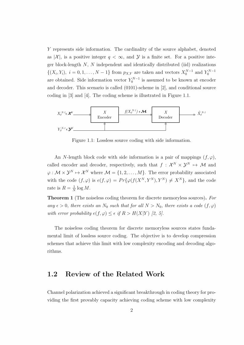
coding in [3] and [4]. The coding scheme is illustrated in Figure 1.1.
Figure 1.1: Lossless source coding with side information.
An N -length block code with side information is a pair of mappings (f, ϕ),
called encoder and decoder, respectively, such that f : XN × YN 7→ M and
ϕ : M×YN 7→ XN where M = {1, 2, . . . ,M}. The error probability associated
with the code (f, ϕ) is e(f, ϕ) = Pr{ϕ(f(XN , Y N), Y N) 6= XN}, and the code
rate is R = 1NlogM .
Theorem 1 (The noiseless coding theorem for discrete memoryless sources). For
any ǫ > 0, there exists an N0 such that for all N > N0, there exists a code (f, ϕ)
with error probability e(f, ϕ) ≤ ǫ if R > H(X|Y ) [2, 5].
The noiseless coding theorem for discrete memoryless sources states funda-
mental limit of lossless source coding. The objective is to develop compression
schemes that achieve this limit with low complexity encoding and decoding algo-
rithms.
1.2 Review of the Related Work
Channel polarization achieved a significant breakthrough in coding theory for pro-
viding the first provably capacity achieving coding scheme with low complexity
2
encoding and decoding algorithms [1]. The application of polarization in source
coding is first considered in [6] and [7], which exploit the duality between channel
coding and source coding in the solution of the problem. As a complementary
to channel polarization, source polarization was introduced in [8], and a lossless
source coding scheme based on source polarization, which asymptotically achieves
minimum source coding rate was described. In [9], a zero-error, fixed-to-variable
length source coding scheme is developed for binary memoryless sources without
considering side information, using a similar approach as in [10] for data com-
pression in the noiseless setting. It was shown in [9] that the proposed scheme
provides rates close to minimum source coding rate at practical block-lengths
besides achieving it asymptotically in the block-length under successive cancel-
lation decoder (SC-D). In practice, cardinality of the source alphabet can be
large; thus a generalization to non-binary alphabets is necessary. In addition,
side information, if available, must be exploited for reduced code rates. In this
paper, compression schemes for arbitrary finite source alphabets that exploit side
information are proposed based on the ideas derived from [9].
Polarization concept was extended to arbitrary discrete memoryless channels
in [11], and it is shown that a polarization transform similar to the binary case
leads to polarization for prime-size alphabets. For simplicity and efficiency, po-
larization scheme used in this paper is based on this work.
Successive cancellation decoder (SC-D), proposed in [1], is the first known
decoding algorithm for polar codes that achieves channel capacity asymptoti-
cally in the block-length with a complexity of O(N logN). In order to improve
performance of polar codes at practical block-lengths, Tal and Vardy proposed
successive cancellation list decoder (SCL-D), an adaptation of the list decoding
algorithm for Reed-Muller codes proposed in [12], and they numerically showed
that SCL-D approaches maximum-likelihood (ML) decoding performance. For
improved finite-length performance, SCL-D-based data compression schemes are
introduced in this thesis.
Monte Carlo method was used for polar code construction in [1] to estimate
Bhattacharyya parameters, which are used in the selection of good channels.
3
In [13], Mori and Tanaka showed that density evolution can be utilized as a
method of deterministic code construction. However, due to its high computa-
tional complexity, direct application of their method proved to be impractical for
large block-lengths. Tal and Vardy proposed quantization methods to overcome
this problem, and they described an efficient polar code construction method
for binary discrete memoryless channels in [14]. For efficient code construction,
a greedy density evolution method for non-binary alphabets, based on [14], is
presented in this thesis.
Robustness of polar source codes with respect to source uncertainty is an-
alyzed in [15]. It was shown that the information set constructed for a q-ary
probability distribution p0 is included in another information set that is con-
structed for a q-ary distribution p1 circularly dominated by p0. In this respect, it
was concluded that source coding at rate R = H(p1) ≥ H(p0) can be performed
asymptotically in the block-length. In this thesis, robustness of the proposed
scheme is analyzed from two perspectives including this, and efficient schemes for
practical applications in the presence of source uncertainty is proposed.
1.3 Outline
The outline of the thesis is as follows.
In Chapter 2, source polarization is briefly reviewed, and a fixed-to-fixed
length lossless source coding scheme for non-binary discrete memoryless sources
based on source polarization is described as a generalization of [8]. An efficient
greedy algorithm based on density evolution is proposed for polar code construc-
tion.
In Chapter 3, fixed-to-variable length, zero-error lossless polar compression
scheme introduced by Cronie and Korada is generalized to prime-size alphabets.
In order to reduce code rate at practical block-lengths, a compression scheme
based on SCL-D is proposed. These schemes for prime-size alphabets are gen-
eralized to arbitrary finite source alphabets by using a specific scenario for the
4

compression of correlation sources, and it is shown that minimum source coding
rate can be achieved by this scheme. Robustness of the proposed compression
scheme with respect to source uncertainty is investigated. Based on this investiga-
tion, in order to transmit the source distribution at the expense of extra overhead
in the presence of source uncertainty, a sequential quantization with scaling al-
gorithm is proposed. In order to reduce computational complexity in practical
applications, a method for constructing and using a pre-constructed information
sets is proposed.
Finally, conclusions and future work are presented in Chapter 4.
5
Chapter 2
Lossless Data Compression with
Polar Codes
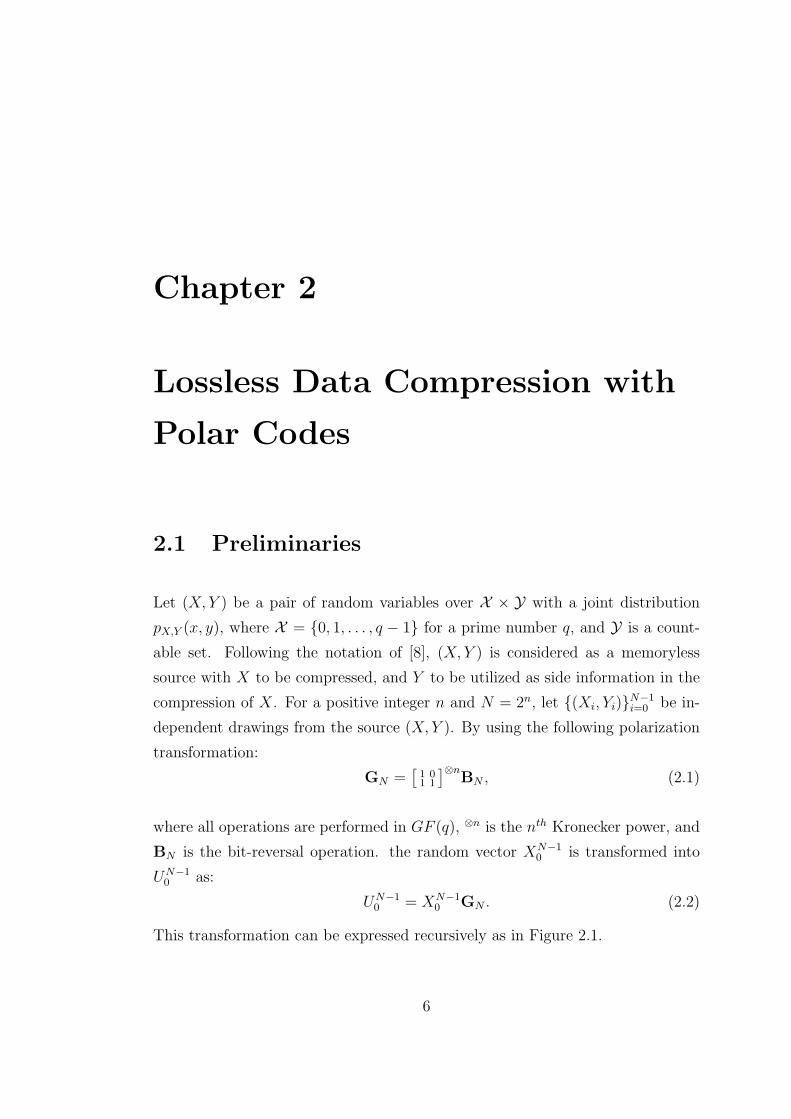
2.1 Preliminaries
Let (X, Y ) be a pair of random variables over X × Y with a joint distribution
pX,Y (x, y), where X = {0, 1, . . . , q − 1} for a prime number q, and Y is a count-
able set. Following the notation of [8], (X, Y ) is considered as a memoryless
source with X to be compressed, and Y to be utilized as side information in the
compression of X. For a positive integer n and N = 2n, let {(Xi, Yi)}N−1i=0 be in-
dependent drawings from the source (X, Y ). By using the following polarization
transformation:
GN =[1 01 1
]⊗nBN , (2.1)
where all operations are performed in GF (q), ⊗n is the nth Kronecker power, and
BN is the bit-reversal operation. the random vector XN−10 is transformed into
UN−10 as:
UN−10 = XN−1
0 GN . (2.2)
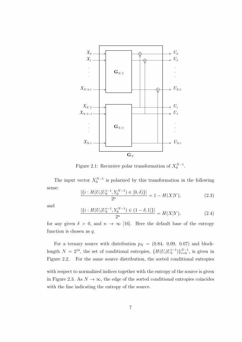
This transformation can be expressed recursively as in Figure 2.1.
6
X0X1
XN/2-1
XN/2XN/2+1
XN-1
U0U2
UN-2
U1U3
UN-1
GN/2
GN/2
GN
.
.
.
.
.
.
.
.
.
.
.
.
Figure 2.1: Recursive polar transformation of XN−10 .
The input vector XN−10 is polarized by this transformation in the following
sense:|{i : H(Ui|U
i−10 , Y N−1
0 ) ∈ [0, δ)}|
2n= 1−H(X|Y ), (2.3)
and|{i : H(Ui|U
i−10 , Y N−1
0 ) ∈ (1− δ, 1]}|
2n= H(X|Y ), (2.4)
for any given δ > 0, and n → ∞ [16]. Here the default base of the entropy
function is chosen as q.
For a ternary source with distribution pX = (0.84, 0.09, 0.07) and block-
length N = 214, the set of conditional entropies, {H(Ui|Ui−10 )}N−1
i=0 , is given in
Figure 2.2. For the same source distribution, the sorted conditional entropies
with respect to normalized indices together with the entropy of the source is given
in Figure 2.3. As N → ∞, the edge of the sorted conditional entropies coincides
with the line indicating the entropy of the source.
7
0 16383 32767 49151 655350
0.1
0.2
0.3
0.4
0.5
0.6
0.7
0.8
0.9
1
H(U
i|U
i−
1
0,Y
N−
1
0)
i
Figure 2.2: The set of conditional entropies for a ternary source X with entropyH(X) = 0.5 at block-length N = 216.
0 0.2 0.4 0.6 0.8 10
0.1
0.2
0.3
0.4
0.5
0.6
0.7
0.8
0.9
1
Normalized sorting index
Conditio
nalen
tropy
n = 10
n = 12
n = 14
n = 16
n = 18
n = 20n → ∞
Figure 2.3: Sorted conditional entropies for a ternary source X with entropyH(X) = 0.5 at various block-lengths.
8

2.2 Encoding
Based on source polarization, a lossless source coding scheme for binary memory-
less sources is introduced in [8]. The basic idea is to transmit symbols which can
be reconstructed using previous symbols, i.e., those with high H(Ui|Ui−10 , Y N−1
0 ).
Let R ∈ (0, 1) be a given rate, and r = ⌈NR⌉. The set of indices corresponding
to the r highest H(Ui|Ui−10 , Y N−1
0 ) terms is defined as the information set:
IX|Y (N,R) = {i ∈ {0, 1, . . . , N − 1} : H(Ui|Ui−10 , Y N−1
0 ) ≥ δ(r)} (2.5)
where δ(r) corresponds to the rth highest H(Ui|Ui−10 , Y N−1
0 ). The information
set is assumed to be known at both encoder and decoder, and shown as IX|Y in
the short form.
In the encoding process, a source realization xN−10 is transformed into uN−1
0 by
the polar transformation given in (2.2). Then, the vector consisting of elements of
uN−10 corresponding to the information set IX|Y , denoted as uIX|Y
, is transmitted
as the codeword. The complexity of encoding is O(N logN) [1].
2.3 Decoding
In this section, two decoding schemes, namely successive cancellation decoder
(SC-D) and successive cancellation list decoder (SCL-D), will be described. In
both schemes, recursive computation of path probabilities, i.e., Pr{U i−10 =
ui−10 |Y N−1
0 = yN−10 } for all i ∈ Ic
X|Y = {0, 1, . . . , N − 1}\IX|Y , plays a funda-
mental role. Thus, the recursive computation scheme will be derived first.
The probability of observing a sequence uN−10 at the output of the polarization
transform is defined as follows:
PN(uN−10 |yN−1
0 ) , Pr{UN−10 = uN−1
0 |Y N−10 = yN−1
0 }. (2.6)
Lemma 1. The probability of a sequence uN−10 at the output of the polarization
9
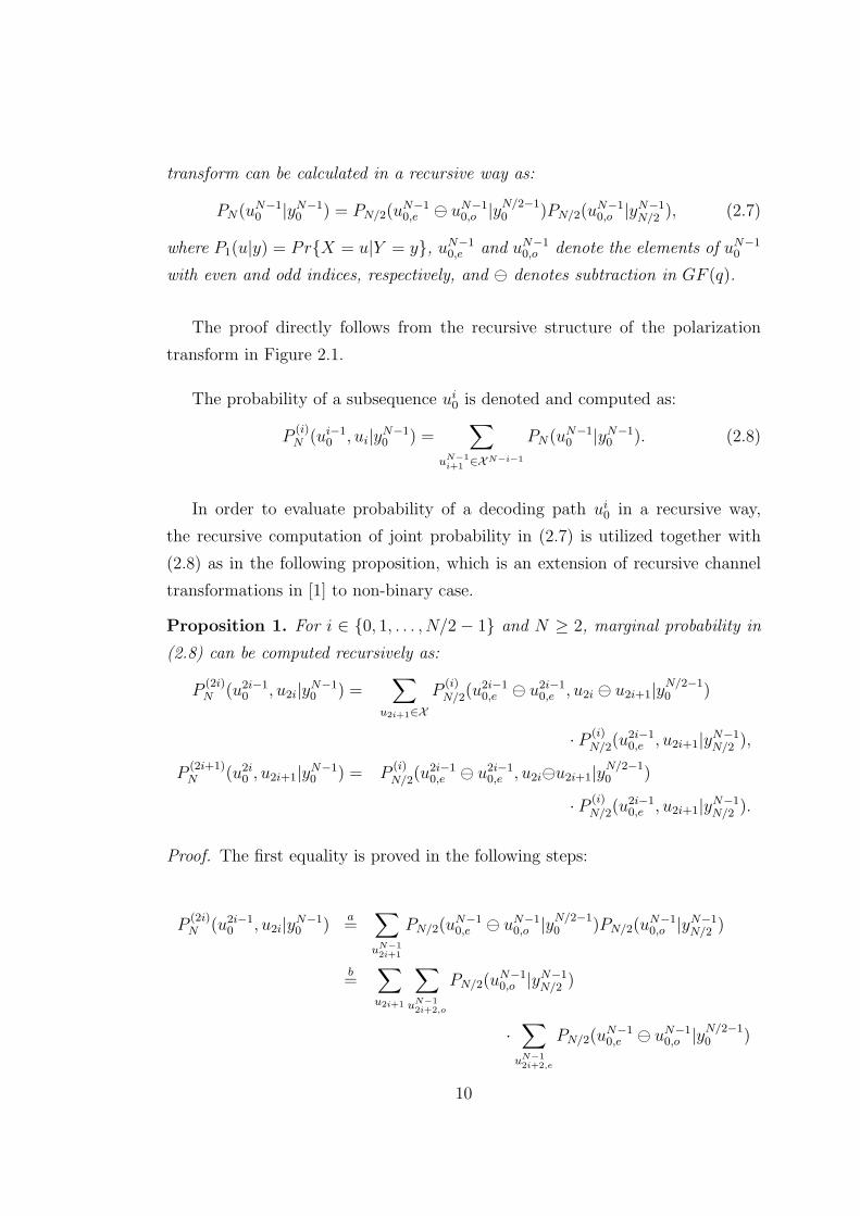
transform can be calculated in a recursive way as:
PN(uN−10 |yN−1
0 ) = PN/2(uN−10,e ⊖ uN−1
0,o |yN/2−10 )PN/2(u
N−10,o |yN−1
N/2 ), (2.7)
where P1(u|y) = Pr{X = u|Y = y}, uN−10,e and uN−1
0,o denote the elements of uN−10
with even and odd indices, respectively, and ⊖ denotes subtraction in GF (q).
The proof directly follows from the recursive structure of the polarization
transform in Figure 2.1.
The probability of a subsequence ui0 is denoted and computed as:
P(i)N (ui−1
0 , ui|yN−10 ) =
∑
uN−1
i+1∈XN−i−1
PN(uN−10 |yN−1
0 ). (2.8)
In order to evaluate probability of a decoding path ui0 in a recursive way,
the recursive computation of joint probability in (2.7) is utilized together with
(2.8) as in the following proposition, which is an extension of recursive channel
transformations in [1] to non-binary case.
Proposition 1. For i ∈ {0, 1, . . . , N/2 − 1} and N ≥ 2, marginal probability in
(2.8) can be computed recursively as:
P(2i)N (u2i−1
0 , u2i|yN−10 ) =
∑
u2i+1∈X
P(i)N/2(u
2i−10,e ⊖ u2i−1
0,e , u2i ⊖ u2i+1|yN/2−10 )
· P(i)N/2(u
2i−10,e , u2i+1|y
N−1N/2 ),
P(2i+1)N (u2i
0 , u2i+1|yN−10 ) = P
(i)N/2(u
2i−10,e ⊖ u2i−1
0,e , u2i⊖u2i+1|yN/2−10 )
· P(i)N/2(u
2i−10,e , u2i+1|y
N−1N/2 ).
Proof. The first equality is proved in the following steps:
P(2i)N (u2i−1
0 , u2i|yN−10 )
a=
∑
uN−1
2i+1
PN/2(uN−10,e ⊖ uN−1
0,o |yN/2−10 )PN/2(u
N−10,o |yN−1
N/2 )
b=
∑
u2i+1
∑
uN−1
2i+2,o
PN/2(uN−10,o |yN−1
N/2 )
·∑
uN−1
2i+2,e
PN/2(uN−10,e ⊖ uN−1
0,o |yN/2−10 )
10
c=
∑
u2i+1
∑
uN−1
2i+2,o
P(i)N/2(u
2i−10,e ⊖ u2i−1
0,o , u2i ⊖ u2i+1|yN/2−10 )
· PN/2(uN−10,o |yN−1
N/2 )
d=
∑
u2i+1
P(i)N/2(u
2i−10,e ⊖u2i−1
0,o , u2i ⊖ u2i+1|yN/2−10 )
· P(i)N/2(u
2i−10,e , u2i+1|y
N−1N/2 ).
(a) directly follows from Lemma 2.7. From (b) to (c), we devise the fact that
marginalizing inner probability with first input argument uN−10,o ⊖uN−1
0,e over uN−12i+2,e
for a fixed uN−12i+2,o corresponds to marginalization over uN−1
2i+2,e ⊖ uN−12i+2,o. In (d), it
is considered that the marginalization over uN−12i+2,o does not affect the term with
first input argument u2i−10,e ⊖ u2i−1
0,o .
The second part of the proof is identical with the first part and omitted.
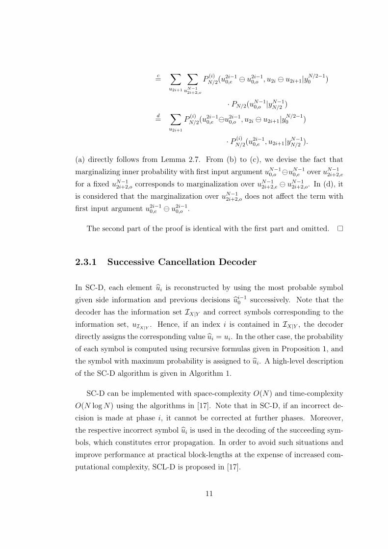
2.3.1 Successive Cancellation Decoder
In SC-D, each element ui is reconstructed by using the most probable symbol
given side information and previous decisions ui−10 successively. Note that the
decoder has the information set IX|Y and correct symbols corresponding to the
information set, uIX|Y. Hence, if an index i is contained in IX|Y , the decoder
directly assigns the corresponding value ui = ui. In the other case, the probability
of each symbol is computed using recursive formulas given in Proposition 1, and
the symbol with maximum probability is assigned to ui. A high-level description
of the SC-D algorithm is given in Algorithm 1.
SC-D can be implemented with space-complexity O(N) and time-complexity
O(N logN) using the algorithms in [17]. Note that in SC-D, if an incorrect de-
cision is made at phase i, it cannot be corrected at further phases. Moreover,
the respective incorrect symbol ui is used in the decoding of the succeeding sym-
bols, which constitutes error propagation. In order to avoid such situations and
improve performance at practical block-lengths at the expense of increased com-
putational complexity, SCL-D is proposed in [17].
11
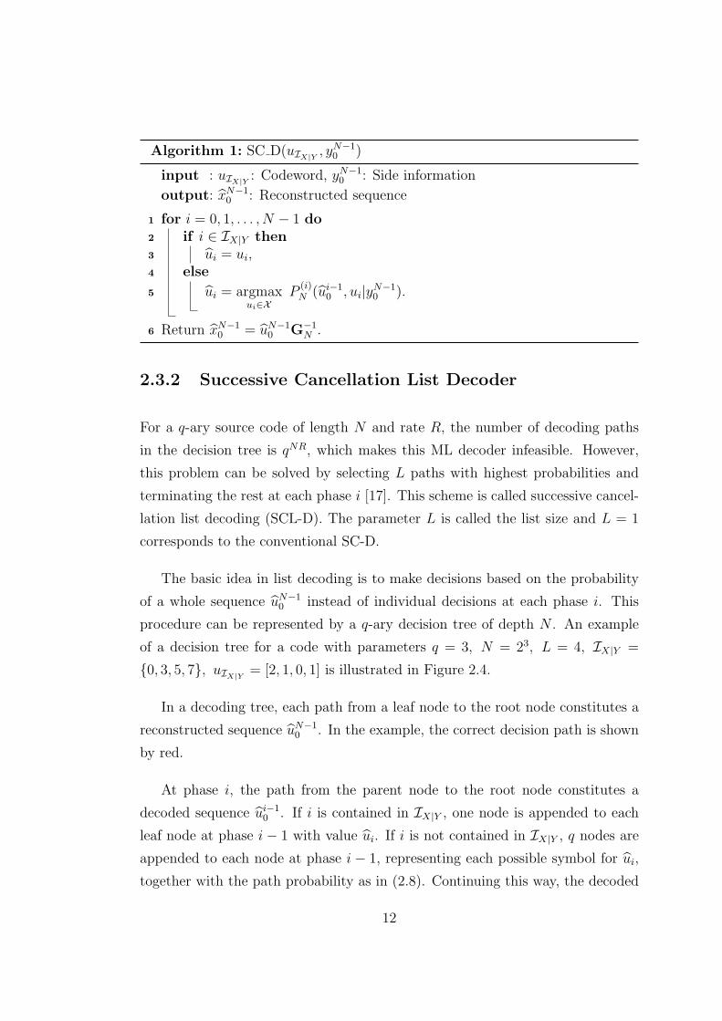
Algorithm 1: SC D(uIX|Y, yN−1
0 )
input : uIX|Y: Codeword, yN−1
0 : Side information
output: xN−10 : Reconstructed sequence
1 for i = 0, 1, . . . , N − 1 do
2 if i ∈ IX|Y then
3 ui = ui,4 else
5 ui = argmaxui∈X
P(i)N (ui−1
0 , ui|yN−10 ).
6 Return xN−10 = uN−1
0 G−1N .
2.3.2 Successive Cancellation List Decoder
For a q-ary source code of length N and rate R, the number of decoding paths
in the decision tree is qNR, which makes this ML decoder infeasible. However,
this problem can be solved by selecting L paths with highest probabilities and
terminating the rest at each phase i [17]. This scheme is called successive cancel-
lation list decoding (SCL-D). The parameter L is called the list size and L = 1
corresponds to the conventional SC-D.
The basic idea in list decoding is to make decisions based on the probability
of a whole sequence uN−10 instead of individual decisions at each phase i. This
procedure can be represented by a q-ary decision tree of depth N . An example
of a decision tree for a code with parameters q = 3, N = 23, L = 4, IX|Y =
{0, 3, 5, 7}, uIX|Y= [2, 1, 0, 1] is illustrated in Figure 2.4.
In a decoding tree, each path from a leaf node to the root node constitutes a
reconstructed sequence uN−10 . In the example, the correct decision path is shown
by red.
At phase i, the path from the parent node to the root node constitutes a
decoded sequence ui−10 . If i is contained in IX|Y , one node is appended to each
leaf node at phase i− 1 with value ui. If i is not contained in IX|Y , q nodes are
appended to each node at phase i − 1, representing each possible symbol for ui,
together with the path probability as in (2.8). Continuing this way, the decoded
12
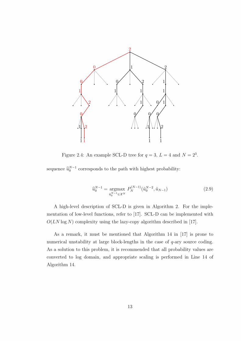
Figure 2.4: An example SCL-D tree for q = 3, L = 4 and N = 23.
sequence uN−10 corresponds to the path with highest probability:
uN−10 = argmax
uN−1
0∈XN
P(N−1)N (uN−2
0 , uN−1) (2.9)
A high-level description of SCL-D is given in Algorithm 2. For the imple-
mentation of low-level functions, refer to [17]. SCL-D can be implemented with
O(LN logN) complexity using the lazy-copy algorithm described in [17].
As a remark, it must be mentioned that Algorithm 14 in [17] is prone to
numerical unstability at large block-lengths in the case of q-ary source coding.
As a solution to this problem, it is recommended that all probability values are
converted to log domain, and appropriate scaling is performed in Line 14 of
Algorithm 14.
13
Algorithm 2: SCL D(uIX|Y, yN−1
0 , L)
input : uIX|Y: Codeword, yN−1
0 : Side information, L: List size
output: xN−10 : Reconstructed sequence
1 // Li: The set of active paths at phase i.
2 for i = 0, 1, . . . , N − 1 do
3 if i ∈ IX|Y then
4 Append ui to each ui−10 [l] ∈ Li−1, and obtain (ui−1
0 [l], ui)5 else
6 Append all ui ∈ X to each ui−10 [l] ∈ Li−1;
7 Calculate P(i)N (ui−1
0 [l], ui|yN−10 ) for all (ui−1
0 [l], ui) ∈ Li;8 Prune all but L paths with highest probabilities.
9 Return xN−10 = ( argmax
uN−1
0∈LN−1
P(N−1)N (uN−1
0 |yN−10 ))G−1
N .
2.4 Code Construction
In polar coding, it is assumed that the information set, IX|Y , is known at both
encoder and decoder. In order to construct IX|Y as in (2.5), the set of condi-
tional entropies {H(Ui|Ui−10 , Y N−1
0 )}N−1i=0 must be available. Except a small class
of examples, e.g., binary erasure channels in channel coding, analytic solutions
do not exist for computing conditional entropy values. As a solution, density evo-
lution is proposed for computing {H(Ui|Ui−10 , Y N−1
0 )}N−1i=0 , and constructing IX|Y
for any generic distribution pX,Y (x, y) [13, 14]. In this section, a greedy approxi-
mation algorithm for computing {H(Ui|Ui−10 , Y N−1
0 )}N−1i=0 using density evolution
is proposed for prime-size alphabets.
2.4.1 Density Evolution
Let p = (p0, p1, . . . , pq−1) ∈ Rq be a q-dimensional probability vector, i.e., pi >
0, ∀i andq−1∑i=0
pi = 1. q-ary entropy function is defined as follows:
H(p) =
q−1∑
i=0
pi log1
pi(2.10)
14
For f : X 7→ R, a function defined on X = {0, 1, . . . q−1}, [f(x)]q−1x=0 represents
q-dimensional vector formed by the values of f :
[f(x)]q−1x=0 = [f(0), f(1), . . . , f(q − 1)]
Let (X, Y ) be a pair of random variables over X × Y , X = {0, 1, . . . , q − 1},
with joint distribution pX,Y (x, y). The conditional entropy H(X|Y ) is computed
as follows:
H(X|Y ) =∑
y∈Y
pY (y)∑
x∈X
pX|Y (x|y) log1
pX|Y (x|y)(2.11)
=∑
y∈Y
pY (y)H([pX|Y (x|y)]q−1x=0)
Hence, for the computation of H(X|Y ), the set of (q + 1)-dimensional vectors
{(pY (y), [pX|Y (x|y)]q−1x=0)}y∈Y is needed. In density evolution, the objective is to
obtain {(pU i−1
0,Y N−1
0
(ui−10 , yN−1
0 ), [pUi|Ui−1
0,Y N−1
0
(u|ui−10 , yN−1
0 )]q−1u=0)}ui−1
0∈X i,yN−1
0∈YN
by evolving the distributions of the source through the polar transform so that
H(Ui|Ui−10 , Y N−1
0 ) can be computed.
Probability distributions of the pair of random variables (X, Y ) are expressed
in a list as follows:
X|Y ∼∑
y∈Y
pY (y)Q([pX|Y (x|y)]q−1x=0) (2.12)
Remark: Consider a random variable Z that is independent from X and
Y . Then, by notation, X|Y = X|Y, Z since for a fixed y, [pX|Y,Z(x|y, z)]q−1x=0 =
[pX|Y (x|y)]q−1x=0 for all z ∈ Z, and pY,Z(y, z) = pY (y)pZ(z) for all y, z, which
together imply that Z has no effect in the computation of conditional entropy.
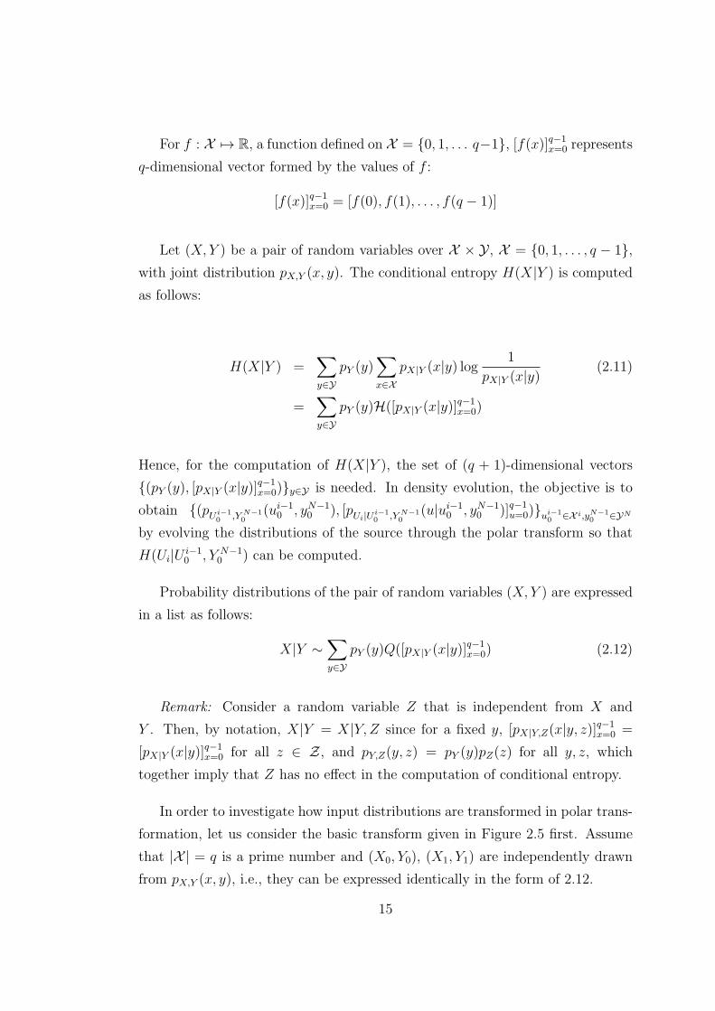
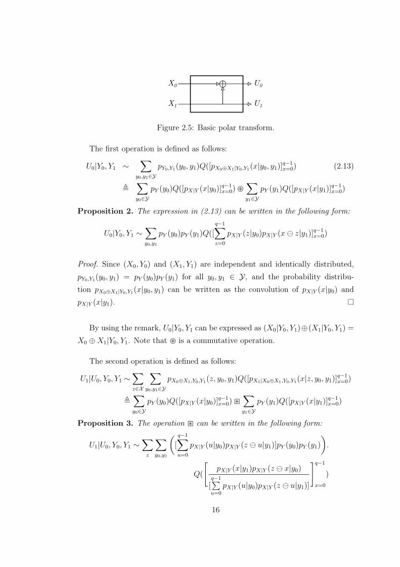
In order to investigate how input distributions are transformed in polar trans-
formation, let us consider the basic transform given in Figure 2.5 first. Assume
that |X | = q is a prime number and (X0, Y0), (X1, Y1) are independently drawn
from pX,Y (x, y), i.e., they can be expressed identically in the form of 2.12.
15
X0
X1
U0
U1
Figure 2.5: Basic polar transform.
The first operation is defined as follows:
U0|Y0, Y1 ∼∑
y0,y1∈Y
pY0,Y1(y0, y1)Q([pX0⊕X1|Y0,Y1
(x|y0, y1)]q−1x=0) (2.13)
,∑
y0∈Y
pY (y0)Q([pX|Y (x|y0)]q−1x=0) �
∑
y1∈Y
pY (y1)Q([pX|Y (x|y1)]q−1x=0)
Proposition 2. The expression in (2.13) can be written in the following form:
U0|Y0, Y1 ∼∑
y0,y1
pY (y0)pY (y1)Q([
q−1∑
z=0
pX|Y (z|y0)pX|Y (x⊖ z|y1)]q−1x=0)
Proof. Since (X0, Y0) and (X1, Y1) are independent and identically distributed,
pY0,Y1(y0, y1) = pY (y0)pY (y1) for all y0, y1 ∈ Y , and the probability distribu-
tion pX0⊕X1|Y0,Y1(x|y0, y1) can be written as the convolution of pX|Y (x|y0) and
pX|Y (x|y1).
By using the remark, U0|Y0, Y1 can be expressed as (X0|Y0, Y1)⊕(X1|Y0, Y1) =
X0 ⊕X1|Y0, Y1. Note that � is a commutative operation.
The second operation is defined as follows:
U1|U0, Y0, Y1 ∼∑
z∈X
∑
y0,y1∈Y
pX0⊕X1,Y0,Y1(z, y0, y1)Q([pX1|X0⊕X1,Y0,Y1
(x|z, y0, y1)]q−1x=0)
,∑
y0∈Y
pY (y0)Q([pX|Y (x|y0)]q−1x=0) �
∑
y1∈Y
pY (y1)Q([pX|Y (x|y1)]q−1x=0)
Proposition 3. The operation � can be written in the following form:
U1|U0, Y0, Y1 ∼∑
z
∑
y0,y1
([
q−1∑
u=0
pX|Y (u|y0)pX|Y (z ⊖ u|y1)]pY (y0)pY (y1)
).
Q(
[pX|Y (x|y1)pX|Y (z ⊖ x|y0)
[q−1∑u=0
pX|Y (u|y0)pX|Y (z ⊖ u|y1)]
]q−1
x=0
)
16
The proof is similar to Proposition 2.
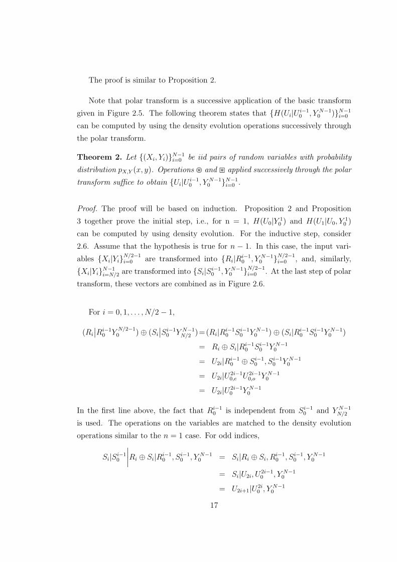
Note that polar transform is a successive application of the basic transform
given in Figure 2.5. The following theorem states that {H(Ui|Ui−10 , Y N−1
0 )}N−1i=0
can be computed by using the density evolution operations successively through
the polar transform.
Theorem 2. Let {(Xi, Yi)}N−1i=0 be iid pairs of random variables with probability
distribution pX,Y (x, y). Operations � and � applied successively through the polar
transform suffice to obtain {Ui|Ui−10 , Y N−1
0 }N−1i=0 .
Proof. The proof will be based on induction. Proposition 2 and Proposition
3 together prove the initial step, i.e., for n = 1, H(U0|Y10 ) and H(U1|U0, Y
10 )
can be computed by using density evolution. For the inductive step, consider
2.6. Assume that the hypothesis is true for n − 1. In this case, the input vari-
ables {Xi|Yi}N/2−1i=0 are transformed into {Ri|R
i−10 , Y N−1
0 }N/2−1i=0 , and, similarly,
{Xi|Yi}N−1i=N/2 are transformed into {Si|S
i−10 , Y N−1
0 }N/2−1i=0 . At the last step of polar
transform, these vectors are combined as in Figure 2.6.
For i = 0, 1, . . . , N/2− 1,
(Ri
∣∣Ri−10 Y
N/2−10 )⊕ (Si
∣∣Si−10 Y N−1
N/2 )=(Ri|Ri−10 Si−1
0 Y N−10 )⊕ (Si|R
i−10 Si−1
0 Y N−10 )
= Ri ⊕ Si|Ri−10 Si−1
0 Y N−10
= U2i|Ri−10 ⊕ Si−1
0 , Si−10 Y N−1
0
= U2i|U2i−10,e U2i−1
0,o Y N−10
= U2i|U2i−10 Y N−1
0
In the first line above, the fact that Ri−10 is independent from Si−1
0 and Y N−1N/2
is used. The operations on the variables are matched to the density evolution
operations similar to the n = 1 case. For odd indices,
Si|Si−10
∣∣∣∣Ri ⊕ Si|Ri−10 , Si−1
0 , Y N−10 = Si|Ri ⊕ Si, R
i−10 , Si−1
0 , Y N−10
= Si|U2i, U2i−10 , Y N−1
0
= U2i+1|U2i0 , Y N−1
0
17
U0|Y0N-1
GN/2
GN/2
GN
.
.
.
.
.
.
.
.
.
.
.
.
X0|Y0
X1|Y1
XN/2-1|YN/2-1
XN/2|YN/2
XN/2+1|YN/2+1
XN-1|YN-1
R0|Y0N/2-1
R1|R0,Y0N/2-1
RN/2-1|R0N/2-2,Y0
N/2-1
S0|YN/2N-1
S1|S0,YN/2N-1
SN/2-1|S0N/2-2,YN/2
N-1
U2|U01,Y0
N-1
UN-2|U0N-3,Y0
N-1
U1|U0,Y0N-1
U3|U02,Y0
N-1
UN-1|U0N-2,Y0
N-1
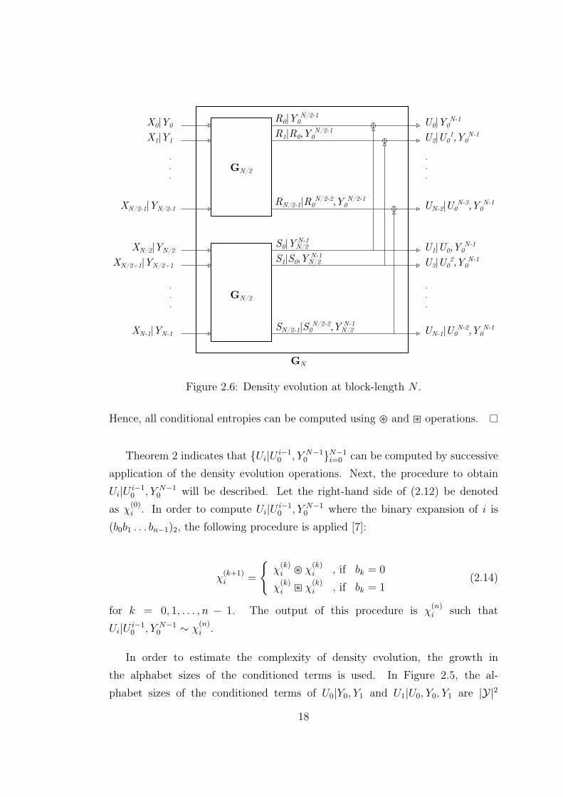
Figure 2.6: Density evolution at block-length N .
Hence, all conditional entropies can be computed using � and � operations.
Theorem 2 indicates that {Ui|Ui−10 , Y N−1
0 }N−1i=0 can be computed by successive
application of the density evolution operations. Next, the procedure to obtain
Ui|Ui−10 , Y N−1
0 will be described. Let the right-hand side of (2.12) be denoted
as χ(0)i . In order to compute Ui|U
i−10 , Y N−1
0 where the binary expansion of i is
(b0b1 . . . bn−1)2, the following procedure is applied [7]:
χ(k+1)i =
{χ(k)i � χ
(k)i , if bk = 0
χ(k)i � χ
(k)i , if bk = 1
(2.14)
for k = 0, 1, . . . , n − 1. The output of this procedure is χ(n)i such that
Ui|Ui−10 , Y N−1
0 ∼ χ(n)i .
In order to estimate the complexity of density evolution, the growth in
the alphabet sizes of the conditioned terms is used. In Figure 2.5, the al-
phabet sizes of the conditioned terms of U0|Y0, Y1 and U1|U0, Y0, Y1 are |Y|2
18
and |Y|2q, respectively. Note that if two different y, say y1 and y2, in the
RHS of (2.12) have the same [pX|Y (x|y)]q−1x=0, then they can be unified as
[pY (y1) + pY (y2)]Q([pX|Y (x|y1)]q−1x=0), which implies that the alphabet sizes are
upper bounds. At block-length N , the alphabet size becomes O(qN−1). Thus,
the direct application of density evolution in polar code construction infeasible.
Approximation methods are proposed to solve this problem [14]. In the following
subsection, approximation methods for q-ary code construction based on [14] will
be proposed.
2.4.2 Greedy Approximation Algorithm for Code Con-
struction
The basic idea in the approximation algorithm is to unify symbols y, y ∈ Y ,
whose unification changes the entropy of X|Y minimally, successively until the
alphabet size becomes lower than a given parameter µ. By such an approximation,
the growth in the number of (pY (y), [pX|Y (x|y)]q−1x=0) through the polar transform
can be controlled, hence efficient code construction can be performed.
Assume that we have X|Y ∼∑y∈Y
pY (y)Q([pX|Y (x|y)]q−1x=0) where |Y| > µ for a
given positive integer µ. Denote the conditional probability of X given a realiza-
tion y by pX|y, i.e., pX|y = [pX|Y (x|y)]q−1x=0. For y, y ∈ Y , the following operation
is performed to reduce the alphabet size of the side information:
pY (y)Q(pX|y) + pY (y)Q(pX|y) 7→ (pY (y) + pY (y))Q(p) (2.15)
for a valid probability vector p. The new alphabet, Y = Y\{y, y} ∪ {y}, has
cardinality |Y| − 1. In greedy approximation algorithm, symbol pairs y, y and
unified distribution p are chosen in an intelligent way at each step, and the
alphabet size is reduced by one. By successively applying the operation in (2.15),
the alphabet size is reduced below the given parameter, i.e., |Y| < µ.
A different approximation algorithm is proposed for non-binary polar code
construction in [18]. The main difference is that [18] involves parametrized quan-
tization levels, whereas the method presented here is based on a greedy algorithm
19
as in [14] and [19]. The algorithm that will be proposed here can be considered
as a modification of the mass merging algorithm in [19]. For detailed description
and analysis of mass merging and mass transportation algorithms, we refer to
[19].
Let X|Y ∼ χ be a source as defined in (2.12) with χ =∑y∈Y
pY (y)Q(pX|Y (x|y)),
y, y ∈ Y be given symbols for merging, and γ ∈ [0, 1]. Merging of these masses
with weight γ is the following transformation:
pY (y)Q(pX|y) + pY (y)Q(pX|y) 7→ (pY (y) + pY (y))Q(γpX|y + (1− γ)pX|y) (2.16)
This transformation corresponds to mass transportation if γ = 0 and γ = 1, and
degrading approximation (and mass merging as defined in [19]) if γ = pY (y)pY (y)+pY (y)
.
In order to define the approximation error due to (2.16), consider the following
function:
fy,y(γ) = (pY (y) + pY (y))H(γpX|y+(1− γ)pX|y) (2.17)
− pY (y)H(pX|y)− pY (y)H(pX|y).
The approximation error is defined as the change in the conditional entropy due
to the mass merging transformation:
ǫy,y(γ) = |fy,y(γ)|. (2.18)
For any y, y ∈ Y , the following proposition holds:
Proposition 4. fy,y(γ) = 0 has exactly one root in the interval (0, 1].
Proof. The case H(pX|y) = H(pX|y) is trivial: γ = 1 satisfy the claim. In order
to prove that the proposition holds for the non-trivial case, first, it is proved that
fy,y is a concave function of γ ∈ [0, 1]. For 0 ≤ λ, γ1, γ2 ≤ 1 and λ = 1− λ,
fy,y(λγ1 + λγ2) = [pY (y) + pY (y)]H(p)−∑
y′∈{y,y}
pY (y′)H(pX|y′)
≥ λfy,y(γ1) + λfy,y(γ2)
where p = λ(γ1pX|y + γ1pX|y) + λ(γ2pX|y + γ2pX|y). The inequality follows from
the concavity of H.
20
In the non-trivial case, fy,y(γ) has different signs at the boundary points,
γ = 0 and γ = 1. Since fy,y is a concave and continuous function of γ ∈ [0, 1],
this property implies that fy,y has only one zero crossing on [0, 1].
Proposition 4 implies that for any y, y ∈ Y , the approximation error ǫy,y(γ) can
attain its minimum value 0 by solving the logarithmic equation fy,y(γ) = 0 that
has a unique solution on [0, 1]. Fast-converging bisection method can be used to
solve this problem [20]. Since this method is based on a greedy algorithm, the
error in H(Ui|Ui−10 , Y N−1
0 ) due to the approximation cannot be analyzed easily.
However, the approximation error ǫy,y(γ) has a close relation to the error in the
computation of H(Ui|Ui−10 , Y N−1
0 ) as numerical examples will indicate.
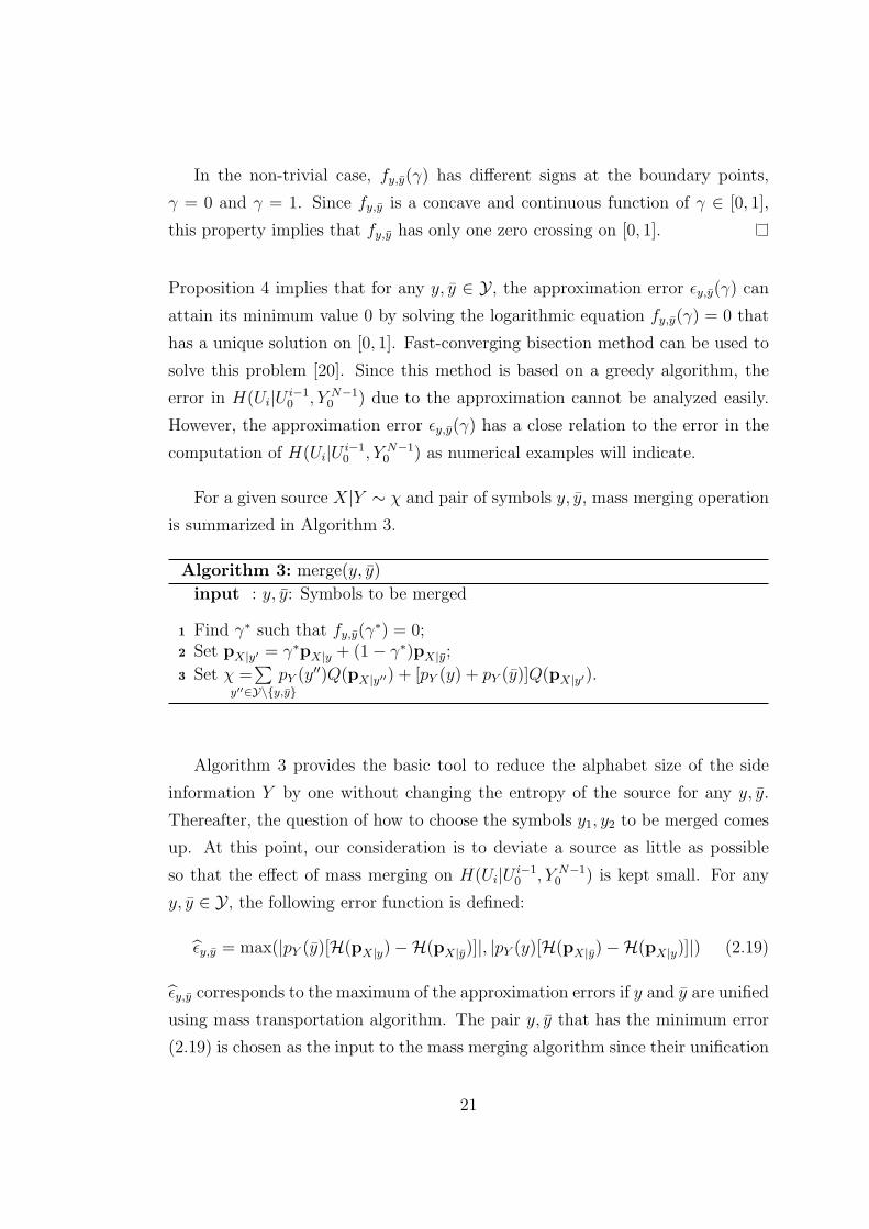
For a given source X|Y ∼ χ and pair of symbols y, y, mass merging operation
is summarized in Algorithm 3.
Algorithm 3: merge(y, y)
input : y, y: Symbols to be merged
1 Find γ∗ such that fy,y(γ∗) = 0;
2 Set pX|y′ = γ∗pX|y + (1− γ∗)pX|y;
3 Set χ =∑
y′′∈Y\{y,y}
pY (y′′)Q(pX|y′′) + [pY (y) + pY (y)]Q(pX|y′).
Algorithm 3 provides the basic tool to reduce the alphabet size of the side
information Y by one without changing the entropy of the source for any y, y.
Thereafter, the question of how to choose the symbols y1, y2 to be merged comes
up. At this point, our consideration is to deviate a source as little as possible
so that the effect of mass merging on H(Ui|Ui−10 , Y N−1
0 ) is kept small. For any
y, y ∈ Y , the following error function is defined:
ǫy,y = max(|pY (y)[H(pX|y)−H(pX|y)]|, |pY (y)[H(pX|y)−H(pX|y)]|) (2.19)
ǫy,y corresponds to the maximum of the approximation errors if y and y are unified
using mass transportation algorithm. The pair y, y that has the minimum error
(2.19) is chosen as the input to the mass merging algorithm since their unification
21

is likely to affect H(Ui|Ui−10 , Y N−1
0 ) minimally. Therefore, for each y ∈ Y , the
pair is defined as follows:
π(y) = argminy∈Y\{y}
ǫy,y (2.20)
Given X|Y ∼ χ, the following symbol y is chosen for merging together with its
pair π(y):
y = argminy∈Y
ǫy,π(y) (2.21)
Since the greedy approximation method calls the mass merging function succes-
sively, the above procedure for finding the most appropriate pair of symbols for
merging is inefficient. In order to improve efficiency at the expense of a slight
performance degradation, the following procedure, an extension of the approach
in [14], can be applied:
• Sort (pY (yi),pX|yi) such that H(pX|yi
) ≤ H(pX|yi+1) for all i ∈
{0, 1, . . . , |Y| − 1},
• Compute ǫyi,yi+1for all i,
• Choose yi, yi+1 that has minimum ǫyi,yi+1for mass merging.
In this approach, ǫyi,yi+1values can be computed once, and after each application
of the merge(y, yi+1) function, ǫyi−1,yi and ǫyi,yi+1are updated. In Algorithm 4, the
greedy mass merging function that follows the second approach is summarized.
Combining the mass merging algorithm with the code construction scheme
(2.14), the efficient polar code construction algorithm is implemented as in Algo-
rithm 5.
Using mass merging algorithm with parameter µ on χ(k)i , the size of χ
(k+1)i
is bounded above by µ2q, which follows from (2.14). Therefore, complexity is
controlled through the polar transform. Since the size of χ(k)i , k = 1, . . . , n
changes through polar transform and mass merging, a modified doubly linked list
data structure is proposed in [14], and computational complexity of the algorithm
is found as O(µ2 log µ). Similar data structures can be utilized to implement the
greedy code construction algorithm proposed in this subsection.
22
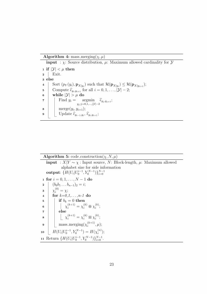
Algorithm 4: mass merging(χ, µ)
input : χ: Source distribution, µ: Maximum allowed cardinality for Y
1 if |Y| < µ then
2 Exit.3 else
4 Sort (pY (yi),pX|yi) such that H(pX|yi
) ≤ H(pX|yi+1);
5 Compute ǫyi,yi+1for all i = 0, 1, . . . , |Y| − 2;
6 while |Y| > µ do
7 Find yi = argminyj :j=0,1,...,|Y|−2
ǫyj ,yj+1;
8 merge(yi, yi+1);9 Update ǫyi−1,yi , ǫyi,yi+1
;
Algorithm 5: code construction(χ,N, µ)
input : X|Y ∼ χ : Input source, N : Block-length, µ: Maximum allowedalphabet size for side information
output: {H(Ui|Ui−10 , Y N−1
0 )}N−1i=0
1 for i = 0, 1, . . . , N − 1 do
2 (b0b1 . . . bn−1)2 = i;
3 χ(0)i = χ;
4 for k=0,1,. . . ,n-1 do
5 if bk = 0 then
6 χ(k+1)i = χ
(k)i � χ
(k)i ;
7 else
8 χ(k+1)i = χ
(k)i � χ
(k)i ;
9 mass merging(χ(k+1)i , µ);
10 H(Ui|Ui−10 , Y N−1
0 ) = H(χ(n)i );
11 Return {H(Ui|Ui−10 , Y N−1
0 )}N−1i=0 .
23
2.5 Numerical Results
In this section, the performance of the proposed data compression scheme is
investigated. The figures of merit in this investigation are the block error rate
Pb and symbol error rate Ps for a fixed code rate R. Code constructions in all
examples are performed with mass merging algorithm with parameter µ = 16.
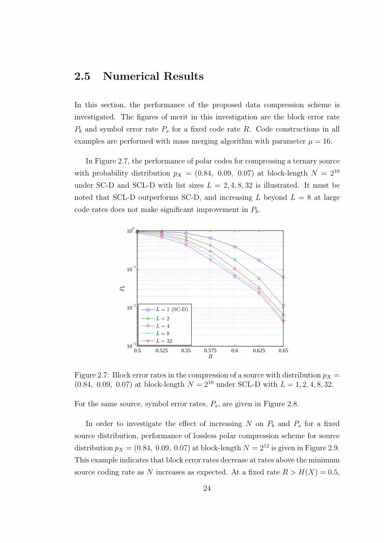
In Figure 2.7, the performance of polar codes for compressing a ternary source
with probability distribution pX = (0.84, 0.09, 0.07) at block-length N = 210
under SC-D and SCL-D with list sizes L = 2, 4, 8, 32 is illustrated. It must be
noted that SCL-D outperforms SC-D, and increasing L beyond L = 8 at large
code rates does not make significant improvement in Pb.
0.5 0.525 0.55 0.575 0.6 0.625 0.6510
−3
10−2
10−1
100
R
Pb
L = 1 (SC-D)
L = 2
L = 4
L = 8
L = 32
Figure 2.7: Block error rates in the compression of a source with distribution pX =(0.84, 0.09, 0.07) at block-length N = 210 under SCL-D with L = 1, 2, 4, 8, 32.
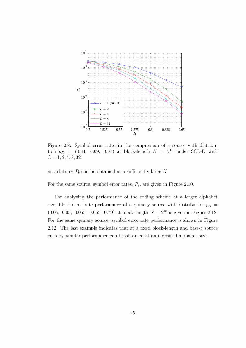
For the same source, symbol error rates, Ps, are given in Figure 2.8.
In order to investigate the effect of increasing N on Pb and Ps for a fixed
source distribution, performance of lossless polar compression scheme for source
distribution pX = (0.84, 0.09, 0.07) at block-lengthN = 212 is given in Figure 2.9.
This example indicates that block error rates decrease at rates above the minimum
source coding rate as N increases as expected. At a fixed rate R > H(X) = 0.5,
24
0.5 0.525 0.55 0.575 0.6 0.625 0.6510
−5
10−4
10−3
10−2
10−1
100
R
Ps
L = 1 (SC-D)
L = 2
L = 4
L = 8
L = 32
Figure 2.8: Symbol error rates in the compression of a source with distribu-tion pX = (0.84, 0.09, 0.07) at block-length N = 210 under SCL-D withL = 1, 2, 4, 8, 32.
an arbitrary Pb can be obtained at a sufficiently large N .
For the same source, symbol error rates, Ps, are given in Figure 2.10.
For analyzing the performance of the coding scheme at a larger alphabet
size, block error rate performance of a quinary source with distribution pX =
(0.05, 0.05, 0.055, 0.055, 0.79) at block-length N = 210 is given in Figure 2.12.
For the same quinary source, symbol error rate performance is shown in Figure
2.12. The last example indicates that at a fixed block-length and base-q source
entropy, similar performance can be obtained at an increased alphabet size.
25
0.5 0.525 0.55 0.575 0.6 0.62510
−4
10−3
10−2
10−1
100
R
Pb
L = 1 (SC-D)
L = 2
L = 4
L = 8
L = 32
Figure 2.9: Block error rates in the compression of a source with distribution pX =(0.84, 0.09, 0.07) at block-length N = 212 under SCL-D with L = 1, 2, 4, 8, 32.
0.5 0.525 0.55 0.575 0.6 0.625 0.6510
−6
10−5
10−4
10−3
10−2
10−1
100
R
Ps
L = 1 (SC-D)
L = 2
L = 4
L = 8
L = 32
Figure 2.10: Symbol error rates in the compression of a source with distri-bution pX = (0.84, 0.09, 0.07) at block-length N = 212 under SCL-D withL = 1, 2, 4, 8, 32.
26
0.5 0.525 0.55 0.575 0.6 0.625 0.6510
−3
10−2
10−1
100
R
Pb
L = 1 (SC-D)
L = 2
L = 4
L = 8
L = 32
Figure 2.11: Block error rates in the compression of a source with distributionpX = (0.05, 0.05, 0.055, 0.055, 0.79) at block-length N = 210 under SCL-D withL = 1, 2, 4, 8, 32.
0.5 0.525 0.55 0.575 0.6 0.625 0.6510
−5
10−4
10−3
10−2
10−1
100
R
Ps
L = 1 (SC-D)
L = 2
L = 4
L = 8
L = 32
Figure 2.12: Symbol error rates in the compression of a source with distributionpX = (0.05, 0.05, 0.055, 0.055, 0.79) at block-length N = 212 under SCL-D withL = 1, 2, 4, 8, 32.
27
Chapter 3
Oracle-Based Lossless Polar
Compression
3.1 Introduction
In Chapter 2, in order to compress a sequence {(Xi, Yi)}N−1i=0 , an informa-
tion set IX|Y (N,R) consisting of indices i that correspond to NR highest
H(Ui|Ui−10 , Y N−1
0 ) terms is constructed. Then, a given realization xN−10 is trans-
formed into uN−10 by (2.2) and the compressed word uIX|Y
is formed. For suffi-
ciently large N , this scheme is proved to achieve arbitrarily small probability of
error under conventional SC-D with codeword length NH(X|Y ) [8]. In [9], for
binary sources, an oracle-based polar compression method that has an improved
performance at finite block-lengths is introduced. Here, a similar approach is
taken in the design of fixed-to-variable length, zero-error compression methods
for q-ary discrete memoryless sources. The methods are based on appending a
block, namely oracle set T , to the compressed word uIX|Yindicating the loca-
tions of the errors that will be encountered in decoding, and correcting them.
This block enables zero-error coding at any block-length. Moreover, it is shown
that this extra block has a diminishing fraction in the transmitted word, which
means that the minimum source coding rate is still achievable asymptotically in
28
the block-length. The discussion in this chapter is partly presented in [21].
3.2 Preliminaries
For finite-length analysis and code construction, the minimal error probability,
analyzed in [22], provides a more convenient measure than conditional entropy
[9]. The minimal error probability, denoted by π(X|Y = y), is the probability of
error in the maximum a posteriori estimation of X given an observation Y = y:
π(X|Y = y) = Pr[X 6= argmaxx∈X
pX|Y (x|y)|Y = y],
= 1−maxx∈X
pX|Y (x|y).
Therefore, the average minimal probability of error is as follows:
π(X|Y ) =∑
y∈Y
pY (y)π(X|Y = y). (3.1)
π(X|Y ) has a range [0, q−1q] and is a concave function of pX|Y (x|y).
3.3 Encoding
In noiseless source coding, the encoder has a copy of the codeword received by
the decoder. This specific property enables the encoder to run the decoder at the
transmitter side and check if a decoding error occurs. In polar compression, this
capability can be utilized to prevent any errors by appending a variable length
block of error positions and their correct symbols to the codeword; thus fixed-
to-variable length, zero-error coding schemes can be designed. The oracle-based
lossless polar compression scheme with successive cancellation type decoders is
illustrated in Figure 3.1.
The encoding is specific to the type of decoder. Therefore, we will consider
schemes with SC-D and SCL-D separately. First, let us consider the encoding in
the case of SC-D, which is a straightforward extension of [9].
29
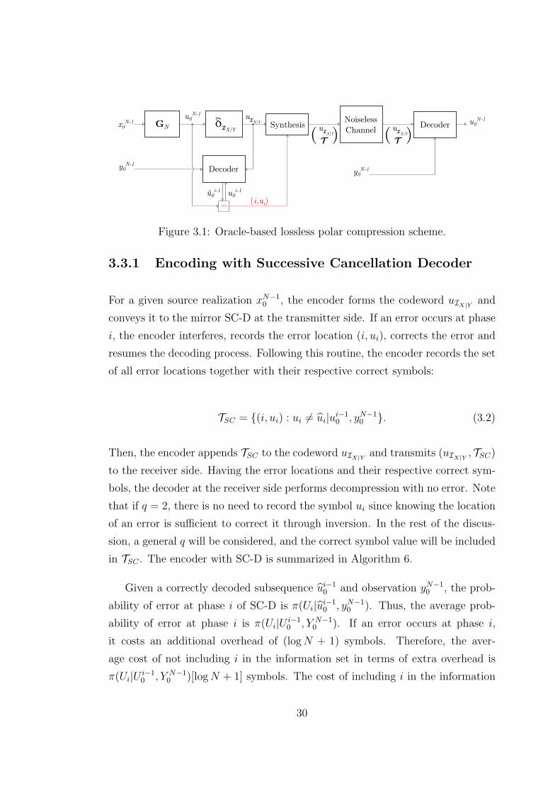
Figure 3.1: Oracle-based lossless polar compression scheme.
3.3.1 Encoding with Successive Cancellation Decoder
For a given source realization xN−10 , the encoder forms the codeword uIX|Y
and
conveys it to the mirror SC-D at the transmitter side. If an error occurs at phase
i, the encoder interferes, records the error location (i, ui), corrects the error and
resumes the decoding process. Following this routine, the encoder records the set
of all error locations together with their respective correct symbols:
TSC = {(i, ui) : ui 6= ui|ui−10 , yN−1
0 }. (3.2)
Then, the encoder appends TSC to the codeword uIX|Yand transmits (uIX|Y
, TSC)
to the receiver side. Having the error locations and their respective correct sym-
bols, the decoder at the receiver side performs decompression with no error. Note
that if q = 2, there is no need to record the symbol ui since knowing the location
of an error is sufficient to correct it through inversion. In the rest of the discus-
sion, a general q will be considered, and the correct symbol value will be included
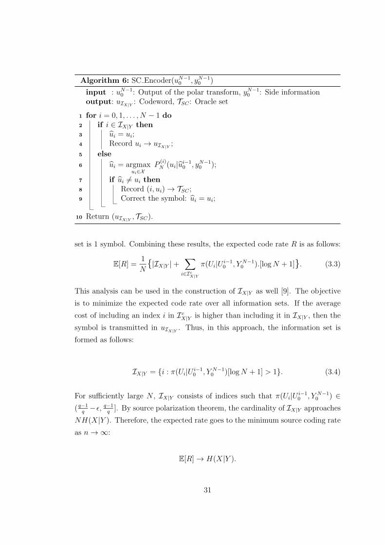
in TSC . The encoder with SC-D is summarized in Algorithm 6.
Given a correctly decoded subsequence ui−10 and observation yN−1
0 , the prob-
ability of error at phase i of SC-D is π(Ui|ui−10 , yN−1
0 ). Thus, the average prob-
ability of error at phase i is π(Ui|Ui−10 , Y N−1
0 ). If an error occurs at phase i,
it costs an additional overhead of (logN + 1) symbols. Therefore, the aver-
age cost of not including i in the information set in terms of extra overhead is
π(Ui|Ui−10 , Y N−1
0 )[logN + 1] symbols. The cost of including i in the information
30
Algorithm 6: SC Encoder(uN−10 , yN−1
0 )
input : uN−10 : Output of the polar transform, yN−1
0 : Side informationoutput: uIX|Y
: Codeword, TSC : Oracle set
1 for i = 0, 1, . . . , N − 1 do
2 if i ∈ IX|Y then
3 ui = ui;4 Record ui → uIX|Y
;
5 else
6 ui = argmaxui∈X
P(i)N (ui|u
i−10 , yN−1
0 );
7 if ui 6= ui then
8 Record (i, ui) → TSC ;9 Correct the symbol: ui = ui;
10 Return (uIX|Y, TSC).
set is 1 symbol. Combining these results, the expected code rate R is as follows:
E[R] =1
N{|IX|Y |+
∑
i∈IcX|Y
π(Ui|Ui−10 , Y N−1
0 ).[logN + 1]}. (3.3)
This analysis can be used in the construction of IX|Y as well [9]. The objective
is to minimize the expected code rate over all information sets. If the average
cost of including an index i in IcX|Y is higher than including it in IX|Y , then the
symbol is transmitted in uIX|Y. Thus, in this approach, the information set is
formed as follows:
IX|Y = {i : π(Ui|Ui−10 , Y N−1
0 )[logN + 1] > 1}. (3.4)
For sufficiently large N , IX|Y consists of indices such that π(Ui|Ui−10 , Y N−1
0 ) ∈
( q−1q
−ǫ, q−1q]. By source polarization theorem, the cardinality of IX|Y approaches
NH(X|Y ). Therefore, the expected rate goes to the minimum source coding rate
as n → ∞:
E[R] → H(X|Y ).
31
Hence, this zero-error compression scheme designed for finite block-lengths
achieves the theoretical bound asymptotically as well.
The following question arises: How to compute {π(Ui|Ui−10 , Y N−1
0 )}N−1i=0 to
construct IX|Y using (3.4)? By (3.1), the set of (q + 1)-dimensional vectors
{(pY (y), [pX|Y (x|y)]q−1x=0)}y∈Y is required for this computation, which implies that
Ui|Ui−10 , Y N−1
0 is required to compute π(Ui|Ui−10 , Y N−1
0 ) similar to the case of
conditional entropy. Therefore, a slight modification in the code construction
method proposed in Section 2.4 suffices for code construction in this case. One
alternative for this modification is to replace H by π in (2.17) and perform mass
merging using average minimal error probability. Since π is a concave function
of p, this alternative works. The other alternative is to perform code construc-
tion in the same way as Chapter 2 until Line 10 of Algorithm 5 and computing
π(Ui|Ui−10 , Y N−1
0 ) from χ(n)i .
3.3.2 Encoding with Successive Cancellation List Decoder
The SC-D flags a block error once an incorrect decision is made and causes ad-
ditional overhead because of oracle employment. Successive cancellation list de-
coder is likely to correct an incorrect decision at succeeding phases in the expense
of increased complexity. In noiseless source coding, this property of SCL-D can
be utilized to reduce the expected codeword length. Consider an SCL-D of list
size L at phase i /∈ IX|Y . Assume that the correct decoding path ui−10 = ui−1
0 is
contained among the active paths. At phase i, all symbols in X is appended to
each active path, and all paths are pruned keeping L of the highest probability
values. Denoting the set of all active paths at phase i by Li, an error is flagged
if the correct subsequence ui0 is not in Li. If such an event occurs, the encoder
interferes, takes a record of (i, ui) and appends ui to each active path as if i is
contained in the information set. Eventually, the oracle set is formed as follows:
TSCL = {(i, ui) : ui0 /∈ Li|u
i−10 ∈ Li−1, y
N−10 }. (3.5)
The employment of this oracle set guarantees the correct decoding path uN−10
32
to survive until the end. In the last phase, SCL-D returns the sequence among
LN−1 with highest probability. An incorrect sequence is returned if there is a
path uN−10 ∈ LN−1 with higher probability than uN−1
0 . In order to prevent this
error, the list index l of the correct sequence can be annexed to the codeword.
This increases the codeword length by logL symbols. On the other hand, since
the probability of error event, Pr{ui0 /∈ Li|y
N−10 }, is smaller than the probability
of error event in SC-D, Pr{ui 6= ui|ui−10 = ui−1
0 , yN−10 }, and hence the use of
the oracle becomes less frequent, the overall overhead decreases compared to the
oracle-based compression scheme with SC-D.
3.4 Decoding
In this section, oracle decoders that reconstruct xN−10 from uIX|Y
and oracle set
T will be proposed. The decoders are basically similar to the ones discussed in
Chapter 2 with the difference that oracle sets are also exploited for zero-error
reconstruction.
3.4.1 Successive Cancellation Decoder for Oracle-Based
Compression
For a given source (X, Y ) and observation yN−10 , the probability of observing uN−1
0
at the output of the polarization transform is denoted as PN(uN−10 |yN−1
0 ), where
P1(x|y) = pX(x|y). Similarly, the probability of a subsequence ui0 is denoted as
P(i)N (ui|u
i−10 , yN−1
0 ). SC-D algorithm is summarized in Algorithm 7.
SC-D can be implemented with O(N) memory and O(N logN) run-time com-
plexity [17].
33
Algorithm 7: SC Decoder(uIX|Y, yN−1
0 , TSC)
input : uIX|Y: Codeword, yN−1
0 : Side information, TSC : Oracle set
output: xN−10 : Reconstructed sequence
1 for i = 0, 1, . . . , N − 1 do
2 if i ∈ IX|Y or (i, ui) ∈ TSC then
3 ui = ui
4 else
5 ui = argmaxui∈X
P(i)N (ui|u
i−10 , yN−1
0 );
6 Return xN−10 = uN−1
0 G−1N .
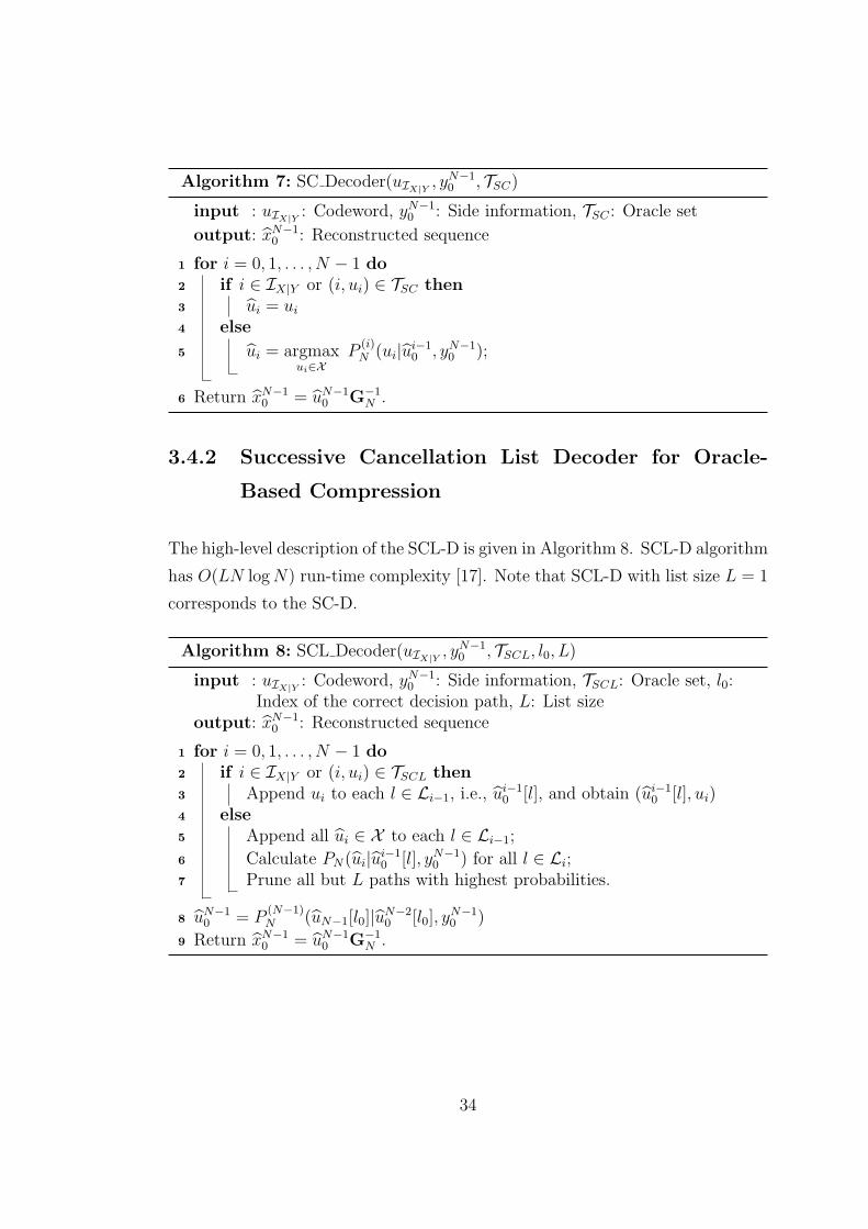
3.4.2 Successive Cancellation List Decoder for Oracle-
Based Compression
The high-level description of the SCL-D is given in Algorithm 8. SCL-D algorithm
has O(LN logN) run-time complexity [17]. Note that SCL-D with list size L = 1
corresponds to the SC-D.
Algorithm 8: SCL Decoder(uIX|Y, yN−1
0 , TSCL, l0, L)
input : uIX|Y: Codeword, yN−1
0 : Side information, TSCL: Oracle set, l0:Index of the correct decision path, L: List size
output: xN−10 : Reconstructed sequence
1 for i = 0, 1, . . . , N − 1 do
2 if i ∈ IX|Y or (i, ui) ∈ TSCL then
3 Append ui to each l ∈ Li−1, i.e., ui−10 [l], and obtain (ui−1
0 [l], ui)4 else
5 Append all ui ∈ X to each l ∈ Li−1;
6 Calculate PN(ui|ui−10 [l], yN−1
0 ) for all l ∈ Li;7 Prune all but L paths with highest probabilities.
8 uN−10 = P
(N−1)N (uN−1[l0]|u
N−20 [l0], y
N−10 )
9 Return xN−10 = uN−1
0 G−1N .
34
3.5 Compression of Sources over Arbitrary Fi-
nite Alphabets
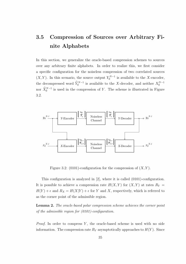
In this section, we generalize the oracle-based compression schemes to sources
over any arbitrary finite alphabets. In order to realize this, we first consider
a specific configuration for the noiseless compression of two correlated sources
(X, Y ). In this scenario, the source output Y N−10 is available to the X-encoder,
the decompressed word Y N−10 is available to the X-decoder, and neither XN−1
0
nor XN−10 is used in the compression of Y . The scheme is illustrated in Figure
3.2.
Figure 3.2: (0101)-configuration for the compression of (X, Y ).
This configuration is analyzed in [2], where it is called (0101)-configuration.
It is possible to achieve a compression rate H(X, Y ) for (X, Y ) at rates RY =
H(Y ) + ǫ and RX = H(X|Y ) + ǫ for Y and X, respectively, which is referred to
as the corner point of the admissible region.
Lemma 2. The oracle-based polar compression scheme achieves the corner point
of the admissible region for (0101)-configuration.
Proof. In order to compress Y , the oracle-based scheme is used with no side
information. The compression rate RY asymptotically approaches toH(Y ). Since
35
this is a zero-error coding scheme, the Y -source output is reconstructed faithfully
at the receiver side. In order to compress X, the oracle-based compression scheme
is used with the side information Y . Note that Y -source output is available at
both transmitter and receiver sides with no error. Thus, X can be compressed
at rate RX = H(X|Y ) with the oracle described in (3.2), and the corner point of
(0101)-configuration is achieved asymptotically.
An extension of this configuration is the noiseless source coding over arbitrary
finite alphabets, using a similar approach as in [16]. Let Z be a random variable
over a finite alphabet Z. Z can be decomposed into K symbols using the Chinese
remainder theorem as:
Z = (ZK−1, ZK−2, . . . , Z0),
where Zk is over Zk, provided that |Zk| = qk and all qk are pairwise coprime.
Note that qk can be an integer power of a prime, in which a further expansion
can be carried out to obtain prime alphabet sizes for compression, and the result
can be used to uniquely reconstruct Z. Hence, without loss of generality, it can
be assumed in further discussions that all qk are prime.
At the first step of compressing Z, Z0 is compressed with no side informa-
tion, analogous to Y in the previous case, at rate approximately equal to H(Z0).
Then, Z1 is compressed with side information Z0 at rate approximately equal to
H(Z1|Z0). Now that the source outputs of (Z1, Z0) are transmitted, they are
utilized as side information and the compression of Z2 is performed at rate ap-
proximately equal to H(Z2|Z1, Z0). Following this routine, Zk can be compressed
at rate H(Zk|Zk−1, . . . , Z0) for any k = 0, 1, . . . , K − 1. After the decompression
of ZK−1, Z can be reconstructed faithfully. The total compression in this scheme
has the following asymptotical rate:
RZ =K−1∑
k=0
RZk
→K−1∑
k=0
H(Zk|Zk−1, . . . , Z0)
= H(ZK−1, ZK−2, . . . , Z0) = H(Z),
36
which shows that the entropy bound can be achieved asymptotically by the pro-
posed q-ary polar compression scheme.
In the general case, assume that the alphabet size is q =K−1∏k=0
qtkk for pairwise
coprimes qk and positive integers tk for all k = 0, 1, . . . , K − 1. In this case, for
a list size L and block-length N , the complexity of the multi-level compression
scheme is O(K−1∑k=0
tkqkLN logN). Therefore, it is possible to perform data com-
pression for large source alphabets at low complexity by the multi-level scheme.
3.6 Source Distribution Uncertainty at the Re-
ceiver
In the previous sections, it was assumed that the exact probability distribution of
the source, denoted as pX in the q-dimensional vector form, is available at the re-
ceiver, and the information set, denoted as IX(pX , N), is constructed specifically
for pX . In practice, however, these assumptions are unrealistic since the receiver
does not have pX unless it is informed by the transmitter side. Moreover, even
if the exact knowledge of pX is available at the transmitter, it is infeasible to
construct IX specifically for every given pX . In this section, we propose methods
to address these issues by exploiting robustness of the oracle-based polar com-
pression scheme with respect to the inaccuracies in the source distribution and
information set. We consider only data compression in the absence of side infor-
mation in this section, and the alphabet size is q for a prime integer q. We note
that it is straightforward to extend the presented results to the case with side
information and non-prime alphabet sizes.
Throughout the section, following the notation in [15], M(q) denotes the set
of all probability distributions on a q-ary alphabet:
M(q) = {p ∈ Rq : pi > 0 for all i ∈ {0, 1, . . . , q − 1},
q−1∑i=0
pi = 1}.
37
For given pX ,pY ∈ M(q), if there exists pZ ∈ M(q) such that pY = pX ∗ pZ
where ∗ denotes circular convolution [23], pY is said to be circularly dominated
by pX , and this relation is represented as pY ≺c pX .
First, we propose a method to inform the receiver about the probability dis-
tribution of the source pX efficiently in the oracle-based framework. In order to
inform the receiver side about pX , our approach is to quantize q − 1 elements of
pX by using β symbols, and append the quantized probability distribution pX to
the compressed word.
3.6.1 Sequential Quantization with Scaling Algorithm for
Probability Mass Functions
For the quantization of a probility distribution pX , sequential quantization with
scaling provides an efficient solution. In this quantization approach, the original
probability distribution is sorted in the descending order, i.e., a permutation
transformation φ : M(q) 7→ M(q) must be applied such that p = φ(pX) where
p0 ≥ p1 ≥ . . . ≥ pq−1 holds between the elements of p. Note that the permutation
φ can be transmitted to the receiver by q − 1 symbols, which implies that the
original ordering of the elements of pX can be restored at the receiver with no
loss of fidelity.
For a probability distribution function p, the sorted order implies the following
bounds for the value of pi:
pi ∈ [
1−i−1∑k=0
pk
q − i, 1−
i−1∑
k=0
pk]. (3.6)
The sequential quantization with scaling algorithm starts with the quantization
of p0, and then the bounds in (3.6) are found for each pi, i = 0, 1, . . . , q − 1 by
using the previously quantized elements pi−10 , and the interval in (3.6) is divided
into qβ uniform levels. The level di ∈ {0, 1, . . . , qβ − 1} that provides the best
approximation to pi is chosen for the compressed word in its q-ary expansion.
38
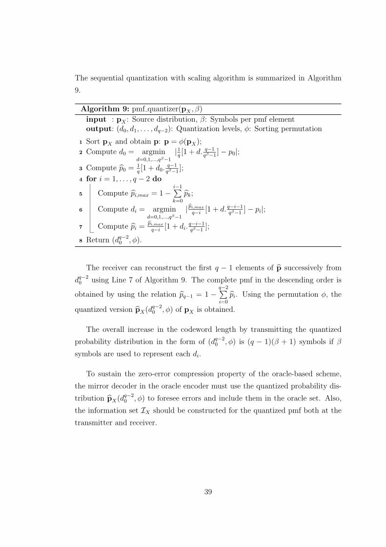
The sequential quantization with scaling algorithm is summarized in Algorithm
9.
Algorithm 9: pmf quantizer(pX , β)
input : pX : Source distribution, β: Symbols per pmf elementoutput: (d0, d1, . . . , dq−2): Quantization levels, φ: Sorting permutation
1 Sort pX and obtain p: p = φ(pX);
2 Compute d0 = argmind=0,1,...,qβ−1
|1q[1 + d. q−1
qβ−1]− p0|;
3 Compute p0 =1q[1 + d0.
q−1qβ−1
];
4 for i = 1, . . . , q − 2 do
5 Compute pi,max = 1−i−1∑k=0
pk;
6 Compute di = argmind=0,1,...,qβ−1
|pi,max
q−i[1 + d. q−i−1
qβ−1]− pi|;
7 Compute pi =pi,max
q−i[1 + di.
q−i−1qβ−1
];
8 Return (dq−20 , φ).
The receiver can reconstruct the first q − 1 elements of p successively from
dq−20 using Line 7 of Algorithm 9. The complete pmf in the descending order is
obtained by using the relation pq−1 = 1 −q−2∑i=0
pi. Using the permutation φ, the
quantized version pX(dq−20 , φ) of pX is obtained.
The overall increase in the codeword length by transmitting the quantized
probability distribution in the form of (dq−20 , φ) is (q − 1)(β + 1) symbols if β
symbols are used to represent each di.
To sustain the zero-error compression property of the oracle-based scheme,
the mirror decoder in the oracle encoder must use the quantized probability dis-
tribution pX(dq−20 , φ) to foresee errors and include them in the oracle set. Also,
the information set IX should be constructed for the quantized pmf both at the
transmitter and receiver.
39
3.6.2 Information Sets under Source Uncertainty and the
Concept of Class of Information Sets
The computation of {π(Ui|Ui−10 )}N−1
i=0 using density evolution algorithm with the
q-ary extension of the approximation methods proposed in [14] has run-time com-
plexity of O(N). However, for accurate approximations, the approximation pa-
rameter of the greedy algorithm µ must be chosen sufficiently large as the al-
phabet size q increases. Considering that the algorithmic complexity of the code
construction algorithm O(µ2 log µ), constructing the information set IX by using
density evolution technique for every given source is infeasible in practice. To
overcome this problem, we propose using a class of pre-built information sets.
In the following, the concept of class of information sets (CIS) will be defined
first, and then a CIS construction technique for the source polarization will be
proposed by investigating robustness of the compression scheme with respect to
the perturbations in the information set.
Definition 1. For a given block-length N = 2n, a positive integer C, and a set of
probability distributions pi ∈ M(q) for i = 0, 1, . . . , C−1, the class of information
set (CIS)
C = {IX(pi, N), i = 0, 1, . . . , C − 1}
is a pre-built class of index sets which is known at both the transmitter and the
receiver, together with the corresponding probability distributions pi.
For a given realization xN−10 drawn from a probability distribution pX whose
β-symbol quantized version is pX , the CIS C is used as follows:
1. The transmitter finds pi such that using IX(pi, N) ∈ C minimizes the code
rate, and uses this information set to form the codeword (uIX , T , dq−20 , φ).
2. After the receiver reconstructs pX , it finds pi in the same way as the trans-
mitter, and uses the corresponding information set in the recontruction of
xN−10 .
40
In order to measure the robustness of the lossless polar compression scheme
with respect to inaccuracies in the information set, we consider the average in-
crease in the length of the compressed word if an information set constructed
for a different probability distribution than the source distribution is used. Let
pX ∈ M(q) be the probability distribution of the source XN−10 and p be an
arbitrary distribution over M(q). The average cost of using IX(p, N) in the
compression of XN−10 is defined as follows:
JN(pX ,p) = E[R(IX(p, N))|pX ]− E[R(IX(pX , N))|pX ], (3.7)
where E[R(IX)|pX ] is the average code rate if the source distribution is pX and
information set IX is used in the compression.
Proposition 5. For a given source XN−10 ∼ pX ∈ M(q) and p ∈ M(q), the cost
function in (3.7) can be computed as follows:
JN(pX ,p) =N−1∑
i=0
π(Ui|Ui−10 )[logN + 1]− 1
N.ωi, (3.8)
where {π(Ui|Ui−10 )}N−1
i=0 } is the set of average minimal error probabilities for
XN−10 , and
ωi =
1 i ∈ IX(pX , N) ∩ IX(p, N)c,
−1 i ∈ IX(pX , N)c ∩ IX(p, N),
0 otherwise.
The proof simply follows from (3.3). Since only IX(pX , N) can be used at the
receiver side, replacement of JN(pX ,p) by JN(pX ,p) provides a more appropriate
analysis given that β is large enough for accurate β-symbol quantization.
3.6.2.1 A CIS Construction Scheme
Proposition 5 provides a useful tool for investigating robustness of polar com-
pression scheme and constructing CIS. Spike probability distributions defined in
[15] are of particular interest for constructing CIS because of the design simplicity
they provide and numerical stability considerations. For constructing information
41
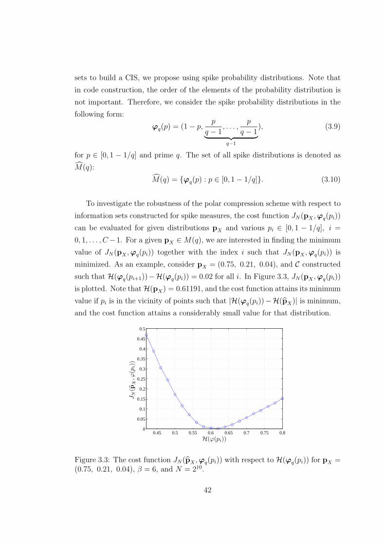
sets to build a CIS, we propose using spike probability distributions. Note that
in code construction, the order of the elements of the probability distribution is
not important. Therefore, we consider the spike probability distributions in the
following form:
ϕq(p) = (1− p,p
q − 1, . . . ,
p
q − 1︸ ︷︷ ︸q−1
), (3.9)
for p ∈ [0, 1 − 1/q] and prime q. The set of all spike distributions is denoted as
M(q):
M(q) = {ϕq(p) : p ∈ [0, 1− 1/q]}. (3.10)
To investigate the robustness of the polar compression scheme with respect to
information sets constructed for spike measures, the cost function JN(pX ,ϕq(pi))
can be evaluated for given distributions pX and various pi ∈ [0, 1 − 1/q], i =
0, 1, . . . , C−1. For a given pX ∈ M(q), we are interested in finding the minimum
value of JN(pX ,ϕq(pi)) together with the index i such that JN(pX ,ϕq(pi)) is
minimized. As an example, consider pX = (0.75, 0.21, 0.04), and C constructed
such that H(ϕq(pi+1))−H(ϕq(pi)) = 0.02 for all i. In Figure 3.3, JN(pX ,ϕq(pi))
is plotted. Note thatH(pX) = 0.61191, and the cost function attains its minimum
value if pi is in the vicinity of points such that |H(ϕq(pi))−H(pX)| is minimum,
and the cost function attains a considerably small value for that distribution.
0.45 0.5 0.55 0.6 0.65 0.7 0.75 0.80
0.05
0.1
0.15
0.2
0.25
0.3
0.35
0.4
0.45
0.5
JN
(pX
,ϕ(p
i))
H(ϕ(pi))
Figure 3.3: The cost function JN(pX ,ϕq(pi)) with respect to H(ϕq(pi)) for pX =(0.75, 0.21, 0.04), β = 6, and N = 210.
42
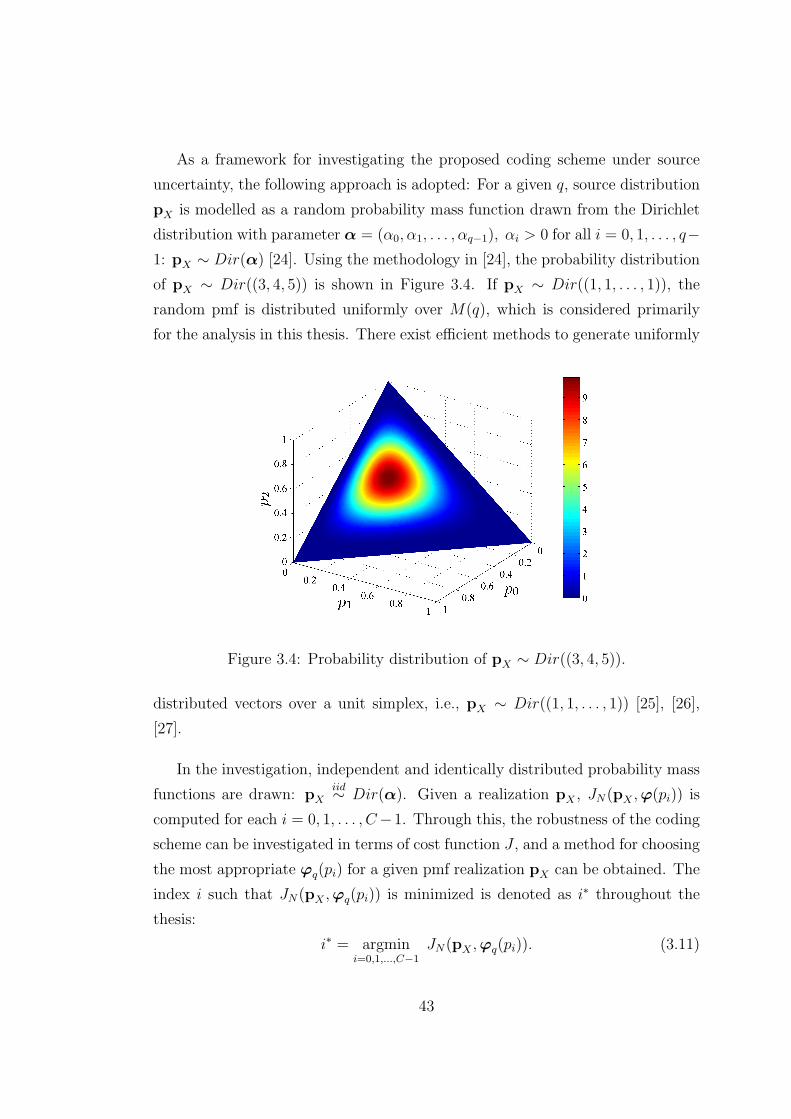
As a framework for investigating the proposed coding scheme under source
uncertainty, the following approach is adopted: For a given q, source distribution
pX is modelled as a random probability mass function drawn from the Dirichlet
distribution with parameter α = (α0, α1, . . . , αq−1), αi > 0 for all i = 0, 1, . . . , q−
1: pX ∼ Dir(α) [24]. Using the methodology in [24], the probability distribution
of pX ∼ Dir((3, 4, 5)) is shown in Figure 3.4. If pX ∼ Dir((1, 1, . . . , 1)), the
random pmf is distributed uniformly over M(q), which is considered primarily
for the analysis in this thesis. There exist efficient methods to generate uniformly
Figure 3.4: Probability distribution of pX ∼ Dir((3, 4, 5)).
distributed vectors over a unit simplex, i.e., pX ∼ Dir((1, 1, . . . , 1)) [25], [26],
[27].
In the investigation, independent and identically distributed probability mass
functions are drawn: pXiid∼ Dir(α). Given a realization pX , JN(pX ,ϕ(pi)) is
computed for each i = 0, 1, . . . , C−1. Through this, the robustness of the coding
scheme can be investigated in terms of cost function J , and a method for choosing
the most appropriate ϕq(pi) for a given pmf realization pX can be obtained. The
index i such that JN(pX ,ϕq(pi)) is minimized is denoted as i∗ throughout the
thesis:
i∗ = argmini=0,1,...,C−1
JN(pX ,ϕq(pi)). (3.11)
43
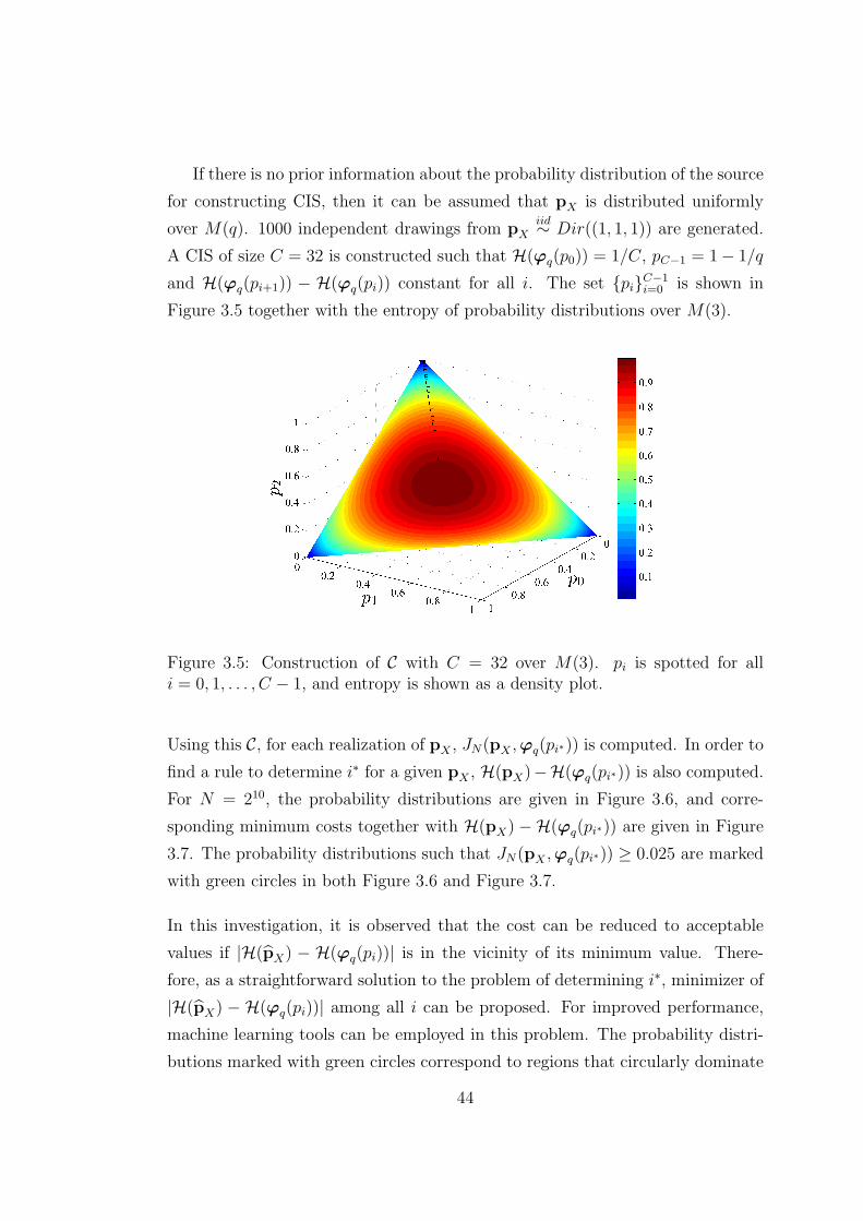
If there is no prior information about the probability distribution of the source
for constructing CIS, then it can be assumed that pX is distributed uniformly
over M(q). 1000 independent drawings from pXiid∼ Dir((1, 1, 1)) are generated.
A CIS of size C = 32 is constructed such that H(ϕq(p0)) = 1/C, pC−1 = 1− 1/q
and H(ϕq(pi+1)) − H(ϕq(pi)) constant for all i. The set {pi}C−1i=0 is shown in
Figure 3.5 together with the entropy of probability distributions over M(3).
Figure 3.5: Construction of C with C = 32 over M(3). pi is spotted for alli = 0, 1, . . . , C − 1, and entropy is shown as a density plot.
Using this C, for each realization of pX , JN(pX ,ϕq(pi∗)) is computed. In order to
find a rule to determine i∗ for a given pX , H(pX)−H(ϕq(pi∗)) is also computed.
For N = 210, the probability distributions are given in Figure 3.6, and corre-
sponding minimum costs together with H(pX)−H(ϕq(pi∗)) are given in Figure
3.7. The probability distributions such that JN(pX ,ϕq(pi∗)) ≥ 0.025 are marked
with green circles in both Figure 3.6 and Figure 3.7.
In this investigation, it is observed that the cost can be reduced to acceptable
values if |H(pX) − H(ϕq(pi))| is in the vicinity of its minimum value. There-
fore, as a straightforward solution to the problem of determining i∗, minimizer of
|H(pX) − H(ϕq(pi))| among all i can be proposed. For improved performance,
machine learning tools can be employed in this problem. The probability distri-
butions marked with green circles correspond to regions that circularly dominate
44
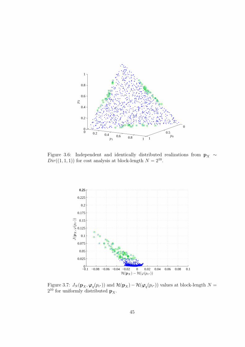
0
0.5
1
0 0.2 0.4 0.6 0.8 1
0
0.2
0.4
0.6
0.8
1p2
p1
p0
Figure 3.6: Independent and identically distributed realizations from pX ∼Dir((1, 1, 1)) for cost analysis at block-length N = 210.
−0.1 −0.08 −0.06 −0.04 −0.02 0 0.02 0.04 0.06 0.08 0.10
0.025
0.05
0.075
0.1
0.125
0.15
0.175
0.2
0.225
0.250.25
H(pX)−H(ϕ(pi∗))
J(p
X,ϕ
(pi∗))
Figure 3.7: JN(pX ,ϕq(pi∗)) and H(pX)−H(ϕq(pi∗)) values at block-length N =210 for uniformly distributed pX .
45
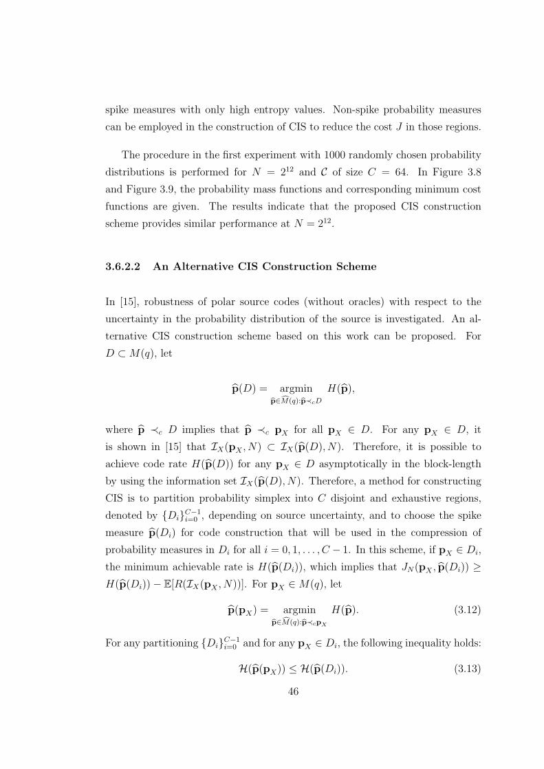
spike measures with only high entropy values. Non-spike probability measures
can be employed in the construction of CIS to reduce the cost J in those regions.
The procedure in the first experiment with 1000 randomly chosen probability
distributions is performed for N = 212 and C of size C = 64. In Figure 3.8
and Figure 3.9, the probability mass functions and corresponding minimum cost
functions are given. The results indicate that the proposed CIS construction
scheme provides similar performance at N = 212.
3.6.2.2 An Alternative CIS Construction Scheme
In [15], robustness of polar source codes (without oracles) with respect to the
uncertainty in the probability distribution of the source is investigated. An al-
ternative CIS construction scheme based on this work can be proposed. For
D ⊂ M(q), let
p(D) = argminp∈M(q):p≺cD
H(p),
where p ≺c D implies that p ≺c pX for all pX ∈ D. For any pX ∈ D, it
is shown in [15] that IX(pX , N) ⊂ IX(p(D), N). Therefore, it is possible to
achieve code rate H(p(D)) for any pX ∈ D asymptotically in the block-length
by using the information set IX(p(D), N). Therefore, a method for constructing
CIS is to partition probability simplex into C disjoint and exhaustive regions,
denoted by {Di}C−1i=0 , depending on source uncertainty, and to choose the spike
measure p(Di) for code construction that will be used in the compression of
probability measures in Di for all i = 0, 1, . . . , C − 1. In this scheme, if pX ∈ Di,
the minimum achievable rate is H(p(Di)), which implies that JN(pX , p(Di)) ≥
H(p(Di))− E[R(IX(pX , N))]. For pX ∈ M(q), let
p(pX) = argminp∈M(q):p≺cpX
H(p). (3.12)
For any partitioning {Di}C−1i=0 and for any pX ∈ Di, the following inequality holds:
H(p(pX)) ≤ H(p(Di)). (3.13)
46
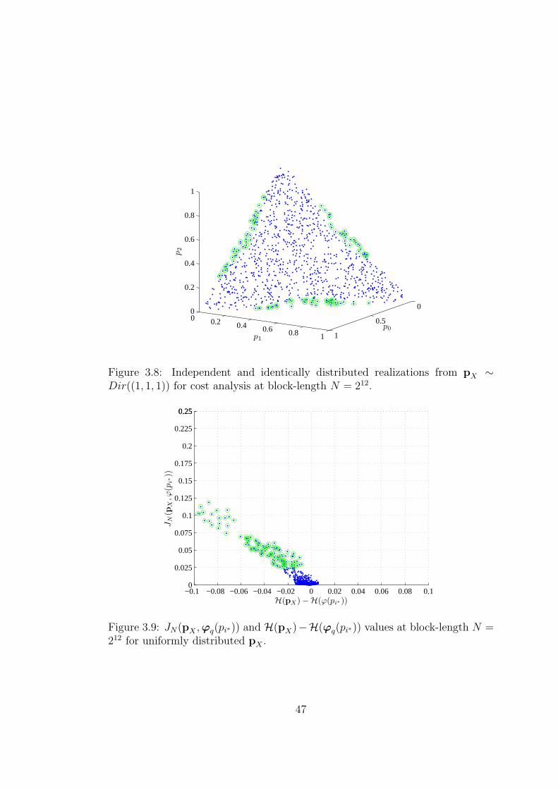
0
0.5
1
0 0.2 0.4 0.6 0.8 1
0
0.2
0.4
0.6
0.8
1
p1
p0
p2
Figure 3.8: Independent and identically distributed realizations from pX ∼Dir((1, 1, 1)) for cost analysis at block-length N = 212.
−0.1 −0.08 −0.06 −0.04 −0.02 0 0.02 0.04 0.06 0.08 0.10
0.025
0.05
0.075
0.1
0.125
0.15
0.175
0.2
0.225
0.250.25
H(pX)−H(ϕ(pi∗))
JN
(pX
,ϕ(p
i∗))
Figure 3.9: JN(pX ,ϕq(pi∗)) and H(pX)−H(ϕq(pi∗)) values at block-length N =212 for uniformly distributed pX .
47
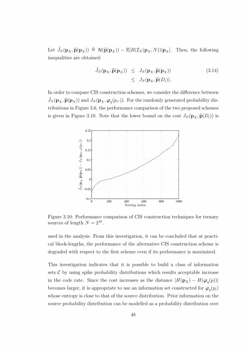
Let JN(pX , p(pX)) , H(p(pX)) − E[R(IX(pX , N))|pX ]. Then, the following
inequalities are obtained:
JN(pX , p(pX)) ≤ JN(pX , p(pX)) (3.14)
≤ JN(pX , p(Di)).
In order to compare CIS construction schemes, we consider the difference between
JN(pX , p(pX)) and JN(pX ,ϕq(pi∗)). For the randomly generated probability dis-
tributions in Figure 3.6, the performance comparison of the two proposed schemes
is given in Figure 3.10. Note that the lower bound on the cost JN(pX , p(Di)) is
0 200 400 600 800 1000−0.1
−0.05
0
0.05
0.1
0.15
0.2
0.25
JN
(pX
,p(p
X))−
JN
(pX
,ϕ(p
i∗))
Sorting index
Figure 3.10: Performance comparison of CIS construction techniques for ternarysources of length N = 210.
used in the analysis. From this investigation, it can be concluded that at practi-
cal block-lengths, the performance of the alternative CIS construction scheme is
degraded with respect to the first scheme even if its performance is maximized.
This investigation indicates that it is possible to build a class of information
sets C by using spike probability distributions which results acceptable increase
in the code rate. Since the cost increases as the distance |H(pX) − H(ϕq(p))|
becomes larger, it is appropriate to use an information set constructed for ϕq(pi)
whose entropy is close to that of the source distribution. Prior information on the
source probability distribution can be modelled as a probability distribution over
48
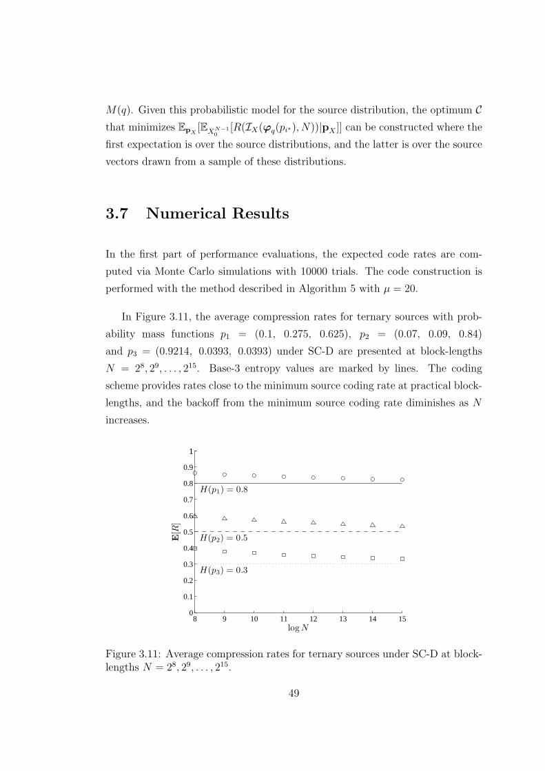
M(q). Given this probabilistic model for the source distribution, the optimum C
that minimizes EpX[EXN−1
0
[R(IX(ϕq(pi∗), N))|pX ]] can be constructed where the
first expectation is over the source distributions, and the latter is over the source
vectors drawn from a sample of these distributions.
3.7 Numerical Results
In the first part of performance evaluations, the expected code rates are com-
puted via Monte Carlo simulations with 10000 trials. The code construction is
performed with the method described in Algorithm 5 with µ = 20.
In Figure 3.11, the average compression rates for ternary sources with prob-
ability mass functions p1 = (0.1, 0.275, 0.625), p2 = (0.07, 0.09, 0.84)
and p3 = (0.9214, 0.0393, 0.0393) under SC-D are presented at block-lengths
N = 28, 29, . . . , 215. Base-3 entropy values are marked by lines. The coding
scheme provides rates close to the minimum source coding rate at practical block-
lengths, and the backoff from the minimum source coding rate diminishes as N
increases.
8 9 10 11 12 13 14 150
0.1
0.2
0.3
0.4
0.5
0.6
0.7
0.8
0.9
11
logN
E[R
]
H(p2) = 0.5
H(p1) = 0.8
H(p3) = 0.3
Figure 3.11: Average compression rates for ternary sources under SC-D at block-lengths N = 28, 29, . . . , 215.
49
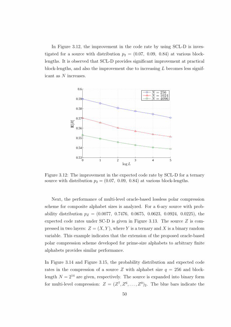
In Figure 3.12, the improvement in the code rate by using SCL-D is inves-
tigated for a source with distribution p2 = (0.07, 0.09, 0.84) at various block-
lengths. It is observed that SCL-D provides significant improvement at practical
block-lengths, and also the improvement due to increasing L becomes less signif-
icant as N increases.
0 1 2 3 4 50.53
0.54
0.55
0.56
0.57
0.58
0.59
0.6
logL
E[R
]
N = 256N = 1024N = 4096
Figure 3.12: The improvement in the expected code rate by SCL-D for a ternarysource with distribution p2 = (0.07, 0.09, 0.84) at various block-lengths.
Next, the performance of multi-level oracle-based lossless polar compression
scheme for composite alphabet sizes is analyzed. For a 6-ary source with prob-
ability distribution pZ = (0.0077, 0.7476, 0.0675, 0.0623, 0.0924, 0.0225), the
expected code rates under SC-D is given in Figure 3.13. The source Z is com-
pressed in two layers: Z = (X, Y ), where Y is a ternary and X is a binary random
variable. This example indicates that the extension of the proposed oracle-based
polar compression scheme developed for prime-size alphabets to arbitrary finite
alphabets provides similar performance.
In Figure 3.14 and Figure 3.15, the probability distribution and expected code
rates in the compression of a source Z with alphabet size q = 256 and block-
length N = 214 are given, respectively. The source is expanded into binary form
for multi-level compression: Z = (Z7, Z6, . . . , Z0)2. The blue bars indicate the
50
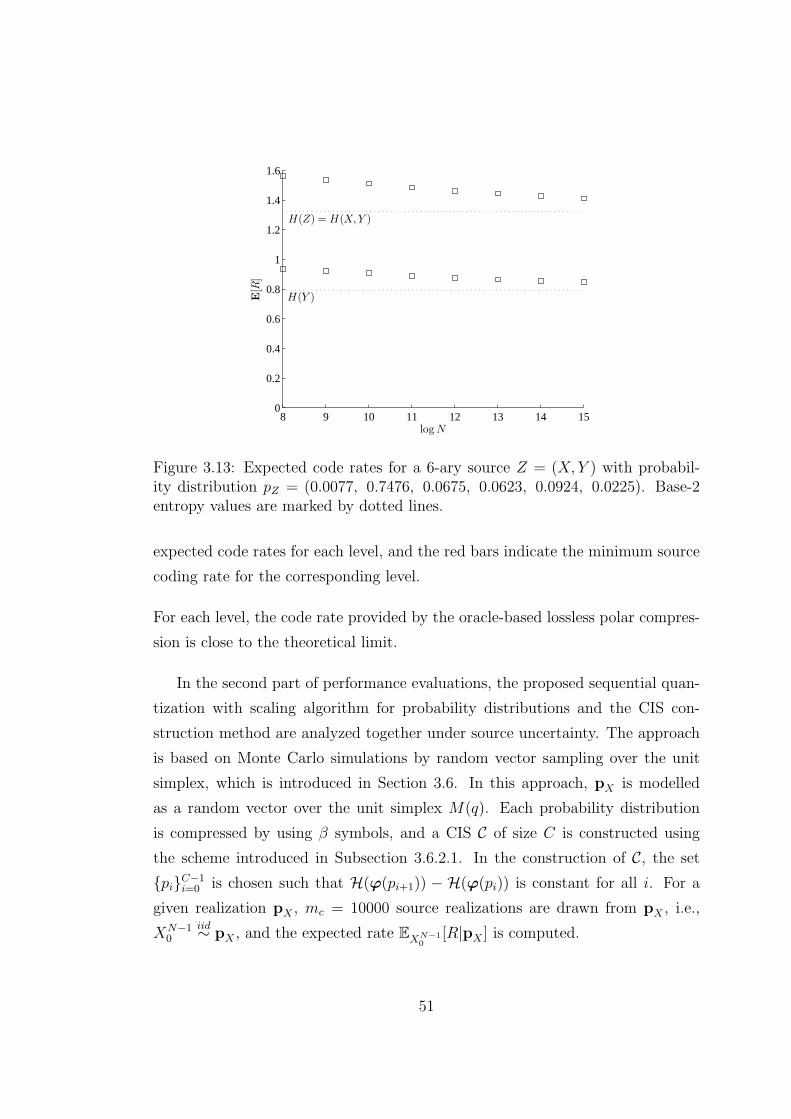
8 9 10 11 12 13 14 150
0.2
0.4
0.6
0.8
1
1.2
1.4
1.6
log N
E[R
]
H(Z) = H(X,Y )
H(Y )
Figure 3.13: Expected code rates for a 6-ary source Z = (X, Y ) with probabil-ity distribution pZ = (0.0077, 0.7476, 0.0675, 0.0623, 0.0924, 0.0225). Base-2entropy values are marked by dotted lines.
expected code rates for each level, and the red bars indicate the minimum source
coding rate for the corresponding level.
For each level, the code rate provided by the oracle-based lossless polar compres-
sion is close to the theoretical limit.
In the second part of performance evaluations, the proposed sequential quan-
tization with scaling algorithm for probability distributions and the CIS con-
struction method are analyzed together under source uncertainty. The approach
is based on Monte Carlo simulations by random vector sampling over the unit
simplex, which is introduced in Section 3.6. In this approach, pX is modelled
as a random vector over the unit simplex M(q). Each probability distribution
is compressed by using β symbols, and a CIS C of size C is constructed using
the scheme introduced in Subsection 3.6.2.1. In the construction of C, the set
{pi}C−1i=0 is chosen such that H(ϕ(pi+1)) − H(ϕ(pi)) is constant for all i. For a
given realization pX , mc = 10000 source realizations are drawn from pX , i.e.,
XN−10
iid∼ pX , and the expected rate EXN−1
0
[R|pX ] is computed.
51
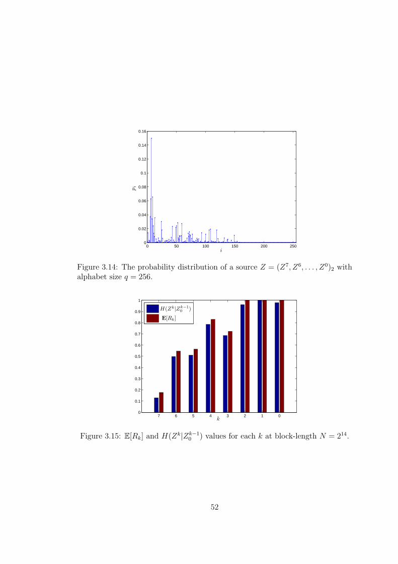
0 50 100 150 200 2500
0.02
0.04
0.06
0.08
0.1
0.12
0.14
0.16
i
pi
Figure 3.14: The probability distribution of a source Z = (Z7, Z6, . . . , Z0)2 withalphabet size q = 256.
7 6 5 4 3 2 1 00
0.1
0.2
0.3
0.4
0.5
0.6
0.7
0.8
0.9
1
k
H(Zk|Zk−1
0)
E[Rk]
Figure 3.15: E[Rk] and H(Zk|Zk−10 ) values for each k at block-length N = 214.
52
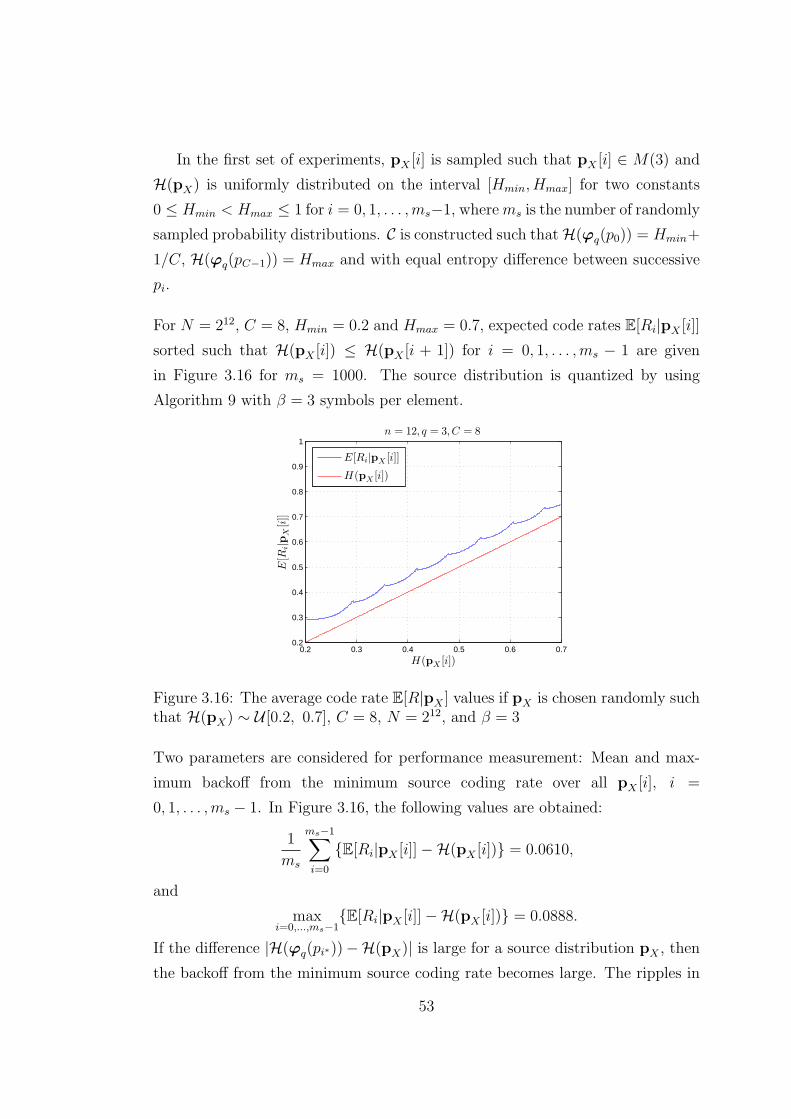
In the first set of experiments, pX [i] is sampled such that pX [i] ∈ M(3) and
H(pX) is uniformly distributed on the interval [Hmin, Hmax] for two constants
0 ≤ Hmin < Hmax ≤ 1 for i = 0, 1, . . . ,ms−1, wherems is the number of randomly
sampled probability distributions. C is constructed such thatH(ϕq(p0)) = Hmin+
1/C, H(ϕq(pC−1)) = Hmax and with equal entropy difference between successive
pi.
For N = 212, C = 8, Hmin = 0.2 and Hmax = 0.7, expected code rates E[Ri|pX [i]]
sorted such that H(pX [i]) ≤ H(pX [i + 1]) for i = 0, 1, . . . ,ms − 1 are given
in Figure 3.16 for ms = 1000. The source distribution is quantized by using
Algorithm 9 with β = 3 symbols per element.
0.2 0.3 0.4 0.5 0.6 0.70.2
0.3
0.4
0.5
0.6
0.7
0.8
0.9
1n = 12, q = 3, C = 8
H(pX
[i])
E[R
i|p
X[i]]
E[Ri|pX[i]]
H(pX
[i])
Figure 3.16: The average code rate E[R|pX ] values if pX is chosen randomly suchthat H(pX) ∼ U [0.2, 0.7], C = 8, N = 212, and β = 3
Two parameters are considered for performance measurement: Mean and max-
imum backoff from the minimum source coding rate over all pX [i], i =
0, 1, . . . ,ms − 1. In Figure 3.16, the following values are obtained:
1
ms
ms−1∑
i=0
{E[Ri|pX [i]]−H(pX [i])} = 0.0610,
and
maxi=0,...,ms−1
{E[Ri|pX [i]]−H(pX [i])} = 0.0888.
If the difference |H(ϕq(pi∗))−H(pX)| is large for a source distribution pX , then
the backoff from the minimum source coding rate becomes large. The ripples in
53
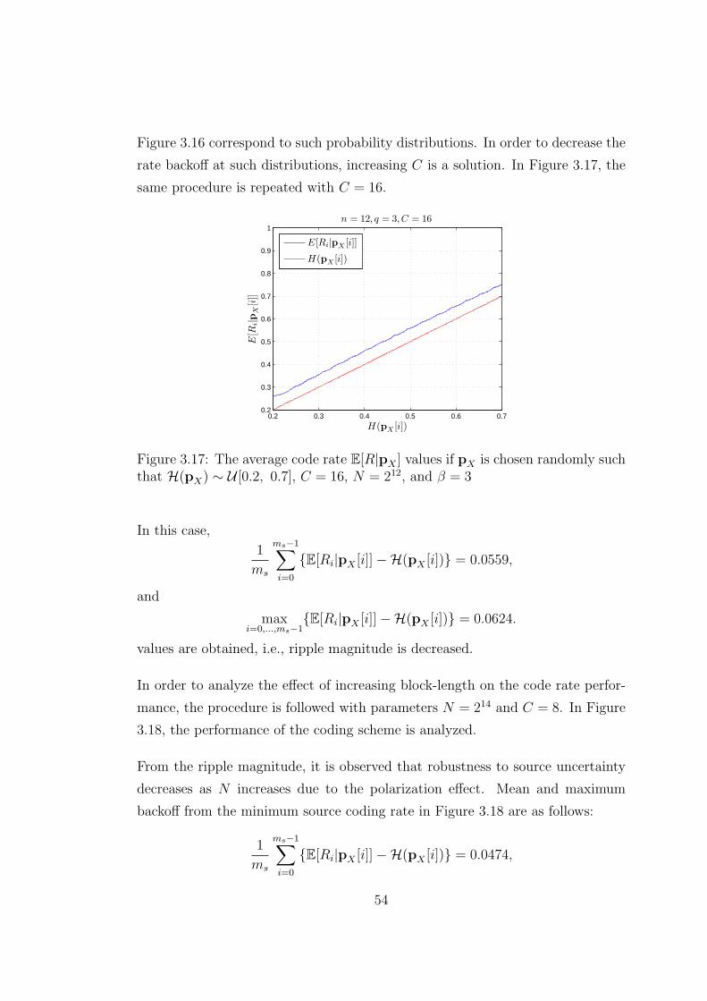
Figure 3.16 correspond to such probability distributions. In order to decrease the
rate backoff at such distributions, increasing C is a solution. In Figure 3.17, the
same procedure is repeated with C = 16.
0.2 0.3 0.4 0.5 0.6 0.70.2
0.3
0.4
0.5
0.6
0.7
0.8
0.9
1n = 12, q = 3, C = 16
H(pX
[i])
E[R
i|p
X[i]]
E[Ri|pX[i]]
H(pX
[i])
Figure 3.17: The average code rate E[R|pX ] values if pX is chosen randomly suchthat H(pX) ∼ U [0.2, 0.7], C = 16, N = 212, and β = 3
In this case,
1
ms
ms−1∑
i=0
{E[Ri|pX [i]]−H(pX [i])} = 0.0559,
and
maxi=0,...,ms−1
{E[Ri|pX [i]]−H(pX [i])} = 0.0624.
values are obtained, i.e., ripple magnitude is decreased.
In order to analyze the effect of increasing block-length on the code rate perfor-
mance, the procedure is followed with parameters N = 214 and C = 8. In Figure
3.18, the performance of the coding scheme is analyzed.
From the ripple magnitude, it is observed that robustness to source uncertainty
decreases as N increases due to the polarization effect. Mean and maximum
backoff from the minimum source coding rate in Figure 3.18 are as follows:
1
ms
ms−1∑
i=0
{E[Ri|pX [i]]−H(pX [i])} = 0.0474,
54
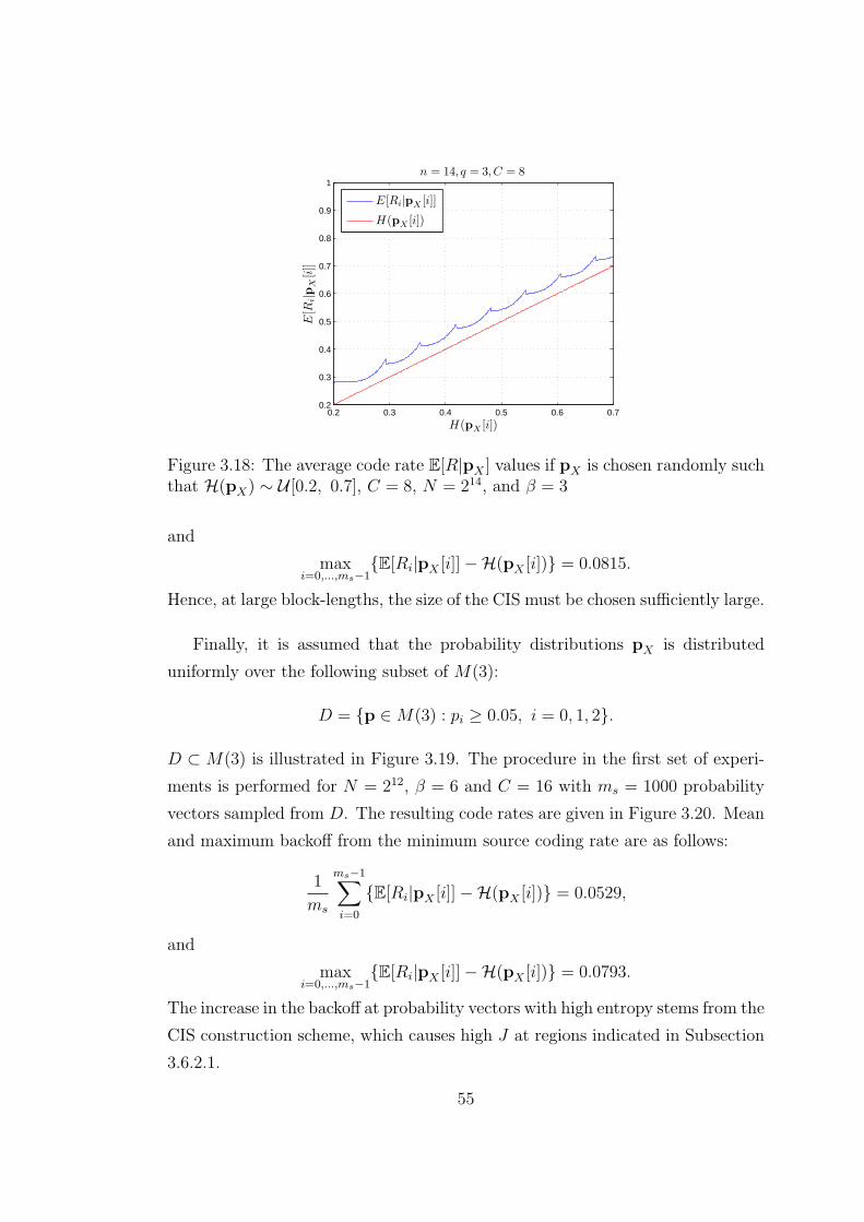
0.2 0.3 0.4 0.5 0.6 0.70.2
0.3
0.4
0.5
0.6
0.7
0.8
0.9
1n = 14, q = 3, C = 8
H(pX
[i])
E[R
i|p
X[i]]
E[Ri|pX[i]]
H(pX
[i])
Figure 3.18: The average code rate E[R|pX ] values if pX is chosen randomly suchthat H(pX) ∼ U [0.2, 0.7], C = 8, N = 214, and β = 3
and
maxi=0,...,ms−1
{E[Ri|pX [i]]−H(pX [i])} = 0.0815.
Hence, at large block-lengths, the size of the CIS must be chosen sufficiently large.
Finally, it is assumed that the probability distributions pX is distributed
uniformly over the following subset of M(3):
D = {p ∈ M(3) : pi ≥ 0.05, i = 0, 1, 2}.
D ⊂ M(3) is illustrated in Figure 3.19. The procedure in the first set of experi-
ments is performed for N = 212, β = 6 and C = 16 with ms = 1000 probability
vectors sampled from D. The resulting code rates are given in Figure 3.20. Mean
and maximum backoff from the minimum source coding rate are as follows:
1
ms
ms−1∑
i=0
{E[Ri|pX [i]]−H(pX [i])} = 0.0529,
and
maxi=0,...,ms−1
{E[Ri|pX [i]]−H(pX [i])} = 0.0793.
The increase in the backoff at probability vectors with high entropy stems from the
CIS construction scheme, which causes high J at regions indicated in Subsection
3.6.2.1.
55
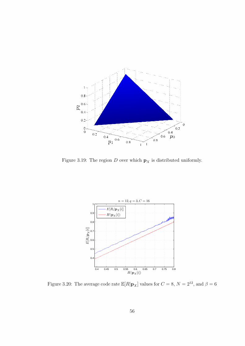
Figure 3.19: The region D over which pX is distributed uniformly.
0.4 0.45 0.5 0.55 0.6 0.65 0.7 0.75 0.8
0.4
0.5
0.6
0.7
0.8
0.9
1n = 12, q = 3, C = 16
H(pX
[i])
E[R
i|p
X[i]]
E[Ri|pX[i]]
H(pX
[i])
Figure 3.20: The average code rate E[R|pX ] values for C = 8, N = 212, and β = 6
56
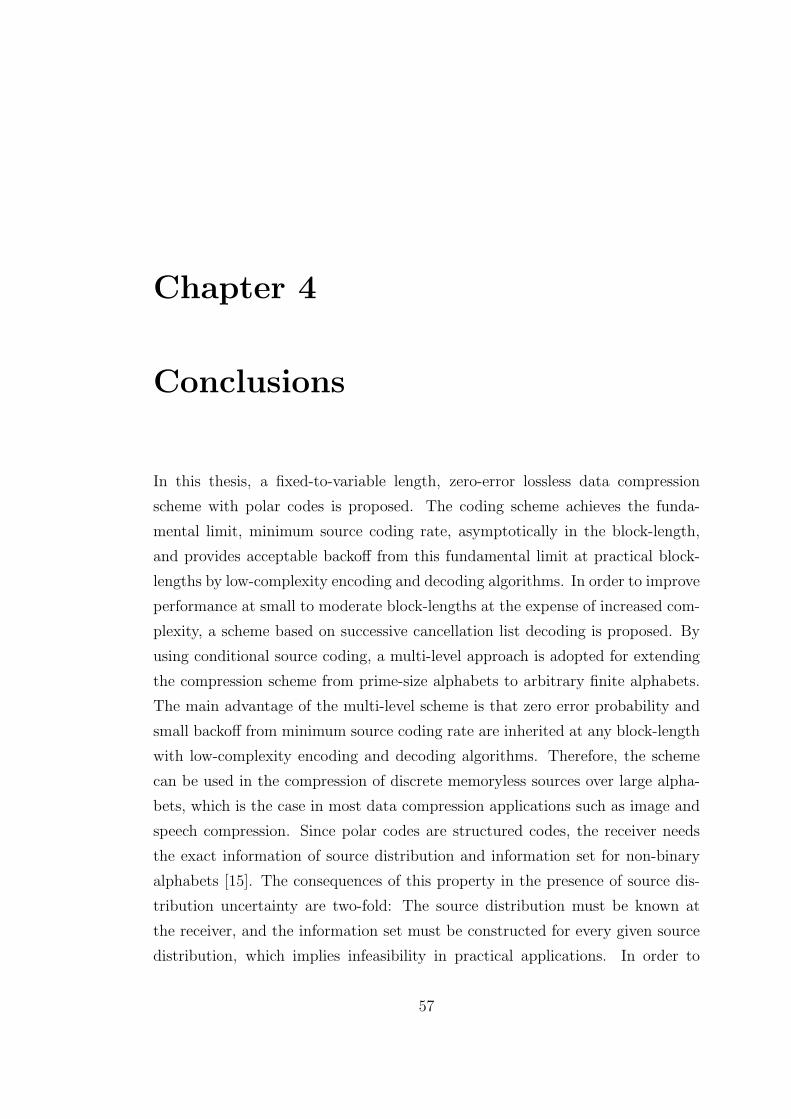
Chapter 4
Conclusions
In this thesis, a fixed-to-variable length, zero-error lossless data compression
scheme with polar codes is proposed. The coding scheme achieves the funda-
mental limit, minimum source coding rate, asymptotically in the block-length,
and provides acceptable backoff from this fundamental limit at practical block-
lengths by low-complexity encoding and decoding algorithms. In order to improve
performance at small to moderate block-lengths at the expense of increased com-
plexity, a scheme based on successive cancellation list decoding is proposed. By
using conditional source coding, a multi-level approach is adopted for extending
the compression scheme from prime-size alphabets to arbitrary finite alphabets.
The main advantage of the multi-level scheme is that zero error probability and
small backoff from minimum source coding rate are inherited at any block-length
with low-complexity encoding and decoding algorithms. Therefore, the scheme
can be used in the compression of discrete memoryless sources over large alpha-
bets, which is the case in most data compression applications such as image and
speech compression. Since polar codes are structured codes, the receiver needs
the exact information of source distribution and information set for non-binary
alphabets [15]. The consequences of this property in the presence of source dis-
tribution uncertainty are two-fold: The source distribution must be known at
the receiver, and the information set must be constructed for every given source
distribution, which implies infeasibility in practical applications. In order to
57
solve these problems, a probability mass function quantization algorithm and a
scheme for constructing and using pre-built information sets are proposed. For
analyzing the robustness of the proposed schemes to source uncertainty, a Monte
Carlo-based method is developed.
In [28] and [29], bounds are introduced for lossless data compression rate at
finite block-lengths. For performance evaluation, the performance of the proposed
compression scheme at non-asymptotic regime can be compared to these bounds.
As a first application of the proposed zero-error compression framework, DCT-
based JPEG image compression using polar compression is proposed. For im-
proved performance, polar JPEG compression schemes with Burrows-Wheeler
Transform [30, 31] and second generation wavelets [32] can be implemented. In
these schemes, a mixed multi-level approach with lossless and lossy polar com-
pression methods can be utilized for performance improvement. Together with a
method for exploiting the memory information, the proposed compression method
can be used in the compression of any signal efficiently.
58
Bibliography
[1] E. Arıkan, “Channel polarization: A method for constructing capacity-
achieving codes for symmetric binary-input memoryless channels,” IEEE
Transactions on Information Theory, vol. 55, no. 7, pp. 3051–3073, 2009.
[2] D. Slepian and J. K. Wolf, “Noiseless coding of correlated information
sources,” IEEE Transactions on Information Theory, vol. 19, no. 4, pp. 471–
480, 1973.
[3] R. M. Gray, “Conditional rate-distortion theory,” Technical report, No. 6502-
2, Information Systems Laboratory, Stanford Electronics Laboratories, 1972.
[4] S. C. Draper and E. Martinian, “Compound conditional source coding,
slepian-wolf list decoding, and applications to media coding,” in IEEE In-
ternational Symposium on Information Theory, ISIT 2007, pp. 1511–1515,
2007.
[5] I. Csiszar and J. Korner, Information Theory: Coding Theorems for Discrete
Memoryless Systems. Orlando, FL, USA: Academic Press, Inc., 1982.
[6] N. Hussami, S. B. Korada, and R. Urbanke, “Performance of polar codes for
channel and source coding,” in IEEE International Symposium on Informa-
tion Theory, ISIT 2009, pp. 1488–1492, 2009.
[7] S. B. Korada, “Polar codes for channel and source coding,” Ph.D. disser-
tation, Computer, Communication and Information Sciences, EPFL, Lau-
sanne, Switzerland, 2009.
59
[8] E. Arıkan, “Source polarization,” in IEEE International Symposium on In-
formation Theory Proceedings, ISIT 2010, pp. 899–903, 2010.
[9] H. S. Cronie and S. B. Korada, “Lossless source coding with polar codes,”
in IEEE International Symposium on Information Theory Proceedings, ISIT
2010, pp. 904–908, 2010.
[10] G. Caire, S. Shamai, and S. Verdu, Noiseless data compression with low-
density parity-check codes. Advances in network information theory, Piyush
Gupta, Gerhard Kramer, and Adriaan J. van Wijnggaardenl (Eds), Volume
66, DIMACS Series in Discrete Mathematics and Theoretical Computer Sci-
ence, 09 2004.
[11] E. Sasoglu, E. Telatar, and E. Arıkan, “Polarization for arbitrary discrete
memoryless channels,” CoRR, vol. abs/0908.0302, 2009.
[12] I. Dumer and K. Shabunov, “Soft-decision decoding of reed-muller codes:
recursive lists,” IEEE Transactions on Information Theory, vol. 52, no. 3,
pp. 1260–1266, 2006.
[13] R. Mori and T. Tanaka, “Performance and construction of polar codes on
symmetric binary-input memoryless channels,” in IEEE International Sym-
posium on Information Theory, ISIT 2009, pp. 1496–1500, 2009.
[14] I. Tal and A. Vardy, “How to construct polar codes,” CoRR,
vol. abs/1105.6164, 2011.
[15] E. Abbe, “Universal polar coding and sparse recovery,” CoRR,
vol. abs/1012.0367, 2010.
[16] E. Sasoglu, “Polar coding theorems for discrete systems,” Ph.D. disserta-
tion, Computer, Communication and Information Sciences, EPFL, Lau-
sanne, Switzerland, 2011.
[17] I. Tal and A. Vardy, “List decoding of polar codes,” CoRR,
vol. abs/1206.0050, 2012.
60
[18] I. Tal, A. Sharov, and A. Vardy, “Constructing polar codes for non-binary al-
phabets and macs,” in IEEE International Symposium on Information The-
ory Proceedings, ISIT 2012, pp. 2132–2136, 2012.
[19] R. Pedarsani, S. H. Hassani, I. Tal, and I. E. Telatar, “On the construction
of polar codes,” in IEEE International Symposium on Information Theory
Proceedings, ISIT 2011, pp. 11–15, 2011.
[20] M. T. Heath, Scientific Computing: An Introductory Survey. McGraw-Hill
Higher Education, 2nd ed., 2002.
[21] S. Caycı and O. Arıkan, “Lossless polar compression of q-ary sources,” in
IEEE International Symposium on Information Theory Proceedings, ISIT
2013, 2013.
[22] M. Feder and N. Merhav, “Relations between entropy and error probability,”
IEEE Transactions on Information Theory, vol. 40, no. 1, pp. 259–266, 1994.
[23] R. M. Gray, “Toeplitz and circulant matrices: A review,” Foundations and
Trends in Communications and Information Theory, vol. 2, no. 3, 2005.
[24] B. A. Frigyik, A. Kapila, and M. R. Gupta, “Introduction to the dirichlet
distribution and related processes,” Department of Electrical Engineering,
University of Washington, UWEETR-2010-0006, 2010.
[25] S. Onn and I. Weissman, “Generating uniform random vectors over a simplex
with implications to the volume of a certain polytope and to multivariate
extremes,” Annals of Operations Research, vol. 189, no. 1, pp. 331–342, 2011.
[26] D. P. Kroese, T. Taimre, and Z. I. Botev, Handbook of Monte Carlo Methods,
vol. 706. John Wiley & Sons, 2011.
[27] R. Tempo, G. Calafiore, and F. Dabbene, Randomized Algorithms for Anal-
ysis and Control of Uncertain Systems with Applications. Springer, 2nd ed.,
2013.
[28] W. Szpankowski and S. Verdu, “Minimum expected length of fixed-to-
variable lossless compression without prefix constraints,” IEEE Transactions
on Information Theory, vol. 57, no. 7, pp. 4017–4025, 2011.
61
[29] S. Verdu and I. Kontoyiannis, “Lossless data compression rate: Asymptotics
and non-asymptotics,” in 46th Annual Conference on Information Sciences
and Systems (CISS), pp. 1–6, IEEE, 2012.
[30] M. Burrows and D. J. Wheeler, “A block-sorting lossless data compression
algorithm,” tech. rep., Digital Equipment Corporation, 1994.
[31] M. Effros, K. Visweswariah, S. R. Kulkarni, and S. Verdu, “Universal lossless
source coding with the burrows wheeler transform,” IEEE Transactions on
Information Theory, vol. 48, no. 5, pp. 1061–1081, 2002.
[32] W. Sweldens, “The lifting scheme: A construction of second generation
wavelets,” SIAM Journal on Mathematical Analysis, vol. 29, no. 2, pp. 511–
546, 1998.
62