Lossless Data Compression - CCSDS.org · CCSDS REPORT CONCERNING LOSSLESS DATA COMPRESSION CCSDS...

Report Concerning Space Data System Standards

GREEN BOOK

LOSSLESS DATA COMPRESSION

INFORMATIONAL REPORT

CCSDS 120.0-G-3

April 2013

Report Concerning Space Data System Standards

LOSSLESS DATA COMPRESSION

INFORMATIONAL REPORT

CCSDS 120.0-G-3

GREEN BOOK April 2013

CCSDS REPORT CONCERNING LOSSLESS DATA COMPRESSION

CCSDS 120.0-G-3 Page i April 2013

AUTHORITY

Issue: Informational Report, Issue 3

Date: April 2013

Location: Washington, DC, USA

This document has been approved for publication by the Management Council of the Consultative Committee for Space Data Systems (CCSDS) and reflects the consensus of technical panel experts from CCSDS Member Agencies. The procedure for review and authorization of CCSDS Reports is detailed in Organization and Processes for the Consultative Committee for Space Data Systems (CCSDS A02.1-Y-3).

This document is published and maintained by:

CCSDS Secretariat Space Communications and Navigation Office, 7L70 Space Operations Mission Directorate NASA Headquarters Washington, DC 20546-0001, USA


CCSDS 120.0-G-3 Page ii April 2013

FOREWORD

This document is a CCSDS Report which contains background and explanatory material to support the CCSDS Recommendation, Lossless Data Compression (reference [1]).

Through the process of normal evolution, it is expected that expansion, deletion, or modification of this document may occur. This Report is therefore subject to CCSDS document management and change control procedures, which are defined in Organization and Processes for the Consultative Committee for Space Data Systems (CCSDS A02.1-Y-3). Current versions of CCSDS documents are maintained at the CCSDS Web site:

http://www.ccsds.org/

Questions relating to the contents or status of this document should be addressed to the CCSDS Secretariat at the address indicated on page i.


CCSDS 120.0-G-3 Page iii April 2013

At time of publication, the active Member and Observer Agencies of the CCSDS were:

Member Agencies

– Agenzia Spaziale Italiana (ASI)/Italy. – Canadian Space Agency (CSA)/Canada. – Centre National d’Etudes Spatiales (CNES)/France. – China National Space Administration (CNSA)/People’s Republic of China. – Deutsches Zentrum für Luft- und Raumfahrt e.V. (DLR)/Germany. – European Space Agency (ESA)/Europe. – Federal Space Agency (FSA)/Russian Federation. – Instituto Nacional de Pesquisas Espaciais (INPE)/Brazil. – Japan Aerospace Exploration Agency (JAXA)/Japan. – National Aeronautics and Space Administration (NASA)/USA. – UK Space Agency/United Kingdom.

Observer Agencies

– Austrian Space Agency (ASA)/Austria. – Belgian Federal Science Policy Office (BFSPO)/Belgium. – Central Research Institute of Machine Building (TsNIIMash)/Russian Federation. – China Satellite Launch and Tracking Control General, Beijing Institute of Tracking

and Telecommunications Technology (CLTC/BITTT)/China. – Chinese Academy of Sciences (CAS)/China. – Chinese Academy of Space Technology (CAST)/China. – Commonwealth Scientific and Industrial Research Organization (CSIRO)/Australia. – CSIR Satellite Applications Centre (CSIR)/Republic of South Africa. – Danish National Space Center (DNSC)/Denmark. – Departamento de Ciência e Tecnologia Aeroespacial (DCTA)/Brazil. – European Organization for the Exploitation of Meteorological Satellites

(EUMETSAT)/Europe. – European Telecommunications Satellite Organization (EUTELSAT)/Europe. – Geo-Informatics and Space Technology Development Agency (GISTDA)/Thailand. – Hellenic National Space Committee (HNSC)/Greece. – Indian Space Research Organization (ISRO)/India. – Institute of Space Research (IKI)/Russian Federation. – KFKI Research Institute for Particle & Nuclear Physics (KFKI)/Hungary. – Korea Aerospace Research Institute (KARI)/Korea. – Ministry of Communications (MOC)/Israel. – National Institute of Information and Communications Technology (NICT)/Japan. – National Oceanic and Atmospheric Administration (NOAA)/USA. – National Space Agency of the Republic of Kazakhstan (NSARK)/Kazakhstan. – National Space Organization (NSPO)/Chinese Taipei. – Naval Center for Space Technology (NCST)/USA. – Scientific and Technological Research Council of Turkey (TUBITAK)/Turkey. – Space and Upper Atmosphere Research Commission (SUPARCO)/Pakistan. – Swedish Space Corporation (SSC)/Sweden. – United States Geological Survey (USGS)/USA.


CCSDS 120.0-G-3 Page iv April 2013

DOCUMENT CONTROL

Document Title Date Status

CCSDS 120.0-G-1

Lossless Data Compression, Informational Report, Issue 1

May 1997 Original issue, superseded

CCSDS 120.0-G-2


December 2006

Issue 2, superseded

CCSDS 120.0-G-3


April 2013 Current issue: – updates material

affected by revision of the Lossless Data Compression Blue Book


CCSDS 120.0-G-3 Page v April 2013

CONTENTS

Section Page

1 INTRODUCTION .......................................................................................................... 1-1 1.1 PURPOSE ............................................................................................................... 1-1 1.2 SCOPE .................................................................................................................... 1-1 1.3 DEFINITIONS ........................................................................................................ 1-1 1.4 REFERENCES ....................................................................................................... 1-1

2 OVERVIEW ................................................................................................................... 2-1 3 ALGORITHM ................................................................................................................ 3-2

3.1 GENERAL .............................................................................................................. 3-2 3.2 ENTROPY CODER ............................................................................................... 3-4 3.3 THE PREPROCESSOR ......................................................................................... 3-8

4 SYSTEMS ISSUES ........................................................................................................ 4-1

4.1 INTRODUCTION .................................................................................................. 4-1 4.2 SENSOR CHARACTERISTICS ............................................................................ 4-1 4.3 ERROR PROPAGATION ...................................................................................... 4-2 4.4 DATA PACKETIZATION AND COMPRESSION PERFORMANCE ............... 4-2 4.5 BUFFER REQUIREMENT .................................................................................... 4-3

5 IMPLEMENTATION ................................................................................................... 5-1

5.1 OVERVIEW ........................................................................................................... 5-1 5.2 SPACE SEGMENT ................................................................................................ 5-1 5.3 GROUND SEGMENT ........................................................................................... 5-2 5.4 DECODING ............................................................................................................ 5-3

6 PERFORMANCE .......................................................................................................... 6-1

6.1 MEASURE ............................................................................................................. 6-1 6.2 EXAMPLES ........................................................................................................... 6-1

ANNEX A VERIFYING CCSDS LOSSLESS DATA COMPRESSION

ENCODER IMPLEMENTATION .............................................................. A-1 ANNEX B ACRONYMS AND ABBREVIATIONS .......................................................B-1


CCSDS 120.0-G-3 Page vi April 2013

CONTENTS (continued)

Figure Page

2-1 Packet Telemetry Data System ..................................................................................... 2-1 3-1 The Encoder Architecture ............................................................................................. 3-3 3-2 Performance Curve for Various k ................................................................................. 3-5 3-3 Effective Performance Curve ........................................................................................ 3-5 3-4 Example of All-Zero Blocks ......................................................................................... 3-7 3-5 Block Diagram of Unit-Delay Predictive Preprocessor and Postprocessor.................. 3-8 3-6 Two Dimensional Predictor of an Image

Where x(i, j) Is the Sample to Be Predicted ................................................................. 3-9 3-7a Relative Position of Sample Value xi and Predictor Value x̂i ................................... 3-11 3-7b Typical Probability Distribution Function (pdf) of Δi for Imaging Data .................. 3-11 4-1 Push-Broom Scanning Scheme ..................................................................................... 4-1 4-2 Probability of Buffer Overflow..................................................................................... 4-4 5-1 The Space Segment ....................................................................................................... 5-1 5-2 Ground Segment ........................................................................................................... 5-2 5-3 Decoder Block Diagram ............................................................................................... 5-3 6-1 Landsat-4 Image ........................................................................................................... 6-2 6-2a An HSI Data Cube ........................................................................................................ 6-3 6-2b A VNIR Spatial-Spectral Plane .................................................................................... 6-3 6-2c A VNIR Spatial Plane ................................................................................................... 6-3 6-3 Heat Capacity Mapping Radiometer Image ................................................................. 6-4 6-4 Wide Field Planetary Camera Image ............................................................................ 6-5 6-5 Soft X-Ray Telescope Solar Image .............................................................................. 6-7 6-6 Goddard High Resolution Spectrometer ....................................................................... 6-8 6-7 Acousto-Optical Spectrometer Waveform .................................................................... 6-9 6-8 GRS Waveform ........................................................................................................... 6-10 6-9 Compression Results on GRS Data ............................................................................ 6-10

Table

3-1 Zero-Block Fundamental Sequence Codewords as a Function of the Number of Consecutive All-Zeros Blocks ......................................................... 3-6

5-1 Decoding Logic for the Second-Extension Option ....................................................... 5-4 6-1 Summary of Data Compression Performance for Different Scientific Data Sets ............ 6-2 6-2 Compression Ratio (CR) at Different Threshold Values .............................................. 6-6 6-3 Compression Ratio vs. Packet Size .............................................................................. 6-6 6-4 Compression Ratio for GHRS ...................................................................................... 6-8 6-5 SWAS Compression Result .......................................................................................... 6-9


CCSDS 120.0-G-3 Page 1-1 April 2013

1 INTRODUCTION

1.1 PURPOSE

This report presents a summary of the key operational concepts and rationale which underlie the requirements for the CCSDS Recommended Standard, Lossless Data Compression (reference [1]). Supporting performance information along with illustrations are also included. This report provides a broad tutorial overview of the CCSDS Lossless Data Compression algorithm and is aimed at helping first-time readers to understand the Recommended Standard.

1.2 SCOPE

This document provides supporting and descriptive material only: it is not part of the Recommended Standard. In the event of any conflict between the Lossless Data Compression Recommended Standard and the material presented herein, the Recommended Standard shall prevail.

1.3 DEFINITIONS

Channel Access Data Unit (CADU): A data unit consisting of the Attached Synchronization Marker (ASM) and either a CCSDS Version-2 (AOS) Transfer Frame or a Version-2 Transfer Frame to which a block of error-correcting Reed-Solomon check symbols has been appended. Coded Virtual Channel Data Unit (CVCDU): (deprecated) A Version-2 Transfer Frame to which a block of error-correcting Reed-Solomon check symbols has been appended. Virtual Channel Data Unit (VCDU): (deprecated) A Version-2 Transfer Frame.

1.4 REFERENCES

[1] Lossless Data Compression. Recommendation for Space Data System Standards, CCSDS 121.0-B-2. Blue Book. Issue 2. Washington, D.C.: CCSDS, May 2012.

[2] Organization and Processes for the Consultative Committee for Space Data Systems. CCSDS A02.1-Y-3. Yellow Book. Issue 3. Washington, D.C.: CCSDS, July 2011.

[3] Space Packet Protocol. Recommendation for Space Data System Standards, CCSDS 133.0-B-1. Blue Book. Issue 1. Washington, D.C.: CCSDS, September 2003.

[4] AOS Space Data Link Protocol. Recommendation for Space Data System Standards, CCSDS 732.0-B-2. Blue Book. Issue 2. Washington, D.C.: CCSDS, July 2006.



[5] Pen-Shu Yeh and Warner H. Miller. Application Guide for Universal Source Coding for Space. NASA Technical Paper 3441. Washington, DC: NASA, December 1993.

[6] Robert F. Rice, Pen-Shu Yeh, and Warner H. Miller. “Algorithms for High Speed Universal Noiseless Coding.” In Proceedings of AIAA Computing in Aerospace, IX (October 19-21, 1993, San Diego, CA). Reston, Virginia: AIAA, 1993.

[7] TM Synchronization and Channel Coding. Recommendation for Space Data System Standards, CCSDS 131.0-B-2. Blue Book. Issue 2. Washington, D.C.: CCSDS, August 2011.

[8] Pen-Shu Yeh, Robert Rice, and Warner Miller. On the Optimality of Code Options for a Universal Noiseless Coder. NASA/JPL Publication 91-2. Pasadena, California: JPL, February 15, 1991.

[9] Pen-Shu Yeh and Warner H. Miller. “A Real Time Lossless Data Compression Technology for Remote-Sensing and Other Applications.” In Proceeding of IEEE International Symposium on Circuits and Systems, 1995. ISCAS ’95 (30 Apr-3 May 1995, Seattle, Washington), Vol. 2:1098–1101. New York: IEEE, 1995.

[10] Masud Mansuripur. Introduction to Information Theory. Englewood Cliffs, N.J.: Prentice Hall, 1987.

[11] Lossless Multispectral & Hyperspectral Image Compression. Recommendation for Space Data System Standards, CCSDS 123.0-B-1. Blue Book. Issue 1. Washington, D.C.: CCSDS, May 2012.



2 OVERVIEW

Lossless data compression has been suggested for many space science exploration mission applications either to increase the science return or to reduce the requirement for on-board memory, station contact time, and data archival volume. A Lossless compression technique guarantees full reconstruction of the original data without incurring any distortion in the process.

The Lossless Data Compression technique recommended preserves the source data accuracy by removing redundancy from the application source data. In the decompression processes the original source data is reconstructed from the compressed data by restoring the removed redundancy. The reconstructed data is an exact replica of the original source data. The quantity of redundancy removed from the source data is variable and is highly dependent on the source data statistics, which are often non-stationary.

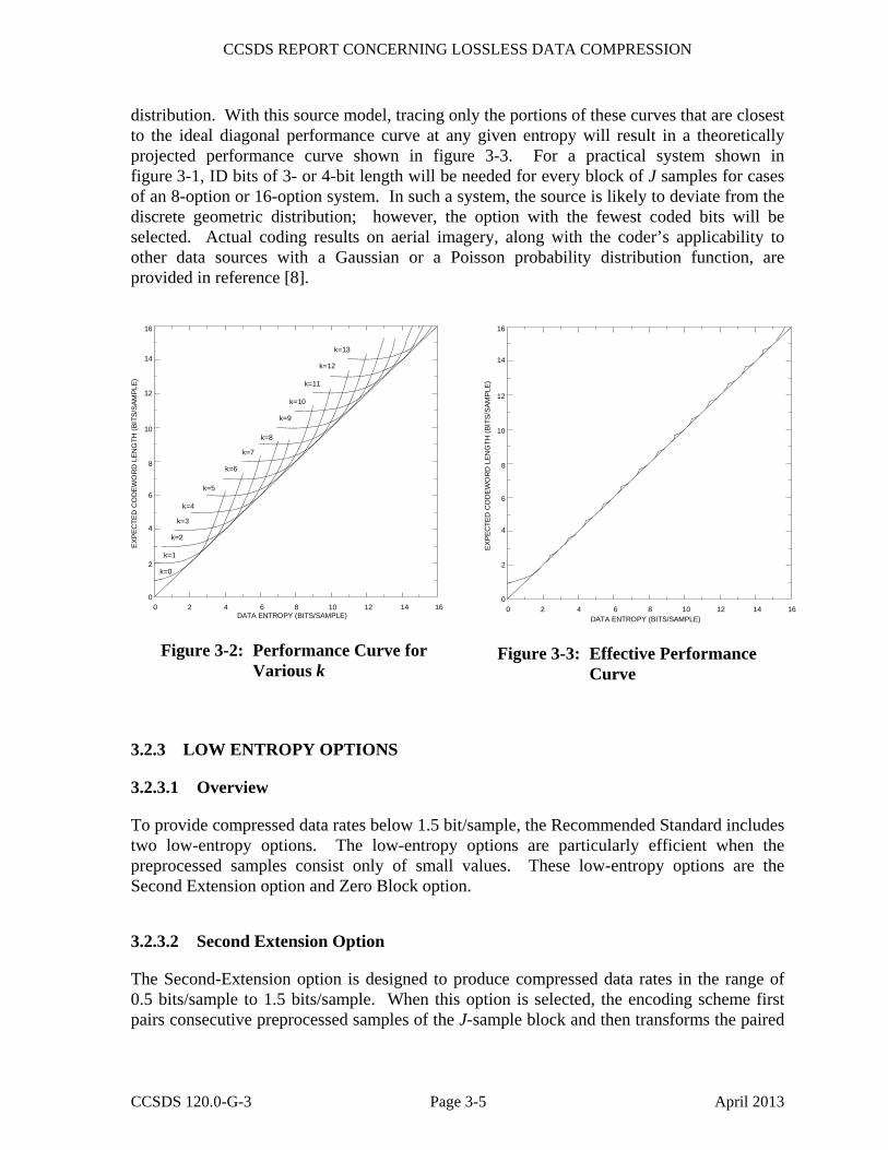
The Lossless Data Compression algorithm can be applied at the application data source or performed as a function of the on-board data system (see figure 2-1). The performance of the data compression algorithm is independent of where it is applied. However, if the data compression algorithm is part of the on-board data system, the on-board data system will, in general, have to capture the data in a buffer. In both cases, it may be necessary to rearrange the data into appropriate sequence before applying the data compression algorithm. The purpose of rearranging data is to improve the compression ratio.

After compression has been performed, the resulting variable-length data structure is then packetized as specified in reference [3]. The packets containing compressed data should be transported through a space-to-ground communication link from the source on-board a space vehicle to a data sink on the ground using a packet data system as shown in figure 2-1.

ApplicationData

Source

On-BoardData

System

Space-to-GroundChannel

GroundData

SystemData Sink

dnuorGdraoBnO

Figure 2-1: Packet Telemetry Data System

The essential purpose of the packet telemetry system is to permit the application processes on- board to create units of data called packets. These packets are then transmitted over the space-to-ground communication channel in a way that enables the ground system to recover the data with high reliability. The contents of the packets are then extracted and their data units are provided to the ground sink in sequence to be decompressed.

This document provides a top-level description of the Rice algorithm architecture, which is the basis for the compression technique (see reference [6]). It then addresses systems issues important for on-board implementation. The latter part of the document provides case-study examples drawn from a broad spectrum of science instruments (see reference [5]). Reference [9] also provides Lossless data compression results obtained from three different algorithms obtained from five data sets.



3 ALGORITHM

3.1 GENERAL

Implementation of a data-compression technique on a spacecraft will benefit from the following considerations:

a) the ability of the algorithm to adapt to changes in data statistics to maximize performance;

b) the requirements to minimize the number of processing steps and reduce memory and power usage;

c) the ability of the algorithm to operate in one pass;

d) the ability of the algorithm to be interfaced with a packetized data system without requiring a-priori information re-establishing data statistics for every packet;

e) the ability to limit the effects of a channel error.

There are a few well-known Lossless compression techniques, including Huffman coding, arithmetic coding, Ziv-Lempel coding, and variants of each. After extensive study of the above criteria and performance comparison on a set of test images, the Rice algorithm was selected for the CCSDS Recommended Standard (see reference [9]).

The Rice algorithm uses a set of variable-length codes to achieve compression. Each code is nearly optimal for a particular geometrically distributed source. Variable-length codes, such as Huffman codes and the codes used by the Rice algorithm, compress data by assigning shorter codewords to symbols that are expected to occur with higher frequency, as illustrated in 3.2.1. By using several different codes and transmitting the code identifier, the Rice algorithm can adapt to many sources from low entropy (more compressible) to high entropy (less compressible). Because blocks of source samples are encoded independently, side information does not need to be carried across packet boundaries, and the performance of the algorithm is independent of packet size. For a discussion of the term entropy, the reader should consult an information theory textbook such as reference [10].

A block diagram of the Rice algorithm is shown in figure 3-1. It consists of a preprocessor to decorrelate data samples and subsequently map them into symbols suitable for the entropy coding stage. The input data to the preprocessor, x, is a J-sample block of n-bit samples:

x = x1, x2, . . . xJ.

The preprocessor transforms input data into blocks of preprocessed samples, δ, where:

δ = δ1, δ2, . . . δJ.

The Adaptive Encoder converts preprocessed samples, δ, into an encoded bit sequence y.



SelectedCode

Option

OptionNo Compression

Preprocessor

Option2nd Extension

OptionFS

Optionk = 1

OptionZero-Block

Optionk = 2

Adaptive Entropy Coder

y

ID

δ=δ1,δ2,...,δJx=x1,x2,...,xJ

Code OptionSelection

Figure 3-1: The Encoder Architecture

The entropy coding module consists of a collection of variable-length codes that can be applied to each block of J preprocessed samples. For each block, the coding option achieving the best compression is selected to encode the block. The encoded block is preceded by an ID bit pattern that identifies the coding option to the decoder. Because a new code option can be selected for each block, the Rice algorithm can adapt to changing source statistics. Thus shorter values of the block length parameter J allow faster adaptation to changing source statistics. However, the fraction of encoded bits used to indicate the coding option (the ‘overhead’ associated with code option identification) decreases for larger values of J.

The first issue of the Recommended Standard allowed J to take values {8, 16}. In practice, longer block lengths often offer improved overall compression effectiveness (because of reduced overhead). Motivated by this fact—especially when the Recommended Standard is used as the entropy coding option for multispectral or hyperspectral image compression as specified in reference [11]—issue 2 of the Recommended Standard expands the allowed values of J to {8, 16, 32, 64}.



3.2 ENTROPY CODER

3.2.1 FUNDAMENTAL SEQUENCE ENCODING

To see how a variable length code can achieve data compression, consider two methods of encoding sequences from an alphabet of four symbols:

Symbol Code 1 Code 2 (FS Code) s1 00 1 s2 01 01 s3 10 001 s4 11 0001

It should be noted that the Code 2 is the Fundamental Sequence (FS) code.

Under either code, encoded bit streams corresponding to symbol sequences are uniquely decodable. For Code 1, it is recognized that every two encoded bits correspond to a symbol. For the FS code it is recognized that each ‘1’ digit signals the end of a codeword, and the number of preceding zeros identifies which symbol was transmitted. This simple decoding procedure allows FS codewords to be decoded without the use of lookup tables.

The reason that the FS code can achieve compression is that when symbol s1 occurs very frequently, and symbols s3 and s4 are very rare, on average fewer than two encoded bits per symbol will be will transmitted, whereas Code 1 always requires two encoded bits per symbol. Longer FS codes achieve compression in a similar manner.

3.2.2 THE SPLIT-SAMPLE OPTIONS

Most of the options in the entropy coder are called ‘split-sample options’. The kth split-sample option takes a block of J preprocessed data samples, splits off the k least significant bits from each sample and encodes the remaining higher order bits with a simple FS codeword before appending the split bits to the encoded FS data stream. Each split-sample option in the Rice algorithm is designed to produce compressed data with a range of about 1 bit/sample (approximately k + 1.5 to k + 2.5 bits/sample); the code option yielding the fewest encoded bits will be chosen for each block by the option-select logic. This option selection process assures that the block will be coded with the best available code option on the same block of data, but this does not necessarily imply that the source entropy lies in that range. The actual source entropy value could be lower; the source statistics and the effectiveness of the preprocessing stage determine how closely entropy can be approached.

A theoretical expected codeword length of the split-sample coding scheme is shown in figure 3-2 for various values of k, where k=0 is the fundamental sequence option. These curves are obtained under the assumption that the source approaches a discrete geometric



distribution. With this source model, tracing only the portions of these curves that are closest to the ideal diagonal performance curve at any given entropy will result in a theoretically projected performance curve shown in figure 3-3. For a practical system shown in figure 3-1, ID bits of 3- or 4-bit length will be needed for every block of J samples for cases of an 8-option or 16-option system. In such a system, the source is likely to deviate from the discrete geometric distribution; however, the option with the fewest coded bits will be selected. Actual coding results on aerial imagery, along with the coder’s applicability to other data sources with a Gaussian or a Poisson probability distribution function, are provided in reference [8].

16

14

12

10

6

4

2

00 2 4 6 8 10 12 14 16

8

DATA ENTROPY (BITS/SAMPLE)

k=0

k=1

k=2

k=3

k=4

k=5

k=6

k=7

k=8

k=9

k=10

k=11

k=12

k=13

EXPE

CTE

D C

OD

EWO

RD

LEN

GTH

(BIT

S/SA

MPL

E)

Figure 3-2: Performance Curve for Various k

16

14

12

10

6

4

2

00 2 4 6 8 10 12 14 16

8

DATA ENTROPY (BITS/SAMPLE)

EXPE

CTE

D C

OD

EWO

RD

LEN

GTH

(BIT

S/SA

MPL

E)

Figure 3-3: Effective Performance Curve

3.2.3 LOW ENTROPY OPTIONS

3.2.3.1 Overview

To provide compressed data rates below 1.5 bit/sample, the Recommended Standard includes two low-entropy options. The low-entropy options are particularly efficient when the preprocessed samples consist only of small values. These low-entropy options are the Second Extension option and Zero Block option.

3.2.3.2 Second Extension Option

The Second-Extension option is designed to produce compressed data rates in the range of 0.5 bits/sample to 1.5 bits/sample. When this option is selected, the encoding scheme first pairs consecutive preprocessed samples of the J-sample block and then transforms the paired



samples into a new value that is coded with an FS codeword. The FS codeword for γ is transmitted, where:

γ = (δi + δi+1) (δi + δi+1+1)/2 + δi+1

3.2.3.3 Zero-Block Option

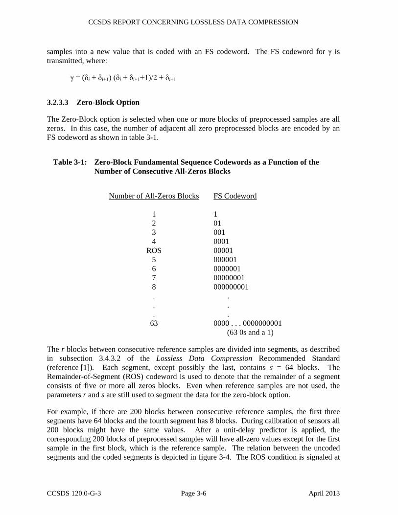
The Zero-Block option is selected when one or more blocks of preprocessed samples are all zeros. In this case, the number of adjacent all zero preprocessed blocks are encoded by an FS codeword as shown in table 3-1.

Table 3-1: Zero-Block Fundamental Sequence Codewords as a Function of the Number of Consecutive All-Zeros Blocks

Number of All-Zeros Blocks FS Codeword 1 1 2 01 3 001 4 0001

ROS 00001 5 000001 6 0000001 7 00000001 8 000000001 . . . . . .

63 0000 . . . 0000000001 (63 0s and a 1)

The r blocks between consecutive reference samples are divided into segments, as described in subsection 3.4.3.2 of the Lossless Data Compression Recommended Standard (reference [1]). Each segment, except possibly the last, contains s = 64 blocks. The Remainder-of-Segment (ROS) codeword is used to denote that the remainder of a segment consists of five or more all zeros blocks. Even when reference samples are not used, the parameters r and s are still used to segment the data for the zero-block option.

For example, if there are 200 blocks between consecutive reference samples, the first three segments have 64 blocks and the fourth segment has 8 blocks. During calibration of sensors all 200 blocks might have the same values. After a unit-delay predictor is applied, the corresponding 200 blocks of preprocessed samples will have all-zero values except for the first sample in the first block, which is the reference sample. The relation between the uncoded segments and the coded segments is depicted in figure 3-4. The ROS condition is signaled at



the end of each 64-block segment, and a new ID is issued at the beginning of each segment. It should be noted that the ROS condition also encodes the last eight all-zero blocks.

64 blocks 64 blocks 64 blocks8 blocks

200 blocksZe

ro-B

lock

ID

Ref

eren

ce

RO

S C

odew

ord

Zero

-Blo

ck ID

Zero

-Blo

ck ID

Zero

-Blo

ck ID

RO

S C

odew

ord

RO

S C

odew

ord

RO

S C

odew

ord

Coded

As:

tnemgestnemgestnemges

Figure 3-4: Example of All-Zero Blocks

3.2.4 NO-COMPRESSION OPTION

When none of the above options provides any data compression on a block, the no-compression option is selected. Under this option, the preprocessed block of data is transmitted without alteration except for a prefixed identifier.

3.2.5 OPTION SELECTION

For a block of samples, the entropy coder selects the option that minimizes the number of encoded bits. This includes the identifier bit sequence that specifies which code option was selected.

3.2.6 OPTION IDENTIFICATION

When the source dynamic range is small (i.e., for small values of resolution n), code options corresponding to larger values of k are not useful. For this reason, when n≤4, a user can choose to use the Restricted set of coding options (see table 5-1 of reference [1]), which limits the available coding options and thus reduces the number of bits used to identify the coding option. This reduces overhead and improves compression performance for certain low dynamic range data sources.



3.3 THE PREPROCESSOR

3.3.1 PREDICTOR

The role of the preprocessor is to transform the data into samples that can be more efficiently compressed by the entropy encoder. To ensure that compression is Lossless, the preprocessor must be reversible. It can be seen from the example in 3.2.1 that to achieve effective compression there needs to be a preprocessing stage that transforms the original data so that shorter codewords occur with higher probability than longer codewords. If there are several candidate preprocessing stages, it would be preferable to select the one that produces the shortest average codeword length.

In general a preprocessor that removes correlation between samples in the input data block will improve the performance of the entropy coder. In the following discussion, it is assumed that preprocessing is done by a predictor followed by a prediction error mapper. For some types of data, more sophisticated transform-based techniques can offer improved compression efficiency, at the expense of higher complexity.

The decorrelation function of the preprocessor can be implemented by a judicious choice of the predictor for an expected set of data samples. The selection of a predictor should take into account the expected data as well as possible variations in the background noise and the gain of the sensors acquiring the data. The predictor should be chosen to minimize the amount of noise resulting from sensor non-uniformity.

One of the simplest predictive coders is a linear first-order unit-delay predictor shown in figure 3-5a. The output, Δi, will be the difference between the input data symbol and the preceding data symbol.

UnitDelay

Mapperxi ∆i δi

x(i-1)

+

-

Demapper

UnitDelay

xi∆iδi

a) Preprocessor

b) Postprocessor

Figure 3-5: Block Diagram of Unit-Delay Predictive Preprocessor and Postprocessor

Several other predictors exist. In general, users may select any prediction scheme that best



decorrelates the input data stream. For example, consider an image with intensity values x(i, j) where i represents the scan line and j the pixel number within the scan (see figure 3-6). Possible predictor types include:

a) One dimensional first order predictor:

The predicted intensity value, x̂(i, j) , might be equal to the previous samples on the same scan line, x(i, j–1), or the neighboring sample value from a previous scan line, x(i–1, j). The unit-delay predictor is an example of a one dimensional first order predictor.

b) Two dimensional second order predictor:

The predicted intensity value, x̂(i, j) , might be the average of the adjacent samples, x(i, j–1) and x(i–1, j).

c) Two dimensional third order predictor:

The predicted intensity value, x̂(i, j) , might be equal to a weighted combination of three neighboring values of x(i, j–1), x(i–1, j), and x(i–1, j–1).

x(i–1, j–1) x(i–1, j)

x(i, j–1) x(i, j)

scan line i–1

scan line i

Figure 3-6: Two Dimensional Predictor of an Image Where x(i, j) Is the Sample to Be Predicted

For Multispectral data, another prediction technique is to use samples from one spectral band as an input to a higher order prediction function for the next band.

3.3.2 REFERENCE SAMPLE

A reference sample is an unaltered data sample upon which successive predictions are based. Reference samples are required by the decoder to recover the original values from difference values. In cases where a reference sample is not used in the preprocessor or the preprocessor is absent, it shall not be inserted. The user must determine how often to insert references. When required, the reference must be the first sample of a block of J input data samples. In packetized formats, the reference sample must be in the first Coded Data Set (CDS) in the packet data field, as defined in 5.1.4 of reference [1], and must repeat after every r blocks of data samples.



3.3.3 THE MAPPER

Based on the predicted value, x̂i, the prediction error mapper converts each prediction error value, Δi, to an n-bit nonnegative integer, δi, suitable for processing by the entropy coder. For most efficient compression by the entropy coding stage, the preprocessed symbols, δi, should satisfy:

p0 ≥ p1 ≥ p2 ≥ . . . pj ≥ . . . p(2n –1)

where pj is the probability that δi equals integer j. This ensures that more probable symbols are encoded with shorter codewords.

The following example illustrates the operation of the prediction error mapper after a unit-delay predictor is applied to 8-bit data samples of values from 0 to 255:

Sample Value xi

Predictor Value x̂i

Δi θi δi

101 — — — — 101 101 0 101 0 100 101 –1 101 1 101 100 1 100 2 99 101 –2 101 3 101 99 2 99 4 223 101 122 101 223 100 223 –123 32 155

If xmin and xmax denote the minimum and maximum values of any input sample xi, then clearly any reasonable predicted value x̂i must lie in the range [xmin, xmax]. Consequently, the prediction error value Δi must be one of the 2n values in the range [xmin – x̂i , xmax – x̂i], as illustrated in figure 3-7a. It is expected that for a well-chosen predictor, small values of |Δi| are more likely than large values, as shown in figure 3-7b. Consequently, the prediction error mapping function:

δi = 2Δi2|Δi| –1θi + |Δi|

0 ≤ Δi ≤ θi –θi ≤ Δi ≤ 0otherwise

where θi = minimum ( x̂i– xmin, xmax – x̂i),

has the property that pi < pj whenever |Δi| > |Δj|. This property increases the likelihood that the probability ordering of pi (described above) is satisfied.



x̂i xmin xi xmax

∆i

Figure 3-7a: Relative Position of Sample Value xi and Predictor Value x̂i

ˆ

∆i

xixmax –

pdf

0x̂ixmin –

Figure 3-7b: Typical Probability Distribution Function (pdf) of Δi for Imaging Data



4 SYSTEMS ISSUES

4.1 INTRODUCTION

Several systems issues related to embedding data compression schemes on board a spacecraft should be addressed. These include: the relation between the focal-plane array arrangement, data sampling approach, and prediction direction; the number of samples per packet; the subsequent data packetizing scheme and how it relates to error propagation when a bit error occurs in the communication channel; and the amount of smoothing buffer required when the compressed data are passed to a constant-rate communication link.

4.2 SENSOR CHARACTERISTICS

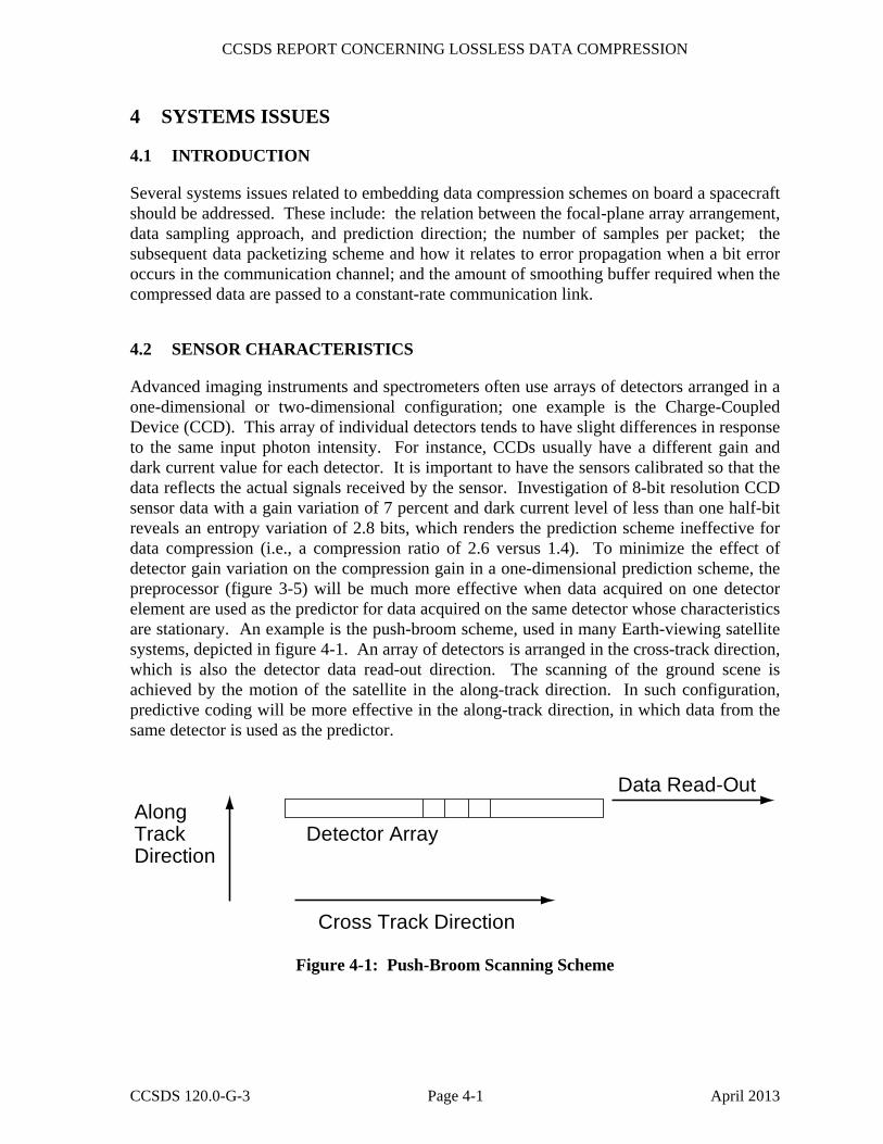
Advanced imaging instruments and spectrometers often use arrays of detectors arranged in a one-dimensional or two-dimensional configuration; one example is the Charge-Coupled Device (CCD). This array of individual detectors tends to have slight differences in response to the same input photon intensity. For instance, CCDs usually have a different gain and dark current value for each detector. It is important to have the sensors calibrated so that the data reflects the actual signals received by the sensor. Investigation of 8-bit resolution CCD sensor data with a gain variation of 7 percent and dark current level of less than one half-bit reveals an entropy variation of 2.8 bits, which renders the prediction scheme ineffective for data compression (i.e., a compression ratio of 2.6 versus 1.4). To minimize the effect of detector gain variation on the compression gain in a one-dimensional prediction scheme, the preprocessor (figure 3-5) will be much more effective when data acquired on one detector element are used as the predictor for data acquired on the same detector whose characteristics are stationary. An example is the push-broom scheme, used in many Earth-viewing satellite systems, depicted in figure 4-1. An array of detectors is arranged in the cross-track direction, which is also the detector data read-out direction. The scanning of the ground scene is achieved by the motion of the satellite in the along-track direction. In such configuration, predictive coding will be more effective in the along-track direction, in which data from the same detector is used as the predictor.

Cross Track Direction

AlongTrackDirection

Detector Array

Data Read-Out

Figure 4-1: Push-Broom Scanning Scheme



4.3 ERROR PROPAGATION

A major concern in using data compression is the possibility of error propagation in the event of a bit error, which can lead to a reconstruction error over successive data points. This effect can be reduced by packetization, to limit the extent of such error propagation, and channel coding such as Reed-Solomon coding, to reduce the probability of a channel error (see reference [7]). An example for space application would be to packetize the compressed data of one scan line in a CCSDS-recommended data packet format (reference [3]) and the compressed data of the next scan line into a second packet. In the case of a bit error in one packet, the decompression error would only propagate from the location of the error event to the end of the packet.

4.4 DATA PACKETIZATION AND COMPRESSION PERFORMANCE

The total number of encoded bits resulting from Losslessly compressing a fixed number of data samples is variable. The CCSDS data architecture provides a structure to packetize the variable-length data stream, which then can be put into a fixed-length frame to be transported from space to ground. Packetization is essential for preventing error propagation, as mentioned above; it also can affect the compression performance for the data set. To maximize the compression performance, packetization should be performed on several blocks to minimize the fraction of bits devoted to header overhead. However, to limit error propagation, a reasonable number of data blocks should be chosen for each packet.

There exist other available compression algorithms whose performance depends on establishing the long-term statistics of the collection of sensor data. Such schemes will in general give good compression performance for a large amount of data, and poor performance for a relatively small amount of data. And if packetization is used as a means of preventing error propagation in conjunction with these algorithms, one would expect poor performance for a shorter packet and a better performance for a larger packet. The drawback is that the loss of data due to error propagation may be intolerable for the larger packet.

Lossless data compression is not recommended for systems with fixed-length packets because the compression performance achieved is lower than that achieved with a variable-length packet system. For on-board designs that require fixed-length packets, the compressed data will be followed by fill bits to bring the packet to its fixed length. The quantity of fill bits added should insure that packet overflow is highly improbable. If the compressed bit count is greater than the fixed length, truncation occurs with loss of data. The decoder recognizes the truncation condition and signals when a block has been truncated by outputting dummy symbols. The decoder will output as many dummy symbols as would be in a typical packet that was not truncated. If one or more blocks were truncated, corresponding blocks of dummy symbols will be output to fill out the required blocks-per-packet. To lessen the effects of truncation when fixed-length packet structures are used, the design could be engineered so that the split k-bit Least Significant Bits (LSBs) are the last to be transmitted. In such an arrangement, if truncation occurs, probably only the LSBs would be lost, and thus the impact on performance would be lessened. However, for the packet, the compression is no longer Lossless.



4.5 BUFFER REQUIREMENT

Depending on the mission requirement, the variable-length packets resulting from packing the compressed bit stream into CCSDS packets can be stored in a large on-board memory, or they can be multiplexed with other data packets before being stored in the memory device. In either case, the large-capacity memory device lessens the variation in the packet length. Subsequent readout from the memory is performed at a fixed rate. In other situations, the variable-length packets may have to be temporarily buffered before a direct transmission to the communication link. The temporary buffer serves as a smoothing buffer for the link. Occasionally fill bits are inserted in the data stream to provide a constant readout rate. The amount of buffer needed is a function of the incoming packet rate, the packet length statistics, and the readout rate.

An analysis was conducted, using the CCSDS AOS Space Data Link Protocol (reference [4]), which examined issues such as the maximum smoothing buffer size requirement when a variable-rate Multiplexing Protocol Data Unit (MPDU) is transmitted to ground within a fixed-rate Virtual Channel Data Unit (VCDU). In this analysis, the MPDU transported variable-length packets with compressed data whose length varied with Gaussian statistics. Figure 4-2 shows the results of this analysis, where the probability of buffer overflow decreases as the buffer size increases. Doubling the buffer size normally will decrease the probability of buffer overflow by several orders of magnitude. The MPDUs are shifted asynchronously into the VCDU whenever they are filled, and thus the MPDU input to the VCDU occurs at a packet generation time period of tp, when it is available; ts represents the sampling period of the VCDU, which provides a constant data rate to the physical channel.



32

1

100

10-1

10-2

10-3

10-4

10-5

10-6

10-7

10-8

10-9

10-10

1.0 1.5 2.0 2.5 3.0 3.5 4.0 4.5

packet mean: 1.0 MPDUpacket σ: 0.2 MPDU1: ts/tp = 0.52: ts/tp = 0.753: ts/tp = 0.9

Pro

babi

lity

of E

xcee

ding

Buf

fer S

ize

Buffer Size, MPDU

Figure 4-2: Probability of Buffer Overflow



5 IMPLEMENTATION

5.1 OVERVIEW

The examples shown in this section are based on a system using the CCSDS AOS Space Data Link Protocol (reference [4]) in conjunction with the CCSDS Space Packet Protocol (reference [3]) and the CCSDS TM Synchronization and Channel Coding (reference [7]).

5.2 SPACE SEGMENT

Figure 5-1 represents the Space Segment as a functional block diagram that identifies each of the operations related to the data as they are transported through the CCSDS on-board layered architecture when Reed-Solomon error-correction is used. The following description assumes that the on-board instrument data to be compressed is a multispectral imager.

Multi-spectral

Instrument

SDU

SpectrumSelector

Lossless DataCompression

Unit

ChannelSelectorControl

InstrumentSubsystem

SDUCompressed

SDU

APIDControl

Time

Path PacketGenerator

PacketMultiplexer

OtherSourcePackets

CVCDUGenerator

Packet

Multiplexerand CADUGenerator

CADU

RadioFrequency

Router

OtherCVCDU

SelectRF Channel

To RFModulator

High-SpeedMultiplexerSubsystem

CVCDUMPDU

Application Layer Network Layer Data Link Layer Physical Layer

Figure 5-1: The Space Segment

In the Application Layer, spectral channels are selected for the images to be transported for intended users. The selector outputs Service Data Units (SDUs), which are metered out in scan lines as they are generated. There will be one SDU for each individual spectral channel (i.e., the scan lines for spectral channels are not multiplexed into a single SDU). Other functions of the Application Layer are to perform the data compression operation on the SDU and identify the length of the SDU to the nearest octet boundary before passing it to the path packet generator.

In the Network Layer, SDUs are tagged with appropriate Application Process Identifiers (APIDs) and packets are generated with the packet length signaled in the packet header. If time tagging is required, the secondary header flag is set, and time is inserted into the secondary header field. In the Data Link Layer, the image data packets are multiplexed with packets from other instruments into a fixed-length MPDU. The MPDU header contains the first packet header pointer, which is required for demultiplexing. These MPDUs are then assigned to a particular virtual channel in which Coded Virtual Channel Data Units (CVCDUs) of fixed-length units of octets are generated. The CVCDUs contain the sequence counter and the Reed-Solomon parity octets. These CVCDUs are then randomized to insure



bit transition and are passed on to the Multiplexer and Channel Assess Data Unit (CADU) generator. At this point, CADUs from other non-related instrument data are multiplexed together and are separated into selected channels to be routed to users.

5.3 GROUND SEGMENT

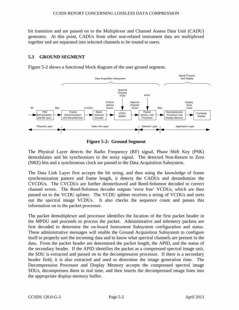
Figure 5-2 shows a functional block diagram of the user ground segment.

PSKDemodulationand Bit Sync.

FrameSynchronization

and Derandomizer

Reed-SolomonDecoder

VCDUSplitter

PacketDemux. andProcessor

DecompressionProcessor and

Display Memory

ComputerDisplay

Bits UDCVCFR

VCDUswithoutErrors

SpectralChannel

VCID

SpectralChannelVCDU

APID

SDU

DisplayScanLines

Signal Processand DisplayData Acquisition Subsystem

Application LayerNetwork LayerData Link LayerPhysical Layer

Figure 5-2: Ground Segment

The Physical Layer detects the Radio Frequency (RF) signal, Phase Shift Key (PSK) demodulates and bit synchronizes to the noisy signal. The detected Non-Return to Zero (NRZ) bits and a synchronous clock are passed to the Data Acquisition Subsystem.

The Data Link Layer first accepts the bit string, and then using the knowledge of frame synchronization pattern and frame length, it detects the CADUs and derandomize the CVCDUs. The CVCDUs are further deinterleaved and Reed-Solomon decoded to correct channel errors. The Reed-Solomon decoder outputs ‘error free’ VCDUs, which are then passed on to the VCDU splitter. The VCDU splitter receives a string of VCDUs and sorts out the spectral image VCDUs. It also checks the sequence count and passes this information on to the packet processor.

The packet demultiplexer and processor identifies the location of the first packet header in the MPDU and proceeds to process the packet. Administrative and telemetry packets are first decoded to determine the on-board Instrument Subsystem configuration and status. These administrative messages will enable the Ground Acquisition Subsystem to configure itself to properly sort the incoming data and to know what spectral channels are present in the data. From the packet header are determined the packet length, the APID, and the status of the secondary header. If the APID identifies the packet as a compressed spectral image unit, the SDU is extracted and passed on to the decompression processor. If there is a secondary header field, it is also extracted and used to determine the image generation time. The Decompression Processor and Display Memory accepts the compressed spectral image SDUs, decompresses them in real time, and then inserts the decompressed image lines into the appropriate display-memory buffer.



5.4 DECODING

The Lossless decoder consists of two separate functional parts, the post processor and the adaptive entropy decoder, as shown in figure 5-3. The postprocessor performs both the inverse prediction operation and the inverse of the standard mapper operation (see figure 3-5).

AdaptiveEntropyDecoder

Postprocessory x

Reference Flag

PacketStart Stop

ConfigurationParameters

Figure 5-3: Decoder Block Diagram

The first step toward decoding is to set up the configuration parameters so both encoder and decoder operate in the same mode. These configuration parameters will be mission specific and fixed for a given APID and are either known a priori or are signaled in the Compression Identification Packet (CIP).

The configuration parameters common to both encoder and decoder are:

– resolution in bits per sample (n = 1,..., 32);

– block size in samples (J = 8, 16, 32 or 64);

– number of Coded Data Sets (CDSes) contained in a packet (l = 1,..., 4096);

– number of CDSes between references (r = 1,..., 4096);

– predictor type if present;

– sense of digital signal value (positive or bipolar).

The inputs to the decoder are: a) the source packet data field containing the compressed source data y; b) the source packet data field start and stop signals, and c) the decoder configuration parameters.

The Adaptive Entropy Decoder utilizes the decoder configuration parameters to process the compressed variable-length data contained within the source packet data field.



The selected code-option ID bits, which are at the beginning of the CDS, will be extracted first. If a reference sample was inserted in the CDS during encoding, it will always appear in the first CDS of a packet and will re-appear after r CDSes if the packet length is greater than r. The reference word will be extracted next from the CDS bit stream and passed on to the postprocessor. Depending on the ID bits, the decoder will interpret the remaining bits in the CDS as coded bits by one of the options specified in reference [1].

For the No-Compression option, the remaining bits in the CDS will be passed to the postprocessor directly. For all other options, the FS codewords will be decoded as described in 3.2.1. For Split Sample options, each of the extracted J FS codewords will be concatenated with k split bits extracted from the stream using the CDS data format in 5.1.4 of reference [1].

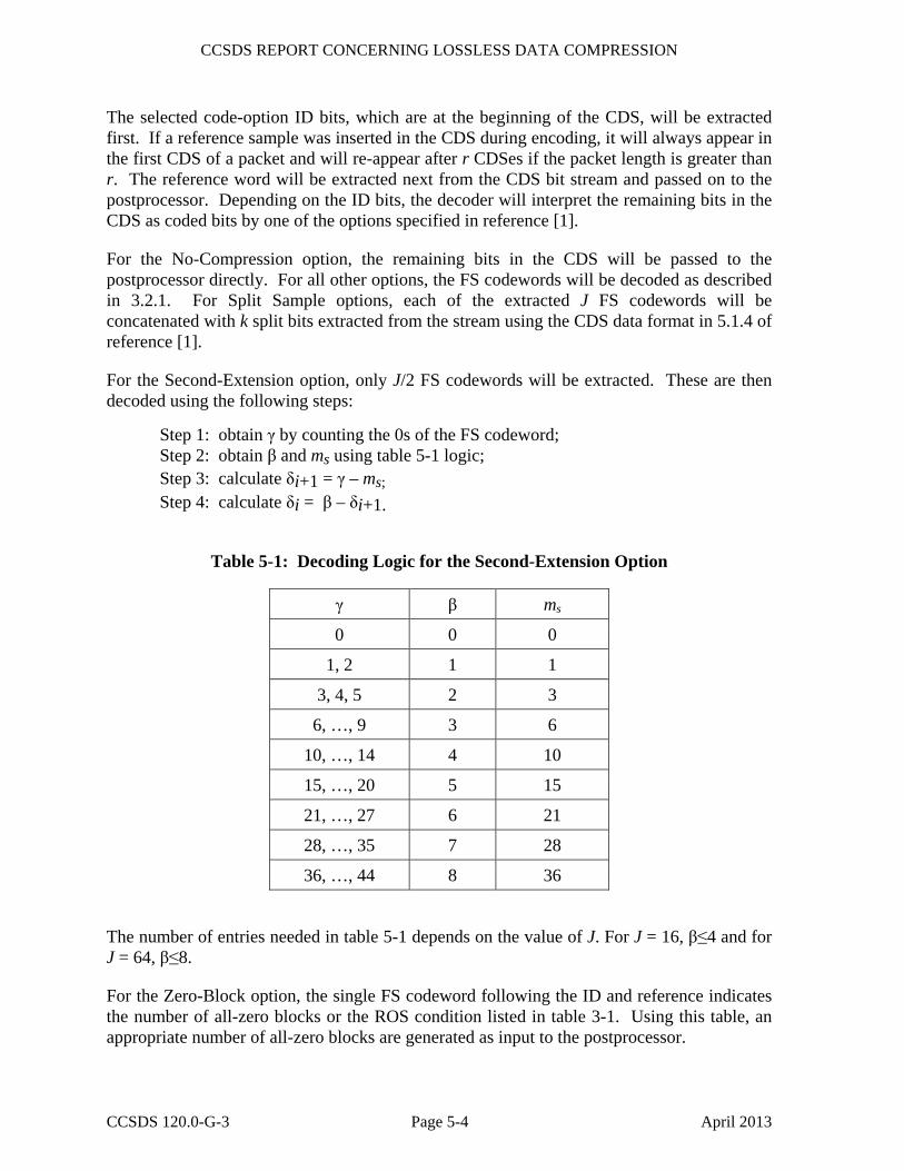
For the Second-Extension option, only J/2 FS codewords will be extracted. These are then decoded using the following steps:

Step 1: obtain γ by counting the 0s of the FS codeword; Step 2: obtain β and ms using table 5-1 logic; Step 3: calculate δi+1 = γ – ms; Step 4: calculate δi = β – δi+1.

Table 5-1: Decoding Logic for the Second-Extension Option

γ β ms

0 0 0

1, 2 1 1

3, 4, 5 2 3

6, …, 9 3 6

10, …, 14 4 10

15, …, 20 5 15

21, …, 27 6 21

28, …, 35 7 28

36, …, 44 8 36

The number of entries needed in table 5-1 depends on the value of J. For J = 16, β≤4 and for J = 64, β≤8.

For the Zero-Block option, the single FS codeword following the ID and reference indicates the number of all-zero blocks or the ROS condition listed in table 3-1. Using this table, an appropriate number of all-zero blocks are generated as input to the postprocessor.



The postprocessor reverses the mapper function, given the predicted value x̂i. When the preprocessor is not used during encoding, the postprocessor is bypassed as well. The inverse mapper function can be expressed as:

if δi ≤ 2θi,

Δi = δi/2 –( )δi + 1 /2

when δi is even when δi is odd

if δi > 2θi,

Δi = δi – θi θi – δi

when θi = x̂i – xmin when θi = xmax – x̂i

where θi = minimum (x̂i – xmin, xmax – x̂i)

There will be J (or J–1 for a CDS with reference sample) prediction error values Δ1, Δ2,....ΔJ generated from one CDS. These values will be used in the unit-delay postprocessor (figure 3-5) to recover the J sample values x1, x2,.....xJ.

To decode packets that may include fill bits, two pieces of information must be communicated to the decoder. First, the decoder must know the block size, J, and the number of CDSes in a packet, l. Second, the decoder must know when the Source Packet Data Field (SPDF) begins and when it ends. From these two pieces of information, the number of fill bits at the end of the data field can be determined.

The number of valid samples in the last CDS in the SPDF may be less than J. If so, the user will have added fill samples to the last CDS to make a full J-sample block, and the user must extract the valid samples from the last J-sample block.



6 PERFORMANCE

6.1 MEASURE

There are two measures of Lossless Data Compression performance: the encoded data rate, measured in bits per sample, and the processing time. The latter will not be addressed in this document, since it is highly dependent upon the processing engine.

The lowest data rate at which a source can be Losslessly represented is referred to as the entropy of the source. That is, a source with entropy of H bits per sample requires an average at least H bits to represent each sample. For example, if outputs from a discrete source are independent and identically distributed with probabilities p1, p2,....p(2n

–1), then the source has entropy:

H = – ∑0

2n –1 pi log2 pi

If the source outputs are not independent, then the entropy depends on higher-order probability distributions. Most real-world sources are sufficiently complex that it is impossible to compute the source entropy exactly, and thus the ultimate compression limit achievable on any source is usually unknown.

It is tempting to measure the first order probability distribution for a source and calculate the ‘first order’ entropy using the above expression. However, this approach produces an accurate estimate only if the output symbols are independent. By applying various Lossless compression techniques, an upper bound on the entropy of a source can be estimated. It is also possible to develop a probabilistic model of the source, and compute the entropy of the model.

The Compression Ratio (CR) is the ratio of the number of bits per sample before compression to the encoded data rate, so for the Lossless compression algorithm:

CR = nJ

average CDS length in bits

where n is the sample resolution and J is the block size.

Normally for imaging science data, the CR is approximately two. In the worst case, when the No-Compression option is selected, the resulting CR will be slightly less than one because of the ID overhead bits.

6.2 EXAMPLES

The following subsections contain compression-study results, most of which were extracted from reference [5], for eight different scientific imaging and non-imaging instruments. The compression performance, expressed as CR, is summarized in table 6-1. It should be noted that the CR is instrument-data dependent. For a specific instrument, the CR can vary from



one data set to the next. The reader should refer to each individual example following table 6-1 for more details on the instrument data set.

Table 6-1: Summary of Data Compression Performance for Different Scientific Data Sets

Paragraph Instrument Data Set Compression Ratio Imaging a) Thematic Mapper 1.83 b) Hyper Spectral Imager 2.6 c) Heat Capacity Mapping Radiometer 2.19 d) Wide Field Planetary Camera 2.97 e) Soft X-Ray Solar Telescope 4.69 Non-Imaging f) Goddard High Resolution Spectrometer 1.72 g) Acousto-Optical Spectrometer 2.3 h) Gamma-Ray Spectrometer 5 to 261

1 depending on integration time

a) Thematic Mapper (TM)

Mission Purpose: The Landsat program was initiated for the study of the Earth’s surface and resources. Landsat-1, Landsat-2, and Landsat-3 were launched between 1972 and 1978. Landsat-4 and Landsat-5 were launched in 1982 and 1984, respectively.

Landsat Thematic Mapper: on Landsat-4 and 5, the TM data represent typical land observation data acquired by projecting mirror-scanned imagery to solid-state detectors. The sensor for bands 1-5 is a staggered 16-element photo-diode array; it is a staggered 4-element array for band 6. An image acquired on Landsat-4 at 30m ground resolution for band 1 in the wavelength region of 0.45 - 0.52 μm is shown in figure 6-1. This 8-bit 512 x 512 image was taken over Sierra Nevada in California and has relatively high information over the mountainous area.

Compression Study: Using a unit-delay predictor in the horizontal direction, setting a block size of 16 samples, and inserting one reference per every image line, the Lossless compression gives a CR of 1.83 for the 8-bit image.

Figure 6-1: Landsat-4 Image



b) Hyper Spectral Imager on Small Satellite Technology Infusion Lewis Mission

Mission Purpose: The Small Satellite Technology Infusion (SSTI) mission objective is to transition to future missions new technologies which have significant measurable performance benefits. The mission will be launched in 1997.

Hyper Spectral Imager (HSI): The instrument contains three CCD arrays of detectors. Two of them are used to collect spectral-spatial information in the wavelength range from 0.4 to 2.5 μm: the Visible-Near-Infra-Red (VNIR) imager and the Short-Wave-Infra-Red (SWIR) imager. These imagers provide a 256 pixel spatial line with 128 spectral band information from the VNIR detector and 256 spectral bands from the SWIR detector. Both VNIR and

SWIR output are quantized to 12-bit data, and the ground resolution is 30m. The third CCD is a panchromatic imager which provides 5m ground resolution at 8-bit output. This CCD is a linear array of 2592 elements. Data compression will be applied only to the VNIR and SWIR data cubes, which are sets of 256 x 256 spatial information with 384 spectral information (see figure 6-2a).

Compression Study: Until actual in-strument data can be collected after the launch, the simulation is performed on a data cube simulated from Airborne Visible Infrared Imaging Spectrometer (AVIRIS) data. Compression is ap-plied to either VNIR or SWIR data separately but in the same manner, that is, along the spatial direction in a spatial-spectral plane shown in figure 6-2b. An average compression ratio of 2.6 was obtained over both the VNIR and SWIR data. If multispectral prediction is applied between the spectral lines, the CR is increased to 3.44. Figure 6-2c shows a spatial plane cut through the data cube.

256 spatial elements

384

wav

elen

gths

256

a spatial plane

Figure 6-2a:

An HSI Data Cube

Figure 6-2b: A VNIR Spatial-Spectral Plane

Figure 6-2c: A VNIR Spatial Plane



c) Heat Capacity Mapping Radiometer

Mission Purpose: Launched in 1978, the mission supported exploratory scientific investigations to establish the feasibility of utilizing thermal infrared remote sensor-derived temperature measurements of the Earth’s surface within a 12-hour interval, and to apply the night/day temperature-difference measurements to the determination of thermal inertia of the Earth’s surface.

Heat Capacity Mapping Radiometer: The sensor is a solid-state photo-detector sensitive in either the visible or the infrared region. A typical 8-bit image taken in the visible light region is given in figure 6-3, at a ground resolution of 500m over the Chesapeake Bay area on the U.S. East Coast.

Compression Study:

One-dimensional prediction: choosing unit-delay prediction in the horizontal direction, and setting block size J at 16, Lossless compression gives a CR of 2.19.

Two-dimensional prediction: using a two-dimensional predictor which takes the average of the previous sample and the sample on the previous scan line, and keeping other parameters the same, Lossless compression achieves a CR of 2.28, or about a 5% increase over a one-dimensional predictor.

Figure 6-3: Heat Capacity Mapping Radiometer Image



d) Wide Field Planetary Camera (WFPC) on Hubble Space Telescope

Mission Purpose: The Hubble Space Telescope (HST), launched in 1990, is aimed at acquiring astronomy data at a resolution never achieved before and observing objects that are 100 times fainter than other observatories have observed.

Wide Field Planetary Camera (WFPC): The camera uses four area-array CCD detectors. A typical star field observed by this camera is shown in figure 6-4. This particular image data has maximum value of a 12-bit resolution, which includes background noise of 9 bits.

Compression Study: Two studies were performed. The first was an investigation into Lossless compression performance on a thresholded star-field at various background noise levels. The second was a study of the effect on the compression ratio produced by varying the length of the source data to be compressed in a packet.

Threshold Study: The effect of thresholding a star field on the compression performance was explored in this study. Different threshold values were applied to this image and the values of the data were restricted to the threshold value or greater. The thresholding operation did not change the visual quality of the image. All the bright stars were unaffected. The resultant image was compressed Losslessly and the compression made use of the low-entropy option frequently over the image. The original image in figure 6-4 has a minimum quantized value of 423 and an array size of 800 x 800. The compression was performed using a block size of 16 and a unit-delay predictor in the horizontal line direction. Results are summarized in table 6-2.

Figure 6-4: Wide Field Planetary Camera Image



Table 6-2: Compression Ratio (CR) at Different Threshold Values

Threshold Values

CCSDS LDC LZW

None 2.97 3.30 430 2.99 3.33 440 11.92 17.15 450 41.20 63.53 460 53.52 91.48 470 63.66 110.73

In table 6-2, the CCSDS Lossless Data Compression (LDC) CRs for the WFPC study are compared with CRs obtained using the Lempel-Ziv-Welch (LZW) algorithm. Although the performance of the LZW algorithm over the whole image appears better than that of CCSDS Lossless Data Compression (LDC) algorithm, the results are reversed after considering the error propagation and packetization issues involved in implementing a Lossless algorithm.

Packetization Study: When a packet data format is used for the compressed data, it is expected that during decompression the reconstruction error caused by a single bit error in the packet will not propagate to the next packet, because the data packets are independent of each other and no code tables or statistics of data are passed from one packet to the next. To explore the effect of packet size on the compression performance, several individual lines from figure 6-4 are extracted and compressed separately. The results in table 6-3 are obtained on lines 101 through 104, which cover partially the brightest star cluster on the upper left corner of figure 6-4.

Table 6-3: Compression Ratio vs. Packet Size

Threshold Packet Size No. of Lines

CCSDS LDC LZW

None 1 (Line 101) 2.89 1.94 None 1 (Line 102) 2.90 1.92 None 1 (Line 103) 2.86 1.90 None 1 (Line 104) 2.88 1.90 None 2 (Line 101-102) 2.90 2.13 None 2 (Line 103-104) 2.87 2.09 None 4 (Line 101-104) 2.89 2.29 470 1 (Line 101) 16.24 6.98 470 1 (Line 102) 16.92 6.98 470 1 (Line 103) 15.42 6.94 470 1 (Line 104) 16.24 6.67 470 2 (Line 101-102) 16.45 8.70 470 2 (Line 103-104) 15.80 8.60 470 4 (Line 101-104) 16.06 10.30



e) Soft X-ray Telescope (SXT) on Solar-A Mission

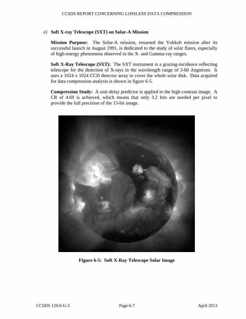
Mission Purpose: The Solar-A mission, renamed the Yohkoh mission after its successful launch in August 1991, is dedicated to the study of solar flares, especially of high-energy phenomena observed in the X- and Gamma-ray ranges.

Soft X-Ray Telescope (SXT): The SXT instrument is a grazing-incidence reflecting telescope for the detection of X-rays in the wavelength range of 3-60 Angstrom. It uses a 1024 x 1024 CCD detector array to cover the whole solar disk. Data acquired for data compression analysis is shown in figure 6-5.

Compression Study: A unit-delay predictor is applied to the high-contrast image. A CR of 4.69 is achieved, which means that only 3.2 bits are needed per pixel to provide the full precision of the 15-bit image.

Figure 6-5: Soft X-Ray Telescope Solar Image



f) Goddard High Resolution Spectrometer (GHRS) on Hubble Space Telescope

Mission Purpose: The Hubble Space Telescope (HST), launched in 1990, is aimed at acquiring astronomy data at a resolution never achieved before and observing objects that are 100 times fainter than other observatories have observed.

Goddard High Resolution Spectrometer (GHRS): The primary scientific objective of the GHRS instrument is to investigate the interstellar medium, stellar winds, evolution, and extra-galactic sources. Its sensors are two photo-diode arrays optimal in different wavelength regions, both in the UV range. Figure 6-6 gives examples of a typical spectrum and background trace. These traces have 512 data values; each is capable of storing digital counts in a dynamic range of 107. Spectral shapes usually do not vary greatly. However, subtle variations of the spectrum in such a large dynamic range presents a challenge for any Lossless data compression algorithm.

Compression Study: Two different prediction schemes are applied: the first uses the previous sample within the same trace and the second uses the previous trace in the same category (spectrum or background) as a predictor. The results are summarized below in table 6-4. The test data set contains data with a maximum value smaller than the 16-bit dynamic range, and the CR was thus calculated relative to 16 bits.

Table 6-4: Compression Ratio for GHRS

Trace Predictor CR Spectrum 1 Previous Sample 1.64 Spectrum 2 Previous Sample 1.63 Spectrum 2 Spectrum 1 1.72 Background 1 Previous Sample 2.51 Background 2 Previous Sample 2.51 Background 2 Background 1 1.53

Figure 6-6: Goddard High Resolution Spectrometer



g) Acousto-Optical Spectrometer on Submillimeter Wave Astronomy Satellite (SWAS)

Mission Purpose: The SWAS is a Small Explorer (SMEX) mission, scheduled for launch in 1998 aboard a Pegasus launcher. The objective of the SWAS is to study the energy balance and physical conditions of the molecular clouds in the galaxy by observing the radio-wave spectrum specific to certain molecules. It will relate these results to theories of star formation and planetary systems. The SMEX platform provides relatively inexpensive and shorter development time for the science mission. SWAS is a pioneering mission which packages a complete radio astronomy observatory into a small payload.

Acousto-Optical Spectrometer: The Acousto-Optical Spectrometer utilizes a Bragg cell to con-vert the radio frequency energy from the SWAS submillimeter wave receiver into an acoustic wave, which then diffracts a laser beam onto a CCD array. The sensor has 1450 elements with 16-bit readout. A typical spectrum is shown in figure 6-7(a). Expanded view of a portion of two spectral traces are given in figure 6-7(b). Because of the detector non-uniformity, the difference in the ADC gain between even-odd channel, and ef-fects caused by temperature variations, the spectra have non-uniform offset values between traces in addition to the saw-tooth shaped variation be-tween samples within a trace. Because of limited available on-board memory, a CR greater than 2 is required for this mission.

Compression Study: The large dynamic range and the variations within each trace present a challenge to the compression algorithm. Unit-delay prediction between samples is ineffective when the odd and even channels have different ADC gains. Three prediction modes are studied; the results are given in table 6-5.

The results show that, even with the similarity in spectral traces, a predictor using an adjacent trace in a direct manner will not improve the compression performance because of the uneven background offset. The multispectral predictor mode is especially effective in dealing with spatially registered multiple data sources with background offsets.

Figure 6-7: Acousto-Optical Spectrometer Waveform

Table 6-5: SWAS Compression Result

Predictor CR Previous Sample 1.58 Previous Trace 1.61 Previous Trace (Multispectral Higher Order Predictor)

2.32



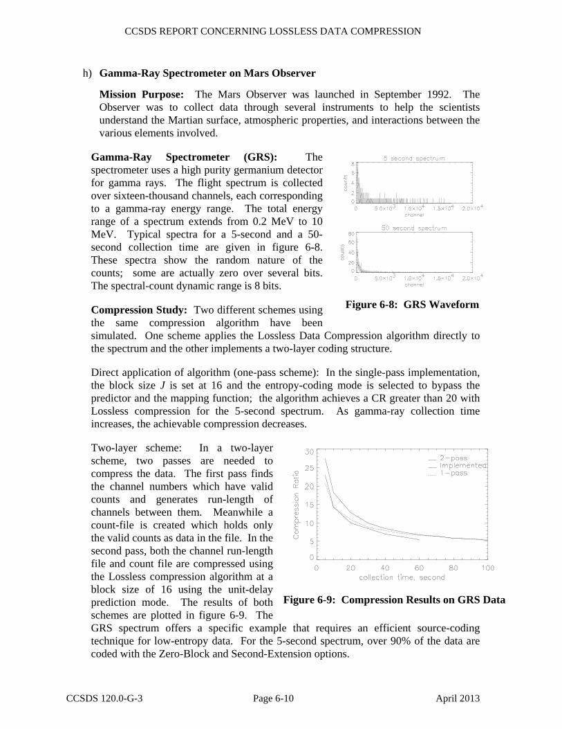
h) Gamma-Ray Spectrometer on Mars Observer

Mission Purpose: The Mars Observer was launched in September 1992. The Observer was to collect data through several instruments to help the scientists understand the Martian surface, atmospheric properties, and interactions between the various elements involved.

Gamma-Ray Spectrometer (GRS): The spectrometer uses a high purity germanium detector for gamma rays. The flight spectrum is collected over sixteen-thousand channels, each corresponding to a gamma-ray energy range. The total energy range of a spectrum extends from 0.2 MeV to 10 MeV. Typical spectra for a 5-second and a 50-second collection time are given in figure 6-8. These spectra show the random nature of the counts; some are actually zero over several bits. The spectral-count dynamic range is 8 bits.

Compression Study: Two different schemes using the same compression algorithm have been simulated. One scheme applies the Lossless Data Compression algorithm directly to the spectrum and the other implements a two-layer coding structure.

Direct application of algorithm (one-pass scheme): In the single-pass implementation, the block size J is set at 16 and the entropy-coding mode is selected to bypass the predictor and the mapping function; the algorithm achieves a CR greater than 20 with Lossless compression for the 5-second spectrum. As gamma-ray collection time increases, the achievable compression decreases.

Two-layer scheme: In a two-layer scheme, two passes are needed to compress the data. The first pass finds the channel numbers which have valid counts and generates run-length of channels between them. Meanwhile a count-file is created which holds only the valid counts as data in the file. In the second pass, both the channel run-length file and count file are compressed using the Lossless compression algorithm at a block size of 16 using the unit-delay prediction mode. The results of both schemes are plotted in figure 6-9. The GRS spectrum offers a specific example that requires an efficient source-coding technique for low-entropy data. For the 5-second spectrum, over 90% of the data are coded with the Zero-Block and Second-Extension options.

Figure 6-8: GRS Waveform

Figure 6-9: Compression Results on GRS Data


CCSDS 120.0-G-3 Page A-1 April 2013

ANNEX A

VERIFYING CCSDS LOSSLESS DATA COMPRESSION ENCODER IMPLEMENTATION

A1 PURPOSE

The objective of this annex is to present a limited set of test vectors to verify software or hardware implementations of the CCSDS Data Compression Encoder. This limited set of test vectors can be obtained from software that can be downloaded from the following location:

http://cwe.ccsds.org/sls/docs/sls-dc/

NOTE – The software and data are provided ‘as is’ to users as a courtesy. In no event will the CCSDS, its member Agencies, or the author of the software be liable for any consequential, incidental, or indirect damages arising out of the use of or inability to use the software.

A2 DESCRIPTION

The directory BB121B2TestData contains files for testing the CCSDS Lossless Data Compression Issue-2. The data sets will exercise all split-sample options, the no-compression option, the second-extension option as well as the zero-block option at least once. Test data covering the full dynamic range from n = 1 to 32 are included.


CCSDS 120.0-G-3 Page B-1 April 2013

ANNEX B

ACRONYMS AND ABBREVIATIONS

AOS Advanced Orbiting System

APID Application Process Identifier

AVIRIS Airborne Visible Infrared Imaging Spectrometer

CADU Channel Access Data Unit

CCD Charge Coupled Device

CCSDS Consultative Committee for Space Data Systems

CDS Coded Data Set

CR Compression Ratio

CVCDU Coded Virtual Channel Data Unit

FS Fundamental Sequence

GHRS Goddard High Resolution Spectrometer

GRS Gamma-Ray Spectrometer

HSI Hyper Spectral Imager

HST Hubble Space Telescope

LDC Lossless Data Compression

LSB Least Significant Bit

LZW Lempel Ziv Welch

MPDU Multiplexing Protocol Data Unit

NRZ Non-Return to Zero

pdf Probability Distribution Function

PSK Phase Shift Key

RF Radio Frequency

ROS Remainder-of-Segment

SDU Service Data Units


CCSDS 120.0-G-3 Page B-2 April 2013

SMEX Small Explorer

SPDF Source Packet Data Field

SSTI Small Satellite Technology Infusion

SWAS Submillimeter Wave Astronomy Satellite

SWIR Short-Wave-Infra-Red

SXT Soft X-Ray Telescope

TM Thematic Mapper

VCDU Virtual Channel Data Unit

VNIR Visible-Near-Infra-Red

WFPC Wide Field Planetary Camera

Lossless Data Compression - CCSDS.org · CCSDS REPORT CONCERNING LOSSLESS DATA COMPRESSION CCSDS...

Documents

Transcript of Lossless Data Compression - CCSDS.org · CCSDS REPORT CONCERNING LOSSLESS DATA COMPRESSION CCSDS...