Loop monitoring and assessment of hot strip mill controle00_obl/thesis.pdf · Loop monitoring and...
82
Loop monitoring and assessment of hot strip mill control OSCAR BLOMKVIST Master’s Thesis at the Dept. of Signals, Sensors & Systems Supervisor: Karl Werner Examiner: Magnus Jansson TRITA xxx yyyy-nn
-
Upload
hoangkhuong -
Category
Documents
-
view
217 -
download
2
Transcript of Loop monitoring and assessment of hot strip mill controle00_obl/thesis.pdf · Loop monitoring and...

Loop monitoring and assessmentof hot strip mill control
OSCAR BLOMKVIST
Master’s Thesis at the Dept. of Signals, Sensors & SystemsSupervisor: Karl Werner
Examiner: Magnus Jansson
TRITA xxx yyyy-nn


iii
Abstract
The object of the thesis work was to test assessment and monitoring tools for the controlof a hot strip rolling mill. Two control system were also evaluated, work roll bending controland gap control. The effectiveness of a filter, that is used within the control to remove theeffect of eccentric rolls, were analyzed.
Three monitoring and assessment methods where tested on 120 rolling operations, oneof these methods was Harris index. An evaluation of the control where performed withthe use of Harris index and parametric models of the closed loop control systems. Theeffectiveness of the eccentric roll filter where analyzed with spectrum analysis.
The results showed that the suggested methods could be used as monitoring tools, buthad different properties. Low time resolution in the measurements made some of the resultshard to interpret. It could be shown that the eccentricity filter did not remove the effect ofeccentric rolls completely and that the filter could be improved by adding a filter for ellipticrolls. The assessment of the control loops showed that they were stable and well tunedwithin the control structure. An overhaul of the reference limitations, reference generationand the estimation of the gap, has to be made if the control is to be improved.
Keywords: Harris index, loop monitoring, control assessment, eccentric rolls, hot stripmill, model prediction error, control error, oscillation, hydraulic valves.

iv
Sammanfattning
Målet med detta examensarbete har varit att testa metoder för utvärdering och över-vakning av reglerfunktioner i ett varmvalsverk. Två reglersystem har utvärderats, valsböjn-ingsreglering och valsspaltsreglering. Hur väl regleringens metod för att undvika effekternaav excentriska valsar undersöktes också.
Tre metoder för utvärdering och övervakning testades på 120 valsningar, en av dessametoder var Harris index. En utvärdering av reglering genomfördes där Harris index ochparametriska modeller av det slutna systemet användes. Funktionaliteten i metoden för attundvika effekterna av excentriska valsar analyserades med hjälp av spektralanalys.
Resultaten visade att de föreslagna metoderna för övervakning av reglering fungeradeoch hade olika egenskaper. Låg samplingshastighet i mätningarna gjorde att en del avresultaten var svåra att tyda. Det kunde visas att metoden för att ta bort effekten av ex-centriska valsar hade brister och att det fanns möjlighet till förbättringar. Utvärderingenvisade att regleringen var stabil och väl inställd inom den givna reglerstrukturen. För attkunna förbättra regleringen skulle en översyn av genereringen av referenser, begränsningenav referenssignaler och beräkningen av det skattade valsspalten, vara nödvändig.
Nyckelord: Harris index, övervakning, utvärdering, reglering, excentriska valsar, varm-valsverk, modellavvikelse, reglerfel, oscillering, hydrauliska ventiler.

Contents
Contents v
1 Introduction 11.1 Reading directions . . . . . . . . . . . . . . . . . . . . . . . . . . . . 11.2 Background . . . . . . . . . . . . . . . . . . . . . . . . . . . . . . . . 21.3 Difficulties in control of rolling mills . . . . . . . . . . . . . . . . . . 21.4 Hot strip mills . . . . . . . . . . . . . . . . . . . . . . . . . . . . . . 31.5 The steckel mill in Avesta . . . . . . . . . . . . . . . . . . . . . . . . 41.6 Automatic Gage Control (AGC) . . . . . . . . . . . . . . . . . . . . 61.7 Hydraulic Gap Control (HGC) . . . . . . . . . . . . . . . . . . . . . 71.8 Work Roll Bending (WRB) . . . . . . . . . . . . . . . . . . . . . . . 91.9 The roll eccentricity filter . . . . . . . . . . . . . . . . . . . . . . . . 111.10 The importance of monitoring systems in industrial processes . . . . 121.11 Production and Process Monitoring System (PPMS) . . . . . . . . . 131.12 Harris index . . . . . . . . . . . . . . . . . . . . . . . . . . . . . . . . 13
2 Problem definition 152.1 Assessment and monitoring tools for control loops . . . . . . . . . . 152.2 Harris index in HSM control . . . . . . . . . . . . . . . . . . . . . . . 162.3 Assessment of control loops . . . . . . . . . . . . . . . . . . . . . . . 162.4 Reasons for oscillations other than oscillating control loops . . . . . 17
2.4.1 Work roll eccentricity . . . . . . . . . . . . . . . . . . . . . . 172.4.2 Thickness measurement feedback oscillations . . . . . . . . . 17
3 Proposed solutions 193.1 Assessment and monitoring tools for control loops . . . . . . . . . . 19
3.1.1 Quadratic control error . . . . . . . . . . . . . . . . . . . . . 193.1.2 Model prediction error . . . . . . . . . . . . . . . . . . . . . . 20
3.2 Harris index in HSM control . . . . . . . . . . . . . . . . . . . . . . . 213.2.1 Method outlined by Harris . . . . . . . . . . . . . . . . . . . 213.2.2 Implementation in Avesta’s HSM . . . . . . . . . . . . . . . . 223.2.3 Dead time estimation . . . . . . . . . . . . . . . . . . . . . . 23
3.3 Assessment of control loops . . . . . . . . . . . . . . . . . . . . . . . 24
v

vi CONTENTS
3.4 Reasons for oscillations other than oscillating control loops . . . . . 243.4.1 Work roll eccentricity . . . . . . . . . . . . . . . . . . . . . . 243.4.2 Thickness measurement feedback oscillations . . . . . . . . . 26
4 Implementation 274.1 Assessment and monitoring tools for control loops . . . . . . . . . . 27
4.1.1 Quadratic control error . . . . . . . . . . . . . . . . . . . . . 274.1.2 Model prediction error . . . . . . . . . . . . . . . . . . . . . . 28
4.2 Harris index in HSM control . . . . . . . . . . . . . . . . . . . . . . . 294.2.1 Implementation in Avesta’s HSM . . . . . . . . . . . . . . . . 294.2.2 Dead time estimation . . . . . . . . . . . . . . . . . . . . . . 30
4.3 Assessment of control loops . . . . . . . . . . . . . . . . . . . . . . . 304.4 Reasons for oscillations other than oscillating control loops . . . . . 31
4.4.1 Roll eccentricity . . . . . . . . . . . . . . . . . . . . . . . . . 314.4.2 Thickness measurement feedback oscillations . . . . . . . . . 32
5 Results 355.1 Assessment and monitoring tools for control loops . . . . . . . . . . 36
5.1.1 Quadratic control error . . . . . . . . . . . . . . . . . . . . . 365.1.2 Model prediction error . . . . . . . . . . . . . . . . . . . . . . 38
5.2 Harris index in HSM control . . . . . . . . . . . . . . . . . . . . . . . 405.2.1 Dead time estimation . . . . . . . . . . . . . . . . . . . . . . 405.2.2 Work roll bending . . . . . . . . . . . . . . . . . . . . . . . . 435.2.3 Hydraulic gap control . . . . . . . . . . . . . . . . . . . . . . 445.2.4 Strip thickness measurement . . . . . . . . . . . . . . . . . . 475.2.5 WRB outliners . . . . . . . . . . . . . . . . . . . . . . . . . . 48
5.3 Assessment of control loops . . . . . . . . . . . . . . . . . . . . . . . 495.3.1 WRB control . . . . . . . . . . . . . . . . . . . . . . . . . . . 505.3.2 HGC control . . . . . . . . . . . . . . . . . . . . . . . . . . . 51
5.4 Reasons for oscillations other than oscillating control loops . . . . . 535.4.1 Roll eccentricity . . . . . . . . . . . . . . . . . . . . . . . . . 535.4.2 Thickness measurement feedback oscillations . . . . . . . . . 54
6 Conclusions 576.1 Assessment and monitoring tools . . . . . . . . . . . . . . . . . . . . 576.2 Harris index in roll control . . . . . . . . . . . . . . . . . . . . . . . . 576.3 Assessment of control loops . . . . . . . . . . . . . . . . . . . . . . . 586.4 Reasons for oscillations other than oscillating loops . . . . . . . . . . 59
7 Future work 617.1 Research . . . . . . . . . . . . . . . . . . . . . . . . . . . . . . . . . . 617.2 Avesta HSM . . . . . . . . . . . . . . . . . . . . . . . . . . . . . . . . 61
A Glossary (Ordlista) 65

vii
B Notation 67B.1 Acronyms . . . . . . . . . . . . . . . . . . . . . . . . . . . . . . . . . 67B.2 Abbreviations . . . . . . . . . . . . . . . . . . . . . . . . . . . . . . . 68
C The hydraulic systems 69
D Significance tests 71D.1 Measurements form the last pass of rolling . . . . . . . . . . . . . . . 71D.2 Measurements form the whole rolling . . . . . . . . . . . . . . . . . . 72
Bibliography 73


Chapter 1
Introduction
The aim of this master’s thesis is to develop monitoring and assessment tools forthe control loops in a hot strip mill (HSM). The tools should be general and be usedto make an assessment of the roll gap control and bending control. Three differenttools are tested, among them Harris index. Reasons for oscillations in the controlloops are investigated.
The work has been carried out at Outokumpu’s hot strip steckel mill in Avesta.Outokumpu’s facilities in Avesta hold all the plants necessary in the process ofmaking stainless steel out of scrap-metal.
The results showed that the suggested methods could be used as monitoringtools, but had different properties. Low time resolution in the measurements madesome of the results hard to interpret. It could be shown that the eccentricity filterdid not remove the effect of eccentric rolls completely and that the filter could beimproved by adding a filter for elliptic rolls. The assessment of the control loopsshowed that they were stable and well tuned within the control structure. Anoverhaul of the reference limitations, reference generation and the estimation of thegap, has to be made if the control is to be improved.
1.1 Reading directions
This first chapter is an introduction. The main focus is the gap and bending con-troller at Avesta steckel mill. The introduction will cover the different control mod-ules included in this thesis, the importance of monitoring tools, difficulties in rollingand also give a short presentation to hot strip rolling. For further reading on hotstrip mills and hot rolling [1] and [2] are recommended.
A problem definition is given in chapter 1. It describes the problems to be solvedand the assumptions that have been made. A motivation to why the problem isrelevant will also be presented. It is divided into four subsections. The first twosubsections covers monitoring and assessment tools for the control. The third coversthe assessment of control and the fourth covers oscillation in control loops. Theassessment of the control has a separate subsection to make the difference between
1

2 CHAPTER 1. INTRODUCTION
the assessment tools and the assessment more clear.The subsections have the same division in chapters 4-6 to simplify reading.Theoretical solutions to the defined problems are suggested in chapter 2. Imple-
mentation of the theoretical solutions are described in chapter 3. Implementationwill be made in Matlab (version 6.0.0.88), from MathWorks. The methods are de-signed to be possible to implement in the control system in the future. Results arepresented in chapter 5 and conclusions are drawn in chapter 6.
Future work in research and at Avesta steckel mill are discussed in chapter 7.This thesis includes both evaluation of suggested tools for monitoring and as-
sessment of control loops and an evaluation of the control. To avoid confusion itmight be good to keep this in mind when reading. The two parts have been dividedinto different subsections throughout the thesis to simplify reading.
A glossary with translations from English to Swedish are enclosed in the ap-pendix.
The structure of this thesis follows requirements and guidelines [3] from thedepartment of Signals, Sensors and Systems at KTH.
1.2 BackgroundAvestas hot strip mill make thin stainless steel strips between 2.5 and 12.5 mmthick, up to 2200 mm wide and up to 1000 meter long. The strip is made fromcasted steel slabs and rolled in two stands down to desired thickness.
The first stand is a conventional roughing mill. The last stand is a steckel mill.It is a special rolling technique that is only used in a small number of hot strip millsin the world. When this special technique is used, the demand on the control ishigh.
The demand on the control also gets higher because of demands on higher prod-uct quality. To ensure good control the need for an improvement of the monitoringsystems has been acknowledged.
There is a need to assess control performance itself and to acquire more knowl-edge on what effect disturbances and failing components has on the control perfor-mance. Detection of failure and deterioration in actuators, sensors and mechanicalparts enables good maintenance strategies and reduces unscheduled stops in theproduction.
1.3 Difficulties in control of rolling millsThe environment in a hot strip mill is very harsh. Heat, vibrations, large forces anddust are constantly affecting equipment such as actuators and sensors. A failingsensor or a leaking hydraulic valve may have large impact on control performance.
Evaluation of loop performance and the condition of actuators, sensors andmechanical parts are important in a maintenance as well as from a process analyzingperspective.

1.4. HOT STRIP MILLS 3
Figure 1.1. Schematic picture of the roughing stand.
Figure 1.2. Schematic picture of one of the heating furnaces.
The process is influenced by a large number of noise sources such as inhomoge-neous material, inhomogeneous temperature in materials, friction between movingparts, wear on rolls, heat expansion, roll defects from grindning, sensor faults andmany more. These noise sources are not measured in the plant and their behavioris often both unknown and time varying.
1.4 Hot strip mills
The objective in a hot strip mill (HSM) is to roll thick slabs into thin strips. Slabsare ingots of alloy metal that are produced in a continuous casting plant. Theslabs rolled in Avesta have been manufactured in Tornio (Finland), Sheffield (GreatBritain) and Avesta. They have a length of up to 11 meter, a thickness between 80and 220 mm and a width of up to 2050 mm.
Two furnaces are used to heat slabs. A picture of a furnace can be seen infigure 1.2. When they reach a temperature of 1250 °C they are lifted out of thefurnace on to the roller table. Roller tables are used throughout the plant to moveslabs and strips. The automation system guides the slab through the first stand,which is called a roughing mill stand. See figure 1.1.
There are different ways to make thin strip in a hot strip mill. In Avesta theprocess of thinning the strip is divided between the roughing mill and the steckelmill. When the slab exits the roughing mill it has to have a thickness of less then32 mm to enter the steckel mill. To be able to go from a thickness of 220 mm down

4 CHAPTER 1. INTRODUCTION
Figure 1.3. Schematic picture of the steckel mill with coilers and furnaces.
to 32 mm the slab has to be rolled several times, called passes. The slab is guidedby the automation system backward and forward and totally rolled five, seven ornine times depending on the material and the slab thickness.
When the slab exits the roughing mill it is roughly 80 meters long and is nowcalled a strip.
The steckel mill makes the final thinning of the strip down to desired thickness,which can vary between 2.5-12.5 mm. After exiting the steckel mill the strip iscooled with water and coiled to a roll. The roll is either sent to the customer orprocessed further at the cold rolling mill
1.5 The steckel mill in AvestaThe steckel mill rolls a hot strip from a thickness between 25-32 mm down to thedesired thickness between 2.5-12.5 mm. To make that reduction the strip has tobe rolled several times. In tandem plants, a number of stands are built after eachother. It enables a high production rate but has high establishment cost. Anothersolution is to guide the strip backwards and forwards through the stand, like in theroughing stand. This method is used in a steckel mill. Because there is only onestand it has a lower establishment cost but has on the other hand a lower productionrate.
Two problems arise if a strip is brought backwards and forwards through a millstand. As time goes it becomes colder and with that tougher and harder to roll. Italso becomes longer, up to a kilometer. To solve these two problems the steckel millhas two coilers, one on either side of the stand. To prevent the strip from becomingto cool each coiler is placed in a furnace. See figure 1.3.
Because the steckel mill is the finishing stand the exiting strip has to live upto certain quality conditions when the rolling is finished, this means that there aredemands on high performance and accuracy in the rolling. A number of control andcompensation modules are used in the mill to be able to manage this. They aredescribed in section 1.6, 1.7 and 1.8.
A picture of a four-high roll stand is shown in figure 1.4. The picture shows the
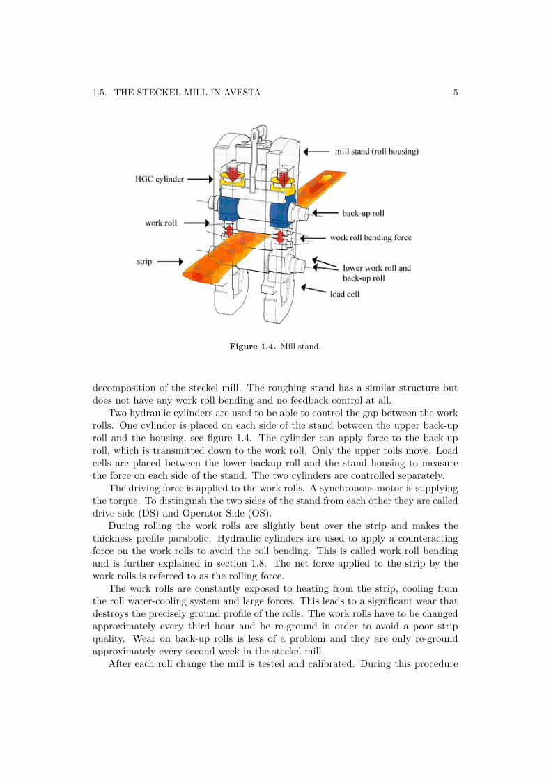
1.5. THE STECKEL MILL IN AVESTA 5
Figure 1.4. Mill stand.
decomposition of the steckel mill. The roughing stand has a similar structure butdoes not have any work roll bending and no feedback control at all.
Two hydraulic cylinders are used to be able to control the gap between the workrolls. One cylinder is placed on each side of the stand between the upper back-uproll and the housing, see figure 1.4. The cylinder can apply force to the back-uproll, which is transmitted down to the work roll. Only the upper rolls move. Loadcells are placed between the lower backup roll and the stand housing to measurethe force on each side of the stand. The two cylinders are controlled separately.
The driving force is applied to the work rolls. A synchronous motor is supplyingthe torque. To distinguish the two sides of the stand from each other they are calleddrive side (DS) and Operator Side (OS).
During rolling the work rolls are slightly bent over the strip and makes thethickness profile parabolic. Hydraulic cylinders are used to apply a counteractingforce on the work rolls to avoid the roll bending. This is called work roll bendingand is further explained in section 1.8. The net force applied to the strip by thework rolls is referred to as the rolling force.
The work rolls are constantly exposed to heating from the strip, cooling fromthe roll water-cooling system and large forces. This leads to a significant wear thatdestroys the precisely ground profile of the rolls. The work rolls have to be changedapproximately every third hour and be re-ground in order to avoid a poor stripquality. Wear on back-up rolls is less of a problem and they are only re-groundapproximately every second week in the steckel mill.
After each roll change the mill is tested and calibrated. During this procedure

6 CHAPTER 1. INTRODUCTION
Figure 1.5. A simpified picture of the control system
a number of variables are measured and calculated to detect anomalies. This isfurther described in section 1.11.
The rolling mill technology supplier German SMS Demag delivers the controlsystem of the mill. The implementation of the control is called technological controlsystem (TCS) and runs on a multi-bus computer system.
1.6 Automatic Gage Control (AGC)
The control of the gap between the work rolls, and in other words the strip thickness,is made in two steps with two control modules. See figure 1.5. The first module iscalled Automatic Gage Control (AGC). It receives thickness set points, s0, from ahigher-level system.
The AGC compensates for such things as roll wear, heat expansion in the rolls,stretch of the stand and other unmeasurable quantities which affects the gap. Thesequantities are all calculated using models and summed into a total gap deviation.
There is no thickness feedback control in the Hydraulic Gap Control (HGC).A thickness measurement is made during the passes, but is not used in the HGC.Instead it is used in the AGC. The thickness feedback is passed through a PI-controller and added to the total gap deviation. It can be seen as a model errorcompensation. This compensation will change the cylinder position reference in theHGC, further explained in section 1.7.
The total compensation, ∆s, calculated in the AGC is sent together with theset points received from the higher-level system to the HGC.

1.7. HYDRAULIC GAP CONTROL (HGC) 7
Figure 1.6. General signal scheme of the control system with a additive noise onthe output.
1.7 Hydraulic Gap Control (HGC)The HGC is the second module in the gap control, controlling the gap betweenthe two work rolls. The HGC uses the higher-level set points as roll gap referencevalues. Measurements from position transducers on the cylinders and the currentcompensation are used to calculate the true roll gap. The HGC is position controlledand uses the reference and the true gap to control the strip thickness.
A simplified description of the hydraulic system for the HGC is enclosed in theappendix.
To close or widen the gap, the HGC steers the servo valves for the hydrauliccylinders. The opening or closing of the valves will increase or decrease the rollingforce. The signal from the load cells gives a good approximation of the size of therolling force and is used in the AGC to calculate the gap compensation. There aretwo position transducers on each of the hydraulic cylinders that are measuring thecylinder stroke.
The hydraulic gap control is implemented as a PI-controller. Both the reference,r[n], and the control signal, c[n], are ramped and have an upper limit. This meansthat the signal has a maximum value and that the rate of increase is limited. Thisis done to avoid heavy strains on the mechanical parts.
The system can be described as a traditional control system, see figure 1.6.Because the control is implemented on computers and all measurements are sampledit is natural to describe the system with discrete time models. The hysteresis effectand the effect of ramping and limiting are disregarded and the system is assumedto be linear. This will be further discussed in chapter 2
y[n] = sc + ∆s (1.1)r[n] = s0 (1.2)
ε[n] = s0 − sc −∆s (1.3)Signal y[n] is the true roll gap and have been calculated from cylinder stroke
measurements and AGC compensation, see equation 1.1. A control error, ε[n], is

8 CHAPTER 1. INTRODUCTION
Figure 1.7. The reference of the gap during rolling. The strip has been rolled inseven passes in this example.
Figure 1.8. Closeup of the reference and actual gap during the last pass of rolling.
calculated by subtracting the true roll gap from the reference value r[n], which alsohave been received from the AGC, see equation 1.3. The control error is fed to thePI controller, A(q−1)
B(q−1). The output of the control is the control signal, c[n], which
steers the valves to the cylinder. The valves are opened when the control signalincrease, which leads to a higher pressure in the cylinder. This in turn leads toa larger force, which reduces the gap. The box containing, C(q−1)
D(q−1), describes the
system between the control signal and the true gap, that is the mill. This includescylinder, valve and stand dynamics.
A noise is added to the output, y[n]. The noise is described as filtered whitenoise, e[n], where is the filter. The noise represents disturbances such as temperaturevariation in the strip, friction, metallurgical variations in the strip, model errors andso on.
Typical reference and actual gap value can be seen in figure 1.7 and figure 1.8.

1.8. WORK ROLL BENDING (WRB) 9
1.8 Work Roll Bending (WRB)
As noted in section 1.4 the backup rolls have a large dimension to support the workroll and prevent them from bending. In spite of this the backup rolls will be bentwhen the force on the bearing housing becomes large. This will make the forceapplied on the work roll higher closer to the bearing housing and smaller at themiddle of the roll. The strip on the other hand will operate with a reactive force.This force will be acting onto the middle of the roll. This will bend the work rolland affect the profile of the strip, see figure 1.9.
The work roll bending system enables profile shaping of the strip by applying acounteracting force on the work rolls bearing housings. When a large bending forceis applied the profile will become more flat.
The bending force is constantly changing and the reference force is calculatedas a function of the rolling force. Four hydraulic cylinders on each side generatethe force. The work roll bending system has a force control. Because there are noforce measurements available the force has to be calculated from the pressure incylinders.
Another way to change the strip profile is to use rolls with a profile. The gapbetween the rolls can be changed by the use of a "smart" profile together with axialshifting of the rolls. The "smart" profile used is called a CVC-curve (continuousvariable crown) and the technique is called roll shifting. See figure 1.10.
Roll shifting has slower dynamics than work roll bending but a larger range,they complement each other and both systems are used in the steckel mill.
In contrast to what one might think the optimal profile is not a complete flatprofile. In the continuing process (that is cold rolling) the strip has to have a certainamount of profile to be processed. The customer often buys products with demandson the least thickness. This, on the other hand, makes it more profitable to have asflat profile as possible in order to save material. These incompatible wishes makeit important to have a good work roll bending control to get as close as possible tothe optimal profile.
The work roll bending is implemented in the TCS as a PI-controller. It is forcecontrolled. The control can be described as the HGC in the previous section. Seefigure 1.6.
The true value, y[n], is the true force calculated from the hydraulic pressure atcylinder and rod side of the cylinders. The system can be described in the sameway as the HGC. It has a PI-controller, A(q−1)
B(q−1), some dynamics, C(q−1)
D(q−1), and noise,
E(q−1)F (q−1)
.Examples of the reference and true values of the bending force can be seen in
figure 1.11 and figure 1.12.

10 CHAPTER 1. INTRODUCTION
Figure 1.9. Schematic picture of forces during rolling.
Figure 1.10. Shifting of work rolls with a CVC-curve. Note how the strip profilechange.
Figure 1.11. The reference force for the WRB during rolling of one strip.

1.9. THE ROLL ECCENTRICITY FILTER 11
Figure 1.12. Closeup of the reference and true force of the WRB during rolling.
1.9 The roll eccentricity filter
The gap control system is designed to follow a reference position at the cylinder,as described in section 1.7. If, for example, the strip is cooler at some point therolling force will not be sufficient to keep the cylinder position. The control systemwill increase the rolling force when the deviation from the reference is detected toget back to the reference position.
This control strategy is necessary to control the thickness, not only because oftemperature differences over the strip but also for other disturbances such as frictionin the mill or inhomogeneous material. It has drawbacks, however.
An eccentric roll will make the distance between the cylinder and the strip vary.These variations are not included in the reference value and are thereby consideredas a disturbance by the controller. To keep the reference position, the controller willincrease the rolling force and reduce strip thickness. The increased force will leadto a stretch in the mill. A compensation for the mill stretch is always calculatedin the AGC and added to the reference. This will further increase the deviation incylinder position and make the controller increase the force even more.
To avoid the extra force increase the reference value should not change becauseof roll eccentricity. The stretch compensation signal is therefore filtered throughtwo notch filters. They are designed to eliminate one frequency component from asignal. One notch filter will filter away the same frequency as the work roll rotation,the other will filter away the same frequency as the backup roll rotation.
The stand is with other words allowed to spring when the springing is causedby roll eccentricity. This make the gap between the work rolls to vary less duringload.

12 CHAPTER 1. INTRODUCTION
1.10 The importance of monitoring systems in industrialprocesses
Maintenance strategies have for long been an issue [4] in the industrial community.Strategies for maintenance can be divided in to three different categories, whichalso represent the development of maintenance strategies.
The first strategy is more or less an absence of strategy. It is called "damagebased maintenance". Nothing is done until the device fail. This is expensive be-cause preventive maintenance could give the device a longer life. It also leads tounscheduled breaks in the production, which lowers the availability. This is espe-cially important in hot strip mills there the whole production line must work toenable production. There is also a risk that a failing device may damage otherequipment.
The second strategy is "time based maintenance". It means that devices arechecked and maintained at predefined time intervals. This is a naive approach thatmight sound as quite good but has drawbacks. The deterioration of a device is avery stochastic process. The variance in the time before failure is very large formost components which makes it hard to have appropriate maintenance intervals.To short intervals leads to unnecessary maintenance and to long may lead to devicefailure [4].
The most recently suggested strategy is having "condition based maintenance".It means that the condition of a device is monitored. The monitoring system usesmeasurements to evaluate the condition and advises the operator on appropriateaction to avoid failure or further deterioration.
It is obvious that the last strategy is preferred. It keeps maintenance costs lowbecause no unnecessary maintenance is made and devices are changed before failureand thereby avoiding unnecessary hold-ups in the production.
There are often as many as hundreds of control loops in process plants [5] andmany of those have poor tuning [6]. It is important to have tools that are easy toimplement to be able to monitor many control loops.
Deterioration in a sensor or an actuator will have an impact on control per-formance. A deficiency in control performance will inevitably lead to poor stripquality. Monitoring of control loops is important to avoid poor strip quality and away to get indications on the condition of sensors and actuators.
In Avestas hot strip mill it is important to avoid any unscheduled breaks in theproduction, especially during high order intake. Unscheduled breaks are destroyingdelivery time to following processes and to the costumer. Poor strip quality alsoaffects the yield because defective strips have to be wasted or sold with discount tothe costumer. These things motivate condition monitoring of components involvedin control as well as of the control itself.
1.11. PRODUCTION AND PROCESS MONITORING SYSTEM (PPMS) 13
1.11 Production and Process Monitoring System (PPMS)A calibration of the mill is made after every change of work rolls. It is done to getzero reference points and to monitor the condition of the mill. During this procedurestep responses, hysteresis curves and limit conditions are checked. All the data arestored, which enables trend studies.
The system has a human machine interface (HMI) and also registers every limitcondition violation and puts them together in a "top event list" of the most oftenviolated condition during the last week.
The system is mainly used as an alarm. A list of the most frequently conditionviolations are discussed at weekly meetings and appropriate measures are taken.Tends, hysteresis curves and step responses are not used for anything but analysis.
An example of an alarm is a low hydraulic tank pressure. A typical measurecould be to change valves or pressure transducers.
The contractor SMS Demag has developed PPMS. It is however possible to addnew features to this system. The system is limited to use only 500 samples ofimported data for each and every calculation.
There are other alarms besides PPMS. They are in most cases simple limitcondition and they are only used for maintenance purposes. Superheating and highoil tank levels are typical examples of these alarms.
1.12 Harris indexIn 1989 Harris suggested a method [7] to assess control loops during closed loopcondition and with only output and the time delay available. This method is veryconvenient in the process industry were it often is impossible to make tests duringopen loop conditions and maybe even impossible to use special excitation signalsfor testing. This is indeed the case in the HSM in Avesta.
Harris index was originally developed for the chemical industry [7] and has alsobeen implemented in the paper and pulp industry [8]. The chemical as well as thepaper and pulp industry has in many cases slow control loops. During the survey ofprevious work no examples of implementation of Harris index in metallurgy industryhave been found.


Chapter 2
Problem definition
The problems to be solved will be presented in this chapter. All assumptions arestated here. The disposition in the coming chapters will be the same as in thischapter to simplify reading.
Several general assumptions are made. It is assumed that the physical system(that is the mill) as well as the control can be described with linear time invariantparametric models. However one must be aware of that no system is truly linear.The mill has several non-linearities such as hysteresis force effects and non-linearfriction. The control is non-linear due to limitations in the control signals, seesection 1.7. This is true for both the HGC and the WRB.
It is assumed that the reference signal is uncorrelated with old system outputs.This is however not entirely true for the HGC. There is a feedback from the thicknessmeter to the reference. This feedback has a dead time on the order of 100 samplesand gives a very small contribution to the reference value. The assumption istherefore reasonable.
It is further assumed that the process noise is uncorrelated with the referencesignal.
2.1 Assessment and monitoring tools for control loops
There are a large number of loops in the steckel mill. Except HGC and WRB-control there are cooling water pressure control, strip tension control, rolling tablespeed control and many more.
There is a need for tools to monitor these control loops. Methods to do thisshould give alerts of badly working control loops and be possible to implement inthe monitoring tool "PPMS" or in the control system. The tools should give aquantitative value of how well the control is currently working.
The assessment tool should be evaluated on the WRB-control and the HGC. Itshould be general so that it could be implemented on other control systems in theplant.
A distinction is made between monitoring tools and assessment tools in this
15

16 CHAPTER 2. PROBLEM DEFINITION
thesis. Monitoring tools refers to methods for continuing monitoring of the control.They have to be possible to implement in the control system. Assessment tools referto methods for evaluation and analysis of the control and tuning of the controller.A assessment tool is only used when an analysis is done and does not need to bepossible to implement in the control system.
It is assumed that the process noise approximately can be described as an MA-process (moving average).
2.2 Harris index in HSM controlImplement Harris index on the HGC and the WRB-control. Verify if it is possibleto use the index for assessment of the control in a hot strip mill. Give suggestions onmodifications if necessary. The solution should be general to enable implementationon other control loops.
2.3 Assessment of control loopsAs mentioned in section 2.1 there is a need to assess control loops. Included in thisthesis is an assessment of the HGC and the WRB-control. Bear in mind that thecontrol system is not developed by the personnel at Outokumpu.
The following questions should be answered:
• Does the control work properly?
• Is the controller well tuned?
• Are vibrations in the mill caused by oscillating control loops?
• Does leaking servo valves affect the control performance?
Subcontractors have made much of the work of installing and tuning the con-trol systems. Knowledge of details in the control is therefore limited among theautomation personal. How the control is supposed to work and if it works properlyare therefore relevant questions.
The same argument holds for the tuning of the control. Every control structurehas a limit to how well it can perform with perfect tuning. Show how well thecontroller is tuned compared to the perfectly tuned controller?
There are several frequent vibration phenomena’s in the mill. Some have beenexplained earlier and others need to be addressed. Does oscillating control loopscause vibrations in the mill?
There have been problems with leaking servo valves in the HGC-system. Thereis however no limit value to how large the leakage is allowed to be before a changeof valves is needed. If it could be shown how much the servo leakage affects thecontrol performance it could also justify a specific choice of limit value.

2.4. REASONS FOR OSCILLATIONS OTHER THAN OSCILLATING CONTROLLOOPS 17
2.4 Reasons for oscillations other than oscillating controlloops
The personnel at the mill now and then detect signals that oscillate. Oscillationsin the mill are of course undesirable because it increases the wear on the actuatorsand mechanical parts. It might also affect the strip thickness and the overall controlstrategy.
The following explanations for oscillations will be examined. Keep in mind thatother reasons for oscillations are of course possible. Oscillations can be caused byhigh load of mill stand. For example high torque might cause vibrations in driveshaft and unstable friction in roll gap can cause so called chatter marks on the strip.These explanations will not be discussed in this thesis.
2.4.1 Work roll eccentricityIn the grinding workshop there are two roll grinding machines. It is possible tomeasure the roll eccentricity and roundness after grinding. This is however notdone unless there are special reasons to do so.
The eccentricity of rolls is assumed to have its origin in imperfect grinding.Studies have been made on so-called chatter marks (surface marks close togetheron the strip) that have been traced back to poorly ground rolls.
The effect of roll eccentricity on strip quality is not known. Neither is theefficiency of the eccentricity filter described in section 1.9. If it could be shown thatroll eccentricity has an effect on the strip quality or control performance it wouldmotivate eccentric measurements on all rolls and re-grind of eccentric rolls.
Both the work rolls and backup rolls are assumed to be a little bit elliptic or/andto have some degree of eccentric placement of the roll shaft.
The following questions should be answered:
• Does eccentric rolls cause oscillations in the control signals?
• Does eccentric rolls effect the thickness after rolling?
• Does the eccentricity filter work satisfactory?
2.4.2 Thickness measurement feedback oscillationsAs mentioned in section 1.6, there is no thickness feedback in the gap control. Thereis however, a feedback from the thickness measurement to the reference generation.This is indeed a control loop in itself. Though the contribution from the measure-ment feedback to the reference is small it should not be neglected.
There is an evident dead time in the thickness feedback due to physical limita-tions. Two thickness meter is placed three meters from the stand, one on each side.These three meters divided by the rolling speed makes up the dead time. Becausethe rolling speed change during rolling the dead time is time variant. A dead time

18 CHAPTER 2. PROBLEM DEFINITION
will always make the signal shift in phase proportional to the frequency of the signal[9]. This means that there is a risk that the closed loop system becomes unstableand oscillates.
Two questions should be answered:
• What frequency should the thickness feedback oscillation have?
• Is there any oscillation from this control loop that contributes to the referencevalues and thereby the strip thickness?

Chapter 3
Proposed solutions
Solution to the problems defined in the previous chapter will be presented in thischapter.
3.1 Assessment and monitoring tools for control loops
Harris index will be presented in the next section. Two more tools for assessmentand monitoring of control loops will be presented here.
3.1.1 Quadratic control error
A naive approach to quantification of the control performance would be to lookat the size of the control error. The average of the quadratic error would give aquantitative value of how large the error is. This method has the advantage of beingeasy to implement and could be calculated over a short time interval.
It would also be possible to make a moving average of the quadratic error thatcould be calculated online. This would give a fast indication if something is wrongeven during rolling.
Ie =1k
k∑n=1
(r[n]− y[n])2 (3.1)
The average quadratic control error should be calculated according to equa-tion 3.1. In an implementation this value, Ie, would have to have a predefined limitto indicate then the control is not working satisfactory. The limit has to be definedduring normal operating conditions and with such a high confidence interval thatit would hardly give any false alarms. Statistical analysis of Ie will be necessary todetermine this limit.
19

20 CHAPTER 3. PROPOSED SOLUTIONS
Figure 3.1. Rearrangement of the system in figure 1.6.
3.1.2 Model prediction errorThe description of the system presented in figure 1.6 can be rearranged to the systempresented in figure 3.1. The relationship between r[n] and y[n] can be derived. Theresult is presented below. To satisfy the ARMAX model structure F (q−1) has to beequal to one. This assumption has been stated earlier. Because the reference signaland the noise are uncorrelated it is possible to model the system using a parametricARMAX model, equation 3.2 and equation 3.3.
y[n] =A(q−1)C(q−1)q−d
B(q−1)D(q−1) + A(q−1)C(q−1)q−dr[n] +
E(q−1)B(q−1)D(q−1)F (q−1)(B(q−1)D(q−1) + A(q−1)C(q−1)q−d)
e[n] (3.2)
y[n] =G(q−1)H(q−1)
r[n] +I(q−1)J(q−1)
e[n] =G(q−1)H(q−1)
r[n] +I(q−1)H(q−1)
e[n] (3.3)
There is a well-established theory for parametric modeling. Programs such asMATLAB, from MathWorks, have tools to compute parametric models from processdata. Estimation of G(q−1) and H(q−1) is then possible, see equation 3.4.
y[n] =G(q−1)H(q−1)
r[n] (3.4)
The estimates of G(q−1) and H(q−1) can be used to calculate an estimate of theoutput from the reference signals. The parameters in the model are estimated fromnormal operating data.
If the control is working poorly it will alter A(q−1) and B(q−1) and therebyG(q−1) and H(q−1) into G′(q−1) and H ′(q−1). The change in the control will affectthe output, this also holds for changes in the physical system C(q−1) and D(q−1).
∆y = y[k]− y[k] =G′(q−1)H ′(q−1)
r[n]− G(q−1)H(q−1)
r[n] (3.5)

3.2. HARRIS INDEX IN HSM CONTROL 21
I∆y =1k
k∑n=1
(∆y[n])2 (3.6)
The mean of the squared deviation would work as a quantitative value of howwell the process behaves compared to what is expected. A upper limit is neededfor the model prediction error, for the same reason as the quadratic control error.Statistical analysis of I∆y will be necessary to determine this limit.
3.2 Harris index in HSM controlThis section will present Harris method for control assessment. The traditionalHarris index will be presented in the first subsection and necessary adjustmentswill be presented in the second subsection. The system dead time has to be knownto enable calculation of Harris index. A method for dead time estimation will bepresented in the third subsection.
3.2.1 Method outlined by HarrisDifferent indices have been proposed as assessment tools for industrial control. Theyare all, more or less, modifications of Harris index which was suggested by Harris[7] 1989. The strength of the Harris index is that only the process output and thesystem delay have to be known and that it can be calculated during closed loopconditions without any special excitation signal. This is of course advantageouslyin industrial control where the processes and the process noise often are "impossible,to cumbersome or boring" [10] (writers translation) to model.
The index compares the difference between the current controller and the min-imum variance controller. The objective for every controller is to suppress everydeviation from the set point. The optimal, minimum variance, controller wouldsuppress the effect of the noise or a change in set point as soon as the time delayhas elapsed.
The output signal can only be described by old reference and output signals, seeequation 3.8. The only thing that contributes to the signal up to the dead time isthe noise.
The Harris index is the ratio between the minimum variance controller varianceand the variance of the current controller. See equation 3.7.
IH =σ2
y
σ2MV
(3.7)
y[n] =A(q−1)C(q−1)B(q−1)C(q−1)
(r[n− d]− y[n− d]) +E(q−1)F (q−1)
e[n] (3.8)
y[n] =K(q−1)L(q−1)
em[n] (3.9)

22 CHAPTER 3. PROPOSED SOLUTIONS
y[n] = (h− 0 + h1q−1 + h2q
−3 + ... + hdq−d︸ ︷︷ ︸
Feedback independent
+hd+1q−(d+1) + ... + hkq
−k + ...)︸ ︷︷ ︸Feedback dependent
em[n]
(3.10)A stochastic model of the process output is needed to calculate the variance of
the minimum variance controller. Different models with different model orders canbe used to discribe the signal. A example is shown in equation 3.9.
A time series expansion is needed. This series expansion is needed to calculatethe minimum achievable variance. The variance from a model can be calculated ac-cording to equation 3.11, where the input variance is the noise variance. A minimumvariance control should remove all effects of noise after the time of the delay haselapsed. That means that it would only have coefficients in the time series expansionup to the time delay, d, see equation 3.10. The variance of the present controllerand of the minimum variance controller can be calculated from the quadratic sumof the time series coefficients, times the variance of the model driving noise. TheHarris index can now be calculated, equation 3.12.
σ2OUT = σ2
IN
∞∑i=0
hi (3.11)
IH =∑∞
i=0(h2i )σ
2e∑d−1
i=0 (h2i )σ2
e
=∑∞
i=0(h2i )∑d−1
i=0 (h2i )
(3.12)
Indexes well above one will imply that the controller is working poorly, an indexclose to one implies that the control is good. Because the Harris index comparesthe current controller with the minimum variance controller it might be overlypessimistic. As noted by [11] and [12] the control structure will affect the value ofthe index. In real life application there are also limitations to how large controlsignals can be used, because of limitations in the actuators. This will also affect thevalue of the index.
This makes it hard to make general interpretations of a given index. The controlstructure and the actuator dynamics have to be taken into account when interpreta-tions are made. However the trend of the index is interesting to follow over time andafter process modifications. A sudden change in index might suggest that somethingis wrong with the controller. The idea is that the index works as an indication onhow fast or sluggish the control is. It is more relevant as an assessment tool than amonitoring tool.
3.2.2 Implementation in Avesta’s HSMHarris assumed that the mean of the process output was equal to the reference [13].That is, the reference is constant. This is not possible to assume in the HSM, seethe true reference value during rolling in figure 1.7 and figure 1.11. Because thereference has a large variance it will give the output, y[n], a large variance even

3.2. HARRIS INDEX IN HSM CONTROL 23
if the control is perfect. It is therefore necessary to make modifications of Harrisindex.
r[n]− y[n] = r[n]− A(q−1)C(q−1)B(q−1)C(q−1)
(r[n− d]− y[n− d]) +E(q−1)F (q−1)
e[n] (3.13)
Instead of calculating the output variance it would be more appropriate to cal-culate the variance in the difference between the reference signal and the outputsignal, that is the control error. A minimum variance controller should remove everycontrol error after the dead time has elapsed.
r[n]− y[n] =1
L(q−1)em[n] (3.14)
If a stochastic model were made from the control error it would describe theright hand side of equation 3.13. A noise driven AR-model are used to calculateHarris index. Horch [11] has compared different models and made general recom-mendations on appropriate model orders. A suitable model order for a AR model isbetween fifteen and twenty-five [11]. An alternative to use AR models would haveto use ARMA models or Laguerre networks.
A vital condition to be able to calculate this modified index is that the referencesignal is known. This is true in the HSM in Avesta. The fact is that it should alwaysbe true because the reference signal at some level is chosen and therefore known.
3.2.3 Dead time estimationThe system dead time, or delay time, has to be known when Harris index is cal-culated. There are a number of methods that can be used to estimate the systemdead time from reference, control and output signals for closed loop systems.
A vital condition to enable estimation of dead time from closed-loop data is thatthere has to be an exciting signal added into the closed loop somewhere betweenthe process output and the controller output [14]. The exciting signal could in ourcase be the reference signal. That is advantageously because most control loops arealmost constantly getting new references that can be used in dead time estimation.The opposite would have been more challenging.
Parametric models can be used for dead time estimation [15]. There are severalmodels that could be used for dead time estimation. The model chosen here is afast, and easy to compute, ARX-model. This ARX-model has a predefined deadtime, d. See equation 3.15.
y[n] =q−dB(q−1)
A(q−1)u[n] +
1A(q−1)
e[n] (3.15)
The best choice of input, u[n], to the ARX-model for dead time estimation isthe reference signal [15]. y(t) is of course the system output and the modeled delayis q−d. One model is computed for every possible delay, d. Models with different

24 CHAPTER 3. PROPOSED SOLUTIONS
delays are computed and the model with the smallest prediction error is chosen.The delay of the model corresponds to the system delay.
This approach is general as demanded in section 2.1. It is however possible toverify the delay estimation method for the HGC and the WRB-control. Their stepresponses are both tested during calibration of the mill stand and their dead timesare determined.
3.3 Assessment of control loopsAssessment of control loops
The following methods to assess the control and answer the questions formulatedin problem definition are proposed:
• Use of Harris index described in section 3.2.
• Identification of causes to oscillations other than loop oscillations, describedin section 3.4.
• Make parametric models, check pole placement and bode diagrams of themodel to see if the system is stable.
The output thickness deviations will be analyzed in the time domain and in thefrequency domain. Measurements from rolling of different strips will be compared.This will be done to answer question such as: Is there a pattern in the deviationbetween rolling of different strips? Is the dynamic of the deviations slow or fast?Does the deviations have dominating frequency components? This is more of aqualitative method than a quantitative method to try to assess the control.
Pole placement and bode diagram can be extracted from parametric models.There is a theory for pole placement and bode diagram and the result can beanalyzed. It will improve the understanding of the dynamics of the mill.
3.4 Reasons for oscillations other than oscillating controlloops
There are several oscillations in the mill. They can be observed as peaks in thefrequency spectra of different signals. Two possible reasons for frequency peaks inthe control signal will be examined.
3.4.1 Work roll eccentricityAn eccentric roll will make the amplitude vary in a cyclic manner with a frequencyof the rotation or twice the rotational frequency. The reason for this is that a roundroll that is eccentric will have circumference amplitude that is sinusoid-like with afrequency of the roll rotational frequency. An elliptic roll that is or is not eccentric

3.4. REASONS FOR OSCILLATIONS OTHER THAN OSCILLATING CONTROLLOOPS 25
Figure 3.2. Piture of two types of roll eccentricity with corresponding frequency.
will have circumference amplitude that is sinusoid-like with frequency twice therotational frequency.
The decomposition of the mill stand must be kept in mind when eccentricityis analyzed. The work roll has two degrees of freedom. The bearing housing canmove up and down and it can also move a little bit back and forward in the rollingdirection. This means that an eccentric roll will not have a large effect on therolling because the bearing house will move with the eccentricity. Only frictionsand limitations in the freedom of moving back and forward will contribute to thegap changes. If the work roll is elliptic it will affect the gap with twice the rotationalfrequency.
The backup roll does always have contact with the HGC cylinder. It only hasone degree of freedom. An eccentric backup roll will make the gap change with thesame frequency as the rotation, see figure 3.2. It is of course possible that a backuproll is elliptic in that case it will then effect the gap with a frequency of twice therotational frequency.
It is not a good approach to analyze the size of the gap as an indication of theeffect of roll eccentricity. The gap is calculated in a model that is affected by anumber of things. It is better to view the eccentricity as a variation in force ratherthan in position.
A method is needed to verify how well the eccentricity filter is working. Theeccentricity will not make any contribution to the reference if the filter works asit is designed to do. The filter is placed after the calculation of the mill stretchand the signal is added as a contribution to the gap compensation. It is the millstretch signal before the filter that has to be compared with the stretch signal afterthe filter. If there is a large measured force due to eccentricity it should give alarge mill stretch contribution to the reference at the same frequency if the filter

26 CHAPTER 3. PROPOSED SOLUTIONS
is not working. If the filter works it will remove all stretch compensation at thatfrequency.
The fourier transform should be calculated before and after the eccentricity filter.The frequency components for the rotational and twice the rotational frequency ofthe work rolls and backup rolls should be compared for the force measurement andthe mill stretch compensation.
A second way to verify if the eccentricity filter is working properly is to analyzethe thickness variation on the strip after rolling. If the filter is working properlywhere will not be any significant oscillations at the eccentricity frequencies in thethickness measurement.
3.4.2 Thickness measurement feedback oscillationsThe thickness measurement feedback has a time variant dead time. The feedbacksystem would oscillate if the distance to the thickness meter would correspond toa phase shift of 180 degrees. This means that the oscillating frequency can becalculated according to equation 3.16. The variable l is the distance from the rollgap to the thickness sensor.
f =2 ∗ l
vr(3.16)
To look for large frequency components in the reference signal at this frequencywould be a good approach. Because the frequency fo is approximately the sameas work roll rotational speed it is important to rule it out as a possible reason foroscillations in the other parts of the system. Oscillations caused by eccentric rollswould otherwise be confused with the feedback oscillations.
The frequency would appear in the frequency domain as a notch. By visualinspection of the frequency spectrum it would be possible to determine any oscilla-tions. Fourier transforms have to be calculated and be compared to the correspond-ing frequency of the rolling speed.
The appropriate signal to examine would be the feedback signal. The thicknessmeasurement feedback can be ruled out as the cause of oscillations in the mill if nosignificant peaks can be found at these frequencies.

Chapter 4
Implementation
Implementation of the solutions proposed is presented in this chapter.All implementations are made in MATLAB (version 6.0.0.88) form MathWorks.Measurements are needed to construct and evaluate the assessment and moni-
toring tools, including the Harris index. A limited number of the measured signalsare continuously exported from the TCS-system to a server, where they are savedfor one month. Which of the hundreds of signals in the TCS-system that shouldbe stored have to be designed prior to the measurement. The stored data can beviewed, analyzed and exported to other data files in ibaAnalyzer (version 3.58).
4.1 Assessment and monitoring tools for control loops
4.1.1 Quadratic control error
The quadratic control error is implemented as suggested in the previous chapter.See equation 3.1. For assessment and monitoring purposes there are two implemen-tations that are interesting.
The fist implementation is to calculate a value of the mean quadratic controlerror over a whole strip rolling. This would give every strip a quantitative number ofhow well the control was working during rolling of that strip. Due to the simplicity ofcalculating this value it could be implemented in the TCS-system and also exportedto PPMS.
The second implementation is to calculate a weighted moving average of thequadratic control error. This is done as an experiment to see if it would be possibleto use it as an online monitoring tool for the operating personnel. The movingaverage is calculated over 100 samples and weighted by the Hamming window infigure 4.1. The window is halved to enable implementation in real time.
The calculation is made on the work roll bending (WRB) control and the hy-draulic gap control (HGC). Both have reference and actual value available in theTCS-system.
27

28 CHAPTER 4. IMPLEMENTATION
Figure 4.1. A half Hamming window.
4.1.2 Model prediction error
It is necessary to calculate a parametric model of the closed loop system betweenreference and output to be able to calculate the model prediction error as proposedin previous chapter. The reference signal and the process noise are uncorrelatedand the process noise can be modeled as a MA-process. This makes it possible tocalculate an ARMAX-model of the closed loop system. The order is chosen to twoin numerator (G(q−1)) and three in the denominator (H(q−1)) in equation 4.1.
y[n] =G(q−1)H(q−1)
r[n] +I(q−1)H(q−1)
e[n] (4.1)
The model is trained on signals from ten strip rollings with a total length ofover 200,000 samples. Only measurements from normal operation are chosen andthey will not be used in the validation of the model prediction error method. Thecalculation is performed with MATLABs System Identification Toolbox.
MATLAB uses a quadratic prediction error criterion and an iterative searchmethod to find the model.
The model is used to predict the output data from the reference data. The samemodel can be used as long as the controller or the mill are the same. Parametricmodels are easy to implement as a monitoring tool because they are linear combi-nations of old inputs and model outputs. It would be possible to implement themethod into the TCS-system.
A mean square of the model prediction error is calculated, in the same way asthe quadratic control error. It would be possible to implement in the TCS-systemand also to export to PPSM.
A mean square of model prediction error is calculated from measurements fromthe whole strip rolling.

4.2. HARRIS INDEX IN HSM CONTROL 29
Figure 4.2. The gap reference value with the last pass of rolling between the dottedlines.
Figure 4.3. Gap reference value during the last pass of rolling.
4.2 Harris index in HSM control
4.2.1 Implementation in Avesta’s HSM
Harris index for the HGC will be calculated from two sets of data for every rolling.The first set is the entire measurement from when the strip first enters the standuntil the rolling is complete.
The second set of data is taken from the rolling during the last pass. As can beseen in figure 4.2 there are large changes in the reference between the strip passesand in the beginning and end of every pass. To get as low thickness deviations onthe strip as possible it is important that the control is working optimally duringthe pass. A Harris index is for that reason calculated for the signals during the lastpass, which is most important for the final thickness deviation on the strip.
The signal from the last pass of rolling can be seen in figure 4.3.A logical signal is used to pick out the data from when the strip is in the stand.
The head and tail end of the strip is ignored by removing a fixed number of samplesfrom the beginning and end of the signal. These numbers have been chosen byvisual inspection of the signal.

30 CHAPTER 4. IMPLEMENTATION
The AR-models of the control error was calculated with ARMAX-models inMATLAB. MATLAB uses a quadratic prediction error criterion and an iterativesearch method to find the models. The model order was chosen to 20.
An infinite impulse response is needed to calculate Harris index according toequation 3.12. Filtering of an impulse through the model generates an impulseresponse. The maximum length was set to 40. MATLAB implements the digitalfilter as a direct form II transposed structure.
4.2.2 Dead time estimationThe dead time estimation is implemented as proposed in section 3.2.3. An advantagewhen calculating ARX-models in MATLAB is that several models with differentorders can be calculated at once. MATLAB uses the least square criteria to estimatethe model.
y[n] =q−dB(q−1)
A(q−1)r[n] +
1A(q−1)
e[n] (4.2)
Models with different dead times, d, are calculated and the model with the leastmodel prediction error is most true to the real system. The dead time of this modelhas to be equivalent to the system dead time.
The dead time estimation is performed on the entire measurement series fromone rolling. It should be sufficient because one signal is approximately 40 000samples long and the reference should work well as exciting signal.
There is a way to verify that the estimated dead time is correct, as noted insection 3.2.3. Step responses are made during the calibration of the stand. Theyare analyzed in PPMS and the dead time is estimated. It is however important totry to estimate the dead time from process data during rolling. The system test ismade without any load and the mill might have a different dead time with load.
4.3 Assessment of control loopsThe result of the Harris index, the naive approach method and the model predictionerror method will be used in the assessment of the control.
The identification of causes to oscillations other than loop oscillations, the ex-amination of the output thickness and the analysis of the parametric models willalso be used.
Analysis of the calculated models will also be used. Bode diagram and poleplacement will be analyzed. The same models that was calculated for the modelprediction method is used.
Much of the assessment is made from the overall process knowledge that has beengathered during the work with this thesis. By visual inspection of signal, readingTCS-logic and signal schemes and talks with the mills automation and maintenancepersonal.

4.4. REASONS FOR OSCILLATIONS OTHER THAN OSCILLATING CONTROLLOOPS 31
Figure 4.4. Example of the rotational speed during rolling.
Conclusions will be drawn on the basis of all results and process knowledgetogether.
4.4 Reasons for oscillations other than oscillating controlloops
4.4.1 Roll eccentricity
The roll eccentricity will be examined for 13 strips. The strips are chosen randomlyand evenly distributed over one day. Only the last pass of rolling is check foreccentricity. This enables comparison between the rolling data and the thicknessmeasurements after rolling. It is also the control in the last pass of rolling that ismost important in a thickness tolerance perspective. The whole signal from the laststand of rolling is gathered by relating it to a logical signal that is true when thestrip is in the stand.
Three frequencies will be examined. The first two is the rotational frequency ofthe work roll and the backup roll. The third is twice the rotational frequency of thework roll. It is interesting because it correspond to an elliptic work roll.
The speed changes even during the last pass of rolling and in a more or lessunique way every time. It is however constant during large part of the rolling. Seefigure 4.4. Every rolling speed corresponds to certain work roll and backup rollrotational frequency. The frequencies that will be examined are the frequenciesthat correspond to the rolling speed that has the longest time of constant speedduring the pass. For the example in figure 4.5 it would be 1.8 Hz. The speed withthe longest time of constant speed is most likely to be detectible in the frequencydomain of the stretch signals and the thickness signal.
The work roll rotational frequency is known from the measured rotational speedin the motor and the backup rolls rotational frequencies are calculated. The cir-cumference speed must be the same for the backup roll and the work roll. It ispossible to calculate the rotational speed of the backup roll because the diameter

32 CHAPTER 4. IMPLEMENTATION
Figure 4.5. Example of the stretch signal.
is known for all roll. See equation 4.3.
fbr =Dwr
Dbrfwr (4.3)
Fourier transforms will be calculated for the stretch signal before and after theeccentricity filter and for the thickness measurement after rolling. Fourier transformare calculated with the recursive fast fourier transform algorithm in MATLAB. Aalternativ to this method would have been to use Bartletts orr Wechs methods. Thiswill be futher discussed in the conlusion chapter. Peaks in the fourier transform willbe compared with the rolls rotational frequencies. A peak is defined as a point thatis more than three times greater than the average of the surrounding 40 samples. Ifa peak is in an interval of four percent around the value of the rotational frequencyit will be classified as a peak caused by roll rotation. There are many methods forpeak detection in a spectrum. This approach was adequate in this application.
Examples of the four percent interval and the fourier transform of a stretch signalbefore filtering can be seen in figure 4.5. The thin line is the windowed average of thefourier transform multiplied by three. There is a detected peak around frequency0.8 Hz because the fourier transform crosses the limit within the interval. The peakin the second interval corresponds to the work roll rotational frequency. It is notdetected as a peak, which is good because the peak is very subtle. There is onepeak at the frequency of 2.6 Hz without interval. This peak is not caused by theeccentricity and will be ignored by the algorithm. A peak is detected at 3.6 Hz andthat corresponds to twice the work roll rotational frequency.
4.4.2 Thickness measurement feedback oscillationsThe oscillations will be examined for the same strip rollings as the roll eccentricity.Only measurements from the rolling of the last pass will be used. The definition ofpeaks is the same as in the previous section.
The peaks are compared with the theoretical frequency for the oscillations. Seeequation 4.3. The speed used to determine the oscillation frequency is determined

4.4. REASONS FOR OSCILLATIONS OTHER THAN OSCILLATING CONTROLLOOPS 33
in the same way as in the previous section.


Chapter 5
Results
The suggested methods for loop monitoring and assessment have been evaluatedon measurements from rolling of 120 strips. Unfortunately only one measurementfrom a control failure was available for validation of the monitoring and assessmentmethods. This failure was caused by a servo valve malfunction and affected theWRB-control.
The 120 measurements were chosen to enable evaluation of what effect leakingservo valves have on control performance. Each HGC-cylinder has two servo valves.The primary valve is used constantly while the secondary valve only is used when theprimary valve is 100 percent open. The hydraulic maintenance personnel changedorder of the servo valves because of a leakage in one of the two valves. It wassuspected that it might reduce the leakage. The change did however increase theleakage and a renovated valve replaced the leaking servo valve.
The first 40 of the 120 measurements were from before any change, when theleakage was small. The next 40 measurements were taken when the leakage waslarge, after the change of servo order. Another 40 measurements were taken fromafter the replacement of the leaking servo when the leakage was very small.
The measurements were not taken from 40 consecutive strip rollings but equallydistributed over the rollings so that approximately every fourth measurement wassaved. This was done to get a good representation of different steel alloys, lengthsand widths and to limit the number of calculations. The measurements were takenfrom six different days.
The Harris index, the quadratic control error and the model prediction errormethods have been evaluated on these 120 measurements.
The control has a cycle time of 1 ms. The signals can be stored with the samesample time. It was however discovered that only a few signals were possible to savewith this sampling rate. The reason was that some signals could not be exportedfrom the TCS-system fast enough. It was unfortunate that the signals used in theproposed assessment and monitoring tools only could be sampled with a sampletime of 10 ms. All methods here to use these signals. This problem is describedfurther in section 5.2.1.
35

36 CHAPTER 5. RESULTS
Figure 5.1. Histogram of the quadratic control error of the WRB at the drive side.
Figure 5.2. Fitted gamma distribution of the normalized quadratic control error.
5.1 Assessment and monitoring tools for control loops
5.1.1 Quadratic control error
The quadratic control error was calculated as described in section 4.1.1. Therewere six outliners among the 120 calculated WRB indices. These are removedin the further discussion and will be explained in section 5.2.5. The values werenormalized to get values between one and ten to make them comparable to Harrisindex.
If the quadratic control error as used for monitoring it would need limits to whatvalues are considered normal. The values of the quadratic error thereby have to beanalyzed statistically.
The histogram of the quadratic control error of the 114 measurements for theWRB control is shown in figure 5.1. The HGC histogram is similar and is left outto save space. Because the value never can be lower than zero it is reasonable toapproximate the distribution as a gamma distribution 5.1. The mean and varianceof the values has to be known to enable the statistical analysis. They can beestimated according to 5.2 and 5.3.

5.1. ASSESSMENT AND MONITORING TOOLS FOR CONTROL LOOPS 37
Quadratic control error for the work roll bending Drive side Operator sideMean value of the 114 measurements 1.90 2.33Maximum limit for a 99.9 percent confidence interval 3.55 4.09
Table 5.1. Data for the quadratic control error from the WRB.
Quadratic control error for the hydraulic gap control Drive side Operator sideMean value of the 120 measurements 1.26 1.19Maximum limit for a 99.9 percent confidence interval 3.22 3.15
Table 5.2. Data for the quadratic control error from the HGC.
Quadratic control error for the WRB error rolling Drive side Operator side89.22 2.99
Table 5.3. Value of the quadratic control error for the WRB error rolling.
fx(x) =1
ap∫∞0 xp−1e−xdx
xp−1e−xa (5.1)
me =1
120
120∑k=1
Ie (5.2)
σ2e =
1120
120∑k=1
(Ie −me)2 (5.3)
Mean and variance were used to fit a gamma distribution, the result is shown infigure 5.2. A confidence interval could be calculated from the gamma distribution.It was only necessary with an upper limit of the confidence interval because lowvalues are considered good. The WRB values are shown in table 5.1, HGC valuesin table 5.2 and values from the WRB rolling, with the valve error, in table 5.3.
The values were calculated in pairs because there are separate HGC and WRBcontrol on both sides of the stand. The two sides are called "drive side" and "operatorside". The notation is conventional. Drive side refers to the side where the motorthat supply the torque is situated.
The results, shown in the three upper tables, show that the quadratic controlerror method has good statistical properties. Low variance makes it possible to havelow "error detection limits" and still have small amount of false error detections. Theindex value from the rolling when the WRB control failed is well above the limitfor detection. A backside to this method will be evident in section 5.2.5.
There was a small difference between the mean quadratic control error on thedrive side and the operator side, both for the WRB and the HGC. This can eitherbe explained by random variations or by a systematic difference. There are alwaysdifferences between the sides of the stand, which makes both explanations possible.

38 CHAPTER 5. RESULTS
Figure 5.3. A moving average of the quadratic control error for the WRB duringnormal rolling.
Figure 5.4. A moving average of the quadratic control error for the WRB duringvalve failure
The differences can be caused by differences in leakage in valves, different amountof friction and because the torque is supplied from one side.
A moving average was also implemented for the quadratic control error. Amoving average of the WRB control error can be seen in figure 5.3 and figure 5.4.The left figure is showing the quadratic error during normal rolling and the rightfigure is showing the quadratic error during the error in the WRB. figure 5.5 andfigure 5.6 shows examples of the moving average for the HGC.
A comparison between figure 5.3 and figure 5.4 shows that the valve failure thatcaused the error in the WRB control could not have been detected before failurewith this technique. All four figures show that it probably would be difficult for anoperator to make adequate conclusions based on these kinds of plots.
5.1.2 Model prediction errorThe model prediction error was calculated as described in section 4.1.2. The treat-ment of the prediction error is the same as for the quadratic control error. Themethod generated six outliner. These were caused by the same measurements asgenerated outliners with the prediction error method. They were removed and the

5.1. ASSESSMENT AND MONITORING TOOLS FOR CONTROL LOOPS 39
Figure 5.5. A moving average of the quadratic control error for the HGC duringnormal rolling.
Figure 5.6. Close up of the moving average of the quadratic control error for theHGC during normal rolling.
Model prediction error for the work roll bending Drive side Operator sideMean value of the 114 measurements 1.68 2.26Maximum limit for a 99.9 percent confidence interval 2.79 3.87
Table 5.4. Data for the quadratic model prediction error form the WRB.
values were normalized. Estimates of the mean and variance have been used to fita gamma distribution and confidence intervals have been calculated.
The results from the quadratic model prediction error are very similar to theresults from the quadratic control error method. The variance might be a little bitsmaller when the model prediction method is used.
Model predicition error for the hydraulic gap control Drive side Operator sideMean value of the 120 measurements 2.39 2.24Maximum limit for a 99.9 percent confidence interval 5.33 4.00
Table 5.5. Data for the quadratic model prediction error form the HGC.

40 CHAPTER 5. RESULTS
Model prediction error for for the WRB error rolling Drive side Operator side89.08 2.64
Table 5.6. Data for the quadratic model prediction error from the WRB duringcontrol error.
Figure 5.7. Model prediction error for the ARX model as a function of the modeleddelay.
The same remarks as in the previous subsections can be made. The statisticalproperties of these indices are good and that make them appropriate for monitoringpurposes. The WRB control error was easily detected. Differences between driveside and operator side can be explained by actual differences between the two sidesor by random variations.
5.2 Harris index in HSM control
5.2.1 Dead time estimationThen ARX-models were used to estimate the dead time for the HGC and the WRBthey indicated that both dead times were 10 ms which is equivalent to one sample.See figure 5.7. It is important to keep in mind that the cycle time of the controlis 1 ms, which means that the true system must have at least 1 ms in dead time.But because of low time resolution in the measurements it was impossible to getthe true dead time of the system, which must be between 1 and 10 ms.
The step responses from the WRB-control and HGC are checked during calibra-tion as described in section 1.11. Although the test is done without any load theresponses might give some hints to what the system dead time is even during load.The dead time is likely to be the same both with and without load, while the risetime might change a lot. The step responses are shown in figure 5.8 and figure 5.9.
The rise time estimated by PPMS is 8 ms for the HGC and 6 ms for the WRB-control.
When Harris index is calculated it will not be possible to use the true time delaybecause it is smaller than the sample time. This will have an effect on the calculated

5.2. HARRIS INDEX IN HSM CONTROL 41
Figure 5.8. Example of a step response on the HGC during calibration.
Figure 5.9. Example of a step response on the WRB control, during calibration.
Figure 5.10. A symbolic picure of the fourier transform of the signal used in thecontrol.
Harris index. The index gets lower if we use a dead time that is larger than thetrue dead time. However we are not only increasing the dead time used, we alsouse other data to calculate the index.
The fourier transform of the measured signal used in the control is seen infigure 5.10. When a signal is sampled at a lower rate it will correspond to a scalingin the frequency domain. It is of course only true if a low pass filter is applied beforedown sampling and aliasing is avoided. All frequencies above half the normalizedfrequency is lost and the signal is thereby changed. This change will lead to achange in the stochastic model of the signal and thereby the impulse response fromthe model. The changed impulse response will make the index change, according to

42 CHAPTER 5. RESULTS
Figure 5.11. A symbolic picure of the fourier transform of the signal used in calcu-lation of the Harris index.
Sampling time 10 ms 20 ms 40 ms 80 msHarris index at a dead time of 160 ms 1.0129 1.1298 1.3222 1.3953Sampling time 10 ms 30 ms 50 ms 150 msHarris index at dead time of 150 ms 1.0252 1.2185 1.3159 1.7794Sampling time 10 ms 20 ms 50 ms 100 msHarris index at a dead time of 100 ms 1.1436 1.3563 1.5093 1.8044
Table 5.7. Harris index at the same dead time but with different sampling timefrom a given signal
Figure 5.12. Harris index as a function of the dead time.
equation 3.10.Harris index can be both larger and smaller when down sampling is made. It
is not possible to say anything about the true index from the down sampled signalwithout assuming what the true signal behavior is like.
Tests were made to see what effect a change of sample rate would have on Harrisindex. A HGC signal with sampling time 10 ms was used to calculate differentindices. The signal was low pass filtered and down sampled to different samplingtimes. The result is shown in the table below.
The effects of different sampling times have been shown. It is also interesting tosee how the index depends on the estimated dead time. This is shown in figure 5.12for the same signal as used earlier.
The value gets lower when the dead time increase but it gets higher when thesampling time increase. It is hard to say what the total effect will be.
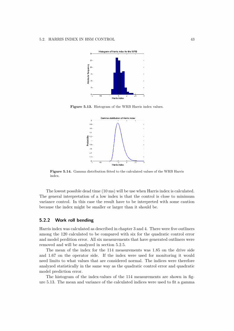
5.2. HARRIS INDEX IN HSM CONTROL 43
Figure 5.13. Histogram of the WRB Harris index values.
Figure 5.14. Gamma distribution fitted to the calculated values of the WRB Harrisindex.
The lowest possible dead time (10 ms) will be use when Harris index is calculated.The general interpretation of a low index is that the control is close to minimumvariance control. In this case the result have to be interpreted with some cautionbecause the index might be smaller or larger than it should be.
5.2.2 Work roll bending
Harris index was calculated as described in chapter 3 and 4. There were five outlinersamong the 120 calculated to be compared with six for the quadratic control errorand model perdition error. All six measurements that have generated outliners wereremoved and will be analyzed in section 5.2.5.
The mean of the index for the 114 measurements was 1.85 on the drive sideand 1.67 on the operator side. If the index were used for monitoring it wouldneed limits to what values that are considered normal. The indices were thereforeanalyzed statistically in the same way as the quadratic control error and quadraticmodel prediction error.
The histogram of the index-values of the 114 measurements are shown in fig-ure 5.13. The mean and variance of the calculated indices were used to fit a gamma
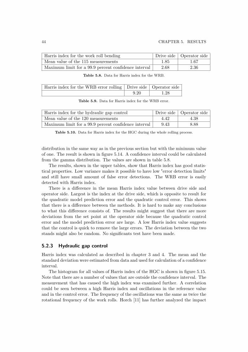
44 CHAPTER 5. RESULTS
Harris index for the work roll bending Drive side Operator sideMean value of the 115 measurements 1.85 1.67Maximum limit for a 99.9 percent confidence interval 2.68 2.36
Table 5.8. Data for Harris index for the WRB.
Harris index for the WRB error rolling Drive side Operator side9.20 1.28
Table 5.9. Data for Harris index for the WRB error.
Harris index for the hydraulic gap control Drive side Operator sideMean value of the 120 measurements 4.42 4.38Maximum limit for a 99.9 percent confidence interval 9.43 8.88
Table 5.10. Data for Harris index for the HGC during the whole rolling process.
distribution in the same way as in the previous section but with the minimum valueof one. The result is shown in figure 5.14. A confidence interval could be calculatedfrom the gamma distribution. The values are shown in table 5.8.
The results, shown in the upper tables, show that Harris index has good statis-tical properties. Low variance makes it possible to have low "error detection limits"and still have small amount of false error detections. The WRB error is easilydetected with Harris index.
There is a difference in the mean Harris index value between drive side andoperator side. Largest is the index at the drive side, which is opposite to result forthe quadratic model prediction error and the quadratic control error. This showsthat there is a difference between the methods. It is hard to make any conclusionsto what this difference consists of. The results might suggest that there are moredeviations from the set point at the operator side because the quadratic controlerror and the model prediction error are large. A low Harris index value suggeststhat the control is quick to remove the large errors. The deviation between the twostands might also be random. No significants test have been made.
5.2.3 Hydraulic gap controlHarris index was calculated as described in chapter 3 and 4. The mean and thestandard deviation were estimated from data and used for calculation of a confidenceinterval.
The histogram for all values of Harris index of the HGC is shown in figure 5.15.Note that there are a number of values that are outside the confidence interval. Themeasurement that has caused the high index was examined further. A correlationcould be seen between a high Harris index and oscillations in the reference valueand in the control error. The frequency of the oscillations was the same as twice therotational frequency of the work rolls. Horch [11] has further analyzed the impact

5.2. HARRIS INDEX IN HSM CONTROL 45
Harris index for the hydraulic gap control Drive side Operator sideMean value of the 120 measurements 1.84 1.86Maximum limit for a 99.9 percent confidence interval 4.31 3.93
Table 5.11. Data for Harris index for the HGC during last pass of rolling.
Figure 5.15. Histogram of all calculated Harris index for the HGC.
Figure 5.16. The reference value for the HGC during the last pass of rolling.
of oscillating control loops on Harris index. His results are in accordance with thosecalculated here. It does not matter that the oscillations were not caused by controlloop oscillations does not matter. Harris index will be high, independent of thereason of the oscillation.
The choice of measurements used for calculations of the different assessment andmonitoring tools was described in the beginning of chapter 5. All 120 measurements
Harris index Small valve leakage Large valve leakage After valve changeWhole rolling 4.44 4.62 4.20Last pass of rolling 1.87 2.02 1.62
Table 5.12. Harris index when the valve leakage changes.

46 CHAPTER 5. RESULTS
Mean 1.8229Standard deviation 0.67436
Table 5.13. Statistical properties for a single index value.
Mean 0Standard deviation 0.15079
Table 5.14. Statistical properties for a difference between a mean of 40 index values.
have been used in the calculations. The measurements were divided in three groups:when the valve leakage is small, when the valve leakage is large and after the changeof valve, when the leakage is very small.
The results can be seen in table 5.12. The index is smaller after the valve change.It becomes larger when the valve leakage is higher.
Significance tests have been made on the changes to verify that they are notrandom variations. The following zero-hypothesis have been chosen.
H0: The difference in index mean values with large valve leakage and after valvechange is zero.
The significance level is chosen to 0.05.The statistical properties of the statistical process have to be estimated under
the condition that H0 is true. The distribution is assumed to be a normal gaussiandistribution to simplify calculations. The mean and standard deviation for a singleHarris index is estimated from the two series of measurements before and after thevalve change. Only measurements from the last pass of rolling is used here. Totally80 values are used for estimation of mean and variance.
A single sample has the distribution N(m,σ). The distribution for the mean of40 samples will be, N(m, σ√
40). The distribution of the difference between two mean
values then becomes, N(0, σ√20
).The difference between the mean before and after the valve change is 0.404.
That corresponds to 2.6792 standard deviations. It can be concluded that this isoutside a 95 percent confidence interval and the zero-hypothesis could be rejected.It was thereby proven that the index has changed after the valve change.
Significance tests have also been made on the change between small and largevalve leakage as well as the changes from the measurements from the whole rolling.These results are enclosed in the appendix.
The results show that the change in index from the whole strip of rolling wasnot significant. The variance is too large and the difference in mean is too small tobe able to make use of the results. The results pointed in the same direction for theindex from the whole rolling as the index from the last stand. It might be possibleto show that the change is significant if another zero-hypothesis is chosen.
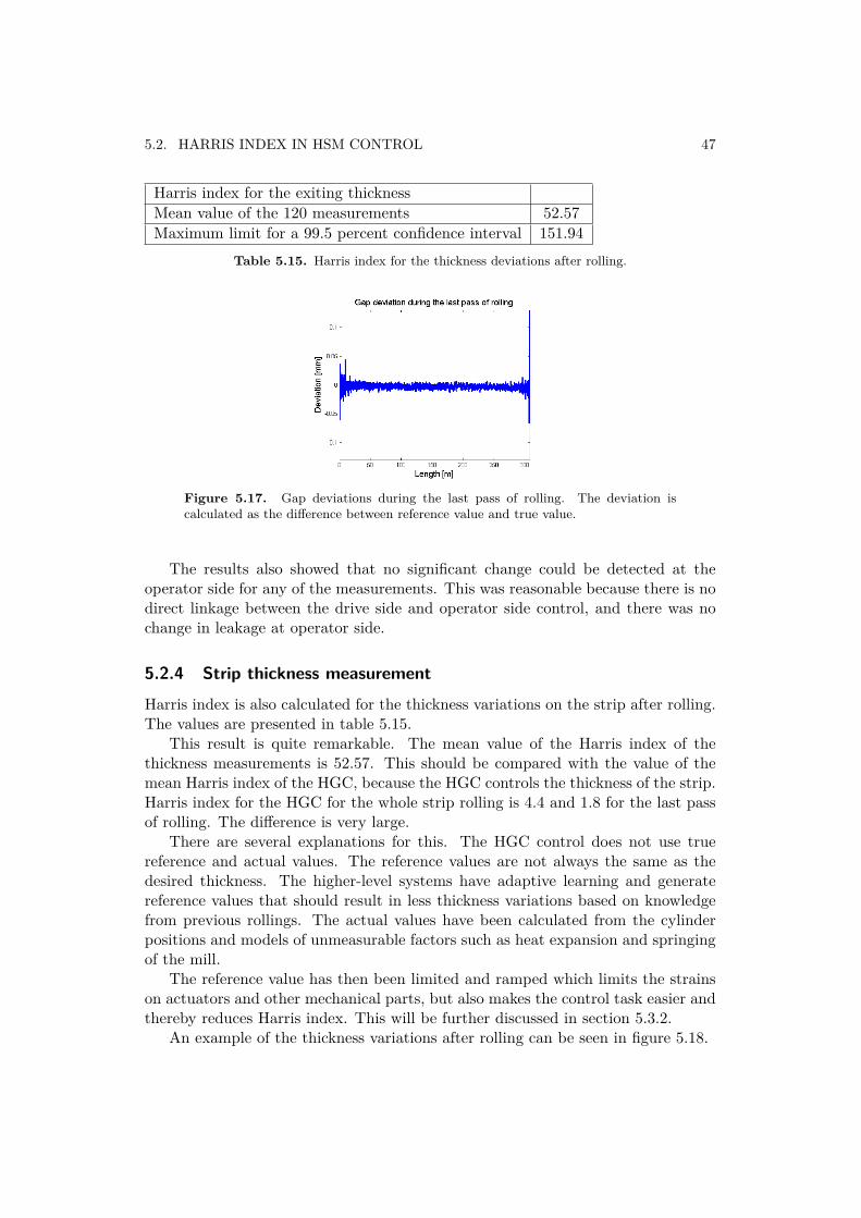
5.2. HARRIS INDEX IN HSM CONTROL 47
Harris index for the exiting thicknessMean value of the 120 measurements 52.57Maximum limit for a 99.5 percent confidence interval 151.94
Table 5.15. Harris index for the thickness deviations after rolling.
Figure 5.17. Gap deviations during the last pass of rolling. The deviation iscalculated as the difference between reference value and true value.
The results also showed that no significant change could be detected at theoperator side for any of the measurements. This was reasonable because there is nodirect linkage between the drive side and operator side control, and there was nochange in leakage at operator side.
5.2.4 Strip thickness measurementHarris index is also calculated for the thickness variations on the strip after rolling.The values are presented in table 5.15.
This result is quite remarkable. The mean value of the Harris index of thethickness measurements is 52.57. This should be compared with the value of themean Harris index of the HGC, because the HGC controls the thickness of the strip.Harris index for the HGC for the whole strip rolling is 4.4 and 1.8 for the last passof rolling. The difference is very large.
There are several explanations for this. The HGC control does not use truereference and actual values. The reference values are not always the same as thedesired thickness. The higher-level systems have adaptive learning and generatereference values that should result in less thickness variations based on knowledgefrom previous rollings. The actual values have been calculated from the cylinderpositions and models of unmeasurable factors such as heat expansion and springingof the mill.
The reference value has then been limited and ramped which limits the strainson actuators and other mechanical parts, but also makes the control task easier andthereby reduces Harris index. This will be further discussed in section 5.3.2.
An example of the thickness variations after rolling can be seen in figure 5.18.

48 CHAPTER 5. RESULTS
Figure 5.18. Thickness deviations on the strip after rolling.
5.2.5 WRB outliners
There are totally six index values calculated from the different methods that aresignificantly different than the other index values calculated for the WRB. Five ofthese appear in all the three different monitoring tools. The control error fromone of these five measurements is shown in figure 5.19. The spikes in the signal arecorrelated with the entering an exiting of the strip in the stand. They are caused bythe sudden change of load and can be viewed as noise in this context. The controlsystem quickly reacts on the control error that the noise has caused and eliminatesit. The contribution from the spikes to the values of the monitoring tools is therebysmall.
A large and long control error is occurring in the end of the signal. It is likelyto have an impact on all the values of the different monitoring tools. The samephenomenon occurs in all five measurements.
Other data saved from these five rollings has shown that the operator abortedthe rolling in all of these five rollings. The ordinary control system is overriddenwhen a rolling is aborted or a stop is made. That is the reason why there is aconstant control error in the end of these rollings. These measurements shouldnever have been chosen if this would have been known in the first place.
Five of the six outliners have been explained. They would not have been aproblem in the real implementation, because the calculation of the values wouldhave been aborted together with the rolling. The last measurement that caused anoutliner did only affect the calculation of the quadratic control error and the modelprediction error, not on Harris index. The control error in the WRB control fromthis measurement is shown in figure 5.20.
A large spike can be seen to the right in figure 5.20. It looks very unphysical andis indeed. The reason is that the values exported and saved by the measurementsystem have a limited amount of resolution and range. The measurements valuestarts all over at the other side of the measurement range if the true signal exceedsthe limits of the range. In this case it is equivalent to a change in force with 4000kN. The signal gets back within the measurement range after one sample.

5.3. ASSESSMENT OF CONTROL LOOPS 49
Figure 5.19. Example of the control error for measurement that has generatesoutliners.
Figure 5.20. Control error from the WRB.
This outliner would not appear if the methods were implemented in the TCS-system or in PPSM because the whole range of the signal is available in the TCS-system.
It is interesting to note that only the quadratic control error method and themodel prediction error method resulted in an outliner. Harris index was withinthe confidence interval. The reason is that although the control error was large itquickly disappeared. This corresponds to a fast controller and thereby a low Harrisindex.
5.3 Assessment of control loops
The ARMAX models used for the model prediction error method have been analysedfurther as suggested in section 4.3. Bode plots and plots of the placement of zerosand poles in the complex plane have been made on both WRB and HGC.

50 CHAPTER 5. RESULTS
Figure 5.21. Bode plot of the closed loop WRB system.
Figure 5.22. Zeros and poles of the closed loop WRB system.
5.3.1 WRB controlThe Bode plot shows that the phase shift between reference and output is small.Note also that amplitude variations in the plot are extremely small. Because thesystem is causal and all its poles are strictly placed inside the unit circle it mustalso be stable. Both the Bode plot and the poles and zero placement indicates thatthe WRB closed loop system is stable at all frequencies.
The calculated Harris indices are very close to one, which suggests that thecontrol is close to minimum variance control. The WRB control has, in contrast tothe HGC, very direct values of the actual and reference values. No models are usedto calculate the actual value. This makes the results more credible.
The reference signal is limited and ramped which makes the index lower thanit should be. Limiting and ramping of the control signal makes the index higher.These two effects contribute to the uncertainty of the true value of the index. Theresults also have to be analyzed with caution because of the low time resolution ofthe measurements.
It is reasonable to say that the control probably is well tuned. Based on theknowledge acquired during the work with this thesis it would be fair to say that thecontrol seems to work satisfactory. Worth to note is that the reference value often

5.3. ASSESSMENT OF CONTROL LOOPS 51
Figure 5.23. Bode plot of the closed loop HGC system.
Figure 5.24. Zeros and poles of the closed loop HGC system.
seems to reach its limit, see figure 1.11. The effects this might have on the stripprofile have not been examined.
5.3.2 HGC controlThe HGC Bode plot and the placement of the zero and poles of the models used inthe model prediction method can be seen in figure 5.23 and figure 5.24.
The Bode plot shows that the phase shift between reference and output aresmall. Because the system is causal and all its poles are strictly placed insidethe unit circle it must also be stable. Both the Bode plot and the poles and zerosplacement indicate that the HGC closed loop system is stable at all frequencies. TheBode plot also show that the gap control has low pass characteristics. This result isin accordance with what is known about the mill and research on the subject [16].The reason for the low pass characteristics is that hydraulic accumulators, cylindersand other parts have low pass properties.
The Harris index calculated for a whole strip rolling is more than twice as largecompared to the WRB. The index gets much smaller when it is only calculated forthe last pass of rolling and is then comparable to the WRB index. An explanationfor this is the system behavior during the contraction of the gap between passes. The

52 CHAPTER 5. RESULTS
reference value is ramped between the passes down to the desired thickness. Thereis a stationary control error during the ramping, which is the most probable cause ofhigh index. This could of course be avoided with a second order integrational partin the control, but it might not be useful. A control error between passes does notaffect the goal of the control. The low index values during the last pass of rollingindicates that the control works well when it needs to.
The Harris index from the HGC is to be considered low but the control doesnot manage to make the thickness variations small in the same extent. The indexfrom the thickness measurement after rolling is almost thirty times as large as theHGC index. There can be several explanations to this large discrepancy.
Limitations in the reference signals can be one explanation. The reference islimited both in the rate of increase and in maximum value. This limits the strainson the mechanical parts but it also makes it impossible to reach the true control ob-jective. This means that the thickness is allowed to deviate from the goal thicknessto avoid damages to the mill.
A second reason for large thickness variations after rolling is insufficient models.Because the true gap between the work rolls, and thereby the thickness of the strip,are not know, it have to be estimated. The cylinder position of the HGC and modelsare used for estimation. There are models for heat expansion in the rolls, springingof the mill, roll wear, and more. If the models are insufficient to describe the millthey will generate actual values that are not the same as the true gap size. Thecontrol will then aim at a gap that is not the same as the desired thickness.
Yet another reason is the physical reality. Large amount of noise and the lackof measurements, sets limits to what are possible to control. Deficiency in sensorscan also be an explanation.
The reason for the high thickness variations after rolling might be a combinationof the reasons suggested above. A closer investigation of this has not been done.
Faster dynamics of the thickness measurment feedback to the reference gener-ation could probebly remove much of the error after rolling. The feedback wouldcompensate for model errors. The risk of makeing the thickness measurment feed-back more faster is that the long deadtime in the feedback might make the systeminstable.
The large difference between the calculated gap and the true thickness measuredcan be seen in figure 5.19 and figure 5.20. The left figure shows the deviation fromthe reference gap. The deviation is very small and there are no stationary deviations.This indicates that the control is working well. The measured thickness in the rightfigure is much different. The thickness deviations is both larger and semi stationary.

5.4. REASONS FOR OSCILLATIONS OTHER THAN OSCILLATING CONTROLLOOPS 53
Number of peak at Number of peak at Number of peak atbackup roll rotation work roll rotation twice the work roll
frequency frequency rotation frequencyStretch signalbefore filter 6 1 9Stretch signalafter filter 0 0 8Thicknessmeasurementafter rolling 4 0 7
Table 5.16.
Figure 5.25. Example of a frequency spectrum of the stretch signal before filtering.A is the backup roll peak, B is the work roll peak, C is the peak at twice the workroll rotational frequency.
5.4 Reasons for oscillations other than oscillating controlloops
5.4.1 Roll eccentricity
Thirteen measurements were used to identify the number of oscillations before andafter the eccentricity filter in the HGC stretch signal.
The measurements were processed as described in the implementation chapter.The result can be seen in table 5.16. Examples of frequency spectra can be seen infigure 5.25 and figure 5.26.
The results show that the eccentricity filter removes the backup roll rotationalfrequency oscillations and the work roll rotational frequency oscillations from thestretch signal. The backup roll rotational frequency appears on the rolled stripanyway. The reason might be that the filter only reduces the effect of eccentricitywithout removing it completely. Another solution to the problem is suggested insection 7.2.
A large number of oscillations at twice the work roll rotational frequency were

54 CHAPTER 5. RESULTS
Figure 5.26. Example of a frequency spectrum of the thickness deviation afterrolling. A is the backup roll peak, B is the work roll peak, C is the peak at twice thework roll rotational frequency.
Figure 5.27. Example of the frequency spectra of the thickness feedback.
detected. The filter only removed one out of nine oscillations. The reason is thatthe filter is not designed to remove oscillations at this frequency. Seven out of theseoscillations were also found on the strip thickness measurements.
It can be concluded that the filter does not remove the effect of eccentricity inrolls. An expansion of the filter to twice the work roll frequency would be an easyway to improve the filtering.
These results are based on thirteen measurements. A larger number of striprollings should be examined to get more reliable results.
5.4.2 Thickness measurement feedback oscillations
The thirteen measurements were processed as described in the implementation chap-ter. The result showed that no one had a frequency peak at the theoretical oscillationfrequency. This result was complemented with visual inspection of the frequencyspectrum of the signals. An example is shown in figure 5.27. There was in fact nofrequency peaks in the frequency spectrum.
This result was not surprising. Oscillations due to thickness measurement feed-

5.4. REASONS FOR OSCILLATIONS OTHER THAN OSCILLATING CONTROLLOOPS 55
back can thereby be ruled out as the cause of oscillations in other parts of thesystem. The detection of backup roll eccentricity is not affected by this feedbackand previous results can be interpreted as suggested.


Chapter 6
Conclusions
This chapter will present the conclusion drawn from the results in the previoussection. Suggestions to what could have been done differently are made.
6.1 Assessment and monitoring tools
The quadratic control error and the quadratic model prediction error monitoringtools works well. They have a narrow distribution around their means, which makesit easy to detect anomalies. Their behavior is stable which enables an implementa-tion.
It is unfortunate that there was only one control error to evaluate the methodson. The methods did however detect rollings where the control had been disabled.
A disadvantage of the two suggested methods is that they do not take goodcontrol into account. Large control errors or deviations from the model will resultin a high index although the control might be optimal. If large noise affects a systemwith a control that quickly eliminates the effect of the noise, it will still lead to largevalues of the index.
The weighted moving average that was suggested in section 4.1.1 did not giveany relevant information that could be used by an operator. It would perhaps bemore interesting to see a weighted moving average of Harris index.
The suggested monitoring tools can be implemented in many different ways. Thewhole rolling process, during the last pass, all passes, during constant reference, andso on. A better choice of the parts of the signals used might make the monitoringtools more reliable.
6.2 Harris index in roll control
The Harris index works well as an assessment tool. The values are narrow dis-tributed around the mean, which make it easy to detect anomalies in a monitoringsituation. Their behavior is stable which enables an implementation.
57
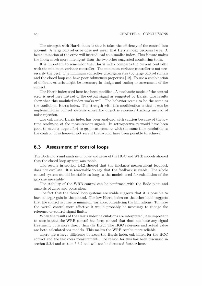
58 CHAPTER 6. CONCLUSIONS
The strength with Harris index is that it takes the efficiency of the control intoaccount. A large control error does not mean that Harris index becomes large. Afast elimination of the error will instead lead to a smaller index. This feature makesthe index much more intelligent than the two other suggested monitoring tools.
It is important to remember that Harris index compares the current controllerwith the minimum variance controller. The minimum variance controller is not nec-essarily the best. The minimum controller often generates too large control signalsand the closed loop can have poor robustness properties [12]. To use a combinationof different criteria might be necessary in design and tuning or assessment of thecontrol.
The Harris index used here has been modified. A stochastic model of the controlerror is used here instead of the output signal as suggested by Harris. The resultsshow that this modified index works well. The behavior seems to be the same asthe traditional Harris index. The strength with this modification is that it can beimplemented in control systems where the object is reference tracking instead ofnoise rejection.
The calculated Harris index has been analyzed with caution because of the lowtime resolution of the measurement signals. In retrospective it would have beengood to make a large effort to get measurements with the same time resolution asthe control. It is however not sure if that would have been possible to achieve.
6.3 Assessment of control loops
The Bode plots and analysis of poles and zeros of the HGC and WRB models showedthat the closed loop system was stable.
The results in section 5.4.2 showed that the thickness measurement feedbackdoes not oscillate. It is reasonable to say that the feedback is stable. The wholecontrol system should be stable as long as the models used for calculation of thegap size are stable.
The stability of the WRB control can be confirmed with the Bode plots andanalysis of zeros and poles alone.
The fact that the closed loop systems are stable suggests that it is possible tohave a larger gain in the control. The low Harris index on the other hand suggeststhat the control is close to minimum variance, considering the limitations. To makethe overall control more effective it would probably be necessary to change thereference or control signal limits.
When the results of the Harris index calculations are interpreted, it is importantto note is that the WRB control has force control that does not have any signaltreatment. It is more direct than the HGC. The HGC reference and actual valueare both calculated via models. This makes the WRB results more reliable.
There are a large difference between the Harris index calculated for the HGCcontrol and the thickness measurement. The reason for this has been discussed insection 5.2.4 and section 5.3.2 and will not be discussed further here.

6.4. REASONS FOR OSCILLATIONS OTHER THAN OSCILLATING LOOPS 59
6.4 Reasons for oscillations other than oscillating loopsFast fourier transforms were used to identify oscillation in the signals. A disad-vantage with this method is that the calculated spectrum has high variance. Thevariance can be reduced with Bartletts or Wechs methods at the cost of less fre-quency resolution. One of these methods would probebly have been better to usein this case.
No thickness measurement feedback oscillations could be found among examinedmeasurement. Visual inspection of the control signal has shown that the gain inthe feedback is small and the dynamics are slow. There is no risk for thicknessmeasurement feedback oscillations.
Oscillations caused by eccentric rolls affect the system. The filters to removethese effects do not remove the oscillations completely especially not the oscillationscaused by elliptic rolls. Because the system do not remove the effect of eccentricitycompletely, it is important to make the rolls as round as possible. It would thereforebe relevant to make roundness measurement at every ground roll in the grindingworkshop.


Chapter 7
Future work
This chapter will give suggestions to future work in research and at the HSM inAvesta. The suggestions are based on the conclusions in the previous section.
7.1 ResearchThe efficiency in the industry has increased every year since the industrial revo-lution. As the industry progress it becomes more and more automated and lesslabor force demanding. With these advances comes a demand on monitoring. Thegoal of the monitoring should be to increase the availability and lower the cost formaintenance and damages to equipment.
This thesis has been made in this context.Werner von Siemens coined the expression "Messen ist Wissen" (measuring is
knowing). Today more than a hundred years later it is maybe about to change,or has already changed. Signal processing becomes more and more essential to"refine" information and make it possible for humans to understand. A key to suc-cesses in the future research is to combine signal processing methods with physicaland mechanical understanding to develop methods for information "refinement" andmonitoring.
Harris index is one of these methods.
7.2 Avesta HSMTo improve the monitoring of the HSM in Avesta it is essential to increase the qualityof information rather then to increase the quantity. Better systems for monitoringof the process could save time for the process engineers, the automation personnelas well as the mechanics.
A better monitoring system could include more advanced signal processing. Itcould also use a several measurements at once when diagnosis of the system is made.
The monitoring system used today measures values and makes some simplesignal treatment and compares the result with limit conditions. The system gives
61
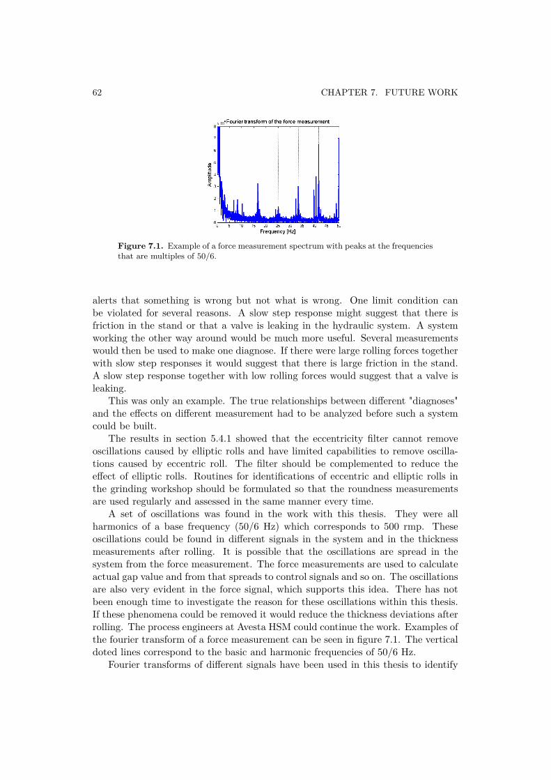
62 CHAPTER 7. FUTURE WORK
Figure 7.1. Example of a force measurement spectrum with peaks at the frequenciesthat are multiples of 50/6.
alerts that something is wrong but not what is wrong. One limit condition canbe violated for several reasons. A slow step response might suggest that there isfriction in the stand or that a valve is leaking in the hydraulic system. A systemworking the other way around would be much more useful. Several measurementswould then be used to make one diagnose. If there were large rolling forces togetherwith slow step responses it would suggest that there is large friction in the stand.A slow step response together with low rolling forces would suggest that a valve isleaking.
This was only an example. The true relationships between different "diagnoses"and the effects on different measurement had to be analyzed before such a systemcould be built.
The results in section 5.4.1 showed that the eccentricity filter cannot removeoscillations caused by elliptic rolls and have limited capabilities to remove oscilla-tions caused by eccentric roll. The filter should be complemented to reduce theeffect of elliptic rolls. Routines for identifications of eccentric and elliptic rolls inthe grinding workshop should be formulated so that the roundness measurementsare used regularly and assessed in the same manner every time.
A set of oscillations was found in the work with this thesis. They were allharmonics of a base frequency (50/6 Hz) which corresponds to 500 rmp. Theseoscillations could be found in different signals in the system and in the thicknessmeasurements after rolling. It is possible that the oscillations are spread in thesystem from the force measurement. The force measurements are used to calculateactual gap value and from that spreads to control signals and so on. The oscillationsare also very evident in the force signal, which supports this idea. There has notbeen enough time to investigate the reason for these oscillations within this thesis.If these phenomena could be removed it would reduce the thickness deviations afterrolling. The process engineers at Avesta HSM could continue the work. Examples ofthe fourier transform of a force measurement can be seen in figure 7.1. The verticaldoted lines correspond to the basic and harmonic frequencies of 50/6 Hz.
Fourier transforms of different signals have been used in this thesis to identify

7.2. AVESTA HSM 63
oscillations. Vibrations can cause oscillations. To use vibrations measurements toanalyze hot strip mills and develop monitoring tools seams to be a very promisingapproach. The following papers published in China Steel Technical Report arerecommended as inspiration in the future work [17], [18] and [19].


Appendix A
Glossary (Ordlista)
English SwedishEngelska Svenska
continues casting plant stränggjutningsanläggningroll valsrolling valsningslabs slabsstrip bandbackup roll stödvalswork roll arbetsvalshot strip mill varmvalsverkcoiler haspelpinch roll looprullarstand valsstolpargrinding slipninghousing valsstolroughing mill förparingots göt, metallstyckesteckel mill steckel verkload cell lastcellfour-high roll stand kvartovalsverk
65


Appendix B
Notation
B.1 Acronyms
s0 gap set points in the gap control∆s gap-size deviation, e.g. caused by stand springingsc gap-size calculated from the cylinder positionsy output variancesMV output variance with minimum variance controly[k] discrete true output signaly[k] discrete output signal estimated by a model∆y[k] discrete model prediction error signale[k] discrete control error signalc[k] discrete control signalu[k] discrete input signale[k] discrete stochastic normal distributed white noiseem[k] model driving discrete stochastic normal distributed white noisefa oscillation frequency of the thickness measurement feedbackfbr backup roll rotational frequencyfwr work roll rotational frequencyDbr backup roll diameterDwr work roll diametervr rolling speedl number of coefficients in an AR-modeld number of sampels of delayhi coefficient in the impulse responseIe quadratic control error indexI∆y quadratic model prediction error indexIH Harris indexme mean estimated from a number of valuesσ2
e noise varianceA(q−1) to L(q−1) parametric time shift series that are used to describe a system
ll
67

68 APPENDIX B. NOTATION
B.2 AbbreviationsHSM Hot Strip MillAGC Automatic Gauge ControlCVC Continously Variable CrownHGC Hydraulic Gap ControlWRB Work Roll BendingPPMS Plant and Process Monitoring SystemHMI Human Machine InterfaceTCS Technological Control SystemPI Proportional IntegratingOS Operator SideDS Drive Side

Appendix C
The hydraulic systems
The mill is equipped with one hydraulic cylinder on each side of the upper backuproll. The cylinders have a maximum cylinder stroke of 110 mm, which is sufficientto make the total reduction of the strip thickness.
The cylinder has a fixed pressure at the rod side at 40 bar. The pressure onthe piston side is controlled by the HGC and is the origin of the rolling force. Thecontrol signal is actuated with a valve. It can be closed, open to a high-pressure sideor open to a low-pressure side, enabling increase or decrease of cylinder pressure.
The high-pressure side has hydraulic pumps that keep the pressure constant at280 bar. It also has accumulators to be able to keep the pressure constant even atlarge flows to the cylinder.
The low-pressure side leads to a tank without any pressure. Filters and checkvalves that leads to the tank keeps the pressure at the low-pressure side to approx-imately 3 bar.
Figure C.1.
69


Appendix D
Significance tests
D.1 Measurements form the last pass of rolling
Drive side Is the change Minimumsignificant (0.05)? significance level
Change between small leakageand large leakage No 0.32Change between large leakageand after valve change Yes 0.008Change between small leakageand after valve change Yes 0.007
Table D.1.
Operator side Is the change Minimumsignificant (0.05)? significance level
Change between small leakageand large leakage No 0.80Change between large leakageand after valve change No 0.72Change between small leakageand after valve change No 0.96
Table D.2.
71

72 APPENDIX D. SIGNIFICANCE TESTS
D.2 Measurements form the whole rolling
Drive side Is the change significant (0.05)?Change between small leakage and large leakage NoChange between large leakage and after valve change NoChange between small leakage and after valve change No
Table D.3.
Operator side Is the change significant (0.05)?Change between small leakage and large leakage NoChange between large leakage and after valve change NoChange between small leakage and after valve change No
Table D.4.
Bibliography
[1] Varmvalsverk, Jernkontoret, Norstedts Tryckeri AB, Stockholm 1997, Sweden,ISBN 91-971474-8-6
[2] A.I. Tselikov, G.S. Nikitin, S.E. Rokotyan, The theory of lengthwise rolling,Mir Publishers, 1981
[3] Lathund för examensarbeten vid S3, 23:ed August 2005,http://www.s3.kth.se/signal/edu/exjobb/rules.pdf
[4] K.B. Goode, B.J. Roylance, J. Moore, Development of model to predict condi-tion monitoring interval times, Ironmaking and steelmaking 2000 Vol. 27 No.1
[5] A. P. Swanda, D. E. Seborg, Control performance Assessment Based on Set-point Response Data, Proceedings of the American Control Conference, SanDiego California 1999
[6] D. B. Ender, Process Control Performance: Not as Good as you Think, ControlEngineering., vol. 40, no. 10, 1993
[7] T. Harris, Assessment of control loop performance, The Canadian Journal OfChemical Engeneering 67", 856-861
[8] C. B. Lynch, G.A. Dumount, Control Loop Performance Monitoring, Sec-ond IEEE Conference on Control Applications, 835-840, Vancouver Canada,September 1993
[9] T. Glad, L. Ljung, Reglerteknik Grundläggande teori, Andra upplagan, Stu-dentlitteratur, Lund 1989.
[10] L. Ljung, T. Glad, Modellbygge och simulering, Studentlitteratur, Lund 2004,ISBN 91-44-02443-6
[11] A. Horch, Condition Monitoring of Control Loops, Doctoral Thesis, KTH,Stockholm 2000, ISBN 91-7170-638-0
[12] P-G. Eriksson, A. J. Isaksson, Some Aspects of Control Loop PerformanceMonitoring, The 3rd IEEE Conference on Control Applications, Glasgow 1994,Scotland, 1029-1034
73
74 BIBLIOGRAPHY
[13] B-S. Ko, T. F. Edgar, Assessment of Achievable PI Control Performance forLinear Processes with Dead Time, Proceedings of the American Control Con-ference, Philadelphia 1998, vol.3,1548-1552
[14] L. Ljung, System Identification - Theory for the user, Second edition, Prentice-Hall PTR, New Jersey 1999, ISBN 0-13-656695-2
[15] A. J. Isaksson, A. Horch, G.A. Doumont, Event-triggered deadtime estimation- comparison of methods, American Control Conference, 2001, vol.4 , 3280 -3285
[16] R-M Guo, Evaluation of dynamic characteristics of HAGC system, Iron andSteel, July 1991, 52-61
[17] J-J Jeng, C-Y Wei, K-M Chang, Case Studies of the On-Line Monitoring andDiagnostic System for Machinery of the CSC No.2 Hot Strip Mill, China SteelThechnical Report, No. 13, 1999, 93-101
[18] J-J Jeng, Condition Diagnostic Rules for Hot Strip Mill Pinch Rolls UsingVibration Signals, China Steel Technical Report, No. 15, 2001, 59-69
[19] J-J Jeng, C-Y Wei, H-M Liu, Development of On-Line Chattering Monitoringand Diagnosis System for Stainless Steel Hot Strip Mills, China Steel TechnicalReport, No. 18, 2004, 30-37