Looking for Someone to Blame:

Delegation, Cognitive Dissonance, and the

Disposition Effect∗

Tom ChangUniversity of Southern California

David H. SolomonUniversity of Southern California

Mark M. WesterfieldUniversity of Washington

April 2014

Abstract

We analyze brokerage data and an experiment to test a cognitive-dissonance basedtheory of trading: investors avoid realizing losses because they dislike admitting thatpast purchases were mistakes, but delegation reverses this effect by allowing the investorto blame the manager instead. Using individual trading data, we show that the disposi-tion effect – the propensity to realize past gains more than past losses – applies only tonon-delegated assets like individual stocks; delegated assets, like mutual funds, exhibita robust reverse-disposition effect. In an experiment, we show increasing investors’ cog-nitive dissonance results in both a larger disposition effect in stocks and also a largerreverse-disposition effect in funds. Additionally, increasing the salience of delegationincreases the reverse-disposition effect in funds. Cognitive dissonance provides a unifiedexplanation for apparently contradictory investor behavior across asset classes and hasimplications for personal investment decisions, mutual-fund management, and interme-diation.

∗Contact at tychang@marshall.usc.edu, dhsolomo@marshall.usc.edu, and mwesterf@uw.edu respectively.We would like to thank Nick Barberis, Zahi Ben-David, Ekaterina Chernobai, Bill Christie, Harry DeAngelo,Wayne Ferson, Cary Frydman, Mark Grinblatt, Jarrad Harford, David Hirshleifer, Markku Kaustia, KevinMurphy, Ed Rice, Antoinette Schoar and seminar and conference participants at the Behavioral EconomicsAnnual Meeting, CCFC, WFA, Cal Poly Pomona, Emory, Northwestern University, Notre Dame, UC Berke-ley, UCSB, UCSD Rady, Universtiy of Oregon, University of Washington, University of Wisconsin Madison,and USC for helpful comments and suggestions. We especially thank Terry Odean for sharing the individualtrading data.

1 Introduction

In recent years, economists have come to appreciate the importance of household investment

decisions for understanding both decision making under risk and the behavior of investors in

financial markets (e.g. Campbell (2006)). One of the most robust facts describing individual

trading behavior is the disposition effect: investors have a greater propensity to sell assets

when they are at a gain than when they are at a loss.1 Despite the near-ubiquity of the

disposition effect, the underlying mechanism is not well understood. Empirical work has

been much more successful in identifying problems with various proposed explanations than

in finding positive evidence that points directly to a particular theory to the exclusion of

all others.2

In an apparently puzzling contrast, the disposition effect is reversed in mutual funds, as

investors have a greater propensity to sell losing funds compared to winning funds. This fact

has been known at least since Friend et al. (1970), but it has primarily been discussed in the

context of the positive performance/flow relationship (e.g. Chevalier and Ellison (1997)):

funds that exhibit high returns receive greater inflows, while those with low returns receive

outflows. Importantly, the finding holds for flows from existing investors as well as new

investors (Ivkovic and Weisbenner (2009) and Calvet et al. (2009)). With a few exceptions

(e.g. Kaustia (2010a)), the positive performance/flow relationship has not been thought

of as equivalent to a reverse disposition effect, and it has received little discussion in the

literature that seeks to understand what causes the disposition effect.

In this paper, we examine cognitive dissonance as a parsimonious model for understand-

ing variation in the disposition effect both within and across asset classes. We begin by

1Across asset markets, the disposition effect has been documented in stocks (Odean (1998)), executivestock options (Heath et al. (1999)), real estate (Genesove and Mayer (2001)), and on-line betting (Hartzmarkand Solomon (2012)). Across investor types it has been found in futures traders (Locke and Mann (2005)),mutual fund managers (Frazzini (2006)), and individual investors (for the US Odean (1998), for FinlandGrinblatt and Keloharju (2001), and for China Feng and Seasholes (2005)).

2See the discussion in Section 5.

1

describing the psychological theory of cognitive dissonance – formalized by a three-period

trading model in the appendix – and demonstrating how cognitive dissonance can generate

a disposition effect in non-delegated assets stocks but a reverse disposition effect in dele-

gated assets like mutual funds. We then analyze data from individual trading accounts and

an experiment in order to provide positive evidence in favor of cognitive dissonance as a

driver of the disposition effect. We also show that several broad classes of existing theories

– such as rational and semi-rational learning models, purely returns-based preferences, and

variation in risk attitudes – are insufficient to explain our results. Finally we provide di-

rect empirical evidence of the role of cognitive dissonance in generating a disposition (and

reverse disposition) effect from an online trading experiment.

Cognitive dissonance is defined as the discomfort that arises when a person recognizes

that he or she makes choices and/or holds beliefs that are inconsistent with each other

(Festinger (1957)). We argue that investors feel a cognitive dissonance discomfort when

faced with losses – there is a disconnect between the belief that the investor makes good

decisions and the fact that the investor has now lost money on the position. While all

losses cause such dissonance, realized losses create a greater level of discomfort than paper

losses: because when the loss exists only on paper the investor is able to partly resolve the

dissonance by convincing themselves that the loss is only a temporary setback. This reduces

the blow to their self-image of being someone who makes good decisions. When the loss is

realized, however, it becomes permanent which makes it harder for the investor to avoid the

view that buying the share may have been a mistake. Cognitive dissonance thus provides

the basis for an overall reluctance to realize losses, thus generating a wedge relative to the

investor’s propensity to realize gains (where no such dissonance discomfort exists).

Importantly, however, in the case of delegated assets where decision-making authority

has been ceded to an outside agent, investors can instead resolve the disutility of realized

losses by scapegoating and blaming the manager. Specifically, if the asset is delegated,

2

then the investor can blame/punish the fund manager for the poor performance and sell

the asset – making the loss permanent – without admitting to his or her own mistakes. At

its simplest level, the model captures the intuition that investors do not like to admit that

they were wrong, and will blame someone else if they can.3

Our first main contribution is to empirically document the scope of the puzzle: how

much does the disposition effect vary across asset classes? In individual trading data (the

dataset used in Barber and Odean (2000)), we show that the disposition effect in stocks

and the reverse-disposition effect in actively managed funds holds for the same investors at

the same time. In contrast, investors in passively managed funds (e.g. index funds), where

the role of the portfolio manager is minimal, exhibit a small but directionally positive

disposition effect that is significantly different from actively managed funds but not from

stocks. Looking across a broad range of asset classes (including options, warrants, bond

funds, real estate trusts, etc.), we find the level of the disposition effect is almost rank-

ordered with delegation, and the effect of delegation survives controlling for other asset

class characteristics such as volatility, holding period, and position size. In addition, the

variation across asset classes is driven by differences in the propensity to sell losses, which

is consistent with the effects of cognitive dissonance which is primarily a theory about how

investors react in the loss domain.

The existing literature focuses on understanding the disposition effect in general, but

it does not provide a ready explanation for the variation across asset classes. Because the

variation in trading behavior across asset classes exists even within investors that hold both

assets, the variation is unlikely to be due to clientele-based explanations, such as investors

in each asset class having different preferences over returns or risk. If the disposition effect

3See Barberis (2011) for a discussion of cognitive dissonance in the context of bank losses during thefinancial crisis. The idea that delegation is useful because it provides someone to blame for poor performancesimilar in spirit to an idea in Lakonishok et al. (1992). In their analysis of delegated portfolio managementof tax-exempt funds, the authors state that part of the appeal of external management of pension fundsis the result of a desire by the treasurer’s office “to delegate money management in order to reduce itsresponsibility for potentially poor performance of the plan’s assets”

3

is driven purely by preferences over returns (e.g. prospect theory, realization utility), some

other factor must be invoked to explain its nonexistence in funds. Finally, our trading-

data results motivate a direct experimental test of the role of delegation where we can

exogenously increase the psychological impact of delegation and cognitive dissonance on an

individual’s choices, while holding fixed the economic differences in the underlying assets

and managerial skill.

Our second main contribution is to provide direct, positive evidence of the role of cogni-

tive dissonance in generating the disposition effect. We run an online trading experiment in

which undergraduate students trade a preselected group of actual stocks or funds at daily

market closing prices over a period of 12 weeks. Participants were subjected to two different

randomized treatments. All students had to give a reason for purchasing an asset (stock

or fund), and the first treatment, which we call the “Story” treatment, reminds students

of their stated reason when they move to sell the asset. By emphasizing their previous

choice and its reasons, this treatment is designed to increase the cognitive dissonance dis-

comfort that students experience when facing a loss, and therefore to increase the actions

that individuals will take in response to the cognitive dissonance.

As predicted, we find that this treatment generates an increase both in the magnitude

of the disposition effect for stocks and also the magnitude of the reverse-disposition effect

for funds. The fact that the same treatment has opposite effects for stocks and funds is

consistent with the effect of cognitive dissonance (as both actions are hypothesized to be

responses to the same underlying cognitive dissonance discomfort). It is, however, difficult

to reconcile with competing explanations, particularly since students are not provided with

any information other than their own previously stated reasons for their purchases.

The second treatment, which we call the “Fire” treatment, is designed to increase the

salience of the intermediary (i.e. the fund manager) while preserving all the underlying eco-

nomic differences that may be associated with delegation. Students in the Fire treatment

4

have the words “Buy”, “Sell”, and “Portfolio performance/gain/loss” replaced with the

words “Hire”, “Fire”, and “Fund Manager’s performance/gain/loss” throughout the web-

site. In addition, students in the Fire treatment are provided with links to fund managers’

biographies. As predicted, when the role of the manager is made more salient to investors,

they display a larger reverse-disposition effect.

Finally, we report the results of a survey conducted at the conclusion of the experiment

to examine the impact of our treatments on investor learning. One potential concern is that

increasing the salience of fund managers increases learning with regards to fund manager

skill. We use the survey results to test this possibility directly. We find that while the

treatments themselves have no impact on self-reported measures of learning, the mean

effect masks an asymmetry as predicted by cognitive dissonance: individuals report more

learning conditional on having an aggregate gain than an aggregate loss.4

Our results suggest that cognitive dissonance is an important driver of the disposition

effect, and that the psychological effects of portfolio delegation help explain the apparently

contradictory household behavior across different asset classes. These conclusions suggest

a reinterpretation of some of the existing theories of the disposition effect. Models based

on prospect theory or realization utility have primarily contemplated investors as having

preferences over the returns themselves. Instead, our findings suggest that at least part of

the carrier of utility when evaluating portfolio gains and losses is the psychological costs of

admitting mistakes and resolving cognitive dissonance.

In addition, our results have implications for mutual fund management and intermedi-

ation. Because the disposition effect measures households’ propensity to withdraw funds

after a gain relative to a loss, it also measures the financial slack available to intermediaries

from the household sector after price declines. Instruments that are passive or that give

4Cognitive dissonance predicts that learning should be asymmetric in gains and losses, as shown in othersettings (e.g. Kuhnen (2013) and Mobius et al. (2012)). The asymmetry arises from the fact that individualsare more likely to discount new information if it suggests that the decision to purchase the asset was a badone.

5

households a greater sense of “ownership” in investment decisions may have less fragility in

their funding during crises. We discuss these implications in section 5.4 and point to areas

of potential future research.

2 The Intuition Behind Cognitive Dissonance

In this section we introduce cognitive dissonance intuitively. The theory is formalized in a

simple model in Appendix A.

Social psychology defines a “cognition” as a mental process or thought and “dissonance”

as the conflict created when an individual simultaneously holds two contrary or dissonant

cognitions. Cognitive dissonance theory, which has been characterized as “the most impor-

tant development in social psychology” (Aronson (1997)), holds that when one experiences

such dissonance, it creates an unpleasant feeling that one will go to great lengths to alleviate.

Individuals can then reduce the dissonance in one of three ways:

1. Changing one or both cognitions so they are congruent.

2. Altering the importance of one of the cognitions.

3. Adding a third, ameliorating cognition.

The first mechanism is the one most familiar to economists and is utilized in rational learning

models (e.g. Bayesian updating of one’s priors). For example, if I believe that I am a skilled

investor and receive information that my portfolio has declined in value, I can reduce the

dissonance between these two contradictory cognitions by updating my belief about my skill

level and reducing my estimate of my ability, such as in Seru et al. (2009).

While economists have traditionally focused on this mechanism – assuming individuals

dispassionately incorporate new information to update their beliefs about the world – the

psychological evidence is that new information contradicting one’s priors is often met with

6

a combination of defense mechanisms and mental tricks. One of the key findings in this

literature is the important role of actions in shaping beliefs. Once an action is undertaken in

support of a belief, since individuals believe that their actions are done for good reason, this

belief becomes extremely strong. So strong that if “he is presented with unequivocal and

undeniable evidence, that is belief is wrong... The individual will frequently emerge, not only

unshaken, but even more convinced of the truth of his beliefs than ever before.”5. That is,

when faced with a subsequent cognition dissonant with the original decision-consistent one,

individuals will use various psychological means to reduce dissonance-related discomfort

without relinquishing the original cognition.6

There is a direct map between the three methods for reducing dissonance and whether

or not investors will display a disposition effect. The two relevant cognitions after an asset

has declined in value are:

1. The original decision-identity cognition: “I bought this stock/fund for a good reason.”

2. The new information that the stock or fund went down in value.

Notice that there is no dissonance when the stock or fund increases in value. Nonetheless,

since the disposition effect only describes the difference between the willingness to sell at a

gain versus a loss, an effect that operates only in the loss domain is sufficient to generate

the observed patterns.

The first way of dealing with cognitive dissonance is to change one or both cognitions so

they are congruent. Given that the new information (i.e. the asset has decreased in value)

5Festinger (1957)

6Once a decision has been made, individuals will tend to change their future actions and beliefs tojustify the decision, rather than question the rationale behind the initial decision. Examples include inducedcompliance (e.g. Festinger and Carlsmith (1959) and Aronson and Carlsmith (1963) among many others),the free choice paradigm (e.g. Brehm (1963) and Egan et al. (2010)), effort-justification (Aronson and Mills(1959)), belief disconfirmation (Festinger et al. (1956)), and the Benjamin Franklin effect (Jecker and Landy(1969)). More generally, arguably the key finding in the literature on self-concept or self-identity is thatfacts and preferences are molded to fit one’s identity, as opposed to the other way around.

7

is generally hard to interpret in a positive fashion, this would entail changing the original,

decision-consistent cognition – that is, relinquishing the notion that buying the asset was

a good idea. Traders resist this path because the action-supported cognition is extremely

stable and difficult to change.

The second way of dealing with dissonance is to alter the importance of one of the

cognitions. Because actions create particularly strong links between cognition and identity,

it is difficult to reduce the perceived importance of the initial purchase decision. Instead,

it is easier to convince oneself that the new information in the price decline is unimportant

or irrelevant. For example, investors may prefer to rationalize their poor performance as a

temporary setback due to bad luck or noise in stock returns.

The third way of dealing with dissonance is to introduce an ameliorating cognition.

When the asset is a delegated portfolio, such a cognition is readily available: the decline

can be blamed on the portfolio manager. The portfolio manager is particularly salient for

blame attribution and punishment because he or she has several key characteristics. First,

the fund manager has a clear impact on returns. Second, the task of the portfolio manager

(picking assets with high returns) is very similar to the task of the investor. Finally, the fund

manager has been chosen by the investor themselves specifically for the task of generating

good returns.7 In contrast, index fund managers and CEOs are examples of agents for

which this scapegoating would be less common because both types of agents have specific

jobs that are not similar to the investor’s own decision (matching an index or running a

company), the index fund manager does not determine returns, and the CEO is not chosen

by the (small, household) investor.

7Bartling and Fischbacher (2012) show that “responsibility attribution can be effectively shifted [to adelegate], and ... this can constitute a strong motive for the delegation of a decision right.” In addition,they document blame attribution as a function of the ability to influence returns. Gurdal et al. (2013) showexperimentally that participants blame delegates even when the delegate had no ability to actually influenceoutcomes. They explain this with a theory of “salient perturbations” (from e.g. Myerson (1991), a salientperturbation of a game is another game that is “very similar (in some sense).”) and by noting the similarityof their experimental setup to a more standard principal-agent setup.

8

By blaming the manager, investors can sell losing funds without having to face the

psychological cost of having made a poor decision. Logically, investors could (and maybe

should) still choose to blame themselves for their role in the returns if they wished – nonethe-

less, the point of cognitive dissonance theory is that they are looking for a reason to excuse

their own behavior, so having such a reason at hand makes it likely that investors will

choose that course instead.

In sum, the fact of a loss creates a psychological pain that the investor seeks to resolve.

Regardless of what path the trader takes to resolve cognitive dissonance, realizing losses

has an impact above and beyond the financial consequences, as with Barberis and Xiong

(2009, 2012). While selling itself does not generate new information, it makes the status

of the existing gain/loss ‘permanent’ and confirms a particular narrative episode (e.g. I

bought share X at $10 and sold it at $5). One method of resolving cognitive dissonance is

to downplay the information, and take the appropriate inaction. This effect generates an

overall reluctance to realize losses relative to gains, thereby creating a positive disposition

effect. For delegated assets, a second method is to blame and punish a scapegoat (the

manager). Since punishing the manager by selling reduces the pain associated with cognitive

dissonance, our investor will have a higher propensity to sell loser funds than winner funds

(a negative or reverse disposition effect), and not just a reduced but positive disposition

effect.

Our hypothesis is that when a manager is available, scapegoating is the easiest way to

resolve cognitive dissonance, and therefore investors will sell actively managed funds after

losses more than after gains. When a manager is not available, the second method is easiest

and investors will sell stocks after gains more than after losses. We formalize this logic in a

three-period model in Appendix A. We predict that:

1. Assets that are delegated portfolios will display a reverse-disposition effect, while those

that are not delegated will display a disposition effect. This difference is due to the

9

psychological effects of delegation rather than the economic effects.

2. If investors have a higher level of cognitive dissonance, they will display a larger

disposition effect in non-delegated assets like stocks and a larger reverse-disposition

effect in delegated assets like funds. Similarly investors with low levels of cognitive

dissonance will display little to no disposition effect.

3. If investors focus more on the role of the fund manager instead of their own role, they

will display a larger reverse-disposition effect.

3 Evidence from Small Investor Trading Data

We begin by examining the extent to which real world trading data are consistent with

cognitive dissonance and other explanations of the disposition effect. Data from individual

trading is most suited to testing the first of the predictions above, namely whether delegated

assets have more of a reverse-disposition effect than non-delegated assets. We document

three new stylized facts based on the Barber and Odean (2000) small-investor trading data:

• The disposition effect in stocks and the reverse-disposition effect in funds are shown

by the same investors at the same time (Table II).

• Across asset classes, investor-chosen assets are associated with a positive disposition

effect and delegated-portfolio assets are associated with a reverse disposition effect

(Table III).

• Within equity mutual funds, index funds (which have a fund manager, but one who

plays a less important role in terms of delegated management) display a small positive

and statistically insignificant disposition effect. This effect is significantly different

from other mutual funds but not from stocks (Table IV).

10

Our results are robust to several robustness tests and extensions, including alternate con-

trols, samples, weighting schemes, and combinations of fixed effects, as described in Section

3.5 and detailed in Appendix B.

3.1 Data

The individual trader data used are the same as in Barber and Odean (2000). The data

come from a large discount brokerage and include 128,829 accounts with monthly position

information, comprising 73,558 households (out of 78,000 initially sampled), from January

1991 to November 1996. The data comprise a file of monthly position information and

a file of trades. For each position in an individual’s portfolio, we use the information

on purchases in the trades file to calculate the volume-weighted average purchase price

(“purchase price”) for each point in time. If a position is eliminated entirely and later

repurchased, the purchase price is reset to zero upon the sale of the entire position. Assets

are excluded from the analysis if they were held during the first month of the sample since

this implies they were purchased at an unknown price before the start of the sample.

Once the purchase price is known for each security, we compare the gains and losses

investors face on each security at the end of each month using the positions file. To obtain

a snapshot of securities prices at each point in time from which to calculate gains and

losses, we rely on the prices and holdings in the monthly position files.8 Using the portfolio

snapshot each month, we match each security in the portfolio with the most recent purchase

price. By comparing the price with the purchase price, we define the variable Gain to be

equal to one if the price is greater than the purchase price and zero otherwise.

We then classify each position according to the change in the individual’s position be-

tween the current month and the next month. The variable Sale equals one if the individual

8We do this to ensure that all assets are using comparable price information at the same point in time.Daily price information is not available during the sample period for many of the asset classes that we areinterested in (e.g. mutual funds, preferred stocks, options).

11

reduced the size of their position between the current month and the next month and zero

otherwise. Similar to Odean (1998), we examine the portfolio of gains and losses on all dates

when an individual investor conducted a sale of any security in their account. In periods

where there is no sale at all, it is difficult to tell if this is a deliberate choice by the investor

or simple inattention. By comparing only months with sales, we ensure that the investor is

actually paying attention to their portfolio during that period. Table I presents summary

statistics for the individual trader data.

3.2 The Disposition and Reverse-Disposition Effects

In the main analysis, we test whether individuals exhibit a higher tendency to sell those

securities that are at a gain than those that are at a loss. To do this, we use the following

as our basic regression specifications:

Saleijt = α+ βGainijt + εijt, (1)

Saleijt = α+ βGainijt + γGainijt × Fundj + δFundj + εijt, (2)

where (1) is estimated separately on stocks and funds and (2) is run on the combined data.

Observations are at the account (i), asset (j), and date (t) level, and they are included for

all stocks or funds (according to the specification) on months where the investor sold some

position in their overall portfolio. In addition, as described above, Sale is a dummy variable

equal to one if the individual reduced their position in the asset in that month and zero

otherwise, and Gain is a dummy variable that equals one if the asset was at a gain at the

start of the month and zero otherwise. Fund is a dummy variable equal to 0 for stocks and

1 for funds. In all our regressions, standard errors are two-way clustered at the account and

date levels.

Because the dependent variable is a dummy variable equal to one if the asset was sold, the

mean of the dependent variable is the probability of selling a particular position given that

12

the investor sold something that day. By regressing this variable on Gain, the constant in

the regression measures the probability of selling a position that is at a loss (i.e. Gain=0).

The coefficient on Gain measures the increase in the probability of selling a position if

that position is at a gain, and this coefficient is the measure of the disposition effect –

the increased propensity to sell gains relative to losses.9 A negative coefficient indicates a

reverse-disposition effect.

The purpose in running the two regression specifications is to separately test whether

the disposition effect in stocks and funds are different from zero and from each other.

The coefficient on Fund×Gain in (2) measures the difference in the disposition effect for

stocks and funds. Here, β represents the disposition effect (i.e. the difference between the

propensity to sell gains vs. losses) for stocks, and the sum of the two coefficients β and γ

provides a measure of the disposition effect for funds.

To determine if the difference in the level of the disposition effect in stocks and funds is

driven by a clientele effect – selection of different investor types into each asset class – we

test the disposition effect across various subsets of investors and assets. We examine: 1) all

investors in each asset class; 2) investors who held both stocks and funds at some point in

their trading history, considering all observations from both asset classes; 3) investors who

held both stocks and funds at the same time, considering only observations in the months

where they hold both assets simultaneously. Group 3 is the most stringent test since this

involves a single investor reacting to the returns of stocks and funds at the same time,

allowing us to measure an individual’s concurrent disposition effect across the two asset

classes.

The results of these regressions are presented in Table II. We observe the presence of

9The regression specification in (1) is also analogous to the method used in Odean (1998), who calculatesthe disposition effect as the difference between the proportion of gains realized (PGR) and the proportionof losses realized (PLR). In the regression above, the probabilities will be the same as the proportions, andthe coefficient on Gain is the difference between PGR and PLR. The main advantage of using a regressionspecification is that additional controls can be added in later tables, and the standard errors can be clusteredproperly to avoid assuming that every sale choice is entirely independent.

13

a significant disposition effect in stocks and a significant reverse-disposition effect in funds,

even within the set of investors who simultaneously hold both assets. For all investor subsets,

the coefficient for Gain is positive for stocks and negative for funds (with all coefficients

being significant at the 5% level or greater).

The Gain coefficient for the stock-only sample ranges from 0.0391 for the all-investor

sample to 0.0157 for the investors who simultaneously hold both stock and funds. The

interpretation of this coefficient is that in months when an investor sells some asset, they

are between 3.91% and 1.57% more likely to sell a stock if it is at a gain. This is compared

with the base probability of selling any stock (from the constant in the regression), which is

21.7% for all investors and 18.9% for those simultaneously holding both stocks and equity

mutual funds.

For equity mutual funds, the coefficient for Gain ranges from -0.0656 for the all-investor

sample to -0.0485 for investors who simultaneously hold both stocks and equity mutual

funds, again significant at the 5% level or greater. Investors are between 6.56% and 4.85%

less likely to sell a fund if it is at a gain, compared with the base probability of selling

any fund (on months with the sale of some asset) of 32.5% and 23.2%. In addition, the

Fund×Gain coefficient is negative and significant at the 1% level in all cases.

Note also that the difference in the disposition effect between stocks and funds is driven

by differences in investor propensity to sell losses. The coefficient for Fund, which measures

the differential propensity to sell funds at a loss compared with stocks at a loss, is large and

significant. By contrast, the sum of the coefficients for Fund and Fund×Gain, which mea-

sures the propensity to sell funds at a gain versus stocks at a gain, is small and statistically

insignificant in all three investor groups.

The fact that the Gain coefficient (for both stocks and funds) gets somewhat closer

to zero as the sample gets more restricted suggests that there are some differences be-

tween stock and fund investors that affect the level of the disposition effect being displayed.

14

Nonetheless, the fact that the difference between stocks and funds holds for the same set of

investors at the same time means that differences between investors, such as preferences or

information, cannot explain all of the difference in investor behavior.

These results are difficult to reconcile with theories that posit that the disposition effect

is purely the result of selection into assets according to differences in investor preferences

over returns. Instead, it appears as though there is something about the asset classes

themselves that is driving the difference in the sign of the disposition effect between stocks

and funds.

3.3 Delegation and the Disposition Effect Across Asset Classes

One key feature of our cognitive dissonance-based predictions is the important role inter-

mediaries can play in resolving cognitive dissonance. If delegation is the relevant asset

class characteristic, then delegation provides a testable prediction across a range of asset

classes other than equities and equity mutual funds: if the asset involves delegated portfolio

management, it ought to have a reverse-disposition effect, and if it does not, it ought to

have a disposition effect. By contrast, if the reverse-disposition effect is limited to equity

mutual funds, this would suggest that the distinction may be more likely due to some other

institutional features of such funds.

We test whether delegation is the relevant characteristic by re-running the regression (1)

separately for each asset class label reported in the data. While some of the labels describe

similar types of assets (e.g. various types of equity mutual funds), for transparency we

report separately each of the classifications listed by the trading firm. These classifications

include warrants, options, convertible preferred stock, bond mutual funds, and others. The

only asset class we exclude is money market funds; many of these have a price that is fixed

at some value such as one dollar per share, and hence there are very few observable gains

15

and losses.10

Table III lists the different fund asset classes, an indicator for whether or not they

are delegated, and the coefficient on Gain from (1) estimated using only that asset class.

These asset classes, ordered in terms of their disposition effect, show a striking relationship

between the level of the disposition effect and delegation: while investors usually exhibit a

positive disposition effect for un-managed assets like stocks, actively managed asset classes

usually exhibit a reverse-disposition effect. Of the 24 different asset classes reported by

the trading firm, all 4 asset classes with statistically significant positive disposition effects

are non-delegated portfolios. Of the 7 assets with statistically significant reverse-disposition

effects, 5 are actively managed, with the two exceptions (preferred stock and options equity)

accounting for the two smallest (in magnitude) coefficients.

3.4 Index Funds

In examining the role of delegation, index funds are a useful test case because while they

have many of the same institutional details as actively managed mutual funds, the fund

manager does not actively trade the underlying securities. It seems likely that investors do

not think that index funds will generate abnormal returns; indeed, the whole rationale for

passive investing is that it is pointless to attempt to generate abnormal returns and beat

the market. Thus, the fund manager of an index fund is a less credible target to blame for

the poor performance of the fund, and we expect that – despite all the institutional and

return-moment-based similarity with mutual funds – index funds will not exhibit a reverse-

disposition effect. In addition, since an investment in index funds is often in support of a

10For each asset class, we also attempt to classify them according to whether the asset involves delegationto a portfolio manager. There are some cases where this distinction is not entirely clear. In the case of aReal Estate Trust, where the assets are fixed over long periods, it is not easy to say whether the managerhas more in common with the CEO of a regular industrial company or a portfolio manager of a fund. Weclassify Real Estate Trusts as delegated, interpreting the ambiguity conservatively in the way that will workagainst the main relationship. A similar question arises for Master Limited Partnerships; we classify theseas being non-delegated, although the estimated disposition effect is close to zero and also close to the middleof the asset class range, and hence changing the classification does not significantly affect the results.

16

passive strategy, we expect that index funds will display less of a positive disposition than

stocks.

To test this prediction, we take the names of mutual funds from the CRSP Mutual

Funds database and classify funds as an index fund if their name contains any of ‘Index’,

‘S&P 500’, ‘Russell 2000’, ‘Dow 30’, or variations thereof. We match these classifications

with the trader database using the CUSIP of the funds. The CUSIP data for the CRSP

database only become available starting in 1996. We use CUSIPs between 1996 and 2001

and merge these with CRSP data from earlier years. In addition to the basic regression of

Sale on Gain for index funds, we also run the following regression:

Saleijt = α+ βGainijt + γGainijt × Indexj + δIndexj + εijt, (3)

We run the regression first on the sample of index funds only, then for the sample of all

equity mutual funds (both actively and passively managed), and finally for the combination

of index funds and stocks. The results are reported in Table IV.

The base level of the disposition effect for index funds, as given by the coefficient on

Gain, is 0.0035. This coefficient is both statistically and economically insignificant and

is only about 9% as large as the coefficient on Gain for stocks in Table II. In column

2, the sample is all equity mutual funds. The coefficient on Gain×Index is 0.0587 and

significant at the 10% level, suggesting that index funds have less of a reverse-disposition

effect than other funds. Indeed, the index fund interaction offsets nearly all of the base

reverse-disposition effect for equity funds in general, as measured by the base coefficient

of -0.0662. The small number of index funds observations contributes to the marginal

significance of the coefficient.

The matching procedure of using CUSIPs that are dated from 1996 to 2001 contains a

potential lookahead bias because any fund classified according as an index fund needs to be

matched on CUSIP, which requires it to exist at least in 1996. To ensure that this potential

17

bias is not driving the results, in column 3 we include an additional specification with a

dummy variable Alive that equals one for any fund that existed between 1996 and 2001

and zero otherwise, and interact this with the Gain variable. Including this variable makes

the difference between index funds and other mutual funds stronger, with the Gain×Index

coefficient increasing to 0.0672, significant at the 5% level.

Finally, in column 4 we examine whether index funds display a significantly lower dispo-

sition effect than stocks by running a regression with index funds and stocks. The coefficient

on Gain×Index is -0.0357, indicating that the disposition effect in index funds is direction-

ally lower than for stocks, although the difference is not significant.

3.5 Extensions and Robustness

We conducted several extensions and robustness checks that we summarize here and include

in full detail in the appendix:

1. Volatility, Investment Horizon, and Position Size Effects: One might be concerned

that any of these could impact the disposition effect and thus might drive differences

in levels of the disposition (and reverse-disposition) effect. In Table X, we test whether

the effect of delegation survives after controlling for asset volatility, holding period,

and position size, and we find that it does: delegated assets have a significantly lower

disposition effect than other assets.

2. Effects of Non-Trading Days and Weighting By Account Size: One might be concerned

that the set of months when a sale is reported is a selected sample, or that large ac-

counts are over-counted because they have more sales. In Table XI, we re-estimate the

results of Table II using alternative specifications designed to address these concerns.

We show that the difference in the disposition effect between stocks and funds is not

driven by non-trade months, and that the disposition effect in stocks and the reverse

disposition effect in funds are both larger in magnitude for traders with fewer assets.

18

3. Stock and Fund Difference Using Fixed Effects: We can use fixed effects to control for

account-level variation in trading. We report the results in Table XII, and we show

that successive addition of various fixed effects does not eliminate the significance of

the Gain× Fund interaction.

3.6 Summary

The results from the individual trader data demonstrate two important facts. The first is

that the different levels of the disposition effect between stocks and funds do not appear

to be driven by the fact that investors in these two asset classes have different preferences

or skill. The second is that across a variety of assets, the level of delegation in the asset is

related to the level of the disposition effect that investors display. Actively managed assets

(including, but not limited to, equity mutual funds) tend to display a reverse-disposition

effect, while non-delegated assets tend to display a disposition effect. We also show (in

Section B.1) that this relationship holds even when controlling for asset volatility, holding

period, and position size.

The variation in disposition effects across asset classes is not captured in most explana-

tions of the disposition effect (see Sections 4.4 and 5), but it is consistent with the trading

behavior of an investor facing cognitive dissonance. To paraphrase Langer and Roth (1975),

“Heads I win, tails it’s the manager’s fault.” The next step is to provide direct, positive

evidence for cognitive dissonance, and for that we turn to an experimental setting.

4 The Experiment

4.1 Goals

To provide direct evidence of cognitive dissonance as a cause of the disposition effect, we

ran an experiment on 520 undergraduate students over 12 weeks. In the experiment, we

19

directly test for positive evidence of the role of cognitive dissonance in the disposition effect

by manipulating the level of cognitive dissonance that investors experience. We find that

increasing the level of cognitive dissonance investors experience causes an increase in the

disposition effect in stocks and an increase in the reverse-disposition effect in funds.

Second, we show that delegation has a psychological effect on investors’ trading behavior.

While the previous section provides evidence that delegation matters for the disposition

effect, there are numerous uncontrolled for economic differences between delegated and non-

delegated portfolios, such as learning about managerial skill, moral hazard, other agency

problems, etc. To ensure that these other differences are not driving the relation between

delegation and the disposition effect, we vary the salience of the intermediary, while keeping

asset composition constant (and with it any economic differences in the underlying assets).

We find that increasing the salience of the delegation aspect of mutual funds increases the

reverse-disposition effect.

Finally, we test whether the differences in investor behavior between stocks and funds

are driven by learning about managerial skill. We test the learning hypothesis directly,

using survey evidence from students taken after the conclusion of the experiment on how

much they learned about the skill of fund managers, and we find results that are consistent

with cognitive dissonance but not with several “learning explanations”, loosely defined.

4.2 Experimental Setting

Our experiment involved 520 undergraduate students participating in a stock and mutual

fund trading game over the course of a semester.11 The students were enrolled in one of

seven undergraduate finance sections in the Marshall School of Business at the University

of Southern California. There were three sections of “Introduction to Business Finance”

taught by Mark Westerfield, two sections of “Introduction to Business Finance” taught by

11USC University Park Institutional Review Board Project # UP-10-00452, approved December 3, 2010.

20

Tom Chang, and two sections of “Investments” taught by David Solomon. Each section

had between 45 and 75 students. “Introduction to Business Finance” is a core undergrad-

uate finance class that is required for all undergraduate business majors and is optional

for non-majors. The course material contains basic accounting, the time value of money

and applications, capital markets up to the CAPM and options, and firm valuation and

investment up to Modigliani-Miller. “Investments” is an elective undergraduate class with

“Introduction to Business Finance” as a prerequisite. The course material covers portfolio

theory, the CAPM and multi-factor models of stock returns, behavioral finance, mutual

funds, and bond pricing.

The trading game was part of the course material for each class. The game started

on January 23, 2012 and ended on April 16, 2012 (12 weeks duration). Students were

randomly assigned to trade either stocks or mutual funds when they enrolled in the class.

If they were assigned to the stock group, they would make investment choices over the 30

Dow Jones Industrial Average stocks; if they were assigned to the fund group, they would

make investment choices over 30 actively managed mutual funds. These funds were chosen

among the set of four- and five-star rated equity funds on Morningstar before the start of the

experiment, and the list of funds is included in the appendix. Before the game began, the

students were given a survey that assessed their attitude toward risk and their experience

trading stocks and funds. Students started with an initial endowment of an imaginary

$100,000.

The assignment itself was conducted through a website. Students could log in to the

website at any time and place buy or sell orders for stocks or funds. Students chose the

amount to purchase or sell, and orders were queued and executed just after the close of the

trading day on the NYSE. Students were required to give a reason for each trade. Orders

were filled at the closing NYSE price using data obtained from Yahoo! Finance; orders

were only filled on days in which the NYSE had been open (not holidays or weekends). A

21

mutual fund’s share price is its net asset value per share. If a student’s order exceeded their

budget, the order was filled proportionately so as to satisfy their budget constraint. Trades

were executed without transaction costs. After the last trading day, students were given a

closing survey. The list of mutual funds, the opening and closing surveys, and screen-shots

from the game are all presented in the appendix.

Students’ activities in the trading game constituted 10% of their overall class grade; 5%

was based on their performance and 5% was based on a 1-2 page write-up due on April

23, 2012. Performance was based on overall portfolio return relative to the other students

with the same investment opportunities (stocks or funds). The write-up was a retrospective

description of how they had analyzed their opportunities, what their strategy was, and

how they evaluated their own investment performance. The assignment was pitched to

the students as an open-ended experience: they were told that they needed to both 1)

come up with their own investment plan (although we said we hoped they would use class

information) and 2) come up with the specific trades that would execute their plan.

There were two treatments. The first was the “Story” treatment, which was applied

randomly to both the stock and fund groups. If a student was in the Story treatment, they

were reminded of the reason they gave for buying a stock or fund in their portfolio page

and on the sell screen. If they had made multiple previous purchases, the portfolio page

contained the most recent reason given, while in the sell screen they were reminded of all

the reasons given in reverse chronological order. Screen-shots with and without the Story

treatment are in the appendix.

According to cognitive dissonance theory, showing individuals their stated reason(s) for

a purchase decision should increase the level of cognitive dissonance when they face a loss on

an asset, regardless of whether they are trading stocks or funds. By prominently displaying

their earlier reasoning, which is now less credible, it is harder for the student to avoid or

ignore the fact that they may have made a mistake. Therefore the theory predicts that

22

the Story treatment should have different effects for stocks and funds: it should lead to an

increase in the propensity of individuals to sell winners relative to losers for stocks and a

decrease in the propensity of individuals to sell winners relative to losers for funds. This is

because both actions are viewed as being responses to the underlying discomfort of cognitive

dissonance.

The second treatment, “Fire”, was applied randomly to students in the mutual fund

group. Students in the Fire treatment have the words “Buy”, “Sell”, and “Portfolio per-

formance/gain/loss” replaced with the words “Hire”, “Fire”, and “Fund Manager’s perfor-

mance/gain/loss” throughout the website. In addition, the buy and sell screens included a

link to the mutual fund manager’s online biography. Screen-shots with and without the Fire

treatment are in the appendix. This treatment was designed to increase the salience of the

intermediary (i.e. the fund manager). If intermediation causes traders to alleviate cognitive

dissonance by blaming the manager for the poor performance, then increasing the salience

of the manager’s role should lead to an increase in the magnitude of the reverse-disposition

effect.

Population summary statistics across the treatment groups are given in Table V. Ob-

servable characteristics are quite similar across the different treatment groups, and in re-

gressions (not shown) we found that no observable characteristic was statistically different

across any combination of treatment groups.

The nature of this experimental design may cause our analysis to understate the true

impact of the treatments. The experiment took place over 12 weeks, and some of the

students may have talked to each other about the trading game, despite being requested not

to do so. Since treatments were randomized at the student level, it seems unlikely that class

social networks would be correlated with treatments assignment. Thus, to the extent that

student communications created a correlation in the trading behavior of traders, it would

constitute a cross contamination of our treatment cells and bias our measured treatment

23

effects toward zero.12

At the conclusion of the experiment, students were given a closing survey asking about

what they had learned during the experiment, described in Section 4.4.

4.3 Results

The data and methodology used in the trading game are in a similar format to the individual

trader data from the previous section. The chief difference is that because we have fund

and stock prices each day, we are able to consider the prices and trades of securities on a

daily basis, rather than monthly. We consider all securities held in the investor’s portfolio

each day, and for each security we calculate the volume-weighted average purchase price

(“purchase price”). As before, Gain is a dummy variable that equals one if the price that

day is above the purchase price and zero otherwise, and Sale is a dummy variable that

equals one if the student sold the security that day and zero otherwise.

To determine the impact of our treatments on the level of the disposition effect, we use

a variant on Equation 1 that includes dummies for our treatments. Specifically we estimate

Funds : Saleijt = α+ βGainijt + γGainijt × Storyi + δStoryi (4)

+ ηGainijt × Firei + θF irei + εijt

Stocks : Saleijt = α+ βGainijt + γGainijt × Storyi + δStoryi + εijt, (5)

where Fire and Story are indicator variables for whether an individual i is in the Fire and

Story treatments respectively. Since students are randomly assigned into treatment groups,

η and γ are interpretable as causal impact of the treatments on the disposition effect.

Observations are at the individual (i), asset (j), and date (t) levels, and they include only

12For example, consider a case in which two students work together, one of whom is in the Fire treatmentand one not. Both students are then likely to exhibit behavior somewhere between the behavior of a pureFire treated student and a pure control student, driving the apparent effect of the treatment toward zero.As a result, our point estimates should be interpreted as lower bounds of the true treatment effects.

24

days on which an investor sells an asset. This choice was to help ensure that observations

were created only for those days the student was actually examining his or her portfolio.

Treating each trading day as an observation regardless of whether a trade takes place

generates qualitatively similar results. As before, all standard errors are two-way clustered

at the individual-date level.

Table VI reports the result of Equation 4 for the mutual funds group. These results

demonstrate an unconditional reverse-disposition effect across all students (column 1), as

in the individual trading data. On days with a sale, students are 14.1% less likely to sell a

fund that is at a gain (with the base probability of selling any given fund, conditional on

a sale, being 52.7%). This is seen in the coefficient of -0.141 on the Gain variable and is

significant at the 5% level.

In terms of the treatments, column 2 shows that students in the Fire treatment displayed

a significantly larger reverse-disposition effect, consistent with the cognitive dissonance hy-

pothesis. This is seen in the coefficient on Gain×Fire, which is -0.211 and significant at

the 5% level. Adding this to the base coefficient on Gain means that students not in the

Fire treatment were 5.9% less likely to sell funds when they were at a gain (statistically

insignificant), while students in the Fire treatment were 27.0% less likely to sell funds when

they were at a gain.

Column 3 indicates that students in the Story treatment also displayed a significantly

greater reverse-disposition effect when trading mutual funds. The coefficient on Gain×Story

is also -0.211 and significant at the 5% level. Adding this to the base coefficient on Gain

means that students not in the Story treatment were 4.8% less likely to sell funds when

they were at a gain (statistically insignificant), while students in the Story treatment were

25.9% less likely to sell funds when they were at a gain.

Column 4 shows that both the Fire and Story treatments increase the reverse-disposition

effect when examined together.

25

Table VII reports the effect of the Story treatment for stocks. For the stock group, we

see that students as a whole exhibit a directionally positive (but not statistically significant)

disposition effect for stocks in aggregate (column 1), being on average 3.38% more likely

to sell stocks when they are at a gain, conditional on some sale of a stock that day. The

point estimate of the stock disposition effect (0.0338) is quite close to the estimated stock

disposition effect in the individual trader data for all traders (0.0391, in Table II, column

1), suggesting that the lack of significance may be more due to a lack of statistical power

from the smaller number of observations, rather than an unusually weak base effect in the

experiment.

Across treatment conditions, we find that the Story treatment increases the magnitude

of the disposition effect – the coefficient on Gain×Story is 0.157, significant at the 5% level.

Combining this with the base coefficient on Gain means that students who did not have

their explanations repeated back to them were 3.51% less likely to sell stocks when they

were at a gain relative to a loss, while students who had their explanations repeated back

to them were 12.2% more likely to sell stocks when they were at a gain relative to a loss.

In appendix B.4, we present results on the heterogenous effects of experience and gender.

Overall, the results shown in Tables VI and VII are consistent with the predictions of

cognitive dissonance. Increasing the level of dissonance investors feel (by repeating back

their earlier reasoning for making a purchase decision) causes an increase in the disposition

effect for stocks and an increase in the reverse-disposition effect for funds. When cognitive

dissonance discomfort is greater, investors in a stock are more likely to dismiss or disregard

any new information contained in the price decline, while investors in a fund are more

likely to blame the fund manager. In addition, increasing the salience of the fund manager

increases the reverse-disposition effect for funds.

26

4.4 Alternative Hypothesis: Learning

Perhaps the most appealing alternative explanation for some of our experimental results

(and the fact that delegation seems a key characteristic in determining the sign of the

disposition effect in the Odean trading data) is that the effect of delegation is related

to learning. In this view, the difference in investor behavior towards delegated and non-

delegated assets is due to investors learning about the skill of fund managers. If investors

also have a desire to allocate more money to managers with high skill (as measured by

returns), such learning could lead to a positive fund performance-flow relationship (i.e. the

reverse-disposition effect).

We do not argue that learning is not occurring. Instead, we seek to show that 1) learning

about skill is not necessary to explain the reverse-disposition effect for actively managed

funds, and 2) experimentally, there is a substantial effect of delegation that can be shown

not to be driven by learning about manager skill. To that end, we first characterize what

form learning must take in order to explain the results of our experiment, and second, we

directly measure the effect of our treatments on learning in the experiment through a closing

survey.

First, neither of our treatments provide any new information, so they should have no

effect under standard learning models. For learning to be driving the effect of the treat-

ments, it must be the case that reminding participants of the existence of fund managers

or reminding them of their stated reasons for purchasing a fund somehow causes significant

changes in their beliefs.

In addition, since the time-frame of the experiment is fairly short (12 weeks) and most

mutual fund managers in our sample typically have a tenure measured in multiple years,

such learning must be either have a recency bias (e.g. overweighting recent information)

or be very localized (e.g. highly dependent on local market conditions). That is, the most

recent few weeks of returns must significantly alter beliefs about the skill of fund managers,

27

even though several years of past returns are available.

Moreover, given the fact that the Story treatment increases the disposition effect in

stocks while increasing the reverse-disposition effect in funds, reminding traders about their

stated reasons for purchasing an asset must somehow either engender opposite learning

effects for stocks and funds, or learning must lead to opposite effects with respect to trading

behavior.

Notwithstanding that such learning would clearly be inconsistent with many models, we

directly test whether the treatments are correlated with different rates of learning of any

kind through a series of questions in the exit survey. In it we asked participants to rate

how much they learned about the skill of the managers of the funds they owned (if in the

fund group) during the course of the trading game. Students who traded funds were asked

the following five questions, with answers to be given on a scale from 1 to 10:

1. Based on your performance in this assignment, how would you rate yourskill as an investor, from 1 to 10 (with 10 being ‘highly skilled’ and 1 being‘very unskilled’)?

2. Through the trading game, how much did you learn about your own skillas an investor?

3. Through the trading game, how much did you learn about the skill of theavailable mutual fund managers?

4. Going forward, how willing are you to invest your own money in mutualfunds as a whole?

5. Going forward, how willing are you to invest your own money in the mutualfunds you traded?

For students who traded stocks, in question 3 the phrase “skill of the available mutual

fund managers” is replaced by “value of the available companies”, and in questions 4 and

5, the phrase “mutual funds” is replaced by “stocks”.

The results of this survey for fund traders are given in Table VIII. Column 3 in Panel A

shows the impact of the Story and Fire treatments on learning about fund manager skill and

finds small, negative, and statistically insignificant coefficients for both treatment dummies,

28

indicating that the two treatments did not increase learning about fund manager skill.

Panel B in Table VIII shows the exit survey results with the full set of interactions

between whether or not the portfolio experienced a net gain (“Profit”) and the experimental

treatments. Here we find that learning about both one’s own skill and the fund manager’s

skill was reduced when a subject’s portfolio experienced a profit. Given the fact that

students could have chosen not to trade at all (i.e. maintain a cash only position), we

interpret the negative coefficient on Profit as indicative of an ex-ante expectation that they

would earn a positive return on their purchases.

More importantly, under the Story treatment (when cognitive dissonance was increased),

there was a strong asymmetry in learning between portfolio profits and losses. Subjects in

the Story treatment who traded funds reported learning substantially less at a loss than at

a profit (see also Kuhnen (2013) and Mobius et al. (2012)). The results for stock traders

(presented in Table IX) are qualitatively similar, though not statistically significant at con-

ventional levels. The asymmetric learning in the Story treatment indicates that increasing

the cognitive dissonance that traders experience causes them to learn substantially less when

the results are negative than positive. This result is consistent with cognitive dissonance in

general and the literature on the attribution bias in particular. That is, when the results

are congruent with the idea that the purchase decision was a good one, individuals update

their beliefs, while dissonant information is disregarded or downgraded in importance.

5 Discussion and Conclusion

Our results contribute to the literature that argues in favor of a cognitive-dissonance based

explanation of the disposition effect. This explanation was first advanced by Zuchel (2001),

and a similar argument was put forward in Kaustia (2010b) based on self-justification and

regret avoidance. In this section, we collect other documented behavioral puzzles that

cognitive dissonance helps to resolve or that are consistent with a cognitive dissonance-

29

based explanation. We follow by discussing the empirical evidence relating to other existing

explanations of the disposition effect.

5.1 Cognitive Dissonance

Cognitive dissonance provides a potential explanation for a puzzling contrast in the mutual

fund literature. Mutual fund managers who inherit an existing portfolio tend to sell off the

losing stocks and hold the winners (Jin and Scherbina (2011)), but fund managers trading

their own stock choices do the opposite (Frazzini (2006)).13 Jin and Scherbina (2011)

argue that new managers have incentives to trade in a way that distinguishes them from

their predecessor, which is likely part of the explanation. Nonetheless, cognitive dissonance

provides another way to understand the divergent behavior: since the new manager did not

make the choice to buy the stocks, the fact that some are at a loss does not cause him any

cognitive dissonance, and hence there is no bias away from selling the losers.

A second set of results that is consistent with cognitive dissonance is the finding in

Shapira and Venezia (2001) that investors who trade independently display a larger dis-

position effect than those who trade with the assistance of a broker. In this case, broker

advice can be thought of as being partway between full delegation to a fund manager and

trading entirely on one’s own account, and the reduced disposition effect is consistent with

this.

Cognitive dissonance also provides an alternative explanation for the experimental re-

sult in Weber and Camerer (1998) that the disposition effect is significantly reduced when

traders have their shares automatically sold for them (with the option of costlessly repur-

chasing them), rather than having to choose to sell shares deliberately. Weber and Camerer

(1998) argue that this result is part of a general desire to not realize losses, as in prospect

theory. Cognitive dissonance predicts the same result through a different mechanism: by

13Weber and Zuchel (2005) and Pedace and Smith (2013) document similar behavior among experimentalsubjects in a trading game and managers of Major League baseball teams, respectively.

30

automatically selling all assets at the start of each period, investors no longer need to

actively admit they were wrong in order realize losses.

Finally, cognitive dissonance provides a potential explanation for the result in Strahile-

vitz et al. (2011) that investors are reluctant to re-purchase stocks that have risen in price

since the previous sale. Strahilevitz et al. (2011) argue that this is due to investor regret over

the previous decision to sell, and an avoidance of assets that generated previous negative

emotions. Cognitive dissonance provides a related explanation, whereby investors dislike

repurchasing assets that have risen in price because this would force them to admit that

the previous decision to sell was a mistake. Interestingly, Frydman et al. (2013) study the

repurchase effect and find a very strong relation across investors between the level of the

disposition effect and the level of the repurchase effect (correlation = 0.71, p-value<0.001).

This is consistent with the possibility that both effects are driven by the level of cogni-

tive dissonance that investors experience when analyzing the negative consequences of past

investment decisions.

It is worth noting, however, that cognitive dissonance does not provide a universal

explanation for all known facts about the disposition effect. In particular, our model of

cognitive dissonance does not explain at all the result in Frydman et al. (2012) that investors

appear to experience direct positive utility when gains are realized. Since our model of

cognitive dissonance does not speak to question of utility for gains, such a result is more

consistent with explanations such as realization utility (discussed below).

5.2 Private Information, Portfolio Re-balancing, and Mean-Reversion

Two potential explanations for the disposition effect that are close to standard portfolio

choice models are private information or portfolio diversification (re-balancing). Odean

(1998) argues against private information driving the effect in stocks, noting that disposi-

tion effect trading in stocks reduces returns. Separately, Frazzini (2006) and Wermers (2003)

31

show that increased disposition-effect behavior is associated with lower performance for mu-

tual fund managers. These findings are consistent with the momentum effect in stock prices

(Jegadeesh and Titman (1993)) whereby stocks with high past returns (which investors tend

to sell) have higher future returns, while stocks with low past returns (which investors tend

to hold) have lower future returns. The fact that investors have a reverse-disposition effect

in equity mutual funds, even though these do not show such return persistence (Carhart

(1997)), means that a reverse-disposition effect is unlikely to increase investor returns in

funds.

Traders may also sell winning stocks to avoid having those stocks over-weighted in

their portfolio, but Odean (1998) also casts doubt on this explanation by showing that the

disposition effect also holds for sales of the individual’s entire holding of a stock. Our results

reinforce this conclusion, as it is not clear why portfolio re-balancing should cause investors

to trade differently in stocks versus funds in either our small investor trading data or our

experiment.

An alternative explanation (from Odean (1998)) is based on an unjustified belief in

mean-reversion of stock prices. In this view, disposition-related trading is due to mistaken

estimates of future price movements. Odean (1998) argues in favor of this by casting doubt

on a host of alternative rational explanations, although a direct test of an irrational belief

in mean-reversion has proven difficult to devise. If belief in mean-reversion is driving our

results, then traders must believe simultaneously in mean-reversion in returns across a wide

variety of non-delegated assets (as in Table III and the papers listed in footnote 1), and

also believe in return persistence for delegated assets.

Cognitive dissonance gives a different perspective on the possibility of a mistaken belief

in mean-reversion. In particular, investors may indeed convince themselves that a stock

that they have bought which has fallen in price is likely to experience a subsequent price

increase. The difference, however, is that the change in beliefs is the result of responding to

32

the underlying cognitive dissonance, rather than the direct cause. More importantly, under

a cognitive dissonance view, investors do not have a belief in mean reversion for stocks in

general. They do not even have an ex-ante believe in mean reversion for the stocks they

buy. Instead, they only believe in mean reversion once they face a loss in a particular asset,

as a way to rationalize current poor performance.

5.3 Returns-Based Preferences

An important class of explanations for the disposition effect assumes that traders have

non-standard preferences over returns. Initial behavioral explanations focused on prospect

theory (Kahneman and Tversky (1979)) and mental accounting (Thaler (1980)). Under

these theories, an investor at a loss becomes risk-seeking in order to avoid the loss now,

whereas the same investor at a gain becomes risk-averse in order to preserve the gain (We-

ber and Camerer (1998), Grinblatt and Han (2005), Frazzini (2006)). Given the problems

of simple prospect theory explanations,14 richer models based on preferences over gains and

losses have been proposed. Barberis (2012) models casino gambling with time-inconsistent,

prospect-theory preferences, and demonstrates a disposition effect. Another proposed ex-

planation has been realization utility (Barberis and Xiong (2009, 2012), Ingersoll and Jin

(2013)), where traders gain utility from the act of selling at a gain, rather than from receiv-

ing information about the gain. Frydman et al. (2012) have provided neurological evidence

from fMRI imaging that the disposition effect is associated with enjoyment at the point that

gains are realized, rather than when information about the gain and loss is first disclosed.

14Barberis and Xiong (2009) and Hens and Vlcek (2011) show theoretically that prospect theory maynot produce a disposition effect after accounting for the investor’s decision to enter the market in thefirst place. Empirically, Hartzmark and Solomon (2012) document the existence of the disposition effect innegative expected return gambling markets, which standard prospect theory investors seem unlikely to enter.Kaustia (2010b) and Ben-David and Hirshleifer (2012) both examine the predictions of prospect theory andrealization utility for the shape of the relationship between the propensity to sell and the level of gains andlosses. Kaustia (2010b) finds a discontinuity in the probability of selling at zero and a steepening responsein the gain region but little response in the loss region, which he argues is inconsistent with prospect theory.By contrast, Ben-David and Hirshleifer (2012) find a V-shape that is steeper in the gain region and arguethat this is inconsistent with realization utility but is consistent with belief revision.

33

This supports the interpretation that the realization utility is a component of traders’ dis-

position effect behavior (and our version of cognitive dissonance has no action in the gain

region).

Our results present a challenge for explanations based purely on preferences over re-

turns. In particular, the results in Table II show that different disposition-effect behavior is

observed for the same investor across different asset classes. Since that investor presumably

has the same preferences over returns from different asset classes, some other explanation

must be invoked for why investors display a reverse-disposition effect in delegated assets.

However, this does imply that preferences over returns do not play any role in the disposition

effect.

Instead, cognitive dissonance provides a new perspective on the evidence that investors

have realization preferences over gains and losses, such as in Frydman et al. (2012). In one

sense, cognitive dissonance can be thought of as a micro-foundation for realization utility,

particularly in the loss domain. Realization utility as a theory (such as in Barberis and Xiong

(2012)) does not specify exactly why investors feel discomfort from realizing losses. The

uncomfortable feelings investors experience when having to face up to a past poor decision

are a potential basis for thinking about realization utility in the loss domain. Realization

utility may also be driven by overall heuristics that selling at a gain is beneficial and

wealth increasing, while selling at a loss is harmful and costly. Such alterative foundations

are particularly likely for the gains domain, where cognitive dissonance cannot provide an

explanation. There is no particular reason to suppose that all realization utility shares a

single common source.

Indeed one way to interpret the results of the current paper is that the mapping between

a given level of realized losses and the realization disutility may vary according to the

situation. Cognitive dissonance provides a number of distinct predictions relative to the

existing models of realization utility about when the disutility from a given realized loss

34

will be larger or smaller according to the amount dissonance discomfort that the scenario is

likely to generate. Our findings are thus consistent with the evidence on realization utility

but suggest that the carrier of utility may not just be wealth, but also the psychological

costs of admitting to mistakes.

5.4 Further Implications

The results in this paper have implications for intermediation in financial decision-making.

Our results suggest that programs designed to promote active individual investor involve-

ment may have the unintended consequence of exacerbating the disposition effect. In some

cases, such as investors trading stocks, this may by costly for investors by decreasing returns

to investing.

In other contexts, however, a greater level of disposition behavior may actually be desir-

able. For many managed funds, the tendency of investors to withdraw money in response to

poor fund returns is directly costly because of the increased trading expenses and the pos-

sibility of inefficient forced liquidation. From a market behavior perspective, withdrawals

from funds after losses are a key part of the mechanism underlying the difficulty arbitrageurs

face in correcting mispricing (e.g. the “Limits to Arbitrage” literature, such as Shleifer and

Vishny (1997)).

Our findings suggest that whether or not investors react to poor fund performance by

withdrawing money depends on whether they view their own choices or the fund manager’s

choices as being more responsible for the investor’s performance. The base tendency is

to blame the fund manager, but our experimental treatments indicate that this tendency

can be increased or decreased according to whether the investor is encouraged to focus on

the role of the manager. This suggests that funds may be able to decrease the likelihood

of receiving outflows in bad times by encouraging investors to feel more ownership of the

fund’s investment decisions. For agency theory more generally, our results show that a

35

principal may not treat returns generated by an agent the same way as returns they generate

themselves.

Cognitive dissonance presents a departure even from many other theories in behavioral

finance, in that investors’ actions are ultimately driven by psychological costs, rather than

financial ones. In other words, part of the pain associated with negative returns is not just

the foregone wealth and consumption (although this obviously plays a considerable role),

but also the discomfort from having to face up to the foolishness of one’s earlier decisions.

The idea that investors may change their beliefs or take costly actions to preserve their

sense of self-identity may seem odd in a financial setting, but would not be surprising to

many social psychologists. The question of what other effects cognitive dissonance may

have on market behavior and agency relationships is one worthy of future study.

36

References

Aronson, E. (1997). The theory of cognitive dissonance: The evolution and vicissitudes ofan idea. In The message of social psychology: Perspectives on mind in society, RobertW. Kolb Series in Finance. Blackwell Publishing.

Aronson, E. and J. M. Carlsmith (1963). Effect of the severity of threat on the devaluationof forbidden behavior. Journal of Abnormal and Social Psychology 66 (6), 584–588.

Aronson, E. and J. Mills (1959). The effect of severity of initiation on liking for a group.Journal of Abnormal and Social Psychology 59 (2), 177–181.

Barber, B. and T. Odean (2000). Trading is hazardous to your wealth: The common stockinvestment performance of individual investors”. Journal of Finance 116 (1), 261–292.

Barberis, N. (2011). Psychology and the financial crisis of 2007-2008. Working paper.

Barberis, N. (2012). A model of casino gambling. Management Science 58, 35–51.

Barberis, N. and W. Xiong (2009). What drives the disposition effect? An analysis of along-standing preference-based explanation. Journal of Finance 64, 751–784.

Barberis, N. and W. Xiong (2012). Realization utility. Journal of Financial Economics 104,251–271.

Bartling, B. and U. Fischbacher (2012). Shifting the blame: On delgation and responsibility.Review of Economic Studies 79 (1), 67–87.

Ben-David, I. and D. Hirshleifer (2012). Are investors really reluctant to realize theirlosses? Trading responses to past returns and the disposition effect. Review of FinancialStudies 25 (8), 2485–2532.

Brehm, J. W. (1963). Postdecision changes in the desirability of alternatives. Journal ofAbnormal and Social Psychology 52 (3), 384–389.

Calvet, L. E., J. Y. Campbell, and P. Sodini (2009). Fight or flight? Portfolio rebalancingby individual investors. Quarterly Journal of Economics 124 (1), 301–348.

Campbell, J. Y. (2006). Household finance. The Journal of Finance 61, 1553–1604.

Carhart, M. M. (1997). On persistence in mutual fund performance. Journal of Fi-nance 52 (1), 57–82.

Chevalier, J. and G. Ellison (1997). Risk taking by mutual funds as a response to incentives.Journal of Political Economy 105 (6), 1167–1200.

Egan, L. C., P. Bloom, and L. R. Santos (2010). Choice-induced preferences in the absenceof choice: Evidence from a blind two choice paradigm with young children and capuchinmonkeys. Journal of Experimental Social Psychology 46 (1), 204–207.

37

Feng, L. and M. S. Seasholes (2005). Do investor sophistication and trading experienceeliminate behavioral biases in financial markets? Review of Finance 9 (3), 305–351.

Festinger, L. (1957). A Theory of Coginitive Dissonance. Stanford University Press.

Festinger, L. and J. M. Carlsmith (1959). Cognitive consequences of forced compliance.Journal of Abnormal and Social Psychology 58 (2), 203–210.

Festinger, L., H. W. Reicken, and S. Schacterl (1956). When Prophecy Fails: A Socialand Psychological Study of a Modern Group that Predicted the Destruction of the World.Harper Torchbooks.

Frazzini, A. (2006). The disposition effect and under-reaction to news. Journal of Fi-nance 61 (4), 2017–2046.

Friend, I., M. Blume, and J. Crockett (1970). Mutual funds and other institutional investors:A new perspective. McGraw-Hill (New York).

Frydman, C., N. Barberis, C. Camerer, P. Bossaerts, and A. Rangel (2012). Testing theoriesof investor behavior using neural data. Journal of Finance, Forthcoming.

Frydman, C., C. Camerer, and A. Rangel (2013). Neural measures of regret and stockrepurchases. Working Paper.

Genesove, D. and C. Mayer (2001). Loss aversion and seller behavior: Evidence from thehousing market. Quarterly Journal of Economics 116 (4).

Grinblatt, M. and B. Han (2005). Prospect theory, mental accounting and momentum.Journal of Financial Economics 78 (2), 167–184.

Grinblatt, M. and M. Keloharju (2001). What makes investors trade? Journal of Fi-nance 56 (2), 589–616.

Gurdal, M., J. B. Miller, and A. Rustichini (2013). Why blame? Journal of PoliticalEconomy 121 (6), 1205–1247.

Hartzmark, S. M. and D. H. Solomon (2012). Efficiency and the disposition effect in NFLprediction markets. Quarterly Journal of Finance, Forthcoming.

Heath, C., S. Huddart, and M. Lang (1999). Psychological factors and stock option exercise.Quarterly Journal of Economics 114 (2), 601–627.

Hens, T. and M. Vlcek (2011). Does prospect theory explain the disposition effect. Journalof Behavioral Finance 12 (3), 141–157.

Ingersoll, J. E. and L. J. Jin (2013). Realization utility with reference-dependent preferences.Review of Financial Studies 26 (3), 723–767.

38

Ivkovic, Z. and S. Weisbenner (2009). Individual investor mutual fund flows. Journal ofFinancial Economics 92, 223–237.

Jecker, J. and D. Landy (1969). Liking a person as a function of doing him a favor. HumanRelations 22 (4), 371–378.

Jegadeesh, N. and S. Titman (1993). Returns to buying winners and selling losers: Impli-cations for stock market efficiency. Journal of Finance 48 (1), 65–91.

Jin, L. and A. Scherbina (2011). Inheriting losers. Review of Financial Studies 24 (3),786–820.

Kahneman, D. and A. Tversky (1979). Prospect theory: An analysis of decision under risk.Econometrica 47, 263–291.

Kaustia, M. (2010a). Disposition effect. In Behavioral Finance, Robert W. Kolb Series inFinance. John Wiley & Sons, Inc.

Kaustia, M. (2010b). Prospect theory and the disposition effect. Journal of Financial andQuantitative Analysis 45 (3), 791–812.

Kuhnen, C. M. (2013). Asymmetric learning from financial information. Working Paper.

Lakonishok, J., A. Shleifer, and R. W. Vishny (1992). The structure and performance ofthe money management industry. Brookings Papers: Microeconomnic.

Langer, E. J. and J. Roth (1975). Heads I win, tails it’s chance: The illusion of control asa function of the sequence of outcomes in a purely chance task. Journal of Personalityand Social Psychology 32 (6), 951–955.

Locke, P. R. and S. C. Mann (2005). Professional trader discipline and trade disposition.Journal of Financial Economics 76 (2), 401–444.

Mobius, M., M. Niederle, P. Niehaus, and T. Rosenblat (2012, September). Managingself-confidence: Theory and experimental evidence.

Myerson, R. B. (1991). Game Theory: Analysis of Conflict. Harvard University Press.

Odean, T. (1998). Are investors reluctant to realize their losses? Journal of Finance 53 (5),1775–1798.

Pedace, R. and J. K. Smith (2013). Loss aversion and seller behavior: Evidence from majorleague baseball. Economic Inquiry 51 (2), 1475–1488.

Seru, A., T. Shumway, and N. Stoffman (2009). Learning by trading. Review of FinancialStudies 23 (2), 705–739.

Shapira, Z. and I. Venezia (2001). Patterns of behavior of professionally managed andindependent investors. Journal of Banking and Finance 25, 1573–1587.

39

Shleifer, A. and R. W. Vishny (1997). The limits of arbitrage. Journal of Finance 52 (1),35–55.

Strahilevitz, M. A., T. Odean, and B. M. Barber (2011). Once burned, twice shy: Hownave learning, counterfactuals, and regret affect the repurchase of stocks previously sold.Journal of Marketing Research 48, 102–120.

Thaler, R. H. (1980). Towards a positive theory of consumer choice. Journal of EconomicBehavior and Organizations 1, 39–60.

Weber, M. and C. F. Camerer (1998). The disposition effect in securities trading: Anexperimental analysis. Journal of Economic Behavior and Organization 33 (2), 167–184.

Weber, M. and H. Zuchel (2005). How do prior outcomes affect risk attitude? Comparingescalation of commitment and the house money effect. Decision Analysis 2, 30–43.

Wermers, R. (2003). Is money really “smart”? New evidence on the relation between mutualfund flows, manager behavior, and performance persistence. Working Paper.

Zuchel, H. (2001). What drives the disposition effect? Working Paper.

40

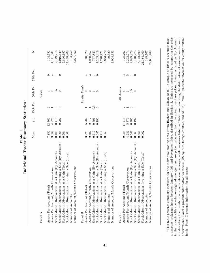
Tab

leI

Ind

ivid

ual

Tra

der

Su

mm

ary

Sta

tist

ics

a

Mea

nStd

25th

Pct

50th

Pct

75th

Pct

N

Panel

AS

tock

s

Ass

ets

Per

Acc

ount

(Tota

l)7.8

50

12.7

66

24

9104,7

52

Ass

ets

Per

Acc

ount/

Month

Obse

rvati

on

3.6

89

4.9

76

12

44,1

41,6

61

Sto

ck/M

onth

Obse

rvati

ons

at

aG

ain

(By

Acc

ount)

0.4

85

0.4

13

00.5

12,1

49,2

16

Sto

ck/M

onth

Obse

rvati

ons

Involv

ing

aSale

(By

Acc

ount)

0.0

64

0.2

07

00

04,0

16,4

49

Sto

ck/M

onth

Obse

rvati

ons

at

aG

ain

(Tota

l)0.5

04

5,8

46,1

97

Sto

ck/M

onth

Obse

rvati

ons

Involv

ing

aSale

(Tota

l)0.0

64

14,4

48,9

08

Num

ber

of

Acc

ounts

104,7

52

Num

ber

of

Acc

ount/

Month

Obse

rvati

ons

15,2

77,0

62

Panel

BE

quit

yF

un

ds

Ass

ets

Per

Acc

ount

(Tota

l)3.9

28

5.2

02

12

440,3

20

Ass

ets

Per

Acc

ount/

Month

Obse

rvati

on

2.4

02

2.3

17

12

31,2

50,4

67

Sto

ck/M

onth

Obse

rvati

ons

at

aG

ain

(By

Acc

ount)

0.7

17

0.3

91

0.5

11

757,8

53

Sto

ck/M

onth

Obse

rvati

ons

Involv

ing

aSale

(By

Acc

ount)

0.0

45

0.1

90

00

01,2

05,4

19

Sto

ck/M

onth

Obse

rvati

ons

at

aG

ain

(Tota

l)0.7

19

1,7

70,7

21

Sto

ck/M

onth

Obse

rvati

ons

Involv

ing

aSale

(Tota

l)0.0

50

2,8

43,7

72

Num

ber

of

Acc

ounts

40,3

20

Num

ber

of

Acc

ount/

Month

Obse

rvati

ons

3,0

04,1

33

Panel

CA

llA

sset

sA

sset

sP

erA

ccount

(Tota

l)9.9

84

17.4

14

25

11

128,7

07

Ass

ets

Per

Acc

ount/

Month

Obse

rvati

on

4.2

86

5.7

76

13

55,2

92,5

74

Sto

ck/M

onth

Obse

rvati

ons

at

aG

ain

(By

Acc

ount)

0.5

47

0.4

05

00.5

12,8

89,8

79

Sto

ck/M

onth

Obse

rvati

ons

Involv

ing

aSale

(By

Acc

ount)

0.0

60

0.1

97

00

05,1

40,2

75

Sto

ck/M

onth

Obse

rvati

ons

at

aG

ain

(Tota

l)0.5

56

8,7

42,4

90

Sto

ck/M

onth

Obse

rvati

ons

Involv

ing

aSale

(Tota

l)0.0

62

21,3

84,9

09

Num

ber

of

Acc

ounts

128,7

07

Num

ber

of

Acc

ount/

Month

Obse

rvati

ons

22,6

81,4

69

aT

his

table

pre

sents

sum

mary

stati

stic

sfo

rth

ein

div

idual

tradin

gdata

(fro

mB

arb

erand

Odea

n(2

000),

asa

mple

of

128,8

09

acc

ounts

from

adis

count

bro

ker

age

house

bet

wee

nJanuary

1991

and

Nov

emb

er1996),

des

crib

edin

Sec

tion

3.

Gain

sare

mea

sure

dby

com

pari

ng

the

pri

cein

that

month

wit

hth

evolu

me-

wei

ghte

dav

erage

purc

hase

pri

ce,

calc

ula

ted

from

the

act

ual

purc

hase

pri

ces.

Mea

sure

slist

edas

‘By

Acc

ount’

are

des

crib

ing

the

dis

trib

uti

on

of

acc

ount-

level

aver

ages

,w

hile

mea

sure

slist

edas

‘Tota

l’are

des

crib

ing

the

dis

trib

uti

on

of

ass

et-a

ccount-

month

obse

rvati

ons.

Panel

Apre

sents

info

rmati

on

for

stock

s(U

Seq

uit

ies,

fore

ign

equit

ies,

and

AD

Rs)

.P

anel

Bpre

sents

info

rmati

on

for

equit

ym

utu

al

funds.

Panel

Cpre

sents

info

rmati

on

for

all

ass

ets.

41

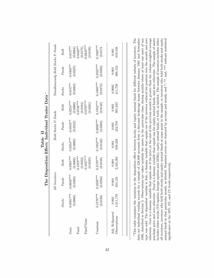
Tab

leII

Th

eD

isp

osi

tion

Eff

ect:

Ind

ivid

ual

Tra

der

Data

a

All

Inve

sto

rsH

old

Sto

cks

&F

un

ds

Sim

ult

an

eou

sly

Ho

ldS

tock

s&

Fu

nd

s

Sto

cks

Fu

nd

sB

oth

Sto

cks

Fu

nd

sB

oth

Sto

cks

Fu

nd

sB

oth

Gain

0.0

391***

-0.0

656***

0.0

391***

0.0

254***

-0.0

543**

0.0

254***

0.0

157**

-0.0

485**

0.0

157**

(0.0

066)

(0.0

260)

(0.0

066)

(0.0

060)

(0.0

222)

(0.0

060)

(0.0

064)

(0.0

225)

(0.0

064)

Fund

0.1

079***

0.0

746***

0.0

428**

(0.0

222)

(0.0

194)

(0.0

175)

Fund*G

ain

-0.1

047***

-0.0

797***

-0.0

642***

(0.0

235)

(0.0

201)

(0.0

199)

Const

ant

0.2

170***

0.3

249***

0.2

170***

0.1

952***

0.2

698***

0.1

952***

0.1

888***

0.2

316***

0.1

888***

(0.0

188)

(0.0

356)

(0.0

188)

(0.0

140)

(0.0

303)

(0.0

140)

(0.0

173)

(0.0

308)

(0.0

173

Adj.

R-S

quare

d0.0

02

0.0

04

0.0

04

0.0

01

0.0

03

0.0

02

0.0

002

0.0

03

0.0

01

Obse

rvati

ons

1,8

11,1

76

354,1

25

2,1

65,3

01

639,2

29

252,7

04

891,9

33

411,7

28

206,1

52

619,5

28

aT

his

table

exam

ines

the

vari

ati

on

inth

edis

posi

tion

effec

tb

etw

een

stock

sand

equit

ym

utu

al

funds

for

diff

eren

tsu

bse

tsof

inves

tors

.T

he

data

are

indiv

idual

tradin

gre

cord

sfo

ra

sam

ple

of

128,8

09

acc

ounts

from

adis

count

bro

ker

age

house

bet

wee

nJanuary

1991

and

Nov

emb

er1996,

des

crib

edin

Sec

tion

3.

Obse

rvati

ons

are

taken

month

lyfo

rass

ets

inth

epart

icula

rcl

ass

,duri

ng

month

sw

her

eat

least

one

ass

etof

any

typ

ew

as

sold

.T

he

dep

enden

tva

riable

isS

ale

,a

dum

my

vari

able

that

equals

one

ifth

ein

ves

tor

reduce

dhis

posi

tion

over

the

month

and

zero

oth

erw

ise.

Ga

inis

adum

my

vari

able

that

equals

one

ifth

epri

ceat

the

end

of

the

pre

vio

us

month

isgre

ate

rth

an

the

volu

me-

wei

ghte

dav

erage

purc

hase

pri

ceand

zero

oth

erw

ise.

Fu

nd

isa

dum

my

vari

able

that

equals

one

for

equit

ym

utu

al

funds,

and

zero

oth

erw

ise.

The

sam

ple

of

ass

ets

incl

udes

eith

erst

ock

s(U

Seq

uit

ies,

fore

ign

equit

ies

and

AD

Rs)

,eq

uit

ym

utu

al

funds,

or

both

,as

lab

eled

.T

he

sam

ple

of

inves

tors

incl

udes

eith

erall

inves

tors

,in

ves

tors

who

hel

db

oth

stock

sand

equit

ym

utu

al

funds

at

som

ep

oin

tin

the

sam

ple

,or

inves

tors

who

hel

db

oth

stock

sand

equit

ym

utu

al

funds

inth

at

part

icula

rm

onth

,as

lab

eled

.Sta

ndard

erro

rsare

clust

ered

by

acc

ount

and

month

,and

*,

**,

and,

***

indic

ate

stati

stic

al

signifi

cance

at

the

10%

,5%

,and

1%

level

sre

spec

tivel

y.

42

Table IIIThe Disposition Effect by Asset Type 15

Delegated? Coefficient on Gain σ Obs.

Warrants No 0.1414*** (0.0219) 5,066Foreign (Canadian) No 0.0570*** (0.0098) 55,446US Company Shares No 0.0388*** (0.0071) 1,665,017Real Estate Trust Yes 0.0348 (0.0512) 730Foreign (Ordinaries) No 0.0344* (0.0200) 15,901Units No 0.0276 (0.0429) 783ADR No 0.0235 (0.0200) 74,812Convertible Preferred No 0.0060 (0.0151) 11,703Closed-End Mutual Funds Yes 0.0026 (0.0141) 120,099Master Limited Partnership No -0.0012 (0.0103) 21,310Mutual Funds (In-House) Yes -0.0263 (0.0332) 41,046Option Equity No -0.0285* (0.0162) 21,642Options Index No -0.0312 (0.0562) 1,647Preferred Stock No -0.0351** (0.0145) 15,979Marketplace Load Equity Funds Yes -0.0366 (0.0316) 4,518Marketplace Load Bond Funds Yes -0.0486 (0.0572) 480Bond Mutual Funds Yes -0.0492* (0.0265) 16,314One Source Bond Funds Yes -0.0525** (0.0222) 34,621One Source Equity Funds Yes -0.0614** (0.0283) 246,927Ex One Source Bond Funds Yes -0.0749 (0.0474) 2,185Equity Mutual Funds Yes -0.0806*** (0.0214) 85,846Ex One Source Equity Funds Yes -0.0844*** (0.0295) 16,834

43

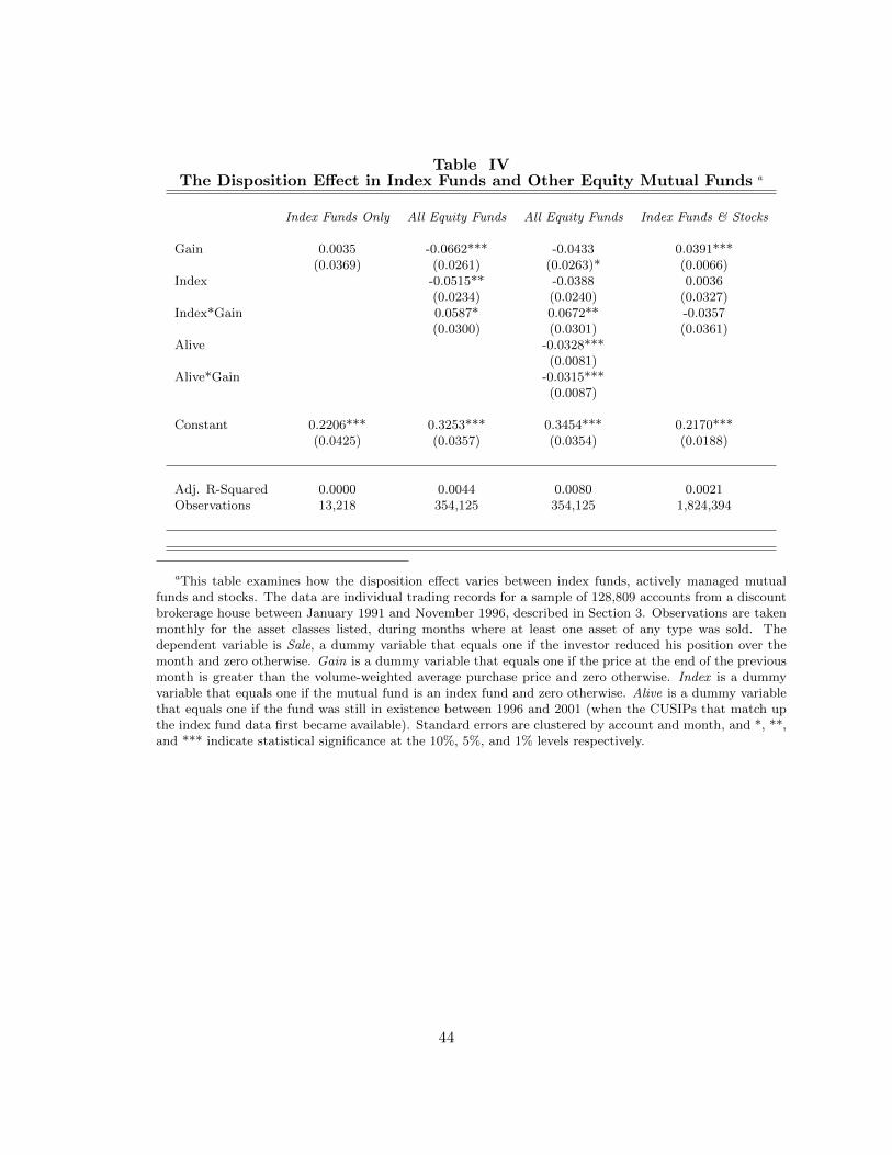
Table IVThe Disposition Effect in Index Funds and Other Equity Mutual Funds a

Index Funds Only All Equity Funds All Equity Funds Index Funds & Stocks

Gain 0.0035 -0.0662*** -0.0433 0.0391***(0.0369) (0.0261) (0.0263)* (0.0066)

Index -0.0515** -0.0388 0.0036(0.0234) (0.0240) (0.0327)

Index*Gain 0.0587* 0.0672** -0.0357(0.0300) (0.0301) (0.0361)

Alive -0.0328***(0.0081)

Alive*Gain -0.0315***(0.0087)

Constant 0.2206*** 0.3253*** 0.3454*** 0.2170***(0.0425) (0.0357) (0.0354) (0.0188)

Adj. R-Squared 0.0000 0.0044 0.0080 0.0021Observations 13,218 354,125 354,125 1,824,394

aThis table examines how the disposition effect varies between index funds, actively managed mutualfunds and stocks. The data are individual trading records for a sample of 128,809 accounts from a discountbrokerage house between January 1991 and November 1996, described in Section 3. Observations are takenmonthly for the asset classes listed, during months where at least one asset of any type was sold. Thedependent variable is Sale, a dummy variable that equals one if the investor reduced his position over themonth and zero otherwise. Gain is a dummy variable that equals one if the price at the end of the previousmonth is greater than the volume-weighted average purchase price and zero otherwise. Index is a dummyvariable that equals one if the mutual fund is an index fund and zero otherwise. Alive is a dummy variablethat equals one if the fund was still in existence between 1996 and 2001 (when the CUSIPs that match upthe index fund data first became available). Standard errors are clustered by account and month, and *, **,and *** indicate statistical significance at the 10%, 5%, and 1% levels respectively.

44

Table VTrader Characteristics by Treatment a

Panel A Funds Stocks

Male 0.55 0.60Class Level 3.37 3.48Business Major 0.66 0.67Owns Stocks 0.19 0.25Owns Funds 0.11 0.12Investing Experience 0.55 0.52

N 257 263

Panel B FundsFire Story Both None

Male 0.55 0.49 0.52 0.49Class Level 3.35 3.38 3.32 3.34Business Major 0.68 0.68 0.77 0.68Owns Stocks 0.17 0.18 0.16 0.22Owns Funds 0.09 0.10 0.07 0.11Investing Experience 0.53 0.58 0.60 0.54

N 116 125 56 72

Panel C StocksFire Story Both None

Male - 0.60 - 0.59Class Level - 3.52 - 3.43Business Major - 0.66 - 0.67Owns Stocks - 0.21 - 0.30Owns Funds - 0.11 - 0.13Investing Experience - 0.49 - 0.56

N - 141 - 122

aThis table presents summary statistics for an experiment where 514 undergraduate students tradedeither 30 mutual funds or 30 stocks at daily closing prices over a period of 12 weeks, as described in Section4. Fire and Story are the two randomized treatment conditions, described in section Section 4. ‘Class Level’is the year of the student in their degree. ‘Owns Stocks’ and ‘Owns Funds’ refer to whether the studentowns either stocks or mutual funds in real life. ‘Investing Experience’ is the student’s self-rated score oftheir investing experience. In all cases, baseline characteristics are not statistically distinguishable acrossany treatment arms. 19 students had class year variables of “other” and were not included in the Class Yearsummary statistic.

45

Table VIThe Experimental Disposition Effect For Funds a

Gain -0.141** -0.0594 -0.048 -0.000771(0.0553) (0.067) (0.061) (0.0655)

Fire 0.116 0.106(0.0987) (0.0957)

Gain*Fire -0.211** -0.174*(0.103) (0.104)

Story 0.0655 0.0396(0.0895) (0.0832)

Gain*Story -0.211** -0.173**(0.0883) (0.0877)

Constant 0.527*** 0.481*** 0.497*** 0.468***(0.0547) (0.0674) (0.0631) (0.0742)

Adj. R-squared 0.012 0.02 0.029 0.034Observations 2,011 1,957 1,957 1,957

aThis table presents the results of regressions examining how the disposition effect in mutual fundsvaries with two randomized treatments affecting delegation and cognitive dissonance. An experiment wasconducted in which 257 undergraduate students traded 30 mutual funds at daily closing prices over a periodof 12 weeks, as described in Section 4. Observations are taken daily for all funds in the student’s portfolio,on days where the student sold at least one fund. The dependent variable is Sale, a dummy variable thatequals one if the student reduced his position in the fund that day and zero otherwise. Gain is a dummyvariable that equals one if the price on the previous day is greater than the volume-weighted average purchaseprice and zero otherwise. Fire is a dummy variable for the Fire treatment. This is designed to increase thesalience of the fund manager, by replacing “Buy”, “Sell”, and “Portfolio performance/gain/loss” replacedwith the words “Hire”, “Fire”, and “Fund Manager’s performance/gain/loss” throughout the website. Storyis a dummy variable for the Story treatment. This is designed to increase the cognitive dissonance thatparticipants feel when they face a loss. All subjects must list a reason for purchasing each asset, and treatedsubjects are reminded of their previously stated reasons on the portfolio screen and the sell screen. Bothtreatments are described in more detail in Section 4. Standard errors are clustered by student and day, and*, **, and *** indicate statistical significance at the 10%, 5%, and 1% levels respectively.

46

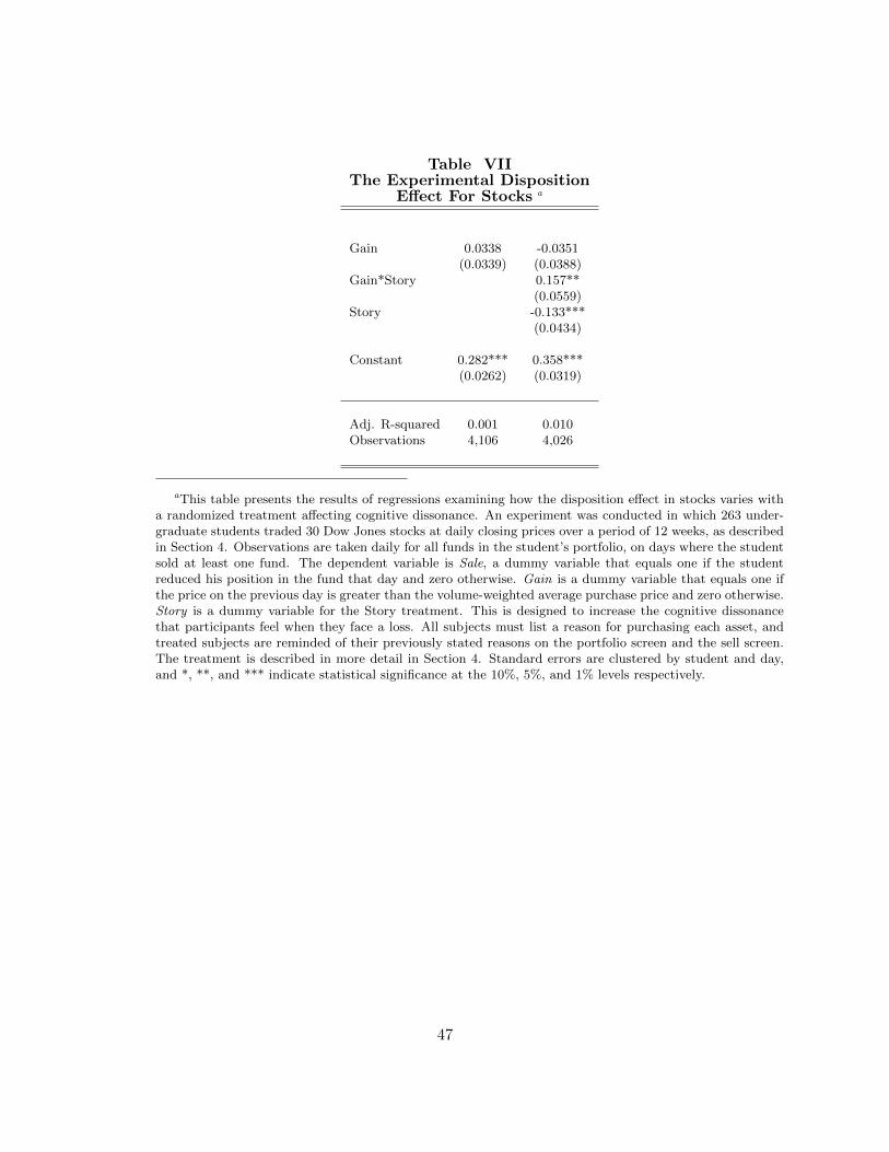
Table VIIThe Experimental Disposition

Effect For Stocks a

Gain 0.0338 -0.0351(0.0339) (0.0388)

Gain*Story 0.157**(0.0559)

Story -0.133***(0.0434)

Constant 0.282*** 0.358***(0.0262) (0.0319)

Adj. R-squared 0.001 0.010Observations 4,106 4,026

aThis table presents the results of regressions examining how the disposition effect in stocks varies witha randomized treatment affecting cognitive dissonance. An experiment was conducted in which 263 under-graduate students traded 30 Dow Jones stocks at daily closing prices over a period of 12 weeks, as describedin Section 4. Observations are taken daily for all funds in the student’s portfolio, on days where the studentsold at least one fund. The dependent variable is Sale, a dummy variable that equals one if the studentreduced his position in the fund that day and zero otherwise. Gain is a dummy variable that equals one ifthe price on the previous day is greater than the volume-weighted average purchase price and zero otherwise.Story is a dummy variable for the Story treatment. This is designed to increase the cognitive dissonancethat participants feel when they face a loss. All subjects must list a reason for purchasing each asset, andtreated subjects are reminded of their previously stated reasons on the portfolio screen and the sell screen.The treatment is described in more detail in Section 4. Standard errors are clustered by student and day,and *, **, and *** indicate statistical significance at the 10%, 5%, and 1% levels respectively.

47

Table VIIIExit Questionnaire: Funds a

Panel AOwn Skill Learning Willingness to Invest

Self Manager Any Owned

Fire -0.098 0.151 -0.181 0.330 -0.397(0.225) (0.224) (0.270) (0.289) (0.287)

Story 0.005 -0.389 -0.115 0.339 0.055(0.225) (0.224) (0.270) (0.288) (0.0287)

Constant 5.12*** 6.87*** 6.02*** 5.89*** 5.89***(0.186) (0.186) (0.223) (0.238) (0.237)

Adj. R-squared 0.008 0.006 0.006 0.002 0.000Observations 242 243 243 242 240

Panel BOwn Skill Learning Willingness to Invest

Self Manager Any Owned

Profit -0.131 -1.011 -1.338 0.048 0.518(0.405) (0.413)** (0.498)*** (0.541) (0.520)

Fire -0.167 0.186 -0.665 0.454 -1.101(0.408) (0.417) (0.503) (0.546) (0.524)**

Fire*Profit 0.159 -0.014 0.712 -0.162 1.025(0.482) (0.491) (0.593) (0.645) (0.620)*

Story -1.116 -1.503 -1.276 0.125 -0.107(0.408)*** (0.416)*** (0.502)** (0.545) (0.523)

Story*Profit 1.632 1.531 1.622 0.305 0.347(0.482)*** (0.491)*** (0.593)*** (0.645) (0.619)

Constant 5.197 7.612 6.999 5.854 5.470(0.346)*** (0.685)*** (0.426)*** (0.463)*** (0.444)***

Adj. R-squared 0.08 0.06 0.04 0.01 0.08Observations 242 243 243 242 240

aThis table examines how self-reported learning about trading mutual funds varies with the two treat-ments in the trading experiment, as described in Section 4. At the conclusion of the experiment, studentsevaluated, on a 1-10 scale, their own skill, how much they learned about their own skill and the skill of themanagers of the funds they purchased, and their willingness to invest in funds in general and the actualfunds they purchased. In Panel A, these survey responses are regressed on the treatment condition thestudent was assigned. Fire is a dummy variable for the Fire treatment. Story is a dummy variable for theStory treatment. In Panel B, the Story and Fire variables are interacted with Profit, a dummy variable thatequals one if the student finished the experiment with a total portfolio gain and zero otherwise. Standarderrors are clustered by student and day, and *, **, and *** indicate statistical significance at the 10%, 5%,and 1% levels respectively.

48

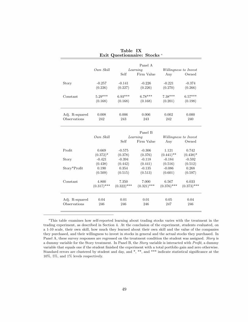
Table IXExit Questionnaire: Stocks a

Panel AOwn Skill Learning Willingness to Invest

Self Firm Value Any Owned

Story -0.257 -0.141 -0.226 -0.221 -0.374(0.226) (0.227) (0.226) (0.270) (0.266)

Constant 5.29*** 6.93*** 6.78*** 7.38*** 6.57***(0.168) (0.168) (0.168) (0.201) (0.198)

Adj. R-squared 0.008 0.006 0.006 0.002 0.000Observations 242 243 243 242 240

Panel BOwn Skill Learning Willingness to Invest

Self Firm Value Any Owned

Profit 0.669 -0.575 -0.306 1.121 0.742(0.372)* (0.378) (0.376) (0.441)** (0.438)*

Story -0.421 -0.394 -0.118 -0.184 -0.592(0.438) (0.442) (0.441) (0.516) (0.512)

Story*Profit 0.190 0.354 -0.135 -0.086 0.268(0.509) (0.515) (0.513) (0.601) (0.597)

Constant 4.800 7.350 7.000 6.567 6.033(0.317)*** (0.322)*** (0.321)*** (0.376)*** (0.373)***

Adj. R-squared 0.04 0.01 0.01 0.05 0.04Observations 246 246 246 247 246

aThis table examines how self-reported learning about trading stocks varies with the treatment in thetrading experiment, as described in Section 4. At the conclusion of the experiment, students evaluated, ona 1-10 scale, their own skill, how much they learned about their own skill and the value of the companiesthey purchased, and their willingness to invest in stocks in general and the actual stocks they purchased. InPanel A, these survey responses are regressed on the treatment condition the student was assigned. Story isa dummy variable for the Story treatment. In Panel B, the Story variable is interacted with Profit, a dummyvariable that equals one if the student finished the experiment with a total portfolio gain and zero otherwise.Standard errors are clustered by student and day, and *, **, and *** indicate statistical significance at the10%, 5%, and 1% levels respectively.

49

Appendix for

Looking for Someone to Blame:

Delegation, Cognitive Dissonance, and the

Disposition Effect

Tom ChangUniversity of Southern California

David H. SolomonUniversity of Southern California

Mark M. WesterfieldUniversity of Washington

April 2014

In this appendix, we present a three-period model that formalizes our ‘model of words’

in Section 2 (in Appendix A). We follow this with extensions and robustness checks of our

empirical work on individual trading data in Section 3 (in Appendix B). We conclude with

a list of mutual funds from the experiment and screen-shots that show visually the effects

of the treatments (in Appendix C).

A A Simple Model

Our model is based on a simplified version of the realization utility model of Barberis and

Xiong (2009, 2012) (henceforth BX) in a partial equilibrium setting, and departs from BX

in two important ways. First, in addition to receiving utility from realized losses, investors

are also assumed to experience a portion of this psychological cost, even if the asset is

not sold (i.e. from paper losses). The cost to paper losses is designed to capture the

idea that traders are able to imperfectly fool themselves regarding an unrealized loss and

thereby partially avoid the ego cost of being wrong. This difference between the investor’s

utility from realized and paper losses is the result of (un-modeled) mental tricks and defense

mechanisms that downgrade the importance of new information (the price decline) – i.e.

the difference between realized and paper losses is the result of the “second way of dealing

with cognitive dissonance,” described in Section 2, namely distorting or disregarding the

information that the asset has fallen in price in the case of paper losses. Second, we assume

that the size of the utility jolt investors receive when realizing gains and losses is a function

of not only the magnitude of the gain/loss but also the degree to which the individual feels

responsible for the original purchase decision. This results from the “third way of dealing

with cognitive dissonance” described in Section 2, namely adding an additional ameliorating

cognition.

We will work in a 3 period (t ∈ {0, 1, 2}), discrete time framework. There is a continuous

unit mass of investors, indexed by i, each of whom starts at time t = 0 with wealth W0. In

1

each time t ∈ {0, 1} the investor chooses between a riskless constant return asset and a risky

stock. The investor cannot short either asset. In the final period, the investor consumes

W2, and for simplicity we will assume all investors are risk neutral in terminal consumption.

Without loss of generality, we normalize the price of the risky asset using the risk-free

asset (alternately, we normalize the risk-free rate to zero). Then

PtPt−1

= 1 + µi,t−1 + εt−1, (6)

where µi,t−1 is investor i’s posterior expected return (described later) and εt−1 is mean-zero

noise.

At time t = {0, 1} the investor can choose to allocate his wealth between the risk-free

asset and the risky asset. The investor’s wealth therefore evolves according to

Wi,t = Wi,t−1 +Wi,t−1xi,t−1

(PtPt−1

− 1

), (7)

where xi,t−1 is the fraction of the investor’s wealth invested in the risky asset.

Finally, we will assume that at time t = 1, before trading, each investor receives a

personal shock to their valuation of the risky asset. This “value shock” has been modeled

many ways in past literature: as a posterior belief after receiving a private signal (e.g.

Grossman (1976) or Grossman and Stiglitz (1980)); as a liquidity shock or as an outside

income shock (e.g. Pagano (1989)); as a noise trader belief shock (e.g. De Long et al.

(1990)). What is important for this model is that investors have heterogenous valuations

and so there is a reason for trade. Regardless of the source, this shock changes the posterior

expected return for each investor, with

µi,1 ∼ cdf G(µ) (8)

2

where G(µ) is the cumulative density function that describes the posterior distribution.

We assume, as suggested by the law of large numbers with a continuous unit mass of

investors, that the posteriors µi,1 are distributed exactly as described by G. For example,

if µi,t ∼ U [−1, 1], then G(µ) = 12µ + 1

2 and there is exactly a measure of 12 investors at

each µi,1 ∈ [−1, 1]. For simplicity, we assume that µi,0 = E [µi,1], the same constant for

all investors. We extend the value shock to allow correlation with prices (e.g. learning,

momentum, price-targeting) in Section A.3.

A.1 The Costs of Being Wrong

Into this simple model, we introduce a psychological cost based on cognitive dissonance

theory and modeled on BX. The investor is at a loss at t = 1 if he bought the risky asset

and it declined in price: Li,t ≡ min{0, Pt−Pt−1} ≤ 0.1 The psychological cost is a disutility

from being wrong, and its base value is φLi,t, where φ ≥ 0 is a measure of the ‘ego’ cost

the investor experiences from having to admit that he made a mistake. It is the dissonance

between having bought the stock and having that stock now at a loss that the investor will

seek to alleviate.

First, the investor can update his beliefs about his own skill as an investor to reflect the

new information, as in the “first way of dealing with cognitive dissonance” from Section 2,

by changing one of the cognitions to make them consistent with each other. By assumption,

this does not happen. Instead, the investor will use one of the other two methods.

The investor can try to alleviate dissonance by convincing oneself that the new infor-

mation in the price decline is unimportant or irrelevant, as per the “second way” of dealing

with cognitive dissonance from Section 2. Thus the investor can choose to hold the existing

asset (or buy more), and try to ‘fool himself’ that the loss is not real. The investor then

1Our results are robust to measuring the loss in other ways, e.g. as dollars lost (Li,t =

xi,t−1Wi,t−1

Pt−1min{0, Pt − Pt−1}), or fraction of wealth lost(Li,t = xi,t−1

1Pt−1

min{0, Pt − Pt−1}).

3

realizes disutility

λφLi,t. (9)

where λ ∈ [0, 1] measures the extent to which an investor must pay the ‘ego cost’ of being

wrong if he does not realize his losses. This means the investors experience a psychological

cost from paper losses due to the realization that they have made a mistake. That is, even

if the individual does not realize the loss, the fact of the loss itself causes the trader to

experience a fraction of the negative utility he would receive in realizing the loss.

As an alternative, the investor can choose to realize the loss and sell the asset. However,

this implies the investor pays the full ego cost of being wrong unless he or she brings in

a third cognition: the loss is someone else’s fault. If the investor is able to bring such an

ameliorating cognition to bear (i.e. find a scapegoat), then the individual can sell the asset

without experiencing the realization utility associated with admitting he was wrong. Thus

the realization utility from selling an asset at a loss can be reduced from φLi,t to

(1− θ)φLi,t (10)

where θ ∈ [0, 1] parameterizes the extent to which loss-disutility can be lessened by blaming

others (i.e. the “third way” of dealing with cognitive dissonance from Section 2. θ formalizes

the salience of a scapegoat.

A.2 The Optimal Trading Strategy

We will solve for optimal holdings by backwards induction. At time t = 1, each investor

receives his signal and must decide whether to change his allocation to the risky asset. At

4

time t = 0, each investor faces an unconditional optimization. The investor solves

J(t = 1,Wi,1, xi,0) = maxxi,1

[(λ1hold,buy + (1− θ)1sell)φLi,1 + Ei[Wi,2]] (11)

J(t = 0,Wi,0) = maxxi,0

E0 [J(1,Wi,1, xi,0)] (12)

At t = 0, all investors are the same, and so xi,0 = x0, Li,1 = L1, and Wi,1 = W1. Because of

the kink in the utility function at {t = 1, L = 0}, the investor is risk averse at t = 0 despite

being risk-neutral over period-2 consumption. We will further assume that asset returns

and G are such that 0 < x0 < 1, although this is not critical for the results.

If an agent has experienced a gain (L1 = 0), then he simply wants to maximize his

terminal wealth. He will invest all of his wealth in the risky asset if µi,1 > 0 and all his

wealth in the riskless asset otherwise. Thus the probability that the agent sells conditional

on a gain is G(µ = 0).

If the agent is at a loss, then he acts to maximize the change in his wealth over the next

period and his psychological utility today:

maxxi,1

(λ1hold,buy + (1− θ)1sell)φL1 +W1xi,1µi,1 (13)

The agent will choose to invest all of his wealth in the risky asset if

φλL1 + µi,1W1 > φ(1− θ)L1 (14)

and will sell all of his holdings in the risky asset otherwise. Thus, the probability that the

agent sells conditional on a loss is G(µ = φ (1− θ − λ) L1

W1

).

The magnitude of the disposition effect is the difference between the probability of selling

5

conditional on a gain minus the probability of selling conditional on a loss:

DE ≡ G(0)−G(φ (1− θ − λ)

L1

W1

). (15)

where we say there is a reverse disposition effect if DE < 0. Because G is a cdf and L1 ≤ 0,

we have

∂

∂θDE =

∂

∂λDE = G′

(φ (1− θ − λ)

L1

W1

)φL1

W1< 0 (16)

∂

∂φDE = −G′

(φ (1− θ − λ)

L1

W1

)(1− θ − λ)

L1

W1(17)

where the sign follows from L1 < 0. ∂∂φDE is positive when θ is small (i.e. there is not

a salient person to blame when realizing losses, such as for stocks) and negative when θ is

large (i.e. when there is a salient scapegoat, such as a fund manager).

A.3 Learning from Prices

We now extend the simple model to allow the distribution of value shocks (G(µ)) to depend

on past returns. This extension allows us to capture learning, asset-price momentum, a

belief in mean-revision, price targeting, and other, similar, mechanisms. We write

µi,1 ∼ cdf G

(µ;P1

P0

). (18)

For learning and momentum, in which higher past returns raise the value of µi,1, we

have ∂∂P1

G < 0. For mean-reversion and price targeting, for which higher past returns lower

the value of µi,1, we have ∂∂P1

G > 0. The expected magnitude of the disposition effect is

then

EDE ≡ E[G(0;P1)|L1 = 0

]− E

[G

(φ (1− θ − λ)

L1

W1;P1

)∣∣∣∣L1 < 0

]. (19)

6

The comparative statics on EDE for θ and λ have the same sign as for DE (16). For φ,

we have

∂

∂φEDE = −E

[G′(φ (1− θ − λ)

L1

W1;P1

)(1− θ − λ)

L1

W1

∣∣∣∣L1 < 0

]. (20)

Aside from confirming the direction of the comparative statics, adding a relationship

between the functional form of G and P1 implies that the expected disposition effect is no

longer near zero for nearly rational agents (φ ≈ 0). If G is decreasing in P1 (e.g. learning or

momentum), then (P1|L1 = 0) > (P1|L1 < 0) implies that the expected disposition effect

is negative for nearly rational agents (i.e. agents who experience very little psychological

discomfort from losses: φ ≈ 0). In contrast, if G is increasing in P1 (e.g. mean reversion or

price targeting), then the expected disposition effect is positive for nearly rational agents.

In either case, however, inspection of (19) shows that the expected disposition effect is

positive when φ is large and θ is small (i.e. admitting mistakes is costly and there is not a

salient scapegoat), and negative when φ is large and θ is large (i.e. admitting mistakes is

costly and there is a salient scapegoat to blame for the realized losses), as in the baseline

case.

A.4 Model Predictions

A key result of the model is that the extent to which a trader can blame his poor performance

on someone else will be associated with the disposition effect. We assume that for assets

like stocks, it is difficult to scapegoat others for one’s mistakes when trading individual

stocks (low θ). In contrast, with actively managed funds, the fund manager is an easy

scapegoat for poor fund asset performance (high θ). Thus, we predict that for φ ≥ 0 an

investor will display a positive disposition effect in trading non-delegated assets (like stocks)

and a reverse-disposition effect in trading delegated assets like funds. In addition, trader

behavior approaches the neoclassical case as φ approaches zero as losses do not impose extra

7

psychological costs. Thus we predict that an investor, regardless of the type of asset, will

exhibit no disposition effect in cases where “ego” is not at stake.

The experimental treatments involve changing the psychological costs of admitting being

wrong (φ) and the degree to which traders blame fund managers for poor performance (θ).

The first treatment ‘Story’ is designed to increase the overall level of cognitive dissonance

(φ). As such, this one treatment should increase the magnitude of the deposition effect

for non-delegated assets while increasing the magnitude of the reverse-disposition effect

for delegated assets.2 The second treatment ‘Fire’ is designed to make the manager more

salient, and thus more easily (or often) blamed for bad results (i.e. higher θ). Such an

increase in θ should lead to a larger reverse-disposition effect when trading funds.3

Hence we predict that:

1. Assets that are delegated portfolios will display a reverse-disposition effect, while those

that are not delegated will display a disposition effect. This difference is due to the

psychological effects of delegation rather than the economic effects.

2. If investors have a higher level of cognitive dissonance, they will display a larger

disposition effect in non-delegated assets like stocks and a larger reverse-disposition

effect in delegated assets like funds. Similarly investors with low levels of cognitive

dissonance will display little to no disposition effect.

3. If investors focus more on the role of the fund manager instead of their own role, they

2While we assume that the Story treatment affects only φ, this assumption is not necessary. From (15),the magnitude of the disposition effect is increasing in φ(1 − θ − λ). Thus for θ ≈ 0, a treatment thatincreases φ and λ will increase the disposition effect if ∆φ(1 − λ) − (φ + ∆φ)∆λ > 0, which is met aslong as ∆λ is less than some threshold ∆λ > 0. Similarly for θ ≈ 1, an increase in φ will decrease themagnitude of the disposition effect (increase the magnitude of the reverse disposition effect) if ∆λ is greaterthan some threshold ∆λ < 0. A treatment that increases φ will have the opposite effect on the dispositioneffect for delegated vs. non-delegate assets as long as it doesn’t simultaneously change λ “too much” (i.e.∆λ < ∆λ < ∆λ.

3One potential concern with this treatment is that is affects φ along with θ. While we do not believethis to be the case, we also note that since the change in the disposition effect in that case is given by∆φ(1− θ − λ)− (φ+ ∆φ)∆θ, the treatment must induce a large decrease in φ to reverse the prediction.

8

will display a larger reverse-disposition effect.

B Extensions and Robustness Checks for Empirical Results

B.1 Volatility, Horizon, and Position Size Effects

While our focus has been on delegation, one might be concerned that there are other

differences between mutual funds and stocks that drive the levels of the disposition effect.

The first possibility is the effect of return volatility. Both Ben-David and Hirshleifer

(2012) and Kaustia (2010b) report that the propensity to sell is not flat across the domain of

gains and losses, while Linnainmaa (2010) points out that sell limit orders can mechanically

generate “a trading pattern that is observationally equivalent to the disposition effect.” In

such a case, assets with high volatility are likely to have returns which place them in regions

with different propensities to sell, and this may drive the measured disposition effect even if

the overall relationship between returns and selling propensity is the same for both assets.

Second, there may be differences in the investing horizon between investors in delegated

and non-delegated assets. Within equities, Ben-David and Hirshleifer (2012) report that

the length of the holding period affects the level of the disposition effect, and it may be

that differences in the holding periods for delegated and non-delegated assets are driving

the apparent difference in the disposition effect.

Finally, there may be differences in the overall portfolio importance of delegated and

non-delegated assets. Investors may hold a larger or smaller amount of their money in

different asset classes, and this may drive their level of attention to the asset or level of risk

displayed (particularly if the investor uses mental accounting to treat each asset separately).

In Table X, we test whether the effect of delegation survives after controlling for asset

volatility, holding period, and position size. The regressions are similar to those in Table

II but include observations of all assets from Table III (i.e. all assets other than money

9

market funds), rather than just stocks and equity mutual funds. The regressions are:

Saleijt = α+ βGainijt + γGainijt ×Delegatedj + δDelegatedj (21)

+ ζGainijt × Controlsijt + ηControlsijt + εijt,

where i is an account, j is an asset, and t is the time period. Observations are included

for all assets on days where the investor sold a position in some asset. Delegated is a

dummy variable that equals one if the asset class involves delegated portfolio management,

according to the classifications in Table III.

The vector Controls includes Volatility, Holding Period (Account), Holding Period, Log

Dollar Value (Position), and Portfolio Weight (Position). Volatility is the average volatility

of returns for that asset class, computed by taking the standard deviation of returns for each

individual security, then averaging for all securities in the particular asset class. Holding

Period (Account) is the average holding period for that account, computed as the total

length of time between the first observation for the security and the last observation for the

security, averaged across all securities in the account. Holding Period is the same holding

period but taking the average for all securities in the asset class. Log Dollar Value (Position)

is the dollar value of the position in that asset at the start of the month, while Portfolio

Weight (Position) is the weight in that security in the investor’s portfolio at the start of the

month. Interactions with the Gain variable capture whether these variables are associated

with different levels of the disposition effect.

The results are reported in Table X. They indicate that delegated assets have a sig-

nificantly lower disposition effect than other assets, over and above the effects of volatility,

holding period, and position size. The base effect of the Gain variable in column 2 is 0.0341,

with the interaction of Gain×Delegated having a coefficient of -0.0802, meaning that the

overall Gain coefficient for delegated assets is 0.0341− 0.0802 = −0.0461.

10

The interpretation of the coefficients is that non-delegated assets are 3.41% more likely to

be sold if they are at a gain, compared with a base probability of 22.1%. For non-delegated

assets, they are 4.61% less likely to be sold if they are at a gain, compared with a base

probability of being sold of 21.5%. This difference between delegated and non-delegated

assets remains significant after controlling for the asset-level volatility (column 3), asset-

level average holding period (column 4), and account-level average holding-period (column

5), log dollar value of the position (column 6), portfolio weight (column 7), as well as all of

these variables in combination (column 8).

B.2 Effects of Non-Trading Days and Weighting By Account Size

In our main specifications, the disposition effect is calculated using observations from

months when there was some sale in the account, as in Odean (1998)) and others. The

advantage of this specification is that it ensures the investor was actually paying attention

to the portfolio that month (and, moreover, desiring to make some sale). This choice of

specification has two potential disadvantages, however. First, it ignores the times when the

investor was paying attention to their portfolio, but actively chose not to sell. Such periods

are relevant when considering the overall propensity to sell winners and losers. Second, this

specification will include more observations from accounts that hold more positions. This

effect is twofold - not only will a large account have contribute more observations in each

month that a sale occurs (because every asset in a sale month is included), but a larger

account will also generate more sale months, thus magnifying the effect. This holds true

even if the overall portfolio has the same annual turnover for each stock.

We wish to make sure that neither of these aspects is driving our main trading results. To

do this, we estimate the main results from Table II, but using two alternative specifications.

The first includes all months that the investor held the asset in question (stocks or funds),

rather than just months with some sale. This will ensure that the inclusion of non-sale

11

months does not alter the assessment about the willingness of investors to sell gains versus

losses, and ensures that small account are sampled every month (i.e. at the same frequency

as large accounts).

The second specification uses a weighted least squares regression, where each observation

is weighted according to the inverse of the number of positions the investor held that month.

This is designed to reduce the larger sampling of observations from large accounts - each

account/month is thus given an equal total weight in the regression, regardless of the number

of positions the account held. This is done both for the sample that includes only months

when a sale occurs and for the sample that includes all months. This specification ensures

that the base difference between stocks and funds is not driven by drawing more observations

from accounts that have more positions.

The results are presented in Table XI. The regression specification is the same as in

Table II - regressing Sale on Gain, Fund and Gain×Fund. This is done as before variously

for i) for all accounts that held either stock or fund, ii) accounts that held both stock and

fund at some point, and iii) accounts that held both stock and fund in that month.

Columns 1-3 show the effect of weighting according to the inverse of number of positions

that month, with the sample being all months with some sale. As before, funds show a

significantly lower disposition effect relative to stocks, and this persists as the sample is

cut to include only simultaneous holders of both assets. In addition, the point estimates

for both Gain and Gain×Fund are larger in magnitude than in Table II, suggesting that

smaller accounts exhibit a larger disposition effect in stocks and a larger reverse disposition

effect in funds.

Columns 4-9 show the sample that includes all months, regardless of whether there

was a sale or not. Columns 4-6 weight each observation equally, and columns 7-9 weight

each observation by the inverse of the number of positions in the account that month.

All specifications show a significant positive coefficient on Gain and a significant negative

12

coefficient on Gain×Fund, indicating that the difference in disposition effect between stocks

and funds is not driven by the exclusion of non-trade months. The point estimates in

both coefficients are lower in columns 4-9 by construction, as the extra months added all

have values of zero for the dependent variable. In columns 7-9, weighting by the inverse

of the number of positions in the account that month again increases the coefficients on

the variables of interest, suggesting that the disposition effect in stocks and the reverse

disposition effect in funds are both larger in magnitude for traders that hold fewer assets.

B.3 Stock and Fund Difference Using Fixed Effects

The key point from Table II is that the difference in disposition effect between stocks and

funds is not driven by the sample of investors that invest in only one asset class or the other.

Another more flexible way to show the same point is to include additional account fixed

effects to control for account-level variation in trading. We do this in Table XII, including

fixed effects in different combinations. The full specification is:

Saleijt = α+ βGainijt + γGainijt × Fundj + δFundj + ζAccounti (22)

+ θGainijt ×Accounti + λFundijt ×Accounti + µDatet + εijt,

In this specification, the Account fixed effects allow for differences across accounts in the

overall selling propensity across assets, the Gain×Account interaction allows for a different

level of the disposition effect across accounts, and the Fund×Account interaction allows for

a different level of the propensity to sell funds relative to stocks across accounts. The Date

fixed effects allow for the overall selling propensity to vary in the aggregate in different

months. The regression then estimates a joint difference in the disposition effect between

stocks and funds for all accounts (Gain×Fund), after controlling for the other listed sources

variation.

13

These results are presented in Table XII. The regressions show the successive addition

of the various fixed effects does not eliminate the significance of the Gain×Fund interaction.

The Gain×Fund interaction is highly significant in all specifications, with the coefficients

(ranging from -0.0723 to -0.109) being comparable in size to those of Table II. This demon-

strates that investors show a significant difference in the disposition effect between stocks

and funds, even after controlling for numerous account-level differences in trading behavior.

B.4 Heterogeneous Effects: Experience and Gender

Though not directly related to the main goal of understanding the disposition effect through

the lens of cognitive dissonance theory, our data allows us to test the general idea that

experience can reduce the magnitude of behavioral biases.4 In this context, we examined

whether students who have more experience display lower or higher levels of the disposition

effect in stocks and the reverse-disposition effect in funds.

We use three proxies for experience: self-reported skill, enrollment in an upper level

investments class, and ownership of stocks or funds in real life. In regressions not shown, we

test whether experience reduces the level of bias by running our basic regression (Equation

1) with a each measure of experience and an interaction term between Gain and that

measure. For mutual fund traders, we find evidence that more experienced traders exhibit

a lower level of the reverse-disposition effect, with the effects being statistically significant for

self-reported experience and ownership experience, and marginally significant for students

in the Investments class. For stocks, the results are inconsistent across the measures of

experience, with students who own stocks displaying a significantly lower disposition effect,

but Investments students displaying a weakly greater disposition effect. This last result

4For example, List (2003) and List (2011) find that experienced sports card traders exhibit far less ofan endowment effect than inexperienced traders, while Haigh and List (2005) find that experienced futuresand options traders exhibit greater myopic loss aversion than student subjects. More directly related toour results, Shapira and Venezia (2001) find that brokerage professionals exhibit a smaller disposition effectthan individual traders when trading stocks.

14

does not seem to admit a clear interpretation.5

Similar to experience, a literature on gender-based differences in preferences suggests

that we might observe differences in the reaction to the treatments from men and women.6

In regressions not shown, we repeated our standard regression (Equation 1) with a dummy

for female and an interaction term between Gain and the female dummy. Consistent with

Ben-David and Hirshleifer (2012), we do not find statistically significant differences between

men and women in terms of their level of the disposition effect,7 but we do not have enough

power to rule out substantial differences between genders.

5Actual ownership of stocks and funds may be a better measure of experience than self-reported measuresor having taken more classes. This last measure may be problematic if the composition of students in theInvestments class is systematically different in ways beyond trading experience.

6See Croson and Gneezy (2009) for a recent review of the literature.

7Women display a larger disposition effect in stocks and a larger reverse-disposition effect in funds, butneither difference is significant at conventional levels. Similarly, women display a smaller response to all ofthe treatments, but the differential is not statistically significant at conventional levels.

15

C Mutual Funds & Screenshots

The funds included in the experiment were the following:

# Fund Name Ticker

1. Fidelity Contrafund FCNTX2. Fidelity Advisor New Insights I FINSX3. ING Value Choice Fund PAVAX4. Franklin Growth Adv. FCGAX5. Franklin Rising Dividends Fund FRDAX6. Janus Aspen Perkins Mid Cap Value JAMVX7. Janus Triton Fund Class A JGMAX8. American Century Equity Income A TWEAX9. American Century Mid Cap Value Inv ACMVX10. American Century Small Cap Value Inv ASVIX11. Vanguard Dividend Appreciation VDAIX12. Vanguard Dividend Growth VDIGX13. Vanguard PRIMECAP Admiral Shares VPMAX14. Dreyfus Research Growth Z DREQX15. Dreyfus Tax-Managed Growth I DPTRX16. Invesco Van Kampen SmallCapValue Y VSMIX17. Invesco Charter R CHRRX18. Invesco Diversified Dividend Investor LCEIX19. Invesco Mid Cap Core Equity I GTAVX20. JPMorgan Investor Growth Select ONIFX21. JPMorgan Small Cap Equity A VSEAX22. JPMorgan US Equity Select JUESX23. Prudential Jennison Equity Income A SPQAX24. Prudential Jennison Mid Cap Growth R JDERX25. Schroder US Opportunities Inv SCUIX26. Schroder US Small & Mid Cap Opportunities SMDIX27. ING Mid Cap Opportunities Fund NMCIX28. Wells Fargo Advantage Growth C WGFCX29. Wells Fargo Advantage Omega Growth R EKORX30. Wells Fargo Advantage Premier Large Companies EKJYX

16

Figure 1: Main portfolio screen, no treatments.

Figure 2: Main portfolio screen, Fire treatment.

17

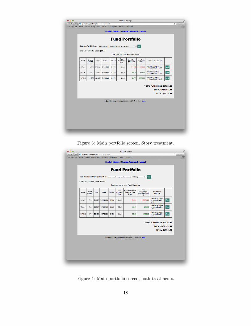
Figure 3: Main portfolio screen, Story treatment.

Figure 4: Main portfolio screen, both treatments.

18

Figure 5: Sell screen, no treatments.

Figure 6: Sell screen, Fire treatment.

19

Figure 7: Sell screen, Story treatment.

Figure 8: Sell screen, both treatments.

20

Appendix References

Barberis, N. and W. Xiong (2009). What drives the disposition effect? An analysis of along-standing preference-based explanation. Journal of Finance 64, 751–784.

Barberis, N. and W. Xiong (2012). Realization utility. Journal of Financial Economics 104,251–271.

Ben-David, I. and D. Hirshleifer (2012). Are investors really reluctant to realize theirlosses? Trading responses to past returns and the disposition effect. Review of FinancialStudies 25 (8), 2485–2532.

Croson, R. and U. Gneezy (2009). Gender differences in preferences. Journal of EconomicLiterature 47 (2), 1–27.

De Long, J. B., A. Shleifer, L. H. Summers, and R. J. Waldman (1990). Noise trader riskin financial markets. Journal of Political Economy 98 (4), 703–738.

Grossman, S. (1976). On the efficiency of competitive stock markets where traders havediverse information. Journal of Finance 31, 573–585.

Grossman, S. and J. Stiglitz (1980). On the impossibility of informationally efficient markets.American Economic Review 70 (3), 393–408.

Haigh, M. S. and J. A. List (2005). Do professional traders exhibit myopic loss aversion?An experimental analysis. Journal of Finance 60 (1), 523–534.

Kaustia, M. (2010). Prospect theory and the disposition effect. Journal of Financial andQuantitative Analysis 45 (3), 791–812.

Linnainmaa, J. (2010). Do limit orders alter inferences about investor performance andbehavior? Journal of Finance 64 (4), 1473–1506.

List, J. A. (2003). Does market experience eliminate market anomalies? Quarterly Journalof Economics 118 (1), 41–71.

List, J. A. (2011). Does market experience eliminate market anomalies? The case of exoge-nous market experience. American Economic Review (Papers and Proceedings) 101 (3),313–317.

Odean, T. (1998). Are investors reluctant to realize their losses? Journal of Finance 53 (5),1775–1798.

Pagano, M. (1989). Endogenous market thinness and stock price volatility. Review ofEconomic Studies 56 (2), 269–288.

Shapira, Z. and I. Venezia (2001). Patterns of behavior of professionally managed andindependent investors. Journal of Banking and Finance 25, 1573–1587.

21

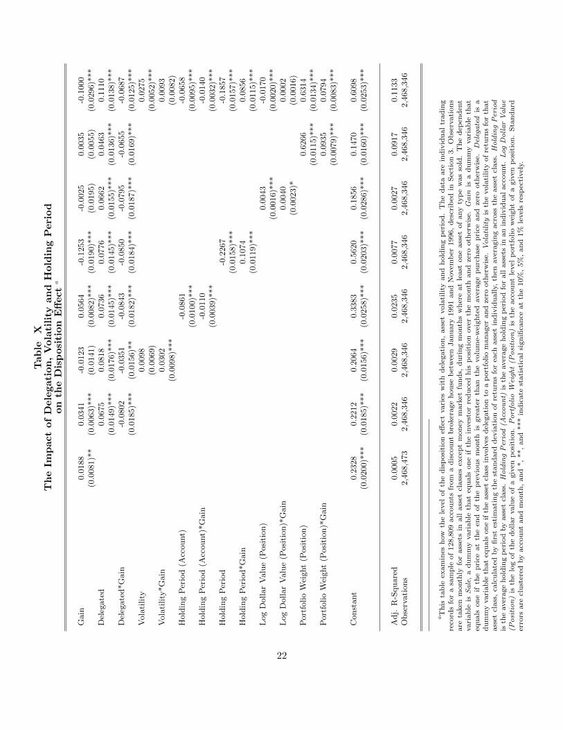
Tab

leX

Th

eIm

pact

of

Dele

gati

on

,V

ola

tility

an

dH

old

ing

Peri

od

on

the

Dis

posi

tion

Eff

ect

a

Gain

0.0

188

0.0

341

-0.0

123

0.0

564

-0.1

253

-0.0

025

0.0

035

-0.1

000

(0.0

081)*

*(0

.0063)*

**

(0.0

141)

(0.0

082)*

**

(0.0

190)*

**

(0.0

195)

(0.0

055)

(0.0

296)*

**

Del

egate

d0.0

675

0.0

818

0.0

736

0.0

776

0.0

662

0.0

463

0.1

110

(0.0

149)*

**

(0.0

176)*

**

(0.0

145)*

**

(0.0

145)*

**

(0.0

155)*

**

(0.0

136)*

**

(0.0

138)*

**

Del

egate

d*G

ain

-0.0

802

-0.0

351

-0.0

843

-0.0

850

-0.0

795

-0.0

655

-0.0

687

(0.0

185)*

**

(0.0

156)*

*(0

.0182)*

**

(0.0

184)*

**

(0.0

187)*

**

(0.0

169)*

**

(0.0

125)*

**

Vola

tility

0.0

098

0.0

275

(0.0

069)

(0.0

052)*

**

Vola

tility

*G

ain

0.0

302

0.0

093

(0.0

098)*

**

(0.0

082)

Hold

ing

Per

iod

(Acc

ount)

-0.0

861

-0.0

658

(0.0

100)*

**

(0.0

095)*

**

Hold

ing

Per

iod

(Acc

ount)

*G

ain

-0.0

110

-0.0

140

(0.0

039)*

**

(0.0

032)*

**

Hold

ing

Per

iod

-0.2

267

-0.1

857

(0.0

158)*

**

(0.0

157)*

**

Hold

ing

Per

iod*G

ain

0.1

074

0.0

856

(0.0

119)*

**

(0.0

115)*

**

Log

Dollar

Valu

e(P

osi

tion)

0.0

043

-0.0

170

(0.0

016)*

**

(0.0

020)*

**

Log

Dollar

Valu

e(P

osi

tion)*

Gain

0.0

040

0.0

002

(0.0

023)*

(0.0

016)

Port

folio

Wei

ght

(Posi

tion)

0.6

266

0.6

314

(0.0

115)*

**

(0.0

134)*

**

Port

folio

Wei

ght

(Posi

tion)*

Gain

0.0

935

0.0

794

(0.0

079)*

**

(0.0

083)*

**

Const

ant

0.2

328

0.2

212

0.2

064

0.3

383

0.5

620

0.1

856

0.1

470

0.6

098

(0.0

200)*

**

(0.0

185)*

**

(0.0

156)*

**

(0.0

258)*

**

(0.0

203)*

**

(0.0

286)*

**

(0.0

160)*

**

(0.0

253)*

**

Adj.

R-S

quare

d0.0

005

0.0

022

0.0

029

0.0

235

0.0

077

0.0

027

0.0

917

0.1

133

Obse

rvati

ons

2,4

68,4

73

2,4

68,3

46

2,4

68,3

46

2,4

68,3

46

2,4

68,3

46

2,4

68,3

46

2,4

68,3

46

2,4

68,3

46

aT

his

tab

leex

am

ines

how

the

level

of

the

dis

posi

tion

effec

tvari

esw

ith

del

egati

on

,ass

etvola

tility

an

dh

old

ing

per

iod

.T

he

data

are

ind

ivid

ual

trad

ing

reco

rds

for

asa

mp

leof

128,8

09

acc

ou

nts

from

ad

isco

unt

bro

ker

age

hou

seb

etw

een

Janu

ary

1991

an

dN

ovem

ber

1996,

des

crib

edin

Sec

tion

3.

Ob

serv

ati

on

sare

taken

month

lyfo

rass

ets

inall

ass

etcl

ass

esex

cep

tm

on

eym

ark

etfu

nd

s,d

uri

ng

month

sw

her

eat

least

on

eass

etof

any

typ

ew

as

sold

.T

he

dep

end

ent

vari

ab

leis

Sale

,a

du

mm

yvari

ab

leth

at

equ

als

on

eif

the

inves

tor

red

uce

dh

isp

osi

tion

over

the

month

an

dze

rooth

erw

ise.

Gain

isa

du

mm

yvari

ab

leth

at

equ

als

on

eif

the

pri

ceat

the

end

of

the

pre

vio

us

month

isgre

ate

rth

an

the

volu

me-

wei

ghte

daver

age

pu

rch

ase

pri

cean

dze

rooth

erw

ise.

Delegated

isa

du

mm

yvari

ab

leth

at

equ

als

on

eif

the

ass

etcl

ass

involv

esd

eleg

ati

on

toa

port

folio

man

ager

an

dze

rooth

erw

ise.

Volatility

isth

evola

tility

of

retu

rns

for

that

ass

etcl

ass

,ca

lcu

late

dby

firs

tes

tim

ati

ng

the

stan

dard

dev

iati

on

of

retu

rns

for

each

ass

etin

div

idu

all

y,th

enaver

agin

gacr

oss

the

ass

etcl

ass

.HoldingPeriod

isth

eaver

age

hold

ing

per

iod

by

ass

etcl

ass

.HoldingPeriod(A

ccount)

isth

eaver

age

hold

ing

per

iod

for

all

ass

ets

inan

ind

ivid

ual

acc

ou

nt.

Log

DollarValue

(Position)

isth

elo

gof

the

dollar

valu

eof

agiv

enp

osi

tion

.PortfolioW

eigh

t(P

osition)

isth

eacc

ou

nt

level

port

folio

wei

ght

of

agiv

enp

osi

tion

.S

tan

dard

erro

rsare

clu

ster

edby

acc

ou

nt

an

dm

onth

,an

d*,

**,

an

d***

ind

icate

stati

stic

al

sign

ifica

nce

at

the

10%

,5%

,an

d1%

level

sre

spec

tivel

y.

22

Tab

leX

IT

he

Dis

posi

tion

Eff

ect:

Ind

ivid

ual

Tra

der

Data

Rob

ust

ness

Ch

eck

sa

Mo

nth

sw

ith

So

me

Sa

leA

llM

on

ths

Wei

ghti

ng

1/

(#P

osi

tio

ns

inA

cco

un

tT

ha

tM

on

th)

Equ

al

1/

(#P

osi

tio

ns

inA

cco

un

tT

ha

tM

on

th)

All

Sto

ck&

Fu

nd

sS

tock

&F

un

ds

All

Sto

ck&

Fu

nd

sS

tock

&F

un

ds

All

Sto

ck&

Fu

nd

sS

tock

&F

un

ds

Sim

ult

an

eou

sly

Sim

ult

an

eou

sly

Sim

ult

an

eou

sly

Gain

0.0

641

***

0.0

466

***

0.0

322

***

0.0

158***

0.0

138***

0.0

103***

0.0

181***

0.0

175***

0.0

129***

0.0

095

0.0

082

0.0

080

(0.0

024)

(0.0

024)

(0.0

027)

(0.0

022)

(0.0

023)

(0.0

025)

Fund

0.1

159

***

0.0

865

***

0.0

356

*-0

.0011

-0.0

061

-0.0

083

-0.0

030

-0.0

038

-0.0

055

0.0

266

0.0

221

0.0

200

(0.0

059)

(0.0

053)

(0.0

051)

(0.0

059)

(0.0

049)

(0.0

050)

Fund*G

ain

-0.1

409

***

-0.1

091

***

-0.0

883

***

-0.0

289***

-0.0

254***

-0.0

225***

-0.0

289***

-0.0

262***

-0.0

239***

0.0

313

0.0

247

0.0

245

(0.0

068)

(0.0

062)

(0.0

065)

(0.0

068)

(0.0

059)

(0.0

064)

Const

ant

0.3

573

***

0.2

916

***

0.2

585

***

0.0

662***

0.0

687***

0.0

687***

0.0

602***

0.0

607***

0.0

611***

0.0

277

0.0

182

0.0

240

(0.0

073)

(0.0

061)

(0.0

077)

(0.0

073)

(0.0

055)

(0.0

077)

Adj.

R-S

quare

d0.0

05

0.0

03

0.0

03

0.0

01

0.0

02

0.0

02

0.0

02

0.0

02

0.0

02

Obse

rvati

ons

2,1

65,3

01

891,9

33

619,5

28

7,5

60,8

46

2,8

33,2

93

1,8

88,7

03

7,5

60,8

46

2,8

33,2

93

1,8

88,7

03

aT

his

table

exam

ines

the

vari

ati

on

inth

edis

posi

tion

effec

tb

etw

een

stock

sand

equit

ym

utu

al

funds.

The

data

are

indiv

idual

tradin

gre

cord

sfo

ra

sam

ple

of128,8

09

acc

ounts

from

adis

count

bro

ker

age

house

bet

wee

nJanuary

1991

and

Nov

emb

er1996,des

crib

edin

Sec

tion

3.

Obse

rvati

ons

are

taken

month

lyfo

rass

ets

inth

epart

icula

rcl

ass

,duri

ng

month

sw

her

eat

least

one

ass

etof

any

typ

ew

as

sold

.T

he

dep

enden

tva

riable

isS

ale

,a

dum

my

vari

able

that

equals

one

ifth

ein

ves

tor

reduce

dhis

posi

tion

over

the

month

and

zero

oth

erw

ise.

Ga

inis

adum

my

vari

able

that

equals

one

ifth

epri

ceat

the

end

of

the

pre

vio

us

month

isgre

ate

rth

an

the

volu

me-

wei

ghte

dav

erage

purc

hase

pri

ceand

zero

oth

erw

ise.

Fu

nd

isa

dum

my

vari

able

that

equals

one

for

equit

ym

utu

al

funds,

and

zero

oth

erw

ise.

The

sam

ple

of

ass

ets

incl

udes

eith

erst

ock

s(U

Seq

uit

ies,

fore

ign

equit

ies

and

AD

Rs)

,eq

uit

ym

utu

al

funds,

or

both

,as

lab

eled

.T

he

sam

ple

of

inves

tors

incl

udes

eith

erall

inves

tors

,in

ves

tors

who

hel

db

oth

stock

sand

equit

ym

utu

al

funds

at

som

ep

oin

tin

the

sam

ple

,or

inves

tors

who

hel

db

oth

stock

sand

equit

ym

utu

al

funds

inth

at

part

icula

rm

onth

,as

lab

eled

.Sta

ndard

erro

rsare

clust

ered

by

acc

ount

and

month

,and

*,

**,

and,

***

indic

ate

stati

stic

al

signifi

cance

at

the

10%

,5%

,and

1%

level

sre

spec

tivel

y.

23

Table XIIThe Disposition Effect with Fixed Effects a

Gain 0.0521*** 0.0527*** (Subsumed) (Subsumed) (Subsumed)(0.0055) (0.0055)

Fund 0.0217* (Subsumed) -0.0029 (Subsumed) (Subsumed)(0.0118) (0.0119)

Fund*Gain -0.1079*** -0.1086*** -0.0723*** -0.0778*** -0.0741***(0.0123) (0.0120) (0.0129) (0.0113) (0.0068)

Fixed EffectsAccount Y Y Y Y YAccount*Fund N Y N Y YAccount*Gain N N Y Y YDate N N N N Y

Adj. R-Squared 0.2053 0.2147 0.2451 0.2508 0.2895Observations 2,165,301 2,165,301 2,165,301 2,165,301 2,165,301

aThis table examines the variation in the disposition effect between stocks and equity mutual funds.The data are individual trading records for a sample of 128,809 accounts from a discount brokerage housebetween January 1991 and November 1996, described in Section 3. Observations are taken monthly forassets in the particular class, during months where at least one asset of any type was sold. The dependentvariable is Sale, a dummy variable that equals one if the investor reduced his position over the month andzero otherwise. Gain is a dummy variable that equals one if the price at the end of the previous monthis greater than the volume-weighted average purchase price and zero otherwise. Fund is a dummy variablethat equals one for equity mutual funds, and zero otherwise. The sample of assets includes either stocks(US equities, foreign equities and ADRs), equity mutual funds, or both, as labeled. The sample of investorsincludes investors who held both stocks and equity mutual funds at some point in the sample. Standarderrors are clustered by account and month, and *, **, and, *** indicate statistical significance at the 10%,5%, and 1% levels respectively.

24