Long-term impacts of slum upgrading: Evidence fromthe Kampung Improvement Program in Indonesia∗

Mariaflavia Harari†

University of Pennsylvania

Maisy Wong‡

University of Pennsylvania

July 2017Preliminary and incomplete - please do not circulate

Abstract

Slum upgrading programs are widely used but understudied. Providing basic public goodsin slums can confer immediate benefits to residents, but may lead to unintended distortionarycosts in the long run. This paper provides novel causal estimates of the long-term effects of thelargest slum upgrading program in the world. The 1969-1984 Kampung Improvement Program(KIP) covered 5 million people and 25% of the city of Jakarta, Indonesia. We assemble a novel,granular database with program boundaries, current land values, and land use patterns. We im-plement a boundary discontinuity design and also compare KIP areas with historical slumsthat were never treated. KIP areas today have lower land values, less commercial activity, andmore land fragmentation. These negative effects are consistent with KIP delaying formaliza-tion in treated areas, resulting in an opportunity cost of land use of US$11 billion in aggregate.These long-term costs need to be weighed against the benefits of the program. Overall, slumupgrading may be more cost effective for cities in early stages of urban development.

∗We are grateful to Darrundono, Gilles Duranton, Marja Hoek-Smit, and Ben Olken for their advice. We thankparticipants at the Asian Development Review conference and the Harvard-IGC conference. Kania Azrina, XinzhuChen, Gitta Djuwadi, Krista Iskandar, Jeremy Kirk, Melinda Martinus, Joonyup Park, Xuequan Peng, Beatrix Siahaan,Vincent Tanutama, Ramda Yanurzha were excellent research assistants. We thank the Research Sponsors Program ofthe Zell/Lurie Real Estate Center, the Tanoto ASEAN Initiative, and the Global Initiatives at the Wharton School. Allerrors are our own.†Wharton Real Estate. 3620 Locust Walk, 1467 SHDH, Philadelphia, PA 19104-6302. Email:

harari@wharton.upenn.edu.‡Wharton Real Estate. 3620 Locust Walk, 1464 SHDH, Philadelphia, PA 19104-6302. Email:

maisy@wharton.upenn.edu.

1 Introduction

The United Nations estimates that a quarter of the world’s urban population live in slums (?).1

Informal settlements with inadequate housing and public services are a persistent feature of urbanlandscapes in developing economies. While slums may provide an entry point for migrants seekingeconomic opportunities in cities, policy makers are concerned about the worsening of living con-ditions in slums and the negative externalities they generate, which may limit economic mobilityand agglomeration benefits (?). One widely considered approach is to improve living conditions inslums through slum upgrading programs.2 These programs generally provide local infrastructurein situ (on-site), including roads, health, water. and sanitation facilities.

Despite the prevalence of slum upgrading programs, we know little about their impacts. In theshort run, improvements enhance neighborhood quality, raising land values (?). However, in thelong run, there could be unintended costs if informal settlements persist longer than they otherwisewould (?). In particular, upgrading programs may distort the spatial allocation of developmentactivity if they cause treated neighborhoods to formalize later than non-treated ones. This mis-allocation can give rise to opportunity costs of land use in the long run, that have to be weighedagainst a program’s short-run effects. These costs may take a long time to manifest because urbandevelopment tends to be slow in developing countries.

The city of Jakarta, Indonesia provides an important setting to investigate slum upgradingprograms. It is home to one of the world’s earliest and largest scale slum upgrading efforts, theKampung Improvement Program (KIP).3 We study the first three waves of KIP, implemented from1969 to 1984, covering 5 million beneficiaries and 25% of Jakarta.4 The program aimed to improveroads and local public goods. Critically, as neighborhoods in Jakarta begin to formalize today, thisprovides a unique setting to assess the long-term opportunity costs of land use.

1Moreover, estimates suggest that 2.5 billion people will be added to cities by 2050 and that 95% of the urban ex-pansion in the coming years will be in the developing world. Between 2014 and 2050, India is projected to add 404million urban dwellers, and, 292 million and 212 million for China and Nigeria, respectively.

2For example, India and Indonesia recently announced slum upgrading programs to benefit 18 million and 10 millionslum residents, respectively. These programs are the Pradhan Mantri Awas Yojana (PMAY) in India and the KotaKu program in Indonesia (??). Other programs include the Favela-Barrio project in Brazil, the PRIMED project inColombia, and programs in Bangladesh, Tanzania, Kenya, and Ghana (???).

3The word kampung refers to a traditional village in Indonesian, but it is also used to refer to informal settlements inurban areas. In this paper, unless stated otherwise, we will use kampung, slum and informal settlement interchange-ably.

4KIP was later expanded to other cities in Indonesia, eventually reaching 15 million beneficiaries.

1

This paper contributes novel causal estimates of the long-term impacts of KIP. We assemble arich and granular database, including KIP program maps that indicate the boundaries of upgradedkampung’s. We combine the policy maps with historical maps of kampung’s before the launchof KIP. Additionally, we obtain a new administrative database of current assessed land values.Finding comprehensive and accurate data of land values is notoriously difficult for developingcountries. We observe assessed land values for close to 20,000 locations (sub-blocks) that span theentire city of Jakarta. We validate these administrative data using transaction prices scraped froma property website. Our third novel data source is a series of digital maps detailing the outlines ofmore than a million land parcels in Jakarta; these maps also contain information on land use, forexample whether a given property is commercial or residential. We use this land use database toinvestigate the impact of KIP on land use patterns and to quantify land fragmentation. Finally, wecomplement these datasets with auxiliary data for topographic, distance, and historical attributesof locations.

Leveraging our granular datasets, we develop research designs that compare KIP areas to otherobservably identical ones, overcoming several empirical challenges.5 As a preliminary step, weaddress omitted variable bias concerns by showing that KIP and non-KIP areas are indeed differentin terms of pre-determined characteristics, but they become relatively comparable once we restrictour comparison to KIP versus non-KIP areas nearby.

Our most refined comparison is a boundary discontinuity design that includes observationswithin 200 meters on both sides of the program boundaries. The identifying assumption is thatomitted variables do not change discontinuously at the boundary. We take additional steps toaddress some remaining concerns that the boundary discontinuity design may be too localized, andmay suffer from spillovers, contamination, and displacement effects. Our results are remarkablystable using different buffer distances (200 to 500 meter) and we do not see spatial decay patternsup to 1000 meters away from the KIP boundary, suggesting limited spatial externalities (?). Tocomplement our boundary discontinuity design, we also present a more comprehensive analysisthat encompasses all of Jakarta, controlling for fine geographic fixed effects (analogous to censusblock group fixed effects for the United States).

In our second research design, to minimize the concern that the KIP and non-KIP comparisonmay be confounded by pre-treatment differences between slums and non-slums, we also compare

5In a survey article, ? note that establishing the causal impact of slum upgrading programs is inherently difficult, evenin an experimental setting, due to spillovers and contamination between treated and non-treated areas.

2

KIP areas to historical slums that existed pre-treatment but were not treated. This helps addressprogram selection bias, since KIP targeted slums only.

Our empirical strategy and setting also allow us to overcome two more challenges highlightedby the literature. The comprehensive coverage and the large scale of KIP mitigates concerns thatour estimated effects are driven by a reshuffling or a displacement of economic activity.6 Moreover,observing a large city growing its way out of informality, several decades after slum upgradingwas implemented, we can capture long-run, general equilibrium impacts that would be otherwisedifficult to investigate.

We find that KIP areas have 12% lower land values today. Reassuringly, our effect size is bothhighly significant and stable in magnitude across various specifications, including the boundarydiscontinuity design and the comparison using historical slums only. Given the total coverage ofKIP (100 million square meters or 10,000 hectares) and current land values in historical kampung’sthat did not receive KIP, the 12% effect translates into an aggregate impact of US$11 billion. Thisis consistent with the concerns discussed above over opportunity costs of land use that can arise inthe long-term. Moreover, the effects are more pronounced in areas that are likely to be formalizedfirst, in the city’s center, relative to peripheral areas.

We present further tests to investigate other potential reasons for lower land values in KIP areas.First, we show that land values are not differentially lower for the first wave of KIP compared to thesecond and third waves of KIP. This mitigates the concern that the negative effect on land valuesis driven by program selection bias, since KIP prioritized the worst slums first. In addition, wecollected data on current amenities, showing little difference in distance to schools, health centers,and other public goods between KIP and control areas. This is consistent with KIP and non-KIPareas converging in terms of basic public goods levels.

Next, we investigate the impact of KIP on land use patterns. This helps us further assess theextent to which the negative land values impacts are related to opportunity costs of land use. Forour land use analyses, we divide Jakarta into 75 meter by 75 meter pixels. Specifically, we examinethe share of each pixel that has commercial developments, which we interpret as a proxy for formaldevelopment. We also examine the impact of KIP on land fragmentation, which we consider as aproxy for land assembly costs (?). The detailed outlines of building structures in both formal andinformal settlements allow us to quantify land fragmentation using different indices that account for

6If KIP were a small program or if our sample coverage was limited, one concern is the displacement effects would bebe netted out once we aggregate across locations, leaving small effects in aggregate.

3

the spatial configuration of structures within each pixel. We find that commercial intensity in KIPareas is 5 to 6 percentage points lower compared to non-KIP areas. This is a large effect consideringthat only 6% of pixels in historical non-KIP kampung’s have commercial developments. Ourestimates remain stable if we only consider pixels in areas zoned for commercial development.

Turning to land fragmentation, we find that the spatial configuration of land parcels is morefragmented in KIP areas. We measure fragmentation using density (number of parcels per pixel),size (average parcel area in a pixel), and also combine these metrics into an index (K-index). Weestimate large effect sizes, with KIP pixels having 9 to 13 more parcels (relative to a mean of18), average parcel area smaller by 557 to 963 square meters (mean of 1370 square meters), and aK-index impact of 40% to 66% of a standard deviation. A back-of-the-envelope exercise suggeststhat land fragmentation explains more than 70% of the observed impact of KIP on land values.This is consistent with significant formalization costs in KIP areas, including land assembly coststhat are notoriously high in settings with weak property rights.

We present several bounding exercises to assess the policy implications of our findings. Thefirst exercise sheds light on the tradeoff between short-run benefits and long-run costs of the pro-gram. We calculate the magnitude of benefits per original beneficiary that would make the netpresent value of KIP positive. In our second exercise, we consider the option to realize this op-portunity cost through redevelopment of KIP areas and the maximum compensation available percurrent resident. Our calculations indicate that the implied compensation per current resident maynot be large enough to offset the costs of displacement, that the literature suggests may be veryhigh (?).

Overall, our findings suggest that policy makers considering slum upgrading should weigh theimmediate, short-term benefits of such programs against long-run costs that will manifest them-selves once the city starts formalizing. This tradeoff will be affected by a city’s stage of develop-ment: for a city that is already undergoing formalization, the opportunity costs of land use may betoo large relative to the benefits. On the other hand, in a city that is comparable to Jakarta at thetime of KIP,7 slum upgrading may offer an attractive cost-benefit balance, especially if additionalmeasures are taken in the interim to facilitate the formalization process and minimize future distor-tionary costs. Our estimates of the long-term impacts of slum upgrading can thus provide valuable

7When KIP was implemented, the country was at a level of development comparable, in terms of GDP per capita, tothat of Bangladesh, Kenya, Pakistan, and Tanzania today. Between 1969 and 1984, the average GDP per capita forIndonesia was around $950. Today, the countries above have GDP per capita of $970 (Bangladesh), $1133 (Kenya),$1143 (Pakistan), $842 (Tanzania). All dollar amounts are 2010 US dollars.

4

inputs for policy makers beyond Indonesia.The contributions of our paper are threefold. To our knowledge, we provide the first causal

estimates of the long-term impacts of a large slum upgrading program. Second,we quantify theextent to which proxies of land assembly costs present barriers to development, shedding lighton the formalization process. Third, we assemble a uniquely rich, granular, and comprehensivedatabase covering policy data, land values, and urban structures in both formal and informal areasin a developing country mega-city.

Our work is related to two literatures. The first is a small but growing literature on slums indeveloping countries (see ? and ? for an overview). There are relatively few papers on slumupgrading programs (see ? for a review).8 ? and ? investigate the provision of public goodsand services in informal settlements, while ? examine the influence of ethnic patronage in shap-ing private investment decisions in slums. A number of related papers investigate other policyapproaches, including titling (??) and relocations from slums to public housing (?). Finally, ?examine the dynamics of spatial development in a city, highlighting how frictions in the formaliza-tion process lead to misallocation of land. Our results emphasize similar barriers to formalizationand misallocation patterns, leveraging policy variation from KIP.

Our research also draws upon the broader literature on urban development. We highlight devel-opment costs that can potentially distort spatial development patterns, echoing other research onland assembly costs (?), property rights and land fragmentation patterns (?), zoning and land useregulations in the United States (?) and in India (?). Finally, a number of papers have examined theimpacts of urban renewal programs on land values in US cities (??), finding evidence of positiveeffects and positive externalities.

The rest of the paper proceeds as follows. Section 2 describes the background, Section 3outlines the conceptual framework, Section 4 describes the data, Section 5 presents the empiricalstrategy, Section 6 presents the results, Section 7 discusses the policy implications, and Section 8concludes.

8? consider the welfare impacts of a slum improvement program, and ? and ? study the impact of improving housingin slums.

5

2 Background

Indonesia is the fourth most populous country in the world, with a population of 240 million, andhas grown into a middle income country, with a current GDP per capita of $3800 (2010 USD). Aftera major setback due to the the Asian financial crisis in 1997, the Indonesian economy has beengrowing steadily since 2005 and the country is currently in the midst of structural transformation.9

The urban sector is rapidly growing at a rate of 4% per year, with slightly more than half of thepopulation living in cities now and more than two thirds expected by 2025 (?). Most of this urbanpopulation inflow is absorbed by Jakarta, the country’s capital and primate city.

2.1 Urban development and slums in Jakarta

Jakarta is a mega-city with a population of 10 million inhabitants, expected to grow to 16 millionby 2020, and a land area of approximately 260 square miles. It is part the world’s second-largestmetropolitan area, home to 30 million inhabitants. The annual gross regional product per capita isUS$14,000 and the annual population growth is about 2.5%.

One of the major constraints to property development in Jakarta is the limited availability ofland. During a period of just over two decades from 1980 to 2002, almost one-quarter of all landwithin Jakarta city limits was converted from non-urban uses for agriculture or wetlands and water(?). Currently, one of the main barriers to formal development in inner areas of the city is perceivedto be the complexity of the land assembly process (?). Absent a well-defined system of propertyrights, this tends to be a lengthy and complicated process, involving disputes over land ownership,hold-up issues, and disagreements over compensation for the displacement of existing residents.This process is typically mediated by the government or by middle-men (?).10

Informal settlements in Indonesia typically take the form of kampung’s or urban villages. Al-though no comprehensive census of slum areas exists, estimates suggest that a quarter of the city’spopulation lives in slums (?) The origins of kampung’s can be traced back to colonial times. TheDutch colonial administration established a system of well-defined land rights only in those partsof the city directly settled by the Dutch (bewoude-kom or “built-up” areas), leaving local custom-

9Between 1965 and 2014 the manufacturing share of GDP increased by 19 percentage points while the agriculturalshare fell by 35 percentage points (?).

10While zoning and land use regulations can present barriers to development, they are perceived as less challengingrelative to land assembly.

6

ary land rights (adat law) in place elsewhere. After independence, the transition from customaryland rights to private property was never fully completed. As a result, many areas of Jakarta arestill under adat law today. This encompasses a wide range of rights that are often difficult to codifyand enforce (?).

The Jakarta government’s approach towards the proliferation of slums has evolved throughthe years. Past policies include closing the city to migrants in the 1970s, slum clearance, publichousing, and slum upgrading.11 More recently, efforts have centered around public housing andsubsidizing the development of low income housing (mostly at the periphery of the city). Relatedprojects include improving infrastructure and public transit systems, with targeted subsidies for thepoor. There are also plans to add a subway system and other large scale residential developmentprojects, indicating that urban development has accelerated in recent years.

2.2 The Kampung Improvement Program

History of KIP. The departure of the Dutch at independence (1949) was followed by a rapidinflux of rural migrants into the new capital city of Jakarta. By the 1960s, kampung’s constituted60% of Jakarta’s total area and 75% of its population. Policy makers were concerned about floods,health hazards, over-crowding, and political riots. For a young nation with limited resources, slumupgrading appeared as a cost-effective way to provide immediate assistance to a large number ofkampung residents (?).

KIP was implemented in multiple five-year plans (Pelita). We focus on the first three waves ofKIP, which were rolled out in Jakarta only: Pelita I (1969-1974) , II (1974-1979) and III (1979-1984). The country then experienced a negative budget shock as oil prices plummeted in early1986. KIP Jakarta had a cost of US$438 million (2016 USD), covered 25% of the city’s land areaand involved over 5 million beneficiaries (?).

KIP is generally viewed by practitioners and policy makers as an example of a successful slumupgrading program. In fact, in the early 1990s, KIP was expanded to other cities in Indonesia,eventually covering 50,000 hectares and 15 million beneficiaries (?). A 1995 evaluation reportpresents evidence of several positive impacts of KIP in Jakarta, relying on case studies and inter-views for 200 respondents. These benefits include improved perceived tenure security, reported

11The earliest slum upgrading efforts were led by the Dutch colonial administration. Kampung’s near Dutch commu-nities were upgraded, in an effort to prevent the spread of diseases and flooding.

7

increases in financial well-being, and limited displacement of initial KIP residents (?).

Program Details. The primary objective of KIP was to improve neighborhood conditions inslums, while a secondary objective was to enhance the productivity of slum residents. The gov-ernment aimed at benefiting as many low-income households as possible in the shortest period oftime, given limited resources. Therefore, KIP focused on providing basic and relatively inexpen-sive upgrades on site, distributed over a large coverage area.

The program was rolled out prioritizing kampung’s according to need. Specifically, the selec-tion criteria were neighborhood conditions (e.g. sanitation facilities, flood damage, road quality),age of the kampung, population density, and income. Moreover, selected kampungs had to be dis-tributed evenly across the five municipalities of Jakarta (see ? and ? for more details about theprogram).

A typical kampung upgrade required around two years. The process began with the KIP Tech-nical Unit selecting a list of eligible kampung’s based on the selection criteria discussed above. Thelist then had to be approved by a steering committee. Finally, the upgrading plan was contractedout to local contractors.

The physical upgrades provided as part of KIP consisted primarily of three components. First,the government wanted to improve access in kampung’s by widening and paving vehicular roads,bridges, and footpaths. Widening roads was of particular importance as policy makers wanted toensure that ambulances and fire fighters could access slum locations in the event of emergencies.The second component focused on sanitation and water management. This included the provisionof public water supply and sanitation facilities. As many areas in Jakarta are prone to floods, thegovernment also installed drainage canals and waste disposal facilities, to minimize the clogging ofwaterways. Third, KIP included the construction of community buildings such as primary schoolsand neighborhood health clinics.

3 Conceptual framework

In this Section we outline a simple framework to characterize the long-term impacts of a neigh-borhood improvement policy, in a context with land market imperfections. The local impacts ofplace-based policies are rationalized in the literature through models of spatial equilibrium (??).The standard prediction of these models, which typically assume frictionless land markets, is thatthe welfare impacts of such policies will be capitalized into local land values in the long run. We

8

draw upon this class of models but highlight how, in the presence of frictions to land markets, onlypart of those impacts may be capitalized; moreover, even a program with positive short-run welfareeffects on residents may have a negative impact on land values in the long-run.

As a benchmark, consider a framework with perfect markets. Assume an open city with twoidentical neighborhoods. As in ?, workers optimally choose in which neighborhood to locate; theirindirect utility depends on local amenities and the cost of housing, that is supplied competitively.In equilibrium workers are indifferent between neighborhoods. The model delivers predictions forhow the key endogenous variables - population and housing prices - will change as a function oflocal amenities.

KIP can be viewed as a policy that improves amenities in one of the two neighborhoods. KIPinvestments can be thought of as both consumption and production amenities, in that they plausiblyimproved both the quality of life and the productivity of residents (e.g. boosting their health andhuman capital). The immediate impact is that KIP amenities will attract workers into the KIPneighborhood; this, in turn, will bid land prices up. The new, short-run spatial equilibrium will beone in which the KIP neighborhood has a larger population and higher land prices than the controlneighborhood.

Let us now consider long-run effects. Over time, the original KIP-related amenities have plau-sibly depreciated or converged.12 The direct amenity effect of KIP on local prices has then alsodissipated. However, KIP productive amenities may have persistent effects on land values throughprivate local investments of residents. For instance, KIP may have improved their human capital,raising their income and wealth, and part of this wealth may have been invested in the neighbor-hood (eg. in physical housing upgrades). As a result, the KIP neighborhood will have persistentlyhigher prices than the control neighborhood in the long run. These investment effects are typicallythe implicit rationale for urban renewal policies and provide a channel by which the person-basedbenefits of place-based policies get capitalized into land values.

In a context with imperfect land markets, and in particular with frictions such as weak prop-erty rights and formalization costs, this positive long-run impact on land values may be reversed.Under weak property rights and tenure insecurity, residents may have little incentive to invest inneighborhood upgrades (?). As a result, those initial human capital benefits may not all be capital-ized into local land values. Moreover, KIP may have increased formalization costs in treated areas,delaying their redevelopment from informal to formal. Control neighborhoods will formalize to a

12We provide empirical evidence in support of this in Section 5.

9

greater extent than KIP ones and will experience an increase in land prices. On net, long-run landprices may thus be lower in KIP neighborhoods.13

Formalization costs may be higher in KIP areas for several reasons. First, land assembly costsmay be higher because KIP residents are more reluctant to give up their land for redevelopment.This could be related to entitlement effects and perceptions of more entrentched occupancy rights,resulting from being beneficiaries of a government program (??). Furthermore, KIP residents mayhave a higher reservation selling price because of higher incomes or higher mobility costs. Second,physical redevelopment costs may be higher because KIP structures need to be dismantled.14

4 Data

This Section discusses our primary data sources: KIP policy maps, historical settlements maps,land use maps, and the assessed land values database. In the Appendix, we discuss the sources ofother data, including distance and topography controls, administrative boundaries, market transac-tions, and current amenities.

4.1 Policy maps

Our source for KIP coverage is a 2011 publication by the Jakarta Department of Housing (?), con-sisting of more than 200 physical maps of Jakarta, with a detailed indication of KIP boundariesas well as assets provided as part of the program (such as roads or sanitation facilities). The goalof this publication was to make a detailed inventory of KIP investments 30 years from the orig-inal program. In addition to KIP policy boundaries, these maps also detail the individual assetsprovided as part of KIP: infrastructure (paved road segments), sanitation facilities (garbage collec-tion bins, public taps, public toilets, deep water wells, drainage canals) and community buildings(markets, health centers, and schools). Extensive ground surveying was performed by the JakartaDepartment of Housing mapping team to ensure accuracy. We were able to access the raw Autocad

13Beyond our proposed explanation related to land market imperfections, lower land values in KIP areas could alsobe rationalized by other channels, such as the persistent effects of congestion or stigma. These explanations are notmutually exclusive to ours. However, our empirical results suggest that they are unlikely to explain the full KIPimpact on land values (see Section 5).

14Disentangling these channels empirically is inherently difficult and beyond the scope of this paper; however, ouranalysis of land fragmentation in Section 5 points towards the importance of land assembly costs in explainingdelayed formalization.

10

files that form the basis of these maps, which allows us to achieve a considerable level of precisionin georeferencing and tracing the items of our interest - primarily, boundaries of KIP areas - takingfull advantage of the 1:5000 resolution.

Figure 3 displays KIP treated areas as unshaded polygons. The large scale and systematiccoverage of KIP across Jakarta is apparent from this map. This is indeed one of the strengths ofour empirical setting: if KIP were a small-scale program, there may be greater external validityconcerns, as a scaling up of the program may not produce the same results we detect. The compre-hensive coverage of KIP across the city mitigates concerns that our estimates are merely driven bya displacement of economic activity from KIP areas.

As part of our empirical strategy, we also perform a boundary discontinuity exercise aroundKIP boundaries. For this purpose, we manually select a subset of 163 “clean” boundary segmentsthat provide an uncontaminated discontinuity sample, following ?. Details of this selection proce-dure are provided in the Appendix. Figure A1 displays the boundaries used in our discontinuityanalyses.

4.2 Historical settlements

We identify areas that were kampung’s before the implementation of the program through twomaps, that we georeferenced and digitized. The first is a 1959 U.S. Army map of Jakarta (?) with ascale 1:50,000. Our second source is a 1937 map of the then-Batavia, with a scale 1:23,500, issuedby the Dutch Department of Urban Development and Housing. In both maps, kampung’s areclearly demarcated as distinct from “built-up” areas originally settled by the Dutch. We considerhistorical kampung’s areas that are marked as “kampung” in either the 1959 or the 1937 map.These areas correspond to the shaded region in Figure 3.

4.3 Land use patterns

Our source for land use patters is a series of detailed digital cadastral maps created by the JakartaDepartment of Housing.15 Such maps include the outlines of land parcels, footprints of individualbuildings, as well as roads and waterways. Information is also provided on whether each structureis commercial or residential. It is worth emphasizing that these maps also cover informal areas,providing an exceptionally detailed mapping of structures, as it can be appreciated in Figure 4.15These maps are made available through the website of the Jakarta Regional Disaster Management Agency.

11

In our analysis of land use patterns, our units of observation are 75 meter by 75 meter pixels thatwe obtain by superimposing a grid over the territory of Jakarta. Each pixel has a size comparableto the land area required for an average high-rise development project in Jakarta, based on reportsfrom the Jakarta City Planning Agency.

From these maps, we are able to derive two sets of outcomes. We first construct a measure ofcommercial density at the 75 by 75 pixel level by computing the land share of each pixel corre-sponding to commercial buildings. We interpret commercial development as a proxy for formal-ized development activity.

Next, we consider the spatial configuration of land parcels, specifically land fragmentation. Ourinterest in fragmentation lies in the fact that it plays an important role in the land assembly process.For concreteness, consider a developer starting a high-rise development project that requires anamount of contiguous land roughly as large as one of our 75 meter by75 meter pixels. In orderto do this, a number of adjacent land parcels will have to be purchased from current owners. Inthe presence of many small parcels, private market frictions to the land assembly process are morepronounced as there are more claimants and a greater likelihood of strategic delay and holdout (?).Informal areas are typically characterized by a more fragmented pattern, with a large number ofsmall and irregular parcels.

We capture land fragmentation through several indexes, which we interpret as proxies for thecosts of land assembly within each pixel. Our simplest metrics are the number of parcels andaverage parcel size within a pixel, which are, respectively, positively and negatively correlated withfragmentation. We also combine both measures by computing the K land fragmentation index (?),defined as follows:

K =

√n∑

i=1ai

n∑

i=1

√ai

where n is the number of parcels and a is the parcel size. This index ranges from 0, in the limitcase of an infinite number of parcels, to 1, for the case of a single parcel; lower values indicatea higher degree of fragmentation. Fragmentation as captured by the K index increases when therange of parcel sizes is small and decreases as the area of large parcels increases and that of smallparcels decreases.

12

4.4 Assessed land values

We observe assessed land values (nilai tanah) in Jakarta from a digital map created by the NationalLand Agency for property tax purposes. In developing countries, it is notoriousy challenging toobtain reliable data of property values with comprehensive coverage. In the absence of directlyobserved market transaction data, researchers often turn to tax record data. However, the concernis that transaction values reported to the tax office do not reflect true transaction prices because ofincentives to evade sales transactions taxes (10% of the transaction price in Indonesia).

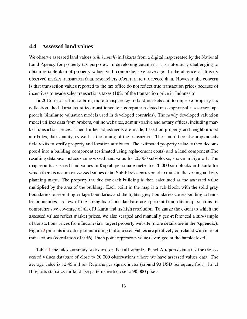
In 2015, in an effort to bring more transparency to land markets and to improve property taxcollection, the Jakarta tax office transitioned to a computer-assisted mass appraisal assessment ap-proach (similar to valuation models used in developed countries). The newly developed valuationmodel utilizes data from brokers, online websites, administrative and notary offices, including mar-ket transaction prices. Then further adjustments are made, based on property and neighborhoodattributes, data quality, as well as the timing of the transaction. The land office also implementsfield visits to verify property and location attributes. The estimated property value is then decom-posed into a building component (estimated using replacement costs) and a land component.Theresulting database includes an assessed land value for 20,000 sub-blocks, shown in Figure 1. Themap reports assessed land values in Rupiah per square meter for 20,000 sub-blocks in Jakarta forwhich there is accurate assessed values data. Sub-blocks correspond to units in the zoning and cityplanning maps. The property tax due for each building is then calculated as the assessed valuemultiplied by the area of the building. Each point in the map is a sub-block, with the solid grayboundaries representing village boundaries and the lighter grey boundaries corresponding to ham-let boundaries. A few of the strengths of our database are apparent from this map, such as itscomprehensive coverage of all of Jakarta and its high resolution. To gauge the extent to which theassessed values reflect market prices, we also scraped and manually geo-referenced a sub-sampleof transactions prices from Indonesia’s largest property website (more details are in the Appendix).Figure 2 presents a scatter plot indicating that assessed values are positively correlated with markettransactions (correlation of 0.56). Each point represents values averaged at the hamlet level.

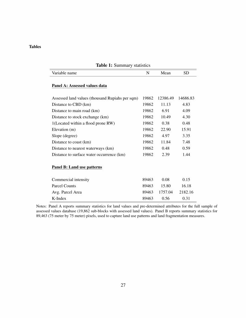
Table 1 includes summary statistics for the full sample. Panel A reports statistics for the as-sessed values database of close to 20,000 observations where we have assessed values data. Theaverage value is 12.45 million Rupiahs per square meter (around 93 USD per square foot). PanelB reports statistics for land use patterns with close to 90,000 pixels.

13

5 Empirical framework

We estimate variations of the following estimating equation:

Yi j = α +β1(KIPi j)+ γXi j +δ j + εi j (1)

where Yi j is the outcome for unit i in location j. The key regressor, 1(KIP), is a dummy equal to 1 ifi is located in a KIP treated area, according to our policy maps. Additionally, Xi j represents a vectorof pre-determined controls, δ j is a village (or hamlet) fixed effect,16 and εi j is an idiosyncratic errorterm. Our outcomes include assessed land values (where the unit of analysis is a sub-block in theassessed values database) and land use patterns (where the unit of analysis is a pixel).

The parameter of interest is β , which captures the long-term impacts of KIP, comparing treatedareas relative to non-treated areas. One major threat is that β is biased downwards because KIPtargeted low quality informal settlements. To circumvent the concern that β is identified fromcomparing slums to formal settlements, we restrict our sample to historical kampung’s that existedbefore KIP but were never treated (see Section 4.2).

Next, we implement a boundary discontinuity design comparing observations located on eitherside of KIP policy boundaries. The identification assumption is that unobserved determinants donot change differentially around the boundaries, conditional on the controls. The strength of thisstrategy is that we can restrict the sample to narrow distance bands (within 200 meters), whichholds constant many potential unobserved determinants of land values. We include boundary fixedeffects and quadratic distance controls to KIP boundaries; the results are robust to other types ofdistance controls (e.g. logs).

Additionally, we perform a number of tests to address several concerns with the boundarydiscontinuity design. First, the results may be too local and not representative of the rest of Jakarta.In particular, the differences across the boundaries may reflect a reshuffling of development activityacross the boundaries. We address this by also presenting a full sample analysis that covers all ofJakarta to assess how representative the boundary discontinuity estimates are. Second, there couldbe spillover and contamination effects across the boundaries. To address this, we present estimates

16The primary administrative units in Indonesia are districts (kabupaten), sub-districts (kecamatan), villages (kelu-rahan), hamlets (Rukun Warga, RW), and block groups (Rukun Tetangga, RT). Our empirical analysis will focusmostly on villages or hamlets. As a reference, villages have an average area of 2.5 square kilometers, and are com-parable to Census tracts in the US. Hamlets have an average area of 0.24 square kilometers and are comparable tocensus block groups.

14

that span multiple distance bands (up to 1000 meters). To the extent that access to KIP-relatedamenities declines with distance, the localized spillover effects should also exhibit spatial decaypatterns (?).

In all of our specifications, we control for location-specific natural advantage through a seriesof variables capturing access and geography. Specifically, we control for distance, in logs, from theheadquarters of the Indonesia Stock Exchange, from the National Monument in Merdeka Square(which we interpret as the city center) and from a main road. An important dimension of naturaladvantage in Jakarta is flood proneness, which played a significant role in the city’s settlementpatterns. We account for it in multiple ways: we control for distance, in logs, from the coast,from waterways and from any permanent or semi-permanent water body; moreover, we includea binary indicator for whether a hamlet is flood prone, according to flood information reported inOpenstreetmap. Finally, we account for local topography by including slope and elevation controls.All of our data sources are documented in the Appendix.

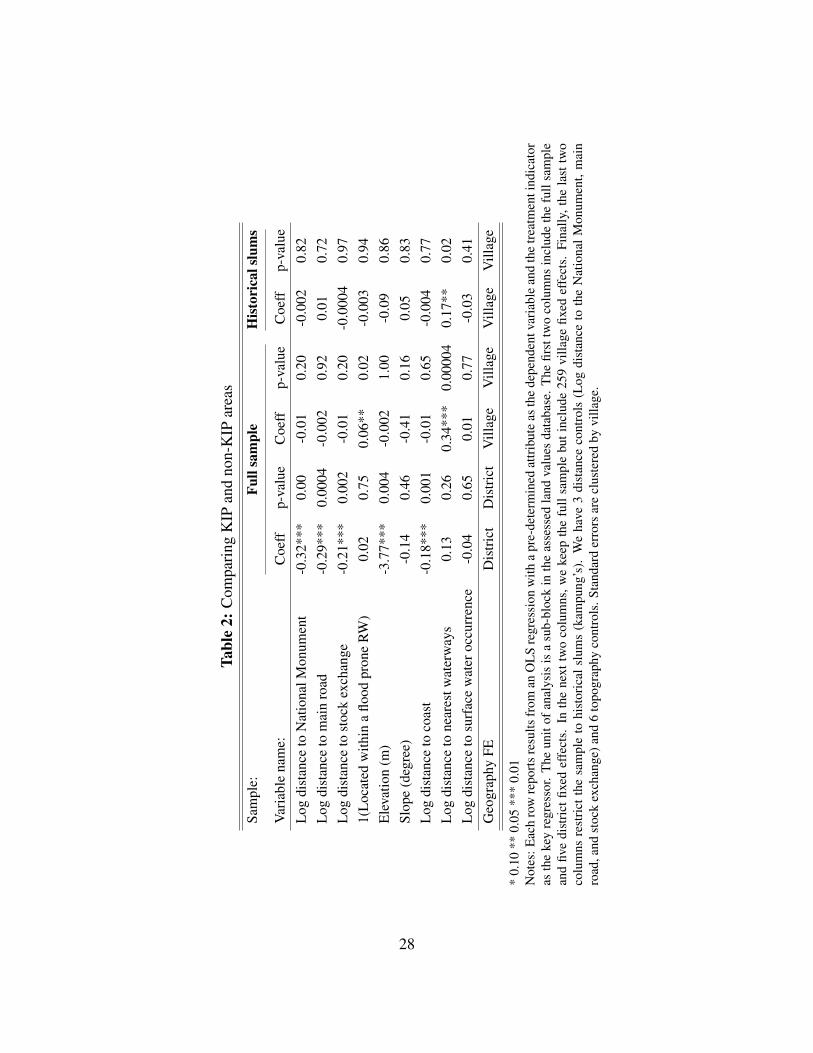
As a preliminary step, Table 2 presents regressions to assess how comparable KIP and non-KIPareas are. Each pair of cells reports the coefficient and p-value from a regression of attributes on thetreatment dummy and district or village fixed effects, with standard errors clustered at the villagelevel. The results are similar if we include hamlet fixed effects, or if we cluster standard errors atthe hamlet level. The pre-determined attributes, Xi j, include distance and topographic controls.

The first four columns include the full sample, comparing treated to non-treated areas. Wefirst report differences using five district fixed effects. As expected, KIP areas are significantlydifferent from non-KIP areas. Reassuringly, the distance and topography attributes are relativelycomparable, once we include village fixed effects. Two coefficients remain significant at the 5%level. Within a village, KIP areas are 6 percent more likely to be in flood prone hamlets and 34%further from waterways (canals that help mitigate flooding). The first difference becomes insignif-icant when we only include historical slums. For the latter, the difference is halved: KIP areas are17% further away from waterways. If anything, places that are farther from waterways have higherland values (perhaps because they are less flood prone). This suggests that this difference wouldbias against finding lower assessed land values.

15

6 Results

6.1 Effect of KIP on land values

Table 3 presents our main results for the relationship between KIP and assessed land values.Columns 1 to 3 include the full sample, with district, village, and hamlet fixed effects, respec-tively. Columns 4 and 5 restrict the sample to historical slums only. In this smaller sample, weonly have the power to include village fixed effects. Standard errors are clustered at the villagelevel.

Column 1 shows that KIP areas have 31% lower land values compared to other areas in thesame district. This difference becomes smaller (23%) once we include village fixed effects, in linewith the concern discussed above that KIP targeted lower quality locations. This 23% effect isidentified from comparing KIP and non-KIP locations within the same village.

Column 3 shows that after including 2060 hamlet (Rukun Warga, RW) fixed effects, the differ-ence reduces to 11% and remains statistically significant at the 1% level. There are 304 hamletswith within-hamlet variation in treatment status.

Columns 4 and 5 report smaller differences once we restrict the sample to historical slumsonly. One concern from the full sample analysis is that KIP selected slums only and the lowerland values are driven by pre-treatment differences between slums and non-slums. The historicalslums sample only includes kampung’s that existed before 1969. The effects on land values are-21% with district fixed effects and -12% with village fixed effects. Column 5 is identified from128 villages (out of 196) that have within-village variation in treatment status. In the rest of theempirical analysis, the specifications in columns 3 and 5 will be our baseline ones, respectively,for the full sample and historical slums sample regressions.

Next, column 6 further probes program selection concerns by examining whether the effects arelarger for the earlier waves. We report results for three separate treatment dummies (correspondingto the three five year plans). Our estimates suggest the effects are -13% for the first wave, -9% forthe second wave, and -14% for the third wave, with overlapping confidence intervals. Since KIPprioritized slums in worse conditions first, if the estimated differences are due to selection bias, theimpacts on land values should be larger for the earlier waves.

Taken together, the results in Table 3 indicate that, in the long run, KIP areas have 11 to 12percent lower assessed land values. In particular, it is reassuring that the magnitudes are similar inthe full sample with hamlet fixed effects (column 3) and in the historical slums sample with village

16

fixed effects (column 5). The 12 percent effect in column 5 is large, translating into an aggregateeffect of $11 billion US dollars.17

Boundary Discontinuity. Table 4 presents estimates from the boundary discontinuity design.Columns 1 to 3 include observations within 500, 300, and 200 meters, respectively, of the KIPprogram boundary. As discussed in Section 4.1, we only include boundary segments where obser-vations in the control group are not “contaminated” by treated areas that are nearby.

Once again, we find similar effect sizes with KIP areas having 13 to 15 percent lower landvalues. The boundary discontinuity design estimate is identified by comparing observations withinnarrow distance bands, but fall on a treated versus control side of the boundary. The main assump-tion is that unobserved determinants of land values should be similar close to the boundaries. Table1 in the Appendix shows that the pre-determined attributes are similar for KIP and non-KIP areasin the boundary discontinuity sample (similar to Table 2 discussed above). There is a potentialconcern that KIP boundaries are merely administrative boundaries, so that effects estimated froma boundary discontinuity design are driven by differences across administrative units. Importantly,we verified that the boundaries in our sample do not merely represent administrative boundaries.In particular, the neighborhood boundaries are pre-determined because these largely depend onadministrative boundaries defined before KIP; in fact, many of these neighborhood units wereintroduced by the Japanese during World War II.18

One concern that arises with the boundary discontinuity sample is contamination or spilloversbetween treatment and control areas. The stability of the estimates across the buffer distancessuggest limited evidence of spatial externalities due to KIP. Moreover, since most externalities willplausibly affect land values in the same way as the direct KIP effect, spatial externalities will likelybias against us finding any effect.

Next, we further explore potential spatial externalities by examining whether the effect onland values exhibits any spatial decay, as we move away from the KIP boundaries (?). Localizedexternalities provide an economic motivation for slum upgrading policies. Residents of nearby

17The average assessed value for historical slums is 12 million Rupiahs per square meter (around US$89 per squarefoot), translating into an effect size of 1.4 million Rupiahs per square meter, or US$11 per square foot (at an exchangerate of 13,371 Rupiahs to US dollars). We obtain the aggregate effect by multiplying by the total area under KIP, 100million square meters (10,000 hectares). Note that this back-of-the-envelope exercise does not account for potentialdifferences in building height. The total effect could be larger if we also account for potential effects on the numberof floors built.

18During the occupation in World War II, the Japanese army introduced the system of Rukun Warga (RW hamlets,smaller than villages) and Rukun Tetangga (RT blocks, smaller than hamlets) for security purposes.

17

non-slum areas are often concerned over negative spillovers stemming from unsanitary living con-ditions and depressed public and private investment in slums.

We estimate spatial decay patterns by exploring heterogeneous effects by distance bands. Werepeat the same specifications as Table 3, but the omitted group is now the treatment group andthe key regressors include indicators for areas outside of KIP and within 100 meter distance bands.We start with 0 to 100 meters, and include up to 10 distance bands (900 to 1000 meters). Wedrop observations beyond 1000 meters.19 Figure 5 plots the effects by distance bands and the95% confidence intervals, confirming the lack of spatial decay patterns. The full set of regressionresults is reported in Table 2. All columns indicate no significant spatial decay pattern. In columns1 and 2, the 95% confidence intervals are quite stable and overlap with each other. In column 3,with hamlet fixed effects, the coefficients beyond the 500 meters bands are not significant becausethere is little within-hamlet variation beyond 500 meters.20 The conclusions are similar using thehistorical sample in columns 4 and 5.

Bias from Land Values Assessment. Next, we consider the possibility that the negative land val-ues are driven by differences in the quality of the assessed land values. First, to the extent that themeasurement error is smooth across KIP boundaries, it is unlikely that the boundary discontinuityestimates are driven by measurement error.

Nevertheless, one concern is that KIP areas are more likely to be informal today, and propertydata for informal settlements are less likely to be reported. Table 3 in the Appendix investigateswhether KIP areas are less likely to have assessed values. The unit of analysis is a 75 by 75 meterpixel and the dependent variable is whether we observe an assessed value for the pixel. In contrastto concerns that KIP areas are less likely to be included the assessed values database, we actuallyfind a positive coefficient on the treatment dummy. Column 1 includes the full sample with hamletfixed effects and column 2 restricts the sample to historical slums only, with village fixed effects.

Furthermore, we show in Table 4 in the Appendix that the negative impact on land valuessurvives if we drop areas that are more likely to be informal. This is a difficult exercise becausethere is no direct measure of informality. As a way around this, we assume that areas with greaterland fragmentation (as defined in Section 4) are more likely to be informal. We show that ourresults survive even when we drop pixels in the top quartile of our proxies of land fragmentation.This reduces the concern that our results are driven by measurement error that is correlated with19The average village has an area of 2.5 square kilometer, implying an equivalent area radius of 892 meters.20The average hamlet has an area of 243,156 square meters, implying an equivalent area radius of 278 meters.

18

informality and the treatment indicator.

6.2 Effect of KIP on land use patterns

Next, we discuss our results for land use patterns. In our analysis of spatial development patterns,our units of observation are 75 meter by 75 meter pixels that we obtain by superimposing a gridover the territory of Jakarta. This approach ensures that the units are comparable in size andshape, while the arbitrariness of the grid minimizes concerns of endogeneity with respect to theprogram’s boundaries. The size of each pixel (approximately 5600 square meters) is comparableto the amount of contiguous land that needs to be assembled for an average high-rise developmentproject in Jakarta, based on reports from the Jakarta City Planning Agency.

Commercial Intensity. Table 5 presents estimates of the effect of KIP on commercial devel-opment activity. The unit of analysis is a 75 meter by 75 meter pixel. The dependent variable isthe share of area in that pixel corresponding to commercial development. The regressor is 1 if thepixel is located in KIP. Standard errors are clustered by village.

Across the columns, we consistently find that KIP areas have lower commercial intensity. Col-umn 1 reports a negative 4 percentage point (p.p.) effect using the historical slums sample andvillage fixed effects (analogous to column 5 of Table 3). As a benchmark, the sample mean is 0.06and the standard deviation is 0.12.

One concern is selection into development: we could be comparing locations with greater po-tential for commercial development (such as locations zoned for commercial and locations withgood accessibility) and locations with less potential for commercial activity. To address this se-lection concern, column 2 reports a negative 6 p.p. effect, restricting the sample to pixels that arezoned for commercial development. As another proxy for development potential, we also consid-ered pixels that are within 1000 meters of a predetermined road and find similar results. Next,column 3 reports a negative 5 p.p. effect using the 200 meter boundary discontinuity specification.In order to address concerns that the historical slums or boundary discontinuity samples are local-ized, Table 5 in the Appendix shows that our conclusions for land use patterns remain the same ifwe use the full sample and include hamlet fixed effects.

Land Fragmentation. In Table 6, we explore the impact of KIP on fragmentation, measuredthrough the three indexes discussed in Section 4: parcel count (columns 1 and 2), average parcel

19

area (columns 3 and 4) and the K fragmentation index (columns 5 and 6). For each index, we reportestimation results in the historical sample (odd columns) and the 200 meter boundary discontinuityspecification (even columns). Besides our standard set of distance and geography controls, we alsocontrol for the total log length of roads in the pixel, as the presence of road intersections maymechanically increase observed fragmentation.

The KIP treatment appears to be associated to a higher degree of land fragmentation, acrossour range of indexes and specifications. KIP areas have on average 9 to 13 more parcels per pixel.Additionally, the average parcel area is smaller by approximately 560 square meters (about 20% ofthe area of a pixel) to 960 square meters. These are sizable impacts, considering that the averageparcel count and area in control pixels is, respectively, 19 parcels and 1280 square meters. Impactson the K index are best understood in standardized terms: relative to control pixels, KIP pixels aremore fragmented by roughly 2/5ths to 2/3rds of a standard deviation of the K index. As a reference,the average value of the K index is 0.5 in the control sample. Table 5 in the Appendix shows thatour conclusions are unchanged when using the full sample.

In order to appreciate to what extent land fragmentation contributes to the negative impact ofKIP on land values, we can relate the results above to the impact of fragmentation on land valueswithin KIP areas. Column 1 of Table 7 shows that one additional parcel per pixel is associated toa 1% decline in land values in KIP areas; a parcel size smaller by 100 square meters leads to a1.59% decline; and a 0.1 increase in the K index leads to a 10.2% decline. Benchmarked to thesefigures, fragmentation as captured by our three indicators explain 72%, 74% and 102% of the total12% effect.

6.3 Heterogeneity analysis

Our next exercise is to investigate where the effects are the largest. We first show that the effects onland values and commercial development are larger in the city center than the periphery. We definethe center of the city as the National Monument, which is mentioned in many planning documentsas a major landmark and a hub for the city. Our conclusions are similar if we use other definitionsof the city center.

Table 8 extends our most saturated specification with the full sample (column 3 of Table 3),dividing Jakarta into terciles according to the distance to the National Monument (central, middle,periphery) and interacting these tercile indicators with the treatment indicator. The omitted group

20

is the periphery. We report heterogeneous effects for land values (column 1), commercial intensity(column 2), and land fragmentation (K-index, column 3).

Column 1 demonstrates that the average land value in central KIP areas is 9% lower than theaverage land value for non-KIP areas in the center. The coefficient on the interaction term is largeand statistically significant (-0.144) but the direct effect is insignificant. The treatment effect is alsolarge and significant for the middle tercile (10.8%), but the effect at the periphery is small (-0.015)and insignificant. Since the program was implemented so long ago, KIP areas are concentratedin central areas (67% of the 10,000 hectares), with 27% in the middle, and 6% in the periphery.We can repeat our aggregation exercise to calculate the implied total opportunity cost of land use,accounting for the heterogeneity in KIP impacts and coverage across different parts of the city.Our calculations suggest the opportunity cost of land use is $9.3 billion in the center, $2 billion inthe middle, and $35 million in the periphery.

Column 2 shows a similar pattern for commercial development. Central, non-KIP areas aremore likely to be commercial (3.9 p.p.), but central, KIP areas are less likely to be commercial(-4.4 p.p.), implying a treatment effect of -8.3 p.p. In the medium tercile, the treatment effect is-3.7 p.p. and in the periphery, the effect is -3.3 p.p..

Overall, this pattern of heterogeneous effects is consistent with the interpretation of delayedformalization in KIP areas. Central areas, that have greater market potential, are the ones associatedwith a larger opportunity cost of land use and will tend to be formalized earlier, leading to a largerobserved gap in land values. Column 3 shows the effects on land fragmentation are stable across thethree terciles. This could be because the impact on land fragmentation is confounded by oppositeforces:on the one hand, greater population density in more central areas may be associated withgreater land fragmentation; on the other, greater market potential in central areas will induce moreformalization and land consolidation, resulting in a lower degree of fragmentation.

Our second heterogeneous effects exercise relates to KIP policy components. In Table 9 weshow that the effects of KIP on land values are not differential by the three main KIP policycomponents - roads, sanitation, and buildings (health centers and schools). We observe the locationand type of KIP investments from the policy maps. For each assessed land value observation, wequantify the amount of KIP investments located within a 500 meter buffer, for observations in KIPand non-KIP areas. This allows for the possibility that non-KIP areas are also able to access KIPpolicy investments. To quantify road investments, we calculate the length of roads built by KIPwithin 500 meters of each observation. To quantify the prevalence of sanitation facilities and public

21

buildings, we count the number of facilities within 500 meters. Additionally, we de-meaned thesethree measures of KIP investments so that the coefficient on the treatment indicator corresponds tothe average treatment effect (evaluated at the average of these three investment measures). Eachcolumn in this table follows the specification of the corresponding column in Table 3. In column 1,we find that roads have a positive effect on land values (0.04 coefficient), but this effect disappearsonce we add finer fixed effects. Besides roads, we do not find differential treatment effects by thetype of investment.

The lack of heterogeneity in effects by policy investments is consistent with the notion thatdifferences in initial public investment levels may have equalized across KIP and non-KIP areasby now. This could be because most of the initial investments have plausibly depreciated over threeto four decades. We corroborate this in Table 6, where the dependent variable measures distanceto the closest public amenity (including KIP-related investments such as schools, and other publicamenities such as hospitals, police stations, and bus stops.

Overall, we find small and largely insignificant differences in access to public amenities. KIPareas are on average 5% further away from hospitals, but this difference only amounts to 63 meters.The confidence intervals in levels are all small and relatively narrow around zero. The dependentvariable means show that average distance to schools, hospitals, police stations and bus stops arerespectively 520 meters, 1.2 kilometers, 2 kilometers, and 1.6 kilometers.

7 Policy implications

In Section 5 we calculate an aggregate impact of KIP on land values of approximately US$11billion, which we interpret as the long-run costs of the program.21 In this Section, we assess themagnitude of this estimated impact and provide several bounding exercises in order to evaluate thepolicy implications of our findings.

Our first exercise relates to the question of whether the program had an ex ante net presentvalue. As discussed in Section 3, in this setting there are person-based benefits that are not capital-ized into local land values - for instance, original beneficiaries may have moved and invested their

21This figure results from a simple aggregation of the program’s estimated impact on land values over KIP treatedareas and does not account for how the spatial patterns of development were distorted by the program. In futurework we will refine this aggregation exploiting heterogeneity in development activity across different parts of thecity.

22

accumulated human capital elsewhere. As a result, our estimates of an aggregate negative impactof US$11 billion are not interpretable as a welfare loss. This figure should be interpreted as anaggregate long-run cost, that should be weighed against the program’s benefits in order to assessits cost/benefit balance. Such benefits will include not only the returns from improved health andeducation resulting from physical KIP investments, but also, more broadly, the value of living in arelatively central location with less of a risk of eviction or displacement relative to slum dwellersin non-KIP areas. These impacts are inherently difficult to quantify and to estimate causally due toa lack of data and the endogenous mobility of original program recipients.22

While we cannot provide estimates of the net present value of the program, we perform abounding exercise to assess how large these person-based benefits need to be for the programto have a positive net present value. Our calculation involves two steps. First, we express theestimated aggregate cost of US$11 billion in per-capita terms, dividing it by the number of originalrecipients - 5 million people according to KIP reports (?).23 Assuming an average household sizeof 4 people (a figure derived from a field survey we conducted in 2016), the cost per originalbeneficiary household amounts to US$8,800. The second step is to account for the time value ofmoney and compute the present value of this figure at the time of the program’s implementation.We take 1975 as a reference year. Applying a discount rate of 5% as used in the literature (?), thepresent value per beneficiary household in 1975 was US$1,190, a figure that is roughly twice aslarge as their annual household income at the time (US$600, ?). If KIP benefits per beneficiaryhousehold were greater than this figure, the program had an ex ante a positive net present value.

In our second exercise we adopt the perspective of a policy maker in a city that has already im-plemented slum upgrading and that is facing the long-run misallocation costs that we highlight. Weconsider the option of realizing the estimated US$11 billion opportunity cost by redeveloping KIPareas and redistributing the surplus to current residents. The process of clearing slums for rede-velopment is a contentious and politically charged one, involving important equity considerationsrelated to the displacement and compensation of slum dwellers. Acknowledging these considera-tions, we offer a range of estimates of the maximum possible compensation per individual residentthat could be provided, assuming the entire surplus from redevelopment were allocated to dis-placed residents. This calculation involves dividing the aggregate US$11 billion by the number of

22Although surveys were conducted for purposes of impact evaluation (?). they cannot provide definitive estimates onthe program’s impact on its beneficiaries because of their cross-sectional nature and limited power (see Section 2).

23This figure only accounts for the original recipients, neglecting migrants and subsequent generations that plausiblyalso benefited from KIP improvements. Therefore, our calculation should be thought of as conservative.

23

current residents of KIP areas. Given the lack of granular data on population, we provide a range ofestimates of the number of current residents based on different population density assumptions.24

Assuming a density of 300 people per hectare, current residents of KIP areas amount to 3 millionpeople, or 750,000 households. The surplus available per displaced household is thus US$14,700.We can benchmark this figure to the current annual household income in kampung’s (US$3,660),based on our 2016 field survey. The implied compensation per household is approximately 4 timesthe annual household income. Under alternative assumptions of a density of 500 or 800 people perhectare, this compensation amounts respectively to 2.4 and 1.5 times the annual household income.

A question then arises on whether this is amount is sufficient compensation for displacement.While the literature provides no explicit estimates of displacement costs for slum households, theevidence from programs relocating slum dwellers into public housing suggests that such costs areprobably sizable, especially for residents of slums in the center of cities. For instance, ? considerone such program in Ahmedabad, India, and find that the majority of program recipients hadgiven up subsidized housing in the city’s periphery and moved back to the slums. By revealedpreferences, this suggests that the non-monetary costs of relocation are likely to be large. Suchcosts plausibly include not only increased commuting times but also the potential destruction ofsocial capital and informal insurance networks that displacement entails.

Overall, our bounding exercise suggests that slum redevelopment with compensation of currentresidents may be a viable option only when the opportunity cost of land is high relative to thenumber of current residents. The relative dynamics of land prices and population will determine atwhich stage in the city’s evolution this point is reached.

8 Conclusion

As cities in developing countries prepare to accommodate an unprecedented wave of urban expan-sion, policy makers are debating different policy approaches to facilitate the massive urbanizationflows. In this paper, we provide novel causal evidence of the long-term impacts of the world’slargest scale slum upgrading program, the Kampung Improvement Program, in the city of Jakarta.Our setting is unique in that we have granular data on a city that has recently started formalizing,over 40 years from the implementation of the program.

24The Jakarta Department of Housing categorizes slums as low density (less than 300 people per hectare), mediumdensity (300-800 people per hectare) or high density (over 800 people per hectare).

24

Across empirical exercises and robustness checks, we consistently find that KIP areas have 12%lower land values. KIP areas also display less commercial activity and greater land fragmentation.These findings suggest that the program slowed down the formalization process, resulting in anunintended long-run distortionary cost. Aggregating over KIP treated areas, this opportunity costof land use amounts to US$11 billion.

We complement our analysis with several bounding exercises aimed at informing policy. First,we consider the tradeoff between the program’s benefits and its long-run costs. We estimate thatit would take benefits greater than twice the annual household income of original recipients forthe program to have an ex ante positive net present value. Second, we evaluate the maximumpossible compensation per current KIP resident in a scenario in which KIP neighborhoods wereredeveloped. This implied compensation ranges from 1.5 to 4 times the current residents’ annualhousehold income. This figure is likely to become larger over time as land values grow moresteeply than population, so that redevelopment may become more likely in the future.

The governments of many countries today are considering slum upgrading. Our findings canhelp inform their policy decisions in a number of ways. One general lesson is that slum upgradingentails long-run distortionary costs, and that such costs should be weighed against a program’sbenefits. As these distortionary costs will manifest themselves once a city starts formalizing, thebalance between costs and benefits will partly depend on the timing of the implementation of theprogram and the stage or development that a city is in. For a city comparable to Jakarta in 1969,slum upgrading may be an attractive policy option, since these long-run costs will materialize farin the future. On the other hand, for a city that has already started formalizing, the opportunitycost of land use may already be too high for slum upgrading to have a positive net present value.Another policy implication is that slum upgrading may be more successful if complemented byother measures, aimed at facilitating formalization and the development of well-functioning landmarkets. In future work, it will be interesting to elaborate on these tradeoffs further and developa stylized model to present scenarios in which slum upgrading can be more or less attractive thanother policy counterfactuals.

Another direction for future work is to enrich the empirical analysis with more outcomes. Inan ongoing data collection effort, we are combining imagery from Google StreetView and fromfield visits in order to collect a representative sample of urban views. Through a process of manualclassification, we are coding a number of attributes of the built environment from each of theseimages. Such attributes include building heights - that will allow us to shed more light on the

25

quantity margin of development activity - but also a broader set of building characteristics that wecould use to proxy for the presence of current slums, which are inherently hard to detect due toa lack of consistent definitions. Furthermore, disaggregated population counts and richer data oncurrent amenities will also allow us to gain a deeper understanding of the program’s impacts.

26

Tables

Table 1: Summary statistics

Variable name N Mean SD

Panel A: Assessed values data

Assessed land values (thousand Rupiahs per sqm) 19862 12386.49 14686.83Distance to CBD (km) 19862 11.13 4.83Distance to main road (km) 19862 6.91 4.09Distance to stock exchange (km) 19862 10.49 4.301(Located within a flood prone RW) 19862 0.38 0.48Elevation (m) 19862 22.90 15.91Slope (degree) 19862 4.97 3.35Distance to coast (km) 19862 11.84 7.48Distance to nearest waterways (km) 19862 0.48 0.59Distance to surface water occurrence (km) 19862 2.39 1.44

Panel B: Land use patterns

Commercial intensity 89463 0.08 0.15Parcel Counts 89463 15.80 16.18Avg. Parcel Area 89463 1757.04 2182.16K-Index 89463 0.56 0.31

Notes: Panel A reports summary statistics for land values and pre-determined attributes for the full sample ofassessed values database (19,862 sub-blocks with assessed land values). Panel B reports summary statistics for89,463 (75 meter by 75 meter) pixels, used to capture land use patterns and land fragmentation measures.

27

Tabl

e2:

Com

pari

ngK

IPan

dno

n-K

IPar

eas

Sam

ple:

Full

sam

ple

His

tori

cals

lum

s

Var

iabl

ena

me:

Coe

ffp-

valu

eC

oeff

p-va

lue

Coe

ffp-

valu

eL

ogdi

stan

ceto

Nat

iona

lMon

umen

t-0

.32*

**0.

00-0

.01

0.20

-0.0

020.

82L

ogdi

stan

ceto

mai

nro

ad-0

.29*

**0.

0004

-0.0

020.

920.

010.

72L

ogdi

stan

ceto

stoc

kex

chan

ge-0

.21*

**0.

002

-0.0

10.

20-0

.000

40.

971(

Loc

ated

with

ina

flood

pron

eR

W)

0.02

0.75

0.06

**0.

02-0

.003

0.94

Ele

vatio

n(m

)-3

.77*

**0.

004

-0.0

021.

00-0

.09

0.86

Slop

e(d

egre

e)-0

.14

0.46

-0.4

10.

160.

050.

83L

ogdi

stan

ceto

coas

t-0

.18*

**0.

001

-0.0

10.

65-0

.004

0.77

Log

dist

ance

tone

ares

twat

erw

ays

0.13

0.26

0.34

***

0.00

004

0.17

**0.

02L

ogdi

stan

ceto

surf

ace

wat

eroc

curr

ence

-0.0

40.

650.

010.

77-0

.03

0.41

Geo

grap

hyFE

Dis

tric

tD

istr

ict

Vill

age

Vill

age

Vill

age

Vill

age

*0.

10**

0.05

***

0.01

Not

es:E

ach

row

repo

rts

resu

ltsfr

oman

OL

Sre

gres

sion

with

apr

e-de

term

ined

attr

ibut

eas

the

depe

nden

tvar

iabl

ean

dth

etr

eatm

enti

ndic

ator

asth

eke

yre

gres

sor.

The

unit

ofan

alys

isis

asu

b-bl

ock

inth

eas

sess

edla

ndva

lues

data

base

.T

hefir

sttw

oco

lum

nsin

clud

eth

efu

llsa

mpl

ean

dfiv

edi

stri

ctfix

edef

fect

s.In

the

next

two

colu

mns

,we

keep

the

full

sam

ple

buti

nclu

de25

9vi

llage

fixed

effe

cts.

Fina

lly,t

hela

sttw

oco

lum

nsre

stri

ctth

esa

mpl

eto

hist

oric

alsl

ums

(kam

pung

’s).

We

have

3di

stan

ceco

ntro

ls(L

ogdi

stan

ceto

the

Nat

iona

lMon

umen

t,m

ain

road

,and

stoc

kex

chan

ge)a

nd6

topo

grap

hyco

ntro

ls.S

tand

ard

erro

rsar

ecl

uste

red

byvi

llage

.

28

Table 3: Effect of KIP on land values

Dependent variable: Log land values

Sample: Full sample Historical slums

(1) (2) (3) (4) (5) (6)KIP -0.31*** -0.23*** -0.11*** -0.21*** -0.12***

(0.07) (0.04) (0.03) (0.06) (0.05)KIP I (1969-1974) -0.13

(0.09)KIP II (1974-1979) -0.09

(0.06)KIP III (1979-1984) -0.14*

(0.07)N 19862 19862 19862 3147 3147 3147R-Squared 0.54 0.75 0.85 0.52 0.73 0.73Distance Y Y Y Y Y YTopography Y Y Y Y Y YGeography FE District Village Hamlet District Village Village

* 0.10 ** 0.05 *** 0.01Notes: The table reports results from an OLS regression with the log of assessed land values as the dependentvariable (rupiahs per square meter). The key regressor is the treatment indicator. The unit of analysis is a sub-blockin the assessed land values database. The estimation sample for columns 1 to 3 consists of 19,862 sub-blocks.Column 1 includes 5 district fixed effects. Column 2 includes 259 village fixed effects. Column 3 includes 2060hamlet fixed effects. In addition, all columns include 9 attributes (defined in Table 2) as controls. Columns 4 and5 reports the specifications of columns 1 and 2, but restrict the sample to observations in historical slums only.Column 6 reports the specification of column 5, with the key regressors being three dummies corresponding tothe three different KIP pelita (five-year plan) waves. Standard errors are clustered by village.

29

Table 4: Effect of KIP on land values: Boundary discontinuity design

Dependent variable: Log land values

Sample: 500m 300m 200m(1) (2) (3)

1(KIP) -0.15*** -0.15*** -0.13**(0.05) (0.05) (0.06)

N 2820 2039 1317R-Squared 0.81 0.81 0.81Distance to KIP boundary Y Y YDistance Y Y YTopography Y Y YKIP Boundary FE Y Y Y

* 0.10 ** 0.05 *** 0.01Notes: This table reports results from an OLS regression with the log of assessed land values as the dependentvariable. The key regressor is the treatment indicator. The unit of analysis is a sub-block in the assessed land valuesdatabase. Column 1 reports results with 123 KIP boundary fixed effects, 9 distance and topography attributes, anda control for distance to a KIP policy boundary for a sample of observations within 500 meters of a KIP boundary.Columns 2 and 3 restrict the sample to properties within 300 meters and 200 meters of a KIP boundary. Standarderrors are clustered by the 123 KIP boundaries in our analysis.

30

Table 5: Effect of KIP on land use: Commercial intensity

Dependent variable: Commercial intensity

Sample: Historical slums BDD 200m

(1) (2) (3)1(KIP) -0.04*** -0.06*** -0.05***

(0.01) (0.02) (0.01)N 11015 1553 5412R-squared 0.20 0.31 0.30Distance Y Y YTopography Y Y YZoned Commercial N Y NDistance to KIP boundary N N YGeography FE Village Village KIP boundary

* 0.10 ** 0.05 *** 0.01Notes: This table reports results from an OLS regression with the share of commercial development within apixel as the dependent variable. The key regressor is the treatment indicator. The unit of analysis is a 75m×75mpixel. Column 1 reports results using the historical sample with village fixed effects, distance, and topographyattributes. Column 2 restricts the sample to observations zoned for commercial development. Column 3 reports theboundary discontinuity design specification with observations within 200 meters from a KIP boundary, controllingfor distance to the boundary. Standard errors are clustered by village (columns 1 and 2), and by KIP boundaries(column 3).

31

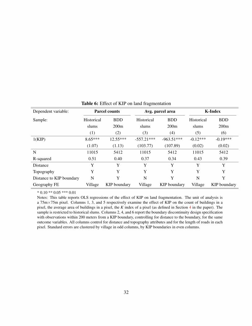
Table 6: Effect of KIP on land fragmentation

Dependent variable: Parcel counts Avg. parcel area K-Index

Sample: Historical BDD Historical BDD Historical BDDslums 200m slums 200m slums 200m

(1) (2) (3) (4) (5) (6)1(KIP) 8.65*** 12.55*** -557.21*** -963.51*** -0.12*** -0.19***

(1.07) (1.13) (103.77) (107.89) (0.02) (0.02)N 11015 5412 11015 5412 11015 5412R-squared 0.51 0.40 0.37 0.34 0.43 0.39Distance Y Y Y Y Y YTopography Y Y Y Y Y YDistance to KIP boundary N Y N Y N YGeography FE Village KIP boundary Village KIP boundary Village KIP boundary

* 0.10 ** 0.05 *** 0.01Notes: This table reports OLS regressions of the effect of KIP on land fragmentation. The unit of analysis isa 75m×75m pixel. Columns 1, 3, and 5 respectively examine the effect of KIP on the count of buildings in apixel, the average area of buildings in a pixel, the K index of a pixel (as defined in Section 4 in the paper). Thesample is restricted to historical slums. Columns 2, 4, and 6 report the boundary discontinuity design specificationwith observations within 200 meters from a KIP boundary, controlling for distance to the boundary, for the sameoutcome variables. All columns control for distance and topography attributes and for the length of roads in eachpixel. Standard errors are clustered by village in odd columns, by KIP boundaries in even columns.

32

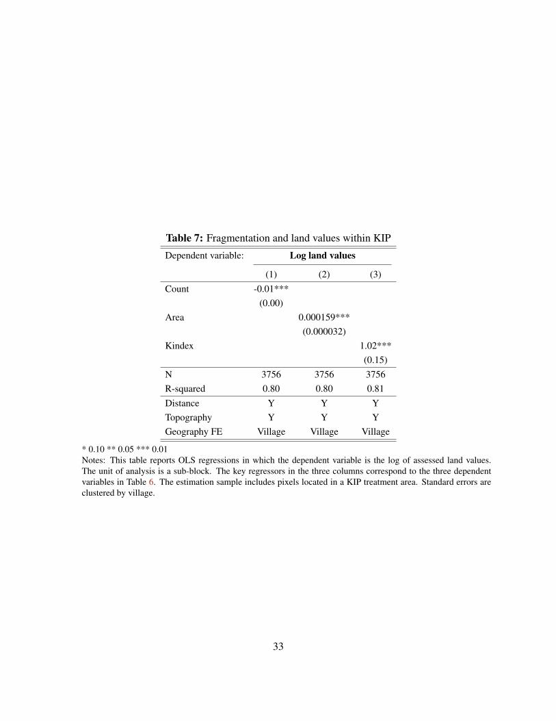
Table 7: Fragmentation and land values within KIP

Dependent variable: Log land values

(1) (2) (3)Count -0.01***

(0.00)Area 0.000159***

(0.000032)Kindex 1.02***

(0.15)N 3756 3756 3756R-squared 0.80 0.80 0.81Distance Y Y YTopography Y Y YGeography FE Village Village Village

* 0.10 ** 0.05 *** 0.01Notes: This table reports OLS regressions in which the dependent variable is the log of assessed land values.The unit of analysis is a sub-block. The key regressors in the three columns correspond to the three dependentvariables in Table 6. The estimation sample includes pixels located in a KIP treatment area. Standard errors areclustered by village.

33

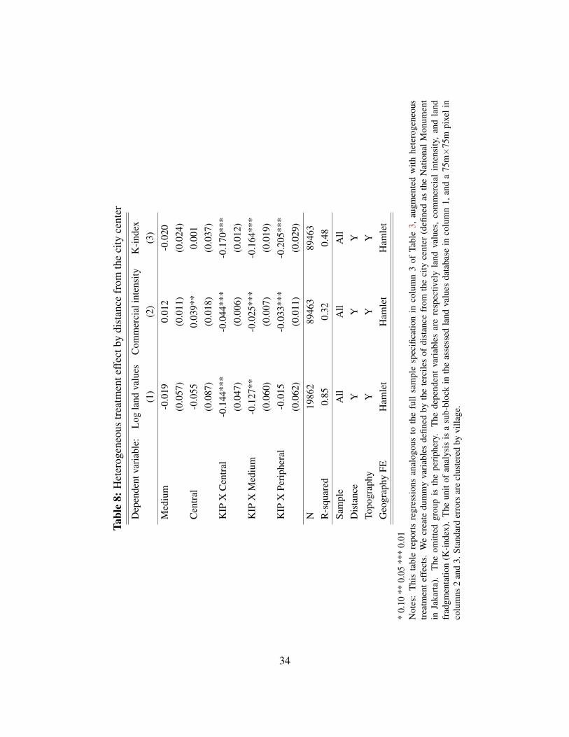
Tabl

e8:

Het

erog

eneo

ustr

eatm

ente

ffec

tby

dist

ance

from

the

city

cent

er

Dep

ende

ntva

riab

le:

Log

land

valu

esC

omm

erci

alin

tens

ityK

-ind

ex(1

)(2

)(3

)M

ediu

m-0

.019

0.01

2-0

.020

(0.0

57)

(0.0

11)

(0.0

24)

Cen

tral

-0.0

550.

039*

*0.

001

(0.0

87)

(0.0

18)

(0.0

37)

KIP

XC

entr

al-0

.144

***

-0.0

44**

*-0

.170

***

(0.0

47)

(0.0

06)

(0.0

12)

KIP

XM

ediu

m-0

.127

**-0

.025

***

-0.1

64**

*(0

.060

)(0

.007

)(0

.019

)K

IPX

Peri

pher

al-0

.015

-0.0

33**

*-0

.205

***

(0.0

62)

(0.0

11)

(0.0

29)

N19

862

8946

389

463

R-s

quar

ed0.

850.

320.

48Sa

mpl

eA

llA

llA

llD

ista

nce

YY

YTo

pogr

aphy

YY

YG

eogr

aphy

FEH

amle

tH

amle

tH

amle

t

*0.

10**

0.05

***

0.01

Not

es:

Thi

sta

ble

repo

rts

regr

essi

ons

anal

ogou

sto

the

full

sam

ple

spec

ifica

tion

inco

lum

n3

ofTa

ble

3,au

gmen

ted

with

hete

roge

neou

str

eatm

ente

ffec

ts.

We

crea

tedu

mm

yva

riab

les

defin

edby

the

terc

iles

ofdi

stan

cefr

omth

eci

tyce

nter

(defi

ned

asth

eN

atio

nalM

onum

ent

inJa

kart

a).

The

omitt

edgr

oup

isth

epe

riph

ery.

The

depe

nden

tva

riab

les

are

resp

ectiv

ely

land

valu

es,

com

mer

cial

inte

nsity

,an

dla

ndfr

adgm

enta

tion

(K-i

ndex

).T

heun

itof

anal

ysis

isa

sub-

bloc

kin

the

asse

ssed

land

valu

esda

taba

sein

colu

mn

1,an

da

75m×

75m

pixe

lin

colu

mns

2an

d3.

Stan

dard

erro

rsar

ecl

uste

red

byvi

llage

.

34

Table 9: Heterogeneous effects by KIP component

Dependent variable: Log land values

Sample: Full sample Historical slums

(1) (2) (3) (4) (5)KIP -0.22*** -0.16*** -0.11*** -0.09 -0.08

(0.07) (0.05) (0.04) (0.07) (0.05)Length of Paved Roads -0.03** -0.00 0.00 -0.02 -0.02

(0.02) (0.01) (0.01) (0.02) (0.01)Number of Sanitation Facilities 0.00 -0.01 0.00 -0.01* 0.00

(0.01) (0.01) (0.01) (0.01) (0.01)Number of Public Buildings -0.06 -0.02 0.01 0.01 0.01

(0.06) (0.02) (0.02) (0.06) (0.03)KIP X Length of Paved Roads 0.04** -0.01 -0.00 0.03 -0.01

(0.02) (0.01) (0.01) (0.02) (0.01)KIP X Number of Sanitation Facilities -0.02 0.00 -0.00 0.00 0.00

(0.01) (0.01) (0.01) (0.01) (0.01)KIP X Number of Public Buildings 0.01 0.00 0.02 -0.05 -0.01

(0.05) (0.03) (0.02) (0.06) (0.03)N 19862 19862 19862 3147 3147R-Squared 0.56 0.75 0.85 0.53 0.73Distance Y Y Y Y YTopography Y Y Y Y YGeography FE District Village Hamlet District Village

* 0.10 ** 0.05 *** 0.01Notes: Column 1 extends the full sample specification in column 3 of Table 3 to report heterogeneous treatmenteffects by the three policy components (roads, sanitation, buildings). The unit of analysis is a sub-block in theassessed land values database. The intensity of KIP policy investments is measured by length of paved roads,number of sanitation facilities, and number of public buildings within a 500 meters buffer around each observation.The KIP intensity variables have been demeaned so that the coefficient on the treatment indicator reflects theeffects when evaluated at average intensity levels. The omitted category is non-KIP areas. Standard errors areclustered by village.

35

Figures

36

Figure 1: Map of the assessed land values database

Notes: Map showing the coverage of the assessed land values database throughout Jakarta. Each shaded polygoncorresponds to a sub-block. Thick boundaries correspond to villages. Light boundaries correspond to hamlets.

37

Figure 2: Scatter plot of assessed land values and transaction prices

Correlation = 0.5614

1516

1718

19ln

(ass

esse

d va

lue,

Rp.

per

sq.

m)

14 15 16 17 18 19ln(transaction price, Rp. per sq. m)

Notes: This figure correlates the log of assessed land values and the log of transaction prices from www.brickz.id.Each point represents values averaged at the hamlet level.

38

Figure 3: KIP boundaries and historical slums

Notes: Map showing KIP boundaries (thick border) and historical slums that existed before KIP (shaded region).

39

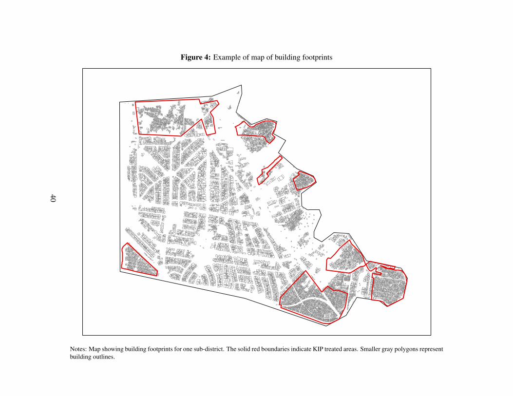
Figure 4: Example of map of building footprints

Notes: Map showing building footprints for one sub-district. The solid red boundaries indicate KIP treated areas. Smaller gray polygons representbuilding outlines.

40

Figure 5: Effect of KIP on land values: Spatial decay

−.2

−.1

0

.1

.2

.3

.4

100 200 300 400 500 600 700 800 900 1000meters

Notes: Each point corresponds to a coefficient and 95 percent confidence interval for the distance bins regressors inthe specification reported in column 5 of Table 2.

41

Appendix Tables

42

Tabl

e1:

Com

pari

ngK

IPan

dno

n-K

IPar

eas,

boun

dary

disc

ontin

uity

sam

ple

Sam

ple:

500m

300m

200m

Var

iabl

ena

me:

Coe

ffp-

valu

eC

oeff

p-va

lue

Coe

ffp-

valu

eL

ogdi

stan

ceto

CB

D0.

010.

520.

004

0.60

0.00

10.

80L

ogdi

stan

ceto

mai

nro

ad0.

04*

0.09

0.01

0.72

-0.0

020.

89L

ogdi

stan

ceto

stoc

kex

chan

ge0.

001

0.83

0.00

040.

94-0

.002

0.62

1(L

ocat

edw

ithin

aflo

odpr

one

RW

)0.

010.

880.

050.

350.

11**

0.04

Ele

vatio

n(m

)-0

.34

0.34

-0.0

20.

970.

300.

55Sl

ope

(deg

ree)

-0.6

30.

11-0

.71

0.20

-0.1

60.

49L

ogdi

stan

ceto

coas

t-0

.001

0.89

0.00

020.

980.

0003

0.95

Log

dist

ance

tone

ares

twat

erw

ays

0.25

***

0.00

10.

28**

*0.

0003

0.28

***

0.00

3L

ogdi

stan

ceto

surf

ace

wat

eroc

curr

ence

0.00

40.

890.

010.

770.

010.

57K

IPB

ound

ary

FEY

YY

YY

Y

*0.

10**

0.05

***

0.01

Not

es:T

his

tabl

ere

plic

ates

Tabl

e2,

fort

heth

ree

boun

dary

disc

ontin

uity

sam

ples

repo

rted

inTa

ble

4.

43

Table 2: Effect of KIP on land values: Spatial decay

Dependent variable: Log land values

Sample: Full sample Historical slums

Distance to KIP boundary (m) (1) (2) (3) (4) (5)[1, 100] 0.18*** 0.19*** 0.10*** 0.19*** 0.15***

(0.07) (0.04) (0.04) (0.05) (0.05)[101, 200] 0.15* 0.25*** 0.14*** 0.16** 0.07

(0.09) (0.05) (0.05) (0.08) (0.06)[201, 300] 0.28*** 0.27*** 0.13*** -0.03 0.06

(0.06) (0.05) (0.05) (0.10) (0.10)[301, 400] 0.34*** 0.27*** 0.15*** 0.13 0.15*

(0.07) (0.05) (0.06) (0.10) (0.09)[401, 500] 0.32*** 0.26*** 0.14** 0.30** 0.26**

(0.08) (0.05) (0.06) (0.15) (0.10)[501, 600] 0.39*** 0.24*** 0.08 0.15 0.18**

(0.08) (0.06) (0.07) (0.11) (0.08)[601, 700] 0.34*** 0.21*** 0.04 0.27* 0.22*

(0.08) (0.06) (0.07) (0.16) (0.12)[701, 800] 0.38*** 0.21*** 0.05 0.30** 0.04

(0.08) (0.06) (0.08) (0.15) (0.12)[801, 900] 0.31*** 0.21*** 0.07 0.10 -0.03

(0.09) (0.06) (0.08) (0.12) (0.12)[901, 1000] 0.42*** 0.22*** 0.04 0.42*** 0.12

(0.10) (0.07) (0.07) (0.15) (0.17)N 14185 14185 14185 2886 2886R-squared 0.53 0.75 0.86 0.55 0.75Distance Y Y Y Y YTopography Y Y Y Y YGeography FE District Village Hamlet District Village

* 0.10 ** 0.05 *** 0.01Notes: This table replicates the assessed values analysis of Table 3, but the omitted group is the treatment groupand the key regressors are dummies corresponding to different distance bands; each dummy equals 1 if the obser-vation is not treated and within a given 100 meter distance band from KIP boundaries. Observations beyond 1000meters are excluded. Standard errors are clustered by village.

44

Table 3: Selection into assessed values database

Dependent variable 1(Has assessed values)

Sample Full sample Historical slums(1) (2)

KIP 0.03*** 0.04***(0.00) (0.01)

N 89463 11015R-Squared 0.09 0.08Distance Y YTopography Y YGeography FE Hamlet Village

* 0.10 ** 0.05 *** 0.01Notes: This table reports pixel-level regressions for the full sample (column 1) and the historical slums sample(column 2), with the dependent variable being an indicator that is 1 if the pixel includes an observation from theassessed land values database. The key regressor is the treatment indicator. Standard errors are clustered at thevillage level.

Table 4: Effect on assessed land values, dropping observations with high land fragmentation

Dependent variable Log assessed value

Sample Historical slums(1) (2) (3)

KIP -0.11* -0.11* -0.11**(0.06) (0.06) (0.05)

N 2187 2179 2180R-Squared 0.75 0.74 0.74Distance Y Y YTopography Y Y YGeography FE Village Village VillageLand fragmentation Count Area Kindex

* 0.10 ** 0.05 *** 0.01Notes: This table repeats the land values analysis for the historical slums sample (column 5 of Table 3), but dropsobservations with greater land fragmentation (top quartile of our proxies presented in Table 6), as measured byparcel counts (column 1), average area of a parcel (column 2), and the K-index (column 3).

45

Table 5: Effect of KIP on land use and fragmentation, full sample

Dependent variable: Commercial intensity Parcel counts Avg. parcel area K-Index

(1) (2) (3) (4)1(KIP) -0.04*** 10.12*** -984.83*** -0.17***

(0.00) (0.55) (80.34) (0.01)N 89463 89463 89463 89463R-squared 0.32 0.52 0.44 0.48Sample All All All AllDistance Y Y Y YTopography Y Y Y YGeography FE Hamlet Hamlet Hamlet Hamlet

* 0.10 ** 0.05 *** 0.01Notes: This table replicates the pixel-level analysis on land use and land fragmentation of Tables 5 and 6 in thefull sample.

Table 6: Distance to current amenities

Dependent variable (Log distance to): School Hospital Police Bus Stop

(1) (2) (3) (4)KIP 0.02 0.05** 0.01 -0.05

(0.04) (0.02) (0.02) (0.06)N 19862 19862 19862 19862R-Squared 0.75 0.92 0.96 0.96Average distance, km .52 1.26 2.02 1.59Sample All All All AllDistance Y Y Y YTopography Y Y Y YGeography FE Hamlet Hamlet Hamlet Hamlet

* 0.10 ** 0.05 *** 0.01Notes: The table reports specifications analogous to those in column 3 of Table 3, but the dependent variable isaccess to amenities. The dependent variables are log of distance to the nearest school, hospital, police station, andbus stop.

46

Appendix Figures

47

Figure A1: KIP boundary segments

Notes: Map showing KIP boundary segments selected for the boundary discontinuity design.

48

Data Appendix

Market transactions

We compare assessed property values using real estate transaction prices scraped from the Brickz Indonesiawebsite (www.brickz.id). Brickz has been collecting data of property sales since January 2015; sales arereported for properties advertised in the Rumah123 website (www.rumah123.com), an online property portaladvertising sales and rentals. We scraped all the data available for sales of apartments and houses in Jakartaas of October 2016. For each entry, Brickz reports number of rooms, square footage, sale price and a streetaddress, with varying precision. By a combination of Google API and manual search, we were able togeocode about 3800 entries at the street and street number level.

Program boundaries

Our source for KIP program boundaries is the Jakarta Department of Housing (?) publication discussed inSection 4.1. We employ this data source both to create our main explanatory variable - a binary indicatorfor whether a sub-block or a pixel falls within a KIP treated area - and for our boundary discontinuityexercise. Selecting boundary segments for the latter exercise involves an additional data processing step.In a standard boundary discontinuity setup, there is a single boundary and observations lying on either sideof the boundary are univocally classified as treated or not. Our setting is more complicated since we haveover 500 polygons corresponding to KIP treated areas; these polygons typically have irregular shapes andare sometimes located in close proximity to one another. As a result of this layout, units that are classifiedas “control” - i.e. outside KIP - relative to one particular boundary segment may be “treated” - i.e. withinKIP - relative to another boundary segment. We thus exclude contaminated units by manually selecting asubset of “clean” boundary segments, following ?. These boundary segments are displayed in Figure A1.

Geography

Our elevation and slope controls are computed based on the Advanced Spaceborne Thermal Emission andReflection Radiometer (ASTER) Global Digital Elevation Model (?), with a resolution of 30 meters.

We control for local hydrology through two variables. The first is a binary indicator for whether ahamlet is classified as “flood prone” in Openstreetmap, a collaborative mapping project which providescrowd-sourced maps of the world and is continuously updated. Our second measure is the distance, inlogs, from the nearest permanent or semi-permanent water body. We detect water bodies drawing uponthe European Commission Joint Research Centre’s Global Surface Water Dataset (?), a global 30 meterresolution raster map reporting the occurrence of water bodies from March 1984 to October 2015. Weconsider pixels corresponding to water for at least 50% of the sample period.

Other variables

Our commercial zoning variable is derived from zoning digital maps provided by the Jakarta City Govern-

49

ment.In order to control for access, we include a number of distance controls, all expressed in logs: distance

from the headquarters of the Indonesia Stock Exchange, from the National Monument in Merdeka (whichwe identify as the city center), from the coast, from a main road and from waterways. Roads and waterwaysare drawn from Openstreetmap.

Finally, boundaries of sub-city administrative divisions (“kelurahan” or villages and “rukun warga” orhamlets), as well as the location of schools, hospitals, police stations and bus stops are also drawn fromOpenstreetmap.

50