Long-term behavior of polynomial chaos in stochastic ﬂow ...

www.elsevier.com/locate/cma

Comput. Methods Appl. Mech. Engrg. 195 (2006) 5582–5596

Long-term behavior of polynomial chaos in stochastic flow simulations

Xiaoliang Wan, George Em Karniadakis *

Division of Applied Mathematics, Center for Fluid Mechanics, Brown University, Box 1966, 37 Manning Street, Providence, RI 02912, USA

Received 2 August 2005; received in revised form 17 October 2005; accepted 18 October 2005

Abstract

In this paper we focus on the long-term behavior of generalized polynomial chaos (gPC) and multi-element generalized polynomialchaos (ME-gPC) for partial differential equations with stochastic coefficients. First, we consider the one-dimensional advection equationwith a uniform random transport velocity and derive error estimates for gPC and ME-gPC discretizations. Subsequently, we extend theseresults to other random distributions and high-dimensional random inputs with numerical verification using the algebraic convergencerate of ME-gPC. Finally, we apply our results to noisy flow past a stationary circular cylinder. Simulation results demonstrate that ME-gPC is effective in improving the accuracy of gPC for a long-term integration whereas high-order gPC cannot capture the correct asymp-totic behavior.� 2005 Elsevier B.V. All rights reserved.

Keywords: Polynomial chaos; Uncertainty; Differential equation

1. Introduction

Polynomial chaos (PC) has been used extensively in the last decade to model uncertainty in physical applications [1–6]. Itis based on the original ideas of homogenous chaos (Wiener-chaos) first formulated by Wiener as the span of Hermite poly-nomial functionals of a Gaussian process [7]. Ghanem and Spanos were the first to combine Wiener-chaos with a finiteelement method to model uncertainty addressing solid mechanics applications [1,8,9]. A more general framework, termedgeneralized polynomial chaos (gPC), was proposed in [10] by Xiu and Karniadakis, following the framework of Ghanemand Spanos, based on the correspondence between the PDFs of certain random variables and the weight functions oforthogonal polynomials of the Askey scheme. The family of gPC includes Hermite-chaos as a subset and provides optimalbases for stochastic processes represented by random variables of commonly used distributions, such as uniform distribu-tion, Beta distribution, etc. Polynomial chaos was combined with wavelets in [11,12] to deal with discontinuities for uni-form random inputs for which standard PC or gPC fails to converge. To solve differential equations with stochastic inputsfollowing the procedure established by Ghanem and Spanos, the random solution is expanded spectrally by polynomialchaos and a Galerkin projection scheme is subsequently used to transform the original stochastic problem into a determin-istic one with a large dimensional parameter [1,10,6].

On the other hand, Deb et al. [13] have proposed to employ finite elements in the random space to approximate thestochastic dependence of the solution. This approach also reduces a stochastic differential equation to a high dimensionaldeterministic one. This method was later studied theoretically within the framework of deterministic finite element methodin [14]. Since a finite element method is generally used to solve the obtained deterministic PDE system, the above methodsare called stochastic Galerkin finite element method in [14] while the scheme in [1,10] is classified as p · h version and the

0045-7825/$ - see front matter � 2005 Elsevier B.V. All rights reserved.

doi:10.1016/j.cma.2005.10.016

* Corresponding author. Tel.: +1 401 863 1217; fax: +1 401 863 3369.E-mail address: [email protected] (G.E. Karniadakis).

mailto:[email protected]

X. Wan, G.E. Karniadakis / Comput. Methods Appl. Mech. Engrg. 195 (2006) 5582–5596 5583

scheme in [13] as k · h version. Here p denotes the polynomial order of polynomial chaos, k the element size in the randomspace, and h the element size in the physical space. Both schemes use finite elements in the physical space. The p · h versionrelies on the global representation in the entire random space by polynomial chaos while the k · h version is based on thediscretization of the random space using the same basis as the deterministic finite element method to approximate the ran-dom field locally. Both concepts and the terminology introduced here have similarities with the spectral/hp element methodfor deterministic problems [15,16].

Although gPC works effectively for many problems, e.g., elliptic and parabolic PDEs with stochastic coefficients [14,6], itcannot deal with some other differential equations, e.g., the Kraichnan–Orszag’s three-mode ODE system for modelingturbulence [17] or the Navier–Stokes equations for unsteady noisy flows such as flow past a stationary cylinder [18].For these problems gPC fails to converge after a short time, and increasing the polynomial order helps little for the con-vergence. There exist at least two reasons for the divergence of gPC:

(1) singularity in the random space, and(2) long-term integration.

The former was studied in [11,12] with Wiener–Haar expansions and in [19,20] with ME-gPC. In this work, we focus onthe second one: long-term integration. In particular, we are interested in the cases which are related to random frequencies.We use a simple one-dimensional advection equation with a uniform random transport velocity as a model problem. Wefirst derive the error estimates of gPC and ME-gPC for the Legendre-chaos expansion. Based on these error estimates weobtain a relation between gPC and ME-gPC, which we verify by numerical computations. We subsequently generalize sucha relation to other random distributions and more general random inputs. Lastly, we consider a physical problem: noisyflow past a stationary circular cylinder, where we use the obtained results to analyze the convergence of gPC and ME-gPC.

This paper is structured as follows. In Section 2 we present an overview of gPC and ME-gPC. In Section 3 we studytheoretically the one-dimensional stochastic advection equation. In Section 4 we present results for stochastic simulationsof noisy flow past a stationary circular cylinder. We conclude with a short discussion in Section 5.

2. Overview of gPC and ME-gPC

Let ðX;F; P Þ be a complete probability space, where X is the sample space, F is the r-algebra of subsets of X and P is aprobability measure. An Rd-valued random variable is defined as

Y ¼ ðY 1ðxÞ; . . . ; Y dðxÞÞ : ðX;FÞ 7! ðRd ;BdÞ; ð1Þwhere d 2 N and Bd is the r-algebra of Borel subsets of Rd . If uncertainty is included in the PDEs, the solutions can bereferred to as a random field u(x, t;x), where x denotes the physical space and t the time. For any fixed x and t, u(x, t;x) is aRdp -valued random variable, where dp is the dimension of physical domain (dp 6 3). We generally assume that u(x, t;x) is asecond-order random field denoted as uðx; t; xÞ 2 L2ðX;F; PÞ, whereZ

Xu2ðx; t; xÞdP ðxÞ <1. ð2Þ

We expect that all viscous flows satisfy this constraint.

2.1. Generalized polynomial chaos (gPC)

Generalized polynomial chaos is a spectral polynomial expansion for a second-order random field u(x, t;x), i.e.,

uðx; t; xÞ ¼X1i¼0

aiðx; tÞUiðYðxÞÞ; ð3Þ

where {Ui(Y)} denote the basis of gPC in terms of Y; this spectral expansion converges in the L2 sense. We usually select aweighted orthogonal system {Ui(Y)} in L2ðX;F; P Þ satisfying the orthogonality relation

hUiUji ¼ hU2i idij; ð4Þ

where dij is the Kronecker delta, and hÆ, Æi denotes the ensemble average with respect to the probability measure P. Theindex in Eq. (3) and d 2 N are, in general, infinite. In practice, both limits will be truncated at a certain level.

For a certain Rd-valued random variable Y, the gPC basis {Ui} can be chosen in such a way that its weight function hasthe same form as the probability density function (PDF) of Y. The corresponding type of classical orthogonal polynomials{Ui} and their associated random variable Y are listed in Table 1 [10]. For arbitrary probability measures, the orthogonal-ity must be maintained numerically, as we explain in the next subsection.

Table 1Correspondence of the type of Wiener–Askey polynomial chaos and their underlying random variables

Random variables Y Wiener–Askey chaos {Ui(Y)} Support

Continuous

Gaussian Hermite-chaos (�1,1)Gamma Laguerre-chaos [0,1)Beta Jacobi-chaos [a,b]Uniform Legendre-chaos [a,b]

Discrete

Poisson Charlier-chaos {0,1,2, . . .}Binomial Krawtchouk-chaos {0,1, . . . ,N}Negative binomial Meixner-chaos {0,1,2, . . .}Hypergeometric Hahn-chaos {0,1, . . . ,N}

N P 0 is a finite integer.

5584 X. Wan, G.E. Karniadakis / Comput. Methods Appl. Mech. Engrg. 195 (2006) 5582–5596

2.2. Multi-element generalized polynomial chaos (ME-gPC)

We assume that Y is defined on B ¼ �di¼1½ai; bi�, where ai and bi are finite or infinite in R and the components of Y are

independent identically-distributed (i.i.d.) random variables. We define a decomposition D of B as

D ¼

Bk ¼ ½ak;1; bk;1Þ � ½ak;2; bk;2Þ � � � � � ½ak;d ; bk;d �;

B ¼SNk¼1

Bk;

Bk1\ Bk2

¼ ; if k1 6¼ k2;

8>>><>>>: ð5Þ

where k,k1,k2 = 1,2, . . . ,N. Based on the decomposition D, we define the following indicator random variables

IBk ¼1 if Y 2 Bk;

0 otherwise.

�ð6Þ

Thus, X ¼SN

k¼1I�1Bkð1Þ is a decomposition of the sample space X, where

I�1Bið1Þ \ I�1

Bjð1Þ ¼ ; for i 6¼ j. ð7Þ

Subsequently, we define a new Rd-valued random variables fk : I�1Bkð1Þ 7! Bk on the probability space ðI�1

Bkð1Þ;F \ I�1

Bkð1Þ;

P ð�jIBk ¼ 1ÞÞ subject to a conditional PDF

fkðyjIBk ¼ 1Þ ¼ f ðyÞPrðIBk ¼ 1Þ ; ð8Þ

where f(y) denotes the PDF of Y and PrðIBk ¼ 1Þ > 0. In practice, we usually map fk to a new random variable Yk definedon [�1,1]d to avoid numerical overflow in computer [20], using the following linear transform

fk;i ¼ gðY k;iÞ : fk;i ¼bk;i � ak;i

2Y k;i þ

bk;i þ ak;i

2; ð9Þ

where i = 1,2, . . . ,d and k = 1,2, . . . ,N. To this end, we present a decomposition of random space, which is very similarwith the decomposition of physical space using separable elements.

Based on the random variables {Yk}, a scheme, called multi-element generalized polynomial chaos (ME-gPC), was pro-posed in [19,20]. Based on ME-gPC, u(x, t;x) can be expressed as [19]

uðx; t; xÞ ¼XN

k¼1

XM

i¼0

ak;iðx; tÞUk;iðYkðYÞÞIBk ; ð10Þ

where {Uk,i} is the local chaos basis in element k and M is the number of chaos modes. The key idea of ME-gPC is toimplement gPC element-by-element when the global spectral expansion is not efficient to capture the random behavior.Thus, the basic procedure of ME-gPC is quite similar with the deterministic spectral element method. In the decompositionof physical space using continuous Galerkin projections, we need to treat carefully the connectivity (C0 continuity) betweentwo adjacent elements; however, in the decomposition of random space the following C0-type continuity

uB1ðYÞ ¼ uB2

ðYÞ; Y 2 B1 \ B2; ð11Þwhere Bi is the closure of element Bi, is not required since the Lebesgue measure of the interface between two random ele-ments is zero and most statistics we are interested in are defined as a Lebesgue integration.


In the decomposition of random space, the PDF of Y is decomposed simultaneously, which implies that the original gPCbasis will, in general, lose local orthogonality in random elements. The only exception is the Legendre-chaos for the uni-form distribution [19]. For other distributions, orthogonal polynomials with respect to the PDF of local random variableYk can be constructed numerically. Given an arbitrary PDF, the Stieltjes procedure and the Lanczos algorithm [21] can beused to construct the following orthogonal system

piþ1ðtÞ ¼ ðt � aiÞpiðtÞ � bipi�1ðtÞ; i ¼ 0; 1; . . . ;

p0ðtÞ ¼ 1; p�1ðtÞ ¼ 0;ð12Þ

where {pi(t)} is a set of (monic) orthogonal polynomials,

piðtÞ ¼ ti þ lower-degree terms, i ¼ 0; 1; . . . ð13Þand the coefficients ai and bi are uniquely determined by a positive (probability) measure. The orthogonal system {pi(Yk)}will serve as a local gPC basis.

In ME-gPC, relative low polynomial orders (5–8) are preferred locally; thus, the numerical re-construction can be imple-mented efficiently and accurately [20]. Numerical experiments show that the cost of maintaining local orthogonality is neg-ligible compared to the cost of a standard Galerkin gPC solver.

3. Long-term integration of gPC and ME-gPC

In this section we study the long-term behavior of gPC and ME-gPC analytically using the following one-dimensionalstochastic advection equation

ouotþ V ðnÞ ou

ox¼ 0 ð14Þ

subject to the initial condition

uðxÞ ¼ u0ðx; nÞ; ð15Þwhere n is a one-dimensional uniform random variable defined on [�1,1] and V ðnÞ 2 L2ðX;F; P Þ. In particular, we assumethat

V ðnÞ ¼ �vþ rn; u0ðx; nÞ ¼ sin npð1þ xÞ; x 2 ½�1; 1�; ð16Þwhere r is a constant, �v is the mean of transport velocity and n 2 N. It is easy to obtain the exact solution for this case as

uðx; t; nÞ ¼ sin npð1þ x� ð�vþ rnÞtÞ; ð17Þwhich shows that the frequency of this stochastic process is random.

3.1. Error estimates for gPC

Let {Pi(n)} denote the orthogonal basis of Legendre-chaos and PM denote the projection operator as

PM uðx; t; nÞ ¼XM

i¼0

uiðx; tÞP iðnÞ; ð18Þ

where

uiðx; tÞ ¼1

hP 2i ðnÞi

Z 1

�1

uðx; t; nÞP iðnÞ1

2dn. ð19Þ

We study the convergence of PM uðx; t; nÞ since it can demonstrate the main properties of numerical convergence.

Theorem 1. Let �M denote the error of the second-order moment of PM u. Given time t and polynomial order M, �M can be

bounded as

�M 6 CðMÞ q2Mþ2M

1� q2M

; ð20Þ

where C(M) is a constant depending on M and

qM ¼rnpet

2M þ 2< 1. ð21Þ

Here e is the base of natural logarithm.


Proof. According to the following formula in [22]

sin cpðzþ aÞ ¼ 1ffiffiffiffiffi2cp

X1i¼0

ð2iþ 1ÞJ iþ1=2ðcpÞ sin cpaþ 1

2ip

� �P iðzÞ; ð22Þ

we obtain the polynomial chaos expansion of the exact solution (17) as

u ¼ � 1ffiffiffiffiffiffiffiffiffi2nrtp

X1i¼0

ð2iþ 1ÞJ iþ1=2ðrnptÞ sin npð�vt � x� 1Þ þ 1

2ip

� �P iðnÞ; ð23Þ

where Ji+1/2 are Bessel functions of the first kind. Using the orthogonality of Legendre polynomials, we obtain

hu2ðx; t; nÞi ¼ 1

2nrt

X1i¼0

ð2iþ 1ÞJ 2iþ1=2ðrnptÞ sin2 npð�vt � x� 1Þ þ 1

2ip

� �; ð24Þ

where hPi(n)Pj(n)i = dij/(2i + 1) is employed. Then �M can be expressed as

�M � hu2i � hðPM uÞ2i ¼ 1

2nrt

X1i¼Mþ1

ð2iþ 1ÞJ 2iþ1=2ðrnptÞ sin2 npð�vt � x� 1Þ þ 1

2ip

� �. ð25Þ

It is known (see [23]) thatffiffiffiffiffiffiffiffiffiffiffiffip

2rnpt

rJ iþ1=2ðrnptÞ ¼ ðrnptÞi

2iþ1i!

Z p

0

cosððrnptÞ cosðhÞÞ sin2iþ1 hdh. ð26Þ

By substituting Eq. (26) into Eq. (25), �M can be approximated as

�M ¼X1

i¼Mþ1

ð2iþ 1ÞðrnptÞ2i

22iþ2ði!Þ2Ai sin2 npð�vt � x� 1Þ þ 1

2ip

� �;

where

Ai ¼Z p

0

cosðrnpt cosðhÞÞ sin2iþ1 hdh

� �2

.

Using Stirling’s formula [23] for the factorial i!, we obtain that

�M �X1

i¼Mþ1

ð2iþ 1ÞðrnpteÞ2i

8pið2iÞ2i Ai sin2 npð�vt � x� 1Þ þ 1

2ip

� �;

where e is the base of natural logarithm. For a fixed time t, the error �M can be bounded as

�M 6 C1

X1i¼Mþ1

ð2M þ 3ÞðrnpetÞ2i

8pðM þ 1Þð2M þ 2Þ2i ¼ C1

ð2M þ 3Þq2Mþ2M

8pðM þ 1Þð1� q2MÞ;

where C1 is a constant and qM = rnpet/(2M + 2). Here the condition qM < 1 is assumed for the convergence of summation.We subsequently check the constant C1. Since sinh P 0 in h 2 [0,p], we obtain that

A1=2i 6

Z p

0

sin2iþ1 hdh.

Let Bi ¼R p

0sin2iþ1 hdh. Using sin2h + cos2h = 1, the following relationship can be obtained

Bi ¼Z p

0

sin2i�1 hdh�Z p

0

sin2i�1 h cos2 hdh ¼ Bi�1 �Z p

0

sin2i�1 h cos2 hdh.

Since the second term on the right-hand side is positive, we know that the sequence {Bi} is decreasing. Thus, we can boundAi as

Ai 6 B2i 6 B2

Mþ1; i P ðM þ 1Þ.

Let C1 ¼ B2Mþ1 and C(M) = C1(2M + 3)/8p(M + 1), then the conclusion follows immediately. h

In Theorem 1, qM < 1 is assumed for the convergence of summation in �M. For a general case we have the followingcorollary:


Corollary 2. Given time t and polynomial order M, �M can be bounded as

�M 61

2rt

XM

i¼Mþ1

ð2iþ 1ÞJ 2iþ1=2ðrnptÞ þ Cð bM Þ q2Mþ2

M

1� q2M

; ð27Þ

where qM is a function of bM defined as in Eq. (21) and qM < 1.

3.2. Error estimates for ME-gPC

Let bPM denote the projection of u(x, t;n) onto the basis of ME-gPC.

Theorem 3. Given a decomposition of random space of n with element length Lk = bk � ak, k = 1,2, . . . ,N, the error �M of the

second-order moment of bPM u can be bounded as

�M 6 CðMÞXN

k¼1

q2Mþ2k;M

1� q2k;M

PrðIBk ¼ 1Þ; ð28Þ

where C(M) is a constant depending on M and

qk;M ¼rnpeLkt

2ð2M þ 2Þ < 1. ð29Þ

Proof. According to Eq. (10), we know that bPM can be expressed as

bPM ¼XN

k¼1

bPk;M IBk ; ð30Þ

where bPk;M is a local projection operator defined as

bPk;M uðx; t; nÞ ¼ PM u x; t;bk � ak

2nþ bk þ ak

2

� �. ð31Þ

Then, the second-order moment can be expressed as

hð bPM uðx; t; nÞÞ2i ¼XN

k¼1

bPk;M uðx; t; nÞIBk

!2* +¼XN

k¼1

hð bPk;M uðx; t; nÞÞ2iPrðIBk ¼ 1Þ. ð32Þ

Thus, �M takes the following form

�M ¼XN

k¼1

�k;M PrðIBk ¼ 1Þ; ð33Þ

where �k;M is the error of the second-order moment of bPk;M uðx; t; nÞ. We now check the behavior of �k;M . Given a randomelement Bk = [ak,bk], the local problem in ME-gPC is to find the solution of the following transformed equation

ouotþ �vþ r

bk � ak

2nk þ

bk þ ak

2

� �� ouox¼ 0;

where nk is the local uniform random variable defined on [�1,1]. The exact solution of above equation is

uðx; t; nkÞ ¼ sin np 1þ x� �vþ rbk � ak

2nk þ

bk þ ak

2

� �� t

� �.

Using a similar procedure as in Section 3.1, we can bound �k;M as

�k;M 6CðMÞq2Mþ2

k;M

1� q2k;M

;

where

qk;M ¼rnpeðbk � akÞt

2ð2M þ 2Þ < 1.

Using Eq. (33), the conclusion follows immediately. h


3.3. Relation between �M and �M

From Theorem 1, we can see that qM increases linearly in terms of time t, which implies that gPC will lose p-convergenceafter a finite time. To keep a certain accuracy, the polynomial order of gPC must increase with time. Let

d ¼ CðMÞ1� q2

M

q2Mþ2M ; ð34Þ

where d denotes a desired accuracy. By solving such an equation we obtain that

t ¼ 1

rnpe

dð1� q2MÞ

CðMÞ

� �1=ð2Mþ2Þ

ð2M þ 2Þ. ð35Þ

Since ½dð1� q2MÞ=CðMÞ�1=ð2Mþ2Þ ! 1 when M!1, we obtain that

t � 2M þ 2

rnpe; ð36Þ

which is a linear relation. It is instructive to define the increasing speed of polynomial order as

dMdt� rnpe

2; ð37Þ

which shows that to maintain an accuracy d the polynomial order must increase at a speed rnpe/2; we note that n/2 is thewave number in the initial condition. We can see that the speed is proportional to the wave number and the degree of per-turbation, which implies that gPC will quickly fail to converge for a problem with a large perturbation or wave number if arandom frequency in time is involved.

Theorem 4. To maintain a certain accuracy of the second-order moment of PM u, the polynomial order of gPC must increase

with time and the following relation is satisfied

M � 12rnpet � 1. ð38Þ

We assume that a uniform mesh is employed and p-convergence is maintained, in other words, qM < 1 and qk,M < 1 withk = 1,2, . . . ,N. Thus, we have

�M ¼ CðMÞ q2Mþ2M

1� q2M

. ð39Þ

The ratio of �M and �M, for a fixed time t and polynomial order M, is

�M

�M¼ 1

N

� �2Mþ21� q2

M

1� ð1N Þ

2q2M

� 1

N

� �2Mþ2

; ð40Þ

which is consistent with the k-convergence (� / N�2(M+1)) of ME-gPC (see [13,14,19,20]). Let us consider that gPC andME-gPC of polynomial order M reach accuracy of the same order. To satisfy this, we need to have

qM ¼ qM ; ð41Þwhich yields

tM ¼ NtM ; ð42Þwhere tM and tM denote time for ME-gPC and gPC, respectively.

Theorem 5. Suppose that the error, �, of the second-order moment of gPC of order M is maintained in the range t 6 tg. Based

on a uniform mesh with N random elements, ME-gPC of order M can maintain the accuracy O(�) in the range t 6 Ntg. In other

words, ME-gPC can extend the valid integration time of gPC linearly by a factor N.

If the mesh is non-uniform, the aforementioned linearity is still valid; however, the factor will be less than N. We assumethat

SNk¼1Bk is a decomposition for n of uniform distribution and the length of Bk is an increasing series,

0 < lB16 lB2

6 � � � 6 lBN . From the proof of Theorem 3, we know that

�M ¼XN

k¼1

�k;M PrðIBk ¼ 1Þ 6 CðMÞXN

k¼1

q2Mþ2k;M

1� q2k;M

lBk

2; ð43Þ


where

qk;M ¼rnpelBk t

2ð2M þ 2Þ and PrðIBk ¼ 1Þ ¼ lBk

2.

We define a function

QðzÞ ¼ q2Mþ2z

1� q2z

;

where

qz ¼rnpetð2M þ 2Þ z.

It is easy to verify that Q(z) is an increasing function with respect to z. Let zk ¼ lBk=2. We can obtain

Qðz1Þ ¼XN

k¼1

Qðz1Þzk 6

XN

k¼1

QðzkÞzk 6

XN

k¼1

QðzN Þzk ¼ QðzN Þ;

whereXN

k¼1

zk ¼ 1; 0 < z1 6 z2 6 � � � 6 zN .

To satisfy �M ¼ �M , we need

Qðz1Þ 6 Qð1Þ 6 QðzN Þ;which implies that

2

lBN

tM 6 tM 62

lB1

tM . ð44Þ

3.4. Other distributions and high-dimensional random inputs

In ME-gPC, the PDF of n will be decomposed simultaneously with the random space; thus, the local orthogonality hasto be maintained numerically. The only exception is the Legendre-chaos [19] due to the nice properties of uniform distri-bution. It is, in general, difficult to analyze theoretically the convergence for the numerical basis of ME-gPC. In this work,we compare the performance of gPC and ME-gPC numerically for other distributions.

The k-type convergence was shown theoretically in [14,13] to be

kE½u� � E½uM �kL2ðDÞ 6 Ck2ðMþ1Þ; kE½u2� � E½u2M �kL2ðDÞ 6 Ck2ðMþ1Þ ð45Þ

using an stochastic elliptic model problem, where C is a constant depending on M, and k denotes the maximum size ofrandom elements. We note here that D indicates the physical space. It was shown in [19,20] that the index of algebraicconvergence of ME-gPC for the mean and variance goes asymptotically to 2(M + 1) for a uniform mesh, which is consis-tent with Eq. (45). Note that the error bound (45) is independent of probability measures. Such observations imply that forany probability measure the following relation (see Eq. (40))

�M

�M� CðMÞ tM

NtM

� �2Mþ2

ð46Þ

holds for the solution of Eq. (17), where the constant C depends on the polynomial order M. Here we include the time t

together with the number N of random elements because in the kth random element of ME-gPC the solution takes the form

uðx; t; nkÞ ¼ sin np 1þ x� �vk þrtN

nk

� � ; ð47Þ

where t and N can be treated together. From Eq. (46) we can see that if we re-scale the time of gPC by the number N, �M=�M

will be a constant depending on the polynomial order. However, such a relation will be reached asymptotically because ofthe non-uniform random distribution [20].

It is easy to generalize the obtained results to high-dimensional random inputs. Since the high-dimensional basis of gPCis constructed by tensor products of one-dimensional basis, the error of chaos expansion should be dominated by the sum-mation of errors of one-dimensional truncation. Thus, the results for the one-dimensional case should be still valid for ahigh-dimensional case. For example, if we have d-dimensional uniform random inputs, ME-gPC with Nd uniform elements


should extend the valid integration time of gPC with the same polynomial order by a factor N. However, in practice, thedegree of perturbation in each random dimension is generally different, and only the random dimensions with large per-turbations are needed to be refined. Such cases are more difficult to analyze and beyond the scope of this paper.

3.5. Initial conditions

For the initial condition u0(x;n), we intentionally employed functions such as cosine and sine waves, which introduce‘‘random periodicity’’ in time for a given random transport velocity. Such solutions are often encountered in practice,e.g., random oscillators and simulations of unsteady turbulent or noisy flows. If the frequency is finite, we know thatthe random solution can be expressed by a Fourier transform in the time direction

uðx; t; nÞ ¼XM=2

n¼�M=2

unðx; nÞein 2pT ðnÞt; ð48Þ

where T(n) is the random period. It is obvious that Eq. (17) represents the basic properties of each random mode. We notethat gPC can effectively capture the random behavior for some other initial conditions, e.g., u0(x;n) = xn, if the polynomialorder is large enough.

The long-term behavior for aforementioned initial conditions is similar to the spectral expansion of deterministic func-tions with high wave numbers (see [24]). Since gPC is indeed a spectral expansion in terms of certain random variables andthe time plays a role similar to a wave number in chaos expansion, the order of gPC must increase with time to maintain adesired accuracy level.

3.6. Numerical results

Next we present some numerical results for �M and �M . Let n = 1, �v ¼ 0, r = 1 in Eq. (16). Due to the periodic conditionin physical space, we use a Fourier-collocation method to solve the deterministic PDEs introduced by the Galerkin pro-jection in the gPC or ME-gPC method. It has been assumed that qM < 1 for the convergence of summation in �M. However,qM is an increasing function of t, which means that the error �M increases with time and it will reach O(1) values eventually.In Fig. 1, we present the evolution of the error bounds of gPC and ME-gPC, respectively. It can be seen that the error ofME-gPC increases at the same speed as that of gPC. However, since ME-gPC is much more accurate than gPC, it takeslonger time for ME-gPC to reach O(1) error. The error �M of eighth-order gPC is O(1) around t = 2. In Fig. 2, �M and thecorresponding numerical errors are shown, where we also plot J 2

iþ1=2ðrnptÞ for comparison. It is known that J 2iþ1=2ðrnptÞ

decreases exponentially with i when i is much greater than rnpt; otherwise, there is no p-convergence. It can be seen that p-convergence does not occur until M P 8 (qM < 1) and the rate of convergence is the same as the decreasing rate ofJ 2

iþ1=2ðrtpÞ when i!1.In Fig. 3 we demonstrate Theorem 5 numerically. According to Theorem 5, we know that the error of gPC at time t

should be almost the same as the error of ME-gPC of the same polynomial order at time Nt for a uniform mesh. ForgPC, we re-scale the time by a factor N while keeping the errors unchanged. It can be seen that the re-scaled error-timecurve of gPC matches very well with the error-time curve of ME-gPC, and it appears that the errors of ME-gPC are alwaysbounded by the shifted errors of gPC. We note that the random inputs are uniform.

1 1.1 1.2 1.3 1.4 1.5 1.6 1.7 1.8 1.9 210–25

10–20

10–15

10–10

10–5

100

t

Err

or e

stim

ate

gPC: N=1, M=8ME-gPC: N=2, M=8ME-gPC: N=4, M=8ME-gPC: N=6, M=8

Fig. 1. Evolution of error estimates of gPC and ME-gPC. Here, n is uniform in [�1,1].

1 2 4 6 8 10 12 14 1510–12

10–10

10–8

10–6

10–4

10–2

100

102

M

Val

ue

Error bound for <PM

u2>

J2i+1/2

Numerical error

Fig. 2. Convergence of gPC and J 2iþ1=2 at t = 2. Here, n is uniform in [�1,1].

0 1 2 3 4 5 6 7 810–10

10–8

10–6

10–4

10–2

10–0

t

Err

or

gPC: 2t vs errorME-gPC: t vs error

0 1 2 3 4 5 6 7 810–10

10–8

10–6

10–4

10–2

100

t

Err

or

gPC: 3t vs errorME-gPC: t vs error

Fig. 3. Comparison of gPC and ME-gPC of the same polynomial order p = 3. Normalized numerical errors of the second moment are used. The time ofgPC is multiplied by the number N of random elements. Here, n is of uniform distribution U[�1,1]. Left: ME-gPC with N = 2; right: ME-gPC with N = 3.

0 1 2 3 4 5 6 7 810–14

10–12

10–10

10–8

10–6

10–4

10–2

100

t

Err

or

gPC: t vs errorgPC: 2t vs errorgPC: 5t vs errorME-gPC (N=2): t vs errorME-gPC (N=5): t vs error

Fig. 4. Comparison of gPC and ME-gPC of the same polynomial order p = 3. Normalized numerical errors of the second moment are used. The time ofgPC is multiplied by the number N of random elements. Here, n is of Beta distribution it Beta(0,1) on [�1,1].


To examine if the previous results extend to other random distributions, we consider Beta and Gaussian distributions. InFig. 4, we plot the errors of gPC and ME-gPC versus time for a Beta distribution Beta(0, 1) while the time for gPC is re-scaled as before. It is seen that the two curves for gPC and ME-gPC agree with each other very well. We also compare gPC

0 1 2 3 4 5 6 7 810–14

10–12

10–10

10 –8

10 –6

10 –4

10 –2

100

t

Err

or

gPC: t vs errorgPC: 2.5t vs errorgPC: 4t vs errorME-gPC (without tail elements): t vs errorME-gPC (with tail elements): t vs error

0 1 2 3 4 5 6 7 810–15

10–10

10–5

100

t

Err

or

gPC: t vs errorgPC: 8t vs errorgPC: 16t vs errorME-gPC (N=8): t vs errorME-gPC (N=16): t vs error

Fig. 5. Comparison of gPC and ME-gPC of the same polynomial order p = 3. Normalized numerical errors of the second moment are used. The time ofgPC is re-scaled by a constant. Here, n is of Gaussian distribution Nð0; 0:2Þ. Left: ME-gPC with N = 4; right: ME-gPC with N = 8,16.


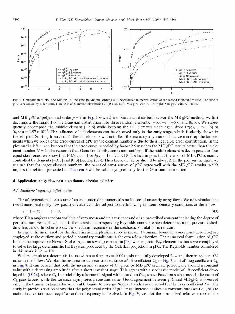
and ME-gPC of polynomial order p = 3 in Fig. 5 when n is of Gaussian distribution. For the ME-gPC method, we firstdecompose the support of the Gaussian distribution into three random elements: (�1,�6], [�6,6] and [6,1). We subse-quently decompose the middle element [�6,6] while keeping the tail elements unchanged since Pr(n 2 (�1,�6] or[6,1)) = 1.97 · 10�9. The influence of tail elements can be observed only in the early stage, which is clearly shown inthe left plot. Starting from t � 0.5, the tail elements will not affect the accuracy any more. Thus, we can drop the tail ele-ments when we re-scale the error curves of gPC by the element number N due to their negligible error contribution. In theplot on the left, it can be seen that the error curve re-scaled by factor 2.5 matches the ME-gPC results better than the ele-ment number N = 4. The reason is that Gaussian distribution is non-uniform. If the middle element is decomposed to fourequidistant ones, we know that Pr(I[�6,3] = 1 or I[3,6] = 1) = 2.7 · 10�3, which implies that the error of ME-gPC is mainlycontrolled by elements [�3,0] and [0,3] (see Eq. (33)). Thus the scale factor should be about 2. In the plot on the right, wecan see that for larger element numbers, the re-scaled error curves of gPC agree well with the ME-gPC results, whichimplies the relation presented in Theorem 5 will be valid asymptotically for the Gaussian distribution.

4. Application: noisy flow past a stationary circular cylinder

4.1. Random-frequency inflow noise

The aforementioned issues are often encountered in numerical simulations of unsteady noisy flows. We now simulate thetwo-dimensional noisy flow past a circular cylinder subject to the following random boundary conditions at the inflow

u ¼ 1þ rY ; v ¼ 0; ð49Þwhere Y is a uniform random variable of zero mean and unit variance and r is a prescribed constant indicating the degree ofperturbation. For each value of Y, there exists a corresponding Reynolds number, which determines a unique vortex shed-ding frequency. In other words, the shedding frequency in the stochastic simulation is random.

In Fig. 6 the mesh used for the discretization in physical space is shown. Neumann boundary conditions (zero flux) areemployed at the outflow and periodic boundary conditions in the cross-flow direction. The numerical formulation of gPCfor the incompressible Navier–Stokes equations was presented in [25], where spectral/hp element methods were employedto solve the large deterministic PDE system produced by the Galerkin projection in gPC. The Reynolds number consideredin this work is Re = 100.

We first simulate a deterministic case with r = 0 up to t = 1000 to obtain a fully developed flow and then introduce 10%noise at the inflow. We plot the instantaneous mean and variance of lift coefficient CL in Fig. 7, and of drag coefficient CD

in Fig. 8. It can be seen that both the mean and variance of CL given by ME-gPC oscillate periodically around a constantvalue with a decreasing amplitude after a short transient stage. This agrees with a stochastic model of lift coefficient deve-loped in [18,26], where CL is modeled by a harmonic signal with a random frequency. Based on such a model, the mean ofCL goes to zero while the variance asymptotes a constant value. Good agreement between gPC and ME-gPC is observedonly in the transient stage, after which gPC begins to diverge. Similar trends are observed for the drag coefficient CD. Thestudy in previous section shows that the polynomial order of gPC must increase at about a constant rate (see Eq. (38)) tomaintain a certain accuracy if a random frequency is involved. In Fig. 9, we plot the normalized relative errors of the

xy

-10 0 10 20

-5

0

5

Fig. 6. Schematic of the domain for noisy flow past a circular cylinder. The size of the domain is [�15D, 25D] · [�9D,9D] and the cylinder is at the originwith diameter D = 1. The mesh consists of 412 triangular elements.

0 50 100 1500

0.02

0.04

0.06

0.08

0.1

0.12

tU/D

Var

ianc

e of

CL

ME-gPC: N=20, p=8gPC: p=8gPC: p=15

0 50 100 150–0.4

–0.3

–0.2

–0.1

0

0.1

0.2

0.3

0.4

tU/D

Mea

n of

CL

ME-gPC: N=20, p=8gPC: p=8gPC: p=15Deterministic

Fig. 7. Evolution of mean (left) and variance (right) of lift coefficient. Y is uniform in ½�ffiffiffi3p

;ffiffiffi3p�. r = 0.1.


variance of the lift coefficient using the results given by ME-gPC with N = 20 and M = 8 as a reference. It can be seen thatthe errors of gPC increase quickly to O(1). ME-gPC with N = 20 and p = 6 reaches an error of O(10�2) at t � 135. We notethat errors less than 10�5 are not shown because the output data are truncated after the fifth digit.

In Section 3 we have shown that the error of ME-gPC at a fixed time can be estimated from that of gPC of the samepolynomial order but shifted by a factor N. Here we cannot use this result directly because the decomposition of randomshedding frequencies is not necessarily uniform although the noise at the inflow is uniform. However, we can estimate thescaling factor from the simulation results for the errors of gPC and ME-gPC of sixth order, which is about 12. Using thisvalue we know that the error of ME-gPC with N = 20 and M = 8 at tU/D = 150 should be roughly equal to the error ofeighth-order gPC at tU/D = 150/12, which is O(10�3). Thus, ME-gPC with N = 20 and M = 8 can provide accurate resultsin the range tU/D 6 150, corresponding to about 20 shedding periods after the transient stage. In contrast, gPC providesaccurate result up to less than two shedding periods.

In Fig. 10 the RMS of vorticity is plotted. The global structure is (approximately) symmetric and the values of RMS ofvorticity are decreasing gradually from the front stagnation point, through the boundary layers, into the wake. This sug-gests that the vorticity behind the cylinder should contain a harmonic signal A(x,Y)cos(2pfv(Y)t) with random frequenciesfv. The RMS of such a harmonic response will approach

RY A2ðx; Y Þf ðY Þ=2dY as t!1, where f(Y) is the PDF of Y. Since

the flux of vorticity decreases in the x direction due to viscous diffusion, the value of A(x,Y) should also decrease in the x

direction. This explains qualitatively why we only observe decreasing RMS values of vorticity in the wake without the vonKarmon vortex street.

4.2. Random-amplitude inflow noise

In this section we consider another noisy boundary condition at the inflow

u ¼ 1þ rn cos 2pfint; v ¼ 0; ð50Þwhere we add a harmonic signal with a random amplitude into the inflow. We use fin = 0.75fs, where fs is the vortex shed-ding frequency at Re = 100. Let n be a uniform random variable with zero mean and unit variance. We set r to 0.1.

0 50 100 1501.36

1.37

1.38

1.39

1.4

1.41

tU/D

Mea

n of

CD

ME-gPC: N=20, p=8gPC: p=8gPC: p=15Deterministic

0 50 100 1500.04

0.05

0.06

0.07

0.08

0.09

0.1

tU/D

Var

ianc

e of

CD

ME-gPC: N=20, p=8gPC: p=8gPC: p=15

Fig. 8. Evolution of mean (left) and variance (right) of drag coefficient. Y is uniform in ½�ffiffiffi3p

;ffiffiffi3p�. r = 0.1.

0 10 20 30 40 50 60 70 80 90 100 110 120 130 140 150

10–4

10–3

10–2

10–1

100

tU/D

Err

or o

f CL

gPC: p=6gPC: p=8gPC: p=15ME-gPC: N=20, p=6

Fig. 9. Evolution of relative errors of instantaneous variance of lift coefficients given by gPC and ME-gPC. The results obtained from ME-gPC withN = 20 and M = 8 are used as a reference.

Fig. 10. Instantaneous spatial distribution of RMS of vorticity at tU/D = 100. N = 20 and M = 8.


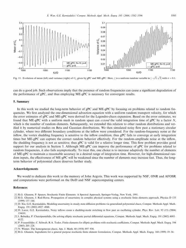
In Fig. 11 we compare the mean and variance of CL given by gPC and ME-gPC of the same order M = 8, where N = 10for the ME-gPC. We see that eighth-order gPC can capture all the statistics up to the second-order in the range oftU/D 6 150 in contrast to the fast divergence of gPC for the random-frequency noise. Numerical experiments show thatfor the boundary condition (50) the frequency of CL is not sensitive to the boundary noise, where the vortex shedding fre-quency at Re = 100 is dominant. Thus, the error of gPC increases much slower than the first case. A similar example isnoisy flow past an oscillating circular cylinder [4], where the frequency is also not sensitive to the noise and thus gPC

1000 1050 1100 1150–0.4

–0.3

–0.2

–0.1

0

0.1

0.2

0.3

0.4

tU/D

Mea

n of

CL

ME-gPC: N=10, p=8gPC: p=8

1000 1050 1100 11500

0.01

0.02

0.03

0.04

0.05

0.06

0.07

0.08

0.09

0.1

tU/D

Var

ianc

e of

CL

ME-gPC: N=10, p=8gPC: p=8

Fig. 11. Evolution of mean (left) and variance (right) of CL given by gPC and ME-gPC. Here, n is a uniform random variable in ½�ffiffiffi3p

;ffiffiffi3p� with r = 0.1.


can do a good job. Such observations imply that the presence of random frequencies can cause a significant degradation ofthe performance of gPC, and thus employing ME-gPC is necessary for convergent results.

5. Summary

In this work we studied the long-term behavior of gPC and ME-gPC by focusing on problems related to random fre-quencies. We first analyzed the one-dimensional advection equation with a uniform random transport velocity, for whichthe error estimates of gPC and ME-gPC were derived for the Legendre-chaos expansion. Based on the error estimates, wefound that ME-gPC with a uniform mesh in random space can extend the valid integration time of gPC by a factor N,which is the number of random elements. Subsequently, we extended this relation to other random distributions and ver-ified it by numerical studies on Beta and Gaussian distributions. We then simulated noisy flow past a stationary circularcylinder, where two different boundary conditions at the inflow were considered. For the random-frequency noise at theinflow, the vortex shedding frequency is sensitive to the inflow condition; thus gPC fails to converge at early integrationtimes but ME-gPC can capture the correct random behavior effectively. For the random-amplitude noise at the inflow,the shedding frequency is not as sensitive; thus gPC is valid for a relative longer time. This flow problem provides goodsupport for our analysis in Section 3. Although ME-gPC can improve the performance of gPC for problems related torandom frequencies, it also fails asymptotically. To treat this, one choice is to increase adaptively the number of elementsof ME-gPC to maintain a reasonable accuracy in a desired range of integration time. However, for high-dimensional ran-dom inputs, the effectiveness of ME-gPC will be weakened since the number of elements may increase fast. Thus, the long-term behavior of polynomial chaos deserves further study.

Acknowledgements

We would to dedicate this work to the memory of John Argyris. This work was supported by NSF, ONR and AFOSRand computations were performed on the DoD and NSF supercomputing centers.

References

[1] R.G. Ghanem, P. Spanos, Stochastic Finite Elements: A Spectral Approach, Springer-Verlag, New York, 1991.[2] R.G. Ghanem, J. Red-Horse, Propagation of uncertainty in complex physical systems using a stochastic finite elements approach, Physica D 133

(1999) 137–144.[3] D. Xiu, G.E. Karniadakis, Modeling uncertainty in steady state diffusion problems via generalized polynomial chaos, Comput. Methods Appl. Math.

Engrg. 191 (2002) 4927–4948.[4] D. Lucor, G.E. Karniadakis, Noisy inflows cause a shedding-mode switching in flow past an oscillating cylinder, Phys. Rev. Lett. 92 (15) (2004)

154101.[5] I. Babuska, P. Chatzipantelidis, On solving elliptic stochastic partial differential equations, Comput. Methods Appl. Mech. Engrg. 191 (2002) 4093–

4122.[6] P. Frauenfelder, C. Schwab, R.A. Todor, Finite elements for elliptic problems with stochastic coefficients, Comput. Methods Appl. Mech. Engrg. 194

(2005) 205–228.[7] N. Wiener, The homogeneous chaos, Am. J. Math. 60 (1938) 897–936.[8] R.G. Ghanem, Ingredients for a general purpose stochastic finite element formulation, Comput. Methods Appl. Mech. Engrg. 168 (1999) 19–34.


[9] R.G. Ghanem, Stochastic finite elements for heterogeneous media with multiple random non-Gaussian properties, ASCE J. Engrg. Mech. 125 (1)(1999) 26–40.

[10] D. Xiu, G.E. Karniadakis, The Wiener–Askey polynomial chaos for stochastic differential equations, SIAM J. Sci. Comput. 24 (2) (2002) 619–644.[11] O.P.L. Maitre, H.N. Njam, R.G. Ghanem, O.M. Knio, Uncertainty propagation using Wiener–Haar expansions, J. Comput. Phys. 197 (2004) 28–57.[12] O.P.L. Maitre, H.N. Njam, R.G. Ghanem, O.M. Knio, Multi-resolution analysis of Wiener-type uncertainty propagation schemes, J. Comput. Phys.

197 (2004) 502–531.[13] M.K. Deb, I. Babuska, J.T. Oden, Solution of stochastic partial differential equations using Galerkin finite element techniques, Comput. Methods

Appl. Mech. Engrg. 190 (2001) 6359–6372.[14] I. Babuska, R. Tempone, G.E. Zouraris, Galerkin finite element approximations of stochastic elliptic differential equations, SIAM J. Numer. Anal. 42

(2) (2004) 800–825.[15] G.E. Karniadakis, S.J. Sherwin, Spectral/hp Element Methods for CFD, second ed., Oxford University Press, 2005.[16] C. Schwab, p- and hp-Finite Element Methods: Theory and Applications in Solid and Fluid Mechanics, Clarendon Press, Oxford, 1998.[17] S.A. Orszag, L.R. Bissonnette, Dynamical properties of truncated Wiener–Hermite expansions, Phys. Fluids 10 (12) (1967) 2603–2613.[18] D. Lucor, Generalized Polynomial Chaos: Applications to Random Oscillators and Flow-structure Interactions, Ph.D. thesis, Brown University,

Division of Applied Mathematics, 2004.[19] X. Wan, G.E. Karniadakis, An adaptive multi-element generalized polynomial chaos method for stochastic differential equations, J. Comput. Phys.

209 (2) (2005) 617–642.[20] X. Wan, G.E. Karniadakis, Multi-element generalized polynomial chaos for arbitrary probability measures, SIAM J. Sci. Comput., in press.[21] W. Gautschi, On generating orthogonal polynomials, SIAM J. Sci. Stat. Comput. 3 (3) (1982) 289–317.[22] D. Gottlieb, S.A. Orszag, Numerical Analysis of Spectral Methods: Theory and Applications, SIAM, Philadelphia, PA, 1977.[23] M. Abramowitz, I.A. Stegun, Handbook of Mathematical Functions, Dover, New York, 1970.[24] M. Ainsworth, Dispersive and dissipative behaviour of high order discontinuous Galerkin finite element method, J. Comupt. Phys. 198 (2004) 106–

130.[25] D. Xiu, G.E. Karniadakis, Modeling uncertainty in flow simulations via generalized polynomial chaos, J. Comput. Phys. 187 (2003) 137–167.[26] X. Wan, Multi-element Generalized Polynomial Chaos for Differential Equations with Random Inputs: Algorithms and Applications, Ph.D. thesis,

Brown University, Division of Applied Mathematics (in preparation).

Long-term behavior of polynomial chaos in stochastic ﬂow ...

Documents

Transcript of Long-term behavior of polynomial chaos in stochastic ﬂow ...