Logical Functions and

Operators Chapter 8

Objectives

After studying this chapter you

should be able to: • Understand how MATLAB interprets

relational and logical operators

• Use the find function

• Understand the appropriate uses of the if/else

family of commands

• Understand the switch/case structure

We can consider algorithms to be practical solutions

to problems. These solutions are not answers, but

specific instructions for getting answers.

Introduction - Algorithms

• Before writing a program:

• Have a thorough understanding of the problem

• Carefully plan an approach for solving it

• While writing a program:

• Know what “building blocks” are available

• Use good programming principles

4

Introduction - Algorithms

• Computing problems

• All can be solved by executing a series of

actions in a specific order

• Algorithm: procedure in terms of

• Actions to be executed

• The order in which these actions are to be

executed

• Program control

• Specify order in which statements are to be

executed

5

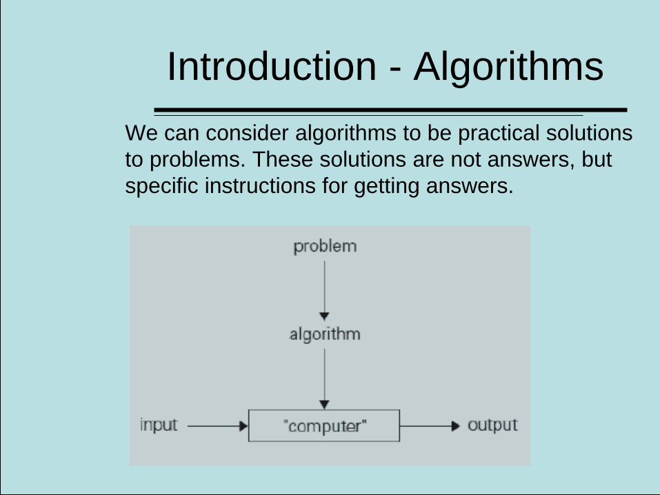
Algorithms

Pseudocode and Flowcharts

• Description of the algorithm in a standard form

(easy to understand for anyone)

• Language independent

The constructs used to build algorithms can be

described in two ways:

• Pseudocode (mix. of English and

programming language)

• Flowcharts (using charts)

Algorithms –

Pseudocode/Flowcharts

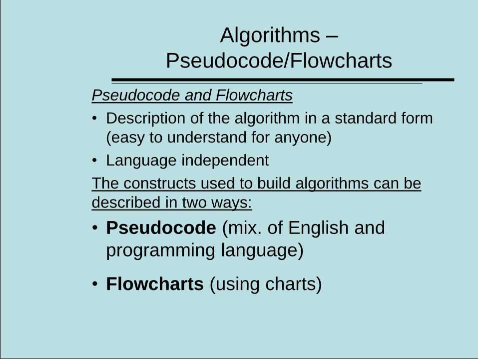
Pseudocode

• Artificial, informal language that helps us

develop algorithms

• Similar to everyday English

• Not actually executed on computers

• Helps us “think out” a program before writing it

• Easy to convert into a corresponding

program

• Consists only of executable statements

7

Algorithm – Pseudocode/Flowchart

Pseudocode

if criterion 1

action 1

else if criterion 2

action 2

else if criterion 3

action 3

otherwise

action 4

Choice and decision-making – Pseudocode Example

if (criterion 1)

action_1;

else if (criterion 2)

action_2;

else if (criterion 3)

action_3;

else

action_4;

Pseudo-code Example

• You’ve been asked to create a

program to convert miles/hr to ft/s.

The output should be a table,

complete with title and column

headings

Outline the steps

• Define a vector of mph values

• Convert mph to ft/s

• Combine the mph and ft/s vectors

into a matrix

• Create a table title

• Create column headings

• Display the table

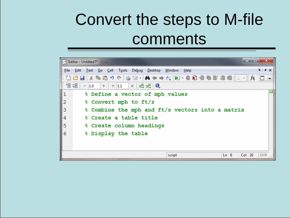
Convert the steps to M-file

comments

Insert the MATLAB code

between the comments

Flowchart

• Graphical representation of an algorithm

• Drawn using certain special-purpose symbols

connected by arrows called flowlines

Single-entry/single-exit control structures

• Connect exit point of one control structure to

entry point of the next (control-structure

stacking)

• Makes programs easy to build

13

Control Structures

Flowcharts

• Graphical representation of an algorithm

• Drawn using certain special-purpose symbols connected by arrows called flowlines

Start/ Stop

Acomputational result assigned to a var. at LHS

input / ouput operation

A point where a choice is made by two alternatives

Direction of program flow bw steps

İterative or counting loop

Flowcharts - Example

Temperature conversion from F to Celcius

Start

Tell user to enter

temp. in F

Get temp.

in F (temp_F)

Calculate temp.

(temp_C) temp_C=5/9*(temp_F- 32)

Print temp.

in C (temp_C)

Stop

Flow Charting

• Especially appropriate for more

complicated programs

• Create a big picture graphically

• Convert to pseudo-code

Start

Define a vector

of miles/hour

Calculate the

ft/sec vector

Combine into a

table

Create an output

table using disp

and fprintf

End

This flowchart

represents the

mph to ft/s

problem

• At the final step, the algorithm,

expressed in either flowcharts or

pseudocodes, are translated into

the programming language

(MATLAB, C, Fortran, etc.)

Coding an algorithm:

Programming

Programming Style

1. Comments section

a. The name of the program and any key words in

the first line.

b. The date created, and the creators' names in

the second line.

c. The definitions of the variable names for every

input and output variable. Include definitions of

variables used in the calculations and units of

measurement for all input and all output variables!

d. The name of every user-defined function called

by the program.

1-27

2. Input section Include input data

and/or the input functions and

comments for documentation.

3. Calculation section

4. Output section This section might

contain functions for displaying the

output on the screen.

1-28

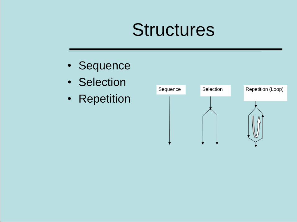
Structures

• Sequence

• Selection

• Repetition Sequence Selection Repetition (Loop)

8.1 Relational and Logical Operators

• Sequence and Repetition

structures require comparisons to

work

• Relational operators make those

comparisons

• Logical operators allow us to

combine the comparisons

Complex. a + b i

• a and b are real numbers

• i is an imaginary number. ( i2= -1 )

Different types of Variables

Integer.

positive whole numbers {1, 2, 3,... }

negative whole numbers {-1, -2, -3,... }

zero {0}

Matlab Notation

N= a+bi

or

N=a+bj

Real. real number.

Matrix index (ex: B(2,1) )

Counters

All calculus results…

Complex calculus

Geometry Vector calculus

A= 5+10i;

B=2.5+20.2j;

Examples:

Numerical Variables

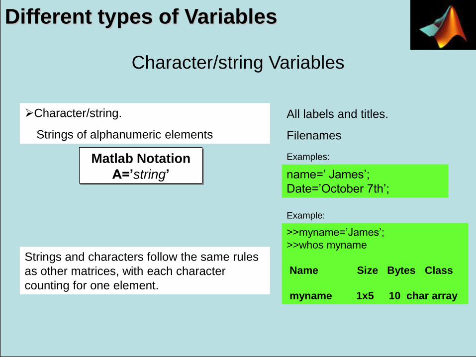
Character/string.

Strings of alphanumeric elements

Different types of Variables

Matlab Notation

A=’string’

All labels and titles.

Filenames

Strings and characters follow the same rules

as other matrices, with each character

counting for one element.

>>myname=’James’;

>>whos myname

Name Size Bytes Class

myname 1x5 10 char array

Example:

name=’ James’;

Date=’October 7th’;

Examples:

Character/string Variables

Logical Variables

Logical Variables or Boolean.

Logical expression with 2 states:

0 or 1

which means: false or true

Condition statements

Decision making

>>A=true

A = 1

>> whos A

Name Size Bytes Class

A 1x1 1 logical array

Example:

>>B=false

B = 0

>> whos B

Name Size Bytes Class

B 1x1 1 logical array

Example:

Different types of Variables

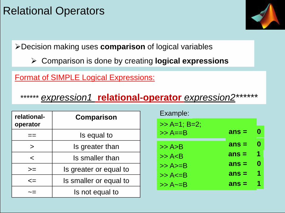
Relational Operators

Decision making uses comparison of logical variables

Comparison is done by creating logical expressions

Format of SIMPLE Logical Expressions:

****** expression1 relational-operator expression2******

relational-

operator Comparison

== Is equal to

> Is greater than

< Is smaller than

>= Is greater or equal to

<= Is smaller or equal to

~= Is not equal to

>> A=1; B=2;

>> A==B

Example:

ans = 0

>> A>B ans = 0

>> A<B ans = 1

>> A>=B ans = 0

>> A<=B ans = 1

>> A~=B ans = 1

Comparisons are either true

or false

• Most computer programs use the

number 1 for true and 0 for false

The results of a comparison are used in

selection structures and repetition

structures to make choices

MATLAB compares corresponding

elements and determines if the

result is true or false for each

In order for MATLAB to decide a

comparison is true for an entire

matrix, it must be true for every

element in the matrix

For example, suppose that x = [6,3,9] and

y = [14,2,9].

The following MATLAB session shows some

examples.

>>z = (x < y)

z =

1 0 0

>>z = (x ~= y)

z =

1 1 0

>>z = (x > 8)

z =

0 0 1

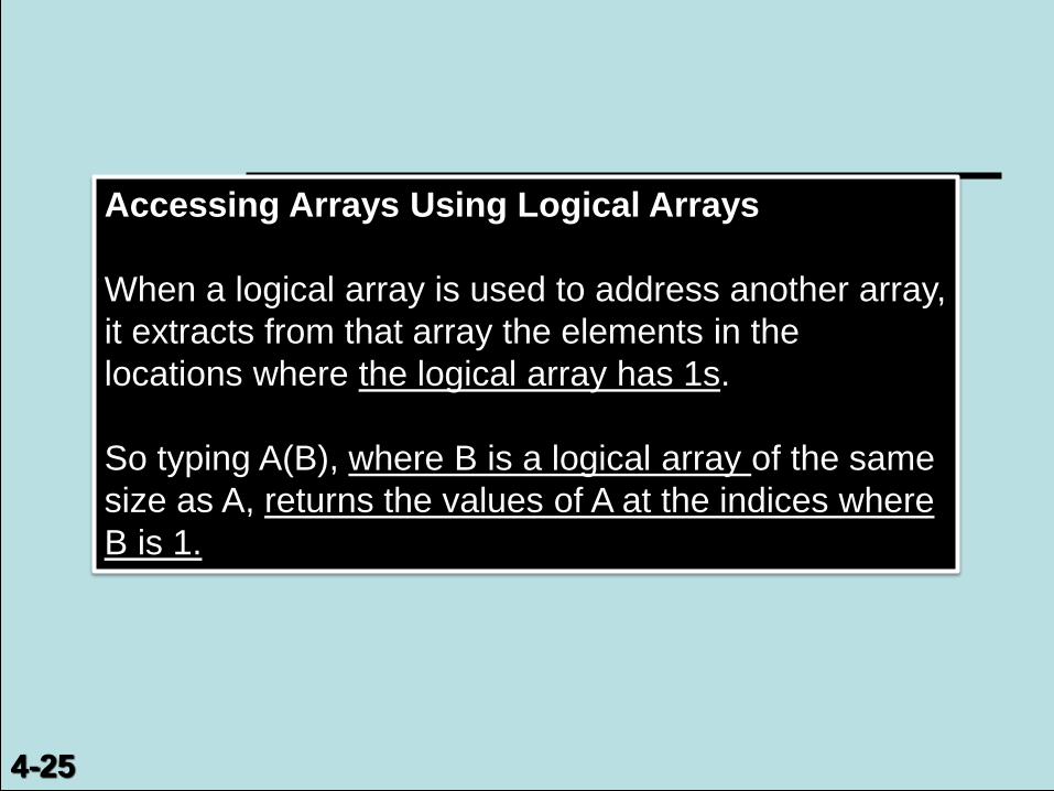
Accessing Arrays Using Logical Arrays

When a logical array is used to address another array,

it extracts from that array the elements in the

locations where the logical array has 1s.

So typing A(B), where B is a logical array of the same

size as A, returns the values of A at the indices where

B is 1.

4-25

The relational operators can be used for array addressing.

For example, with x = [6,3,9] and y = [14,2,9], typing

z = x(x<y)

finds all the elements in x that are less than the

corresponding elements in y.

The result is z = 6.

4-21

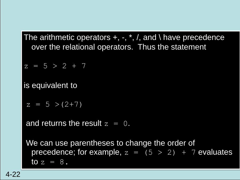
The arithmetic operators +, -, *, /, and \ have precedence

over the relational operators. Thus the statement

z = 5 > 2 + 7

is equivalent to

z = 5 >(2+7)

and returns the result z = 0.

We can use parentheses to change the order of precedence; for example, z = (5 > 2) + 7 evaluates

to z = 8.

4-22

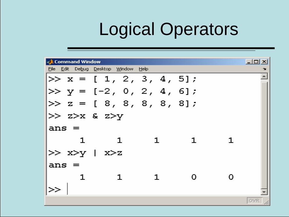
Logical Operators

Format of COMPOUND Logical Expressions:

(exp1 relational-op exp2) Logical operator (exp3 relational-op exp4)

Logical

operator operation

& and

| or

xor or (exclusive)

~ not

A B C= A&B

0 0 0

0 1 0

1 0 0

1 1 1

A B C= A|B

0 0 0

0 1 1

1 0 1

1 1 1

A B C= xor(A,B)

0 0 0

0 1 1

1 0 1

1 1 0

Truth

Table ~(A&B)

1

1

1

0

~xor(A,B)

1

0

0

1

~(A|B)

1

0

0

0

Logical Variables

>> A=1; B=2;

>> (A==B) & (A>B)

Examples:

>> (A<B) & (A==B) ans = 0

ans = 0

>> (A==B) | (A>B) ans = 0

>> (A<B) | (A==B) ans = 1

>> xor( (A==B), (A<B) ) ans = 1

>> ~(A<B) ans = 0

>> xor( (A~=B), (A<B) )

>> ~(A>B) ans = 1

ans = 0

>> (A>0) & (B>A) ans = 1

>> (A>0) & (B>A)&(B<0) ans = 0

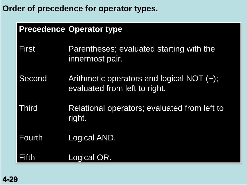
Precedence Operator type

First Parentheses; evaluated starting with the

innermost pair.

Second Arithmetic operators and logical NOT (~);

evaluated from left to right.

Third Relational operators; evaluated from left to

right.

Fourth Logical AND.

Fifth Logical OR.

4-29

Order of precedence for operator types.

Logical Operators

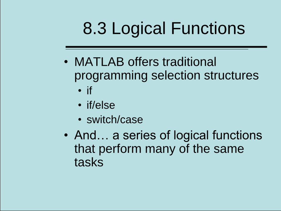
8.3 Logical Functions

• MATLAB offers traditional programming selection structures

• if

• if/else

• switch/case

• And… a series of logical functions that perform many of the same tasks

find

• The find command searches a

matrix and identifies which

elements in that matrix meet a

given criteria.

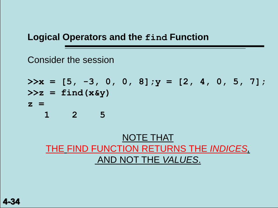
Logical Operators and the find Function

Consider the session

>>x = [5, -3, 0, 0, 8];y = [2, 4, 0, 5, 7];

>>z = find(x&y)

z =

1 2 5

NOTE THAT

THE FIND FUNCTION RETURNS THE INDICES,

AND NOT THE VALUES.

4-34

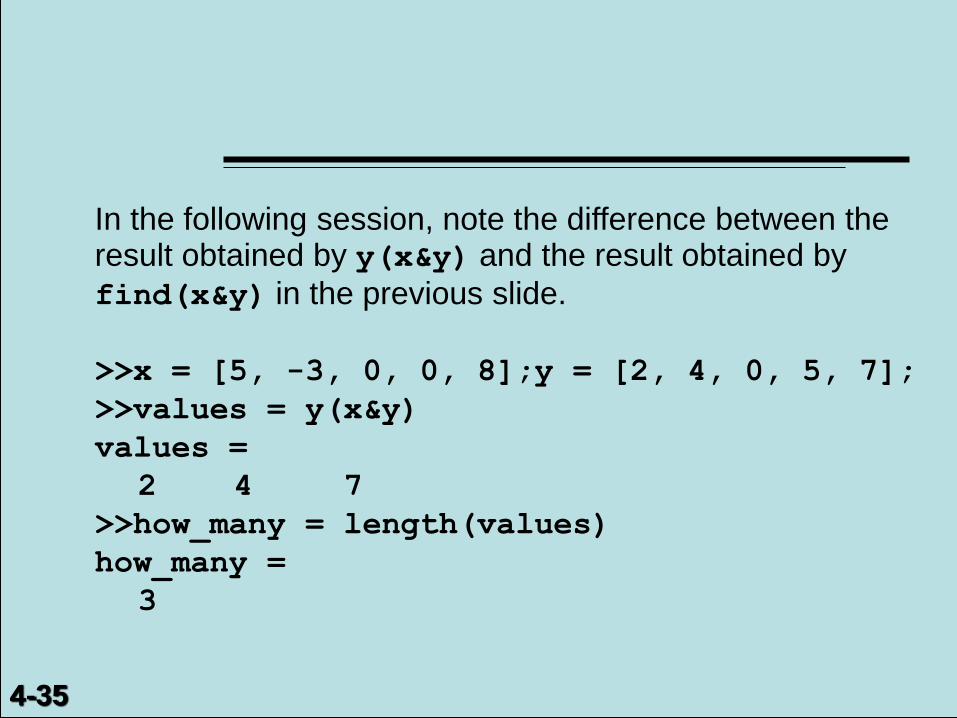
In the following session, note the difference between the result obtained by y(x&y) and the result obtained by

find(x&y) in the previous slide.

>>x = [5, -3, 0, 0, 8];y = [2, 4, 0, 5, 7];

>>values = y(x&y)

values =

2 4 7

>>how_many = length(values)

how_many =

3

4-35

For example…

• The US Naval Academy requires

applicants to be at least 5’6” tall

• Consider this list of applicant heights

• 63”, 67”, 65”, 72”, 69”, 78”, 75”

• Which applicants meet the criteria?

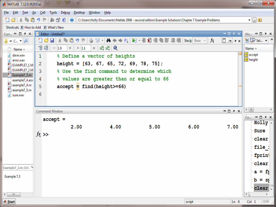
The find function returns the index number

for elements that meet a criteria

index numbers

element values

index numbers

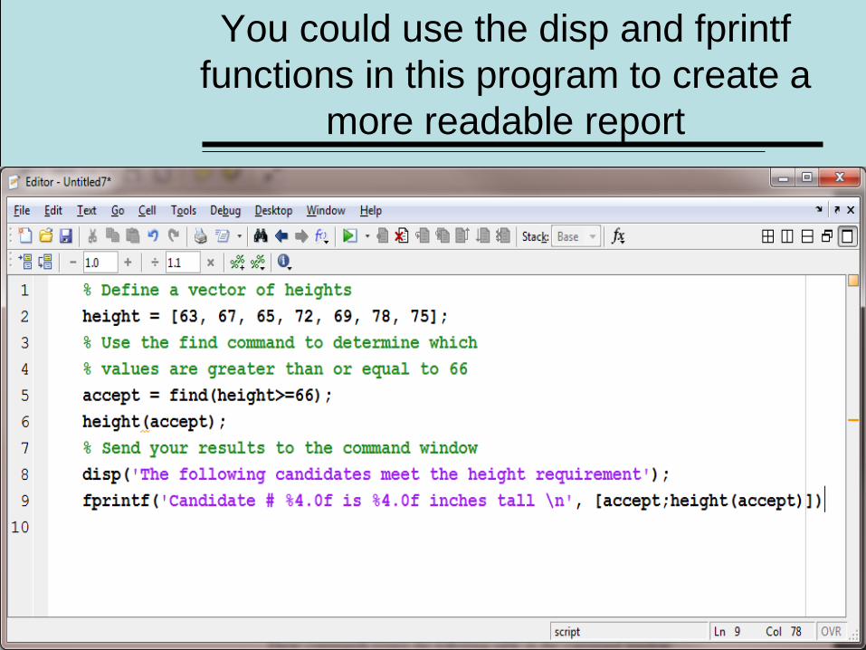
You could use the disp and fprintf

functions in this program to create a

more readable report

You could also make a table of those who

do not meet the height requirement

By combining relational and logical operators

you can create fairly complicated search

criteria

• Assume applicants must be at least 18

years old and less than 35 years old

• They must also meet the height

requirement

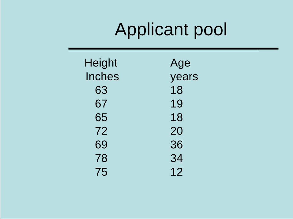
Applicant pool

Height Age

Inches years

63 18

67 19

65 18

72 20

69 36

78 34

75 12

Let’s use Pseudo-code to

plan this program

• Create a 7x2 matrix of applicant

height and age information

• Use the find command to

determine which applicants are

eligible

• Use fprintf to create a table of

results

This is the M-file program to determine who is eligible

Because we didn’t suppress all the

output, the intermediate calculations

were sent to the command window

The find command can

return either…

• A single index number identifying an

element in a matrix

• A matrix of the row numbers and the

column numbers identifying an

element in a matrix

• You need to specify two results if you want

the row and column designation

• [row, col] = find( criteria)

Imagine you have a matrix of

patient temperature values

measured in a clinic

Station 1 Station 2 Station 3

95.3 100.2 98.6

97.4 99.2 98.9

100.1 99.3 97

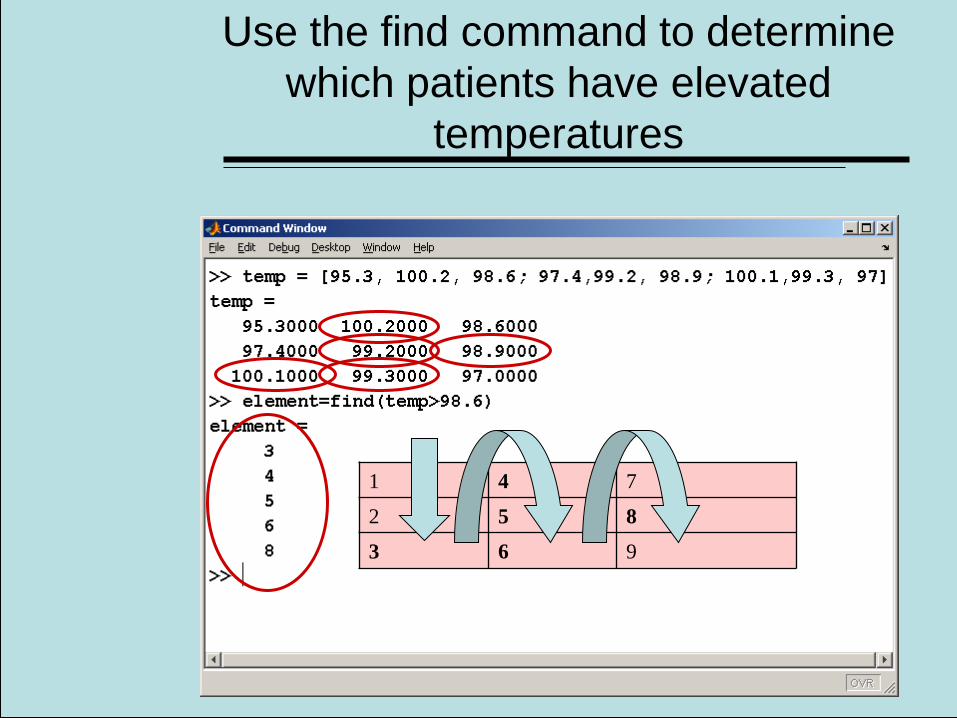
Use the find command to determine

which patients have elevated

temperatures

These elements refer to the single

index number identification scheme

1 4 7

2 5 8

3 6 9

If we want the row and

column…

1,1 1,2 1,3

2,1 2,2 2,3

3,1 3,2 3,3

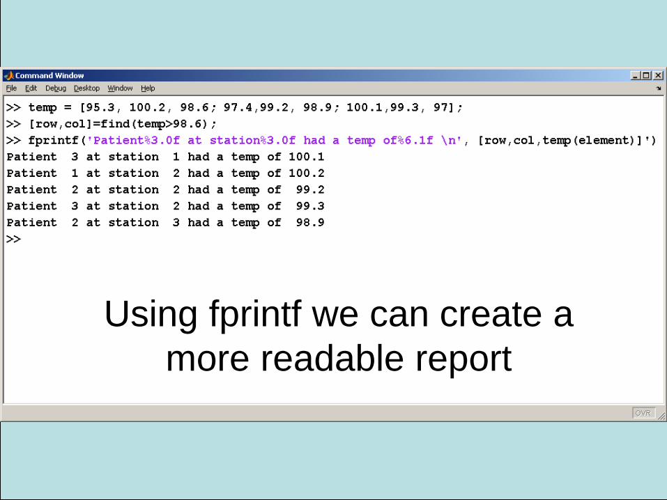
Using fprintf we can create a

more readable report

Flow charting and Pseudo-

code for find Commands Start

Define a vector of x

values

Find the index numbers in the x

matrix for values greater than 9

Use the index numbers to

find the x values

Create an output

table using disp

and fprintf

End

%Define a vector of x values

x=[1,2,3; 10, 5,1; 12,3,2;8, 3,1]

%Find the index numbers of the values in %x

>9

element = find(x>9)

%Use the index numbers to find the x

%values greater than 9 by plugging them

%into x

values = x(element)

% Create an output table

disp('Elements greater than 9')

disp('Element # Value')

fprintf('%8.0f %3.0f \n', [element';values'])