Local entropy averages and projections of fractal...
59
Annals of Mathematics 175 (2012), 1001–1059 http://dx.doi.org/10.4007/annals.2012.175.3.1 Local entropy averages and projections of fractal measures By Michael Hochman and Pablo Shmerkin Abstract We show that for families of measures on Euclidean space which sat- isfy an ergodic-theoretic form of “self-similarity” under the operation of re-scaling, the dimension of linear images of the measure behaves in a semi-continuous way. We apply this to prove the following conjecture of Furstenberg: if X, Y ⊆ [0, 1] are closed and invariant, respectively, under ×m mod 1 and ×n mod 1, where m, n are not powers of the same integer, then, for any t 6= 0, dim(X + tY ) = min{1, dim X + dim Y }. A similar result holds for invariant measures and gives a simple proof of the Rudolph-Johnson theorem. Our methods also apply to many other classes of conformal fractals and measures. As another application, we extend and unify results of Peres, Shmerkin and Nazarov, and of Moreira, concerning projections of products of self-similar measures and Gibbs measures on reg- ular Cantor sets. We show that under natural irreducibility assumptions on the maps in the IFS, the image measure has the maximal possible di- mension under any linear projection other than the coordinate projections. We also present applications to Bernoulli convolutions and to the images of fractal measures under differentiable maps. 1. Introduction 1.1. Background and history. Let dim denote the Hausdorff dimension of a set and let Π d,k denote the space of orthogonal projections from R d to k-dimensional subspaces, with the natural measure. Then it is a classical fact, due in various versions to Marstrand, Mattila and others, that for any Borel set X ⊆ R d , almost every π ∈ Π d,k satisfies (1.1) dim(πX ) = min(k, dim X ). This research was partially supported by the NSF under agreement No. DMS-0635607. M.H. supported by NSF grant 0901534. P.S. acknowledges support from EPSRC grant EP/E050441/1 and the University of Manchester. 1001
Transcript of Local entropy averages and projections of fractal...
Annals of Mathematics 175 (2012), 1001–1059http://dx.doi.org/10.4007/annals.2012.175.3.1
Local entropy averages andprojections of fractal measures
By Michael Hochman and Pablo Shmerkin
Abstract
We show that for families of measures on Euclidean space which sat-
isfy an ergodic-theoretic form of “self-similarity” under the operation of
re-scaling, the dimension of linear images of the measure behaves in a
semi-continuous way. We apply this to prove the following conjecture of
Furstenberg: if X,Y ⊆ [0, 1] are closed and invariant, respectively, under
×m mod 1 and ×n mod 1, where m,n are not powers of the same integer,
then, for any t 6= 0,
dim(X + tY ) = min1, dimX + dimY .
A similar result holds for invariant measures and gives a simple proof of the
Rudolph-Johnson theorem. Our methods also apply to many other classes
of conformal fractals and measures. As another application, we extend and
unify results of Peres, Shmerkin and Nazarov, and of Moreira, concerning
projections of products of self-similar measures and Gibbs measures on reg-
ular Cantor sets. We show that under natural irreducibility assumptions
on the maps in the IFS, the image measure has the maximal possible di-
mension under any linear projection other than the coordinate projections.
We also present applications to Bernoulli convolutions and to the images
of fractal measures under differentiable maps.
1. Introduction
1.1. Background and history. Let dim denote the Hausdorff dimension
of a set and let Πd,k denote the space of orthogonal projections from Rd to
k-dimensional subspaces, with the natural measure. Then it is a classical fact,
due in various versions to Marstrand, Mattila and others, that for any Borel
set X ⊆ Rd, almost every π ∈ Πd,k satisfies
(1.1) dim(πX) = min(k, dimX).
This research was partially supported by the NSF under agreement No. DMS-0635607.
M.H. supported by NSF grant 0901534. P.S. acknowledges support from EPSRC grant
EP/E050441/1 and the University of Manchester.
1001

1002 MICHAEL HOCHMAN and PABLO SHMERKIN
Indeed, the right-hand side is a trivial upper bound: Lipschitz maps cannot
increase dimension, so dimπX ≤ dimX, and πX is a subset of a k-dimensional
subspace, hence dimπX ≤ k. Since this equality holds almost everywhere, we
shall use the term exceptional for projections for which equality fails and call
the right-hand side the expected dimension.
While (1.1) tells us what happens for a typical projection, it is far more
difficult to analyze the image of even the simplest fractals under individual
projections. See Kenyon [21] for a particularly simple and frustrating example.
There are, however, a number of well-known conjectures to the effect that,
for certain sets of combinatorial, arithmetic or dynamical origin, phenomena
which hold typically in the general setting should, for these special sets, always
hold, except in the presence of some evident obstruction. The present work was
motivated by a conjecture of this kind concerning projections of product sets
whose marginals are invariant under arithmetically “independent” dynamics.
Denote the m-fold map of the unit interval by Tm : x 7→ mx mod 1 and
let πx, πy ∈ Π2,1 denote the coordinate projections onto the axes.
Conjecture 1.1 (Furstenberg). Let X,Y ⊆ [0, 1] be closed sets which
are invariant under T2 and T3, respectively. Then
dimπ(X × Y ) = min1,dim(X × Y )
for any π ∈ Π2,1 \ πx, πy.
In the situation above it is evident that πx, πy are exceptions, since they
map X×Y to X or Y , respectively, and a drop in dimension is to be expected.
Note that this conjecture can also be formulated as a result on sumsets.1
For X,Y as above and all s 6= 0,
dim(X + sY ) = min1,dimX + dimY .
Here A+B = a+ b : a ∈ A , b ∈ B.Conjecture 1.1 originates in the late 1960’s. Although it has apparently
not appeared in print, it is related to another conjecture of Furstenberg’s from
around the same time, which appears in [12].
Conjecture 1.2 (Furstenberg, [12]). Let X,Y ⊆ [0, 1] be closed sets
which are invariant under T2 and T3, respectively. Then for any s, t, t 6= 0,
dimX ∩ (s+ tY ) ≤ maxdimX + dimY − 1, 0.
1In the sumset formulation we relied on the identity
dim(X × Y ) = dim(X) + dim(Y ).
This holds in the present case because X has coinciding Hausdorff and box dimension (see,
e.g., [13, Th. 5.1]); in general one only has the inequality dim(X × Y ) ≥ dim(X) + dim(Y ).

LOCAL ENTROPY AVERAGES 1003
The relation between these conjecture is as follows. The sets X ∩ (s+ tY )
are, up to affine coordinate change, the intersections of X × Y with the fibers
of the projections π ∈ Π2,1 \ πx, πy. Heuristically, one expects the following
relation between the dimension of the image and the fibers:
(1.2) dimX × Y = dimπ(X × Y ) + supzdim((X × Y ) ∩ π−1(z)).
This is, for example, the way affine subspaces in Rd behave under linear maps,
as do generic sub-manifolds. If it were true, then Conjectures 1.1 and 1.2 would
be equivalent. If the image under a projection has the expected dimension, then
the fibers would behave as expected as well.
Equation (1.2) is a very strong statement, and simple examples show that
it is not generally true. For quite general sets A ⊆ Rd, it is known that,
under a natural distribution on the k-dimensional subspaces which intersect
A, almost every such subspace intersects A in the expected dimension, i.e., the
larger of dimA− k and 0; see [24, Th. 10.11]. For certain special sets A ⊆ R2,
related in some ways to the product sets we are discussing, a stronger result
was obtained by Furstenberg [13]. For every t 6= 0, there are many (in the
sense of dimension) values of s such that A intersects the line x− ty = s in at
least the expected dimension. However, the uniform upper bounds needed for
Conjecture 1.2 still seems out of reach of current methods.
We refer the reader to [12] for a more detailed discussion of Conjecture 1.2
and some related questions.
1.2. Iterated Function Systems. A related circle of questions concerns pro-
jections of product sets whose marginals are attractors of iterated function sys-
tems (IFSs) on the line. Here again it is believed that, in the absence of some
evident “resonance” between the IFSs, projections should behave as expected.
There was little progress on Conjecture 1.1 until fairly recently. The first
result of this kind is a theorem by C. G. Moreira [25]2 for pairs of regular IFSs,
i.e., systems of C1+ε contractions on the line satisfying the strong separation
condition (see §11). Moreira assumes that at least one of the IFSs is strictly
nonlinear, i.e., cannot be conjugated to a linear one, and that a certain irra-
tionality condition is satisfied between the IFSs. Under these hypotheses he
shows that if X,Y are the attractors, then the sumset X + Y , which is the
projection of X × Y under π(x, y) = x+ y, has the expected dimension.
More recently Y. Peres and P. Shmerkin [31] solved the problem for pro-
jections of X × Y when X,Y are attractors of linear IFSs satisfying an irra-
tionality condition (namely, that the logarithms of some pair of contraction
ratios is rationally independent). This class of examples includes some special
2The proof in [25] is incomplete; see, e.g., [31].

1004 MICHAEL HOCHMAN and PABLO SHMERKIN
cases of Conjecture 1.1. For example, the standard middle-third Cantor set is
both T3-invariant and the attractor of an IFS with contraction ratio 1/3. With
an eye to Furstenberg’s conjecture, these methods can be pushed to apply to
Tm-invariant subsets of [0, 1] that are shifts of finite type with respect to the
base-m coding. See also [10] for an extension to some nonconformal attractors
on the plane.
With regard to the question of projecting measures rather than sets,
Nazarov, Peres and Shmerkin [29] recently established some results for pro-
jections of Hausdorff measure on X × Y , where X,Y are now attractors of
linear IFSs in which, additionally, all contracting maps have the same contrac-
tion ratio. (While these assumptions are quite special, in this case they also
establish a stronger result using correlation dimension rather than Hausdorff
dimension.)
It is interesting to note that the methods of Moreira and of Peres-Shmerkin
are quite different and rely heavily on their respective assumptions, i.e., strict
nonlinearity and linearity of the IFSs. This leaves open the case of a pair of
IFSs which are both nonlinearly conjugated to linear IFSs. Their methods also
do not give any information about behavior of measures on regular IFSs.
Finally, similar questions may be asked about multidimensional attractors
of IFSs rather than products one-dimensional ones. For the case of 2-dimen-
sional linear IFSs, Peres and Shmerkin [31] showed that, assuming that the
orthogonal part of the contractions include at least one irrational rotation, all
projections behave as expected. Unfortunately these methods do not work for
dimension d ≥ 3 and again give no information about measures.
1.3. Results. In this work we develop a method for bounding from be-
low the dimension of projections of measures which exhibit certain statistical
self-similarity. Before describing the general result, we summarize our main
applications.
The first is a resolution of Conjecture 1.1 in its full generality. In fact,
we establish a stronger statement concerning invariant measures. Recall that
for a probability measure µ on a metric space, the lower Hausdorff dimension
dim∗ µ is defined as
dim∗ µ = infdim(A) : µ(A) > 0.
Also, write dimµ = α to indicate that
limr↓0
µ(Br(x))
log r= α for µ-a.e. x.
In this case α is the exact dimension of µ and dim∗ µ = dimµ, but note that
dimµ is not always defined. See Section 3 for a discussion of dimension.

LOCAL ENTROPY AVERAGES 1005
Theorem 1.3. Let µ, ν be Borel probability measures on [0, 1] which are
invariant under Tm, Tn, respectively, and m,n are not powers of the same
integer. Then for every π ∈ Π2,1 \ πx, πy,
dim∗ π(µ× ν) = min1, dim∗(µ× ν).
If µ, ν are exact dimensional, then the above holds for dim instead of dim∗.
Note that both the conjecture above and the theorem hold trivially in
dimension zero. From the theorem one proves the conjecture using the varia-
tional principle to relate the dimension of sets and measures; see Section 10.4.
Theorem 1.3 also leads to a very short proof of the Rudolph-Johnson
theorem (see §10.5): If m,n are not powers of the same integer, µ is a proba-
bility measure on [0, 1] invariant under both Tm and Tn, and all ergodic com-
ponents have positive entropy for one (equivalently both) of the maps, then
µ =Lebesgue measure. Unfortunately, neither this proof nor our methods pro-
vide a hint about how to approach the long-standing conjecture about the
entropy zero case.
For the next result, we require some notation. For general definitions
regarding IFSs, see Sections 9 and 11. Given a contracting smooth map f on
[0, 1], we let
(1.3) λ(f) = − log(f ′(x)),where x is the fixed point of f.
Furthermore, if I = fi : i ∈ Λ is a regular IFS (see §11 for the definition),
we let
L(I) = λ(fx1 · · · fxn) : n ∈ N, x1, . . . , xn ∈ Λ.
Theorem 1.4. Let I(i) = f (i)j : j ∈ Λi, i = 1, . . . , d be regular IFSs
with attractor Xi. Suppose the following holds.
Minimality assumption. The set L(I(1))×· · ·×L(I(d)) is dense in the
quotient space (Rd,+)/∆, where ∆ is the diagonal subgroup of Rd.Then for any globally supported Gibbs measures µi on Xi corresponding
to arbitrary Holder potentials, and for any projection π(x) =∑i tixi with all
ti nonzero,
dim (π(µ1 × · · · × µd)) = min(1, dim(µ1) + · · ·+ dim(µd)).
A classical result of R. Bowen shows that Hausdorff measure on a regular
Cantor set is equivalent to a Gibbs measure for an appropriate potential. We
therefore have
Corollary 1.5. If Xi are attractors of IFSs satisfying the hypotheses of
the theorem, then for any π ∈ Πd,k,
(1.4) dimπ(X1 × · · · ×Xd) = min1,dimX1 + · · ·+ dimXd.

1006 MICHAEL HOCHMAN and PABLO SHMERKIN
The minimality condition in Theorem 1.4 is satisfied, for example, when
there are d rationally independent numbers among the numbers λ(f(i)j ). Thus
Theorem 1.4 (and its corollary) generalizes and extends the aforementioned
results of Moreira [25], Peres-Shmerkin [31] and Nazarov-Peres-Shmerkin [29].
We note that Theorem 1.4 does not make any assumptions about the linear
or nonlinear nature of the IFSs, and neither does the proof, which provides
a unified treatment of the known cases. We also remark that Moreira [pri-
vate communication] has shown that, for d = 2, the minimality assumption
holds automatically when one of the IFS is not conjugated to a linear IFS. In
the linear case, however, the minimality assumption may fail to hold and is
necessary; see [31] for a discussion.
For self-similar sets and measures in Rd (see §9), we have
Theorem 1.6. Let fi : i ∈ Λ be an iterated function system on Rdwith the strong separation condition consisting of similarities, and let µ be a
self-similar measure on its attractor. Let Oi denote the orthogonal part of the
similarity fi, and suppose that
Minimality assumption. The action (by right composition) of the
semigroup generated by Oi on Πd,k is topologically minimal ; i.e., for some
(equivalently any) π ∈ Πd,k, the orbit
πOi1 · · ·Oik : i1, . . . , ik ∈ Λ
is dense in Πd,k.
Then for every C1 map g : suppµ → Rk without singular points, gµ is
exact dimensional and
dim(gµ) = min(k, dimµ).
It is well known that, under the strong separation condition, for a self-
similar set of dimension α, the α-dimensional Hausdorff measure on X is equiv-
alent to a self-similar measure. Therefore the theorem implies a version for sets.
Corollary 1.7. If X is an attractor of an IFS satisfying the hypotheses
of the theorem above, then for every g ∈ C1(X) without singular points,
dim g(X) = mink,dimX.
Finally, our methods also apply to certain problems involving nonsmooth
maps. Recall that the biased Bernoulli convolution with contraction 0 < t < 1
and weight 0 < p < 1 is the probability measure νpt that is the distribution of
the random real number∑∞n=0±tn, where the sign is chosen independent and
identically distributed (i.i.d.) with probability p, 1− p. One may view this as
the image of the product measure (p, 1− p)N on +,−N under the Lipschitz
maps ϕt(x) =∑xnt
n.

LOCAL ENTROPY AVERAGES 1007
The following theorem may be inferred from deep existing results but
follows easily from our methods.
Theorem 1.8. The lower Hausdorff dimension dim∗ νtp is lower semi-
continuous in (p, t).
1.4. Local dynamics and continuity of dimension. The proofs of Theo-
rems 1.3, 1.4 and 1.6 consist of two independent parts. The first is a semi-
continuity result for the map π 7→ dim∗ πµ when µ is a measure displaying a
certain “local dynamics.” Coupled with the general result that dim∗ πµ has
the expected dimension for almost-every π, this provides an open dense set of
projections that project to nearly the expected dimension. The second part of
the proof relies on some invariance of the measures (and hence of the set of
good projections) under a sufficiently large group to show that this open set,
being invariant, is in fact all of Πd,k or some large part of it. While all related
works utilize largeness of this action in one way or another, the continuity
result is new and is perhaps the main technical innovation of this paper. We
outline these results next.
The “local dynamics” that we require of a measure µ is, briefly, that as one
zooms in to a typical point x, all the while re-scaling the measure, one sees a
sequence of measures that display stationary dynamics. More precisely, given a
measure µ and x ∈ suppµ, one can form a sequence of cubes Bn descending to
x. For example, given an integer b one can choose the b-adic cells containing x.
(Later it will be necessary to work with more general cells; see §7.) Form the
sequence of measures µx,n obtained by restricting µ to Bn, normalizing and
re-scaling it back to the unit cube. The sequence µx,n is sometimes called the
scenery at x. Our assumption about µ will be that for µ-typical x, the scenery
sequence displays statistical regularity, i.e., is generic for some distribution P
on measures, and P is independent of x.
The limiting distribution P above is the distribution of a so-called CP-
chain (or a slight generalization of one), which were introduced by Furstenberg
in [12], [13] for the purpose of studying some related problems. A CP-chain is a
measure-valued Markov process (µn)∞n=1, in which µn are probability measures
on the unit cube (or some other fixed compact set), and, conditioned on µ1,
the sequence µ2, µ3 . . . is the scenery of µ1 at a µ1-typical point. See Section 7.
Although CP-chains are quite special objects, in fact many measures that arise
in conformal dynamics have CP-chains associated to them in a natural way and
are often equal to typical measures for CP-chains after slight distortion.
Similar notions for measures and sets have been studied by many authors,
mostly with the aim of classifying measures and sets by their limiting local
behavior [16], [1], [2], [22], [28], [27], [3]. See [17] for a systematic discussion of
CP-chains and their relation to other models of “fractal” measures.

1008 MICHAEL HOCHMAN and PABLO SHMERKIN
Returning to dimension of projections, one might say that the discontinu-
ity of dimπµ in π is a result of the infinitesimal nature of Hausdorff dimension.
It is therefore desirable to express, or at least bound, the dimension in terms
of a finite-scale quantity. For this purpose a useful quantity to consider is
entropy. For a measure ν on Rk, define the ρ-scale entropy of ν by
Hρ(ν) = −∫
log (ν(Bρ(t))) dν(t).
This measures how “spread out” ν is, and its behavior as ρ → 0 has been
studied as an alternative notion of dimension. (This is so-called entropy or in-
formation dimension, which again behaves discontinuously under projections.)
Our key innovation is to observe that, in the presence of local dynamics, the
(mean) behavior of this entropy at a fixed finite scale can be used to bound
the dimension of projections of the measure.
Theorem 1.9. Let µ be a measure on Rd, fix an integer base b ≥ 2 and
let π ∈ Πd,k. Suppose that for µ-a.e. x,
(1.5) lim inf1
N
N∑n=1
H1/b(πµx,n) > α,
where µx,n are the scenery of µ at x along b-adic cells. Then
dim∗ πµ >α
log b− Cd,k
log b,
where the constant depends only on d, k.
The use of b-adic cells here is somewhat arbitrary, and we can (and will)
sometimes use other filtrations.
Observe now that Hρ(πν) is (almost) jointly continuous in π ∈ Πd,k and
ν, where ν is a probability measures on the unit cube. (Actually, it is discon-
tinuous at atomic measures, but the error tends to zero as ρ → 0.) Hence for
b large enough, as π′ → π, if one replaces π with π′ in (1.5), then the new
averages also exceed α in the limit and we obtain a lower bound dimπ′µ > α
for π′ close enough to π. Also note that for measures displaying good local
dynamics, the limit (1.5) converges to the mean value of H1/b(πν), with ν
distributed according to the limiting CP-chain of µ. Combining Theorem 1.9
with some additional analysis leads to the following theorem.
Theorem 1.10. Let P be the distribution of an ergodic d-dimensional
CP-chain. Then for every k, there is a lower semi-continuous function E :
Πd,k → R+ such that
(1) E(π) = min(k, α) for almost every π ∈ Πd,k, where α is the P -almost
sure dimension of measures in the chain (see Lemma 7.9).

LOCAL ENTROPY AVERAGES 1009
(2) For a fixed π ∈ Πd,k,
dim∗ πµ = E(π) for P − a.e. µ.
(3) There is a set M of measures with P (M) = 1 such that, for µ ∈M ,
dim∗ πµ ≥ E(π) for all π ∈ Πd,k.
In fact, E(π) is the limit, as ρ→ 0, of the mean values of the Hρ(πν), the
mean being over ν under the distribution P .
The following corollary is then immediate.
Corollary 1.11. In the setting of Theorem 1.10, there exists a set M
of measures with P (M) = 1 such that for every ε > 0, there is a dense open
set Uε ⊆ Πd,k satisfying
dim∗ πµ > min(k, α)− ε for all π ∈ Uε, µ ∈M.
A weaker result for nonergodic processes is available; see Theorem 8.3.
Differentiable maps are locally close to linear ones, and limits of averages
along sceneries at x depend only on the local behavior of the measure near x.
From this we obtain results on nonlinear images of measures.
Theorem 1.12. Let P be the distribution of an ergodic CP-chain. Fix
π ∈ Πd,k. Then for P -almost every µ, the map g 7→ dim∗ gµ is lower semi-
continuous at π in the C1 topology.
Furthermore, the modulus of continuity is uniform in µ: for every ε >
0, there is a δ > 0 so that, for almost every µ, if g ∈ C1(suppµ,Rk) and
‖g − π‖C1 < δ, then dim∗ gµ ≥ dim∗ πµ− ε.
Theorem 1.13. Let E : Πd,k → R be the function associated to an ergodic
CP-chain as in Theorem 1.10, and let µ be typical measure for the chain.3 Then
for every C1 map g : suppµ→ Rk without singular points,
dim∗ gµ ≥ essinfx∈suppµE(Dxg).
In fact, the above theorem as well as other results involving smooth func-
tions require only differentiability, but for simplicity we present the proofs in
the C1 case.
A number of natural questions arise in connection with Theorem 1.10 and
the almost-everywhere nature of results for CP-chains. In particular, results
which, for each π, hold almost surely do not a priori hold almost surely for all π.
Another issue we do not resolve here is the behavior of the upper Hausdorff
dimension. Some of these issues are addressed in [17].
3A priori the function E is defined only on Πd,k. However it can be extended to all linear
functions in a straightforward way so that Theorem 1.10 still holds. Alternatively, one can
identify Dxg with the projection onto the k-plane orthogonal to the kernel of Dxg.
1010 MICHAEL HOCHMAN and PABLO SHMERKIN
1.5. Outline of the paper. Section 2 introduces some general notation.
Section 3 recalls the notions of entropy and dimension and some of their prop-
erties. In Section 4 we study measures on trees and obtain bounds on the
image of such a measure under a tree morphism. In Section 5 we develop
machinery for lifting geometric maps between Euclidean spaces to morphisms
between trees. Section 6 discusses Bernoulli convolutions and Theorem 1.8. In
Section 7 we define (generalized) CP-chains. Section 8 contains semicontinuity
results for images of typical measures for CP-chains. In Sections 9, 10 and 11
we prove Theorems 1.6, 1.3 and 1.4, respectively.
2. General notation and conventions
N = 1, 2, 3 . . .. In a metric space, Br(x) denotes the closed ball of radius
r around x. We endow Rd with the sup norm ‖x‖ = max|x1|, . . . , |xd| and
the induced metric.
All measures are Borel probability measures, and all sets and functions
that we work with are Borel unless otherwise noted. The family of Borel
probability measures on a metric space X (with the Borel σ-algebra) will be
denoted P(X).
Given a finite measure µ on some space and a measurable set A, we write
µA =1
µ(A)µ|A.
This is the conditional probability of µ on A.
We use the standard “big O” notation for asymptotics: x = Op(y) means
that x ≤ Cy, where C depends on the parameter p. Similarly x = Ωp(y) means
y = Op(x), and x = Θp(y) means x = Op(y) and y = Op(x).
For the reader’s convenience, we summarize our main notation and typo-
graphical conventions in Table 1.
3. Dimension and entropy
We denote the Hausdorff dimension of a set A by dimA. Falconer’s books
[5], [6] are good introductions to Hausdorff measure and dimension. In this
section we collect some basic facts about dimension and entropy of measures.
3.1. Hausdorff and local dimension of measures. Let µ be a Borel measure
on a metric space X. The upper and lower Hausdorff dimensions of µ are given
by
dim∗(µ) = infdim(A) : µ(X\A) = 0,dim∗(µ) = infdim(A) : µ(A) > 0.

LOCAL ENTROPY AVERAGES 1011
d Dimension of the ambient Euclidean space.
k Dimension of the range of a projection.
Πd,k Space of projections from Rd to k-dimensional subspaces.
π Orthogonal projections.
f, g, h Morphisms between trees (§4.1), differentiable maps.
α, β, γ Dimension of fractal sets and measures.
µ, ν, η, τ Probability measures.
P,Q Probability distributions on large spaces (e.g. spaces of measures).
dim Hausdorff dimension of a set, exact dimension of a measure.
dim∗,dim∗ Upper/lower Hausdorff dimension of measures (§3.1).
dim,dim Upper/lower pointwise dimension of a measure (§3.1).
dime, dime Upper/lower Entropy dimension of a measure (§3.3).
Hρ(·) ρ-scale entropy of a measure (§3.3).
H(µ,P), H(X) Entropy of µ w.r.t. partition P [of random variable X] (§3.3).
Λ,ΛX Symbol set of a tree [or of the tree X]; index set of an IFS.
Db,Db(x) b-adic cell [containing x] (§3.2).
X,Y Tree (§4.1) or attractors of an IFS (§9.1, 11.1).
x, y Points in tree or attractors of an IFS.
a, b Finite words.
[a], [b] Cylinder sets in a tree.
A∗ Re-scaled version of A (§7.2).
TA Re-scaling homothety, mapping A to A∗ (§7.2).
µA Conditional measure on A (§7.3).
µA Conditional measure on A, re-scaled to A∗ (§7.3).
∆, E Partition operator and family of boxes (§7.4).
U ,Uε Subsets (often open) of Πd,k or C1(Rd,Rk).
Table 1.
The upper and lower local dimensions of µ at a point x are given by
dim(µ, x) = lim supr→0
logµ(Br(x))
log r,
dim(µ, x) = lim infr→0
logµ(Br(x))
log r.
Clearly dim(µ, x) ≤ dim(µ, x). The local dimension of µ at x exists if dim(µ, x)
= dim(µ, x), and is equal to their common value. If the local dimension of µ
exists and is constant µ-almost everywhere, then µ is exact dimensional and
the almost sure local dimension is denoted dimµ. Whenever we write dimµ, we
are implicitly assuming that µ is exact dimensional. Note that dim∗ µ = dim∗ µ
does not imply that µ is exact dimensional.
We record a few basic facts about lower dimension.

1012 MICHAEL HOCHMAN and PABLO SHMERKIN
Lemma 3.1. Let µ be a Borel measure on a metric space.
(1) dim∗(µ) = supα : dim(µ, x) ≥ α for µ-a.e.x.(2) If P is a distribution on measures and µ =
∫νdP (ν), then
dim∗ µ ≥ essinfν∼P dim∗ ν.
(3) If µ, ν are equivalent measures (i.e., mutually absolutely continuous),
then dim∗ µ = dim∗ ν.
Proof. See, e.g., [6, Prop. 10.2] for the first assertion; the last two are easy
consequences of the definition.
3.2. p-adic cells and regular filtrations. Given an integer base p ≥ 2, we
denote by Dp the partition of Rd into cubes of the form I1 × · · · × Id with
Ii = [kp ,k+1p ). Note that Dpk , k = 1, 2, . . . form a refining sequence of partitions
that separates points. A cube in⋃∞k=1Dpk is called a p-adic cube.
A sequence F = (Fn)∞n=1 of partitions of a region in Rd is ρ-regular if,
for some constant C > 1, every B ∈ Fn contains a ball of radius ρn/C and is
contained in a ball of radius C · ρn. For example, this assumption is satisfied
by Fn = Dpn with ρ = 1/p.
For a partition D of E ⊆ Rd and x ∈ E, we write D(x) for the unique
partition element containing x.
The proof of the following can be found in [20, Th. B.1].
Lemma 3.2. Let µ be a measure on Rd and F = (Fn)∞n=1 a ρ-regular
filtration. Then for µ-a.e. x,
dim(µ, x) = lim supn→∞
logµ(Fn(x))
n log ρ,
dim(µ, x) = lim infn→∞
logµ(Fn(x))
n log ρ.
3.3. Entropy and entropy dimension. The various notions of dimension
aim to quantify the degree to which a measure is “spread out.” One can also
quantify this using entropy. Given a probability measure µ on a metric space
X, the r-scale entropy of µ is
Hr(µ) = −∫
log(µ(Br(x)) dµ(x).
The upper and lower entropy dimensions of µ are defined as
dime(µ) = lim supr→0
Hr(µ)
− log r,
dime(µ) = lim infr→0
Hr(µ)
− log r.
Clearly dimeµ ≤ dimeµ.

LOCAL ENTROPY AVERAGES 1013
Entropy dimensions can also be defined in terms of entropies of partitions.
Recall that if µ is a probability measure and Q is a finite or countable partition,
then
H(µ,Q) = −∑Q∈Q
µ(Q) logµ(Q),
with the convention that 0 log 0 = 0. This quantity is called the Shannon
entropy of the partition Q. When X is a random variable taking finitely many
values, it induces a finite partition of the underlying probability space. We
then write H(X) for the Shannon entropy of this partition, with respect to the
associated probability measure. For the basic properties of Shannon entropy,
and in particular the definition and properties of conditional entropy, see [4].
Next, we specialize to Rd.
Lemma 3.3. Let µ be a probability measure on Rd and n ∈ N. Then there
exists a constant C = C(d) such that
|Hn(µ)−H(µ,Dn)| ≤ C.
In particular, for any integer p ≥ 2,
dime(µ) = lim supk→∞
H(µ,Dpk)
k log p,
dime(µ) = lim infk→∞
H(µ,Dpk)
k log p.
Proof. This is proved for n = 2 in [32, Lemma 2.3]; the general case is
exactly analogous.
The following proposition summarizes some of the relations between the
different notions of dimension. Proofs can be found in [7].
Proposition 3.4. Let µ be a measure on Rn. Then
(3.1) dim∗(µ) ≤ dime(µ) ≤ dime(µ).
If µ is exact dimensional, then
(3.2) dim∗(µ) = dim∗(µ) = dime(µ) = dime(µ) = dimµ.
The next two lemmas establish some continuity properties of Hr(µ).
Lemma 3.5. Let µ be a probability measure on Rd, and fix a constant
C > 0. Then
|Hr(µ)−HCr(µ)| = OC,d(1) for all r > 0.
Proof. See [32, Lemma 2.3].
1014 MICHAEL HOCHMAN and PABLO SHMERKIN
Lemma 3.6. Let µ be a probability measure on the unit ball B1(0), and let
π ∈Πd,k. Then for any C1 function g : Rd→Rk such that supx ‖Dxg−π‖∞<r,
|Hr(πµ)−Hr(gµ)| = Od,k(1).
Proof. After a translation we can assume g(0) = 0. Then it is easy to see
that
π−1(Br(x)) ⊆ g−1(BOd,k(r)(x))
and similarly with π and g exchanged. The lemma now follows from Lemma 3.5.
3.4. Behavior of measures under orthogonal projections. The family Πd,k
of orthogonal projections from Rd to its k-dimensional subspaces may be iden-
tified with the Grassmanian of k-planes in Rd, with V ⊆ Rd corresponding to
the projection to V . This endows Πd,k with a smooth structure, and hence a
measure class. (There is also a natural measure, invariant under the action by
the orthogonal group, but we do not have use for it.) Different projections have
different images, but it is convenient to identify them all with Rk via an affine
change of coordinates, which we specify as needed. Such an identification is
harmless since it does not affect any of the notions of dimension that we use.
If E ⊆ Rn is a Borel set, then the well-known projection theorem of
Marstrand-Mattila says that
dim(π(E)) = min(k, dim(E))
for almost every projection π ∈ Πd,k. Hunt and Kaloshin [18] established the
analogous results for dimensions of a measure [18, Th. 4.1]. In particular we
shall use the following theorem.
Theorem 3.7. Let µ be an exact-dimensional measure on Rd. Then for
almost every projection π ∈ Πd,k, the projection πµ is exact dimensional and
dim(πµ) = min(k, dimµ).
Corollary 3.8. Let µ be an exact-dimensional probability measure on
Rd. Then for almost every π ∈ Πd,k,
(3.3) limr→0−Hr(πµ)
log r= min(k, dimµ).
Proof. This follows from Proposition 3.4 and Theorem 3.7.
If µ is a measure on Rd, then for every π ∈ Πd,k and x ∈ supp(πµ), we have
dim(πµ, πx) ≤ dim(π, x). In particular, if dimµ = α, then dim(πµ, y) ≤ α for
(πµ)-a.e. y. Also, dim(µ, x) ≤ d almost everywhere.
Finally, combining the above with Lemma 3.1 (1), we have

LOCAL ENTROPY AVERAGES 1015
Corollary 3.9. If µ is an exact-dimensional measure on Rd and f :
Rd → Rk is a differentiable map, then in order to prove that
dim fµ = mink, dimµ,it suffices to prove that
dim∗ fµ ≥ mink,dimµ.
4. Trees, local entropy and dimension
In this section we use entropy and martingale methods to bound from
below the dimension of the image fµ of a measure µ under a map f . While
simple, the result appears to be new; it may be viewed as a variant of the
relative Shannon-McMillan-Breiman with stationarity replaced by an assump-
tion of convergence of certain averages and with very few requirements of the
“factor” map. It may also be viewed as a relative version of [13, Th. 2.1]. Here
we formulate the result for morphisms between trees. In the next section we
discuss how to lift more general maps to such morphisms.
4.1. Trees, tree morphisms and metric trees. A tree is a closed subset
X ⊆ ΛN. Here Λ is a finite set called the alphabet or the symbol set. We
usually do not specify the symbol set of a tree and write it generically as Λ; if
we wish to be specific we write ΛX ,ΛY , etc.
A tree is a compact metrizable totally disconnected space. A basis of
closed and open sets of ΛN (and, in the relative topology, for X) is provided
by the cylinder sets. An n-cylinder is a set of the form
[a] = x ∈ X : x1 · · ·xn = afor a ∈ Λn, and an n-cylinder in a tree X is the intersection of X with such a
set.
The family of cylinder sets is countable and partially ordered by inclusion,
and this order structure determines X up to isomorphism. (See below for the
definition of a tree morphism.) Conversely, any countable partially ordered
set satisfying the obvious axioms gives rise to a tree, and we shall sometimes
represent a tree in this way.
There is a closely related representation of trees as sets of words. Write
Λ∗ =⋃∞n=0 Λn. (We write ∅ for the empty word.) A tree X ⊆ Λ∗ is charac-
terized by the seta ∈ Λ∗ : [a] ∩X 6= ∅.
In this representation we call the sequence a ∈ Λn a node of the tree. Its length
is n (denoted |a|). If b ∈ Λ and ab is in the tree, then ab is the child of a and
a is the parent of ab. We shall sometimes use the notation
ak1 = a1a2 · · · akto represent the initial k-segment of a longer word a.

1016 MICHAEL HOCHMAN and PABLO SHMERKIN
Definition 4.1. If X,Y are trees, then a morphism is a map f : X → Y
that maps n-cylinders into n-cylinders; i.e., for all a ∈ ΛnX , there exists b ∈ ΛnYsuch that f [a] ⊆ [b].
In the symbolic representation of trees this corresponds to a map g : Λ∗X →Λ∗Y satisfying g(a1 · · · an) = g(a1 · · · an−1)b for some b ∈ ΛY .
For 0 < ρ < 1, a ρ-tree is a tree X together with the compatible metric
dρ(x, y) = ρminn :xn 6=yn.
Note that if X is a ρ-tree and Y is a τ -tree, then a tree morphism X → Y is
log τ/ log ρ-Holder. In particular, if τ = ρ, then it is Lipschitz.
In a ρ-tree the diameter of an n-cylinder is ρn and
Br(x) = [x1 · · ·xk],
where k =†
log rlog ρ
£. Thus if µ is a measure on X, then
lim infn→∞
logµ(Br(x))
log r= lim inf
n→∞logµ([x1 · · ·xn])
n log ρ
and likewise for lim sup. In particular, Lemma 3.1(1) yields
Lemma 4.2. If µ is a measure on a ρ-tree X such that
lim infn→∞
Ç− logµ([x1 · · ·xn])
n
å≥ α µ-a.e.,
then dim∗ µ ≥ αlog ρ .
The metric we choose for a tree is somewhat arbitrary, and we may change
it at our convenience, but one must note that this leads to a re-scaling of
dimensions.
4.2. Local entropy averages and mass decay. Let µ be a Borel probability
measure on a tree X. For x ∈ X, denote by µ(·|xn1 ) the conditional measure
on the symbol set Λ given by
µ(xn+1|xn1 ) =µ[xn+1
1 ]
µ[xn1 ].
This is defined only when µ[xn1 ] > 0. The n-th information function is
In(x) = − logµ(xn|xn−11 ).
Thus for x ∈ X,
(4.1) − logµ[x1 · · ·xn] =n∑k=1
Ik(x).

LOCAL ENTROPY AVERAGES 1017
Let Xn be the random variable given by projection from X to the n-th
coordinate and Fn the σ-algebra generated by the X1, X2, . . . , Xn, i.e., by the
n-cylinders. Then
H(Xn+1|xn1 ) = E(In+1|Fn)(x).
Lemma 4.3. For µ-a.e. x,
− 1
Nlogµ[xn1 ]− 1
N
N∑n=1
H(Xn|xn−11 )→ 0.
Proof. Using (4.1) we can write this expression as
1
N
N∑n=1
(In − E(In|Fn−1)) (x).
This is an average of uniformly L2-bounded martingale differences, so by
the Law of Large Numbers for martingale differences (see, e.g., [8, Th. 3 in
Ch. VII.9]), it converges to 0 almost everywhere.
A related result, which recovers the lemma in the case of doubling mea-
sures, can be found in the paper of Llorente and Nicolau [15, Cor. 3.8 and the
discussion following eq. (0.10)].
Now suppose f : X → Y is a tree morphism, and denote by f also the
induced symbolic map Λ∗X → Λ∗Y . Let ν = fµ, define the conditional measures
ν(·|yn1 ), yi ∈ ΛY , as above, and let Yn denote the coordinate functions on Y .
Since f is a morphism, we also have the conditional measures ν(·|xn1 ) on ΛYgiven by
ν(b|xn−11 ) =
∑a∈ΛX : f(xn−1
1 a)=f(xn−11 )b
µ(a|xn−11 )
and we have the corresponding entropy
H(Yn|xn−11 ).
Note that ν(·|xn−11 ) can also be thought of as the push-forward fµ(·|xn−1
1 ),
which is well defined as a measure on ΛY because f is a tree morphism.
In the case of a ρ-tree X with a probability measure µ we see, writing
again Xn for the coordinate functions, that
Hρ(µ) = H(X1),
and more generally,
Hρn+1(µ[x1···xn]) = H(Xn+1|x1 · · ·xn),
where µA = 1µ(A)µ|A as usual. If f : X → Y is a morphism of ρ-trees and
ν = fµ, we have
Hρn+1(fµ[x1···xn]) = H(Yn+1|x1 · · ·xn).

1018 MICHAEL HOCHMAN and PABLO SHMERKIN
Theorem 4.4. Let X ,Y be ρ-trees and f : X → Y a tree morphism, and
let µ be a probability measure on X . If
(4.2) lim inf1
N
N∑n=1
Hρn+1(fµ[x1···xn]) ≥ α
for µ-a.e. x, then
dim∗ fµ ≥α
log(1/ρ).
Proof. We are going to construct a random measure ν on the tree X
satisfying the following properties:
(1) Conditioned on ν[x1 · · ·xn] > 0,
Hρn+1(ν[x1···xn]) = Hρn+1(fµ[x1···xn]).
(2) The restriction of f to supp(ν) is injective (and therefore an isometry).
(3) E(ν(A)) = µ(A) for all Borel sets A.
Before proceeding to the construction, we explain how to conclude the proof
from these properties. Let G be the (Borel) set where (4.2) holds. By assump-
tion, G has full measure, so (3) tells us that ν(G) has full measure, almost
surely. In view of (1), Theorem 4.4 yields dim∗ ν ≥ α/ log(1/ρ) almost surely.
But, by (2), f |supp(ν) is an isometry and, in particular, it preserves the dimen-
sion of any measure, so we deduce that dim∗ fν ≥ α/ log(1/ρ) almost surely.
Since, using again (3), fµ = E(fν), the desired lower bound on dim∗ fµ follows
from Lemma 3.1(2).
We now describe the random construction. For a node a on X and a
symbol j ∈ ΛY , we write Fa,j for the fiber i ∈ ΛX : f(ai) = f(a)j. For all
a, j such that Fa,j is nonempty, we let Pa,j denote the probability distribution
on Fa,j given by
Pa,j(i) =µ(i|a)
µ(Fa,j |a).
To define ν, it is enough to specify the conditional measures ν(·|a) at each
node a in X. We proceed by selecting one element from each nonempty fiber
Fa,j , according to Pa,j , and passing to it all the mass of the fiber (so that
ν(i|a) = µ(Fa,j |a) whenever i was the chosen element in Fa,j , and 0 otherwise),
with all the selections independent.
Properties (1) and (2) are immediate from the construction. It is enough
to verify (3) when A is a cylinder set [a1 · · · aN ]. In this case, writing bn+1 for

LOCAL ENTROPY AVERAGES 1019
the element of ΛY such that f(a1 · · · an+1) = f(a1 · · · an)bn+1,
E(ν[a1 · · · aN ]) = P(ν[a1 · · · aN ] > 0) · E(ν[a1 · · · aN ]|ν[a1 · · · aN ] > 0)
=N−1∏n=0
µ(an+1|a1 · · · an)
µ(F(a1,...,an),bn+1|a1 · · · an)
·N−1∏n=0
µ(F(a1,...,an),bn+1|a1 · · · an)
= µ[a1 · · · aN ],
as desired.
The significance of this theorem is that one obtains a lower bound on
the dimension of the image measure fµ, in terms of an asymptotic property
of the measure µ in the domain. Because the map is not one-to-one, a lot of
structure is destroyed in the passage from µ to fµ, and it may be impossible to
find enough structure in fµ to analyze it directly. Instead, this theorem allows
one to use structural information about µ and the way f acts on cylinder sets
in order to bound dim∗ fµ from below.
5. Lifting maps to tree morphisms
In order to make use of the last section’s results it is necessary to lift
topological maps (between trees, Euclidean domains, or a mixture of the two)
to tree morphisms. This technical section provides the tools for this.
5.1. Base-p representation. Given p ≥ 2 one can represent [0, 1] using a
p-regular tree: u : 0, . . . , p− 1N → [0, 1] is given by
u(x) =∞∑n=1
p−nxn.
We shall always give the full tree 0, . . . , p − 1N the metric d1/p, under
which u becomes 1-Lipschitz. Similarly the base-p representation of the cube
[0, 1]d is given by the tree (0, . . . , p − 1d)N with the map (x1, . . . , xd) 7→(u(x1), . . . , u(xd)) and the metric d1/p, under which this map is again 1-Lips-
chitz with respect to the ‖·‖∞-norm on the range.
5.2. Faithful maps. Below, we introduce a class of maps which do not
distort dimension very much.
Definition 5.1. Let X be a ρ-tree. A map f : X → Rd is C-faithful if for
each n and each a ∈ Λn, the following conditions hold:
(1) Multiplicity: No point in f [a] is covered by more than C sets f [ab], b ∈ Λ.
(2) Decay: f [a] contains a ball of radius (C−1ρ)n and is contained in a ball
of radius (Cρ)n.
1020 MICHAEL HOCHMAN and PABLO SHMERKIN
For example, the base-p coding of [0, 1]d is C-faithful for C = 2d.
The second condition in the definition implies that a C-faithful map of a
ρ-tree is (1− logClog(1/ρ))-Holder. Therefore, if µ is a measure on X, then
dim∗(fµ) ≤ log(1/ρ)
log(1/ρ)− logCdim∗ µ.
In applications, C will be independent of ρ and we will be free to choose ρ to
be very small (for example, representing points in [0, 1]k using a large base);
then the bound above approaches dim∗ µ. Similarly, the following provides a
lower bound.
Proposition 5.2. Let µ be a measure on a ρ-tree X and suppose f :
X → Rd is C-faithful. Then
dim∗(fµ) ≥ dim∗(µ)− OC,d(1)
log(1/ρ).
Proof. We use the characterization of dim∗ given in Lemma 3.1(1). Given
ε > 0, Egorov’s theorem yields a closed set Eε ⊆ X of measure at least 1 − εsuch that
lim infr↓0
logµ|Eε(Br(x))
log r≥ dim∗(µ) uniformly in x ∈ Eε.
Since it is enough to prove the desired result for f(µ|Eε) for each ε > 0, we can
assume without loss of generality that there is uniformity already for µ and,
in particular, there is N ∈ N such that
(5.1) µ[a] ≤ ρ(dim∗(µ)−1)n
whenever a ∈ Λn with n ≥ N .
Fix x ∈ X, and write y = f(x). Pick n ≥ N , and let
Φ = a ∈ Λn : f [a] ∩Bρn(y) 6= ∅.
By the decay hypothesis, each f [a], a ∈ Φ, contains a ball of radius (C−1ρ)n
and is contained in a ball of radius (Cρ)n. In particular, f [a] ⊂ B(1+2Cn)ρn(y).
On the other hand, by the multiplicity assumption, no point can be covered by
more than Cn of the sets f [a], a ∈ Φ. Hence, writing λ for Lebesgue measure
on Rd, we have
1
Cn(C−1ρ)nd|Φ| ≤ λ (
⋃a∈Φ f [a])
λ(B1(0))≤ ((1 + 2Cn)ρn)d .
Therefore |Φ| ≤ exp(OC,d(n)), and using (5.1) we deduce that
(fµ)(Bρn(y)) ≤ |Φ|maxa∈Φ
µ[a] ≤ ρn·(dim∗(µ)−OC,d(1)
log(1/ρ)).

LOCAL ENTROPY AVERAGES 1021
Letting n→∞, we conclude that
dim(fµ, y) ≥ dim∗(µ)− OC,d(1)
log(1/ρ).
In light of Lemma 3.1 (1), this yields the desired result.
Note that if X is a ρ-tree, then for a ∈ Λn,
Hρn+1(µ[a]) = −∑b∈Λ
µ[a][ab] logµ[a][ab];
i.e., this is the Shannon entropy of µ[a] with respect to the partition induced
from a’s children.
The importance of the following estimate is that it is independent of ρ.
Proposition 5.3. Let µ be a measure on a ρ-tree X , and suppose f :
X → Rk is C-faithful. Then for any n-cylinder a,∣∣∣Hρn+1(µ[a])−Hρn+1(fµ[a])∣∣∣ < OC,k(1).
Proof. Since f |[a] is a C-faithful map on the ρ-tree [a] (with the re-scaled
metric ρ−ndρ(·, ·)), we may without loss of generality assume that n = 0, a =
empty word, and so we must prove
|Hρ(µ)−Hρ(fµ)| < OC,k(1).
Notice that
Hρ(µ) = −∫
log(µ[x1])dµ(x),
Hρ(fµ) = −∫
logµ(Bfρ (x))dµ(x),
where
Bfρ (x) = f−1(Bρ(f(x)).
By the decay assumption in Definition 5.1, f [x1] is contained in a ball of radius
Cρ, and therefore [x1] ⊆ Bf2Cρ(x), whence H2Cρ(fµ) ≤ Hρ(µ). It then follows
from Lemma 3.5 that
Hρ(fµ)−Hρ(µ) ≤ OC,k(1).
For the other inequality, let
Λ(a) = b ∈ Λ : dist(f [a], f [b]) < ρ.
A volume argument like the one in the proof of Proposition 5.2 yields that
b ∈ Λ belongs to at most OC,k(1) of the sets Λ(a). Since clearly
Bfρ (x) ⊆
⋃a∈Λ(x1)
[a],

1022 MICHAEL HOCHMAN and PABLO SHMERKIN
we can estimate
Hρ(µ)−Hρ(fµ) =
∫log
(µBf
ρ (x)
µ[x1]
)dµ(x)
≤∫µBf
ρ (x)
µ[x1]dµ(x)
≤∫ ∑
b∈Λ(x1) µ[b]
µ[x1]dµ(x)
=∑a∈Λ
∑b∈Λ(a)
µ[b]
≤ OC,k(1).
5.3. Lifting maps to tree morphisms. The following technical result de-
composes a map into a tree morphism, which is easier to analyze, and a faithful
map, which by Proposition 5.2 has little effect on dimension.
Theorem 5.4. Let X be a ρ-tree and f : X → Rk an L-Lipschitz map.
Then there is a commutative diagram
Xg
- Y
Rk,
h
?
f-
where
(1) Y is a ρ-tree;
(2) g is a tree morphism ;
(3) h is Ok,L(1)-faithful ;
(4) if µ is a measure on X , then for any n-cylinder [a] ⊆ X ,∣∣∣Hρn+1(fµ[a])−Hρn+1(gµ[a])∣∣∣ = Ok,L(1).
Proof. We first note that by rescaling the metric on the range Rk, we may
assume that f is 1-Lipschitz. This rescaling affects the implicit constants in
the O notation, but as we allow them to depend on L, we obtain an equivalent
statement.
The construction of Y and the associated maps consists of two parts.
Step 1: Construction of Y and h. Since f is 1-Lipschitz and diamX = 1,
we may assume that the image is contained in [0, 1]k. Note that the cube
Q = [0, 1]k has the property that, given N , it can be covered by 2Nk closed
cubes Q0, . . . , Q2kNk−1 ⊆ Q such that

LOCAL ENTROPY AVERAGES 1023
• each Qi has side length 1/N ;
• no point in Q is covered by more than 2k + 1 of the cubes Qi;
• if Q′ ⊆ Q is a cube of side length ≤ 12N , then Q′ ⊆ Qi for some i.
The same holds for any other cube, with side lengths scaled appropriately.
For example, for k = 1, cover [0, 1] by 2N intervals of length 1/N starting
at the rational points i/2N .
Let Nn be an integer sequence taking values in bρ−1c, bρ−1c+ 1 such
that for Pn =∏ni=1Ni, we have 1
2 ≤ ρnPn ≤ 1. (If 1/ρ ∈ N, we can take
Nn = 1/ρ and then Pn = ρ−n.)
Let Y be the tree such that each vertex of level n has 2kNkn offspring,
numbered 0, . . . , 2kNkn − 1. (When 1/ρ ∈ N this is a regular tree.)
We inductively construct a map h that assigns to each cylinder set [a] ⊆ Ya cube h[a] ⊆ [0, 2]k of side length 2P−1
n . We start by h[∅] = [0, 2]k. Sup-
pose that Q = h[y1 · · · yn] has been defined and is a cube of side length 2P−1n .
Let Q0 · · ·Q2Nkn+1−1 ⊆ Q be the sub-cubes of Q with properties analogous
to those listed above for the unit cube. For y ∈ 0, . . . , 2Nkn+1 − 1, set
h([y1 · · · yny]) = Qy.
Finally, this defines h by
h(y) =∞⋂n=1
h[y1 · · · yn].
It is easy to see that, since h respects inclusion for cylinder sets, the intersec-
tion of the right-hand side is a single point. From the construction it is easy
to check that h is Ok(1)-faithful.
Step 2: Defining the morphism g : X → Y . It is more convenient to work
with the symbolic representation; we define a morphism g : Λ∗X → Λ∗Y so that
f [a] ⊆ h[g(a)]. This clearly implies that f = hg.
We proceed by induction on the word length. Start with g(∅) = ∅ (corre-
sponding to g(X) ⊆ Y ). Suppose we have defined g(x1 · · ·xn) = y1 · · · yn and
the cube h[y1 · · · yn], which has side length 2P−1n , contains f [x1 · · ·xn]. Since
f is 1-Lipschitz, for each a ∈ ΛX , the set f [x1 · · ·xna] is contained in a cube
of side length ρn+1 ≤ P−1n+1, i.e., 1/2Nn+1 times the side length of h[y1 · · · yn].
Thus by construction of h, there is at least one b ∈ 0, . . . , 2Nkn+1 − 1 such
that the cube h[y1 · · · ynb] contains f [x1 · · ·xna]; set g(x1 · · ·xna) = y1 · · · ynb.This completes the construction of Y and of g, h.
Finally, the entropy estimate is a consequence of the commutativity of the
diagram, the faithfulness of h and Proposition 5.3.

1024 MICHAEL HOCHMAN and PABLO SHMERKIN
6. Semicontinuity of dimension: Bernoulli convolutions
As a warm-up we demonstrate in this section how the methods introduced
so far can be used to obtain semi-continuity of the Hausdorff dimension of
Bernoulli convolutions in the parameter space (Theorem 1.8). Recall that for
0 < t, p < 1, the Bernoulli convolution νpt is the distribution of the random
real number∞∑n=0
±tn,
where the signs are chosen i.i.d. with marginal distribution (p, 1 − p). The
parameter t is called the contraction ratio.
Bernoulli convolutions have been studied extensively. It is known that,
with p = 12 , almost every t ∈ [1
2 , 1) leads to a measure that is absolutely
continuous with respect to Lebesgue (in particular, it has dimension 1), with
similar results available for other values of p in a smaller range of t. See [30]
and references therein for further background.
Theorem 1.8 can be inferred from a combination of existing results. In
[32], it is shown that dime(νpt ) exists and is given by the supremum over a
countable family of continuous functions of t and p, implying that dime(νpt )
is lower semicontinuous in t, p. On the other hand, it is a rather deep fact
that νpt is exact-dimensional; see [9] for a careful argument. Combining these
with Proposition 3.4, we find that dim(νpt ) is lower-semicontinuous. Theo-
rem 1.8 provides a direct argument for the semicontinuity of Hausdorff dimen-
sion. We note that a simple ergodicity argument in the coding space shows that
dim∗(νpt ) = dim∗(νpt ) for all t, p, so the result for lower Hausdorff dimension
implies it for the Hausdorff dimension.
Proof of Theorem 1.8. Fix (t0, p0) ∈ (0, 1) × (0, 1) and ε > 0, and choose
N such that
HtN0
Äνp0t0
äN log(1/t0)
> dime(νp0t0 )− ε.
Write Λ = −1, 1N . Given u = (u0, . . . , uN−1) ∈ Λ, let Pt(u) =∑N−1i=0 uit
i,
and define πt : ΛN → R by
πt(x) =∞∑i=0
Pt(xi) tiN .
Let µp be the product measure on ΛN whose marginal is
µp([u]) = p|i:ui=1|(1− p)|i:ui=−1| for u ∈ Λ.
Then νpt = πt(µp). It is not hard to check that (t, p) 7→ HtN (νpt ) is continuous.
Thus there is a small square Q = [t0 − δ, t0 + δ] × [p0 − δ, p0 + δ] (with δ
LOCAL ENTROPY AVERAGES 1025
depending only on ε since N = N(ε)) such that, for (t, p) ∈ Q,
γ := N log(1/t)Ädime(ν
p0t0 )− 2ε
ä≤ HtN (νpt ).
Fix (t, p) ∈ Q, write µ = µp and π = πt, and set ρ = tN . To complete the
proof, it is enough to show that
dim∗(νpt ) ≥ dim∗(ν
p0t0 )− 2ε−O(1/N).
The implicit constant in O(1/N) will depend on t0, but since N can be taken
arbitrarily large given (p0, t0), this is of no consequence.
Note that, thinking of X = ΛN as a ρ-tree, πt becomes Lipschitz and we
can apply Theorem 5.4 to obtain Xg−→ Y
h−→ R.
Since µ is a product measure, we may identify µ[a] and µ under the natural
identification of [a] with the full tree. Also,
πµ[a] = Sπµ,
where S : R → R is a homothety that scales by tN |a|. Since translations do
not change entropies, we conclude that
Hρ|a|+1
Äπµ[a]
ä≥ γ.
By Theorem 5.4,
Hρ|a|+1
Ägµ[a]
ä≥ γ −O(1).
This holds uniformly for all a ∈ Λ∗. Hence, using Theorem 4.4,
dim∗(gµ) ≥ 1
log(1/ρ)(γ −O(1)).
Finally, by Proposition 5.2,
dim∗(νpt ) ≥ dim∗ gµ−
O(1)
N log(1/t)
≥ γ −O(1)
N log(1/t)
≥ dime(νp0t0 )− 2ε−O(1/N)
≥ dim∗(νp0t0 )− 2ε−O(1/N),
where we used Proposition 3.4 in the last line. This completes the proof.
7. CP-chains and local dynamics
In this section we formalize the notion of local dynamics of a measure
along a filtration. We then introduce a slight generalization of Furstenberg’s
CP-chains, which provide a rich supply of measures with good local dynamics.
We adopt the convention that a measure refers to a probability measure
on Euclidean space or a tree. We use the term distribution for probability

1026 MICHAEL HOCHMAN and PABLO SHMERKIN
measures on larger spaces, such as the space of measures, sequence spaces over
measures, etc.
This section uses some basic notions from ergodic theory. A good intro-
ductory reference is [36].
7.1. Generic sequences. Let M be a compact metric space (which, later
on, we usually do not specify), and denote by T the shift map on MN. A
sequence µ = (µn)∞n=1 ∈ MN is generic for P ∈ P(MN) if the sequence of
distributions
AN (µ, T ) =1
N
N∑n=1
δTnµ
converges in the weak-* topology as N → ∞. (Note that these distributions
are the uniform measure on the initial N points of the orbit of µ under T .)
Equivalently, for any f ∈ C(MN),
1
N
N−1∑n=0
f(Tnµ)→∫fdP.
Note that the limit distribution P is T -invariant. Similarly, µ is strongly generic
for P ∈ P(MN) if for each q ≥ 1, the corresponding average
AN (µ, T q) =1
N
N−1∑n=0
δT qnµ
converges as N →∞ to a distribution Pq and P1 = P .
An ergodic T -invariant distribution P on MN decomposes under T q into
q′ ergodic components for some q′|q, and these components average to P . If µ
is generic for P and the averages limAN (µ, T q) converge to a distribution Pq,
then Pq is invariant under T q. Therefore, Pq is a convex combination of these
q′ components. Thus,
1
q
q−1∑i=0
T iPq = P.
This implies the following lemma which we record for later use.
Lemma 7.1. Suppose that µ ∈ MN is generic for P ∈ P(MN). Let
q > 1 and suppose that AN (µ, T q) → Q. Let f ∈ C(MN). Then there is an
i ∈ 0, . . . , q − 1 such that
limN→∞
1
N
N−1∑n=0
f(T i+qnµ) ≥∫fdP.
Proof. Immediate from the fact that P = 1q
∑qi=0 T
iQ.

LOCAL ENTROPY AVERAGES 1027
7.2. Boxes and scaled measures. A d-dimensional box is a product of d
intervals of positive length, each of which may be open, closed or half-open.
The eccentricity of a box is the ratio of the lengths of the longest and shortest
side.
A box is normalized if its volume is 1 and its “lower left corner”, i.e., the
lexicographically minimal point in its closure, is at the origin. For instance
[0, 1]d and (0, 1)d are normalized. Every box B can be scaled and translated
in a unique way to give a normalized box, which we denote B∗. We also define
the linear operator TB by
TB(x) =1
volB(x−minB),
where min refers to the lexicographical ordering. Thus B∗ = TBB.
Recall that for a measure µ and box B with µ(B) > 0, we write
µB =1
µ(B)µ|B,
which is a probability measure supported on B. We also define
µB = TB(µB) =1
µ(B)TB(µ|B).
This is a probability measure supported on B∗. We call this the re-scaled
version of µB.
7.3. Dynamics along filtrations. Suppose now that we are given a ρ-regular
sequence of refining partitions F = (Fn)∞n=1 of a box B into sub-boxes. For
µ supported on B and x ∈ suppµ, we write Fn(x) for the element of Fncontaining x. Define
µx,n = µFn(x) and µx,n = µFn(x).
In this way, for each µ and x, we obtain sequences of measures (µx,n)∞n=1
and (µx,n)∞n=1. The former sequence does not exhibit interesting dynamics,
since the support of the measures decreases to a point. However, elements of
the latter sequence have been re-scaled, and the sequence potentially exhibits
interesting dynamics. Because the filtration is ρ-regular, the eccentricities of
Fn(x) are bounded, and so there is a bounded region of Rd supporting all the
measures µx,n. Thus all the µx,n belong to some weak-∗ compact set in the
space of measures.
Definition 7.2. Given a measure µ on Rd and a ρ-regular sequence F =
(Fn)∞n=1 of partitions, µ generates a distribution P ∈ P(MN) at x if (µx,n)∞n=1
is strongly generic for P . It generates P along F if it generates P at µ-a.e.
point.
We record for later use the following useful result.

1028 MICHAEL HOCHMAN and PABLO SHMERKIN
Lemma 7.3. Suppose that µ generates P with respect to a partition (Fn).
Let E be a set with µ(E) > 0. Then ν = µE generates P .
Proof. Write ν = µE . By the martingale theorem, for µ-a.e. x ∈ E,
ν(Fn(x))
µ(Fn(x))=µ(E ∩ Fn(x))
µ(Fn(x))→ 1,
which implies that, for almost every x ∈ E, the sequences (µx,n)∞n=1 and
(νx,n)∞n=1 are weak-* asymptotic as n → ∞, so if one is generic for some
distribution, both are.
7.4. CP-chains. We next introduce a slightly generalized version of Fursten-
berg’s CP-chains, which will supply us with measures and filtrations leading
to generic sequences.
Definition 7.4. Let E be a family of boxes. A partition operator ∆ on Eassigns to each E ∈ E a partition ∆E = Ei ⊆ E of E in a translation and
scale-invariant manner; i.e., if Sx = ax + b and E,SE ∈ E , then S(∆E) =
∆(SE).
Define the iterates of ∆ by B ∈ E by
∆0(B) = B, ∆n+1(B) =⋃
E∈∆nB
∆(E).
Thus ∆n(B) form a sequence of refining partitions of B.
Definition 7.5. A partition operator ∆ on E is ρ-regular if, for each B ∈ E ,
the sequence of partitions (∆nB)∞n=1 is ρ-regular.
For example, the base-b partition operator is defined on
E = [u, v]d : u < v
by ∆([0, 1]d) = Db (and extend by invariance to all cubes). Then ∆n([0, 1]d) =
Dbn . This operator is 1/b-regular.
Definition 7.6. A CP-chain for a ρ-regular partition operator ∆ on E is a
stationary Markov process (µn, Bn)∞n=1, where
(1) The state space is the space of pairs (µ,B) in which B ∈ E is a box
and µ is a probability measure supported on B∗.
(2) The transition is given by the law
for B ∈ ∆(A∗) , (µ,A) 7→ (µB, B) with probability µ(B).
We usually do not specify ∆ (or E), and we use this symbol generically
for the partition operator associated to a CP-chain.
The stationary process (µn)∞n=1 is called the measure component of the
process. We shall not distinguish notationally between the distribution of

LOCAL ENTROPY AVERAGES 1029
the CP-chain, its measure component and its marginals. Thus if P is the
distribution of a CP-chain, we may write (µ,B) ∼ P , µ ∼ P etc; the meaning
should be clear from the context.
Furstenberg’s CP-chains are recovered using the base-b partition operator.
We use this partition operator everywhere except in the proof of Theorem 1.3,
where a slightly more elaborate partition operator is needed. We remark that
one can introduce even more general CP-chains by allowing the partition to
depend also on the measure, i.e., Bn+1 = ∆(Bn, µn), and also allow more
general shapes than boxes; but we shall not need this.
The following consequence of the ergodic theorem is immediate.
Proposition 7.7. Let (µn, Bn)∞n=1 be an ergodic CP-chain with partition
operator ∆ and distribution P . Then for P -a.e. (µ,B), µ generates the measure
component of P with respect to the partitions Fn = ∆n(B∗), n = 1, 2, 3 . . . .
Proof. Given a typical (µ1, B1), consider the conditional distribution on
(µn, Bn)∞n=2, obtained by running the chain forward from (µ1, B1) using the
transition law in the definition. Note that for n ≥ 2, the random set
An = T−1B2· · ·T−1
Bn−1T−1BnB∗n
satisfies An ∈ ∆n−1(B∗1) and
µn = (µ1)An .
Since diamAn → 0 by regularity of ∆, the intersection⋂∞n=1An consists almost
surely of a single random point X ∈ B∗1 . By definition
µn = (µ1)X,n,
and furthermore the transition law has been so chosen that X is distributed
according to µ1.
Now, by the ergodic theorem, almost every realization (µn, Bn)∞n=1 is
generic for the CP-chain and, in particular, almost every (µn)∞n=1 is generic
for the measure component of the process. Hence for almost every µ1 and al-
most every (µ1)∞n=1 conditioned on µ1, this is true. But by the above, given µ1,
the conditional distribution on sequences (µn)∞n=1 of measures is the same as
the distribution ((µ1)x,n)∞n=1 when x is distributed according to µ, as desired.
Strong genericity follows in the same way, because almost every point in
an ergodic system is strongly generic.
Corollary 7.8. Let (µn, Bn)∞n=1 be a CP-chain with partition opera-
tor ∆. Let P(µ,B) denote the ergodic component of (µ,B). Then for almost
every pair (µ,B), µ generates the measure component of P(µ,B) with respect to
the filtration Fn = ∆n(B∗).

1030 MICHAEL HOCHMAN and PABLO SHMERKIN
Proof. This follows from the previous proposition and the fact that the er-
godic components of a Markov chain are Markov chains for the same transition
law.
The next lemma is analogous to [13, Th. 2.1 and the remark following it].
In the examples we shall encounter, one can either rely on that proposition,
or else the statement will be clear for other reasons, but we outline a proof for
completeness.
Lemma 7.9. For an ergodic CP-chain (µn, Bn)∞n=1, almost every measure
µn is exact dimensional, and dimµn is almost surely constant.
Proof. It is easy to see that dim∗ µn is nonincreasing in n, since µn+1 is,
up to scale and translation, the restriction of µn to Bn+1. Since dim∗(·) is
a Borel function of the measure, and the process is ergodic, dim∗(·) must be
almost everywhere constant. The same argument works for dim∗.
To see that µ1 (and hence µn) is exact-dimensional, condition the process
on (µ1, B1) and let An be defined as in the proof of Proposition 7.7. Then
limN→∞
− logµ1(AN )
log diamAN= limN→∞
− 1
N log ρ
N∑n=1
logµ1(An)
logµ1(An−1)
= limN→∞
− 1
N log ρ
N−1∑n=0
logµn(Bn+1).
(In the first equality we used ρ-regularity of the partition operator.) Writing P
for the distribution of the process, the ergodic theorem implies that the above
converges to
α = − 1
log ρ
∫H(µ,∆(B∗)) dP (µ,B)
almost surely. Using the fact that X = ∩An is distributed according to µ, and
using regularity of ∆ again, it follows from Lemma 3.2 that
dim(µ1, x) = dim(µ1, x) = α
for µ1-a.e. x, which establishes the lemma.
In light of the previous lemma, we refer to the dimension of a typical
measure for a CP-chain as the dimension of the chain.
7.5. Micromeasures and existence of CP-chains. The following discussion
is adapted from [13].
Let µ be a measure on Rd. A micromeasure of µ is any weak limit of
measures of the form µQn , where the Qn are cubes of side length tending
to 0. The set of micromeasures of µ is denoted 〈µ〉. Micromeasures are closely
related to the tangent measures of geometric measure theory.

LOCAL ENTROPY AVERAGES 1031
Starting from a measure µ on [0, 1]d and the b-adic partition operator, one
can run the chain forward. If one averages the distributions at times 1, 2, . . . , n,
one gets a sequence of distributions that in general will not converge, but one
may still take weak-* limits of it. These limiting distributions can be easily
shown to be CP-chains and are supported on the micromeasures of µ. In
this way we have associated to µ a family of CP-chains supported on 〈µ〉and from which one may hope to extract information about µ. One result
in this direction is the following theorem, which appears in another form in
Furstenberg’s paper [12]. Since it is not stated there in this way, we indicate a
proof.
Theorem 7.10. Let µ be a measure on [0, 1]d and b ≥ 2. Then there is
an ergodic base-b CP-chain of dimension at least dime(µ) supported on 〈µ〉.
Proof. This is very similar to [13, Prop. 5.2]. For completeness we give a
proof outline. First, fix a base b and choose a sequence `(n)→∞ such that
lim supn→∞
1
`(n) log bH(µ,Db`(n)) ≥ dime(µ),
as we may do by Lemma 3.3. Let P denote the space of Borel probability mea-
sures on [0, 1]d, equipped with the weak-* topology, which makes it compact
and metrizable.
Given x ∈ [0, 1], let µ(x, i) = µDbi (x) and D(x, i) = TDbi (x)x. Let Pndenote the distribution on P ×Db, given by
Pn =1
`(n)
`(n)∑k=1
δ(µ(x,k),D(x,k−1)),
where x ∈ [0, 1]d is initially chosen with distribution µ. Let P be any subse-
quential limit of Pn as n → ∞, where the topology on P × Db is the product
of the weak-* topology and the discrete topology on Db. Then it is simple
to verify that P will be a CP-distribution as long as P -a.e. (ν,D) ∈ P × Dbsatisfies ν([0, 1)d) = 1. This may not be the case in general, since the measures
µ(x, i), as i → ∞, may become increasingly concentrated on the boundary of
the cube. However, we can apply the following reduction. Let h(x) = ax + c
denote a random homothety, where a ∈ (0, 12) and c ∈ [0, 1
2)d are chosen uni-
formly with respect to Lebesgue. Note that hµ is still supported on [0, 1]d,
and one can show [17] that for almost every choice of h, if we replace µ by hµ
and carry out the construction above, then P -a.e. (ν,D) does in fact satisfy
ν([0, 1)d) = 1, and hence P is a CP-distribution. Also, hµ clearly has the same
micromeasures as µ. We assume that µ has been perturbed in this manner
and the condition above is satisfied. Note that the measure component of P is
supported on 〈µ〉.

1032 MICHAEL HOCHMAN and PABLO SHMERKIN
One may now verify that for large enough n,∣∣∣∣∣∫
1
log bH(ν,Db) dPn(ν)− 1
`(n) log bH(µ,Db`(n))
∣∣∣∣∣ ≤ 1
`(n).
This can be derived by integrating equation (4.1), using the tree corresponding
to the partitions Dbi+j , i = 0, . . . , N = [`(n)/k] − 1, and summing over j =
0, . . . , bk − 1. See also [13, Th. 2.1]. It follows that∫1
log bH(ν,Db) dP (ν) = dime(µ).
(Although entropy is discontinuous, this follows from the assumption that P
is supported on pairs (ν,D) for which ν gives mass 0 to the boundaries of
elements of D. This also holds almost surely over the choice of the map h
above.) Hence there is an ergodic component Q of P such that∫1
log bH(ν,Db) dQ(ν) ≥ dime(µ),
and Q may be taken to be a CP-distribution, because typical ergodic compo-
nents of CP-distributions are CP-distributions.
It remains to show that dim ν ≥ dime(µ) for Q-a.e. ν. This is an applica-
tion of the entropy averages method and the ergodic theorem, similar to the
proof of Lemma 7.9 (see also [13, Th. 2.1]).
8. Dimension of projections and CP-chains
In this section we establish some continuity results for linear and smooth
projections of typical measures for CP-chains. We show that the dimension of
these projections is controlled, or at least bounded below, by mean projected
entropies of the CP-chain.
8.1. Linear projections. Fix an ergodic CP-chain (µn, Bn)∞n=1 with par-
tition operator ∆ and distribution P . Fix k and an orthogonal projection
π ∈ Πd,k. Given a measure ν and q ∈ N, let
eq(ν) =1
q log(1/ρ)Hρq(πν),
and denote the mean value of eq by
Eq =
∫eq(ν)dP (ν).
For the rest of the section, the constants implicit in the O(·) notation
depend only on ρ, the constant in the definition of ρ-regularity, d and k. The
following theorem contains the proof of Theorem 1.9.

LOCAL ENTROPY AVERAGES 1033
Theorem 8.1. Let P be the distribution of an ergodic CP-chain, π ∈Πd,k a projection, and let eq, Eq be defined as above. Then if µ is a measure
generating P along a filtration Fn = ∆nB∗, then
(8.1) dim∗(πµ) ≥ Eq −O(1/q).
In particular, this holds for P -a.e. µ.
Proof. First, suppose that the measure component of the process is totally
ergodic. Since µ generates the measure component of P , by Proposition 7.7,
1
N
N−1∑n=0
eq(µx,n)→ Eq.
Fix q. Using linearity of π, the ρ-regularity of F and Proposition 5.3, we
see that for every n ∈ N,∣∣∣Hρq(πµx,n)−Hρn+q(πµx,n)
∣∣∣ = O(1).
Therefore for µ-a.e. x,
1
q log(1/ρ)· lim infN→∞
1
N − 1
N∑n=0
Hρn+q(πµx,n) ≥ Eq −O(1/q).
Let X be the ρq-tree whose nodes at level n are the atoms of Fqn with
ancestry determined by inclusion. Define f : X → Rd by
f(A1, A2, . . .) =∞⋂n=1
An.
Then f is Lipschitz by ρ-regularity of F . (The Lipschitz constant depends also
on the constant C in the definition of ρ-regularity.) Let µ be the lift of µ to
X.4
For the map f = πf : X → Rk, apply Theorem 5.4, obtaining a ρq-tree Y
and maps Xg−→ Y
h−→ Rk as in the theorem. It follows that for each n-cylinder‹E ⊆ X, corresponding to E ∈ Fqn, we have∣∣∣Hρq(n+1)(f µE)−Hρq(n+1)(gµE)∣∣∣ = O(1).
Thus, for gµ-a.e. y ∈ Y , by total ergodicity, for µ-a.e. x ∈ X,
1
q log(1/ρ)lim infN→∞
1
N
N−1∑n=0
Hρq(n+1)(gµ[y1···yn]) ≥ Eq −O(1/q).
4If µ gives nonzero mass to the boundaries of partition elements, the lift may not be unique.
Fix, for example, the lift defined by the condition that the cylinder set corresponding to
E ∈ Fn has mass µ(E). We choose µ to be this measure. Alternatively, we may assume that
the boundary of partition elements is null by reducing, if necessary, to a lower-dimensional
case as in [13].

1034 MICHAEL HOCHMAN and PABLO SHMERKIN
By Theorem 4.4, this implies that
dim∗ gµ ≥ Eq −O(1/q),
and since h is faithful,
dim∗ hgµ ≥ Eq −O(1/q).
As hgµ = πµ, we are done.
Suppose now that the measure component of the process is not totally
ergodic. For µ-a.e. x, there is, by Lemma 7.1, an i = i(x) ∈ 0, . . . , q − 1(which may be chosen measurably in x) such that
lim inf1
N
N−1∑n=0
en(µx,qn+i) ≥ Eq.
Let Ai ⊆ Rd be the partition according to i(x). We may apply the argument
above to TBµAi∩B for each i and each B ∈ Fi separately, using the induced
filtrations TBF (see Lemma 7.3). Since µ is a weighted average of the measures
µAi∩F , this completes the proof.
We now let π vary. Thus eq : M× Πd,k → [0, k] and Eq : Πd,k → [0, k],
and we write eq(ν, π) and Eq(π) to make the dependence on π explicit. Note
that the next theorem implies Theorem 1.10.
Theorem 8.2. Fix an ergodic CP-chain of dimension α (recall Lemma 7.9)
with distribution P . Define eq and Eq as above. The limit
E(π) := limq→∞
Eq(π)
exists and E : Πd,k → [0, k] is lower semi-continuous. Moreover,
(1) E(π) = min(k, α) for almost every π.
(2) For a fixed π ∈ Πd,k,
dime(πµ) = dim∗ πµ = E(π) for P − a.e. µ.
(3) For any measure µ that generates (the measure component of ) P along
a filtration ∆nB∗,
dime(πµ) ≥ dim∗ πµ ≥ E(π) for all π ∈ Πd,k.
In particular, the above holds on a set M with P (M) = 1.
Proof. We first establish convergence of Eq and claim (2). It follows from
Theorem 8.1 that if µ generates P , then we obtain
(8.2) dim∗(πµ) ≥ lim supEn(π).
On the other hand, by definition of entropy dimension, we have
dime(πµ) = lim infn→∞
en(µ, π).

LOCAL ENTROPY AVERAGES 1035
Integrating, we have by Fatou that
(8.3)
∫dime(πµ)dP (µ) ≤ lim inf
nEn(π).
Since dim∗ πµ ≤ dimeπµ holds for any measure by equation (3.1) in Proposi-
tion 3.4, combining (8.2) and (8.3) we see that En(π) converges and the limit is
the common value of dim∗ πµ = dimeπµ for almost every µ (possibly depending
on π).
To prove (1), write β = mink, α for the expected dimension of the image
measure. For almost every (µ, π), by Theorem 3.7 we have dimπµ = β. By
Fubini, for almost every π, this holds for almost every µ; hence E(π) = β for
almost every π. (We remark that entropy dimension of a measure is a Borel
function of the measure.)
We next establish semicontinuity of E. Given π ∈ Πd,k and ε > 0, there
is a q so that Eq(π) − O(1/q) > E(π) − ε, where O(1/q) is the error term in
Theorem 8.1. Since Eq is continuous, this continues to hold in a neighborhood
U of π. By Theorem 8.1, for almost every µ, if π′ ∈ U , then by letting q →∞we get dim∗ π
′µ > E(π) − ε. This implies that E(π′) > E(π) − ε for π′ ∈ U ,
and since ε was arbitrary, semicontinuity follows.
The last statement follows from (8.2).
We shall also encounter nonergodic CP-chains. In this case much of the
above fails; for example, the dimension of the projection through π need not
be almost surely constant, as they may differ by ergodic component (nor do
measures for the process have to have the same dimension almost surely).
However, we have the following substitute.
Theorem 8.3. Let (µn, Bn)∞n=1 be a CP-chain whose measures almost
surely have exact dimension α, and write β = mink, α. Then for any ε > 0
there is an open dense set U ⊆ Πd,k and a set Mε of measures with P (Mε) >
1− ε and such that
dim∗ πµ > β − εfor every π ∈ U and µ ∈Mε.
Proof. Applying Theorem 3.7 and Fubini, we can find a dense set of pro-
jections πi∞i=1 ⊆ Πd,k such that for P -a.e. µ,
dim∗ πiµ = β for i ∈ N.
This together with equation (3.1) imply that for almost every µ,
lim infq→∞
eq(µ, πi) ≥ β
for every i.
Fix ε > 0 and i ∈ N. By the previous theorem applied to the ergodic
components of P , for almost every µ there is an open neighborhood of πi such

1036 MICHAEL HOCHMAN and PABLO SHMERKIN
that for π in this neighborhood, we have dim∗(πµ) > β − ε. (In fact this
neighborhood can be taken to depend only on the ergodic component of µ.)
It is then clear that there is a set Mε,i satisfying P (Mε,i) > 1 − ε/2i, and
an open neighborhood Uε,i of πi, such that the same holds for µ ∈ Mε,i and
π ∈ Uε,i. (To see this, fix a metric on Πd,k and let r(µ) > 0 denote the largest
number such that the ball of radius r(µ) around πi has this property. Clearly
r(µ) depends measurably on µ, so, since r(·) is a strictly positive function,
we have limt→0 P (µ : r(µ) > t) = 0. Hence for small enough t we can take
Mε,i = µ : r(µ) > t and Uε,i to be the ball of radius t around πi.)
Set Mε =⋂∞i=1Mε,i and U =
⋃∞i=1 Uε,i; then P (Mε) > 1 − ε and U is a
dense open neighborhood of π1, π2, . . . with the desired properties.
8.2. Nonlinear images of measures. Fix an ergodic CP-chain, let µ be a
typical measure for it, and define en, En etc. as in the previous section. In the
proof of Theorem 8.1, linearity of π was used only for the bound∣∣∣Hρq(πµx,n)−Hρn+q(πµFn(x))
∣∣∣ < O(1).
Now replace π with a differentiable but nonlinear map f . For n large enough,
f |Fn(x) approaches the linear map Dxf , and hence, after a little work, the
bound above can be replaced by∣∣∣Hρq((Dxf)µx,n)−Hρn+q(fµFn(x))∣∣∣ < O(1).
We have omitted a few details here, but this is essentially how the following
proposition is proved.
Proposition 8.4. Fix an ergodic CP-chain with distribution P , a pro-
jection π ∈ Πd,k, and define eq and Eq as before. Then for all C1 maps
ϕ : [0, 1]d → Rk such that supx∈suppµ ‖Dxϕ− π‖ < ρq , we have
dim∗(ϕµ) ≥ Eq −O(1/q)
for all µ that strongly generate the measure component of P along a sequence
of partitions Fn = ∆n(B∗) (and in particular for P -a.e. µ).
Proof. The proof is completely analogous to that of Proposition 8.1, and
we only indicate the differences.
Construct X from F and f : X → Rd precisely as before, lift µ to µ, and
let ϕ = ϕf : X → Rk. Construct Xg−→ Y
h−→ Rk as before. We wish to estimate
the dimension of gµ, and for this we must estimate
lim infN→∞
1
N
N−1∑n=0
Hρq(n+1)(gµ[x1···xn])
for µ-typical x ∈ X. Briefly, the point is that as n→∞, the map g at [x1 · · ·xn]
looks more and more like ϕ on Fqn(x), which looks more and more like Dxϕ,

LOCAL ENTROPY AVERAGES 1037
which is not far from π, so we are essentially averaging Hρq(n+1)(πµFqn(x)).
By ρ-regularity of the filtration, this is almost the same as the average of
Hρq(πTFqn(x)µFqn(x)), which is Hρq(πµx,qn), and we get our bound from the
fact that µ strongly generates P .
Here are the details. Losing an O(1) term, by Theorem 4.4 it suffices to
estimate
lim infN→∞
1
N
N−1∑n=0
Hρq(n+1)(ϕµx,qn)
for µ-typical x. Now, we change scale. Letting An denote scaling by ρ−nq on
Rk,Hρq(n+1)(ϕµx,qn) = Hρq(An(ϕµx,qn)).
Since ϕ is differentiable at x, we see that
limn→∞
(An(ϕµx,qn)−An (Dxϕ)(µx,qn)) = 0,
and since An Dxϕ = Dxϕ ‹An, where ‹An is scaling by ρ−nq on Rd, we have
limn→∞
ÄAn(ϕµx,qn)− (Dxϕ) ‹An(µx,qn)
ä= 0.
The same is true after we apply Hρq to these measures, so it suffices to estimate
lim infN→∞
1
N
N−1∑n=0
Hρq((Dxϕ) ‹An(µx,qn)).
Since ‖Dxϕ− π‖ < ρq, we have by Lemma 3.6 that
|Hρq(πν)−Hρq((Dxϕ)ν)| = O(1)
for any ν, in particular for ν = ‹An(µx,qn); thus we only need to estimate
lim infN→∞
1
N
N−1∑n=0
Hρq(π ‹An(µx,qn)).
Finally, since Hρq(·) is invariant under translations and F is ρ-regular, by
Lemma 3.5 we may replace ‹An by TFqn(x) at the cost of losing another O(1).
Since TFqn(x)µx,qn = µx,qn, we have reduced the problem to estimating the
ergodic averages
lim infN→∞
1
N
N−1∑n=0
Hρq(π(µx,qn))
which, by the fact that µ strongly generates P , is equal to∫Hρq(πν)dP (ν) = q log(1/ρ) · Eq(π),
as desired.
Proof of Theorem 1.12. The theorem is an immediate consequence of The-
orem 8.2(2) and Proposition 8.4.

1038 MICHAEL HOCHMAN and PABLO SHMERKIN
We also have the following strengthening of Corollary 1.11.
Corollary 8.5. For every ε > 0, there is an open set Uε ⊆ C1([0, 1]d,Rk)with the following properties :
(1) Uε ∩Πd,k is open, dense and has full measure in Πd,k.
(2) If µ strongly generates the measure component of an ergodic CP-chain
along a filtration ∆n(B∗), then
dim∗ fµ > min(k, α)− ε for all f ∈ Uε,
where α is the dimension of the CP-chain.
Proof. This is an immediate consequence of Theorem 8.2(1) and Proposi-
tion 8.4.
Finally, we obtain Theorem 1.13 as another consequence of Proposition 8.4.
Proof of Theorem 1.13. Fix a measure µ that generates the measure com-
ponent of the CP-chain along a filtration ∆n(B∗) and a C1 map g : suppµ→Rk without singular points. It follows from Proposition 8.4 that, given a q ∈ N,
for every x ∈ supp(µ), there is r = r(x) such that
dim∗(gµBr(x)) ≥ Eq(Dxg)−O(1/q).
It easily follows that
dim∗ gµ ≥ essinfx∼µEq(Dxg)−O(1/q),
and we obtain the theorem by letting q →∞.
9. Self-similar measures
9.1. Self-similar sets and measures. In this section we prove Theorem 1.6.
We begin by briefly recalling the main definitions involved.
A map f on Rd is called a contraction if it is C-Lipschitz for some C < 1.
Let Λ be a finite index set; a collection fi : i ∈ Λ of contractions on Rd is
called an iterated function system or IFS for short. As is well known, there is
a unique nonempty compact set X, called the attractor of the IFS, such that
X =⋃i∈Λ fi(X). For a = a1 · · · an ∈ Λn, write
fa = fa1 fa2 · · · fan .
Given a ∈ ΛN and x ∈ Rd, the sequence fa1···an(x) has a limit which lies in
X and is independent of x. This defines a continuous and surjective map
Φ : ΛN → X, called the coding map.
We say that the strong separation condition holds for fi : i ∈ Λ if the
sets fi(X) are pairwise disjoint. This implies that the coding map is injective
on the attractor.

LOCAL ENTROPY AVERAGES 1039
Given an iterated function system fi : i ∈ Λ and a probability vector
(pi)i∈Λ, one can form the product measure on ΛN with marginal pi : i ∈ Λ.The push-forward of this measure is the unique probability measure on Rdsatisfying
µ =∑i∈Λ
pi fiµ.
The collection of pairs (fi, pi)i∈Λ is called a weighted iterated function system.
When all the maps fi of an IFS are contracting similarities, one says
that X is a self-similar set and a measure as above is a self-similar measure.
Under the strong separation condition, self-similar measures are quite well
understood; in particular, they are exact dimensional. In general, however,
projections of self-similar sets or measures are not self-similar and may have
complicated overlaps even if the original set does not.
9.2. Proof of Theorem 1.6. Let fi : i ∈ Λ be an iterated function
system satisfying the hypotheses of Theorem 1.6. As with Theorem 1.3, the
proof of Theorem 1.6 has two parts. First we establish a continuity result (or,
rather, a topological statement about the set of nearly-good projections), and
then we use invariance of (pieces of) the self-similar measure under a sufficiently
rich set of orthogonal maps to conclude that all linear projections are good.
We shall rely on the existence of a CP-chain supported on measures closely
related to the self-similar measure from which we begin.
Proposition 9.1. Let µ be a self-similar measure for an IFS satisfying
the strong separation property. Then there is a CP-chain supported on mea-
sures ν such that, for some similarities S, S′ and Borel sets B,B′ (depending
on ν), we have µ = SνB and ν = S′µB′ .
There are a number of ways to construct such a CP-chain. One is to rely
on Theorem 7.10, but then one must work a bit to show that micromeasures on
which the chain is supported have the desired property; not all micromeasures
do, since, for example, one can always obtain micromeasures which give positive
mass to some affine subspace, even when the original measure gives zero mass
to all subspaces. This approach for the homothetic case is discussed in [14].
The general case is proved in [17].
Given a measure µ on Rd and α ≥ 0, let
Uα(µ) = π ∈ Πd,k : dim∗ πµ > α.The following observation is immediate from the definition of lower dimension.
Lemma 9.2. Let µ, ν be two measures on Rd, and suppose that Sµ = νQfor some similarity S and some set Q with ν(Q) > 0. Let O be the orthogonal
part of S. Then for any α,
Uα(µ) ⊇ gO : g ∈ Uα(ν).

1040 MICHAEL HOCHMAN and PABLO SHMERKIN
With this machinery in place, we have
Proposition 9.3. Let µ be a self-similar measure for an IFS satisfying
the strong separation condition. Then for every ε > 0, there exists an open
and dense set U ⊆ Πd,k such that
dim∗(πµ) ≥ min(k, dimµ)− ε for all π ∈ U .
Proof. Choose an ergodic CP-chain supported on measures which, up to
similarity, contain a copy of µ as a restriction. Choose ε > 0. By Corol-
lary 1.11, there is an open dense set of projections U ′ ⊆ Πd,k so that for almost
every measure for the chain, the image under any π ∈ U ′ has dimension at
least min(k, dimµ)− ε. Choosing a typical measure and applying the previous
lemma, we see thatUα−ε ⊇ πO : π ∈ U ′
for some orthogonal map O. This completes the proof.
We first establish Theorem 1.6 in the case of linear maps.
Proposition 9.4. For every π ∈ Πd,k,
dim(πµ) = min(k, dimµ).
Proof. Fix ε > 0. By Corollary 3.9, it suffices to show that for every
π ∈ Πd,k,dim∗(πµ) > min(k, dimµ)− ε.
Let Uε ⊆ Πd,k denote the set of projections with this property and let π ∈ Uε.For a ∈ Λ and B = fa(X), where X is the attractor, the same inequality holds
with πµB in place of πµ. Since µB = fa(µ) by strong separation, we conclude
thatdim∗ π fa(µ) > min(k, dimµ)− ε.
But clearly πfaµ has the same dimension as πOaµ, where Oa is the orthogo-
nal part of fa, and so π Oa ∈ Uε. Hence Uε is invariant under the (semi)group
action on Πd,k generated by pre-composition withOa : a ∈ Λ. By Propo-
sition 9.3, the set Uε ⊆ Πd,k has nonempty interior, and by assumption the
action in question is minimal; therefore Uε = Πd,k.
Finally, to prove the assertion of Theorem 1.6 about nonlinear images
of µ, we rely on Theorem 1.13. Let P be the distribution of the CP-chain
found in Proposition 9.1. It suffices to show that the function E(π) associated
to P in Theorem 1.10 is equal, for every π, to the expected dimension, i.e.,
α = mink, dimµ. For this we need only note that, for a P -typical measure
ν, we have ν = SµB for some Borel set B and similarity S. Since dim∗ πµ = α
for every π ∈ Πd,k, the same holds for ν. Thus the same also holds for entropy
dimension dime πν, π ∈ Πd,k. But since ν was an arbitrary P -typical measure,
we see from Theorem 8.2 that E(π) = α for every π ∈ Πd,k, as desired.

LOCAL ENTROPY AVERAGES 1041
10. Furstenberg’s conjecture and measures invariant under ×m
In this section we prove Theorem 1.3. If m,n are not powers of a common
integer and µ, ν are respectively Tm and Tn-invariant measures on [0, 1], with
Tkx = kx mod 1, then µ × ν projects to a measure of the largest possible
dimension for any projection other than the coordinate projections.
The proof has two parts. The first is to associate to µ × ν a CP-chain
and derive topological information about the set of projections which have the
desired property. The second part of the proof uses irrationality of logm/ log n
to boost this information to the desired result using a certain invariance of the
set of “approximately good” projections.
10.1. Invariant measures and CP-chains. We first demonstrate how a Tm-
invariant measure gives rise to a CP-chain. We do not use this directly here,
but it serves to explain the construction in the next section.
Lift [0, 1] to X+ = 0, . . . ,m − 1N via base-m coding and denote by T
the shift map, which is conjugated to Tm. Let µ be a nonatomic Tm invariant
measure on [0, 1], which we identify with its lift to X+. Let µ also denote the
shift-invariant measure on
X = 0, 1, . . . ,m− 1Z,
obtained as the natural extension of (X+, µ, T ); the shift on X is also de-
noted T . Let (Xn)∞n=−∞be the coordinate functions
Xn(x) = xn, x ∈ X.
Disintegrate µ with respect to the σ-algebra F− = σ(Xi : i ≤ 0). For
µ-a.e. x ∈ X, we obtain the measure µx on X+, depending only on x− =
(. . . x−2, x−1, x0), such that for any A ⊆ X+ we have µ(A) =∫µx(A)dµ(x).
For µ-typical x ∈ X, construct the sequence
(µn, Bn) =
ŵT
nx,
ïxn−1
m,xn−1 + 1
m
ãã∈ P([0, 1])×Dm.
Pushing the measure µ forward via x 7→ ((µn, Bn))∞n=1, we obtain a stationary
P([0, 1]) × Dm-valued process which is seen to be a CP-chain for the base-m
partition operator. This is analogous to the second example in [13, p. 409].
We record the following well-known fact. If µ is an ergodic Tm-invariant
measure, then both µ and µ-a.e. µx are exact dimensional, with
(10.1) dimµ = dimµx = h(µ, Tm)/ logm.
Here h is the Kolmogorov-Sinai entropy. (For µ, this follows from Shannon-
McMillan-Breiman; for µx one uses, e.g., Lemma 4.3.) When µ is not ergodic
and µ =∫µωdσ(ω) is its ergodic decomposition, then µ is exact dimensional if

1042 MICHAEL HOCHMAN and PABLO SHMERKIN
and only if almost all ergodic components have the same dimension (i.e., the
same entropy). More generally, one can show that [23, Th. 9.1]
h(µ, Tm) =
∫h(µω, Tm)dσ(ω)
and
(10.2) dim∗ µ = essinfω∼σ dim∗ µω.
10.2. Products of ×m,×n invariant measures. We now deal with the more
delicate case of a measure
θ = µ× ν,
where µ, ν are measures on [0, 1) invariant, respectively, under Tm, Tn. Whenlogmlogn ∈ Q the product measure is invariant under the action Tk × Tk for some
k ∈ N that is a common power of m,n, and we get a CP-chain in much the
same manner as before. In the case that logmlogn /∈ Q, the product action, and
also all actions of products of powers of Tm, Tn, are not local homotheties,
and the iterates of the product partitions do not have bounded eccentricity.
Instead, we shall show that this measure is associated to a CP-chain using a
more involved partition operator and some additional randomization.
For concreteness we fix m = 2 and n = 3, and assume as we may that
µ, ν are nonatomic. As before, identify µ, ν with shift-invariant measures on
X+ = 0, 1N and Y + = 0, 1, 2N, and extend to the two sided versions
on the corresponding two-sided subshifts X,Y . Let (Xn)∞n=−∞, (Yn)∞n=−∞denote the coordinate functions, and let µx, x ∈ X and νy, y ∈ Y denote the
disintegrations with respect to F− = σ(Xn : n ≤ 0) and G− = σ(Yn : n ≤ 0,respectively.
To construct our CP-chain we first describe our partition operator. For
w ∈ [0, log 3), define the rectangle
Rw = [0, 1]× [0, ew]
and let E be all rectangles similar to some Rw, w ∈ [0, log 3). We shall define
the partition operator ∆ on the sets Rw and extend by similarity to the rest
of E .
To apply ∆ to Rw, first split Rw into R′ = [0, 12 ] × [0, ew] and R′′ =
(12 , 1] × [0, ew]. Then, if w > log(3/2), split R′ into three sub-rectangles with
the same base and heights 13ew = ew−log 3, and similarly R′′. The partition
obtained is ∆(Rw); see Figure 10.1. It is a partition of Rw into either two or
six copies of Rw′ , where
(10.3) w′ = w + log 2− 1w≥log 3−log 2 · log 3 ∈ [0, log 3).
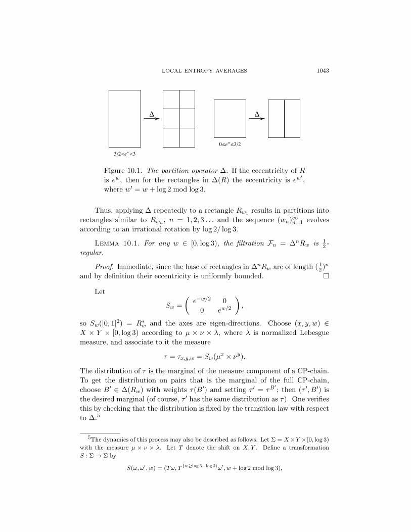
LOCAL ENTROPY AVERAGES 1043
D D
0£ew
£32
32<ew
<3
Figure 10.1. The partition operator ∆. If the eccentricity of R
is ew, then for the rectangles in ∆(R) the eccentricity is ew′,
where w′ = w + log 2 mod log 3.
Thus, applying ∆ repeatedly to a rectangle Rw1 results in partitions into
rectangles similar to Rwn , n = 1, 2, 3 . . . and the sequence (wn)∞n=1 evolves
according to an irrational rotation by log 2/ log 3.
Lemma 10.1. For any w ∈ [0, log 3), the filtration Fn = ∆nRw is 12 -
regular.
Proof. Immediate, since the base of rectangles in ∆nRw are of length (12)n
and by definition their eccentricity is uniformly bounded.
Let
Sw =
Çe−w/2 0
0 ew/2
å,
so Sw([0, 1]2) = R∗w and the axes are eigen-directions. Choose (x, y, w) ∈X × Y × [0, log 3) according to µ × ν × λ, where λ is normalized Lebesgue
measure, and associate to it the measure
τ = τx,y,w = Sw(µx × νy).
The distribution of τ is the marginal of the measure component of a CP-chain.
To get the distribution on pairs that is the marginal of the full CP-chain,
choose B′ ∈ ∆(Rw) with weights τ(B′) and setting τ ′ = τB′; then (τ ′, B′) is
the desired marginal (of course, τ ′ has the same distribution as τ). One verifies
this by checking that the distribution is fixed by the transition law with respect
to ∆.5
5The dynamics of this process may also be described as follows. Let Σ = X×Y × [0, log 3)
with the measure µ × ν × λ. Let T denote the shift on X,Y . Define a transformation
S : Σ→ Σ by
S(ω, ω′, w) = (Tω, T w≥log 3−log 2)ω′, w + log 2 mod log 3),
1044 MICHAEL HOCHMAN and PABLO SHMERKIN
Note that if µ and ν are ergodic, then Sw(µx × νy) almost surely has the
same dimension as θ = µ× ν.
Proposition 10.2. Suppose µ and ν are ergodic. For every ε > 0, there
is a subset Aε ⊆ [0, 1]2 with θ(Aε) > 1 − ε and a dense, open set Uε ⊆ Π2,1
such that for π ∈ Uε,
dim∗ π(θ|Aε) > min1,dim θ − ε.
Proof. Let P denote the distribution of the CP-chain, and write
α = min1,dim θ.
This is the expected dimension of the projection of a typical measure for a
typical ergodic component of the process. By Theorem 8.3 we can find a
dense open set U ′ε ⊆ Π2,1 and A′ε ⊆ P(Rd) such that P (A′ε) > 1 − ε, and
dim∗ πτ > α− ε for all π ∈ U ′ε and τ ∈ A′ε.Using the fact that, conditioned on w, the distribution of τ = τx,y,w is
Sw(µx × νy), with (x, y) ∼ θ, we can apply Fubini to find a w0 ∈ [0, log 3) and
a Borel set E ⊆ X × Y such that θ(E) > 1− ε and for every (x, y) ∈ E,
dim∗ π(Sw0µx × νy) > α− ε for all π ∈ U ′ε.
For an affine map S we identify π S with the projection π′ whose pre-image
sets partition R2 into the same lines as π S. Let
Uε = π Sw0 : π ∈ U ′ε.
Then Uε is open and dense in Π2,1 and for (x, y) ∈ E,
dim∗ π(µx × νy) > α− ε for all π ∈ Uε.
Define η ∈ P([0, 1]2) by
η =
∫Eµx × νy dθ(x, y).
Then by Lemma 3.1,
dim∗ πη > α− ε for all π ∈ Uε.
Since
θ = µ× ν =
∫µx × νy dθ(x, y),
we have η µ× ν, and since θ(E) > 1− ε, there is a subset Aε ⊆ [0, 1]2 such
that θ|Aε ∼ η and θ(Aε) > 1− ε. This is the desired set.
where Tσ = T if the event σ occurs and is the identity otherwise. This represents the
dynamics as a skew product X × [0, log 3) with fiber Y , in which the second coordinate w is
used to control the average speed with which the third coordinate (i.e., Y ) is advanced.
LOCAL ENTROPY AVERAGES 1045
10.3. Proof of Theorem 1.3. Let µ, ν be ergodic T2, T3-invariant measures
on [0, 1], respectively, such that dim∗ µ, dim∗ ν > 0. Let θ = µ× ν. Write
α = min1,dim θ,
and for ε > 0, let Vε ⊆ Π2,1 denote the set
Vε =
®π ∈ Π2,1 :
there exists A ⊆ [0, 1]2 with
θ(A) > 1− ε and dim∗ π(θ|A) > α− ε
´.
In the previous section we saw that the interior of Vε is open and dense in
Π2,1. We now establish some invariance. For this, it is convenient to represent
projections π ∈ Π2,1 by the slope of their image; i.e., πa projects onto the line
y = ax + b. (We cannot represent projection to the y-axis, but also do not
want to.) We note that this identification of Vε as a subset of R is consistent
with the topology on Π2,1.
Proposition 10.3. Vε is invariant under the action by multiplication of
the semigroup S = 3i
2j: i, j ∈ N ⊆ (N,×); i.e., if πa∈Vε, then π3a,πa/2∈Vε.
Proof. Suppose πa ∈ Vε, and let A ⊆ [0, 1]2 be a set of measure > 1 − εas in the definition of Vε.
Write T2 × id for the map [0, 1]2 → [0, 1]2 given by
(T2 × id)(x, y) = (T2x, y),
and let
A0 = (T2 × id)−1A ∩ ([0, 12)× [0, 1]),
A1 = (T2 × id)−1A ∩ ([12 , 1)× [0, 1]),
so (T2 × id)−1A = A0 ∪ A1. By the invariance properties of µ, ν we see that
µ× ν is invariant under T2 × id, so
µ× ν(A0 ∪A1) = µ× ν((T2 × id)−1A) > 1− ε.
Also, write
µ0 = µ|[0,1/2)×[0,1], µ1 = µ|[1/2,1]×[0,1].
Now, by invariance we have
(10.4) µ× ν = (T2µ0 × ν) + (T2µ1 × ν).
It follows that there are affine maps S0, S1 of R with
πa(µ× ν|A) = S0πa/2(µ0 × ν|A0) + S1πa/2(µ1 × ν|A1).
One way to see this is to note that the fibers of πa/2 are lines of slope −2/a
and are mapped under (x, y) 7→ (2x, y) to the fibers of πa, which have slope
−1/a.

1046 MICHAEL HOCHMAN and PABLO SHMERKIN
By assumption, dim∗ πa(µ×ν|A) > α−ε. Affine maps preserve dimension,
so
α− ε< dim∗ πa(µ× ν|A)
= min¶
dim∗ S0πa/2(µ0 × ν|A0),dim∗ S1πa/2(µ1 × ν|A1)©
= min¶
dim∗ πa/2(µ0 × ν|A0), dim∗ πa/2(µ1 × ν|A1)©
= dim∗ πa/2(µ× ν|(T2×id)−1A),
whence πa/2 ∈ Vε.A similar analysis, the measures νi = ν|[0,1]×[i/3,(i+1)/3) and the identity
µ× ν = T3(µ× ν0) + T3(µ× ν1) + T3(µ× ν2),
show that if πa ∈ Vε, then π3a ∈ Vε.
We can now conclude the proof of Theorem 1.3.
Proof of Theorem 1.3. Using (10.2) for µ, ν and Lemma 3.1 (2) applied to
π(µ× ν), the general case is reduced to the case in which µ and ν are ergodic.
Furthermore, by Corollary 3.9 it is enough to show that dim∗ π(µ× ν) ≥ α.
Since log 3/ log 2 /∈ Q, the semigroup
S =
®3i
2j: i, j ∈ N
´is dense in R+ [11]; this is the only place in the proof where we use the arith-
metic properties of m,n. For each ε > 0, we have seen that the interior of Vεis open and dense and, in particular, contains an open set in each of the rays
R+,R−; since it is invariant under S, we see that
Vε = πa : a 6= 0.
For any πa, a 6= 0, we have thus shown that there is a set Aε with µ× ν(Aε) >
1− ε and
dim∗ πa(µ× ν|Aε) > α− ε,which implies that
dim∗ π(µ× ν) ≥ α,as desired.
10.4. Proof of the topological conjecture. We briefly show how to derive
the topological version, Conjecture 1.1, from the measure one above. Suppose
that X,Y ⊆ [0, 1] are closed and invariant under T2, T3, respectively. Using
the variational principle (see, e.g., [33, Th. 14.1]), we can find probability
measures µ, ν on [0, 1), invariant and ergodic under T2, T3, respectively, such
that dimµ = dimA and dim ν = dimB.

LOCAL ENTROPY AVERAGES 1047
Let θ = µ × ν so that dim θ = dimA × B. For any projection π ∈Π2,1 \ πx, πy, we have by the theorem above that
dimπθ = min1, dim θ.
Since πθ is supported on π(A×B), we have
dimπ(A×B) ≥ min1, dim θ = min1,dim(A×B).
The right-hand side is also an upper bound, so we are done.
10.5. The Rudolph-Johnson theorem. In this section we show how The-
orem 1.3 implies the Rudolph-Johnson theorem. We first prove the theorem
under the hypothesis that the measure has positive dimension rather than
positive entropy of ergodic components.
Theorem 10.4. Let µ be a probability measure on [0, 1] that is invariant
under Tm and Tn, with m,n not powers of the same integer. Suppose that
dim∗ µ > 0. Then µ=Lebesgue measure.
Proof. Write α = dim∗ µ > 0. Denote by ∗ the convolution in R and
by the convolution in R/Z. Notice that, up to an affine map, µ ∗ µ and
π1(µ×µ) are the same. (Recall that π1 is projection to the line y = x.) Thus,
by Theorem 1.3 with µ = ν,
dim∗(µ ∗ ν) = dim∗ π1(µ× ν) = min1, 2α.
Also, since
µ µ = µ ∗ µ mod 1
and reduction modulo 1 is a countable-to-one local isometry,
dim∗(µ µ) = min1, 2α.
Finally, it is easy to check that µ µ is again invariant under Tm and Tn,
because Tm, Tn are endomorphisms of R/Z.
Iterating this argument, we see that for each k,
dim∗ µ µ · · · µ︸ ︷︷ ︸2k times
= min1, 2kα,
and since α > 0, there is a k so that, for ν = 2kµ,
dim∗ ν = 1.
But ν is a T2-invariant measure, and by (10.1) and (10.2) Lebesgue measure
is the only Tm invariant measure of lower dimension 1. Thus
ν = λ.

1048 MICHAEL HOCHMAN and PABLO SHMERKIN
To establish µ = λ, we look at the Fourier coefficients, where convolution
translates to multiplication. For i 6= 0, we have
µ(i)2k = ν(i) = λ(i) = 0.
Thus µ(i) = 0 for i 6= 0, so µ = λ.
For measures which are ergodic under Tm or even under the joint action
of Tm, Tn, positive dimension and positive entropy are equivalent conditions.
However, the condition that all ergodic components have positive entropy is
weaker; entropy behaves like the mean of the entropies of ergodic components,
while dimension behaves like the essential infimum. Nevertheless, there is a
simple reduction which recovers the nonergodic case.
Theorem 10.5 (Rudolph-Johnson [34], [19]). Let µ be a probability mea-
sure on [0, 1] that is invariant under Tm and Tn, with m,n not powers of the
same integer. Suppose that all ergodic components of µ with respect to Tm have
positive entropy. Then µ=Lebesgue measure.
Proof. Let µ =∫µωdν(ω) denote the ergodic decomposition of µ with
respect to Tm, where ν is defined on an auxiliary space Ω. Since Tn is an
endomorphism of ([0, 1], µ, Tm), it acts on the ergodic components, i.e., on
(Ω, ν), in a measure-preserving manner. Furthermore, since the joint action
of Tm, Tn on µ is ergodic, Tn acts ergodically on the space (Ω, ν) of ergodic
components.
Fix t > 0, let Ωt = ω ∈ Ω : h(Tm, µω) ≥ t, and let µ≥t =∫
Ωtµωdν(ω).
Since Tn is a factor map between ([0, 1], Tm, µω) and ([0, 1], Tm, Tnµω), and
since factor maps do not increase entropy, we have h(Tm, µω) ≥ h(Tm, Tnµω),
and therefore T−1n Ωt ⊆ Ωt. Since Tn is ν-preserving, Ωt is Tn-invariant up to
measure 0.
Hence µ≥t is Tn-invariant. It is also clearly Tm invariant, and its dimension
is
dim∗ µ≥t = essinfω∈Ωt
h(µω, Tm)
logm≥ t
logm> 0.
Hence by the previous theorem, µ≥t is Lebesgue measure. Since µ = limµ≥t,
we are done.
11. Convolutions of Gibbs measures
11.1. Preliminaries. Let I = fi : i ∈ Λ be an iterated function sys-
tem on the interval [0, 1]. The IFS I is called a regular IFS if the following
conditions hold:
(1) Regularity: There is ε > 0 such that each fi is a C1+ε map on a
neighborhood of [0, 1].
(2) Contraction and orientation: 0 < Dfi(x) < 1 for all i and all x ∈ [0, 1].
LOCAL ENTROPY AVERAGES 1049
(3) Separation: The sets fi((0, 1)) are pairwise disjoint subsets of (0, 1).
We say that a closed set X ⊆ [0, 1] is a regular Cantor set if it is the attractor
of a regular IFS. This definition is more restrictive than the one in, e.g., [26].
Our methods can handle the more general setting with slight modifications,
but for simplicity we concentrate on the case above.
We recall the definition and some basic facts about Gibbs measures; a
clearly written introduction to this topic can be found in [6, Ch. 5]. Let Λ be
a finite set. If ϕ : ΛN → R is a Holder-continuous function, then there exist a
unique real number P (ϕ) and a unique ergodic measure µϕ on ΛN such that
(11.1) µϕ([x1 · · ·xn]) = Θϕ
Ñexp
Ñ−nP (ϕ) +
n−1∑j=0
ϕ(T jx)
éé,
for all x ∈ ΛN, where T is the shift on ΛN. (Recall that A = Θϕ(B) means that
C−1A ≤ B ≤ CA for a constant C > 0 depending only on ϕ.) The number
P (ϕ) is known as the topological pressure of ϕ, and the measure µϕ as the
Gibbs measure for the potential ϕ.
We say that two measures defined on the same measure space are C-equi-
valent if they are mutually absolutely continuous and both Radon-Nikodym
derivatives are bounded by C; this is denoted by ∼C . If x, y are numbers, we
also write x ∼C y to denote that x ≤ Cy and y ≤ Cx.
Given a cylinder set [a] and a measure µ on ΛN, let µ[a] denote the prob-
ability measure on ΛN given by
µ[a]([b]) =1
µ([a])µ([ab]).
This is the symbolic analogue of rescaling a measure on Rd.While Gibbs measures are not generally product measures, they do satisfy
a slightly weaker property, which is the only one of their properties that we
use.
Lemma 11.1. Let µ be a Gibbs measure on ΛN for some Holder poten-
tial ϕ. Then there is C = C(ϕ) > 0 such that for any word a ∈ Λ∗, µ ∼C µ[a].
Proof. It follows from (11.1) that
µ[a][b] =µ[ab]
µ[a]= Θϕ(µ[b]).
This shows that µ[a] and µ are C-equivalent for some C that depends on ϕ
only.
Motivated by the previous lemma, we say that a measure µ on ΛN is a
C-quasi-product measure if C > 0 and µ[a] ∼C µ for all a ∈ Λ∗ or, equivalently,
C−1µ([ab]) ≤ µ([a])µ([b]) ≤ Cµ([ab]).

1050 MICHAEL HOCHMAN and PABLO SHMERKIN
A few comments about this notion are in order. It is easy to see that
the support of a quasi-product measure on ΛN is ΞN for some subset Ξ ⊆ Λ.
Thus by replacing Λ by Ξ, we can always assume that quasi-product mea-
sures are globally supported. Each Tnµ is C-equivalent to µ, and taking any
weak-* limit point ν of 1n
(µ+ Tµ+ T 2µ+ · · ·+ Tn−1µ
), as n → ∞, we ob-
tain a T -invariant measure equivalent to µ and with Radon-Nikodym derivative
bounded between C−1 and C. Also, it is easy to show that µ has a rudimen-
tary mixing property. There is a constant K such that if A,B are sets then
µ(T−nA ∩ B)>Kµ(A)µ(B) for large enough n. It follows that the same is
true of ν, perhaps with a different constant, and so ν is ergodic. It follows now
that ν, and hence µ, are exact dimensional.
Finally, we transfer these notions to the geometric attractor. A Gibbs
measure on X is the projection of a Gibbs measure on ΛN under the coding
map. In the same way we define quasi-product measures on X. Thus, Gibbs
measures on X are quasi-product measures.
We have the following slight strengthening of Theorem 1.4.
Theorem 11.2. Theorem 1.4 holds for quasi-product measures µi on the
attractors Xi.
For notational simplicity we prove Theorem 11.2 for d = 2; the proof is
the same in higher dimensions. The structure of the proof resembles that of
Theorem 1.6, but is technically more difficult. The main differences are, first,
that micromeasures of Gibbs measures on regular IFSs are harder to relate
to the original measure and, second, that moving the open set around Π2,1 is
more involved due to nonlinearity of the IFSs. In the next section we present
some standard tools for dealing with these problems.
Before embarking on the proof we explain its relation to Moreira’s proof
of (1.4) in the strictly nonlinear case. The key device there was the so-called
Scale Recurrence Lemma (SRL) of [26]. This technical result, which relies on
the nonlinearity of the system, gives information about the quotients
diam(f(1)a ([0, 1]))
diam(f(2)b ([0, 1]))
for many (but not all) pairs a ∈ Λ∗1, b ∈ Λ∗2. In the proof one uses only the pairs
of words that are “good” in the sense of the SRL in order to construct subsets
X ′i ⊆ Xi that approximate Xi well in dimension, but have zero measure with
respect to any Gibbs measure. Hence it seems unlikely that Moreira’s proof
can be adapted to give information about convolutions of Gibbs measures. Our
proof uses the machinery of CP processes in place of the SRL, specifically in
the proof of Proposition 11.8. After that our proof follows Moreira’s original
argument.

LOCAL ENTROPY AVERAGES 1051
11.2. Limit geometries and micromeasures. Throughout this subsection,
I = fi : i ∈ Λ is a regular IFS with attractor X and µ is a C-quasi-product
measure on X. By definition, µ = Φη, where Φ is the coding map and η is a
C-quasi-product measure on ΛN.
Given a closed interval [a, b], denote by T[a,b] the unique orientation-
preserving affine map sending [a, b] to [0, 1]. If f : [0, 1] → R is a continuous
injection, write
Tf = Tf([0,1])
and
f∗ = Tff.
Hence f∗ is a bijection of [0, 1]. Also, for a ∈ Λ∗, write
I(a) = fa([0, 1]).
The following simple lemma is a consequence of the separation assumption on
the IFS and C-equivalence.
Lemma 11.3. For every a ∈ Λ∗,
µI(a) ∼C fa(µ).
Proof. For any b ∈ Λ∗,
µI(a)(I(ab)) =µ(I(ab))
µ(I(a))∼C µ(I(b)) = (faµ) (I(ab)).
Since I(ab) is a basis of closed sets of X ∩ I(a), this yields the lemma.
The following result goes back to Sullivan [35], with an explicit proof
given by Bedford and Fisher [2]. It will be a key tool in the proof, in particular
allowing us to describe the micromeasures of a Gibbs measure.
Theorem 11.4. For every left-infinite sequence x = (. . . x−2x−1), the se-
quence of rescaled diffeomorphisms (fx−n · · · fx−1)∗ converges in the C1 topology
to a diffeomorphism Fx : [0, 1]→ [0, 1], uniformly in x. In particular, the map
x 7→ Fx is continuous.
In this case, the sets Fx(X) are known as limit geometries of X. We also
refer to the maps Fx themselves as limit diffeomorphisms.
Heuristically, the reason for the validity of Sullivan’s Theorem is the fol-
lowing. When composing fx−n · · · fx−1 , the strongest nonlinear distortion
comes from the first map applied, fx−1 . Since each map is a contraction, fx−iis applied to an interval of length exponentially small in i. As i gets large,
the nonlinear effect of fx−i becomes negligible. (The details of this argument
require C1+ε-regularity of the contractions.)
Note that when the contractions are similarities the maps Fa are all the
identity, and Sullivan’s Theorem becomes trivial.

1052 MICHAEL HOCHMAN and PABLO SHMERKIN
If x ∈ Λ−N, one may consider the conjugated IFS
Ix = FxfiF−1x : i ∈ Λ,
whose attractor is the limit geometry Fx(X). More generally, if Φx is the
coding map for Ix, then Φx = FxΦ.
Corollary 11.5. (i) Choose a ∈ Λ∗, and write a = (. . . aa) ∈ Λ−N.
Then FafaF−1a is an affine map, and λ(FafaF
−1a ) = λ(fa). (Recall
(1.3) for the definition of λ(·).)(ii) Let g ∈ C1([0, 1],R), and consider the conjugated IFS I ′ = gfig−1 :
i ∈ Λ. Then for any x ∈ Λ−N, Ix = I ′x. In particular, this holds when
g is itself a limit diffeomorphism Fy .
Proof. (i) Write Tn = Tfan , where an is the n-fold concatenation of a. We
have
FafaF−1a = lim
nTnfanfaF
−1a
= limn
ÄTnT
−1n+1
äTn+1fan+1F−1
a
= limnTnT
−1n+1,
which is affine as a limit of affine maps. The last assertion follows since λ(·) is
conjugacy-invariant.
(ii) Limit diffeomorphisms are clearly invariant under affine changes of
coordinates and, being an infinitesimal property of the IFS, therefore also
under smooth changes of coordinates.
Next, we state a well-known consequence of the principle of bounded dis-
tortion, which can be easily deduced from Theorem 11.4. For the rest of the
section, the constants implicit in the O(·) notation depend only on the IFSs
involved.
Proposition 11.6. Let I = fi : i ∈ Λ be a regular IFS. Then for any
finite word a ∈ Λ∗ and any i, j ∈ Λ,
dist(I(ai), I(aj)) = Θ(|I(a)|)
and
|I(ai)| = Θ(|I(a)|).
The next step is to relate µ to its micromeasures. Recall that the family
of micromeasures of a measure η on Rk is denoted 〈η〉. The following theorem
is analogous to Proposition 9.1.

LOCAL ENTROPY AVERAGES 1053
Proposition 11.7. For any ν ∈ 〈µ〉 which is not supported on 0, 1,there is a limit diffeomorphism F and an interval J such that
Fµ ∼C νJ .
Proof. By definition, there are intervals In ⊆ [0, 1] such that
ν = limn→∞
µIn ,
where µI = TI(µI) is the rescaling of µI back to the unit interval. For each
n, let a(n) be a minimal word such that I(a(n)) ⊆ In. (There could be several
such words; pick one of them.) Since ν is not supported on 0, 1, this is well
defined for large n, and moreover |In| = O(|I(a(n))|) by bounded distortion
(i.e., Proposition 11.6).
By Lemma 11.3, writing fn = fa(n) ,
µI(a(n)) ∼C f∗nµ.
On the other hand, for each n there is an interval Jn (corresponding to the
relative position of I(a(n)) inside In) such that |Jn| = Θ(1), and
µI(a(n)) = TJn((µIn)Jn).
By passing to a subsequence we can assume that TJn converges to an affine
map TJ and f∗n to a limit diffeomorphism F . Taking weak limits yields the
proposition.
11.3. Proof of Theorem 11.2. Throughout this section, µ1, µ2 are quasi-
product measures associated to regular IFSs Ii = f (i)j : j ∈ Λi, i = 1, 2. We
write µ = µ1 × µ2 and
γ = min(1, dimµ).
We say that F : [0, 1]2 → [0, 1]2 is a limit diffeomorphism if F = F1×F2, where
Fi is a limit diffeomorphism for Ii.We next state the main three steps in the proof of Theorem 11.2. The
first one is, as usual, a topological version of the projection theorem, which
does not require any minimality assumptions; compare with Proposition 9.3.
Given a measure ν on Rd and α ≥ 0, let
(11.2) Uα(ν) = interiorg ∈ C1(supp ν,Rk) : dim∗ gν > α.
Note that these sets are by definition open, though a priori may be empty.
Proposition 11.8. For every ε > 0, there exists a limit diffeomorphism
F such that
Uγ−ε(Fµ) contains a dense (and automatically open) subset of Π2,1.

1054 MICHAEL HOCHMAN and PABLO SHMERKIN
Identify Π2,1\πx, πy with R\0 via s→ πs(x, y) = x+ sy. (The latter
is not technically an element of Π2,1 but there is an obvious identification.)
This is similar but not the same as the identification in Section 10. Given
K 1, writeIK = [−K,−K−1] ∪ [K−1,K].
Using the irreducibility assumption to move the open and dense set around as
usual (but with some extra technical complications), one obtains
Proposition 11.9. If, in addition, the minimality condition in Theo-
rem 1.4 holds, then for every ε > 0 and every K > 1, there is a limit diffeo-
morphism F such that
πs : s ∈ IK ⊆ Uγ−ε(Fµ).
A priori, this holds for just one limit diffeomorphism F = F1 × F2. But
this automatically implies, it holds in fact for all limit diffeomorphisms.
Proposition 11.10. Under the hypotheses of Proposition 11.9, for every
ε > 0, every K > 1, and every limit diffeomorphism F ,
πs : s ∈ IK ⊆ Uγ−ε(Fµ).
Before proving these propositions we use them to deduce Theorem 11.2.
We say that a map A : R2 → R2 is affine diagonal if it is affine with
a diagonal linear part. In this case, we can write A = HD, where H is
an homothety and D(x, y) = (x, ay) for some a ∈ R. We refer to a as the
eccentricity of A.
Lemma 11.11. Let ν, τ be two measures on Rd, and suppose that Aν ∼CτQ for some affine diagonal map A and some set Q with τ(Q) > 0. Then for
any α,Uα(ν) ⊇ gA : g ∈ Uα(τ),
Uα(ν) ∩Π2,1 ⊇ πsa : πs ∈ Uα(τ),
where a is the eccentricity of A.
Proof. The first part is immediate. For the second, note that if D(x, y) =
(x, ay), then πsD = πas, and note that homotheties commute with linear maps
and preserve dimension.
Proof of Theorem 11.2 (assuming Proposition 11.10). By Corollary 3.9, it
is enough to show that
dim∗(π(µ1 × µ2)) ≥ γ.Fix ε > 0 and K > 1 for the rest of the proof. For i = 1, 2, let x(i) ∈ Λ−Ni , and
write Fi = Fx(i) , F = F1 × F2. Since, by Proposition 11.10,
(11.3) πs : s ∈ IK ⊆ Uγ−ε(Fµ),

LOCAL ENTROPY AVERAGES 1055
we have by compactness of IK and openness of Uγ−ε(Fµ) that the same is true
if one replaces F by a sufficiently close diffeomorphism. Since the convergence
of f∗yn···y1 to Fy is uniform, it follows that that for sufficiently long initial
segments a1, a2 of x(1), x(2) (where the threshold length is also independent of
x(i)), if we write f∗ = f∗a1 × f∗a2 , then (11.3) holds with f∗µ instead of Fµ.
By the principle of bounded distortion, we can choose the lengths of ai such
that I(a1), I(a2) have lengths which differ by a factor of O(1), and still ensure
that the length of both is bounded above independently of other parameters.
Consider now the affine diagonal map A = TI(a1) × TI(a2); i.e., A is such that
f∗ = Af , where f = fa1 × fa2 . By construction the eccentricity of A is O(1).
Since A(fµ) = f∗µ, we get from Lemma 11.11 that
πs : s ∈ IK/O(1) ⊆ Uγ−ε(fµ).
Recall that fµ ∼C µI(a1)×I(a2) by the quasi-product property. We may cover
supp(µ) by rectangles of the form I(a1)× I(a2), with a1, a2 chosen to be long
enough for the above to hold. Thus, since ε and K were arbitrary, the proof
is complete.
11.4. Proofs of the remaining propositions.
Proof of Proposition 11.8. The proof is analogous to the proof of Propo-
sition 9.3. We apply Theorem 7.10 to obtain an ergodic CP-chain (µn, Qn)∞n=1
such that almost surely µ1 ∈ 〈µ〉 and dimµ1 = dimµ. Hence, we can find a
micromeasure ν such that dim ν ≥ dimµ, and the conclusion of Corollary 8.5
applies to ν; given ε > 0, the family Uγ−ε(ν) has dense intersection with Π2,1.
By compactness, ν = ν1 × ν2, where νi ∈ 〈µi〉. By Proposition 11.7, we
can find a limit diffeomorphism F , an affine diagonal map A and a rectangle
Q, such that Aµ ∼C νQ. The proposition then follows from Lemma 11.11.
For the proof of Proposition 11.9, we need the following lemma.
Lemma 11.12. Suppose U ⊆ R \ 0 and
πs : s ∈ U ⊆ Uα(µ).
Then for any limit diffeomorphism F , there is a t = t(F ) = Θ(1) such that
πts : s ∈ U ⊆ Uα(Fµ).
Proof. This is very similar to the proof of Theorem 11.2 above. One uses
the fact that, up to affine rescaling and C-equivalence, the limit measure Fµ is
C1-close to the restriction of µ to a small rectangleQ of eccentricity Θ(1). Since
Uα(µQ) ⊇ Uα(µ), and the rescaling induced on Π2,1 by pre-composition with
TQ transforms πs to πts, where t is the eccentricity of Q, the lemma follows by
applying this procedure to a sequence of rectangles Qn of side length tending
to 0 and eccentricities converging to some t = Θ(1).

1056 MICHAEL HOCHMAN and PABLO SHMERKIN
Proof of Proposition 11.9. To begin, note that a priori we cannot “move
around” the dense set given by Proposition 11.8 as done in, e.g., Proposi-
tion 9.4, since for this we need the action of an affine map and the IFSs
involved are a priori nonlinear. Instead we linearize the relevant map in each
IFS by passing to a new limit geometry.
We first present the proof in the case λ(f(1)a1 )/λ(f
(2)a2 ) /∈ Q for some ai ∈ Λ∗i .
By iterating the IFSs and relabeling, we may then assume that λ(f(1)1 )/λ(f
(2)1 )
/∈ QLet F = F1 × F2 be the limit diffeomorphism given by Proposition 11.8.
The conjugated IFS I ′i = Fif (i)j F−1
i : j ∈ Λi satisfies the same hypotheses
as the original one. Let x = (. . . , 1, 1) ∈ Λ−Ni . By Corollary 11.5(i), the first
map in each limit IFS (Ii)x is affine. But by Corollary 11.5(ii), (Ii)x = (I ′i)x.
On the other hand, by Lemma 11.12, the conclusion of Proposition 11.8 is
inherited by (I ′i)x. We have therefore shown that there is no loss of generality
in assuming that the conjugated IFSs g(i)j = Fif
(i)j F−1
i : j ∈ Λi are such that
g(1)1 , g
(2)1 are affine. Moreover, we still have
(11.4) λ(g
(1)1
)/λ(g
(2)1
)/∈ Q.
Now we are ready to cover the whole of IK by using the action of g(1)1 × g(2)
1
on Uγ−ε(Fµ). By (11.4), the collection of eccentricities of the (affine diagonal)
maps
gn1,n2 :=(g
(1)1
)n1
×(g
(2)1
)n2
is dense in (0,∞). Also note that
g−1n1,n2
(Fµ)Qn1,n2 ∼C Fµ,
where Qn1,n2 = gn1,n2([0, 1]2). It then follows from Lemma 11.11 that there is
N such that
πs : s ∈ IK ⊆N⋃
n1,n2=1
Uγ−ε((Fµ)Qn1,n2 ).
Pick N1, N2 ≥ N such that the eccentricity of gN1,N2 is less than, say, 2. By the
above, Uγ−ε((Fµ)QN1,N2) contains πs : s ∈ IK. But then using Lemma 11.11
again we conclude that Uγ−ε(Fµ) contains πs : s ∈ IK/2, as desired.
In the general case we can still, by minimality and Proposition 11.8, find
ai ∈ Λ∗i , i = 1, 2, and an N such that
IK ⊆N⋃
n1,n2=1
λÄf (1)a1
än1λÄf (2)a2
ä−n2t : πt ∈ Uγ−ε(Fµ)
.
By Lemma 11.12, the same holds after passing to the limit IFSs which lin-
earize the maps f(i)ai , at the cost of replacing IK by IΩ(K). The argument then
proceeds in the same manner as before.

LOCAL ENTROPY AVERAGES 1057
Proof of Proposition 11.10. By Lemma 11.12, if the set Uα(µ) contains
πs : s ∈ IK, then the same is true with K replaced by Ω(K) and µ replaced
by Fµ for any limit diffeomorphism F . We know that Uα(Gµ) contains IKfor some limit diffeomorphism G. Thus Corollary 11.5(ii) and the previous
observation applied to the conjugated IFSs Gif (i)j G−1
i : i ∈ Λi (i.e., to the
measure Gµ) yield the result.
Acknowledgement. This project began during the program “Ergodic the-
ory and additive combinatorics” at MSRI, and we are grateful to the organizers
and MSRI for the stimulating atmosphere. We also thank Yuval Peres for use-
ful comments and particularly for suggesting a simplification to the proof of
Lemma 4.3.
References
[1] T. Bedford and A. M. Fisher, On the magnification of Cantor sets and their
limit models, Monatsh. Math. 121 (1996), 11–40. MR 1375638. Zbl 0843.28002.
http://dx.doi.org/10.1007/BF01299636.
[2] , Ratio geometry, rigidity and the scenery process for hyperbolic Can-
tor sets, Ergodic Theory Dynam. Systems 17 (1997), 531–564. MR 1452179.
Zbl 0886.58089. http://dx.doi.org/10.1017/S0143385797079194.
[3] T. Bedford, A. M. Fisher, and M. Urbanski, The scenery flow for hyperbolic
Julia sets, Proc. London Math. Soc. 85 (2002), 467–492. MR 1912058. Zbl 1014.
37034. http://dx.doi.org/10.1112/S002461150201362X.
[4] T. M. Cover and J. A. Thomas, Elements of Information Theory, second ed.,
Wiley-Interscience [John Wiley & Sons, Inc.], Hoboken, NJ, 2005. MR 2239987.
Zbl 1140.94001. http://dx.doi.org/10.1002/047174882X.
[5] K. Falconer, Fractal Geometry, Mathematical Foundations and Applications,
John Wiley & Sons Ltd., Chichester, 1990. MR 1102677. Zbl 0689.28003.
[6] , Techniques in Fractal Geometry, John Wiley & Sons Ltd., Chichester,
1997. MR 1449135. Zbl 0869.28003.
[7] A.-H. Fan, K.-S. Lau, and H. Rao, Relationships between different dimensions
of a measure, Monatsh. Math. 135 (2002), 191–201. MR 1897575. Zbl 0996.
28001. http://dx.doi.org/10.1007/s006050200016.
[8] W. Feller, An Introduction to Probability Theory and its Applications. Vol. II.,
second ed., John Wiley & Sons, Inc., New York, 1971. MR 0270403. Zbl 0219.
60003.
[9] D.-J. Feng and H. Hu, Dimension theory of iterated function systems, Comm.
Pure Appl. Math. 62 (2009), 1435–1500. MR 2560042. Zbl 05614742. http://dx.
doi.org/10.1002/cpa.20276.
[10] A. Ferguson, T. Jordan, and P. Shmerkin, The Hausdorff dimension of the
projections of self-affine carpets, Fund. Math. 209 (2010), 193–213. MR 2720210.
Zbl 1206.28011. http://dx.doi.org/10.4064/fm209-3-1.

1058 MICHAEL HOCHMAN and PABLO SHMERKIN
[11] H. Furstenberg, Disjointness in ergodic theory, minimal sets, and a problem in
Diophantine approximation, Math. Systems Theory 1 (1967), 1–49. MR 0213508.
Zbl 0146.28502. http://dx.doi.org/10.1007/BF01692494.
[12] , Intersections of Cantor sets and transversality of semigroups, in Problems
in Analysis (Sympos. Salomon Bochner, Princeton Univ., Princeton, N.J., 1969),
Princeton Univ. Press, Princeton, N.J., 1970, pp. 41–59. MR 0354562. Zbl 0208.
32203.
[13] , Ergodic fractal measures and dimension conservation, Ergodic Theory
Dynam. Systems 28 (2008), 405–422. MR 2408385. Zbl 1154.37322. http://dx.
doi.org/10.1017/S0143385708000084.
[14] M. Gavish, Measures with uniform scaling scenery, Ergodic Theory Dynam.
Systems 31 (2011), 33–48. MR 2755920. Zbl 1225.37012. http://dx.doi.org/10.
1017/S0143385709000996.
[15] J. Gonzalez Llorente and A. Nicolau, Regularity properties of mea-
sures, entropy and the law of the iterated logarithm, Proc. London Math. Soc.
89 (2004), 485–524. MR 2078701. Zbl 1058.60029. http://dx.doi.org/10.1112/
S0024611504014844.
[16] S. Graf, On Bandt’s tangential distribution for self-similar measures, Monatsh.
Math. 120 (1995), 223–246. MR 1363139. Zbl 0841.28011. http://dx.doi.org/
10.1007/BF01294859.
[17] M. Hochman, Dynamics on fractal measures, 2010, preprint. arXiv 1008.3731.
[18] B. R. Hunt and V. Y. Kaloshin, How projections affect the dimension spec-
trum of fractal measures, Nonlinearity 10 (1997), 1031–1046. MR 1473372.
Zbl 0903.28008. http://dx.doi.org/10.1088/0951-7715/10/5/002.
[19] A. S. A. Johnson, Measures on the circle invariant under multiplication by a
nonlacunary subsemigroup of the integers, Israel J. Math. 77 (1992), 211–240.
MR 1194793. Zbl 0790.28012. http://dx.doi.org/10.1007/BF02808018.
[20] A. Kaenmaki, T. Rajala, and V. Suomala, Local homogeneity and dimen-
sions of measures in doubling metric spaces, 2010, preprint. arXiv 1003.2895.
[21] R. Kenyon, Projecting the one-dimensional Sierpinski gasket, Israel J. Math.
97 (1997), 221–238. MR 1441250. Zbl 0871.28006. http://dx.doi.org/10.1007/
BF02774038.
[22] D. Krieg and P. Morters, Tangent measure distributions of hyperbolic Cantor
sets, Monatsh. Math. 126 (1998), 313–328. MR 1657810. Zbl 0935.28001. http:
//dx.doi.org/10.1007/BF01299055.
[23] E. Lindenstrauss, D. Meiri, and Y. Peres, Entropy of convolutions on the
circle, Ann. of Math. 149 (1999), 871–904. MR 1709305. Zbl 0940.28015. http:
//dx.doi.org/10.2307/121075.
[24] P. Mattila, Geometry of Sets and Measures in Euclidean Spaces. Fractals
and Rectifiability, Cambridge Stud. Adv. Math. 44, Cambridge Univ. Press,
Cambridge, 1999. MR 1333890. Zbl 0819.28004. http://dx.doi.org/10.2277/
0521655951.
[25] C. G. T. de a. Moreira, Sums of regular Cantor sets, dynamics and applica-
tions to number theory, in International Conference on Dimension and Dynamics

LOCAL ENTROPY AVERAGES 1059
(Miskolc, 1998), 37 Period. Math. Hungar. no. 1-3, 1998, pp. 55–63. MR 1719468.
Zbl 0980.54025. http://dx.doi.org/10.1023/A:1004726319127.
[26] C. G. T. de a. Moreira and J.-C. Yoccoz, Stable intersections of regular
Cantor sets with large Hausdorff dimensions, Ann. of Math. 154 (2001), 45–96.
MR 1847588. Zbl 1195.37015. http://dx.doi.org/10.2307/3062110.
[27] P. Morters, Symmetry properties of average densities and tangent measure
distributions of measures on the line, Adv. in Appl. Math. 21 (1998), 146–179.
MR 1623341. Zbl 0914.28002. http://dx.doi.org/10.1006/aama.1998.0592.
[28] P. Morters and D. Preiss, Tangent measure distributions of fractal measures,
Math. Ann. 312 (1998), 53–93. MR 1645950. Zbl 0945.28002. http://dx.doi.org/
10.1007/s002080050212.
[29] F. Nazarov, Y. Peres, and P. Shmerkin, Convolutions of Cantor measures
without resonance, Israel J. Math. 187 (2012), 93–116. http://dx.doi.org/10.
1007/s11856-011-0164-8.
[30] Y. Peres, W. Schlag, and B. Solomyak, Sixty years of Bernoulli convolu-
tions, in Fractal Geometry and Stochastics, II (Greifswald/Koserow, 1998), Progr.
Probab. 46, Birkhauser, Basel, 2000, pp. 39–65. MR 1785620. Zbl 0961.42006.
[31] Y. Peres and P. Shmerkin, Resonance between Cantor sets, Ergodic Theory
Dynam. Systems 29 (2009), 201–221. MR 2470633. Zbl 1159.37005. http://dx.
doi.org/10.1017/S0143385708000369.
[32] Y. Peres and B. Solomyak, Existence of Lq dimensions and entropy dimen-
sion for self-conformal measures, Indiana Univ. Math. J. 49 (2000), 1603–1621.
MR 1838304. Zbl 0978.28004. http://dx.doi.org/10.1512/iumj.2000.49.1851.
[33] M. Pollicott and M. Yuri, Dynamical Systems and Ergodic Theory, Lon-
don Math. Soc. Student Texts 40, Cambridge Univ. Press, Cambridge, 1998.
MR 1627681. Zbl 0897.28009.
[34] D. J. Rudolph, ×2 and ×3 invariant measures and entropy, Ergodic Theory
Dynam. Systems 10 (1990), 395–406. MR 1062766. Zbl 0709.28013. http://dx.
doi.org/10.1017/S0143385700005629.
[35] D. Sullivan, Differentiable structures on fractal-like sets, determined by intrinsic
scaling functions on dual Cantor sets, in The Mathematical Heritage of Hermann
Weyl (Durham, NC, 1987), Proc. Sympos. Pure Math. 48, Amer. Math. Soc.,
Providence, RI, 1988, pp. 15–23. MR 0974329. Zbl 0665.58027.
[36] P. Walters, An Introduction to Ergodic Theory, Grad. Texts Math. 79,
Springer-Verlag, New York, 1982. MR 0648108. Zbl 0475.28009.
(Received: October 13, 2009)
(Revised: June 2, 2011)
Princeton University, Princeton, NJ
Current address : Einstein Institute of Mathematics, The Hebrew University
of Jerusalem, Jerusalem, Israel
E-mail : [email protected]
University of Surrey, Guildford, UK
E-mail : [email protected]