The quantitative behaviour of polynomial orbits on...
76
Annals of Mathematics 175 (2012), 465–540 http://dx.doi.org/10.4007/annals.2012.175.2.2 The quantitative behaviour of polynomial orbits on nilmanifolds By Ben Green and Terence Tao Abstract A theorem of Leibman asserts that a polynomial orbit (g(n)Γ) n∈Z on a nilmanifold G/Γ is always equidistributed in a union of closed sub- nilmanifolds of G/Γ. In this paper we give a quantitative version of Leib- man’s result, describing the uniform distribution properties of a finite poly- nomial orbit (g(n)Γ) n∈[N] in a nilmanifold. More specifically we show that there is a factorisation g = εg 0 γ, where ε(n) is “smooth,” (γ(n)Γ) n∈Z is periodic and “rational,” and (g 0 (n)Γ)n∈P is uniformly distributed (up to a specified error δ) inside some subnilmanifold G 0 /Γ 0 of G/Γ for all suffi- ciently dense arithmetic progressions P ⊆ [N ]. Our bounds are uniform in N and are polynomial in the error tolerance δ. In a companion paper we shall use this theorem to establish the M¨obius and Nilsequences conjecture from an earlier paper of ours. 1. Introduction Nilmanifolds. In the last few years it has come to be appreciated that nilmanifolds, together with orbits on them, play a fundamental role in combi- natorial number theory. Their relevance was certainly apparent in [7] and has been displayed quite dramatically in recent ergodic-theoretic work of Host-Kra [15] and Ziegler [35]. More recently the authors have explored how nilmanifolds arise in additive combinatorics [9] and in the study of linear equations in the primes [11]. The present paper is a part of that programme (and in particular will be used to prove the M¨obius and Nilsequences conjecture from [11] in the companion [12] to this paper) but, since it concerns only the intrinsic proper- ties of nilmanifolds, may be read independently of any of the other work. The reader interested in the background may consult the surveys [8], [17], [31], or the paper [11]. We begin by setting out our notation for nilmanifolds. The first author is a Clay Research Fellow and gratefully acknowledges the support of the Clay Institute. The second author is supported by a grant from the MacArthur Foundation. 465
Transcript of The quantitative behaviour of polynomial orbits on...

Annals of Mathematics 175 (2012), 465–540http://dx.doi.org/10.4007/annals.2012.175.2.2
The quantitative behaviour ofpolynomial orbits on nilmanifolds
By Ben Green and Terence Tao
Abstract
A theorem of Leibman asserts that a polynomial orbit (g(n)Γ)n∈Z on
a nilmanifold G/Γ is always equidistributed in a union of closed sub-
nilmanifolds of G/Γ. In this paper we give a quantitative version of Leib-
man’s result, describing the uniform distribution properties of a finite poly-
nomial orbit (g(n)Γ)n∈[N ] in a nilmanifold. More specifically we show that
there is a factorisation g = εg′γ, where ε(n) is “smooth,” (γ(n)Γ)n∈Z is
periodic and “rational,” and (g′(n)Γ)n∈P is uniformly distributed (up to
a specified error δ) inside some subnilmanifold G′/Γ′ of G/Γ for all suffi-
ciently dense arithmetic progressions P ⊆ [N ].
Our bounds are uniform inN and are polynomial in the error tolerance δ.
In a companion paper we shall use this theorem to establish the Mobius
and Nilsequences conjecture from an earlier paper of ours.
1. Introduction
Nilmanifolds. In the last few years it has come to be appreciated that
nilmanifolds, together with orbits on them, play a fundamental role in combi-
natorial number theory. Their relevance was certainly apparent in [7] and has
been displayed quite dramatically in recent ergodic-theoretic work of Host-Kra
[15] and Ziegler [35]. More recently the authors have explored how nilmanifolds
arise in additive combinatorics [9] and in the study of linear equations in the
primes [11]. The present paper is a part of that programme (and in particular
will be used to prove the Mobius and Nilsequences conjecture from [11] in the
companion [12] to this paper) but, since it concerns only the intrinsic proper-
ties of nilmanifolds, may be read independently of any of the other work. The
reader interested in the background may consult the surveys [8], [17], [31], or
the paper [11].
We begin by setting out our notation for nilmanifolds.
The first author is a Clay Research Fellow and gratefully acknowledges the support of the
Clay Institute. The second author is supported by a grant from the MacArthur Foundation.
465

466 BEN GREEN and TERENCE TAO
Definition 1.1 (Filtrations and nilmanifolds). Let G be a connected, sim-
ply connected Lie group with identity element idG. For the purposes of this
paper we define a filtration G• on G to be a sequence of closed connected
subgroups
G = G0 = G1 ⊇ G2 ⊇ · · · ⊇ Gd ⊇ Gd+1 = idGwhich has the property that [Gi, Gj ] ⊆ Gi+j for all integers i, j > 0. The
least integer d for which Gd+1 = idG is called the degree of the filtration
G• and here, as usual, the commutator group [H,K] is the group generated
by [h, k] : h ∈ H, k ∈ K, where [h, k] := hkh−1k−1 is the commutator of h
and k. If G possesses a filtration, then we say that G is nilpotent. Let Γ ⊆ G be
a uniform subgroup (i.e., a discrete, cocompact subgroup). Then the quotient
G/Γ = gΓ : g ∈ G is called a nilmanifold. We also write g(mod Γ) for gΓ.
Throughout the paper we will write m = dimG and mi = dimGi, i =
1, . . . , d.
Remark. The assumptions of connectedness and simple-connectedness for
G are not completely standard, but are very convenient for us. In any situation
in which we apply our theorems, we expect to be able to reduce to this case.
If a filtration G• of degree d exists, then it is easy to see that the lower central
series filtration1 defined by G = G0 = G1, Gi+1 = [G,Gi] terminates with
Gs+1 = idG for some integer s 6 d. We call the minimal such integer s the
step of the nilpotent Lie group G. In this paper the degree d will play a vastly
more important role than the step s, since it will be important to work with
filtrations more general than the lower central series.
Examples. The simplest examples of nilmanifolds arise when s = 1 in
which case we may, after a linear transformation, take G = Rm and Γ =
Zm. The lower central series filtration is given by G = G0 = G1 and G2 =
idG. The nilmanifold G/Γ is then referred to as a torus. Note that in this
example the group operation is written additively, as is conventional for abelian
groups. When we are working with non-abelian groups we shall write the group
operation multiplicatively. The simplest non-abelian example is given by the 3-
dimensional Heisenberg nilmanifold, in which s = 2. We will study this object
in some detail later on. Here we take
(1.1) G =(
1 R R0 1 R0 0 1
)and Γ =
(1 Z Z0 1 Z0 0 1
).
The lower central series filtration is given by G = G0 = G1,
G2 =(
1 0 R0 1 00 0 1
),
1It is not hard to see that the lower central series filtration is a filtration, in that we have
[Gi, Gj ] ⊆ Gi+j for all i, j.

THE BEHAVIOUR OF POLYNOMIAL ORBITS ON NILMANIFOLDS 467
and G3 = idG. Observe that a fundamental domain for the action of Γ on
G is
(1.2)
ßÅ1 x1 x20 1 x30 0 1
ã: 0 6 x1, x2, x3 < 1
™.
Thus one can view G/Γ as a unit cube, with the sides glued together in a
twisted fashion.
This paper will be concerned with the qualitative and quantitative equidis-
tribution of various algebraic sequences on nilmanifolds. We first set out our
notation for equidistribution.
Definition 1.2 (Equidistribution). Let G/Γ be a nilmanifold. Here and in
the sequel we endow G/Γ with the unique normalised Haar measure, we let
[N ] := n ∈ Z : 1 6 n 6 N, and we write Ea∈Af(a) := 1|A|∑a∈A f(A) for the
average of f on the set A.
(i) An infinite sequence (g(n)Γ)n∈N in G/Γ is said to be equidistributed if
we have
limN→∞
En∈[N ]F (g(n)Γ) =
∫G/Γ
F
for all continuous functions F : G/Γ→ C.
(ii) An infinite sequence (g(n)Γ)n∈Z in G/Γ is said to be totally equidis-
tributed if the sequences (g(an + r)Γ)n∈N are equidistributed for all
a ∈ Z\0 and r ∈ Z.
(iii) Given a length N > 0 and an error tolerance δ > 0, a finite sequence
(g(n)Γ)n∈[N ] is said to be δ-equidistributed if we have∣∣∣∣∣En∈[N ]F (g(n)Γ)−∫G/Γ
F
∣∣∣∣∣ 6 δ‖F‖Lip
for all Lipschitz functions F : G/Γ→ C, where
‖F‖Lip := ‖F‖∞ + supx,y∈G/Γ,x 6=y
|F (x)− F (y)|dG/Γ(x, y)
and the metric dG/Γ on G/Γ will be defined in Definition 2.2 in the
next section (it will involve choosing a Mal’cev basis X for G/Γ).
(iv) A finite sequence (g(n)Γ)n∈[N ] is said to be totally δ-equidistributed if
we have ∣∣∣∣∣En∈PF (g(n)Γ)−∫G/Γ
F
∣∣∣∣∣ 6 δ‖F‖Lip
for all Lipschitz functions F : G/Γ→ C and all arithmetic progressions
P ⊂ [N ] of length at least δN .

468 BEN GREEN and TERENCE TAO
We will be interested in the qualitative question of when a sequence
(g(n)Γ)n∈N is equidistributed (or totally equidistributed), as well as the more
quantitative question of when a finite sequence (g(n)Γ)n∈[N ] is δ-equidistributed
(or totally δ-equidistributed). Such questions, and corresponding questions in
more general settings (for example when G/Γ is a homogeneous space of a gen-
eral, not necessarily nilpotent, Lie group), play a fundamental role in number
theory; see [34] for a discussion. These questions are also closely related to
the celebrated theorem of Ratner [28] on unipotent flows, although as we are
restricting attention to nilmanifolds, we will not need the full force of Ratner’s
theorem (or quantitative versions thereof) here.
Qualitative equidistribution theory of linear sequences. To begin the dis-
cussion let us first restrict attention to linear sequences.
Definition 1.3 (Linear sequences). A linear sequence in a group G is any
sequence g : Z → G of the form g(n) := anx for some a, x ∈ G. A linear
sequence in a nilmanifold G/Γ is a sequence of the form (g(n)Γ)n∈Z, where
g : Z→ G is a linear sequence in G.
In the additive case G = Rm, Γ = Zm, a linear sequence takes the form
(an+ x(mod Zm))n∈Z. In this case one can understand equidistribution satis-
factorily using Kronecker’s theorem and its variants. For instance, to answer
qualitative questions about equidistribution in this case, we have the following
classical result.
Theorem 1.4 (Qualitative Kronecker theorem). Let m > 1, and let
(g(n)(mod Zm))n∈N be a linear sequence in the torus Rm/Zm. Then exactly
one of the following statements is true:
(i) (g(n)(mod Zm))n∈N is equidistributed in Rm/Zm.
(ii) There exists a nontrivial character η : Rm → R/Z, i.e., a continu-
ous additive homomorphism which annihilates Zm but does not vanish
entirely, such that η g is constant. (Equivalently, if g(n) = an + x,
there exists a nonzero k ∈ Zm such that k · a ∈ Z.)
In particular, (g(n)(mod Zm))n∈Z is equidistributed if and only if it is totally
equidistributed.
Remarks. An equivalent formulation of this theorem is that if the linear
sequence
(g(n)(mod Zm))n∈N
is not equidistributed, then this sequence instead takes values in a finite union
of proper subtori of G/Γ. This can be viewed as an extremely simple special
THE BEHAVIOUR OF POLYNOMIAL ORBITS ON NILMANIFOLDS 469
case of the theorems of Ratner [28] and Shah [29]. More quantitative results
can be obtained via Fourier analysis;2 see Proposition 3.1 below.
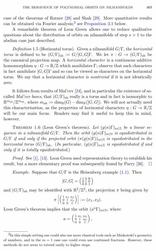
A remarkable theorem of Leon Green allows one to reduce qualitative
questions about the distribution of orbits on nilmanifolds of step s > 1 to the
abelian case just described.
Definition 1.5 (Horizontal torus). Given a nilmanifold G/Γ, the horizontal
torus is defined to be (G/Γ)ab := G/[G,G]Γ. We let π : G → (G/Γ)ab be
the canonical projection map. A horizontal character is a continuous additive
homomorphism η : G→ R/Z which annihilates Γ; observe that such characters
in fact annihilate [G,G]Γ and so can be viewed as characters on the horizontal
torus. We say that a horizontal character is nontrivial if it is not identically
zero.
It follows from results of Mal’cev [24], and in particular the existence of so-
called Mal’cev bases, that (G/Γ)ab really is a torus and in fact is isomorphic to
Rmab/Zmab , where mab := dimR(G)− dimR([G,G]). We will not actually need
this characterisation, as the properties of horizontal characters η : G → R/Zwill be our main focus. Readers may find it useful to keep this in mind,
however.
Theorem 1.6 (Leon Green’s theorem). Let (g(n)Γ)n∈Z be a linear se-
quence in a nilmanifold G/Γ. Then the orbit (g(n)Γ)n∈N is equidistributed in
G/Γ if and only if the projected orbit (π(g(n)Γ))n∈N is equidistributed in the
horizontal torus (G/Γ)ab. (In particular, (g(n)Γ)n∈Z is equidistributed if and
only if it is totally equidistributed.)
Proof. See [1], [13]. Leon Green used representation theory to establish his
result, but a more elementary proof was subsequently found by Parry [26].
Example. Suppose that G/Γ is the Heisenberg example (1.1). Then
[G,G] =(
1 0 R0 1 00 0 1
)and (G/Γ)ab may be identified with R2/Z2, the projection π being given by
π
ïÅ1 x1 x20 1 x30 0 1
ãò:= (x1, x3).
Leon Green’s theorem implies that the orbit (anΓ)n∈N, where
a =
Å1 α1 α20 1 α30 0 1
ã,
2In this simple setting one could also use more classical tools such as Minkowski’s geometry
of numbers, and in the m = 1 case one could even use continued fractions. However, these
methods do not seem to extend easily to higher steps.

470 BEN GREEN and TERENCE TAO
is equidistributed in G/Γ if and only if 1, α1, and α3 are independent over Q.
It is already somewhat nontrivial to establish this result directly.
By Kronecker’s theorem, we can then recast Theorem 1.6 in the following
equivalent formulation.
Theorem 1.7 (Leon Green’s theorem, again). Let (g(n)Γ)n∈Z be a linear
sequence in a nilmanifold G/Γ. Then exactly one of the following statements
is true:
(i) (g(n)Γ)n∈N is equidistributed in G/Γ.
(ii) There exists a nontrivial horizontal character η : G → R/Z such that
η g is constant.
Qualitative equidistribution theory of polynomial sequences. While our pri-
mary applications are concerned with linear sequences, it turns out for various
technical reasons that it is important to work in the more general class of
polynomial sequences.
Definition 1.8 (Polynomial sequences in nilpotent groups). Suppose that
G is a nilpotent group with a filtration G•. Let g : Z → G be a sequence. If
h ∈ Z, we write ∂hg := g(n+h)g(n)−1. We say that g is a polynomial sequence
with coefficients in G•, and write g ∈ poly(Z, G•), if ∂hi . . . ∂h1g takes values
in Gi for all positive integers i and for all choices of h1, . . . , hi ∈ Z. In this
case we say that g has degree d. If g lies in poly(G•) for some filtration G•,
then we simply say that g is a polynomial sequence.
This definition is a little abstract. However we will show in Section 6 that
g : Z → G is a polynomial sequence if and only if g has the form g(n) =
ap1(n)1 . . . a
pk(n)k , where a1, . . . , ak ∈ G and the pi : N → N are polynomials. In
particular, a linear sequence g(n) = anx is a polynomial sequence, and in fact
since ∂h1g(n) = ah1 and ∂h2∂h1g(n) = idG, it is clear that such a sequence has
coefficients in the lower central series filtration G•. Note carefully that the
degree of a linear sequence is equal to the step s of the underlying Lie group
G and is not equal to one as the name “linear” might suggest.
A remarkable result of Lazard and Leibman [18], [19], [20] asserts that
poly(Z, G•) is a group. We will prove this in Section 6, and it will play a key
role in several of our arguments.
Theorem 1.6 was extended by Liebman [22] to the case when g(n) is a
polynomial sequence rather than a linear one. In particular, he showed the
following generalisation of Theorem 1.7.
Theorem 1.9 (Leibman’s theorem [22]). Suppose that G/Γ is a nilman-
ifold and that g : Z → G is a polynomial sequence. Then exactly one of the
following statements is true:

THE BEHAVIOUR OF POLYNOMIAL ORBITS ON NILMANIFOLDS 471
(i) (g(n)Γ)n∈N is equidistributed in G/Γ.
(ii) There exists a nontrivial horizontal character η : G → R/Z such that
η g is constant.
Remark. This theorem significantly generalises the classical theorem of
Weyl that a polynomial sequence in R/Z is equidistributed unless all of its
nonconstant coefficients are rational. We will in fact use a quantitative version
of Weyl’s theorem in our arguments; see Proposition 4.3 below.
We can iterate this theorem to establish a factorisation result. We first
need some notation.
Definition 1.10 (Rational subgroup). LetG/Γ be a nilmanifold. A rational
subgroup of G is a closed connected subgroup G′ of G such that G′Γ/Γ ∼=G′/Γ′ = G′/(G′ ∩ Γ) is a closed submanifold of G/Γ (or equivalently, that Γ′
is a cocompact subgroup of G′). We say that G′ is proper if G′ 6= G.
Example. If G/Γ is a nilmanifold (that is to say if there exists a uniform
subgroup Γ 6 G), one can show that each member Gi of the lower central
series is a rational subgroup; see, e.g., [4] or [24].
Definition 1.11 (Rational sequence). Let G/Γ be a nilmanifold. A rational
group element is any g ∈ G such that gr ∈ Γ for some integer r > 0. A rational
point is any point in G/Γ of the form gΓ for some rational group element g.
A sequence (g(n)Γ)n∈Z is rational if every element g(n)Γ in the sequence is a
rational point.
Remark. It is not difficult to show that the rational group elements form
a dense subgroup of G that contains Γ; see Lemma A.11. We will show in
Lemma A.12 that any polynomial sequence in G/Γ which is rational is auto-
matically periodic.
Corollary 1.12 (Factorisation theorem for polynomial sequences). Let
(g(n)Γ)n∈Z be a polynomial sequence in a nilmanifold G/Γ. Then there exists
a rational subgroup G′ of G and a factorisation g = εg′γ, where ε ∈ G is
a constant, g′ : Z → G′ is a polynomial sequence such that (g′(n)Γ′)n∈N is
totally equidistributed in G′/Γ′ (where Γ′ := G ∩ Γ), and γ : Z → G is a
polynomial sequence such that the sequence (γ(n)Γ)n∈N is rational (and hence,
by Lemma A.12(i), is periodic).
Proof. We give a sketch of this argument only; we will repeat this argu-
ment in more detail when proving Theorem 1.19 below.
We induct on the dimension m of G/Γ, assuming that the claim has al-
ready been proven for all nilmanifolds of lesser dimension. By replacing g(n)
with g(0)−1g(n) if necessary (absorbing the g(0) factor into the ε term), we
may normalise so that g(0) = idG. If (g(n)Γ)n∈Z is equidistributed on G/Γ,

472 BEN GREEN and TERENCE TAO
then it is totally equidistributed by Leibman’s theorem, and we are done (with
g′ = g, G′ = G, and ε, γ trivial). So we may assume that (g(n)Γ)n∈Z is not
equidistributed. By Leibman’s theorem, there exists a nontrivial horizontal
character η : G → R/Z such that η g is constant. In fact, by our normali-
sation g(0) = idG, we must have η g ≡ 0, thus g takes values in ker(η). It
is then not difficult to factorise g = g0γ0, where γ0 is a polynomial sequence
with (γ0(n)Γ)n∈Z rational and periodic, and g0 is a polynomial sequence taking
values in the proper rational subgroup G′ 6 G, defined to be the connected
component of ker(η) which contains the origin. The claim then follows by
applying the induction hypothesis to the sequence (g0(n)Γ′)n∈Z in the nilman-
ifold G′/Γ′, which has dimension m− 1, and using the fact that the product of
two rational group elements is again rational, as well as the trivial observation
that rational group elements of G′ are automatically rational group elements
of G also.
Remark. In words, this corollary asserts that in the qualitative setting,
one can decompose
(arbitrary polynomial sequence)
= (constant)× (totally equidistributed)× (periodic).
An inspection of the proof reveals that one can in fact take the constant ε to
be g(0).
As a corollary, we obtain a Ratner-Shah type theorem for polynomial
sequences in nilmanifolds, first established by Leibman [22].
Corollary 1.13 (Leibman’s Ratner-Shah type theorem for nilmanifolds).
Let (g(n)Γ)n∈Z be a polynomial sequence in a nilmanifold G/Γ. Then there ex-
ists a rational subgroup G′ of G, a group element ε ∈ G, and a rational periodic
sequence (xn)n∈Z in G/Γ with some period q such that for every r ∈ Z, the
sequence (g(qn+ r)Γ)n∈Z is totally equidistributed in εG′xr.
Remark. Shah [29] obtained a similar result for arbitrary discrete unipo-
tent (but linear) flows on a finite volume homogeneous space; the case of con-
tinuous unipotent linear flows was treated earlier by Ratner [28] (see [25] for
further discussion). Leibman’s proof of Corollary 1.13 does not use these re-
sults, but instead proceeds in two stages. Firstly, by iterating Theorem 1.6 (or
more precisely a generalisation of this theorem to the case when G is not nec-
essarily connected), a version of Corollary 1.13 for linear sequences is obtained.
Secondly, by utilising a lifting trick of Furstenberg [6, p. 31], the polynomial
case is deduced from the linear case. As we shall discuss shortly, these argu-
ments do not work well in the quantitative case, and one must instead grapple
with polynomial sequences directly.
THE BEHAVIOUR OF POLYNOMIAL ORBITS ON NILMANIFOLDS 473
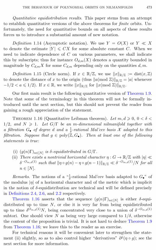
Quantitative equidistribution results. This paper stems from an attempt
to establish quantitative versions of the above theorems for finite orbits. Un-
fortunately, the need for quantitative bounds on all aspects of these results
forces us to introduce a substantial amount of new notation.
Definition 1.14 (Asymptotic notation). We use Y = O(X) or Y X
to denote the estimate |Y | 6 CX for some absolute constant C. When we
need to indicate dependence of C on various parameters, we shall indicate
this by subscripts; thus for instance Od,m(X) denotes a quantity bounded in
magnitude by Cd,mX for some Cd,m depending only on the quantities d,m.
Definition 1.15 (Circle norm). If x ∈ R/Z, we use ‖x‖R/Z := dist(x,Z)
to denote the distance of x to the origin (thus ‖a(mod Z)‖R/Z = |a| whenever
−1/2 < a 6 1/2). If x ∈ R, we write ‖x‖R/Z for ‖x(mod Z)‖R/Z.
Our first main result is the following quantitative version of Theorem 1.9.
Note that some of the terminology in this theorem will not be formally in-
troduced until the next section, but this should not prevent the reader from
gaining a rough appreciation of the statement.
Theorem 1.16 (Quantitative Leibman theorem). Let m, d > 0, 0 < δ <
1/2, and N > 1. Let G/Γ be an m-dimensional nilmanifold together with
a filtration G• of degree d and a 1δ -rational Mal’cev basis X adapted to this
filtration. Suppose that g ∈ poly(Z, G•). Then at least one of the following
statements is true:
(i) (g(n)Γ)n∈[N ] is δ-equidistributed in G/Γ.
(ii) There exists a nontrivial horizontal character η : G→ R/Z with |η| δ−Om,d(1) such that ‖η g(n)− η g(n− 1)‖R/Z δ−Om,d(1)/N for all
n ∈ [N ].
Remarks. The notions of a “1δ -rational Mal’cev basis adapted to G•” of
the modulus |η| of a horizontal character and of the metric which is implicit
in the notion of δ-equidistribution are technical and will be defined precisely
in Definitions 2.4, 2.6, and 2.2 respectively.
Theorem 1.16 asserts that the sequence (g(n)Γ)n∈[N ] is either δ-equi-
distributed up to time N , or else it is very far from being equidistributed
up to time δOm,d(1)N , being concentrated very close to a union of δ−Om,d(1)
subtori. One should view N as being very large compared to 1/δ, otherwise
the content of the proposition is trivial. It is not hard to deduce Theorem 1.9
from Theorem 1.16; we leave this to the reader as an exercise.
For technical reasons it will be convenient later to strengthen the state-
ment (ii) slightly, so as to also control higher “derivatives” ∂j(η g); see the
next section for more information.
474 BEN GREEN and TERENCE TAO
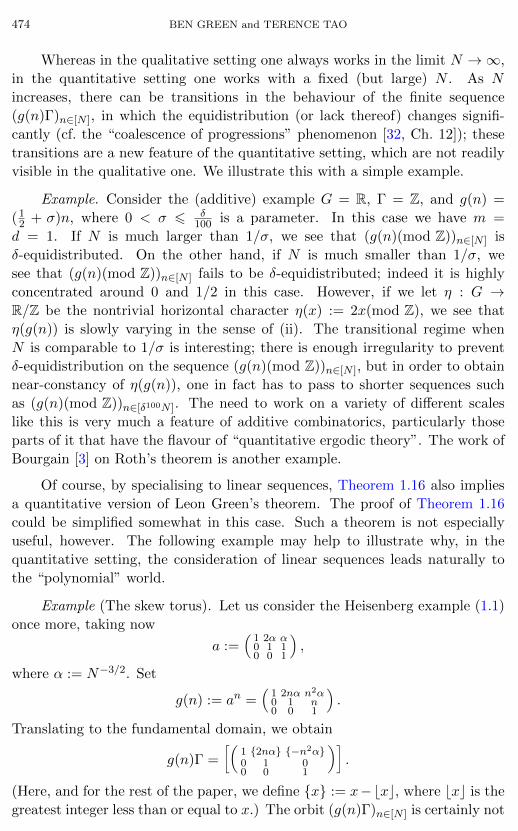
Whereas in the qualitative setting one always works in the limit N →∞,
in the quantitative setting one works with a fixed (but large) N . As N
increases, there can be transitions in the behaviour of the finite sequence
(g(n)Γ)n∈[N ], in which the equidistribution (or lack thereof) changes signifi-
cantly (cf. the “coalescence of progressions” phenomenon [32, Ch. 12]); these
transitions are a new feature of the quantitative setting, which are not readily
visible in the qualitative one. We illustrate this with a simple example.
Example. Consider the (additive) example G = R, Γ = Z, and g(n) =
(12 + σ)n, where 0 < σ 6 δ
100 is a parameter. In this case we have m =
d = 1. If N is much larger than 1/σ, we see that (g(n)(mod Z))n∈[N ] is
δ-equidistributed. On the other hand, if N is much smaller than 1/σ, we
see that (g(n)(mod Z))n∈[N ] fails to be δ-equidistributed; indeed it is highly
concentrated around 0 and 1/2 in this case. However, if we let η : G →R/Z be the nontrivial horizontal character η(x) := 2x(mod Z), we see that
η(g(n)) is slowly varying in the sense of (ii). The transitional regime when
N is comparable to 1/σ is interesting; there is enough irregularity to prevent
δ-equidistribution on the sequence (g(n)(mod Z))n∈[N ], but in order to obtain
near-constancy of η(g(n)), one in fact has to pass to shorter sequences such
as (g(n)(mod Z))n∈[δ100N ]. The need to work on a variety of different scales
like this is very much a feature of additive combinatorics, particularly those
parts of it that have the flavour of “quantitative ergodic theory”. The work of
Bourgain [3] on Roth’s theorem is another example.
Of course, by specialising to linear sequences, Theorem 1.16 also implies
a quantitative version of Leon Green’s theorem. The proof of Theorem 1.16
could be simplified somewhat in this case. Such a theorem is not especially
useful, however. The following example may help to illustrate why, in the
quantitative setting, the consideration of linear sequences leads naturally to
the “polynomial” world.
Example (The skew torus). Let us consider the Heisenberg example (1.1)
once more, taking now
a :=(
1 2α α0 1 10 0 1
),
where α := N−3/2. Set
g(n) := an =(
1 2nα n2α0 1 n0 0 1
).
Translating to the fundamental domain, we obtain
g(n)Γ =
ïÅ1 2nα −n2α0 1 00 0 1
ãò.
(Here, and for the rest of the paper, we define x := x−bxc, where bxc is the
greatest integer less than or equal to x.) The orbit (g(n)Γ)n∈[N ] is certainly not
THE BEHAVIOUR OF POLYNOMIAL ORBITS ON NILMANIFOLDS 475
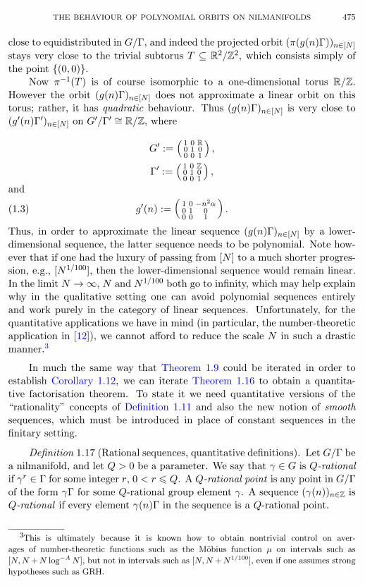
close to equidistributed in G/Γ, and indeed the projected orbit (π(g(n)Γ))n∈[N ]
stays very close to the trivial subtorus T ⊆ R2/Z2, which consists simply of
the point (0, 0).Now π−1(T ) is of course isomorphic to a one-dimensional torus R/Z.
However the orbit (g(n)Γ)n∈[N ] does not approximate a linear orbit on this
torus; rather, it has quadratic behaviour. Thus (g(n)Γ)n∈[N ] is very close to
(g′(n)Γ′)n∈[N ] on G′/Γ′ ∼= R/Z, where
G′ :=(
1 0 R0 1 00 0 1
),
Γ′ :=(
1 0 Z0 1 00 0 1
),
and
(1.3) g′(n) :=
Å1 0 −n2α0 1 00 0 1
ã.
Thus, in order to approximate the linear sequence (g(n)Γ)n∈[N ] by a lower-
dimensional sequence, the latter sequence needs to be polynomial. Note how-
ever that if one had the luxury of passing from [N ] to a much shorter progres-
sion, e.g., [N1/100], then the lower-dimensional sequence would remain linear.
In the limit N →∞, N and N1/100 both go to infinity, which may help explain
why in the qualitative setting one can avoid polynomial sequences entirely
and work purely in the category of linear sequences. Unfortunately, for the
quantitative applications we have in mind (in particular, the number-theoretic
application in [12]), we cannot afford to reduce the scale N in such a drastic
manner.3
In much the same way that Theorem 1.9 could be iterated in order to
establish Corollary 1.12, we can iterate Theorem 1.16 to obtain a quantita-
tive factorisation theorem. To state it we need quantitative versions of the
“rationality” concepts of Definition 1.11 and also the new notion of smooth
sequences, which must be introduced in place of constant sequences in the
finitary setting.
Definition 1.17 (Rational sequences, quantitative definitions). Let G/Γ be
a nilmanifold, and let Q > 0 be a parameter. We say that γ ∈ G is Q-rational
if γr ∈ Γ for some integer r, 0 < r 6 Q. A Q-rational point is any point in G/Γ
of the form γΓ for some Q-rational group element γ. A sequence (γ(n))n∈Z is
Q-rational if every element γ(n)Γ in the sequence is a Q-rational point.
3This is ultimately because it is known how to obtain nontrivial control on aver-
ages of number-theoretic functions such as the Mobius function µ on intervals such as
[N,N +N log−AN ], but not in intervals such as [N,N +N1/100], even if one assumes strong
hypotheses such as GRH.

476 BEN GREEN and TERENCE TAO
Definition 1.18 (Smooth sequences). Let G/Γ be a nilmanifold with a
Mal’cev basis X . Let (ε(n))n∈Z be a sequence in G, and let M,N > 1. We
say that (ε(n))n∈Z is (M,N)-smooth if we have d(ε(n), idG) 6 M and d(ε(n),
ε(n−1)) 6M/N for all n ∈ [N ], where the metric d = dX on G will be defined
in Definition 2.2.
Note that the notion of a (M,N)-smooth sequence collapses to that of a
constant sequence in the limit N →∞ (holding M fixed).
Theorem 1.19 (Factorisation theorem). Let m, d > 0, and let M0, N > 1
and A > 0 be real numbers. Suppose that G/Γ is an m-dimensional nilmanifold
together with a filtration G• of degree d. Suppose that X is an M0-rational
Mal’cev basis X adapted to G• and that g ∈ poly(Z, G•). Then there is an
integer M with M0 6M MOA,m,d(1)0 , a rational subgroup G′ ⊆ G, a Mal’cev
basis X ′ for G′/Γ′ in which each element is an M -rational combination of
the elements of X , and a decomposition g = εg′γ into polynomial sequences
ε, g′, γ ∈ poly(Z, G•) with the following properties :
(i) ε : Z→ G is (M,N)-smooth ;
(ii) g′ : Z→ G′ takes values in G′, and the finite sequence (g′(n)Γ′)n∈[N ] is
totally 1/MA-equidistributed in G′/Γ′, using the metric dX ′ on G′/Γ′;
(iii) γ : Z → G is M -rational, and (γ(n)Γ)n∈Z is periodic with period at
most M .
Remark. In words, this corollary asserts that in the quantitative setting,
one can decompose
(arbitrary polynomial sequence)
= (smooth)× (totally equidistributed)× (periodic).
The notion of a subgroup G′ being M -rational relative to a Mal’cev basis Xwill be defined in Definition 2.5. This result has some faint resemblance to
the Szemeredi regularity lemma [30], although with the key difference that our
bounds here are all polynomial in nature.
The derivation of Theorem 1.19 from Theorem 1.16 will be performed in
Section 8–10.
We will use Theorem 1.19 in [12] in order to establish the Mobius and
Nilsequences conjecture MN(s) from [11] for arbitrary step s. For this applica-
tion, it is important that all bounds here are only polynomial in M and that
the equidistribution is established on progressions of length linear in N (as
opposed to N c for some small c > 0).
Just as Corollary 1.12 implies a Ratner-type theorem, namely Corol-
lary 1.13, it is not hard to deduce the following result from Theorem 1.19.

THE BEHAVIOUR OF POLYNOMIAL ORBITS ON NILMANIFOLDS 477
Corollary 1.20 (Ratner-type theorem for polynomial nilsequences). Let
m, d > 0, 0 < δ < 1/2, and N > 1. Suppose that G/Γ is an m-dimensional nil-
manifold, that G• is a filtration of degree d on G, and that X is a 1/δ-rational
Mal’cev basis adapted to G•. Suppose that g ∈ poly(Z, G•). Then we may
decompose [N ] as a union P1 ∪ · · · ∪ Pk of arithmetic progressions with length
δOm,d(1)N and the same common difference q, 1 6 q δ−Om,d(1), such that
each orbit (g(n)Γ)n∈Pi lies within δ (using the metric dX ) of xiG′yiΓ/Γ ⊆ G/Γ,
where xi ∈ G, yi ∈ G is δ−Om,d(1)-rational, and G′ is a closed subgroup of G
which is δ−Om,d(1)-rational relative to X . (This notion will be defined in the
next section.)
Remark. The reader may wish to compare this with [5], another recent
result on quantitative variants of Ratner’s theorem.
Let us conclude this introduction by remarking that our main theorem
actually applies to multiparameter polynomial mappings g : Zt → G. In the
infinitary setting such a generalisation was obtained by Leibman [21], and his
result has subsequently been applied in such papers as [2] and [23]. We have
taken the trouble to derive multiparameter extensions of our main results with
analogous finitary applications in mind; see Theorems 8.6 and 10.2.
2. Precise statements of results
In this section we define various “quantitative” concepts (such asQ-rational
Mal’cev bases, subgroups which are Q-rational relative to such a basis, and the
metrics dX and dG/Γ) which were needed to properly state the main results
from the introduction section. We also give a more precise version of Theo-
rem 1.16, which we will then spend the next several sections proving.
Mal’cev bases and metrics on G/Γ. The notion of Mal’cev coordinates
play a vital role in the quantitative theory of nilmanifolds. They allow us to
put a metric on G/Γ, which in turn allows us to define the notion of equidis-
tribution; they also quantify the “rationality” of various objects associated to
the nilmanifold. Mal’cev coordinates were introduced in [24], which contains a
nice discussion; they are covered quite extensively in the book [4], particularly
Chapters 1 and 5. We will also need several more quantitative statements
about Mal’cev coordinates, which we have placed in Appendix A. We recom-
mend that the reader dip into that appendix as and when required.
We will make use of the Lie algebra g of G together with the exponential
map exp : g → G. When G is a connected, simply-connected nilpotent Lie
group, the exponential map is a diffeomorphism; see [4, Th. 1.2.1]. In partic-
ular, we have a logarithm map log : G→ g. One does not really need to have
an understanding of the exponential and logarithm maps beyond some of their
formal properties, which we will list as we need them, in order to understand
this paper.
478 BEN GREEN and TERENCE TAO
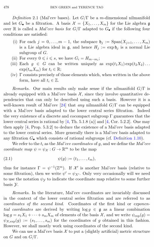
Definition 2.1 (Mal’cev bases). Let G/Γ be a m-dimensional nilmanifold
and let G• be a filtration. A basis X = X1, . . . , Xm for the Lie algebra g
over R is called a Mal’cev basis for G/Γ adapted to G• if the following four
conditions are satisfied:
(i) For each j = 0, . . . ,m − 1, the subspace hj := Span(Xj+1, . . . , Xm)
is a Lie algebra ideal in g, and hence Hj := exp hj is a normal Lie
subgroup of G.
(ii) For every 0 6 i 6 s, we have Gi = Hm−mi ;
(iii) Each g ∈ G can be written uniquely as exp(t1X1) exp(t2X2) . . .
exp(tmXm) for ti ∈ R;
(iv) Γ consists precisely of those elements which, when written in the above
form, have all ti ∈ Z.
Remarks. Our main results only make sense if the nilmanifold G/Γ is
already equipped with a Mal’cev basis X , since they involve quantitative de-
pendencies that can only be described using such a basis. However it is a
well-known result of Mal’cev [24] that any nilmanifold G/Γ can be equipped
with a Mal’cev basis adapted to the lower central series filtration. Indeed
the very existence of a discrete and cocompact subgroup Γ guarantees that the
lower central series is rational by [4, Th. 5.1.8 (a)] and [4, Cor. 5.2.2]. One may
then apply [4, Prop. 5.3.2] to deduce the existence of a Mal’cev basis adapted
to the lower central series. More generally there is a Mal’cev basis adapted to
any filtration G• which consists of rational subgroups (cf. Definition 1.10).
We refer to the ti as the Mal’cev coordinates of g, and we define the Mal’cev
coordinate map ψ = ψX : G→ Rm to be the map
(2.1) ψ(g) := (t1, . . . , tm),
thus for instance Γ = ψ−1(Zm). If X ′ is another Mal’cev basis (relative to
some filtration), then we write ψ′ = ψX′ . Only very occasionally will we need
to use the notation ψY to indicate the coordinate map relative to some further
basis Y.
Remarks. In the literature, Mal’cev coordinates are invariably discussed
in the context of the lower central series filtration and are referred to as
coordinates of the second kind. Coordinates of the first kind or exponen-
tial coordinates are derived by writing log g ∈ g as a linear combination
log g = s1X1 + · · ·+ smXm of elements of the basis X , and we write ψexp(g) =
ψX ,exp(g) := (s1, . . . , sm) for the coordinates of g obtained in this fashion.
However, we shall mostly work using coordinates of the second kind.
We can use a Mal’cev basis X to put a (slightly artificial) metric structure
on G and on G/Γ.

THE BEHAVIOUR OF POLYNOMIAL ORBITS ON NILMANIFOLDS 479
Definition 2.2 (Metrics on G and G/Γ). Let G/Γ be a nilmanifold with
Mal’cev basis X . We define d = dX : G × G → R>0 to be the largest metric
such that d(x, y) 6 |ψ(xy−1)| for all x, y ∈ G, where | · | denotes the `∞-norm
on Rm. More explicitly, we have
d(x, y)=inf
n−1∑i=0
min(|ψ(xi−1x−1i )|, |ψ(xix
−1i−1)|) :x0, . . . , xn ∈G;x0 =x;xn= y
.
This descends to a metric on G/Γ by setting
d(xΓ, yΓ) := infd(x′, y′) : x′, y′ ∈ G;x′ ≡ x(mod Γ); y′ ≡ y(mod Γ).It turns out that this is indeed4 a metric on G/Γ; this essentially follows from
the discreteness of Γ in G, and we will prove it in Lemma A.15. Since d is
right-invariant, we also have
d(xΓ, yΓ) = infγ∈Γ
d(x, yγ).
When the letter d is used for a metric, it will always denote the metric dXrelative to some basis X that is already under discussion. The symbol d′ will
be used for the metric defined using some other basis X ′. On the very rare
occasions (for example in the proof of Lemma 7.4) where the metric relative to
some further basis is under consideration, we will indicate this explicitly using
subscripts.
Quantitative rationality. Now we define the concept of rational nilmani-
folds and subgroups.
Definition 2.3 (Height). The height of a real number x is defined as
max(|a|, |b|) if x = a/b is rational in reduced form and ∞ if x is irrational.
Definition 2.4 (Rationality of a basis). Let G/Γ be a nilmanifold, and let
Q > 0. We say that a Mal’cev basis X for G/Γ is Q-rational if all of the
structure constants cijk in the relations
[Xi, Xj ] =∑k
cijkXk
are rational with height at most Q.
Definition 2.5 (Rational subgroups). Suppose that a nilmanifold G/Γ is
given together with a Mal’cev basis X = X1, . . . , Xm and that Q > 0.
4We note that this metric structure is a little more specific than in some of our previous
papers, notably in [11, §8]. This will not cause any difficulty, as the metrics in that paper are
equivalent to the one given here, up to constants depending on G,Γ, and X . Indeed, at small
scales, d agrees with the distance function given by the unique right-invariant Riemannian
metric on G whose value at the origin is equal to that of the Euclidean metric at the origin
of Rm, pulled back by ψ; see also Lemma A.4.

480 BEN GREEN and TERENCE TAO
Suppose that G′ ⊆ G is a closed connected subgroup. We say that G′ is
Q-rational relative to X if the Lie algebra g′ has a basis X ′ = X ′1, . . . , X ′m′consisting of linear combinations
∑mi=1 aiXi, where ai are rational numbers
with height at most Q for all i.
Definition 2.6 (Modulus of a horizontal character). Suppose that G/Γ is a
nilmanifold with a Mal’cev basis X . Suppose that η : G→ R/Z is a horizontal
character, that is to say a homomorphism from G to R/Z which annihilates Γ.
Then, when written in coordinates relative to X , properties (iii) and (iv) of
Proposition 2.1 imply that η(g) = k · ψ(g) for some unique k ∈ Zm. We write
|η| := |k|.
Smooth polynomial sequences. For technical reasons it will be convenient
to quantify the smoothness of sequences, such as the sequence ε(n) appearing
in Theorem 1.19, in a slightly different manner from that used so far.
Definition 2.7 (Smoothness norms). Suppose that g : Z→ R/Z is a poly-
nomial sequence of degree d. Then g may be written uniquely as
g(n) = α0 + α1
Çn
1
å+ · · ·+ αd
Çn
d
å,
where αi is in fact equal to ∂ig(0). For any N > 0, we define the smoothness
norm
‖g‖C∞[N ] := sup16j6d
N j‖αj‖R/Z.
The smoothness norm ‖ · ‖C∞[N ] is designed to capture the notion of a
polynomial sequence which is slowly-varying. Indeed, the following lemma is
easily verified.
Lemma 2.8 (Smooth polynomials vary slowly). Let g : Z → R/Z be a
polynomial sequence of degree d, and let N > 0. Then for any n ∈ [N ], we have
‖g(n)− g(n− 1)‖R/Z d1
N‖g‖C∞[N ].
In view of this lemma, we see that Theorem 1.16 will be an immediate
consequence of the following more precise statement. This is in fact the main
technical result in our paper, and we will use it to derive all our other main
results.
Theorem 2.9 (Quantitative Leibman theorem). Let m, d > 0, 0 < δ <
1/2, and N > 1. Suppose that G/Γ is an m-dimensional nilmanifold together
with a filtration G• and that X is a 1δ -rational Mal’cev basis adapted to G•.
Suppose that g ∈ poly(Z, G•). If (g(n)Γ)n∈[N ] is not δ-equidistributed, then
there is a horizontal character η with 0 < |η| δ−Om,d(1) such that
‖η g‖C∞[N ] δ−Om,d(1).
THE BEHAVIOUR OF POLYNOMIAL ORBITS ON NILMANIFOLDS 481
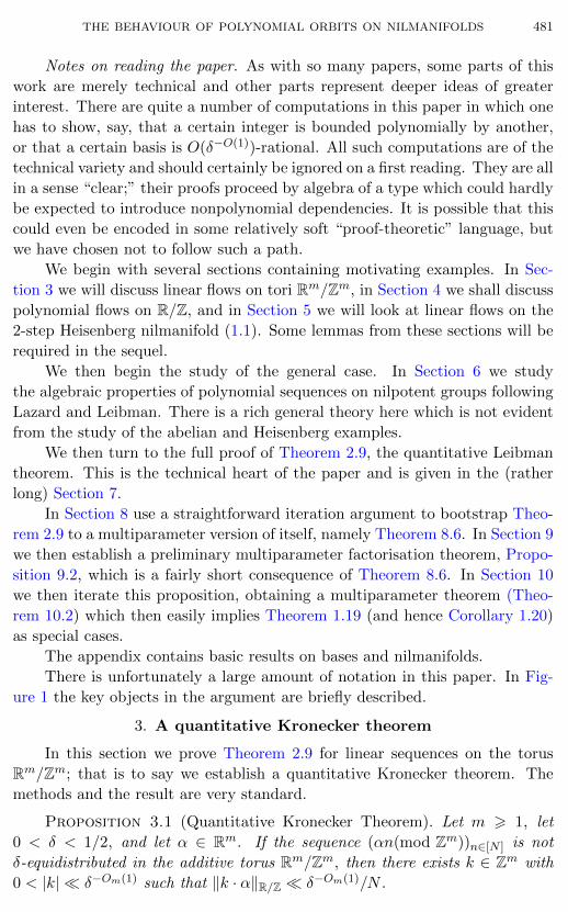
Notes on reading the paper. As with so many papers, some parts of this
work are merely technical and other parts represent deeper ideas of greater
interest. There are quite a number of computations in this paper in which one
has to show, say, that a certain integer is bounded polynomially by another,
or that a certain basis is O(δ−O(1))-rational. All such computations are of the
technical variety and should certainly be ignored on a first reading. They are all
in a sense “clear;” their proofs proceed by algebra of a type which could hardly
be expected to introduce nonpolynomial dependencies. It is possible that this
could even be encoded in some relatively soft “proof-theoretic” language, but
we have chosen not to follow such a path.
We begin with several sections containing motivating examples. In Sec-
tion 3 we will discuss linear flows on tori Rm/Zm, in Section 4 we shall discuss
polynomial flows on R/Z, and in Section 5 we will look at linear flows on the
2-step Heisenberg nilmanifold (1.1). Some lemmas from these sections will be
required in the sequel.
We then begin the study of the general case. In Section 6 we study
the algebraic properties of polynomial sequences on nilpotent groups following
Lazard and Leibman. There is a rich general theory here which is not evident
from the study of the abelian and Heisenberg examples.
We then turn to the full proof of Theorem 2.9, the quantitative Leibman
theorem. This is the technical heart of the paper and is given in the (rather
long) Section 7.
In Section 8 use a straightforward iteration argument to bootstrap Theo-
rem 2.9 to a multiparameter version of itself, namely Theorem 8.6. In Section 9
we then establish a preliminary multiparameter factorisation theorem, Propo-
sition 9.2, which is a fairly short consequence of Theorem 8.6. In Section 10
we then iterate this proposition, obtaining a multiparameter theorem (Theo-
rem 10.2) which then easily implies Theorem 1.19 (and hence Corollary 1.20)
as special cases.
The appendix contains basic results on bases and nilmanifolds.
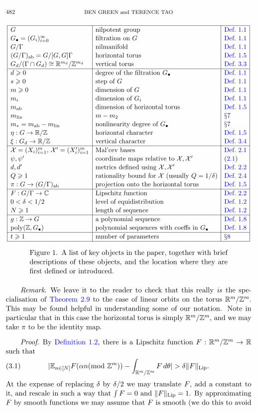
There is unfortunately a large amount of notation in this paper. In Fig-
ure 1 the key objects in the argument are briefly described.
3. A quantitative Kronecker theorem
In this section we prove Theorem 2.9 for linear sequences on the torus
Rm/Zm; that is to say we establish a quantitative Kronecker theorem. The
methods and the result are very standard.
Proposition 3.1 (Quantitative Kronecker Theorem). Let m > 1, let
0 < δ < 1/2, and let α ∈ Rm. If the sequence (αn(mod Zm))n∈[N ] is not
δ-equidistributed in the additive torus Rm/Zm, then there exists k ∈ Zm with
0 < |k| δ−Om(1) such that ‖k · α‖R/Z δ−Om(1)/N .
482 BEN GREEN and TERENCE TAO
G nilpotent group Def. 1.1
G• = (Gi)∞i=0 filtration on G Def. 1.1
G/Γ nilmanifold Def. 1.1
(G/Γ)ab = G/[G,G]Γ horizontal torus Def. 1.5
Gd/(Γ ∩Gd) ∼= Rmd/Zmd vertical torus Def. 3.3
d > 0 degree of the filtration G• Def. 1.1
s > 0 step of G Def. 1.1
m > 0 dimension of G Def. 1.1
mi dimension of Gi Def. 1.1
mab dimension of horizontal torus Def. 1.5
mlin m−m2 §7m∗ = mab −mlin nonlinearity degree of G• §7η : G→ R/Z horizontal character Def. 1.5
ξ : Gd → R/Z vertical character Def. 3.4
X = (Xi)mi=1, X ′ = (X ′i)
mi=1 Mal’cev bases Def. 2.1
ψ,ψ′ coordinate maps relative to X ,X ′ (2.1)
d, d′ metrics defined using X ,X ′ Def. 2.2
Q > 1 rationality bound for X (usually Q = 1/δ) Def. 2.4
π : G→ (G/Γ)ab projection onto the horizontal torus Def. 1.5
F : G/Γ→ C Lipschitz function Def. 2.2
0 < δ < 1/2 level of equidistribution Def. 1.2
N > 1 length of sequence Def. 1.2
g : Z→ G a polynomial sequence Def. 1.8
poly(Z, G•) polynomial sequences with coeffs in G• Def. 1.8
t > 1 number of parameters §8
Figure 1. A list of key objects in the paper, together with brief
descriptions of these objects, and the location where they are
first defined or introduced.
Remark. We leave it to the reader to check that this really is the spe-
cialisation of Theorem 2.9 to the case of linear orbits on the torus Rm/Zm.
This may be found helpful in understanding some of our notation. Note in
particular that in this case the horizontal torus is simply Rm/Zm, and we may
take π to be the identity map.
Proof. By Definition 1.2, there is a Lipschitz function F : Rm/Zm → Rsuch that
(3.1) |En∈[N ]F (αn(mod Zm))−∫Rm/Zm
F dθ| > δ‖F‖Lip.
At the expense of replacing δ by δ/2 we may translate F , add a constant to
it, and rescale in such a way that∫F = 0 and ‖F‖Lip = 1. By approximating
F by smooth functions we may assume that F is smooth (we do this to avoid

THE BEHAVIOUR OF POLYNOMIAL ORBITS ON NILMANIFOLDS 483
any technical issues regarding convergence of Fourier series). We now use a
standard manœuvre to approximate F by a function which has finite support
in frequency space (cf. [10, Lemma A.9]).
Consider the Fejer kernel K : Rm/Zm → R+ defined by
K(θ) :=1
mes(Q)1Q ∗
1
mes(Q)1Q(θ),
where Q := [− δ16m ,
δ16m ]m ⊂ Rm/Zm is a small cube and ∗ denotes the usual
convolution operation on the torus Rm/Zm. It is immediate that K is a non-
negative function supported in Q with
(3.2)
∫Rm/Zm
K = 1.
A simple calculation also establishes the estimate
(3.3)∑
k∈Zm:|k|>M|K(k)| m δ−2mM−1
for all M > 1, where the Fourier coefficient is defined by
K(k) :=
∫Rm/Zm
K(θ)e(−θ · k) dθ
and e(x) := e2πix is the standard character on R/Z. We also have the crude
bound
(3.4) |“F (k)| 6 ‖F‖∞ 6 ‖F‖Lip 6 1
for all k ∈ Zm.
Set F1 := F ∗K. Since ‖F‖Lip = 1, and K is supported in Q and satisfies
(3.2), a standard computation shows that
‖F − F1‖∞ 6 δ/8.
Choose M := Cmδ−2m−1 for some suitably large Cm, and set
F2(θ) :=∑
k∈Zm:0<|k|6M
“F1(k)e(k · θ).
Noting that “F1(0) = 0, facts (3.3), (3.4), and the Fourier inversion formula
imply that
‖F1 − F2‖∞ 6 δ/8.It follows that ‖F − F2‖∞ 6 δ/4, which means, in view of the failure of (3.1),
that
|En∈[N ]F2(nαZm)| > δ/4.Applying (3.4) once more we see that there is some k, 0 < |k| 6M , such that
|En∈[N ]e(nk · α)| m δMm δOm(1).

484 BEN GREEN and TERENCE TAO
The result now follows immediately from the standard estimate
|En∈[N ]e(nt)| min
Ç1,
1
N‖t‖R/Z
å,
which follows from summing the geometric progression.
Let us now record a corollary of the m = 1 version of this result which
will be used several times in the sequel. This gives stronger information in the
case that (nα(mod Z))n∈[N ] is very far from being equidistributed.
Lemma 3.2 (Strongly recurrent linear functions are highly non-diophan-
tine). Let α ∈ R, 0 < δ < 1/2, and 0 < ε 6 δ/2, and let I ⊆ R/Z be an
interval of length ε such that αn ∈ I for at least δN values of n ∈ [N ]. Then
there is some k ∈ Z with 0 < |k| δ−O(1) such that ‖kα‖R/Z εδ−O(1)/N .
Proof. Taking F to be a Lipschitz approximation to the interval I, we see
immediately that our assumption precludes (αn(mod Z))n∈[N ] from being δ10-
equidistributed. It follows from the case m = 1 of Proposition 3.1 that there
is some k ∈ Z, |k| δ−C , such that ‖kα‖R/Z δ−C/N , where C = O(1).
Write β := ‖qα‖R/Z. Let n0 ∈ Z be arbitrary, and suppose that n′ ranges
over any interval of integers J of length at most 1/β. The number of n′ for
which α(n0 + qn′)Z ∈ I is then at most 1 + ε/β. Since [N ] may be divided into
6 2q + βN progressions of the form n0 + qn′ : n′ ∈ J, we obtain from our
assumption the inequality
(3.5) δN 6 #n ∈ [N ] : αnZ ∈ I 6 (1 +ε
β)(2q+ βN) q+
εq
β+ βN + εN.
Now the lemma is trivial if N δ−10C and follows immediately from Proposi-
tion 3.1 when ε δ10C , so suppose that neither of these is the case. Then all
of the terms except the second on the right-hand side of (3.5) are negligible,
and we deduce that
δN qε/β.
This immediately implies the result.
The main idea in the proof of Proposition 3.1, of course, was that the
space of Lipschitz functions is essentially spanned by the space of pure phase
functions e(k · θ). Thus we were able to assert that if the condition (3.1) fails
for some F , then it also fails (albeit with a smaller value of δ) for a pure phase
function with not-too-large frequency.
A similar observation turns out to be essential in the analysis of polynomial
sequences on general nilmanifolds G/Γ (cf. the proof of [22, Th. 2.17]). Though
we will not be discussing general sequences for quite a while, this does seem
to be an appropriate place to state and prove a lemma which generalises the
THE BEHAVIOUR OF POLYNOMIAL ORBITS ON NILMANIFOLDS 485
observations just made. For this, we will be working primarily on the vertical
torus.
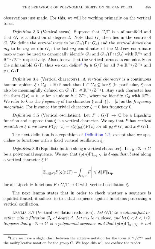
Definition 3.3 (Vertical torus). Suppose that G/Γ is a nilmanifold and
that G• is a filtration of degree d. Note that Gd then lies in the centre of
G. We define the vertical torus to be Gd/(Γ ∩Gd) and the vertical dimension
md to be md := dimGd; the last md coordinates of the Mal’cev coordinate
map ψ may be used to canonically identify Gd and Gd/(Γ∩Gd) with Rmd and
Rmd/Zmd respectively. Also observe that the vertical torus acts canonically on
the nilmanifold G/Γ, thus we can define5 θy ∈ G/Γ for all θ ∈ Rmd/Zmd and
y ∈ G/Γ.
Definition 3.4 (Vertical characters). A vertical character is a continuous
homomorphism ξ : Gd → R/Z such that Γ ∩ Gd ⊆ ker ξ (in particular, ξ can
also be meaningfully defined on Gd/Γd ∼= Rmd/Zmd). Any such character has
the form ξ(x) = k · x for a unique k ∈ Zmd , where we identify Gd with Rmd .
We refer to k as the frequency of the character ξ and |ξ| := |k| as the frequency
magnitude. For instance the trivial character ξ ≡ 0 has frequency 0.
Definition 3.5 (Vertical oscillation). Let F : G/Γ → C be a Lipschitz
function and suppose that ξ is a vertical character. We say that F has vertical
oscillation ξ if we have F (gd · x) = e(ξ(gd))F (x) for all gd ∈ Gd and x ∈ G/Γ.
The next definition is a repetition of Definition 1.2, except that we spe-
cialise to functions with a fixed vertical oscillation ξ.
Definition 3.6 (Equidistribution along a vertical character). Let g : Z→ G
be a polynomial sequence. We say that (g(n)Γ)n∈[N ] is δ-equidistributed along
a vertical character ξ if∣∣∣∣∣En∈[N ]F (g(n)Γ)−∫G/Γ
F
∣∣∣∣∣ 6 δ‖F‖Lip
for all Lipschitz functions F : G/Γ→ C with vertical oscillation ξ.
The next lemma states that in order to check whether a sequence is
equidistributed, it suffices to test that sequence against functions possessing a
vertical oscillation.
Lemma 3.7 (Vertical oscillation reduction). Let G/Γ be a nilmanifold to-
gether with a filtration G• of degree d. Let md be as above, and let 0 < δ < 1/2.
Suppose that g : Z→ G is a polynomial sequence and that (g(n)Γ)n∈[N ] is not
5Here we have a slight clash between the additive notation for the torus Rmd/Zmd and
the multiplicative notation for the group G. We hope this will not confuse the reader.

486 BEN GREEN and TERENCE TAO
δ-equidistributed. Then there is a vertical character ξ with |ξ| δ−Omd(1) such
that (g(n)Γ)n∈[N ] is not δOmd(1)-equidistributed along the vertical oscillation ξ.
Proof. We merely sketch this, for the argument is little more than a repeti-
tion of that used to prove Proposition 3.1. We begin with the same reductions.
That is, assuming the existence of an F : G/Γ→ C such that
(3.6)
∣∣∣∣∣En∈[N ]F (g(n)Γ)−∫G/Γ
F
∣∣∣∣∣ > δ‖F‖Lip,
we weaken δ to δ/2 and assume that∫G/Γ F = 0, that ‖F‖Lip = 1, and that F
is smooth.
Let K be the same Fejer-type kernel as before, and now take F1 : G→ Cto be the function obtained by convolving with K in each Gd/(Γ ∩ Gd) ∼=Rmd/Zmd-fibre; that is to say,
F1(y) :=
∫Rmd/Zmd
F (θy)K(θ)dθ.
Fourier expansion on Rmd/Zmd gives
F1(y) =∑
k∈Zmd
F∧(y; k)K(k),
where
F∧(y; k) :=
∫Rmd/Zmd
F (θy)e(−k · θ)dθ.
Now for gd ∈ Gd ∼= Rmd , we have
F∧(gdy; k) =
∫F ((θ + gd)y)e(−k · θ) dθ = e(k · gd)F∧(y; f);
thus each function F∧(y; k) has vertical oscillation ξ, where ξ(x) := k ·x is the
vertical character with frequency k.
Using exactly the same estimates as in the proof of Proposition 3.1, we
have ‖F − F2‖∞ 6 δ/4, where
F2(y) :=∑
k∈Zmd :|k|6QF∧(y; k)K(k)
for some Q = Cmdδ−2md−1. The rest of the argument proceeds exactly as
before, and we see that if we take F (y) := F∧(y; k) for suitable k ∈ Zmd ,
|k| δ−Omd(1), we have∣∣∣∣∣En∈[N ]F (g(n)Γ)−
∫G/Γ
F
∣∣∣∣∣ δOmd(1)‖F‖Lip.
Thus (g(n)Γ)n∈[N ] is not δOmd(1)-equidistributed along the vertical character
ξ, as desired.

THE BEHAVIOUR OF POLYNOMIAL ORBITS ON NILMANIFOLDS 487
4. The van der Corput trick and polynomial flows on tori
In the last section we introduced one important trick — the idea of decom-
posing a Lipschitz function into phases using Fourier analysis. In this section
we introduce a second trick - namely, the use of van der Corput’s inequality
— and use this trick to study polynomial sequences on tori Rm/Zm. Although
our language is somewhat different, this is really just a reprise of the standard
theory of Weyl sums as used, for instance, in the study of Waring’s problem
(see, for example, [33]).
Lemma 4.1 (van der Corput inequality). Let N,H be positive integers
and suppose that (an)n∈[N ] is a sequence of complex numbers. Extend (an) to
all of Z by defining an := 0 when n /∈ [N ]. Then
|En∈[N ]an|2 6N +H
HN
∑|h|6H
Ç1− |h|
H
åEn∈[N ]anan+h.
Proof. We have
∑n
an =1
H
∑−H<n6N
H−1∑h=0
an+h.
Thus, applying the Cauchy-Schwarz inequality, we have∣∣∣∑n
an∣∣∣2 =
1
H2
∣∣∣ ∑−H<n6N
H−1∑h=0
an+h
∣∣∣26N +H
H2
∑−H<n6N
∣∣∣H−1∑h=0
an+h
∣∣∣2=N +H
H2
∑−H<n6N
H−1∑h=0
H−1∑h′=0
an+han+h′ ,
which is equivalent to the right-hand side of the claimed inequality.
We will use the following simple (and rather crude) corollary of this, which
we phrase in the contrapositive.
Corollary 4.2 (van der Corput). Let N be a positive integer, and sup-
pose that (an)n∈[N ] is a sequence of complex numbers with |an| 6 1. Extend
(an) to all of Z by defining an := 0 when n /∈ [N ]. Suppose that 0 < δ < 1 and
that
|En∈[N ]an| > δ.
Then for at least δ2N/8 values of h ∈ [N ], we have
|En∈[N ]an+han| > δ2/8.

488 BEN GREEN and TERENCE TAO
Proof. The result is vacuous if N 6 4/δ2, so assume this is not the case.
Suppose for a contradiction that the result is false. Apply Lemma 4.1 with
H = N . Then it is easy to see that we have
δ2 6 |En∈[N ]an| 62
N
∑|h|6N
|En∈[N ]anan+h| 62
N
Ç1 + 2
Çδ2N
8+δ2N
8
åå,
where we have used the trivial estimate |En∈[N ]anan+h| 6 1 for those h ∈ [N ]
such that |En∈[N ]anan+h| > δ2/8, of which there are no more than δ2N/8.
Rearranging and using the fact that N > 4/δ2 we see that this is a contradic-
tion.
The next proposition is the main result of this section and is Theorem 2.9
in the case G = R, Γ = Z, and with g : Z→ G an arbitrary polynomial.
Proposition 4.3 (Weyl). Suppose that g : Z→R is a polynomial of de-
gree d, and let 0<δ<1/2. Then either (g(n)(mod Z))n∈[N ] is δ-equidistributed,
or else there is an integer k, 1 6 k δ−Od(1), such that ‖kg(mod Z)‖C∞[N ] δ−Od(1).
We will deduce this from the following, which is nothing but a reformula-
tion of Weyl’s exponential sum estimate (see, e.g., [33]).
Lemma 4.4 (Weyl’s exponential sum estimate). Suppose that g : Z → Ris a polynomial of degree d with leading coefficient αd and that
|En∈[N ]e(g(n))| > δ
for some 0 < δ < 1/2. Then there is k ∈ Z, |k| δ−Od(1), such that
‖kαd‖R/Z δ−Od(1)/Nd.
Proof. We proceed by induction on d, the result having been established
in Section 3 in the case d = 1. We may assume that N > δ−C′d for some large
C ′d since the result is trivial otherwise. Applying van der Corput’s estimate in
the form of Corollary 4.2, we deduce that there are δ2N values of h ∈ [N ]
such that
|En∈[N ]e(g(n+ h)− g(n))| δ2.
For each such h, g(n+h)− g(n) is a polynomial with degree d− 1 and leading
coefficient hdαd. Thus by the induction hypothesis there is, for δ2 values of
h ∈ [N ], some 1 6 qh δ−Od(1) such that we have
‖hqhdαd‖R/Z δ−Od(1)/Nd−1
for each of these values of h. Pigeonholing in the qh, this implies that there is
q, 1 6 q δ−Od(1), such that
‖hαd‖R/Z,δ−Od(1) δ−Od(1)/Nd−1
THE BEHAVIOUR OF POLYNOMIAL ORBITS ON NILMANIFOLDS 489
for δOd(1)N values of h ∈ [N ]. Since N is so large, Lemma 3.2 may applied
to conclude that there is q′ δ−Od(1) such that
‖qq′αd‖R/Z δ−Od(1)/Nd.
Redefining q := qq′, the result follows.
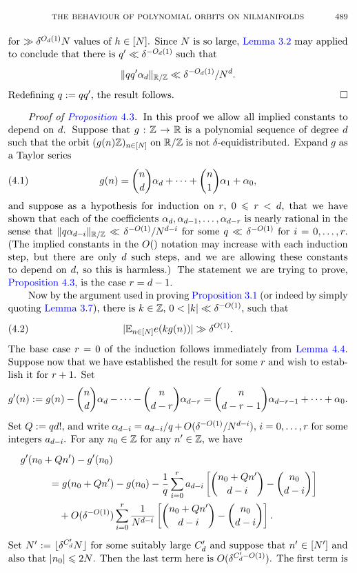
Proof of Proposition 4.3. In this proof we allow all implied constants to
depend on d. Suppose that g : Z → R is a polynomial sequence of degree d
such that the orbit (g(n)Z)n∈[N ] on R/Z is not δ-equidistributed. Expand g as
a Taylor series
(4.1) g(n) =
Çn
d
åαd + · · ·+
Çn
1
åα1 + α0,
and suppose as a hypothesis for induction on r, 0 6 r < d, that we have
shown that each of the coefficients αd, αd−1, . . . , αd−r is nearly rational in the
sense that ‖qαd−i‖R/Z δ−O(1)/Nd−i for some q δ−O(1) for i = 0, . . . , r.
(The implied constants in the O() notation may increase with each induction
step, but there are only d such steps, and we are allowing these constants
to depend on d, so this is harmless.) The statement we are trying to prove,
Proposition 4.3, is the case r = d− 1.
Now by the argument used in proving Proposition 3.1 (or indeed by simply
quoting Lemma 3.7), there is k ∈ Z, 0 < |k| δ−O(1), such that
(4.2) |En∈[N ]e(kg(n))| δO(1).
The base case r = 0 of the induction follows immediately from Lemma 4.4.
Suppose now that we have established the result for some r and wish to estab-
lish it for r + 1. Set
g′(n) := g(n)−Çn
d
åαd − · · · −
Çn
d− r
åαd−r =
Çn
d− r − 1
åαd−r−1 + · · ·+ α0.
Set Q := qd!, and write αd−i = ad−i/q+O(δ−O(1)/Nd−i), i = 0, . . . , r for some
integers ad−i. For any n0 ∈ Z for any n′ ∈ Z, we have
g′(n0 +Qn′)− g′(n0)
= g(n0 +Qn′)− g(n0)− 1
q
r∑i=0
ad−i
ñÇn0 +Qn′
d− i
å−Çn0
d− i
åô+O(δ−O(1))
r∑i=0
1
Nd−i
ñÇn0 +Qn′
d− i
å−Çn0
d− i
åô.
Set N ′ := bδC′dNc for some suitably large C ′d and suppose that n′ ∈ [N ′] and
also that |n0| 6 2N . Then the last term here is O(δC′d−O(1)). The first term is
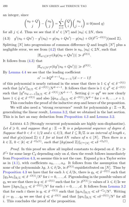
490 BEN GREEN and TERENCE TAO
an integer, sinceÇn0 +Q
j
å−Çn0
j
å=
j∑i=1
ÇQ
i
åÇn0
j − i
å≡ 0(mod q)
for all j 6 d. Thus we see that if n′ ∈ [N ′] and |n0| 6 2N , then
(4.3) g′(n0 +Qn′)− g′(n0) = g(n0 +Qn′)− g(n0) +O(δC′d−O(1))(mod Z).
Splitting [N ] into progressions of common difference Q and length [N ′] plus a
negligible error, we see from (4.2) that there is n0, |n0| 6 2N , such that
|En′∈[N ′]e(kg(n0 +Qn′))| δO(1).
It follows from (4.3) that
|En′∈[N ′]e(kg′(n0 +Qn′))| δO(1).
By Lemma 4.4 we see that the leading coefficient
α′ := kQd−r−1αd−r−1/(d− r − 1)!
of this polynomial is nearly rational in the sense that there is 1 6 q′ δ−O(1)
such that ‖q′α′‖R/Z δ−O(1)/Nd−r−1. It follows that there is 1 6 q′′ δ−O(1)
such that ‖q′′αd−r−1‖R/Z δ−O(1)/Nd−r−1. Setting q := qq′′ we now clearly
have 1 6 q δ−O(1) and also ‖qαd−i‖R/Z δ−O(1)/Nd−i for i = 0, . . . , r + 1.
This concludes the proof of the inductive step and hence of the proposition.
We will also need a “strong recurrence” result for polynomials g : Z→ R,
generalizing the linear result, Lemma 3.2, that we obtained in the last section.
This is in fact an easy deduction from Proposition 4.3 and Lemma 3.2.
Lemma 4.5 (Strongly recurrent polynomials are highly non-diophantine).
Let d > 0, and suppose that g : Z → R is a polynomial sequence of degree d.
Suppose that 0 < δ < 1/2 and ε 6 δ/2, that I ⊆ R/Z is an interval of length ε,
and that g(n)(mod Z) ∈ I for at least δN values of n ∈ [N ]. Then there is a
k ∈ Z, 0 < |k| δ−Od(1), such that ‖kg(mod Z)‖C∞[N ] εδ−Od(1).
Proof. In this proof we allow all implied constants to depend on d. If εδCd for some large Cd depending only on d, then the result follows immediately
from Proposition 4.3, so assume this is not the case. Expand g in a Taylor series
as in (4.1), with coefficients α0, . . . , αd. It follows from the assumption that
none of the polynomials λg, λ 6 δ/2ε, is δO(1)-equidistributed on [N ]. Thus by
Proposition 4.3 we have that for each λ 6 δ/2ε, there is qλ δ−O(1) such that
‖qλλαi‖R/Z δ−O(1)/N i for i = 0, . . . , d. Pigeonholing in the possible values of
qλ we see that there is q δ−O(1) such that for δO(1)/ε values of λ 6 δ/2ε we
have ‖λqαi‖R/Z δ−O(1)/N i for each i = 0, . . . , d. It follows from Lemma 3.2
that for each i there is qi δ−O(1) such that ‖qiαi‖R/Z εδ−Cd/N i. Writing
q := q1 . . . qd we see that q δ−O(1) and that ‖qαi‖R/Z εδ−O(1)/N i for all
i. This concludes the proof of the proposition.
THE BEHAVIOUR OF POLYNOMIAL ORBITS ON NILMANIFOLDS 491
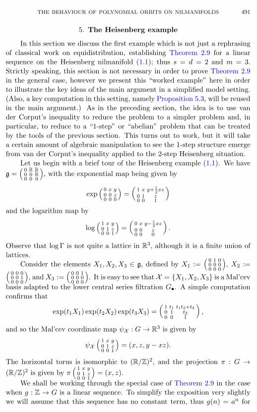
5. The Heisenberg example
In this section we discuss the first example which is not just a rephrasing
of classical work on equidistribution, establishing Theorem 2.9 for a linear
sequence on the Heisenberg nilmanifold (1.1); thus s = d = 2 and m = 3.
Strictly speaking, this section is not necessary in order to prove Theorem 2.9
in the general case, however we present this “worked example” here in order
to illustrate the key ideas of the main argument in a simplified model setting.
(Also, a key computation in this setting, namely Proposition 5.3, will be reused
in the main argument.) As in the preceding section, the idea is to use van
der Corput’s inequality to reduce the problem to a simpler problem and, in
particular, to reduce to a “1-step” or “abelian” problem that can be treated
by the tools of the previous section. This turns out to work, but it will take
a certain amount of algebraic manipulation to see the 1-step structure emerge
from van der Corput’s inequality applied to the 2-step Heisenberg situation.
Let us begin with a brief tour of the Heisenberg example (1.1). We have
g =(
0 R R0 0 R0 0 0
), with the exponential map being given by
exp( 0 x y
0 0 z0 0 0
)=
Å1 x y+ 1
2xz
0 1 z0 0 1
ãand the logarithm map by
log( 1 x y
0 1 z0 0 1
)=
Å0 x y− 1
2xz
0 0 z0 0 0
ã.
Observe that log Γ is not quite a lattice in R3, although it is a finite union of
lattices.
Consider the elements X1, X2, X3 ∈ g, defined by X1 :=(
0 1 00 0 00 0 0
), X2 :=(
0 0 00 0 10 0 0
), andX3 :=
(0 0 10 0 00 0 0
). It is easy to see that X = X1, X2, X3 is a Mal’cev
basis adapted to the lower central series filtration G•. A simple computation
confirms that
exp(t1X1) exp(t2X2) exp(t3X3) =
Å1 t1 t1t2+t30 1 t20 0 1
ã,
and so the Mal’cev coordinate map ψX : G→ R3 is given by
ψX( 1 x y
0 1 z0 0 1
)= (x, z, y − xz).
The horizontal torus is isomorphic to (R/Z)2, and the projection π : G →(R/Z)2 is given by π
( 1 x y0 1 z0 0 1
)= (x, z).
We shall be working through the special case of Theorem 2.9 in the case
when g : Z → G is a linear sequence. To simplify the exposition very slightly
we will assume that this sequence has no constant term, thus g(n) = an for

492 BEN GREEN and TERENCE TAO
some a ∈ G. Note that g ∈ poly(Z, G•), where G• is the lower central series
filtration. Thus the sequence g has degree 2.
Proposition 5.1 (Main theorem, Heisenberg case). Let G/Γ be the 2-step
Heisenberg nilmanifold with the Mal’cev basis X described above, and let g :
Z→ G be a linear sequence of the form g(n) = an. Let δ > 0 be a parameter,
and let N > 1 be an integer. Then either (g(n)Γ)n∈[N ] is δ-equidistributed,
or else there is a horizontal character η with 0 < |η| δ−O(1) such that
‖η(a)‖R/Z δ−O(1)/N .
Remark. Note that, since g(n) is linear, the last condition here is equiva-
lent to the statement that ‖η g‖C∞[N ] δ−O(1).
Proof. By Lemma 3.7 we may assume that there is a function F : G/Γ
→ C with a vertical oscillation ξ with ‖ξ‖ δ−O(1), and ‖F‖Lip = 1, such
that
(5.1)
∣∣∣∣∣En∈[N ]F (anΓ)−∫G/Γ
F
∣∣∣∣∣ δO(1).
We split into two cases: ξ ≡ 0 and ξ 6≡ 0.
If ξ ≡ 0, then F is G2-invariant, which means we may factor through π to
get a function F : R2/Z2 → C defined by
F (x) = F (π(x)).
It is clear that ‖F‖Lip 6 1. Equation (5.1) implies that
|En∈[N ]F (nπ(a))−∫R2/Z2
F | δO(1)‖F‖Lip.
Proposition 5.1, in this case, now follows immediately from Proposition 3.1.
Note how the G2-invariance allowed us to reduce a 2-step problem into a 1-step
one.
Suppose then that ξ 6≡ 0. The integral of F over every translate of G2/
(Γ ∩G2) is then zero, and hence∫G/Γ F = 0. Thus (5.1) becomes
|En∈[N ]F (anΓ)| > δO(1).
We now come to one of the key ideas of the proof, which is to apply the van
der Corput lemma, Corollary 4.2. This tells us that there are δO(1)N values
of h ∈ [N ] such that
(5.2) |En∈[N ]F (an+hΓ)F (anΓ)| δO(1).
It is very natural to try and interpret this in terms of a nilsequence on the
product nilmanifold G2/Γ2. To do this we first observe by direct computation
that any x ∈ G may be factored uniquely as x[x], where ψ(x) ∈ [0, 1)3
and [x] ∈ Γ.
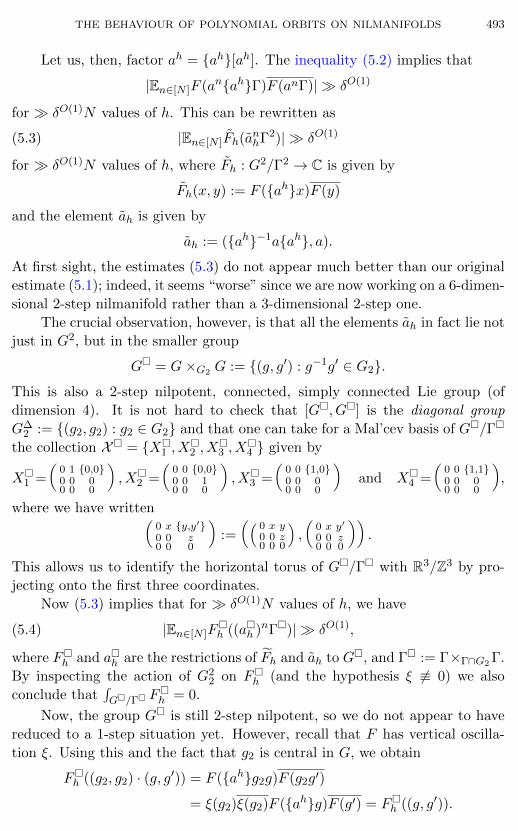
THE BEHAVIOUR OF POLYNOMIAL ORBITS ON NILMANIFOLDS 493
Let us, then, factor ah = ah[ah]. The inequality (5.2) implies that
|En∈[N ]F (anahΓ)F (anΓ)| δO(1)
for δO(1)N values of h. This can be rewritten as
(5.3) |En∈[N ]Fh(anhΓ2)| δO(1)
for δO(1)N values of h, where Fh : G2/Γ2 → C is given by
Fh(x, y) := F (ahx)F (y)
and the element ah is given by
ah := (ah−1aah, a).
At first sight, the estimates (5.3) do not appear much better than our original
estimate (5.1); indeed, it seems “worse” since we are now working on a 6-dimen-
sional 2-step nilmanifold rather than a 3-dimensional 2-step one.
The crucial observation, however, is that all the elements ah in fact lie not
just in G2, but in the smaller group
G = G×G2 G := (g, g′) : g−1g′ ∈ G2.
This is also a 2-step nilpotent, connected, simply connected Lie group (of
dimension 4). It is not hard to check that [G, G] is the diagonal group
G∆2 := (g2, g2) : g2 ∈ G2 and that one can take for a Mal’cev basis of G/Γ
the collection X = X1 , X2 , X3 , X4 given by
X1 =
Å0 1 0,00 0 00 0 0
ã, X2 =
Å0 0 0,00 0 10 0 0
ã, X3 =
Å0 0 1,00 0 00 0 0
ãand X4 =
Å0 0 1,10 0 00 0 0
ã,
where we have writtenÅ0 x y,y′0 0 z0 0 0
ã:=
Å( 0 x y0 0 z0 0 0
),
Å0 x y′
0 0 z0 0 0
ãã.
This allows us to identify the horizontal torus of G/Γ with R3/Z3 by pro-
jecting onto the first three coordinates.
Now (5.3) implies that for δO(1)N values of h, we have
(5.4) |En∈[N ]Fh ((ah )nΓ)| δO(1),
where Fh and ah are the restrictions of ‹Fh and ah to G, and Γ := Γ×Γ∩G2 Γ.
By inspecting the action of G22 on Fh (and the hypothesis ξ 6≡ 0) we also
conclude that∫G/Γ Fh = 0.
Now, the group G is still 2-step nilpotent, so we do not appear to have
reduced to a 1-step situation yet. However, recall that F has vertical oscilla-
tion ξ. Using this and the fact that g2 is central in G, we obtain
Fh ((g2, g2) · (g, g′)) = F (ahg2g)F (g2g′)
= ξ(g2)ξ(g2)F (ahg)F (g′) = Fh ((g, g′)).

494 BEN GREEN and TERENCE TAO
Thus Fh is [G, G]-invariant. In (5.4) we may therefore factor through the
projection π to obtain
|En∈[N ]Fh(nπ(ah))| δO(1)
for δO(1)N values of h, where the function Fh : R3/Z3 → C is defined by
Fh(π(x)) = Fh (xΓ).
We leave it to the reader to check that ‖Fh‖Lip = O(1) (in the general case to
follow this computation is given in more detail). Since Fh has mean zero, we
see that Fh has mean zero also.
We are now finally in a situation in which we may apply “1-step” tools.
Indeed, from Proposition 3.1 we see that for each h, there is some kh ∈ Z3,
|kh | δ−O(1), such that
‖kh · π(ah)‖R/Z δ−O(1)/N.
Pigeonholing in h, we may assume that kh = k is independent of h. Define
η : G → R/Z by
η(x) := k · π(x).
Then η is an additive homomorphism which annihilates [G, G] and Γ, and
we have
(5.5) ‖η(ah)‖R/Z δ−O(1)/N
for δO(1)N values of h ∈ [N ].
Our task now is to “piece together” these pieces of information for many
different h to deduce Proposition 5.1. We begin by factoring the character η
on G into two simpler components, which originate from G (or G2) rather
than G.
Lemma 5.2 (Decomposition of η). There exist horizontal characters η1 :
G→ R/Z and η2 : G2 → R/Z on on G and G2 respectively (thus η1 annihilates
Γ and η2 annihilates Γ ∩G2) such that
(5.6) η(g′, g) = η1(g) + η2(g′g−1)
for all (g, g′) ∈ G. Furthermore, we have |η1|, |η2| δ−O(1).
Proof. Since η is an additive homomorphism we have η(g′, g)=η((g′g−1, 1)·(g, g)) = η(g, g) + η(g′g−1, 1). Thus if we define η1(g) := η(g, g) and η2(g2) :=
η(g2, idG), then (5.6) is immediately seen to hold. Now η1 is a horizontal
character because η annihilates Γ, which contains Γ∆. Furthermore Γ also
contains (Γ∩G2)×idG, and hence η2 annihilates Γ∩G2 as claimed. The bounds
on |η1| and |η2| are left as an exercise to the reader; one may compute explicitly
with the Mal’cev bases X and X on G/Γ and G/Γ respectively.

THE BEHAVIOUR OF POLYNOMIAL ORBITS ON NILMANIFOLDS 495
Using this decomposition and the fact that, in the Heisenberg group, we
have the identity x−1yxy−1 = [x, y] since [x, y] is central, we see that
η(ah) = η1(a) + η2([a, ah]).
Now a straightforward computation with matrices confirms that if ψ(x) =
(t1, t2, t3) and ψ(y) = (u1, u2, u3), then ψ([x, y]) = (0, 0, t1u2 − t2u1), and also
that if ψ(a) = (γ1, γ2, ∗), then ψ(ah) = (γ1h, γ2h, ∗), where we do not
care about the values of the coordinates marked with an asterisk ∗. Thus if
we write γ := (γ1, γ2) = π(a) and ζ := (−γ2, γ1), then
η(ah) = k1 · γ + k2ζ · γh,
where k1, k2 = O(δ−O(1)) are the frequencies of η1, η2 respectively. Thus if
(5.5) holds, then
(5.7) ‖k1 · γ + k2ζ · γh‖R/Z δ−O(1)/N
for δO(1)N values of h.
The next proposition derives diophantine information concerning γ and
ζ from a hypothesis such as this. In fact we handle a slightly more general
situation, since this will be useful when we come to handle the general case of
Theorem 2.9. In the following proposition we shall take α = 0 and m = 2; the
proof when α = 0 is actually considerably shorter and the reader may care to
work through that case to better understand the argument.
Proposition 5.3 (Bracket polynomial lemma). Let δ ∈ (0, 1) and let
N > 1 be an integer. Suppose that α, β ∈ R and that |α| 6 1/δN . Suppose
that γ ∈ Rm/Zm and that ζ ∈ Rm satisfies |ζ| 6 1/δ. Suppose that for at least
δN values of h ∈ [N ], we have
(5.8) ‖β + αh+ ζ · γh‖R/Z 6 1/δN.
Then either |ζi| m δ−Om(1)/N for all 1 6 i 6 m, or else there is some
k ∈ Zm, |k| m δ−Om(1), such that ‖k · γ‖R/Z m δ−Om(1)/N .
Proof. If supi |ζi| 6 1/δN , then we are done, so assume this is not the
case. Then the assumption implies that ‖β + αh‖R/Z 6 (1 + m) supi |ζi| for
> δN values of h ∈ [N ]. Then Lemma 3.2 implies that there is q δ−C
such that ‖qα‖R/Z m supi |ζi|δ−C/N for some absolute constant C > 0.
Since we are assuming that |α| 6 1/δN this forces us to conclude that in fact
|α| m supi |ζi|δ−C/N unless N m δ−O(1), in which case the result is trivial
in any case.
Split [N ] into intervals of length between N ′ and 2N ′, where N ′ :=
cmδC+1N and cm > 0 is a small number to be chosen later. By the pigeonhole
principle, we can find one of these intervals I in which there are > δ|I| values
of h such that (5.8) holds. If cm is chosen sufficiently small, then αh does not
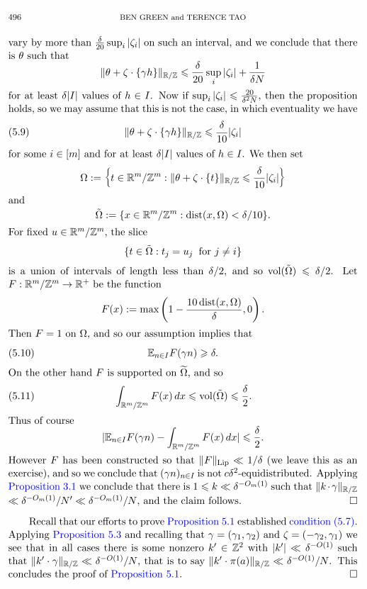
496 BEN GREEN and TERENCE TAO
vary by more than δ20 supi |ζi| on such an interval, and we conclude that there
is θ such that
‖θ + ζ · γh‖R/Z 6δ
20supi|ζi|+
1
δN
for at least δ|I| values of h ∈ I. Now if supi |ζi| 6 20δ2N
, then the proposition
holds, so we may assume that this is not the case, in which eventuality we have
(5.9) ‖θ + ζ · γh‖R/Z 6δ
10|ζi|
for some i ∈ [m] and for at least δ|I| values of h ∈ I. We then set
Ω :=
ßt ∈ Rm/Zm : ‖θ + ζ · t‖R/Z 6
δ
10|ζi|™
and
Ω := x ∈ Rm/Zm : dist(x,Ω) < δ/10.For fixed u ∈ Rm/Zm, the slice
t ∈ Ω : tj = uj for j 6= i
is a union of intervals of length less than δ/2, and so vol(Ω) 6 δ/2. Let
F : Rm/Zm → R+ be the function
F (x) := max
Ç1− 10 dist(x,Ω)
δ, 0
å.
Then F = 1 on Ω, and so our assumption implies that
(5.10) En∈IF (γn) > δ.
On the other hand F is supported on ‹Ω, and so
(5.11)
∫Rm/Zm
F (x) dx 6 vol(Ω) 6δ
2.
Thus of course
|En∈IF (γn)−∫Rm/Zm
F (x) dx| 6 δ
2.
However F has been constructed so that ‖F‖Lip 1/δ (we leave this as an
exercise), and so we conclude that (γn)n∈I is not cδ2-equidistributed. Applying
Proposition 3.1 we conclude that there is 1 6 k δ−Om(1) such that ‖k ·γ‖R/Z δ−Om(1)/N ′ δ−Om(1)/N , and the claim follows.
Recall that our efforts to prove Proposition 5.1 established condition (5.7).
Applying Proposition 5.3 and recalling that γ = (γ1, γ2) and ζ = (−γ2, γ1) we
see that in all cases there is some nonzero k′ ∈ Z2 with |k′| δ−O(1) such
that ‖k′ · γ‖R/Z δ−O(1)/N , that is to say ‖k′ · π(a)‖R/Z δ−O(1)/N . This
concludes the proof of Proposition 5.1.
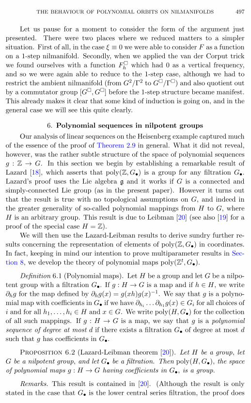
THE BEHAVIOUR OF POLYNOMIAL ORBITS ON NILMANIFOLDS 497
Let us pause for a moment to consider the form of the argument just
presented. There were two places where we reduced matters to a simpler
situation. First of all, in the case ξ ≡ 0 we were able to consider F as a function
on a 1-step nilmanifold. Secondly, when we applied the van der Corput trick
we found ourselves with a function Fh which had 0 as a vertical frequency,
and so we were again able to reduce to the 1-step case, although we had to
restrict the ambient nilmanifold (from G2/Γ2 to G/Γ) and also quotient out
by a commutator group [G, G] before the 1-step structure became manifest.
This already makes it clear that some kind of induction is going on, and in the
general case we will see this quite clearly.
6. Polynomial sequences in nilpotent groups
Our analysis of linear sequences on the Heisenberg example captured much
of the essence of the proof of Theorem 2.9 in general. What it did not reveal,
however, was the rather subtle structure of the space of polynomial sequences
g : Z → G. In this section we begin by establishing a remarkable result of
Lazard [18], which asserts that poly(Z, G•) is a group for any filtration G•.
Lazard’s proof uses the Lie algebra g and it works if G is a connected and
simply-connected Lie group (as in the present paper). However it turns out
that the result is true with no topological assumptions on G, and indeed in
the greater generality of so-called polynomial mappings from H to G, where
H is an arbitrary group. This result is due to Leibman [20] (see also [19] for a
proof of the special case H = Z).
We will then use the Lazard-Leibman results to derive sundry further re-
sults concerning the representation of elements of poly(Z, G•) in coordinates.
In fact, keeping in mind our intention to prove multiparameter results in Sec-
tion 8, we develop the theory of polynomial maps poly(Zt, G•).
Definition 6.1 (Polynomial maps). Let H be a group and let G be a nilpo-
tent group with a filtration G•. If g : H → G is a map and if h ∈ H, we write
∂hg for the map defined by ∂hg(x) = g(xh)g(x)−1. We say that g is a polyno-
mial map with coefficients in G• if we have ∂hi . . . ∂h1g(x) ∈ Gi for all choices of
i and for all h1, . . . , hi ∈ H and x ∈ G. We write poly(H,G•) for the collection
of all such mappings. If g : H → G is a map, we say that g is a polynomial
sequence of degree at most d if there exists a filtration G• of degree at most d
such that g has coefficients in G•.
Proposition 6.2 (Lazard-Leibman theorem [20]). Let H be a group, let
G be a nilpotent group, and let G• be a filtration. Then poly(H,G•), the space
of polynomial maps g : H → G having coefficients in G•, is a group.
Remarks. This result is contained in [20]. (Although the result is only
stated in the case that G• is the lower central series filtration, the proof does

498 BEN GREEN and TERENCE TAO
not use this fact.) Our proof is a little different, relying on the machinery of
Host-Kra cube groups. These were featured for the first time in [15, §§5, 11] and
were discussed subsequently in [11, App. E]. See also the recent preprint [16].
We thank Sasha Leibman for helpful conversations concerning these methods.
One should mention at this point the Hall-Petresco theorem [14], [27],
which established a special case of the Lazard-Leibman theorem. This theorem
states that if G• is the lower central series filtration, then the sequence n 7→anbn lies in poly(Z, G•) for any a, b ∈ G.
In this section it is convenient to generalise the notion of a filtration some-
what. By a prefiltration G• on a nilpotent group G we mean a sequence
G ⊇ G0 ⊇ G1 ⊇ · · · ⊇ Gd ⊇ idG
of subgroups with the property that [Gi, Gj ] ⊆ Gi+j for all i, j > 0. The only
difference between a prefiltration and a filtration (cf. Definition 1.1) is that we
no longer require that G = G0 = G1. The definition of poly(H,G•) extends in
a completely obvious way to prefiltrations.
For each integer k > 0, we are going to define the Host-Kra cube group
HKk(G•) associated to the prefiltration G•. This will be a subgroup of G0,1k,
the product of 2k copies of G indexed by the cube 0, 1k. Before giving the
definition, we need to set up some nomenclature concerning these cubes.
Each element ω ∈ 0, 1k corresponds in an obvious way to a subset of [k],
and we write ω ⊆ ω′ when the corresponding sets are nested. An upper face F
is a subset of 0, 1k of the form F (ω0) := ω ∈ 0, 1k : ω ⊇ ω0. There are, of
course, 2k upper faces, one for each ω0 ∈ 0, 1k. The codimension codim(F )
of F is simply the number of ones in ω0. Note that if F, F ′ are two upper faces,
then F ∩F ′ is also an upper face, and codim(F ∩F ′) 6 codim(F )+codim(F ′).
Given an upper face F and an element x ∈ G, we write xF for the element
of G0,1k
defined by
(xF )ω =
x if ω ∈ F ,
idG otherwise.
Write ΓF for the subgroup of G0,1k
consisting of all elements xF with x ∈Gcodim(F ), where Gi is the ith group in the prefiltration G•; we call such a
group an upper face group.
Definition 6.3 (Host-Kra cube group). Let G• be a prefiltration on a nilpo-
tent group G, and let k > 0 be an integer. Then the Host-Kra cube group
HKk(G•) is the subgroup of G0,1k
generated by the upper face groups ΓF .
The Host-Kra cube group can, it turns out, be described in a rather ex-
plicit way. Write ≺ for the reverse lexicographic ordering on 0, 1k; thus
ω ≺ ω′ if an only if there is some j such that ωj < ω′j and ωi = ω′i for

THE BEHAVIOUR OF POLYNOMIAL ORBITS ON NILMANIFOLDS 499
i = j + 1, . . . , k. This induces an ordering on the upper faces F . We write
F (ω) F (ω′) if and only if ω ≺ ω′. Let F0 ≺ F1 ≺ · · · ≺ F2k−1 be the
complete list of upper faces in this order; thus F0 = 1k and F2k−1 = 0, 1k.
Lemma 6.4 (Description of Host-Kra cube group). We have
HKk(G•) = ΓF0 · ΓF1 · . . .ΓF2k−1.
That is, every element of HKk(G) may be written as γF00 . . . γF
2k−1
2k−1, where
γi ∈ Gcodim(Fi). The representation is in fact unique.
Proof. The key point here is the inclusion
(6.1) [ΓF ,ΓF ′ ] ⊆ ΓF∩F ′ .
This follows immediately from the fact that
[Gcodim(F ), Gcodim(F ′)] ⊆ Gcodim(F )+codim(F ′) ⊆ Gcodim(F∩F ′).
Using this fact repeatedly, we shift all elements coming from ΓF0 to the left.
We then shift all elements coming from ΓF1 to the left, and so on. We leave
the routine details and the proof that the representation is unique (which we
do not actually need) to the reader.
Host-Kra cube groups and polynomial maps. It is now time to develop
the link between Host-Kra cube groups HKk(G•) and polynomial maps g ∈poly(H,G•). To do this we introduce a the notion of a parallelepiped on H.
This is an element in H0,1k
of the form (xhω)ω∈0,1k , where x ∈ H, h =
(h1, . . . , hk) is a k-tuple of elements of H, and hω := hω11 . . . hωk
k . For example
the tuple (x, xh1, xh2, xh1h2) is a parallelepiped in H0,12, and (x, xh1, xh2,
xh1h2, xh3, xh1h2, xh2h3, xh1h2h3) is a parallelepiped in H0,13. Write H [k]
for the set of parallelepipeds in H0,1k. (If H is abelian, H [k] is actually a
group, but this need not be the case in general and in any case is not important
here.)
Suppose that g : H → G is a map. Then for any k > 0, there is an obvious
induced map g0,1k
: H0,1k → G0,1
k.
Proposition 6.5 (Characterisation of polynomial maps). Suppose that
H is a group, that G is a nilpotent group together with a prefiltration G•, and
that g : H → G. Then g lies in poly(H,G•) if and only if g0,1k
maps H [k] to
HKk(G•) for all k > 0.
Remark. The reader might find it useful, as an exercise to get to grips
with the notation, to verify this in the case H = G and g being the identity
mapping.
We note that Proposition 6.2 is an immediate consequence of Proposi-
tion 6.5. Indeed if g0,1k
and g0,1k
both map H [k] to HKk(G•), then so does
(gg)0,1k, since HKk(G•) is a group.
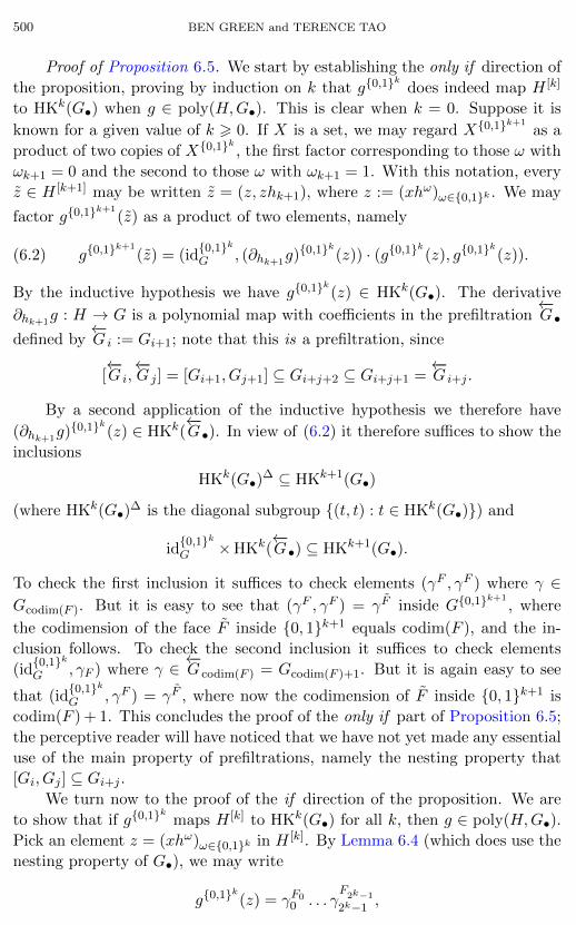
500 BEN GREEN and TERENCE TAO
Proof of Proposition 6.5. We start by establishing the only if direction of
the proposition, proving by induction on k that g0,1k
does indeed map H [k]
to HKk(G•) when g ∈ poly(H,G•). This is clear when k = 0. Suppose it is
known for a given value of k > 0. If X is a set, we may regard X0,1k+1
as a
product of two copies of X0,1k, the first factor corresponding to those ω with
ωk+1 = 0 and the second to those ω with ωk+1 = 1. With this notation, every
z ∈ H [k+1] may be written z = (z, zhk+1), where z := (xhω)ω∈0,1k . We may
factor g0,1k+1
(z) as a product of two elements, namely
(6.2) g0,1k+1
(z) = (id0,1kG , (∂hk+1
g)0,1k(z)) · (g0,1k(z), g0,1
k(z)).
By the inductive hypothesis we have g0,1k(z) ∈ HKk(G•). The derivative
∂hk+1g : H → G is a polynomial map with coefficients in the prefiltration
←−G•
defined by←−G i := Gi+1; note that this is a prefiltration, since
[←−G i,←−G j ] = [Gi+1, Gj+1] ⊆ Gi+j+2 ⊆ Gi+j+1 =
←−G i+j .
By a second application of the inductive hypothesis we therefore have
(∂hk+1g)0,1
k(z) ∈ HKk(
←−G•). In view of (6.2) it therefore suffices to show the
inclusions
HKk(G•)∆ ⊆ HKk+1(G•)
(where HKk(G•)∆ is the diagonal subgroup (t, t) : t ∈ HKk(G•)) and
id0,1kG ×HKk(
←−G•) ⊆ HKk+1(G•).
To check the first inclusion it suffices to check elements (γF , γF ) where γ ∈Gcodim(F ). But it is easy to see that (γF , γF ) = γF inside G0,1
k+1, where
the codimension of the face F inside 0, 1k+1 equals codim(F ), and the in-
clusion follows. To check the second inclusion it suffices to check elements
(id0,1kG , γF ) where γ ∈
←−G codim(F ) = Gcodim(F )+1. But it is again easy to see
that (id0,1kG , γF ) = γF , where now the codimension of F inside 0, 1k+1 is
codim(F ) + 1. This concludes the proof of the only if part of Proposition 6.5;
the perceptive reader will have noticed that we have not yet made any essential
use of the main property of prefiltrations, namely the nesting property that
[Gi, Gj ] ⊆ Gi+j .We turn now to the proof of the if direction of the proposition. We are
to show that if g0,1k
maps H [k] to HKk(G•) for all k, then g ∈ poly(H,G•).
Pick an element z = (xhω)ω∈0,1k in H [k]. By Lemma 6.4 (which does use the
nesting property of G•), we may write
g0,1k(z) = γF0
0 . . . γF2k−1
2k−1,

THE BEHAVIOUR OF POLYNOMIAL ORBITS ON NILMANIFOLDS 501
where γi ∈ Gcodim(Fi). Write ηj := γF2j−1
2j−1 . . . γF2j−1
2j−1 , j = 1, . . . , k, so that
(6.3) g0,1k(z) = γ1k
0 η1 . . . ηk.
One may check that the ηi enjoy the following support properties: (ηi)ω = idGunless ωi+1, . . . , ωk are all nonzero, and (ηi)ω = (ηi)ω′ if ω, ω′ differ only in
the ωi coordinate. One may now examine (6.3) coordinatewise, peeling off
ηk, ηk−1, . . . in turn, eventually to conclude that
γ0 = ∂h1 . . . ∂hkg(x).
Now we know that γ0 ∈ Gcodim(F0) = Gk, and thus we have proved that
∂h1 . . . ∂hkg takes values in Gk, as required.
Polynomial maps in coordinates. From now on we specialise to the case
of polynomial maps from Zt to G and revert to dealing with filtrations as
opposed to prefiltrations. Our aim in this section is to describe the elements of
poly(Zt, G•) using the Mal’cev coordinate map ψ : G → Rm relative to some
Mal’cev basis X for G/Γ adapted to the filtration G•.
Definition 6.6 (Multi-binomial coefficients). Let t > 1 be an integer. Sup-
pose that ~n = (n1, . . . , nt) and that ~j = (j1, . . . , jt) ∈ Zt>0 is a set of indices.
Then we write Ç~n~j
å:=
t∏i=1
Çniji
å.
A version of the following lemma may be found in [23, §4].
Lemma 6.7 (Description of poly(Zt, G•) in bases). Suppose that G/Γ is
a nilmanifold of dimension m and that X is a Mal’cev basis for G/Γ adapted
to some filtration G•. Then g ∈ poly(Zt, G•) if and only if the coordinates
ψ(g(n)) have the form
ψ(g(n)) =∑~j
t~j
Ç~n~j
å,
where each t~j lies in Rm and is such that (t~j)i = 0 if i 6 m − m|~j|, where
|~j| := j1 + · · ·+ jt.
Remark. The presence of the discrete subgroup Γ is not at all relevant to
this lemma; however we have only defined Mal’cev bases in this context.
Proof. We start with the if direction. If g(n) has the form stated, then it
is a product of sequences of the form ~n 7→ a(~n~j), where a ∈ G|~j|. By the group
property of poly(Zt, G•) it therefore suffices to establish the result in the case
that g(~n) is actually equal to such a sequence. By induction one sees that
the derivative ∂h1 . . . ∂hkg(~n) equals ap(h1,...,hk;~n), where the maximal degree

502 BEN GREEN and TERENCE TAO
α1 + · · ·+αt of a monomial nα11 . . . nαt
t appearing in p is at most max(|~j|−k, 0).
Thus we see that this derivative lies in G|~j| if k 6 |~j| and is zero otherwise. It
follows that g ∈ poly(Zt, G•).To prove the only if direction, let hj ⊂ g be the subspace
hj := Span(Xj+1, . . . , Xm)
and set Hj := exp(hj). By the nesting property of the Mal’cev basis X (see
(A.1)), we see that Hj CG.
Suppose as a hypothesis for downward induction on k that the statement
has been proved for all g ∈ poly(Zt, G•) with g(~n) ∈ Hk for all ~n, for a certain
value of k. This is trivial for k = m, in which case g(~n) = idG. Suppose
that g(~n) ∈ Hk−1 for all ~n. Let π : Hk−1 → Hk−1/Hk∼= R be the natural
projection. Then pk−1(~n) := π(g(~n)Γ) is a polynomial map from Rt to R.
Suppose that k − 1 < m −mi and that i is minimal subject to this property.
Then for any h1, . . . , hi ∈ Zt, we have ∂h1 . . . ∂hig ∈ Gi = Hm−mi , and therefore
∂h1 . . . ∂hipk−1(~n) = 0. Thus the total degree of any monomial in pk−1 is at
most i− 1. Therefore we may write the sequence h(~n) defined by
h(~n) := exp(Xk−1)pk−1(~n)
as a product of sequences exp(Xk−1)t~j(
~n~j) with |~j| 6 i− 1. By the minimality
of i we have Xk−1 ∈ gi−1, and so each of these sequences lies in poly(Zt, G•),and hence so does h. It follows that the sequence g(n) := g(n)h(n)−1 lies
in poly(Zt, G•). But this new sequence g has g(n) ∈ Hk, and hence we may
proceed by induction.
A useful and easily-derived corollary of Lemma 6.7 is that poly(Zt, G•) is
closed under dilations.
Corollary 6.8 (Dilation of polynomial sequences). Suppose that g ∈poly(Zt, G•) and that a1, . . . , at, b1, . . . , bt ∈ Z. Then the sequence ~n 7→ g(a1 +
b1n1, . . . , at + btnt) also lies in G•.
We remarked in the introduction that a sequence g : Z→ G is polynomial
with coefficients in some filtration G• if and only if g has the form
(6.4) g(n) = ap1(n)1 . . . a
pk(n)k
for polynomials p1, . . . , pk with integer coefficients. Although this result is not
required in the paper, it is certainly conceivable that one might wish to apply
the main theorems of the paper to a sequence that is presented in an explicit
form such as (6.4) and does not obviously satisfy the more abstract condition
of Definition 1.8.
The fact that every polynomial sequence has the form (6.4) is an easy
consequence of Lemma 6.7. To establish the converse, consider first the lower
THE BEHAVIOUR OF POLYNOMIAL ORBITS ON NILMANIFOLDS 503
central series filtration G• which has degree s, the step of the nilpotent Lie
group G. Let d be the maximum degree occurring amongst the polynomials piand define a finer filtration G′• of degree sd by setting G′i := Gdi/de. This is a
filtration since
[G′i, G′j ] = [Gdi/de, Gdj/de] ⊆ Gdi/de+dj/de ⊆ Gd(i+j)/de = G′i+j .
Any sequence of the form n 7→ a(nj), j 6 d has coefficients in G′• since G′i = G
for i = 0, 1, . . . , d and the (d + 1)st derivative of such a sequence is trivial.
Since g is a product of such sequences and poly(Z, G′•) is a group we see that
g ∈ poly(Z, G′•).We note that if G/Γ has a Q-rational Mal’cev basis adapted to the lower
central series then, by the results of the appendix, there is a QOd,s(1)-rational
Mal’cev basis for G/Γ adapted to G′•.
We leave it to the reader to formulate and prove an analogous result for
polynomial mappings from Zt to G.
7. The general case of the main theorem
We are now in a position to attack the general case of Theorem 2.9. Our
analysis of the Heisenberg example in Section 5 suggested that the argument
will involve an induction on the degree d of G•. In that case there were two
different scenarios in which we reduced from the case d = 2 to the case d = 1.
Whilst the same is true in general, the introduction of genuinely polynomial
sequences (rather than just linear ones) necessitates a further inductive loop
on the quantity m∗ := mab −mlin, which we call the nonlinearity degree. To
see why, consider the following slightly informal example.
Example. Let G/Γ be the Heisenberg example, and let g(n) =
Å1 α1 α30 1 α20 0 1
ãn,
where α1, α2, and α3 are highly independent over Q. Then there is no hori-
zontal character η of low frequency such that ‖η g‖C∞[N ] is small.
Now we have ∂g = g and ∂ig = idG for i > 2, and so g has coefficients
in the subgroup sequence G• defined by G(0) := G(1) := G(2) := G, G(3) :=
G(4) := G2, and G(i) := idG for i > 5. With this choice we have G = G×G.
However gh takes values in G×G2 G, and hence η gh = 0 for any horizontal
character η with frequency of the form (a, b,−a,−b) ∈ Z4. Thus, a lack of
uniform distribution for gh does not imply lack of uniform distribution for g.
The problem in the above example is that the filtration G• was far too
“coarse” to accurately capture the differential structure of the sequence g.
Indeed g also takes values in the minimal (lower central series) filtration, as
we saw in Section 5.
In the light of the above example, we can expect that it will sometimes
be necessary to pass to a “finer” filtration of the same degree d in order to

504 BEN GREEN and TERENCE TAO
properly capture the differential structure of g. This finer filtration will have
a smaller value of the nonlinearity degree m∗, and thus we introduce an extra
inductive loop to incorporate this parameter. To be precise we shall prove, by
induction on d and m∗, the following slight variant of Theorem 2.9.
Theorem 7.1 (Variant of Main Theorem). Let m, d > 0 be integers with
m∗ 6 m. Let 0 < δ < 1/2, and suppose that N > 1. Suppose that G/Γ is a
nilmanifold and that G• is a filtration of degree d and with nonlinearity degree
m∗. Suppose that X is a 1/δ-rational Mal’cev basis adapted to G•, and suppose
that g ∈ poly(Z, G•). If (g(n)Γ)n∈[N ] is not δ-equidistributed, then there is a
horizontal character η with 0 < |η| δ−Om,m∗,d(1) such that
‖η g‖C∞[N ] δ−Om,m∗,d(1).
It is clear that this does imply Theorem 2.9, since the dependence of the
O(1) exponents on m∗ may be suppressed once Theorem 7.1 has been proven
by induction. In our proof there will be an outer inductive loop over d and an
inner one over m∗. In other words we shall assume that Theorem 7.1 holds for
all pairs (d′,m′∗) in which either d′ < d or for which d′ = d and m′∗ < m∗, and
deduce the case (d,m∗).
Henceforth we allow all constants implicit in the or O-notation to de-
pend on d,m and m∗.
We begin with some simple reductions. By Lemma 3.7 we may assume
that the orbit (g(n)Γ)n∈[N ] is not δO(1)-equidistributed along some vertical
frequency ξ ∈Zmd with |ξ| δ−O(1). Thus there is some function F :G/Γ→Cwith ‖F‖Lip 6 1 and vertical frequency ξ such that
(7.1) |En∈[N ]F (g(n)Γ)−∫G/Γ
F | δO(1).
If ξ = 0 then F is Gd-invariant and we may descend to G/Gd, together with the
filtration G•/Gd which has length d− 1, and invoke our inductive hypothesis.
We pause to give the rather straightforward details.
Write G := G/Gd and Γ := Γ/(Γ ∩ Gd). Then G/Γ is a nilmanifold
togther with a filtration G• of length d− 1, where Gi := Gi/Gd. The Mal’cev
basis X = X1, . . . , Xm may be reduced to give a 1δ -rational Mal’cev basis
X = X1, . . . , Xm for G/Γ adapted to G•, where m := m−md.
Write g : Z → G for the reduction of g(mod Gd). By the Gd-invariance
the function F descends to a Lipschitz function F : G/Γ → C with ‖F‖Lip 6‖F‖Lip, and so (7.1) implies that∣∣∣∣∣En∈[N ]F (g(n)Γ)−
∫G/Γ
F
∣∣∣∣∣ > δ‖F‖Lip.

THE BEHAVIOUR OF POLYNOMIAL ORBITS ON NILMANIFOLDS 505
(Here we have used the fact that normalised Haar measure on G/Γ is be ob-
tained by quotienting that on G/Γ by Gd.)
We may now apply the inductive hypothesis to obtain a horizontal char-
acter η : G→ C on G of frequency magnitude 0 < |η| δ−O(1) such that
‖η g‖C∞[N ] δ−O(1).
If we let η : G → C be the horizontal character on G defined by η(x) = η(x),
then we have η g = η g and |η| = |η|. This concludes the proof in the case
ξ = 0.
Suppose henceforth that ξ 6= 0. Since F has ξ as a vertical frequency,
(7.1) becomes
(7.2) |En∈[N ]F (g(n)Γ)| δO(1).
We proceed initially with two additional reductions. The first is to the case
g(0) = idG. Factorise g(0) = g(0)[g(0)] as in Lemma A.14. Set g(n) :=
g(0)−1g(n)g(0)−1g(0). Then we have |En∈[N ]F (g(n)Γ)| > δ, where F (x) :=
F (g(0)x). But F still has vertical oscillation ξ and, by Lemma A.5, it has
Lipschitz constant O(1). Noting that ‖η g‖C∞[N ] = ‖η g‖C∞[N ] we see that
if we have Theorem 7.1 for g then we also have it for g.
The second reduction is to the case when |ψ(g(1))| 6 1. (This is needed
in the lead up to (7.16).) To do this, factorise g(1) = g(1)[g(1)] as in
Lemma A.14. Set g(n) := g(n)[g(1)]−n. Then g(n)Γ = g(n)Γ, g(0) = idG,
g ∈ poly(Z, G•), and π(g(n)Γ) = π(g(n)Γ), so proving Theorem 7.1 for g is
equivalent to proving it for g.
Henceforth we assume g(0) = idG and |ψ(g(1))| 6 1.
As in Section 5 we apply Van der Corput’s Lemma (Corollary 4.2) to (7.2)
to deduce that for δO(1)N values of h, we have
(7.3) |En∈[N ]F (g(n+ h)Γ)F (g(n)Γ)| δO(1).
For each fixed h, this may be interpreted as a statement about the polynomial
sequence (g(n + h), g(n)) on the product group G2. However, guided by our
experience with the Heisenberg group, it is natural to try and interpret it as a
sequence on a somewhat smaller group. To this end, we define the nonlinear
part g2 of g by
(7.4) g2(n) := g(n)g(1)−n.
Motivated by what we did in Section 5, we may then rewrite (7.3) in the form
(7.5) |En∈[N ]Fh(gh(n)Γ2)| δO(1),
where
Fh(x, y) := F (g(1)hx)F (y)
506 BEN GREEN and TERENCE TAO
and
(7.6) gh(n) := (g(1)h−1g2(n+ h)g(1)ng(1)h, g2(n)g(1)n).
It turns out that gh takes values in G := G ×G2 G, just as we found in our
analysis of the Heisenberg case. To prove this, note that G2 ⊇ [G,G] and so
G becomes abelian after quotienting out by the normal subgroup G2. Thus we
need only prove that g2(n) ∈ G2 for all n. We have ∂2g(n) = idG modulo G2.
Since g(0) = idG, this implies by an easy induction that g(n) = g(1)n modulo
G2, and so g2 does indeed take values in G2.
We may therefore replace (7.5) by
(7.7) |En∈[N ]Fh (gh (n)Γ)| δO(1)
by restricting everything in that equation to an object on G.
Note that, exactly as in the Heisenberg case, Fh is invariant under G∆d =
(gd, gd) : gd ∈ Gd. Indeed, since Gd is central in G, we have
Fh ((gd, gd) · x) = F (g(1)hgdx)F (gdx′)
= e(ξ(gd))e(−ξ(g′d))F (g(1)hx)F (x′)
= Fh (x).
Thus Fh descends to a function Fh on G := G/G∆d and we may write (7.7)
as
(7.8) |En∈[N ]Fh (gh (n)Γ)| δO(1),
where Γ := Γ/(Γ ∩G∆d ).
The next proposition is central to our whole argument in that it clarifies
the sense in which G is “less complex” than G.
Proposition 7.2 (Reduction in degree). Define (G)i := Gi×Gi+1Gi for
i = 1, . . . , d. Then (G)• is a filtration on G of degree d. Since (G)d = G∆d ,
it descends under quotienting by G∆d to a filtration (G)• of degree d−1 on G.
Each polynomial sequence gh lies in poly(Z, (G)•), and hence each reduced
polynomial sequence gh lies in poly(Z, (G)•).
Proof. We start with a lemma.
Lemma 7.3. Suppose that H1, H2 and K1,K2 are normal subgroups of a
group G, that H1, H2 generate a group H , and that K1,K2 generate a group
K . Then [H,K] is generated by the groups [Hi,Kj ], 1 6 i, j 6 2.
Proof. The groups [Hi,Kj ] are all normal, and thus the group they gen-
erate is also normal. If we quotient by that group, then H1, H2 commute with
K1,K2, and thus H commutes with K. The claim follows.
THE BEHAVIOUR OF POLYNOMIAL ORBITS ON NILMANIFOLDS 507
Now observe that (G)i is generated by G2i+1 and G4i . In view of the
lemma, it therefore suffices to establish that all four of the quantities
[G4i , G4j ], [G4i , G
2j+1], [G2
i+1, G4j ], [G2
i+1, G2j+1]
lie in Gi+j . Using the fact that G• is a filtration, the first quantity is manifestly
contained in G4i+j and the last three lie in G2i+j+1. It follows immediately that
(G)• is indeed a filtration.
Next we show that gh ∈ poly(Z, (G)•). Here we make serious use of the
fact that poly(Z, G•) is a group for the first time. Recall that
(7.9) gh (n) :=Äg(1)h−1g2(n+ h)g(1)ng(1)h, g2(n)g(1)n
ä.
Now poly(Z, (G)•) is a group, and it is also closed under conjugation by
elements of G2. Since (g(1)n, g(1)n) is obviously in poly(Z, (G)•), it suffices
to check that (g2(n+ h), g2(n)) ∈ poly(Z, (G)•). Of course, g2 ∈ poly(Z, G•)
and hence, by Lemma 6.7, it is a product of elements g(ni)i with gi ∈ Gi. It
therefore suffices to show that (g(n+h
i )i , g
(ni)i ) ∈ (G)•. Taking jth derivatives,
it suffices to check that g(n+hi−j )
i ≡ g( ni−j)i (mod Gj+1). For j < i, this follows
from the fact that gi ∈ Gi, whilst for j > i it is trivial.
In order to apply the inductive hypothesis, we must specify a Mal’cev basis
X for G/Γ adapted to the sequence (G)•, and it must then be checked
that Fh is Lipschitz with respect to the metric dX . These are rather tedious
matters, and we recommend that the reader take the following lemma on trust
on a first reading of the paper.
Lemma 7.4 (Rationality bounds for the relative square). There is an
O(δ−O(1))-rational Mal’cev basis X = X1 , . . . , Xm for G/Γ adapted to
the filtration (G)• with the property that ψX(x, x′) is a polynomial of degree
O(1) with rational coefficients of height δ−O(1) in the coordinates ψ(x), ψ(x′).
With respect to the metric dX , we have ‖Fh ‖Lip δ−O(1) uniformly in h.
Proof. We consider G as a subgroup of G×G. Recall (cf. Definition A.7)
the definition of a weak basis. It is clear that
X × X = (X1, 0), (0, X1), . . . , (Xm, 0), (0, Xm)
is a δ−O(1)-rational weak basis for G/Γ × G/Γ and that each of the groups
(G)i := Gi ×Gi+1 Gi is δ−O(1)-rational with respect to this basis. By Propo-
sition A.10 it follows that there is a Mal’cev basis X = X1 , . . . , Xm for
G/Γ, adapted to the filtration (G)•, with the property that each Xi is a
δ−O(1)-rational combination of the elements of X ×X . By adding the elements
(X1, 0), . . . , (Xmlin, 0) to X, we obtain a weak basis Y for G/Γ×G/Γ which
508 BEN GREEN and TERENCE TAO
enjoys the nesting property (A.1). From Lemma A.2 it follows that each coor-
dinate of ψY(x, x′) is a polynomial of degree O(1) and with coefficients δ−O(1)
in the coordinates ψX×X (x, x′). Restricting to those pairs (x, x′) which lie in
G, we obtain the stated property.
Recall that Fh (x) = F (g(1)hx)F (x′). Now by definition we have
|ψX (g(1)h)| 6 1. By Lemma A.5 (and Lemma A.14, which guarantees that
every x ∈ G/Γ has a representative with coordinates bounded by O(1)), we
see that (x, x′) 7→ F (g(1)hx)F (x′) defines a function on G×G whose Lips-
chitz constant with respect to the product metric d × d is δ−O(1). Now by
Lemma A.6 and the construction of X we therefore have ‖Fh ‖Lip δ−O(1)
where, remember, the Lipschitz constant is being computed with respect to
the metric dX .
Let us now resume the discussion starting from (7.8). We begin by repris-
ing some of the straightforward arguments at the start of the section (where
we dealt with the case ξ = 0). By reducing the first m := m −md elements
of X, we obtain an O(δ−O(1))-rational Mal’cev basis X = X1 , . . . , Xm
for G/Γ adapted to the filtration (G)•. With respect to the metric dX
we have ‖Fh ‖Lip δ−O(1).
Since (G)• has degree d−1, our inductive hypothesis is applicable and we
conclude that for δO(1) values of h ∈ [N ], there is some horizontal character
ηh : G → R/Z with 0 < |ηh| δ−Om(1) and
‖ηh gh ‖C∞[N ] δ−Om(1).
By pigeonholing in h we may assume that η = ηh is independent of h. Writing
η : G → R/Z for the horizontal character defined by η(x) = η(x), we see that
0 < |η| δ−Om(1) and that
(7.10) ‖η gh ‖C∞[N ] δ−Om(1).
The next lemma, which is almost identical to Lemma 5.2, allows us to
write η in terms of maps defined on G rather than G.
Lemma 7.5. We have a decomposition η(g′, g) = η1(g) + η2(g′g−1) for
all (g′, g) ∈ G, where η1 : G → R/Z is a horizontal character on G, and
η2 : G2 → R/Z is a horizontal character on G2 which also annihilates [G,G2].
Furthermore, we have |η1|, |η2| δ−O(1).
Proof. If we define η1(g) := η(g, g) and η2(g2) := η(g2, idG) for g ∈ G and
g2 ∈ G2, then the decomposition follows since η is an additive homomorphism.
Since η annihilates [G, G], which contains [G∆, G2× idG] = [G,G2]× idG, we
see that η2 annihilates [G,G2]; since η annihilates Γ, which contains both Γ∆
and (Γ∩G2)× idG, we see that η1 and η2 annihilate Γ and Γ∩G2 respectively.

THE BEHAVIOUR OF POLYNOMIAL ORBITS ON NILMANIFOLDS 509
It remains to check the boundedness properties. Writing
η(x, x′) = k · ψX(x, x′),
where k ∈ Zm , we have by definition that |k| δ−O(1). The integer vectors
k1 and k2 used to define |η1| and |η2| are then given by
k1 · ψ(x) = η1(x) = η(x, x) = k · ψX(x, x)
and
k2 · ψ(x) = η2(x) = η(x, idG) = k · ψX(x, idG).
The fact that |k1|, |k2| δ−O(1) now follows immediately from the fact, es-
tablished in Lemma 7.4, that ψX(x, x′) is a polynomial of degree O(1) with
rational coefficients of height O(δ−O(1)) in the coordinates ψ(x), ψ(x′).
Now let us return to (7.10) and reinterpret this in terms of the decom-
position of η just given. Recalling the formula (7.9) for gh (n), we therefore
have
η(gh (n)) = η1(g(n)) + η2(g(1)h−1g2(n+ h)g(1)ng(1)hg(1)−ng2(n)−1)
which, since η2 vanishes on [G,G(2)], is equal to
η1(g(n)) + η2(g2(n+ h)g(1)h−1g(1)ng(1)hg(1)−ng2(n)−1)
= η1(g(n)) + η2(g2(n+ h))− η2(g2(n)) + η2(g(1)h−1g(1)ng(1)hg(1)−n).
One easily verifies by induction on n that y−1xnyx−n ≡ [x, y]n(mod [G, [G,G]]).
Since η2 annihilates [G,G2], which contains [G, [G,G]], we can therefore sim-
plify the above a little further to
η(gh (n)) = η1(g(n)) + η2(g2(n+ h))− η2(g2(n)) + nη2([g(1), g(1)h])(7.11)
:= P (n) +Q(n+ h)−Q(n) + σ(h)n,
where P,Q : Z→ R/Z are polynomial sequences of degree at most d.
The next lemma is specifically designed to handle the situation that has
arisen here. In this lemma it is convenient to reprise a notation from earlier
papers of ours (such as [10]): if α ∈ R/Z and Q > 1, we write ‖α‖R/Z,Q :=
inf16q6Q ‖qα‖R/Z. In a similar spirit, for any f : Z→ R/Z, define
‖f‖C∞[N ],Q := inf16q6Q
‖qf‖C∞[N ].
Lemma 7.6 (Polynomials lemma). Suppose that P,Q : Z → R/Z are
polynomial sequences of degree at most d with P (0) = 0 and Q(0) = ∂Q(0) = 0
and that σ : [N ]→ R/Z is an arbitrary map. Suppose that there are δO(1)N
values of h ∈ [N ] such that
‖P (n) +Q(n+ h)−Q(n) + σ(h)n‖C∞[N ] δ−O(1).

510 BEN GREEN and TERENCE TAO
Then ‖∂iQ‖R/Z,δ−O(1) δ−O(1)/N i for i > 3, and
‖P (1) + αh+ σ(h)‖R/Z,δ−O(1) δ−O(1)/N
for δO(1)N values of h ∈ [N ], where
(7.12) α := ∂2Q(0).
Proof. The assumption implies, looking at the second derivative at n = 0,
that
‖∂2(P −Q)(0) + ∂2Q(h)‖R/Z δ−O(1)/N2
for δO(1)N values of h ∈ [N ]. Applying Lemma 4.5 then implies that
‖∂2(P −Q)(0) + ∂2Q‖C∞[N ],δ−O(1) δ−O(1)/N2.
Thus, as stated, we have
‖∂iQ‖R/Z,δ−O(1) δ−O(1)/N i
for i > 3, which means in view of the Taylor expansion of Q that we can write
Q(n) = α
Çn
2
å+R(n),
where R(0) = R(1) = R(2) = 0 and ‖R‖C∞[N ],δ−O(1) δ−O(1). Substituting
back into our assumption yields that∥∥∥∥∥P (n) + (αh+ σ(h))n+R(n+ h)−R(h) + α
Çh
2
å∥∥∥∥∥C∞[N ]
δ−O(1)
for δO(1)N values of h ∈ [N ]. Differentiating at zero and recalling that
P (0) = 0, we obtain
‖P (1) + σ(h) + αh+ ∂R(h)‖R/Z δ−O(1)/N,
which implies, in view of the properties of R, that
‖P (1) + σ(h) + αh‖R/Z,δ−O(1) δ−O(1)/N.
This completes the proof.
Now let us recall (7.11). We know that ‖η gh ‖C∞[N ] δ−O(1) for
δO(1)N values of h, so let us apply the lemma with P := η1 g,
(7.13) Q := η2 g2,
and σ(h) := η2([g(1), g(1)h]). By pigeonholing in h we see that there is some
q 6 δ−O(1) for which
‖qη1(g(1)) + qη2([g(1), g(1)h]) + qαh‖R/Z δ−O(1)/N.

THE BEHAVIOUR OF POLYNOMIAL ORBITS ON NILMANIFOLDS 511
By redefining η1 and η2 (none of the boundedness properties of Lemma 7.11
are lost by doing this), we may write this as
(7.14) ‖η1(g(1)) + η2([g(1), g(1)h]) + qαh‖R/Z δ−O(1)/N.
We now proceed as in Section 5, using Mal’cev bases to work with explicit
bracket polynomials.
Since η2 annihilates [G, [G,G]] ⊆ [G,G2], we see that the map x 7→η2([g(1), x]) is a homomorphism. Thus there exists ζ ∈ Rm such that
(7.15) η2([g(1), x]) = ζ · ψ(x)(mod Z)
for all x ∈ G. Since η2 annihilates [G,G2], all but the first mlin coordinates of
ζ are zero. Since we have reduced to the case |ψ(g(1))| 6 1 and the basis X is1δ -rational, it follows that |ζ| δ−O(1).
We now define β := η1(g(1)) and γ := ψ(g(1)). Now since [G,G] ⊆ G2,
the map ψlin : G→ Rmlin which picks out the first mlin Mal’cev coordinates is
a homomorphism, and therefore the first mlin coordinates of ψ(g(1)h) are just
γh. We may now rewrite (7.14) as
(7.16) ‖β + qαh+ ζ · γh‖R/Z δ−O(1)/N
for δO(1)N values of h ∈ [N ].
This assumption is the same as in Proposition 5.3, except that we do not
have a bound on |qα|. However, we have
Claim 7.7. At least one of the following statements holds :
(i) There is r δ−O(1) such that ‖rζi(mod Z)‖R/Z δ−O(1)/N for i =
1, . . . ,mlin;
(ii) There exists k ∈ Zmlin , 0 < |k| δ−O(1) such that ‖k · γ‖R/Z δ−O(1)/N .
Proof. We apply Proposition 5.3 with ζ ′ := (ζ, 1) ∈ Rmlin × R, γ′ :=
(γ, qα) ∈ Rmlin × R and α′ := 0, deducing that either |ζ ′i| δ−O(1)/N for all
i = 1, . . . ,mlin (in which case (i) holds) or else there exist k ∈ Zmlin and r ∈ Z,
not both zero and with |k|, |r| δ−O(1), such that ‖k·γ+qrα‖R/Z δ−O(1)/N .
If r = 0, then (ii) holds, so assume that r 6= 0. Multiplying (7.16) through by
r we see that for > δN values of h ∈ [N ], we have
‖β + αh+ ζ · γh‖R/Z δ−O(1)/N,
where β := rβ, α := k · γ + qrα satisfies |α| 6 δ−O(1)/N and ζ := rζ − k.
Thus we may apply Proposition 5.3 once more to conclude that either |ζi| δ−O(1)/N for i = 1, . . . ,mlin, which implies (i), or else there is a nonzero
k ∈ Zmlin such that ‖k ·γ‖R/Z δ−O(1)/N , which implies (ii). This establishes
the claim.

512 BEN GREEN and TERENCE TAO
If Claim 7.7(ii) holds, then consider the map η : G→ R/Z defined by
η(x) := k · ψ(x)(mod Z).
Since k ∈ Zmlin , η is a horizontal character and we have |η| = |k| δ−O(1).
Finally, we have
η g(n) = η(g(1)n) = nk · γ(mod Z),
and so ‖η g‖C∞[N ] δ−O(1). This completes the proof of Theorem 7.1 in this
case.
Suppose then Claim 7.7(i) of the claim holds. For each i = 1, . . . ,m,
consider the map τi : G→ R/Z defined by
τi(x) := rη2([x, exp(Xi)]).
Since [Γ,Γ] ⊆ Γ and [G,G] ⊆ G2, we see from the properties established in
Lemma 7.5 that τi is a horizontal character which annihilates G2. It is not
hard to establish that |τi| δ−O(1). To do this we write (as usual)
τi(x) = ki · ψ(x)(mod Z),
where ki ∈ Zm (and in fact ki ∈ Zmlin since τi annihilates G2). From the
definition of τi, the bound r δ−O(1), the 1δ -rationality of the basis X and
Lemma A.3, we have
(ki)j = τi(exp(Xj)) = rη2([exp(Xj), exp(Xi)]) δ−O(1),
and so indeed |τi| = |ki| δ−O(1). Now we have
τi g(n) = nηi(g(1)) = rnζi(mod Z),
where the last equality follows from (7.15). By property (i), this implies that
‖τi g‖C∞[N ] δ−O(1),
and so once again we have proved Theorem 7.1 unless τi = 0 for all i = 1, . . . ,m.
So far we have been successful in deducing Theorem 7.1 by induction on
the degree d, but we know from the example at the start of this section that
it is not always possible to make such a deduction as G• may be “reducible”
for g. It turns out that the case we have not yet covered corresponds to this
situation.
Suppose then that τi = 0 for all i, so that η2([x, exp(Xi)]) = 0 for all
x ∈ G and all i ∈ [m]. Since the homomorphism η2 annihilates [G, [G,G]] ⊆[G,G2], we see using the identity [x, yz] = [x, z][z−1, [x, y]][x, y] that the map
y 7→ η2([x, y]) is a homomorphism for any fixed x. It follows that η2([x, y]) = 0
for all x, y ∈ G, or in other words that η annihilates [G,G]. Thus ζ = 0 (cf.
(7.15)) and (7.16) degenerates to
‖β + qαh‖R/Z δ−O(1)/N

THE BEHAVIOUR OF POLYNOMIAL ORBITS ON NILMANIFOLDS 513
for δO(1)N values of h ∈ [N ]. By Lemma 3.2 this implies that
‖α‖R/Z,δ−O(1) δ−O(1)/N2,
and thus by (7.12),
‖∂2Q‖R/Z,δ−O(1) δ−O(1)/N2,
where Q was defined in (7.13). We have Q(0) = Q(1) = 0 and, by Lemma 7.6,
‖∂iQ‖R/Z,δ−O(1) δ−O(1)/N i for i > 3. Thus
‖η2 g2‖C∞[N ],δ−O(1) δ−O(1).
Thus there exists q, 1 6 q 6 δ−O(1), such that
‖qη2 g2‖C∞[N ] δ−O(1).
For notational simplicity we rename qη2 as η2, thus
(7.17) ‖η2 g2‖C∞[N ] δ−O(1).
Roughly speaking, this statement means that g exhibits some essentially linear
behaviour (in the “direction” orthogonal to η2) inside G2. For our purposes
this means that G2 was too large to accurately capture the quadratic and
higher order terms of g, and we must pass to a finer filtration G′• which does
not have this drawback. This is the point in the proof where we induct on the
nonlinearity degree m∗.
Now η2 : G2 → R/Z has the form
η2(x) = k · ψ(x)(mod Z),
where k ∈ Zm2 ⊆ Zm satisfies |k| δ−O(1). In the ensuing discussion we will
also need the lift η2 : G2 → R defined by
η2(x) := k · ψ(x).
Now the map θ : G2 × G2 → R defined by θ(x, y) := η2(xy) − η2(x) − η2(y)
is continuous, Z-valued, and vanishes when x = y = idG. Since G2 × G2 is
connected, it follows that θ = 0 identically, and hence the lift η2 is a homo-
morphism.
Lemma 7.8 (A finer subgroup sequence). Define G′0 = G′1 = G and G′i =
Gi ∩ ker η2 for i > 2. Then G′• = (G′i)∞i=0 is a filtration with degree at most
d and nonlinearity degree m′∗ 6 m∗ − 1. Each G′i is closed, connected and
δ−O(1)-rational (with respect to our Mal’cev basis X on G/Γ adapted to G•).
Proof. Let π : G2 → G2/[G2, G2] be the natural projection. It follows
from the Baker-Campbell-Hausdorff formula exp(X) exp(Y ) = exp(X + Y +12 [X,Y ] + . . . ) that π exp : g2 → G2/[G2, G2] is a linear map. Since η2 :
G2 → R factors through G2/[G2, G2], it follows that η2 exp : g2 → R is also
a linear map. For i = mlin + 1, . . . ,m, we have η2 exp(Xi) = ki, an integer
514 BEN GREEN and TERENCE TAO
of magnitude O(δ−O(1)). Thus by simple linear algebra we see that each Lie
algebra g′i = gi ∩ ker(η2 exp) is spanned by O(δ−O(1))-rational combinations
of the Xi. Thus the G′i are O(δ−O(1))-rational closed connected subgroups as
claimed.
If i, j > 2, then it is clear that [G′i, G′j ] ⊆ G′i+j since η2 : G2 → R is a
homomorphism. We must also check that [G,G′i] ⊆ G′i+1 for i > 2, which
follows from the fact that [G,Gi] ⊆ [G,G2] ⊆ ker η2. The statement about
m′∗ is immediate from the fact that η is nontrivial, and it is obvious that the
degree of G′• is at most d.
We now come to the main result of this section, which allows us to pass
to a new sequence g′ ∈ poly(Z, G′•) with smaller nonlinearity degree than g.
Lemma 7.9 (Factorisation lemma). Suppose that (7.17) holds. Then we
may factor g = εg′γ, where
(i) ε ∈ poly(Z, G•), ε(0) = idG, ε is (δ−O(1), N)-smooth (cf. Defini-
tion 1.18) and ‖η ε‖C∞[N ] δ−O(1) for all horizontal characters
η : G→ R/Z with 0 < ‖η‖ δ−O(1);
(ii) g′ ∈ poly(Z, G′•);(iii) γ ∈ poly(Z, G•) and γ(n)Γ is periodic with period Q δ−O(1).
We remark that this lemma is strikingly similar in form to Proposition 9.2
below. The proof of the latter result will, in fact, be closely modelled on the
proof of this one, but will be rather easier.
Proof. By Lemma 6.7 and the fact that g2(0) = g2(1) = idG, we have
ψ(g2(n)) =
Çn
2
åt2 +
Çn
3
åt3 + · · ·+
Çn
d
åtd,
where ti ∈ Rm and the coordinate (ti)j is equal to 0 if j 6 m−mi. Thus
η2 g2(n) =d∑i=2
k · tiÇn
i
å.
From (7.17) we thus have
‖k · ti‖R/Z δ−O(1)/N i,
i = 2, . . . , d. Since |k| δ−O(1), we may choose vectors ui ∈ Rm with (ui)j = 0
if j 6 m−mi such that |ti − ui| δ−O(1)/N i and k · ui ∈ Z for i = 2, . . . , d.
We may now pick vectors vi in Rm with (vi)j = 0 if j 6 m −mi, all of
whose coordinates are rationals over some denominator q δ−O(1), such that
k · ui = k · vi for i = 2, . . . , d.

THE BEHAVIOUR OF POLYNOMIAL ORBITS ON NILMANIFOLDS 515
Define sequences ε, γ : Z→ G by
(7.18) ψ(ε(n)) :=d∑i=2
Çn
i
å(ti − ui) and ψ(γ(n)) :=
d∑i=2
Çn
i
åvi,
and setg′(n) := ε(n)−1g(n)γ(n)−1.
Observe from Lemma 6.7 that ε, γ lie in poly(Z, G•) and take values in G(2).
We verify the properties of ε, g′, and γ in turn.
That ε(0) = idG is obvious. To see that ε is (δ−O(1), N)-smooth we must
confirm that d(ε(n), ε(n − 1)) δ−O(1)/N for all n ∈ [N ]. Now, as a fairly
immediate consequence of the definition of ε, we have that
|ψ(ε(n))− ψ(ε(n− 1))| δ−O(1)/N
and|ψ(ε(n))| δ−O(1)
for all n ∈ [N ]. The smoothness therefore follows from Lemma A.4. Finally we
must establish the statement about η ε, where η : G → R/Z is a horizontal
character. It is clear that any horizontal character η : G→ R/Z is represented
in coordinates asη(g) = k · ψ(g)(mod Z),
where ki = η(exp(X ′i)) and so in particular |k| δ−O(1) if ‖η‖ δ−O(1). It
follows immediately from the definition of ε that ‖η ε‖C∞[N ] δ−O(1), as
required.
Next we show that g′ ∈ poly(Z, G′•). Now we have
g′(n) = ε−1(n)g(n)γ(n)−1 = ε(n)−1g2(n)γ(n)−1 · g(1)n · [g(1)−n, γ(n)].
The first derivative of the sequence n 7→ g(1)n is g(1) and all higher derivatives
are just idG, so this sequence has coefficients in any subgroup sequence. Also
the sequence [g(1)−n, γ(n)] lies in poly(Z, G′•) since it is in poly(Z, G•) and
takes values in [G,G2], which is annihilated by η.
By the group property of poly(Z, G′•) it therefore suffices to check that
ε−1g2γ−1 ∈ poly(Z, G′•). Since this sequence lies in poly(Z, G•), we need only
check that it is annihilated by η, that is to say that
−η(γ(n))− η(ε(n)) + η(g2(n)) = 0.
Computing using coordinates we see that the left-hand side here is
d∑i=2
k · (−vi + ui − ti + ti)
Çn
i
å,
which does indeed vanish by our construction of ui and vi.
Finally we must check that γ(n)Γ is periodic. By Lemma A.11 we see that
γ is δ−O(1)-rational (cf. Definition 1.17), and then the result follows instantly
from Lemma A.12(ii).
516 BEN GREEN and TERENCE TAO
We will shortly be completing the proof of Theorem 7.1 in the case that
(7.17) holds, which is the only case left to handle. We isolate a technical
lemma which allows us to deduce C∞[N ]-properties of polynomials p(n) from
properties of p(an+ b).
Lemma 7.10 (Single-parameter extrapolation). Suppose that Q,N > 1
are integers and a, b are rationals with height at most Q such that b 6= 0. Let
p : Z→ R/Z be a polynomial sequence of degree d, and write p(n) := p(a+bn).
Then there is some q ∈ Z, 1 6 |q| d QOd(1), such that
‖qp‖C∞[N ] d QOd(1)‖p‖C∞[N ].
We will defer the proof of this lemma to the next section, in which we
prove a more general multiparameter version of it (see Lemma 8.4).
Recall now that in our efforts to prove Theorem 7.1 by induction we had
reduced to the following situation: g : Z → G is a polynomial sequence with
g(0) = idG and |ψ(g(1))| 6 1, and there is a function F : G/Γ → C with
nontrivial vertical oscillation ξ and ‖F‖Lip 6 1 such that
|En∈[N ]F (g(n)Γ)| > δ.
Furthermore we reduced to the case when g is “reducible” in the sense that
(7.17) holds. This allows us to factor g as in Lemma 7.9, obtaining
|En∈[N ]F (ε(n)g′(n)γ(n)Γ)| > δ.
Choose a Q δ−O(1) such that γ(n)Γ is periodic with period Q, and split
[N ] up into progressions of length between N ′ and 2N ′, where N ′ := bδCNc,and common difference Q. By the pigeonhole principle, there is some such
progression n0 + nQ : n ∈ [N ′] such that∣∣∣En∈[N ′]F(ε(n0 + nQ)g′(n0 + nQ)γ(n0)Γ
)∣∣∣ > δ/2.Now since ε is (δ−O(1), N)-smooth we see, using the right-invariance of d, that
if C is sufficiently small, then
(7.19)∣∣∣En∈[N ′]F
(ε(n0)g′(n0 + nQ)γ(n0)Γ
)∣∣∣ > δ/4.Now g′ ∈ poly(Z, G′•) and hence, by Lemma 6.8, the sequence
g(n) := g(n0)−1ε(n0)g′(n0 + nQ)γ(n0)
is also in poly(Z, G′•). The inequality (7.19) may be rewritten as
(7.20) |En∈[N ′]F (g(n)Γ)| > δ/4,
where F (x) := F (g(n0)x). By Lemma A.5, we have ‖F‖Lip δ−O(1).
Noting that g(0) = idG, we may thus apply the inductive hypothesis that
THE BEHAVIOUR OF POLYNOMIAL ORBITS ON NILMANIFOLDS 517
Theorem 7.1 holds with parameters (d,m∗ − 1), deducing that there is some
horizontal character η with 0 < ‖η‖ δ−O(1) such that
‖η g‖C∞[N ] δ−O(1).
From Lemma 7.10 and the definition of g it follows that there is a horizontal
character η with 0 < ‖η‖ δ−O(1) such that
‖η g′′‖C∞[N ] δ−O(1),
where
g′′(n) := g(n0)−1ε(n0)g′(n)γ(n0).
Since g′(0) = idG, it follows that
‖η g′‖C∞[N ] δ−O(1).
To complete the proof of the result we must, of course, replace g′ by g := εg′γ.
To do this, note first that by multiplying η by an integer of size O(δ−O(1)) if
necessary, we in fact have
‖η γ‖C∞[N ] = 0,
since the Mal’cev coordinates ψ(γ(n)Γ) are always rationals over some de-
nominator δ−O(1). From the property (i) of Lemma 7.9, we have that
‖η ε‖C∞[N ] δ−O(1). Putting all this together, we obtain
‖η g‖C∞[N ] 6 ‖η ε‖C∞[N ] + ‖η g′‖C∞[N ] + ‖η γ‖C∞[N ] δ−O(1),
completing (at last!) the proof of Theorem 7.1.
Let us remind the reader that, by remarks immediately following the state-
ment of Theorem 7.1, we have also completed the proof of Theorem 2.9.
8. The multiparameter Leibman theorem
We have proved one of our main results, Theorem 2.9. In this section we
bootstrap this result into a multiparameter version of itself. Strictly speaking,
this step is not necessary in order to establish any of the results stated in the
introduction, however the arguments here are not terribly difficult and will be
needed in order to obtain multiparameter analogues of the those results.
Recall from Section 6 the definition of poly(Zt, G•), the group of polyno-
mial sequences g : Zt → G with coefficients in G•. Recall also the definition
of, and notation for, multibinomial coefficients(~n~j
).
We need an analogue of the smoothness norms C∞[N ] in the multipa-
rameter setting. To set these up, we introduce the Taylor coefficients of a
polynomial map g : Zt → R/Z.
518 BEN GREEN and TERENCE TAO
Definition 8.1 (Taylor expansion). Suppose that g : Zt → R/Z is a poly-
nomial map. Then we define the Taylor coefficients α~j ∈ R/Z for ~j ∈ Zt to be
the unique elements of R/Z such that
g(~n) =∑~j
Ç~n~j
åα~j
for all ~n; it is not difficult to verify the existence and uniqueness of these
coefficients and to check that if g has degree at most d, then α~j = 0 unless
|~j| 6 d, where |~j| := j1 + · · ·+ jt.
Definition 8.2 (Smoothness norms). Suppose that g : Zt → R/Z is a
polynomial map with Taylor expansion
g(~n) =∑~j
α~j
Ç~n~j
å.
Then for any t-tuple ~N = (N1, . . . , Nt) for N1, . . . , Nt > 1, we write [ ~N ] :=
[N1]× . . .× [Nt] and
‖g‖C∞[ ~N ] := sup~j 6=0
~N~j‖α~j‖R/Z,
where ~N~j := N j1
1 . . . N jtt .
We have the following generalisation of Lemma 2.8.
Lemma 8.3 (Smooth polynomials vary slowly). Let g : Zt → R/Z be a
polynomial sequence of degree at most d, and suppose that ~n ∈ [ ~N ]. Then for
any i ∈ [t], we have
|g(~n)− g(~n− ~ei)| t,d1
Ni‖g‖C∞[ ~N ],
where ~ei = (0, . . . , 0, 1, 0, . . . , 0) is the ith basis vector of Zt.
Proof. From the Taylor expansion and binomial identities, we have
g(~n)− g(~n− ~ei) =∑|~j|6d
Ç~n− ~ei~j − ~ei
åα~j .
Thus
|g(~n)− g(~n− ei)| 61
Ni‖g‖C∞[ ~N ]
∑|~j|6d~j 6=0
1
~N~j−~ei
Ç~n− ~ei~j − ~ei
åt,d
1
Ni‖g‖C∞[ ~N ],
as required.
We now give a multiparameter version of Lemma 7.10, which implies that
lemma as the t = 1 special case.

THE BEHAVIOUR OF POLYNOMIAL ORBITS ON NILMANIFOLDS 519
Lemma 8.4 (Multiparameter extrapolation). Suppose that t, Q,N1, . . . , Nt,
d > 1 are integer parameters and that ai, bi ∈ Q, i = 1, . . . , t are rationals of
height at most Q with bi 6= 0. Let p : Zt → R/Z be a polynomial map of degree
at most d, and write p(~n) := p(a1 + b1n1, . . . , at + btnt). Then there is some
q ∈ Z, |q| d,t QOd,t(1), such that
‖qp‖C∞[ ~N ] d,t QOd,t(1)‖p‖C∞[ ~N ].
Proof. First of all observe that, if a, b ∈ Q are rationals with height at
most Q and b 6= 0, we may expandÇ(n− a)/b
j
å=∑j′6j
c(a, b, j′, j)
Çn
j′
å,
where c(a, b, j′, j) is a rational number with height Oj(QOj(1)). Indeed we
clearly have c(a, b, j, j) = b−j , and we may then compute
c(a, b, j − 1, j), c(a, b, j − 2, j), . . .
in turn.
Multiplying such relations together we obtain a multiparameter version,
viz.t∏i=1
Ç(ni − ai)/bi
ji
å=∑~j′6~j
c(~a,~b,~j′,~j)
Ç~n~j
å,
where ~j′ 6 ~j means that each component of ~j′ is at most the corresponding
component of ~j.
Applying this allows us to give the Taylor coefficients α~j of p in terms of
those of p. Indeed we have
p(~n) = p(n1 − a1
b1, . . . ,
nt − atbt
)
=∑~j
t∏i=1
Ç(ni − ai)/bi
~j
åα~j =
∑~j
∑~j′6~j
Ç~n~j′
åc(~a,~b,~j′,~j)α~j ,
and so
α~j =∑~j′>~j
c(~a,~b,~j,~j′)α~j′ .
To obtain the lemma, we simply need to take q to be the product of all the
denominators of the rationals c(~a,~b,~j, ~j′), which is clearly ~d,tQOd,t(1).
Definition 8.5 (Multiparameter equidistribution). Let G/Γ be a nilmani-
fold and let δ > 0. An finite sequence (g(~n)Γ)~n∈P in G/Γ indexed by a finite

520 BEN GREEN and TERENCE TAO
nonempty set P is δ-equidistributed if we have∣∣∣∣∣∣∑~n∈P F (g(~n)Γ)−∫G/Γ
F
∣∣∣∣∣∣ 6 δ‖F‖Lip
for all Lipschitz functions F : G/Γ → C. If ~N = (N1, . . . , Nt), we say that a
sequence (g(~n)Γ)~n∈[N ] is totally δ-equidistributed if we have∣∣∣∣∣∣ ∑~n∈P1×...×Pt
F (g(~n)Γ)−∫G/Γ
F
∣∣∣∣∣∣ 6 δ‖F‖Lip
whenever Pi are arithmetic progressions in [Ni] of length at least δNi for each
1 6 i 6 t.
We can now give the multiparameter version of Theorem 2.9.
Theorem 8.6 (Multiparameter quantitative Leibman theorem). Let s,m,
t > 1, and 0 < δ < 1/2, and let N1, . . . , Nt > 1 and d > 1 be integers.
Suppose that G/Γ is an m-dimensional nilmanifold equipped with a 1δ -rational
Mal’cev basis X adapted to some filtration G• of degree d, and suppose that
g ∈ poly(Zt, G•). Then either (g(~n)Γ)~n∈[ ~N ] is δ-equidistributed, or else there
is some horizontal character η with 0 < ‖η‖ δ−Od,m,t(1) such that
‖η g‖C∞[ ~N ] δ−Od,m,t(1).
Proof. We allow all implied constants to depend on d,m, and t. Suppose
that (g(~n)Γ)~n∈[ ~N ] is not δ-equidistributed. Suppose to begin with that N1 >
δ−C .
A simple averaging argument confirms that, for δO(1)N2 . . . Nt values
of (n2, . . . , nt) ∈ [N2× · · ·×Nt], the polynomial sequence (gn2,...,nt(n))Γ)n∈[N1]
is not δO(1)-equidistributed, where gn2,...,nt(n) := g(n, n2, . . . , nt).
For each such tuple (n2, . . . , nt), Theorem 2.9 implies that there is some
horizontal character ηn2,...,nt with 0 < ‖η‖ δ−O(1) such that
‖η gn2,...,nt‖C∞[N1] δ−O(1).
By pigeonholing in η and passing to a thinner set of tuples (n2, . . . , nt), we
may assume that ηn2,...,nt does not depend on (n2, . . . , nt). Writing p := η gand expanding
p :=d∑
i1=0
pi1(n2, . . . , nt)
Çn1
ii
å,
where the pi1 are polynomials, we therefore see that
(8.1) ‖pi1(n2, . . . , nt)‖R/Z δ−O(1)/N i11 ,
THE BEHAVIOUR OF POLYNOMIAL ORBITS ON NILMANIFOLDS 521
for δO(1)N2 . . . Nd values of (n2, . . . , nt), for each i1 = 0, . . . , d. In particular
(for each i1) there are δO(1)N3 . . . Nt values of (n3, . . . , nt) for which (8.1)
holds for δO(1)N2 values of n2.
Suppose that i1 > 0. Writing
pi1(n2, . . . , nt) =t∑
i2=0
pi1,i2(n3, . . . , nt)
Çn2
i2
åand applying Lemma 4.5, we see that for δO(1)N3 . . . Nt tuples (n3, . . . , nt),
there is qi1(n3, . . . , nt) δ−O(1) such that
‖qi1(n3, . . . , nt)pi1,i2(n3, . . . , nt)‖R/Z δ−O(1)/N i11 N
i22 .
Note that the application of Lemma 4.5 is valid because i1 > 0 and N1 >δ−C ; this guarantees that the parameter ε in that lemma is small enough.
Pigeonholing in (n3, . . . , nt) and passing to a somewhat smaller set of these
tuples, we may suppose that qi1 = qi1(n3, . . . , nt) is constant.
We now continue in this vein, obtaining successively quantities qi1,i2,...,ir δ−O(1). At the final stage we obtain
‖qi1,...,itpi1,...,it‖R/Z δ−O(1)/N i11 . . . N it
t
or, in our earlier notation,
(8.2) ‖q~ip~i‖R/Z δ−O(1)/ ~N~i.
This has been obtained for all~i with i1 > 0 on the assumption that N1 > δ−C .
By switching the indices i1, . . . , it if necessary, we may in fact obtain such a
q~i whenever there is some r with N irr > δ−C . If this is not the case for any r,
then (8.2) holds anyway for trivial reasons (for any q~i δ−O(1)).
Note that by construction the p~i are simply the Taylor coefficients of p.
Taking q :=∏~i q~i we see that q δ−O(1) and that
‖qp~i‖R/Z δ−O(1)/ ~N~i
for each index ~i, and thus
‖qη g‖C∞[ ~N ] δ−O(1).
The theorem follows.
9. A multiparameter initial factorisation theorem
Having just established Theorem 8.6, we now use it to obtain an initial
factorisation theorem for multiparameter polynomial sequences. We first give a
multiparameter version of Definition 1.18, the definition of a smooth sequence.
(The multiparameter version of a rational sequence is obvious.)

522 BEN GREEN and TERENCE TAO
Definition 9.1 (Multiparameter smooth sequences). Let G/Γ be a nilman-
ifold with a Mal’cev basis X . Let (ε(n))n∈Zt be a multiparameter sequence in
G, let M > 1 be an integer, and let ~N = (N1, . . . , Nt) with Ni > 1 for all i.
We say that (ε(n))n∈Zt is (M, ~N)-smooth if we have d(ε(n), idG) 6 M and
d(ε(~n), ε(~n− ~ei)) 6M/Ni for all ~n ∈ [ ~N ].
Here, then, is the main result of this section.
Proposition 9.2 (The factorisation of poorly-distributed polynomial se-
quences). Let s,m, t > 1, let 0 < δ < 1/2, and let N1, . . . , Nt > 1 and
d > 0 be integers. Write ~N := (N1, . . . , Nt). Let G/Γ be an m-dimensional
nilmanifold with a 1δ -rational Mal’cev basis X adapted to a filtration G• of
degree d, and suppose that g ∈ poly(Zt, G). Suppose that (g(~n)Γ)~n∈[ ~N ] is
not totally δ-equidistributed. Then there is a factorisation g = εg′γ, where
ε, g′, γ ∈ poly(Zt, G•) are polynomial sequences with the following properties :
(i) ε : Zt → G is (O(δ−Od,m,t(1)), ~N)-smooth,
(ii) g′ : Zt → G′ takes values in a connected proper subgroup G′ of G which
is O(δ−Od,m,t(1))-rational relative to X ,
(iii) γ : Zt → G is δ−Od,m,t(1)-rational.
Proof. We will allow all implied constants to depend on d,m and t.
We first reduce to the case g(0) = idG, by factorizing g = g(0)g[g(0)]
where g is the polynomial sequence g := g(0)−1g[g(0)]−1, for which g(0) =
idG. If (g(~n)Γ)~n∈[ ~N ] is not totally δ-equidistributed, then one easily verifies
using Lemma A.5 that (g(~n)Γ)~n∈[ ~N ] is not totally δ-equidistributed for some
δ δO(1). Applying the proposition to g, we obtain a factorisation g = εg′γ.
Setting ε := g(0)ε and γ := γ[g(0)], we certainly have g = εg′γ. The
sequence γ is δ−O(1)-rational by Lemma A.11 and (the multiparameter version
of) Lemma A.12. The sequence ε is (δ−O(1), ~N)-smooth by Lemma A.5.
Henceforth, then, we assume that g(0) = idG. By hypothesis, we can find
progressions Pi := ai + bini : ni ∈ [N ′i ] in [Ni] with N ′i > δNi such that the
polynomial sequence g : Zt → G defined by g(~n) = g(a1 +b1n1, . . . , at+btnt) is
such that (g(~n)Γ)~n∈[ ~N ′] fails to be δ-equidistributed, where ~N ′ := (N ′1, . . . , N′t).
By Lemma 6.8 we have g ∈ poly(Zt, G•). Applying Theorem 2.9 we conclude
the existence of a horizontal character η : G → R/Z with 0 < ‖η‖ δ−O(1)
such that
‖η g‖C∞[ ~N ′] δ−O(1).
At the expense of worsening the exponent of the δ−O(1), we may replace [ ~N ′]
here by [ ~N ]. Applying Lemma 8.4, we deduce that there is a horizontal char-
acter η : G→ R/Z with 0 < ‖η‖ δ−O(1) such that
(9.1) ‖η g‖C∞[ ~N ] δ−O(1).

THE BEHAVIOUR OF POLYNOMIAL ORBITS ON NILMANIFOLDS 523
Take G′ to be the connected component of ker(η). Then G′ is rather clearly a
subgroup of G which is O(δ−O(1))-rational relative to X .
Write
ψ(g(n)) =∑~j
t~j
Ç~n~j
å,
where t~j ∈ Rm. By Lemma 6.7 we know that the coordinate (t~j)i is equal to 0
if i 6 m−m|~j|. The horizontal character η is given in coordinates by
η g(~n) =∑~j
k · t~j
Ç~n~j
å,
where |k| δ−O(1), and (9.1) tells us that ‖k · t~j‖R/Z δ−O(1)/ ~N~j for all
~j 6= 0. Since |k| δ−O(1) we may choose vectors u~j ∈ Rm1 such that |t~j−u~j | δ−O(1)/ ~N
~j and k ·u~j ∈ Z for all ~j 6= 0. We then choose vectors v~j ∈ Rm1 , all of
whose coordinates are rationals with complexity at most O(δ−O(1)), such that
k · u~j = k · v~j for all ~j 6= 0. We may insist that the u~j and v~j have the same
support properties as the t~j , namely that (u~j)i = (v~j)i = 0 if i 6 m−m|~j|.Define polynomial sequences ε, γ : Zt → G in terms of their Mal’cev
coordinates by
ψ(ε(~n)) =∑~j 6=0
(t~j − u~j)Ç~n~j
åand ψ(γ(~n)) =
∑~j 6=0
v~j
Ç~n~j
å,
andg′ := ε−1gγ−1.
By Lemma 6.7 and the fact that poly(Zt, G•) is a group, we see that all three
of ε, g′, and γ lie in poly(Zt, G•). We must check the claims (i), (ii), and (iii).
The claim (ii) is clear. To prove (i), that is to say that ε is (δ−O(1), ~N)-smooth,
we need to show that
d(ε(~n), ε(~n− ~ei)) δ−O(1)/Ni
for ~n ∈ ~N . But as a fairly immediate consequence of the definition of ε, we
have the bound
|ψ(ε(~n))− ψ(ε(~n− ~ei))| δ−O(1)/Ni,
and so the desired bound follows from Lemma A.4. Finally we note that (iii)
follows immediately from the definition of γ and the properties of rational
points described in Lemma A.11.
10. A multiparameter complete factorisation theorem
The last major task of the paper is to iterate Proposition 9.2 to deduce
our a multiparameter version of our main result, Theorem 1.19. We first need
a technical lemma.

524 BEN GREEN and TERENCE TAO
Lemma 10.1 (Product of smooth sequences is smooth). Let G/Γ be a
nilmanifold of dimension m, and let M > 2 and N1, . . . , Nt > 1 be param-
eters. Suppose that X is an M -rational Mal’cev basis for G/Γ adapted to
some filtration G• of degree d, and suppose that the maps ε1, ε2 : Zt → G
are (M, ~N)-smooth in the sense of Definition 9.1. Then the product ε1ε2 is
(MOd,m,t(1), ~N)-smooth.
Proof. By the triangle inequality, we have, for all ~n ∈ ~N ,
d(ε1ε2(~n− ~ei), ε1ε2(~n)) 6 d(ε1(~n− ~ei)ε2(~n− ~ei), ε1(~n)ε2(~n− ~ei))+ d(ε1(~n)ε2(~n− ~ei), ε1(~n)ε2(~n)).
Using the fact that d(ε1(~n), idG), d(ε2(~n), idG) 6 Q for all ~n ∈ [ ~N ], the re-
sult now follows immediately from the right-invariance of d, Lemma A.5, and
Lemma A.4.
We can now state and prove the multiparameter version of Theorem 1.19
that we need.
Theorem 10.2 (Multiparameter factorisation theorem). Let s,m, t > 0,
let M0 > 2 and A > 0, and let N1, . . . , Nt > 1 and d > 0. Suppose that G/Γ
is an m-dimensional nilmanifold with a M0-rational Mal’cev basis X adapted
to some filtration G• of degree d and that g ∈ poly(Zt, G•). Then there is a
some M , M0 6M MOA,m,d(1)0 , a subgroup G′ ⊆ G which is M -rational with
respect to X and a decomposition g = εg′γ into sequences ε, g′, γ ∈ poly(Zt, G•)with the following properties :
(i) ε is (M, ~N)-smooth ;
(ii) g′ takes values in G′ and, with respect to the restriction of the metric
d, the orbit (g′(~n)Γ′)~n∈P1×···×Pt is 1/MA-equidistributed in G′/Γ′ for
any subprogressions Pi ⊆ [Ni] with |Pi| > Ni/MA;
(iii) γ is a M -rational.
Proof. Let 1/MA0 = δ1 > δ2 > . . . be a sequence of parameters to be speci-
fied as the proof unfolds. For each i = 1, . . . , t, let Pi ⊆ [Ni] be a progression of
size at least δ1Ni. From Proposition 9.2 we know that either (g(~n))~n∈P1×···×Pt
is δ1-equidistributed on G/Γ, or else there is a factorisation
g = ε1g1γ1,
where ε1, g1, γ1 ∈ poly(Zt, G•), g1 takes values in some O(δ−O(1)1 )-rational
proper subgroup G′ ⊆ G, ε1 is (O(δ−O(1)1 ), ~N)-smooth, and γ1 is O(δ
−O(1)1 )-
rational. Set Γ′ := G′ ∩ Γ; we are now going to look at the distribution
properties of (g(~n)) inside G′/Γ′ by applying Proposition 9.2 once more.

THE BEHAVIOUR OF POLYNOMIAL ORBITS ON NILMANIFOLDS 525
To do this we choose an MOA,d,m(1)0 -rational Mal’cev basis X ′ for G′/Γ′
adapted to the filtration G′• := G• ∩G′. This is possible by Lemma A.10, and
we may furthermore ensure that each of the basis elements X ′i is an MOA,d,m(1)0 -
rational combination of the Xi. In view of Lemma A.6, we have
(10.1) d′(x, y)MOA,d,m(1)0 d(x, y)
for all x, y ∈ G′/Γ′.Take δ2 := cM−C0 for some constants c, C depending on m, d, and A.
If these are chosen suitably, and if (g1(~n))~n∈P1×···×Pt is δ2-equidistributed on
G′/Γ′ with respect to the metric d′ for all progressions Pi with |Pi| > δ2Ni,
then by (10.1) the conclusion of the theorem holds. If this is not the case, then
we apply Proposition 9.2 once again, obtaining a factorisation g1 = ε2g2γ2
where g2 takes values in some O(δ−O(1)2 )-rational proper subgroup G′′ ⊆ G′,
ε2 : Zt → G′ is (O(δ−O(1)2 ), ~N)-smooth and γ2 : Zt → G′ is O(δ
−O(1)2 )-rational.
This allows us to write
g = ε2ε1g2γ1γ2.
Now it follows from Lemma A.6 that ε2 : Zt → G′ is in fact (MO(1)0 , ~N)-
smooth when regarded as a map into G (smoothness now being measured with
respect to the metric d). By Lemma 10.1, ε2ε1 : Zt → G is also (MO(1)0 , ~N)-
smooth. By Lemma A.11(v), γ1γ2 : Zt → G is O(δ−O(1)2 )-rational. Thus,
taking ε := ε2ε1, γ := γ1γ2 and g′ := g2, the conclusion of the theorem
holds unless (g2(~n))~n∈P1×···×Pt fails to be equidistributed on G′′/Γ′′. We now
proceed as before, introducing a Mal’cev basis X ′′ and encoding this lack of
equidistribution as the failure of (g2(~n))~n∈P1×···×Pt to be δ3-equidistributed
relative to the metric d′′ = dX ′′ for some δ3 = cM−C0 . (The constants c, C are,
of course, not the same as before.) We may then apply Proposition 9.2 once
more, and so on.
It is clear that the total number of iterations is bounded by m = dimG.
The implied constants in the O() notation increase with each iteration, but
since the total number of iterations is at most m = O(1), this does not cause
a difficulty. Thus we obtain a proof of our main theorem.
It follows from Lemma A.12 (or rather the multidimensional version of it)
that (γ(~n)Γ)~n∈Zt is periodic in each direction in the sense that γ(~n+Q~ei)Γ =
γ(~n)Γ for some QMO
s,m,~d(1)
. Setting t = 1, we recover Theorem 1.19.
We leave the straightforward deduction of Theorem 1.20 to the reader.
Appendix A. Facts about coordinates and Mal’cev bases
Let us begin this appendix by discussing coordinate systems on a con-
nected, simply-connected nilpotent Lie group G of dimension m. A discrete

526 BEN GREEN and TERENCE TAO
and cocompact subgroup Γ, leading to a nilmanifold G/Γ, will be introduced
in a little while. Let g be the Lie algebra of G, and let exp : g → G and
log : G → g be the exponential and logarithm maps, which are both diffeo-
morphisms. In this appendix all implied constants are allowed to depend on m
and s, and for notational brevity this dependence will usually be suppressed.
The rationality parameter Q will always be assumed to be at least 2.
Let us begin by recalling from Section 2 the notion of coordinates of the
first and second kinds.
Definition A.1 (Coordinates). Let X = X1, . . . , Xm be a basis for g. If
g = exp(t1X1 + · · ·+ tmXm),
then we say that (t1, . . . , tm) are the coordinates of the first kind or exponential
coordinates for g relative to the basis X . We write (t1, . . . , tm) = ψX ,exp(g). If
g = exp(u1X1) . . . exp(umXm),
then we say that (u1, . . . , um) are the coordinates of the second kind for g
relative to X , and we write (u1, . . . , um) = ψX (g).
From now on, in this appendix (as in the main text) we will write ψ := ψXand ψexp := ψX ,exp. When another basis X ′ for some Lie algebra g′ is present
we shall write ψ′ := ψX ′ and ψ′exp := ψX ,exp.
Recall that X is said to be Q-rational if all the structure constants cijk in
the relations
[Xi, Xj ] =∑k
cijkXk
are rationals of height at most Q.
The effect of a change of basis is easily understood in coordinates of the
first kind. (Indeed, it merely effects a linear transformation of coordinates.)
Nilmanifolds, however, are best studied using coordinates of the second kind.
It is, therefore, no surprise that the following lemma describing the passage
between the two types of coordinate system is very useful.
Lemma A.2 (Coordinates of the first and second type). (i) Let X be a
basis for g with the nesting property that
(A.1) [g, Xi] ⊆ Span(Xi+1, . . . , Xm)
for i = 1, . . . ,m− 1. Then the compositions ψexp ψ−1 and ψ ψ−1exp are both
polynomial maps on Rm with degree O(1). If X is Q-rational, then all the
coefficients of these polynomials are rational of height at most QO(1).
(ii) Suppose that G′ ⊆ G is a closed, connected subgroup of dimension m′
with associated Lie algebra g′ ⊆ g. Suppose X ′ is a basis for g′ with the nesting
property. Then ψ ψ′−1 is a polynomial map from Rm′ to Rm and ψ′ ψ−1 is
a polynomial map from ψ(G′) ⊆ Rm to Rm′ . Both of these maps have degree

THE BEHAVIOUR OF POLYNOMIAL ORBITS ON NILMANIFOLDS 527
O(1). If X and X ′ are Q-rational and if each element X ′i of X ′ is a Q-linear
combination of the Xi, then all coefficients of these polynomials are rationals
of height QO(1).
Proof. (i) Recall the Baker-Campbell-Hausdorff formula, which states that
log(exp(X) exp(Y )) = X + Y +1
2[X,Y ] +
1
12[X, [X,Y ]]− 1
12[Y, [X,Y ]] + . . . ,
this expression being a sum of Os(1) terms, each of which is a rational number
of height Os(1) times a commutator of order at most s involving Xs and Y s.
Repeated use of this allows us to write exp(u1X1) . . . exp(umXm) in the form
exp(t1X1 + · · ·+ tmXm). Property (A.1) is easily seen to imply that the ti are
polynomials in the ui with the specific form
t1 = u1(A.2)
t2 = u2 + P2(u1)
t2 = u3 + P3(u1, u2)
. . .
tm = um + Pm(u1, . . . , um−1).
This establishes the claim for ψexpψ−1. To prove the result for ψψ−1exp we
simply note that the relations (A.2) are of an “upper triangular” form which is
easy to invert. Thus the ui are given in terms of the ti by polynomial relations
of a similar upper triangular form. The quantitative statements follow by the
same arguments, keeping track of the heights of the rational numbers involved.
We leave the details to the reader.
(ii) Note the decomposition
ψ ψ′−1 = (ψ ψ−1exp) (ψexp ψ′−1
exp) (ψ′exp ψ′−1).
Of the three maps here, the first one is a polynomial map from Rm to Rm by
(i) and the third is a polynomial map from Rm′ to Rm′ . The middle map is
simply a linear transformation from Rm′ to Rm.
The composition ψ′ ψ−1 may be dealt with in a very similar manner.
Once again the quantitative claims follow by the same arguments, keeping
track of heights. We leave the details to the reader.
The upper-triangular form of the relations (A.2) allows us to prove the
following key result, which describes group multiplication and inversion in
coordinates.
Lemma A.3 (Multiplication and inversion in coordinates). Let X be a
basis for g with the nesting property (A.1). Let x, y ∈ G, and suppose that
ψ(x) = t and ψ(y) = u. Then
ψ(xy) = (t1 + u1, t2 + u2 + P1(t1, u1), . . . , tm + um
+ Pm−1(t1, . . . , tm−1, u1, . . . , um−1)),

528 BEN GREEN and TERENCE TAO
where, for each i = 1, . . . ,m − 1, Pi : Ri × Ri → R is a polynomial of degree
O(1). Furthermore
ψ(x−1) = (−t1,−t2 + P1(t1), . . . ,−tm + Pm−1(t1, . . . , tm−1)),
where Pi : Ri → R is a polynomial of degree O(1). Let Q > 2. If X is
Q-rational, then all the coefficients of the polynomials Pi, Pi are rationals of
height QO(1).
Proof. By (A.2) we know that
ψexp(x) = (t1, t2 +R1(t1), . . . , tm +Rm−1(t1, . . . , tm−1))
and similarly for ψexp(y), where Ri : Ri → R is a polynomial for i = 1, . . . ,
m− 1. It follows from the Baker-Campbell-Hausdorff formula and the nesting
property (A.1) that
ψexp(xy) = (t1 + u1, t2 + u2 + S1(t1, u1), . . . , tm + um
+ Sm−1(t1, . . . , tm−1, u1, . . . , um−1)),
where each Si : Ri × Ri → R is again polynomial. The statement about the
form of ψ(xy) now follows from a further application of the relations (A.2),
and the statement about ψ(x−1) is an immediate corollary of it.
To obtain the quantitative versions of these statements we use the same
arguments, keeping track of the heights of the rational numbers involved. We
leave the details to the reader.
Recall at this point Definition 2.2, in which a basis X is used to de-
fine metric d = dX on G. We defined d to be the largest metric such that
d(x, y) 6 |ψ(xy−1)| for all x, y ∈ G, where | · | denotes the `∞-norm on Rm.
For practical purposes it is important to have an understanding of such met-
rics in terms of the coordinates ψ(x) and ψ(y), or even in terms of coordinates
ψ′(x), ψ′(y) relative to some other basis X ′. The following lemma provides
some information in this regard. Here, and in the rest of this appendix, we
write d := dX and d′ := dX ′ .
Lemma A.4 (Bounds for d in terms of coordinates). Suppose that Q > 2.
Suppose that X ,X ′ are two Q-rational bases for g, both satisfying the nesting
condition (A.1). Suppose that each X ′i is given by a Q-rational combination of
the Xi and vice versa. Then for all x, y ∈ G with |ψ′(x)|, |ψ′(y)| 6 Q, we have
the bound
(A.3) d(x, y) QO(1)|ψ′(x)− ψ′(y)|,
and for all x, y ∈ G with d(x, idG), d(y, idG) 6 Q, we have the bound
(A.4) |ψ′(x)− ψ′(y)| QO(1)d(x, y).

THE BEHAVIOUR OF POLYNOMIAL ORBITS ON NILMANIFOLDS 529
Proof. Inequality (A.3) is by far the easier of the two inequalities claimed
here and we prove it first. By definition we have d(x, y) 6 |ψ(xy−1)|. Write
ψ′(x) = t and ψ′(y) = u; by Lemmas A.2 and A.3 we see that the coordinates
ψ(xy−1) are
(P1(t, u), . . . , Pm(t, u)),
where each Pi : Rm×Rm → R is a polynomial of degree O(1) whose coefficients
are rationals of height QO(1). Each of these polynomials of course vanishes
when t = u, and so we can write (e.g.)
P1(t, u) = P1(t, u)− P1(t, t) =m∑i=1
(ti − ui)R1,i(t, u),
where each R1,i : Rm × Rm → R is a polynomial of degree O(1) whose coeffi-
cients are rationals of height QO(1). (One way to see this is to expand P1 as a
sum of monomials t~αu~β.) The bound (A.3) follows immediately.
The second bound, (A.4), is significantly more difficult. We begin by
proving the special case in which X = X ’ and y = idG, or in other words the
following claim:
(A.5) |ψ(x)| QO(1)d(x, idG) uniformly for all x with d(x, idG) 6 Q.
Write κ(x, y) := min(|ψ(xy−1)|, |ψ(yx−1)|). We will use the bound
(A.6) |ψ(x)− ψ(y)| QO(1)κ(x, y)(1 + κ(x, y) + |ψ(y)|)O(1).
To prove this when κ(x, y) = |ψ(xy−1)|, we proceed much as in the proof of
(A.11): set x = zy and use Lemma A.3 to expand ψ(x)−ψ(y) = ψ(zy)−ψ(y)
as a polynomial in the coordinates of v = ψ(y) and w = ψ(z) which vanishes
when w = 0. When κ(x, y) = |ψ(yx−1)| we proceed similarly, setting x = yz−1.
From (A.6), we see in particular that if |ψ(y)| 6 1 and κ(x, y) 6 1, then
|ψ(x)| 6 |ψ(y)|+ CQCκ(x, y)
for some constant C > 1. Iterating this we see that if x0, . . . , xn are elements
of G with x0 = idG and κ(x0, x1) + · · ·+ κ(xn−1, xn) 6 C−1Q−C , then
|ψ(xn)| 6 CQC(κ(x0, x1) + · · ·+ κ(xn−1, xn)).
Inspecting the definition of d, we conclude that
(A.7) |ψ(x)| QO(1)d(x, idG) whenever d(x, idG) 6 C−1Q−C .
By right-invariance and symmetry of d, we can amplify this to
(A.8) |κ(x, y)| QO(1)d(x, y) whenever d(x, y) 6 C−1Q−C .
The estimate (A.7) is almost what we need, except that the bound on
d(x, idG) is too strict. To relax it, we argue as follows. To obtain (A.5), it

530 BEN GREEN and TERENCE TAO
suffices to show that
|ψ(xn)| QO(1)(κ(x0, x1) + · · ·+ κ(xn−1, xn))
whenever x0, . . . , xn ∈ G with x0 = idG and κ(x0, x1) + · · ·+κ(xn−1, xn) 6 2Q
(say).
Using a greedy algorithm, split the path (x0, . . . , xn) into O(QO(1)) paths
(xi, . . . , xj) with κ(xi, xi+1) + · · · + κ(xj−1, xj) 6 C−1Q−C , plus O(QO(1))
singleton paths (xi, xi+1) with C−1Q−C 6 κ(xi, xi+1) 6 2Q. Applying (A.8),
we thus see that there exists a path (y0, . . . , yr) with r = O(QO(1)), y0 = idG,
and yr = xn, such that κ(yi, yi−1) QO(1) for all 1 6 i 6 r. In particular
(using Lemma A.3) if we write gi := yiy−1i−1 for 1 6 i 6 r, then we see that
|ψ(gi)| QO(1). On the other hand, we have the telescoping product
xn = gr . . . g1.
Now if g1, . . . , gr ∈ G are any elements with |ψ(gi)| 6 t for all i, then
|ψ(g1 . . . gr)| (1 + t)O(1)rO(1).
This may be seen by applying Lemma A.3 repeatedly to expand the product out
completely in coordinates. That the first coordinate is polynomially controlled
is obvious, and it then follows that the second is also, and so on inductively.
Applying this in the present situation gives |ψ(xn)| QO(1), and similar
arguments for each i give that in fact |ψ(xi)| QO(1) uniformly for 0 6 i 6 n.
Applying (A.6), we have
|ψ(xi)| 6 |ψ(xi−1)|+O(QO(1)κ(xi−1, xi))
and (A.5) follows.
We have just established the special case X = X ′, y = idG of (A.4). We
now deal with the case where X = X ′ but y is arbitrary. Suppose then that
d(x, idG), d(y, idG) 6 Q. Applying (A.5) we see that |ψ(x)|, |ψ(y)| QO(1).
By Lemma A.3 we therefore have |ψ(xy−1)| QO(1), and hence by (A.3) it
follows that d(xy−1, idG) QO(1). Applying (A.5) once more, we see that
|ψ(xy−1)| QO(1)d(xy−1, idG),
which, since d is right-invariant, implies that
(A.9) |ψ(xy−1)| QO(1)d(x, y).
The claimed result now follows immediately using (A.6).
Finally we turn to the general case in which X and X ′ may be different.
We start with the special case of (A.4) just proved, namely
(A.10) |ψ(x)− ψ(y)| QO(1)d(x, y).
Applying (A.3) we obtain
d′(x, y) QO(1)|ψ(x)− ψ(y)| QO(1)d(x, y).

THE BEHAVIOUR OF POLYNOMIAL ORBITS ON NILMANIFOLDS 531
In particular, we have d′(x, idG), d′(y, idG) QO(1). A second application of
(A.10), with X replaced by X ′, then gives
|ψ′(x)− ψ′(y)| QO(1)d′(x, y) QO(1)d(x, y).
This concludes the proof of Lemma A.4.
The metric d is right-invariant, that is to say d(xg, yg) = d(x, y) for all
x, y, g ∈ G. It is useful to have, in addition, the following approximate left-
invariance property.
Lemma A.5 (Approximate left-invariance of d). Suppose that Q > 2 and
that X is a Q-rational basis for g satisfying the nesting condition (A.1). Sup-
pose that g, x, y ∈ G are elements with |ψ(x)|, |ψ(y)|, |ψ(g)| 6 Q. Then we
have the bound
d(gx, gy) QO(1)d(x, y).
Proof. We start by observing that uniformly in g, z ∈ G we have the bound
(A.11) |ψ(gzg−1)| QO(1)(1 + |ψ(z)|+ |ψ(g)|)O(1)|ψ(z)|.
This follows by using Lemma A.3 to conclude that the components of ψ(gzg−1)
are polynomials of degree O(1) with QO(1)-rational coefficients in the coordi-
nates v = ψ(g) and w = ψ(z), and these polynomials all vanish when w = 0.
Recall from Definition 2.2 that
d(x, y) = inf n−1∑i=0
min(|ψ(xi−1x−1i )|, |ψ(xix
−1i−1)|) :(A.12)
x0, . . . , xn ∈ G;x0 = x;xn = y.
We see, then, that the lemma will follow from (A.11) (taking z = xix−1i−1 or
xi−1x−1i ) if we can show that the infimum may be taken over all those xi, xi−1
that satisfy some bound min(|ψ(xi−1x−1i )|, |ψ(xix
−1i−1)|) QO(1). But this
follows from the inequality d(x, y) QO(1), which is an instant consequence
of Lemma A.4.
We conclude this subsection by recording the following result.
Lemma A.6 (Comparison lemma). Suppose that G′ ⊆ G is a closed sub-
group and that X ,X ′ are bases for g, g′ respectively which have the nesting
property (A.1). Let Q > 2, and suppose that each X ′i is a Q-rational combina-
tion of the Xi. Then we have the bounds
d′(x, y) QO(1)d(x, y)
uniformly for all x, y ∈ G′ with |ψ(x)|, |ψ(y)| 6 Q and
d(x, y) QO(1)d′(x, y)
uniformly for all x, y ∈ G′ with |ψ′(x)|, |ψ′(y)| 6 Q.
532 BEN GREEN and TERENCE TAO
Proof. We follow essentially the same argument used in the previous lemma.
To prove the first bound, for example, replace (A.11) with the bound
|ψ′(z)| QO(1)(1 + |ψ(z)|)O(1)|ψ(z)|.
This follows immediately from Lemma A.2(ii), which guarantees that ψ′(z) is
a polynomial in the coordinates ψ(z) that vanishes when ψ(z) = 0.
Mal’cev bases. Suppose that G is a connected, simply-connected nilpotent
Lie group with a filtration G•. Let us now introduce a discrete and cocompact
subgroup Γ to the discussion. Throughout the paper we have assumed that
G/Γ comes together with a special type of basis X called a Mal’cev basis
adapted to G•, which is invoked whenever it is necessary to discuss the metric
structure of G/Γ.
Let us recall from Section 2 the basic properties of these bases:
(i) For each j = 0, . . . ,m − 1, the subspace hj := Span(Xj+1, . . . , Xm)
is a Lie algebra ideal in g, and hence Hj := exp hj is a normal Lie
subgroup of G.
(ii) For every i, 0 6 i 6 s, we have Gi = Hm−dim(Gi) (or equivalently,
gi = hm−dim(gi)).
(iii) Each g ∈ G can be written uniquely as exp(t1X1) . . . exp(tmXm) for
t1, . . . , tm ∈ R.
(iv) Γ consists precisely of those elements which, when written in the above
form, all have t1, . . . , tm ∈ Z.
Mal’cev bases are not especially flexible in certain ways — for example it
is not at all easy to take a Mal’cev basis on G/Γ and use it to construct one on
G/Γ as we had to do in the proof of Lemma 7.4. For additional flexibility it
is convenient to introduce the notion of a weak basis for G/Γ. These are only
ever used in the process of constructing actual Mal’cev bases with desirable
properties.
Definition A.7 (Weak bases). Let X = X1, . . . , Xm be a basis for g. Let
Q > 2 be a parameter. We say that X is a Q-rational weak basis for G/Γ if
X is Q-rational (cf. Definition 2.4) and if we have 1qZ
m ⊆ ψexp(Γ) ⊆ qZm for
some q 6 Q; that is to say the coordinates of log Γ relative to X are close to
being integers.
Note carefully that log Γ is not necessarily a subgroup of g, as we saw in
Section 5 in connection with the Heisenberg example.
We record some simple facts about weak bases.
Lemma A.8 (Weak bases: simple facts). Weak bases enjoy the following
properties :

THE BEHAVIOUR OF POLYNOMIAL ORBITS ON NILMANIFOLDS 533
(i) Suppose that X is a Q-rational weak basis for G/Γ and that X ′ =
X ′1, . . . , X ′m is another basis for g with the property that each X ′i is
a Q-rational combination of the Xi. Then X ′ is a QO(1)-rational weak
basis for G/Γ.
(ii) Suppose that X is a Mal’cev basis adapted to some subgroup sequence
G•; that is to say conditions (i), (ii), (iii), and (iv) from the start of
the section are satisfied. Suppose that X is Q-rational. Then X is an
O(QO(1))-rational weak basis for G/Γ.
Proof. Part (i) is immediate. Part (ii) follows quickly from Lemma A.2.
The next proposition allows us to construct Mal’cev bases from weak
bases. If X is a Mal’cev basis for G/Γ and if G′ ⊆ G is a subgroup, we say that
G′ is Q-rational if the Lie algebra g′ is generated by Q-rational combinations
of the basis elements Xi.
Proposition A.9 (Construction of Mal’cev bases). Suppose that X is a
Q-rational weak basis for G/Γ and that G• is a filtration in which each subgroup
Gi is Q-rational. Then there is a Mal’cev basis X ′ = X ′1, . . . , X ′m for G/Γ
adapted to G• in which each X ′i is a QO(1)-rational combination of the basis
elements Xi. In particular, the Mal’cev basis X ′ is QO(1)-rational.
Proof. Take a basis for gd consisting of Q-rational linear combinations of
the Xi. By straightforward linear algebra this may be extended to a basis
of gd−1 consisting of QO(1)-rational combinations of the Xi. This in turn
may be extended to a basis of gd−2 and so on. In this fashion we obtain a
basis Y = Y1, . . . , Ym for g as a vector space consisting of QO(1)-rational
combinations of the Xi such that each gi equals Span(Yj+1, . . . , Ym), where
j = m −mi. By Lemma A.8(i) we see that Y is a QO(1)-rational weak basis
for G/Γ.
Since [g, gi] ⊆ gi+1 for all i, we see that the weak basis Y enjoys the nesting
property; that is to say [g, Yj ] ⊆ Span(Yj+1, . . . , Ym) for all j.
We now convert this basis Y into the desired Mal’cev basis by choosing
X ′m = cmYm, . . . , X′1 = c1Y1 in turn so that
(A.13)
Span(Yi+1, . . . , Ym) ∩ Γ = exp(ni+1X′i+1) . . . exp(nmX
′m) : ni+1, . . . , nm ∈ Z
for i = m − 1, . . . , 0. Such a basis X ′ has all of the properties (i), (ii), (iii),
and (iv) required to qualify as a Mal’cev basis. Suppose this is done for i = j.
Since Y is a QO(1)-rational weak basis for G/Γ, we see thatÄSpan(Yj , . . . , Ym) ∩ Γ
ä/Span(Yj+1, . . . , Ym)
is generated by exp(cjYj) for some cj ∈ Q with heights bounded by QO(1).
Taking X ′j := cjYj , we see that (A.13) holds for i = j − 1 too.

534 BEN GREEN and TERENCE TAO
For applications (for example in the proof of Lemma 7.4) it is convenient
to have the following variant of the above proposition.
Proposition A.10 (Mal’cev bases of subnilmanifolds). Suppose that X =
X1, . . . , Xm is a Q-rational Mal’cev basis for G/Γ adapted to a filtration G•.
Suppose that G′ ⊆ G is a Q-rational subgroup of G and, furthermore, that G′•is a filtration on G′ in which each of the groups G′i is Q-rational(with respect
to the basis X ). Write Γ′ := Γ ∩ G′. Then G′/Γ′ has a Mal’cev basis X ′ =
X ′1, . . . , X ′m′ adapted to G′• in which each X ′i is a QO(1)-rational combination
of the Xi.
Proof. One simply observes that by linear algebra there is a basis Y =
Y1, . . . , Ym′ for g′ together with an extension Y = Y1, . . . , Ym to a ba-
sis for g such that each of the Yi is a QO(1)-rational combination of the Xi.
By Lemma A.8, Y is a weak basis for G/Γ, and therefore Y is a weak basis
for G′/Γ′. The result now follows from Proposition A.9 applied to this weak
basis.
Rationality. We now record some simple results about rational points in
nilmanifolds G/Γ. Recall Definition 1.11: g ∈ G is rational if gr ∈ Γ for some
integer r > 0. Recall also the quantitative version of this, Definition 1.17:
g ∈ G is Q-rational if gr ∈ Γ for some integer r, 0 < r 6 Q.
Lemma A.11 (Properties of rational points). Suppose that X is a Q-
rational Mal’cev basis adapted to some subgroup sequence G•, where Q > 2.
(i) If γ ∈ G, then γ is rational if and only if ψ(γ) ∈ Qm.
(ii) The set of rational points in G is a group.
(iii) If γ ∈ G is Q-rational, then ψ(γ) ∈ 1Q′Z
m for some Q′, 1 6 Q′ QO(1), which does not depend on g.
(iv) If γ ∈ G is such that ψ(γ) ∈ 1QZ
m, then γ is O(QO(1))-rational.
(v) If γ, γ′ are Q-rational, then γγ′ and γ−1 are O(QO(1))-rational.
Proof. If γ is rational, then by definition there exists r > 1 such that
γr ∈ Γ, and thus ψ(γn) ∈ Zm whenever n is a multiple of r. Now from
Lemma 6.7 we know that the coordinates ψ(gn) are all polynomials of degree
O(1); these vanish at zero and take integer values at multiples of r. By the
Lagrange interpolation formula we conclude that all the coefficients of these
polynomials are rational and so, in particular, we have ψ(γ) ∈ Qm.
Suppose conversely that ψ(γ) ∈ Qm. Then by Lemma A.3 we see that each
of ψ(γ2), ψ(γ3), . . . also lies in Qm. By another application of Lemma 6.7 and
the Lagrange interpolation formula, we conclude that each coordinate of ψ(γn)
is a polynomial with rational coefficients that vanishes at zero. In particular it
is easy to see that by choosing r ∈ N suitably we may ensure that ψ(γr) ∈ Zm,
which of course implies that γr ∈ Γ.

THE BEHAVIOUR OF POLYNOMIAL ORBITS ON NILMANIFOLDS 535
Part (ii) follows immediately from (i) and Lemma A.3.
Claims (iii)–(v) follow by repeating the above arguments, but keeping
track of the heights of all the rational numbers involved; the key point is that
the group operations, as well as Lagrange interpolation, are all polynomial in
nature and so all heights will be O(QO(1)). We omit the routine details.
Let us now recall the notion of a rational sequence, also given in Defini-
tion 1.11. A sequence γ : Z → G is rational if γ(n)Γ is rational for all n, and
it is Q-rational if γ(n)Γ is rational for all n. The next lemma records some
useful properties of rational polynomial sequences.
Lemma A.12 (Properties of rational polynomial sequences). Suppose that
γ : Z→ G is a polynomial sequence of degree d.
(i) Suppose that γ is rational. Then γ(n)Γ is periodic.
(ii) Suppose that there is a Q-rational Mal’cev basis X for G/Γ and that
γ is Q-rational. Then γ(n)Γ is periodic with period QO(1).
Proof. (i). Let X be any Mal’cev basis for G/Γ. By Lemma 6.7 the
coordinates ψ(γ(n)) are all polynomials of degree O(1), and by the previous
lemma and the Lagrange interpolation formula they all have rational coeffi-
cients. Clearing denominators, we thus find some q such that ψ(γ(n)) ∈ 1qZ
m
for all integers n. By Lemma A.3 we see that there is some q′ ∈ N such that,
for any r ∈ Z, we have ψ(γ(n + r)γ(n)−1) ∈ rqq′Z
m. Thus γ(n)Γ is indeed
periodic, with period qq′.
Part (ii) is proved in exactly the same way, once again taking care to keep
track of the heights of all rationals involved.
We leave the formulation and proof of the multidimensional version of
this lemma (that is, concerning maps γ : Zt → G) to the reader; only trivial
modifications are required.
The next result, stating that conjugates of rational subgroups by rational
elements are rational, is not needed in the present paper. It is required in the
companion paper [12].
Lemma A.13 (Rational conjugates). Suppose that X = X1, . . . , Xm is
a Q-rational Mal’cev basis for G/Γ adapted to some filtration. Suppose that
γ ∈ G is Q-rational and additionally that the coordinates ψ(γ) are all bounded
in magnitude by Q. Suppose that G′ ⊆ G is a Q-rational subgroup. Then the
conjugate γG′γ−1 is QO(1)-rational.
Proof. Set H := γG′γ−1, and let h be the corresponding Lie algebra.
Recall from basic Lie theory the identity
log(γ exp(X)γ−1) = Ad(γ)X,
536 BEN GREEN and TERENCE TAO
where Ad(γ) : g → g is the adjoint automorphism of g associated to the
element γ ∈ G. For the purposes of this argument, all we need is the following
immediate consequence of this identity: if X ′1, . . . , X′m′ is a basis for the Lie
algebra g′, then the elements
Xi := log(γ exp(X ′i)γ−1)
are a basis for h. By assumption we may choose the X ′i to be Q-rational
combinations of the Xi. It then follows from Lemmas A.2 and A.3 that each
Xi is a QO(1)-rational combination of the Xi.
Fundamental domain and reduction. The next lemma provides a descrip-
tion of G/Γ in terms of coordinates relative to any Mal’cev basis X .
Lemma A.14 (Reducing to the fundamental domain). Let X be a Mal’cev
basis adapted to some subgroup sequence G•. Suppose that g ∈ G. Then we
may write g = g[g] in a unique way, where ψ(g) ∈ [0, 1)m and [g] ∈ Γ.
Proof. Recall Lemma A.3, which describes the multiplication on G in coor-
dinates relative to X . Using this we may iteratively construct γm, γm−1, . . . , γ1
∈ Γ in such a way that coordinates i + 1, . . . ,m of ψ(gγm . . . γi) all lie in the
interval [0, 1).
The uniqueness also follows easily from Lemma A.3: if ψ(xγ), ψ(x) ∈[0, 1)m, then we may equate coefficients of ψ(γ) starting at the right to deduce
that γ = idG.
Metrics on nilmanifolds. Let X be a Mal’cev basis for some nilmanifold
G/Γ. Recall from Definition 2.2 the manner in which we used the metric
d = dX on G to define a “metric” on G/Γ via
d(xΓ, yΓ) = infγ,γ′∈Γ
d(xγ, yγ′).
We can now prove that d really is a metric on G/Γ (and thus the inverted
commas above can be dispensed with).
Lemma A.15 (Nondegeneracy of metric). Suppose that X is a rational
Mal’cev basis for a nilmanifold G/Γ, adapted to some filtration. Suppose that
d(xΓ, yΓ) = 0. Then x ≡ y(mod Γ).
Proof. Since the metric d on G is right-invariant, we have
d(xΓ, yΓ) = infγ∈Γ
d(x, yγ).
It suffices to show that the inf here is a actually a minimum, to which end
we need only show that for any M , there are just finitely many γ ∈ Γ with
d(x, yγ) 6M . By Lemma (A.5) this assumption implies that d(y−1x, γ) 6M ′,for some M ′ depending on M , the rationality of the Mal’cev basis X , and the
size of the coordinates of x and y. This in turn implies that d(idG, γ) 6 M ′′

THE BEHAVIOUR OF POLYNOMIAL ORBITS ON NILMANIFOLDS 537
which, in view of Lemma A.4, implies that |ψ(γ)| 6 M ′′′. But if γ ∈ Γ, then
the coordinates ψ(γ) are all integers, so the result follows.
Lemma A.16 (Nilmanifolds are bounded). Let Q > 2, and suppose that
X is a Q-rational Mal’cev basis for a nilmanifold G/Γ (with respect to some
filtration). Then d(xΓ, yΓ) QO(1) uniformly in x, y ∈ G.
Proof. By Lemma A.14 we may choose γ and γ′ so that |ψ(xγ)|, |ψ(yγ′)|6 1. The claim now follows immediately from Lemma A.4.
The final result of this appendix is not used in this paper but is required
in Section 2 of the companion paper [12].
Lemma A.17 (Comparison of metrics on nilmanifolds). Let Q > 2. Sup-
pose that G′ ⊆ G is a closed subgroup and that X ,X ′ are Q-rational Mal’cev
bases for G/Γ and G′/Γ′ respectively such that each X ′i is a Q-rational com-
bination of the Xi. Let d and d′ be the metrics induced on G/Γ and G′/Γ′
respectively. Then for any x, y ∈ G′, we have
d′(xΓ′, yΓ′) QO(1)d(xΓ, yΓ)
andd(xΓ, yΓ) QO(1)d′(xΓ′, yΓ′).
Proof. We prove the second inequality first. By the proof of Lemma A.15
there is some γ′ ∈ Γ′ such that d′(xΓ′, yΓ′) = d′(x, yγ′). Here we may as-
sume, using Lemma A.14, that |ψ′(x)|, |ψ′(y)| 6 1. By Lemma A.16 we have
d′(x, yγ′) 6 QO(1), and therefore by Lemma A.4 and the triangle inequality
we have d′(idG′ , yγ′) QO(1). By a second application of Lemma A.4 it fol-
lows that |ψ′(yγ′)| QO(1). By Lemma A.6 we therefore have d(x, yγ′) QO(1)d′(x, yγ′). Since Γ′ ⊆ Γ, this implies that
d(xΓ, yΓ) 6 d(x, yγ′) QO(1)d′(x, yγ′) = QO(1)d′(xΓ′, yΓ′),
which is the second inequality claimed.
To prove the first inequality we make the same initial manoeuvres. That is,
we may assume that |ψ(x)|, |ψ(y)| 6 1 and that there is some γ ∈ Γ such that
d(xΓ, yΓ) = d(x, yγ). Let C be a constant to be specified later. If d(x, yγ) >Q−C then, by Lemma A.16, the bound is trivial. Suppose, then, that d(x, yγ) <
Q−C . This is an assertion to the effect that γ lies “near” G′. We will use the
rationality properties of the coordinates of Γ to conclude from this that γ must
actually lie in G′.
By Lemmas A.5 and A.3 we obtain d(z, γ) QO(1)−C , where z := y−1x.
Since d(z, idG) QO(1), we have d(γ, idG) QO(1), and so by Lemma A.4 it
follows that |ψ(z) − ψ(γ)| QO(1)−C . It follows from this and Lemma A.2
that
(A.14) |ψexp(z)− ψexp(γ)| QO(1)−C .

538 BEN GREEN and TERENCE TAO
Now G′ is defined, in exponential or type I coordinates, as the intersection of
the kernels of O(1) linear forms with rational coefficients of height O(QO(1)).
The coordinates ψ(γ) are integers and so the type I coordinates ψexp(γ) are,
by Lemma A.2, rationals of height O(QO(1)). The element z, of course, lies
in G′. If C is chosen sufficiently large, it follows from these observations and
(A.14) that indeed γ lies in G′ and hence in Γ′.
We now have that d(x, yγ′) QO(1), where γ′ = γ lies in Γ′. One final
application of Lemma A.6 implies that d′(x, yγ′) QO(1)d(x, yγ′), from which
it of course follows that
d′(xΓ′, yΓ′) 6 d′(x, yγ′) QO(1)d(x, yγ′) = QO(1)d(xΓ, yΓ).
This concludes the proof.
References
[1] L. Auslander, L. Green, and F. Hahn, Flows on Homogeneous Spaces, Ann.
Math. Stud. 53, Princeton Univ. Press, Princeton, N.J., 1963. MR 0167569.
Zbl 0106.36802.
[2] V. Bergelson, B. Host, and B. Kra, Multiple recurrence and nilsequences,
Invent. Math. 160 (2005), 261–303. MR 2138068. Zbl 1087.28007. http://dx.
doi.org/10.1007/s00222-004-0428-6.
[3] J. Bourgain, On triples in arithmetic progression, Geom. Funct. Anal. 9
(1999), 968–984. MR 1726234. Zbl 0959.11004. http://dx.doi.org/10.1007/
s000390050105.
[4] L. J. Corwin and F. P. Greenleaf, Representations of Nilpotent Lie Groups
and their Applications. Part I. Basic Theory and Examples, Cambridge Stud. Adv.
Math. 18, Cambridge Univ. Press, Cambridge, 1990. MR 1070979. Zbl 0704.
22007.
[5] M. Einsiedler, G. Margulis, and A. Venkatesh, Effective equidistribution
for closed orbits of semisimple groups on homogeneous spaces, Invent. Math.
177 (2009), 137–212. MR 2507639. Zbl 1176.37003. http://dx.doi.org/10.1007/
s00222-009-0177-7.
[6] H. Furstenberg, Recurrence in Ergodic Theory and Combinatorial Number
Theory, Princeton Univ. Press, Princeton, N.J., 1981. MR 0603625. Zbl 0459.
28023.
[7] , Nonconventional ergodic averages, in The Legacy of John von Neumann
(Hempstead, NY, 1988), Proc. Sympos. Pure Math. 50, Amer. Math. Soc., Prov-
idence, RI, 1990, pp. 43–56. MR 1067751. Zbl 0711.28006.
[8] B. Green, Generalising the Hardy-Littlewood method for primes, in Interna-
tional Congress of Mathematicians. Vol. II (Madrid, 2006), Eur. Math. Soc.,
Zurich, 2007, pp. 373–399. MR 2275602. Zbl 1157.11007.
[9] B. Green and T. Tao, An inverse theorem for the Gowers U3(G) norm, Proc.
Edinb. Math. Soc. 51 (2008), 73–153. MR 2391635. Zbl 1202.11013. http://dx.
doi.org/10.1017/S0013091505000325.

THE BEHAVIOUR OF POLYNOMIAL ORBITS ON NILMANIFOLDS 539
[10] B. Green and T. Tao, Quadratic uniformity of the Mobius function, Ann.
Inst. Fourier (Grenoble) 58 (2008), 1863–1935. MR 2473624. Zbl 1160.11017.
http://dx.doi.org/10.5802/aif.2401.
[11] , Linear equations in primes, Ann. of Math. 171 (2010), 1753–1850.
MR 2680398. Zbl 05712763. http://dx.doi.org/10.4007/annals.2010.171.1753.
[12] , The Mobius function is strongly orthogonal to nilsequences, Ann. of
Math. 175 (2012), 541–566. http://dx.doi.org/10.4007.annals.2012.175.2.3.
[13] L. W. Green, Spectra of nilflows, Bull. Amer. Math. Soc. 67 (1961),
414–415. MR 0126504. Zbl 0099.39104. http://dx.doi.org/10.1090/
S0002-9904-1961-10650-2.
[14] P. Hall, A contribution to the theory of groups of prime power order, Proc.
London Math. Soc. 36 (1933), 29–95. Zbl 0007.29102.
[15] B. Host and B. Kra, Nonconventional ergodic averages and nilmanifolds, Ann.
of Math. 161 (2005), 397–488. MR 2150389. Zbl 1077.37002. http://dx.doi.org/
10.4007/annals.2005.161.397.
[16] , Uniformity seminorms on `∞ and applications, J. Anal. Math. 108
(2009), 219–276. MR 2544760. Zbl 1183.37011. http://dx.doi.org/10.1007/
s11854-009-0024-1.
[17] B. Kra, From combinatorics to ergodic theory and back again, in International
Congress of Mathematicians. Vol. III, Eur. Math. Soc., Zurich, 2006, pp. 57–76.
MR 2275670. Zbl 1118.37010.
[18] M. Lazard, Sur les groupes nilpotents et les anneaux de Lie, Ann. Sci. Ecole
Norm. Sup. 71 (1954), 101–190. MR 0088496. Zbl 0055.25103.
[19] A. Leibman, Polynomial sequences in groups, J. Algebra 201 (1998), 189–206.
MR 1608723. Zbl 0908.20029. http://dx.doi.org/10.1006/jabr.1997.7269.
[20] , Polynomial mappings of groups, Israel J. Math. 129 (2002), 29–60.
MR 1910931. Zbl 1007.20035. http://dx.doi.org/10.1007/BF02773152.
[21] , Pointwise convergence of ergodic averages for polynomial actions of
Zd by translations on a nilmanifold, Ergodic Theory Dynam. Systems 25
(2005), 215–225. MR 2122920. Zbl 1080.37004. http://dx.doi.org/10.1017/
S0143385704000227.
[22] , Pointwise convergence of ergodic averages for polynomial sequences
of translations on a nilmanifold, Ergodic Theory Dynam. Systems 25
(2005), 201–213. MR 2122919. Zbl 1080.37003. http://dx.doi.org/10.1017/
S0143385704000215.
[23] , Orbit of the diagonal in the power of a nilmanifold, Trans. Amer. Math.
Soc. 362 (2010), 1619–1658. MR 2563743. Zbl 1191.37016. http://dx.doi.org/
10.1090/S0002-9947-09-04961-7.
[24] A. I. Mal′cev, On a class of homogeneous spaces, Izvestiya Akad. Nauk. SSSR.
Ser. Mat. 13 (1949), 9–32. MR 0028842. Zbl 0034.01701.
[25] D. W. Morris, Ratner’s Theorems on Unipotent Flows, Chicago Lectures in
Math., University of Chicago Press, Chicago, IL, 2005. MR 2158954. Zbl 1069.
22003.

540 BEN GREEN and TERENCE TAO
[26] W. Parry, Dynamical systems on nilmanifolds, Bull. London Math. Soc. 2
(1970), 37–40. MR 0267558. Zbl 0194.05601. http://dx.doi.org/10.1112/blms/
2.1.37.
[27] J. Petresco, Sur les commutateurs, Math. Z. 61 (1954), 348–356. MR 0066380.
Zbl 0056.25505. http://dx.doi.org/10.1007/BF01181351.
[28] M. Ratner, Raghunathan’s topological conjecture and distributions of unipotent
flows, Duke Math. J. 63 (1991), 235–280. MR 1106945. Zbl 0733.22007. http:
//dx.doi.org/10.1215/S0012-7094-91-06311-8.
[29] N. A. Shah, Invariant measures and orbit closures on homogeneous spaces for
actions of subgroups generated by unipotent elements, in Lie Groups and Ergodic
Theory (Mumbai, 1996), Tata Inst. Fund. Res. Stud. Math. 14, Tata Inst. Fund.
Res., Bombay, 1998, pp. 229–271. MR 1699367. Zbl 0951.22006.
[30] E. Szemeredi, Regular partitions of graphs, in Problemes Combinatoires et
Theorie des Graphes (Colloq. Internat. CNRS, Univ. Orsay, Orsay, 1976), Col-
loq. Internat. CNRS 260, CNRS, Paris, 1978, pp. 399–401. MR 0540024.
Zbl 0413.05055.
[31] T. Tao, Obstructions to uniformity and arithmetic patterns in the primes, Pure
Appl. Math. Q. 2 (2006), 395–433. MR 2251475. Zbl 1105.11032.
[32] T. Tao and V. Vu, Additive Combinatorics, Cambridge Stud. Adv. Math.,
Cambridge Univ. Press, Cambridge, 2010. MR 2289012. Zbl 1127.11002. http:
//dx.doi.org/10.1017/CBO9780511755149.
[33] R. C. Vaughan, The Hardy-Littlewood Method, second ed., Cambridge Tracts in
Math. 125, Cambridge Univ. Press, Cambridge, 1997. MR 1435742. Zbl 0868.
11046.
[34] A. Venkatesh, Spectral theory of automorphic forms, a very brief introduc-
tion, in Equidistribution in Number Theory, an Introduction (A. Granville
and Z. Rudnick, eds.), NATO Sci. Ser. II. Math. Phys. Chem. 237, Kluwer
Acad. Publ., Dordrecht, 2007, Proceedings of the NATO Advanced Study Insti-
tute on Equidistribution in Number Theory, Montreal, Canada, 11–22 July 2005,
pp. 245–260. MR 2290502. Zbl 1181.11040.
[35] T. Ziegler, Universal characteristic factors and Furstenberg averages, J. Amer.
Math. Soc. 20 (2007), 53–97. MR 2257397. Zbl 1198.37014. http://dx.doi.org/
10.1090/S0894-0347-06-00532-7.
(Received: July 20, 2008)
(Revised: May 1, 2011)
Centre for Mathematical Sciences, Cambridge, England
E-mail : [email protected]
University of California, Los Angeles, Los Angeles, CA 90095-1596
E-mail : [email protected]