Littles Law
65
1 Little's Law: Little's Law: Relating Average Relating Average Flow Time, Flow Time, Throughput, Throughput, and Average and Average Inventory Inventory Doç. Dr. Bülent Sezen Doç. Dr. Bülent Sezen
Transcript of Littles Law

11
Little's Law: Little's Law: Relating Average Flow Relating Average Flow
Time, Throughput,Time, Throughput,and Average Inventoryand Average Inventory
Doç. Dr. Bülent SezenDoç. Dr. Bülent Sezen
22
Average Flow Time, Throughput,and Average Inventory
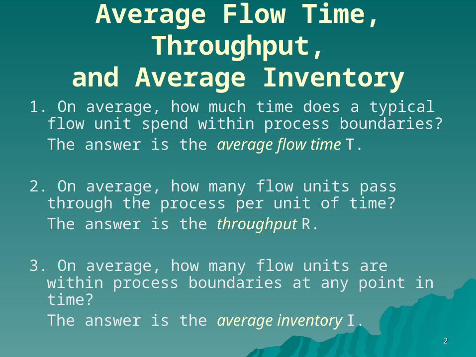
1. On average, how much time does a typical flow unit spend within process boundaries?
The answer is the average flow time T.
2. On average, how many flow units pass through the process per unit of time?
The answer is the throughput R.
3. On average, how many flow units are within process boundaries at any point in time?
The answer is the average inventory I.
33
Little's Law
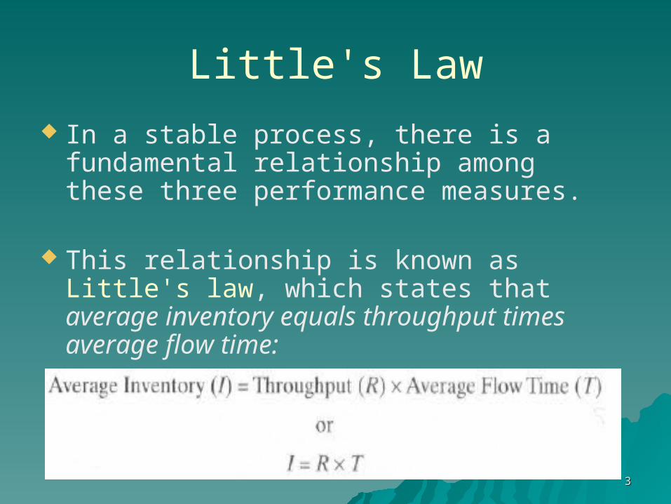
In a stable process, there is a fundamental relationship among these three performance measures.
This relationship is known as Little's law, which states that average inventory equals throughput times average flow time:
44
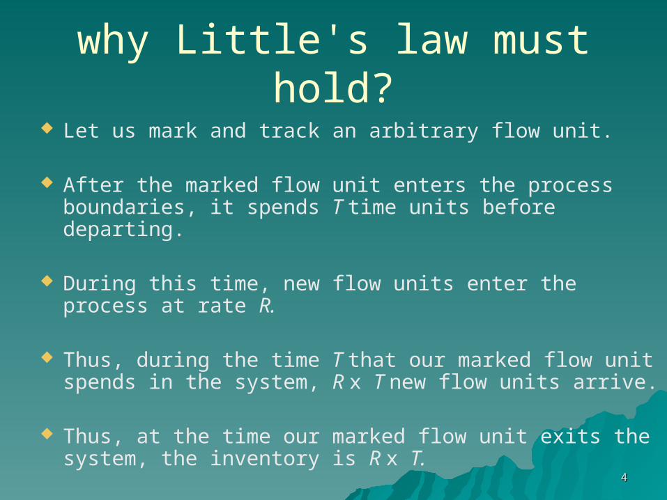
why Little's law must hold? Let us mark and track an arbitrary flow unit.
After the marked flow unit enters the process boundaries, it spends T time units before departing.
During this time, new flow units enter the process at rate R.
Thus, during the time T that our marked flow unit spends in the system, R x T new flow units arrive.
Thus, at the time our marked flow unit exits the system, the inventory is R x T.
55
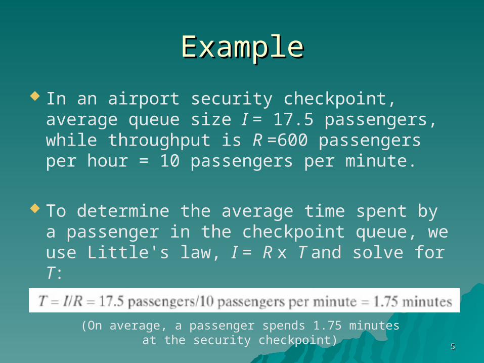
ExampleExample
In an airport security checkpoint, average queue size I = 17.5 passengers, while throughput is R =600 passengers per hour = 10 passengers per minute.
To determine the average time spent by a passenger in the checkpoint queue, we use Little's law, I = R x T and solve for T:
(On average, a passenger spends 1.75 minutes at the security checkpoint)
66
implications of Little's law
1. Of the three measures of performance, a process manager need only focus on two measures because they directly determine the third measure via Little's law.
2. For a given level of throughput in any process, the only way to reduce flow time is to reduce inventory and vice versa.
77
Material Flow
A fast-food restaurant processes an average of 5,000 kilograms (kg) of hamburgers per week.
Typical inventory of raw meat in cold storage is 2,500 kg.
The process in this case is the restaurant and the flow unit is a kilogram of meat.
88
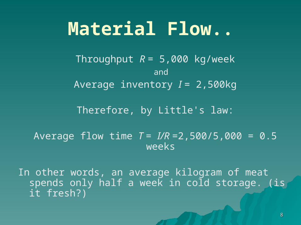
Material Flow..
Throughput R = 5,000 kg/week and
Average inventory I = 2,500kg
Therefore, by Little's law:
Average flow time T = I/R =2,500/5,000 = 0.5 weeks
In other words, an average kilogram of meat spends only half a week in cold storage. (is it fresh?)

99
Customer Flow The cafe Den Drippel in Ninove, Belgium, serves
on average 60 customers per night.
A typical night at Den Drippel is long, about 10 hours.
At any point in time, there are on average 18 customers in the cafe.
These customers are either enjoying their food and drinks, waiting to order, or waiting for their order to arrive.
1010
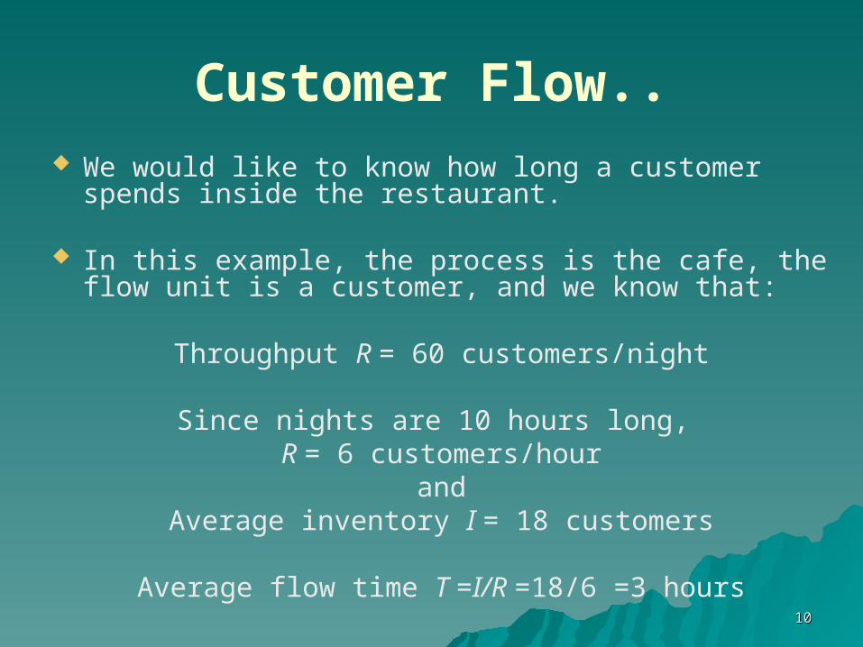
Customer Flow.. We would like to know how long a customer
spends inside the restaurant.
In this example, the process is the cafe, the flow unit is a customer, and we know that:
Throughput R = 60 customers/night
Since nights are 10 hours long, R = 6 customers/hour
andAverage inventory I = 18 customers
Average flow time T =I/R =18/6 =3 hours

1111
Job Flow A branch office of an insurance company
processes 10,000 claims per year.
Average processing time is three weeks.
We want to know how many claims are being processed at any given point.
Assume that the office works 50 weeks per year.
The process is a branch of the insurance company, and the flow unit is a claim.
1212
Job Flow..
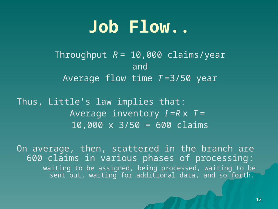
Throughput R = 10,000 claims/yearand
Average flow time T =3/50 year
Thus, Little's law implies that:Average inventory I =R x T = 10,000 x 3/50 = 600 claims
On average, then, scattered in the branch are 600 claims in various phases of processing:
waiting to be assigned, being processed, waiting to be sent out, waiting for additional data, and so forth.
1313
Cash Flow
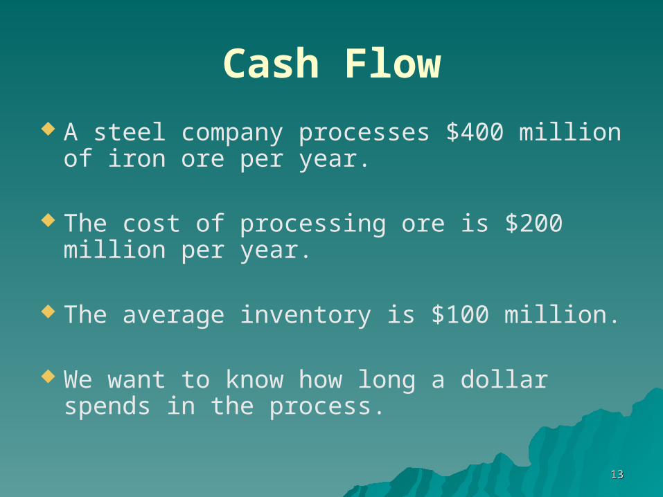
A steel company processes $400 million of iron ore per year.
The cost of processing ore is $200 million per year.
The average inventory is $100 million.
We want to know how long a dollar spends in the process.
1414
Cash Flow..
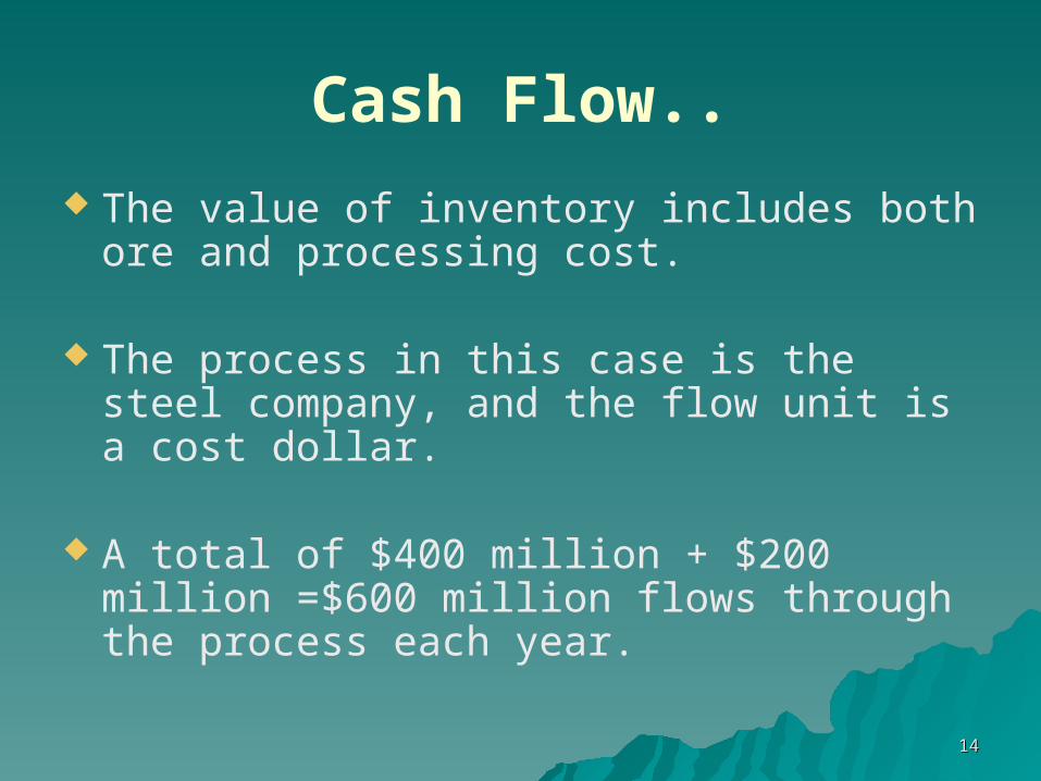
The value of inventory includes both ore and processing cost.
The process in this case is the steel company, and the flow unit is a cost dollar.
A total of $400 million + $200 million =$600 million flows through the process each year.
1515
Cash Flow..
Throughput R = $600million/yearand
Average inventory I =$100 million
We can thus deduce the following information:
Average flow time T =I/R =100/600 =1/6 year =2 months
On average, then, a dollar spends two months in the process.
1616
Cash Flow..
In other words, there is an average lag of two months between the time a dollar enters the process (in the form of either raw materials or processing cost) and the time it leaves (in the form of finished goods).
Thus, each dollar is tied up in working capital at the factory for an average of two months.
1717
Cash Flow (Accounts Receivable)
A major manufacturer sells $300 million worth of cellular equipment per year.
The average amount in accounts receivable is $45 million.
We want to determine how much time elapses from the time a customer is billed to the time payment is received.
In this case, the process is the manufacturer's accounts-receivable department, and the flow unit is a dollar.
1818
Cash Flow (Accounts Receivable)..
Throughput R = $300 million/yearand
Average inventory I =$45 million
Thus, Little's law implies thatAverage flow time T =1/R =45/300 year =0.15 years
=1.8 months
On average, 1.8 months elapse from the time a customer is billed to the time payment is received.
Any reduction in this time will result in revenues reaching the manufacturer more quickly.
1919
Service Flow (Financing Applications at Auto-Moto)
Auto-Moto Financial Services provides financing to qualified buyers of new cars and motorcycles.
Having just revamped its application-processing operations, Auto-Moto Financial Services is now evaluating the effect of its changes on service performance.
Auto-Moto receives about 1,000 loan applications per month and makes accept/reject decisions based on an extensive review of each application.
Assume a 3O-day working month.

2020
Financing Applications at Auto-Moto..
Until last year (we will call "Process I"), Auto-Moto Financial Services processed each application individually.
On average, 20% of all applications received approval.
An internal audit showed that, on average, Auto-Moto had about 500 applications in process at various stages of the approval/rejection procedure.
In response to customer complaints about the time taken to process each application, Auto-Moto called in Kellogg Consultants (KC) to help streamline its decision-making process.

2121
Financing Applications at Auto-Moto..
KC quickly identified a key problem with the current process:
– although most applications could be processed fairly quickly, some took a disproportionate amount of time because of insufficient or unclear documentation.
KC suggested the following changes to the process (we will call "Process II"):

2222
KC suggested the following changes:
1. Because the percentage of approved applications is fairly low, an Initial Review Team should be set up to preprocess all applications.
2. Each application would fall into one of three categories: A (looks excellent), B (needs more detailed evaluation), and C (reject summarily).
A and B applications would be forwarded to different specialist subgroups.
3. Each subgroup would then evaluate the applications in its domain and make accept/reject decisions.
2323
Financing Applications at Auto-Moto..
Process II was implemented on an experimental basis.
The company found that, on average, 25% of all applications were As, 25% Bs, and 50% Cs.
Typically, about 70% of all As and 10% of all Bs were approved on review. (Cs were rejected.)
Internal audit checks further revealed that, on average, 200 applications were with the Initial Review Team undergoing preprocessing.
Just 25, however, were with the Subgroup A Team undergoing the next stage of processing and about 150 with the Subgroup B Team.
2424
Financing Applications at Auto-Moto..
Auto-Moto Financial Services wants to determine whether the implemented changes have improved service performance.
Observe that the flow unit is a loan application.
On average, Auto-Moto Financial Services receives and processes 1,000 loan applications per month.
2525
Financing Applications at Auto-Moto..
Under Process I, we know the following:
Throughput R = 1,000 applications/monthand
Average inventory I =500 applications
Thus, we can conclude that:
Average flow time T =I/R
T = 500/1,000 months = 0.5 months = 15 days
(In Process I, each application spent on average 15 days with Auto-Moto before receiving an accept/reject decision.)
2626
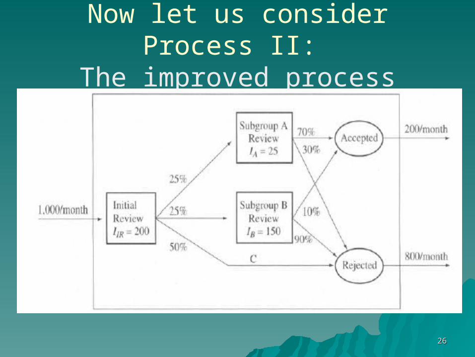
Now let us consider Process II: The improved process
2727
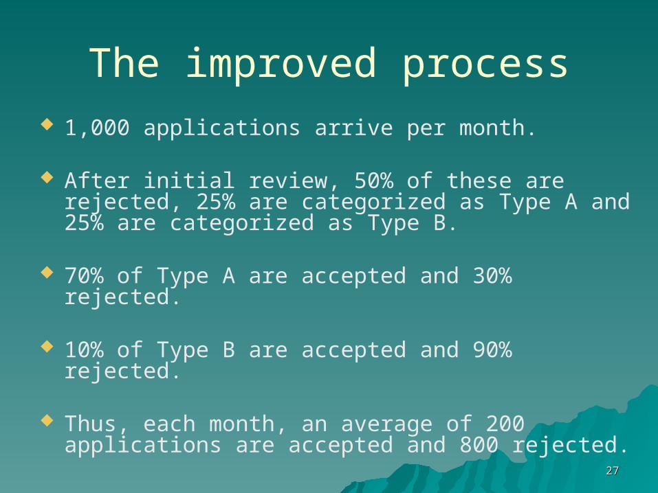
The improved process 1,000 applications arrive per month.
After initial review, 50% of these are rejected, 25% are categorized as Type A and 25% are categorized as Type B.
70% of Type A are accepted and 30% rejected.
10% of Type B are accepted and 90% rejected.
Thus, each month, an average of 200 applications are accepted and 800 rejected.

2828
The improved process.. Furthermore, on average, 200 applications
are with the Initial Review Team, 25 with the Subgroup A Team, and 150 with the Subgroup B Team.
Thus we can conclude that for Process II
Throughput R = 1,000 applications/monthand
Average inventory I = 200 + 150 + 25 = 375 applications
2929
The improved process..
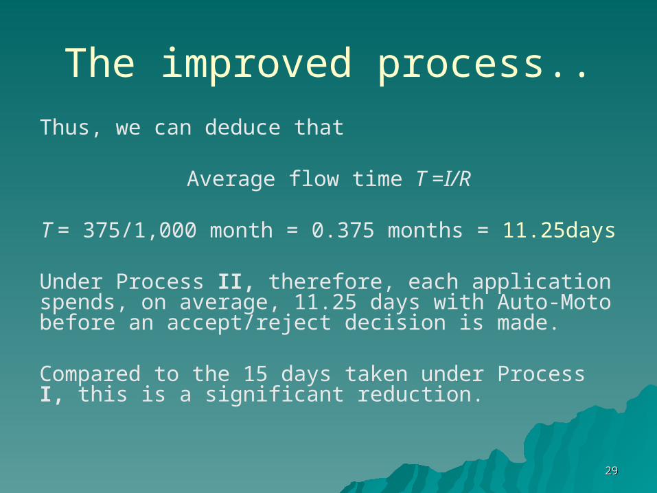
Thus, we can deduce that
Average flow time T =I/R
T = 375/1,000 month = 0.375 months = 11.25days
Under Process II, therefore, each application spends, on average, 11.25 days with Auto-Moto before an accept/reject decision is made.
Compared to the 15 days taken under Process I, this is a significant reduction.

3030
Analyzing Financial Flows through Financial Statements
MBPF Inc. manufactures prefabricated garages.
The manufacturing facility purchases sheet metal that is formed and assembled into finished products-garages.
Each garage needs a roof and a base.
We now consider MBPF Inc. and analyze its three financial statements: income statement, balance sheet, and the more detailed cost of goods sold (COGS) statement for 2004.
With an appropriate use of Little's law, this analysis will help us understand the current performance of the process.
3131
Analyzing Financial Flows through Financial Statements
In 2004, MBPF operations called for the purchase of both sheet metal (raw materials) and prefabricated bases (purchased parts).
Roofs were made in the fabrication area from sheet metal and then assembled with prefabricated bases in the assembly area.
Completed garages were stored in the finished goods warehouse until shipped to customers.
3232
Assessing Financial Flow Performance
Our objective is to study cash flows at MBPF in order to determine how long it takes for a cost dollar to be converted into recovered revenue.
For that, we need a picture of process-wide cash flows.
The flow unit here is a cost dollar, and the process is the entire factory, including the finished-goods warehouse.
3333
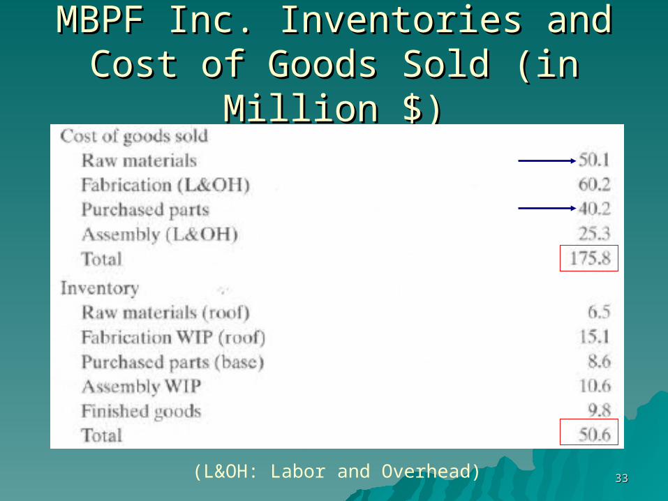
MBPF Inc. Inventories and Cost of MBPF Inc. Inventories and Cost of Goods SoldGoods Sold (in (in MillionMillion $) $)
(L&OH: Labor and Overhead)
3434
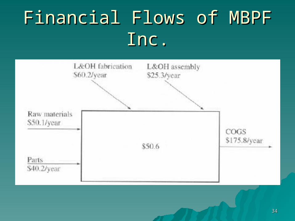
Financial Flows of MBPF Inc.Financial Flows of MBPF Inc.
3535
Assessing Financial Flow Performance..
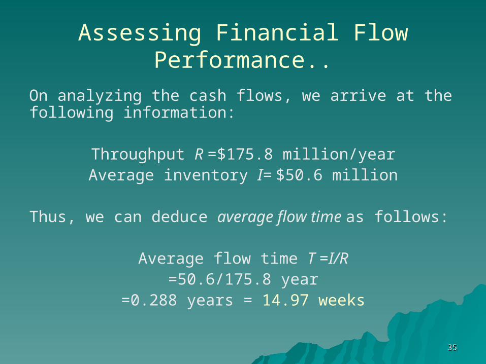
On analyzing the cash flows, we arrive at the following information:
Throughput R =$175.8 million/yearAverage inventory I= $50.6 million
Thus, we can deduce average flow time as follows:
Average flow time T =I/R=50.6/175.8 year
=0.288 years = 14.97 weeks

3636
Assessing Financial Flow Performance..
So the average dollar invested in the factory spends roughly 15 weeks before it leaves the process through the door of the finished-goods inventory warehouse.
In other words, it takes on average 14.97 weeks for a dollar invested in the factory to be billed to a customer.
3737
Assessing Financial Flow Performance..
A similar analysis can be performed for the accounts-receivable (AR) department.
Let us find out how long it takes, on average, between the time a dollar is billed to a customer (and enters AR) to the time it is collected as cash from the customer's payment.
3838
Assessing Financial Flow Performance..
In this case, process boundaries are defined by the AR department, and the flow unit is a dollar of accounts receivable.
For this part, we will use the income statement and the balance sheet for the MBPF Inc.
3939
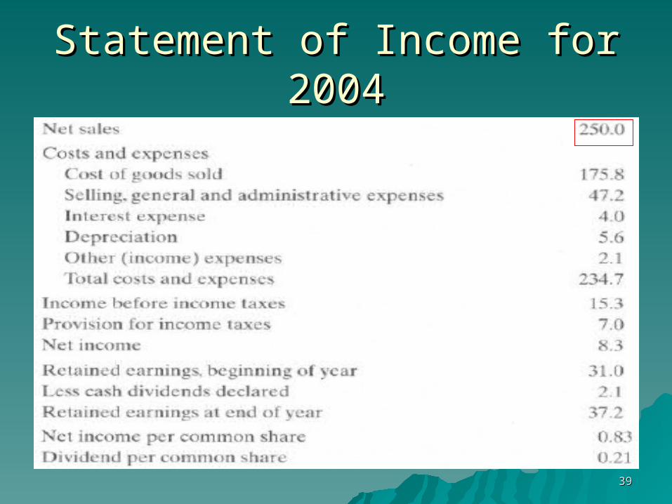
Statement of IncomeStatement of Income forfor 2004 2004
4040
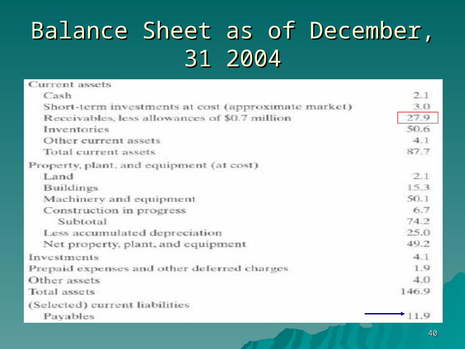
Balance Sheet as of December, 31 Balance Sheet as of December, 31 20042004
4141
Assessing Financial Flow Performance..
From Income Statement, note that MBPF has annual sales (and thus an annual flow rate through AR) of $250 million.
From Balance Sheet, note that accounts receivable total $27.9 million.
When we analyze flows through AR, we arrive at the following information:
4242
Assessing Financial Flow Performance..
Throughput RAR =$250 million/year [Net Sales]
Average inventory IAR =$27.9 million [Receivables]
Accordingly, the average flow time through AR is
Average flow time TAR =IAR / RAR
=27.9/250years=0.112 years =5.80 weeks
4343
Assessing Financial Flow Performance..
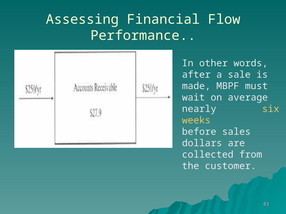
In other words, after a sale is made, MBPF must wait on average nearly six weeksbefore sales dollars are collected from the customer.
4444
Assessing Financial Flow Performance..
Finally, the same analysis can be done for the accounts-payable (AP)-or purchasing-process at MBPF Inc.
Recall that MBPF purchases both raw materials and parts.
Let us find out how long it takes; on average, between the time raw material or parts are received and the supplier bills MBPF (and the bill enters AP) to the time MBPF pays the supplier.
4545
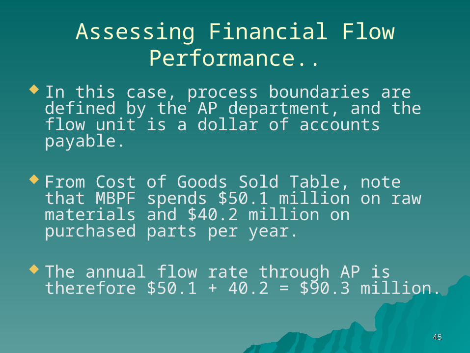
Assessing Financial Flow Performance..
In this case, process boundaries are defined by the AP department, and the flow unit is a dollar of accounts payable.
From Cost of Goods Sold Table, note that MBPF spends $50.1 million on raw materials and $40.2 million on purchased parts per year.
The annual flow rate through AP is therefore $50.1 + 40.2 = $90.3 million.

4646
Assessing Financial Flow Performance..
The balance sheet shows that the average inventory in purchasing (accounts payables) is $11.9 million.
Letting the subscript AP denote accounts payable, we can use Little's law to determine the average flow time through AP department:
TAP =IAP / RAP
= 11.9 / 90.3=0.13 years =6.9 weeks
In other words, it takes MBPF on average 6.9 weeks to pay a bill.

4747
Cash-to-Cash Cycle Performance
Overall, there is an average lag of about 21 weeks (15 weeks in production and 5.8 weeks in AR) between the point at which cost dollars are invested and the point at which sales dollars are received by MBPF.
We call this time of converting cost dollars into sales (21 weeks) the cost-to-cash cycle for this process.
Yet MBPF only pays for the cost dollars it invests in the form of purchased parts and raw materials after 6.9 weeks.
Its total "cash-to-cash" cycle therefore is21 - 6.9 =14.1 weeks
4848
Targeting Improvement with Detailed Financial Flow Analysis
To identify areas within the process that can benefit most from improvement, we need a more detailed flow analysis.
We now consider detailed operations by analyzing dollar flows separately through each of the following areas or departments of the process:– raw materials, purchased parts, fabrication, assembly,
and finished goods.
The flow unit in each case is a cost dollar.
4949
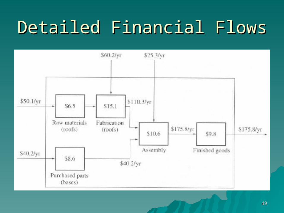
Detailed Financial FlowsDetailed Financial Flows
5050
Detailed Financial FlowsDetailed Financial Flows....
For each department, we obtain throughput by adding together the cost of inputs and any labor and overhead (L&OH) incurred in the department.
So, the throughput rate through fabrication is
$50.1 million/year in raw materials+ $(60.2million in labor and overhead
= $110.3 million/year

5151
Detailed Financial FlowsDetailed Financial Flows.... The throughput through the assembly area
is
$110.3 million/year in roofs
+ $40.2 million/year in bases
+ $25.3 million/year in labor and overhead
=$175.8 million/year
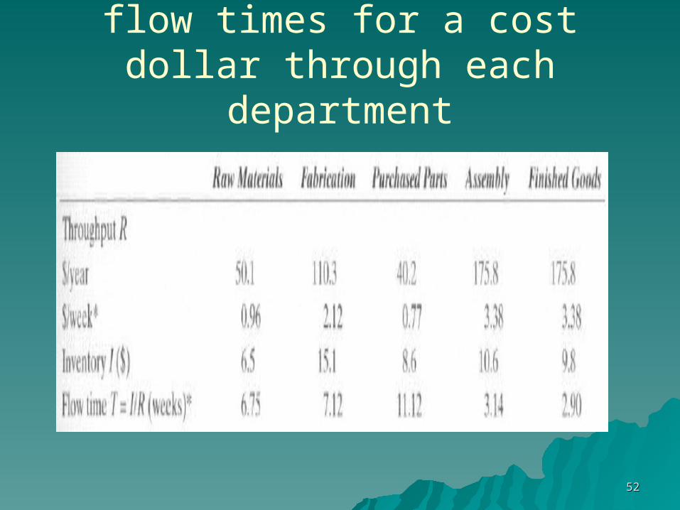
By analyzing the various flows through these four stages, we find the flow times for a cost dollar through each department.
5252
flow times for a cost dollar through each department
5353
Detailed Financial FlowsDetailed Financial Flows.... Working capital in each department includes the
amount of inventory in it.
Flow time in each department represents the amount of time a cost dollar spends, on average, in that department.
Reducing flow time, therefore, reduces MBPF's required working capital.
Knowing this principle, we are prompted to ask, In which department does a reduction of flow time have the greatest impact on working capital?
5454
Detailed Financial FlowsDetailed Financial Flows.... Because inventory equals the product of flow
time and throughput, the value of reducing flow time, say, by one week in any department is proportional to its throughput rate.
For example, because throughput through the finished-goods warehouse is $3.38 million per week, reducing flow time here by one week saves $3.38 million in working capital (inventory).
But because the throughput rate through purchased parts is only $0.77 million per week, a one-week reduction in flow time saves only $0.77 million in working capital.

5555
Detailed Financial FlowsDetailed Financial Flows....
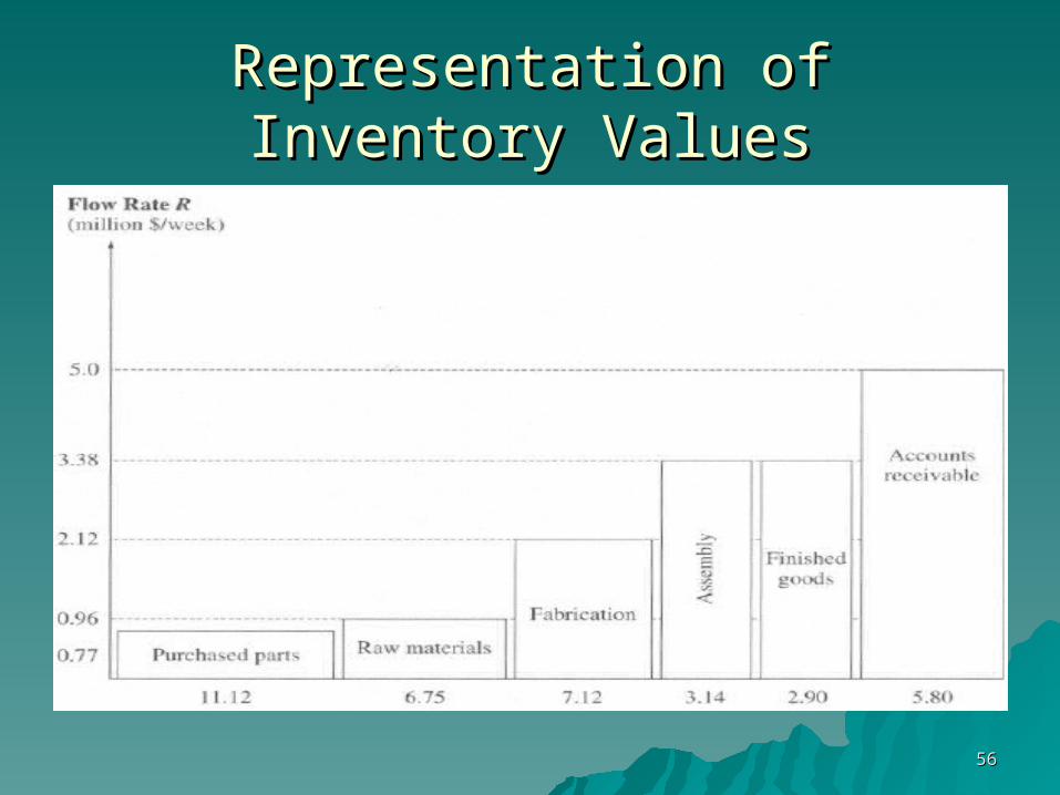
For each department, we plot throughput on the vertical axis and flow time on the horizontal axis.
Each department corresponds to a rectangle whose area represents the inventory in the department:
5656
Representation of Inventory ValuesRepresentation of Inventory Values
5757
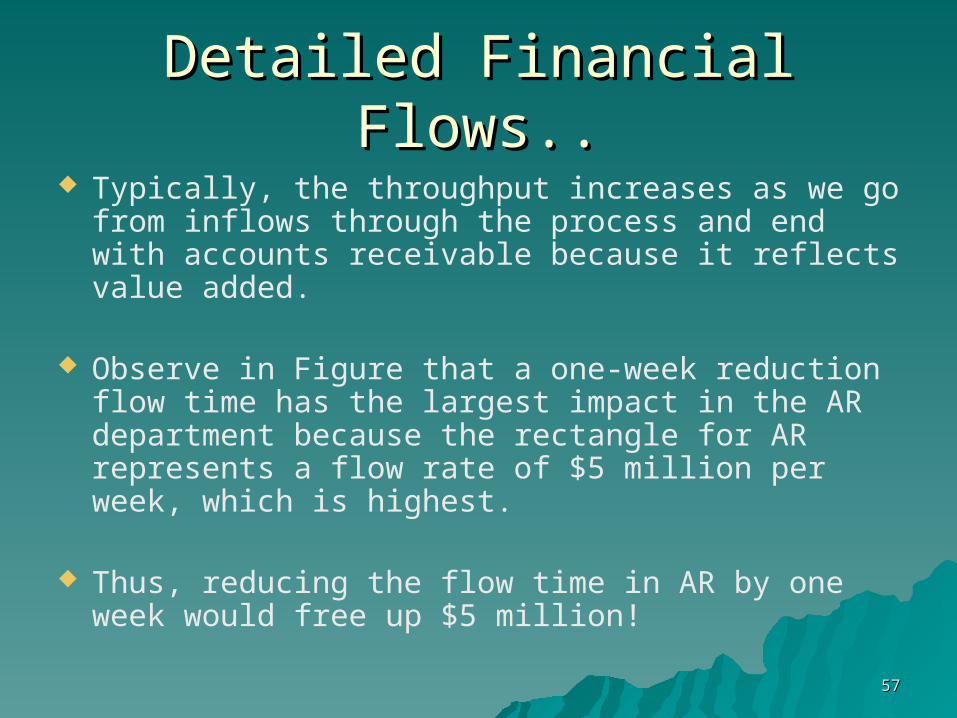
Detailed Financial FlowsDetailed Financial Flows.... Typically, the throughput increases as we go from
inflows through the process and end with accounts receivable because it reflects value added.
Observe in Figure that a one-week reduction flow time has the largest impact in the AR department because the rectangle for AR represents a flow rate of $5 million per week, which is highest.
Thus, reducing the flow time in AR by one week would free up $5 million!
5858
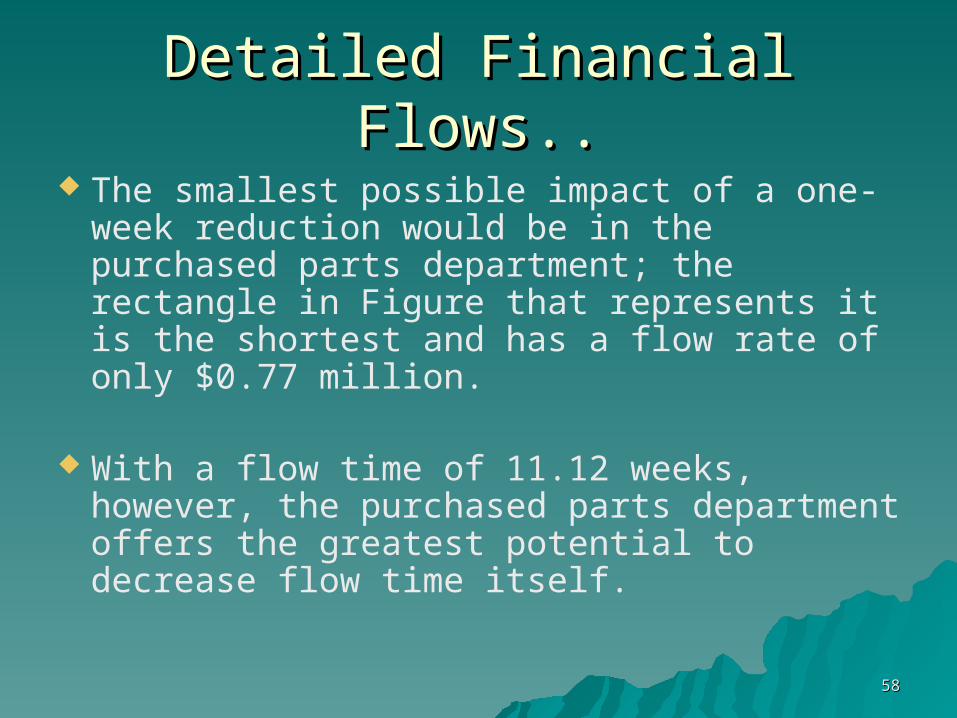
Detailed Financial FlowsDetailed Financial Flows....
The smallest possible impact of a one-week reduction would be in the purchased parts department; the rectangle in Figure that represents it is the shortest and has a flow rate of only $0.77 million.
With a flow time of 11.12 weeks, however, the purchased parts department offers the greatest potential to decrease flow time itself.
5959
Inventory Turns (Turnover Ratio)
In addition to the average level of inventory and the average flow time, practicing operations managers, accountants, and financial analysts often use the concept of inventory turns or turnover ratio to show how many times the inventory is sold and replaced during a specific period.
In the accounting literature, inventory turns is defined as the cost of goods sold divided by average inventory.
6060
Turnover Ratio..
The cost of goods sold during a given period is nothing other than throughput, expressed in monetary units.
Therefore, in our broader view of inventory, inventory turns, or turnover ratio, is defined as the ratio of throughput to average inventory.
Inventory turns =R / I

6161
Turnover Ratio..
But we can use Little's law, I = R x T, to come up with an equivalent definition of inventory turns as follows:
Inventory turns = R/I= R/(R x T)
(R cancels out)
=1 / T
6262
Turnover Ratio..
In other words, inventory turns is the reciprocal of average flow time and thus is a direct operational measure.
This directly shows why high turns are attractive: a company with high inventory turns has small flow times and thus is quicker at turning its inputs into sold outputs.

6363
Turnover Ratio.. To derive a meaningful turnover ratio, we
must specify the flow unit and measure inventory and throughput in the same units.
Some organizations measure turns as the ratio of sales to inventory.
This measure has a drawback in that sales (a measure of throughput) are expressed in sales dollars but inventory is measured in cost dollars.
6464
Turnover Ratio..
A better way to calculate turns is the ratio of cost of goods sold (COGS)- labor, materials,
and overhead expenses allocated to the products- to inventory because both are measured in cost dollars.
Measuring turns as the ratio of sales to inventory can lead to erroneous conclusions when measuring process performance.
6565
Example
Let us return to the MBPF financial statements to analyze inventory turns.
We will use cost dollar as the flow unit and designate the factory and the finished-goods warehouse as the process:
Turns =Throughput/Inventory= ($175.8/year) / $50.6 = 3.47/year
In other words, during one year MBPF Inc. sells and thus replenishes its average inventory aboutthree times.