1  

The Real Effects of Liquidity During the Financial Crisis: Evidence

from Automobiles1

Efraim Benmelech Ralf R. Meisenzahl Rodney Ramcharan Northwestern University Federal Reserve Board Federal Reserve Board

and NBER

October 2014

Abstract

This paper shows that illiquidity in short-term credit markets during the financial crisis may have

sharply curtailed the supply of non-bank consumer credit. Using a new data set linking every car

sold in the United States to the credit supplier involved in each transaction, we show that the

collapse of the asset-backed commercial paper market decimated the financing capacity of

captive leasing companies in the automobile industry. As a result, car sales in counties that

traditionally depended on captive-leasing companies declined sharply. Although other lenders

increased their supply of credit, the net aggregate effect of illiquidity on car sales is large and

negative. We conclude that the decline in auto sales during the financial crisis was caused in part

by a credit supply shock driven by the illiquidity of the most important providers of consumer

finance in the auto loan market: the captive leasing arms of auto manufacturing companies.

These results also imply that interventions aimed at arresting illiquidity in credit markets and

supporting the automobile industry might have helped to contain the real effects of the crisis.

                                                                                                                         1 We thank Gadi Barlevi, Dan Covitz, Diana Hancock, Arvind Krishnamurthy, Gregor Matvos, Jonathan Parker, Wayne Passmore, Karen Pence, Phillip Schnabl, Andrei Shleifer, Jeremy Stein and seminar participants at the Basel Research Task Force, Dutch National Bank, Federal Reserve Board, Federal Reserve Bank of Chicago, Indiana University (Kelley School of Business), NBER Summer Institute, and Pennsylvania State University (Smeal) for very helpful comments. Della Cummings, Sam Houskeeper, Jeremy Oldfather, and Jeremy Trubnick provided excellent research assistance. Benmelech is grateful for financial support from the National Science Foundation under CAREER award SES-0847392. The views expressed here are those of the authors and do not necessarily reflect the views of the Board of Governors or the staff of the Federal Reserve System.

2  

1. Introduction

Financial crises can have large adverse effects on real economic activity. Illiquidity in one corner

of the financial system and large realized balance-sheet losses in the financial sector can lead to a

contraction in the aggregate supply of credit and a decline in economic activity.2 Consistent with

these theoretical predictions, there is growing evidence from the 2007–2009 financial crisis that

the balance-sheet losses incurred by traditional financial institutions—banks and credit unions—

may have led to a fundamental post-crisis disruption in credit intermediation, contributing to the

recession and the slow economic recovery (Ramcharan et al., 2013, forthcoming; Chodorow-

Reich, 2014).3

However, non-bank financial institutions— such as finance and leasing companies—

have historically been important sources of credit, especially for consumer durable goods

purchases such as automobiles and appliances (Ludvigson, 1998). For example, non-bank

institutions accounted for more than a half of all new cars bought in the United States before the

crisis. Unlike most traditional banks, non-bank financial institutions are more closely connected

to the shadow banking system, relying primarily on short-term funding markets, such as the

asset-backed commercial paper (ABCP) market, for funding.

We investigate how runs in the ABCP market and the loss of financing capacity at non-

bank institutions, such as the captive leasing arms of auto manufacturers, might have curtailed

the supply of auto credit, led to the collapse in car sales, and exacerbated the financial difficulties

of companies such as GM and Chrysler that were already on the verge of bankruptcy. Between

2007 and 2008, short-term funding markets in the United States came to a halt, as money market

funds (MMFs) and other traditional buyers of short-term debt fled these markets (Covitz, Liang,

and Suarez, 2013). Although the initial decline in 2007 was driven mainly by ABCP backed by

mortgage-backed securities, the decline following the Lehman Brothers bankruptcy affected all

ABCP issuers.

                                                                                                                         2 See, e.g., Allen and Gale (2000), Diamond and Rajan (2005, 2011), Shleifer and Vishny (2010). 3 The crisis may have also disrupted intermediation even at non-traditional lenders like internet banks (Ramcharan

and Crowe, 2012).

3  

By early 2009, growing illiquidity in the ABCP market—one of the major sources of

short-term credit in the United States—made it difficult for many non-bank intermediaries to roll

over debt or secure new funding (Campbell et al., 2011). This illiquidity in short-term funding

markets coincided with the collapse of several large non-bank lenders. Chief among these

lenders was the General Motors Acceptance Corporation (GMAC)—the financing arm of

General Motors (GM) and one of the largest providers of auto financing in the world. At the

same time, automobile sales fell dramatically in 2008 and 2009, and GM and Chrysler eventually

filed for Chapter 11 bankruptcy protection.

In order to better understand the economic consequences of these disruptions in short-

term funding markets, we use a proprietary microlevel data set that includes all new car sales in

the United States. Our data set matches every new car to the sources of financing used in the

transaction (for example, auto loan or lease) and identifies the financial institution involved in

the transaction. The data, which are reported quarterly starting in 2002, also identify the county

in which the car was registered, along with the car’s make and model. This microlevel detailed

information and the spatial nature of the data enable us to develop an empirical identification

strategy that can help identify how captives’ loss of financing capacity might have affected car

sales in the United States.

Our identification strategy hinges on the notion that by the end of 2008, liquidity runs in

the ABCP market and the dislocations in other short-term funding markets had decimated the

financing capacity of the captive financing arms of automakers. We then show cross-sectionally

that in counties that are historically more dependent on these captive arms for auto credit, sales

financed by captive lessors fell dramatically in 2009. In particular, a one standard deviation

increase in a county’s dependence on captive financing before the crisis is associated with a 10%

drop in sales financed by captive lessors after the second quarter of 2009.

Next, we show that our results are driven by a liquidity shortage in short-term credit

markets, supplementing our cross-sectional evidence with panel regressions by adding a time-

series dimension to our analysis. Money market funds were the main purchasers of ABCP,

holding about 40% of commercial paper in mid-2007.4 The bankruptcy of Lehman Brothers on

                                                                                                                         4 Pozsar et al. (2010) survey the shadow banking system and highlight the crucial role that MMFs play for short-

term credit and securitization.

4  

September 15, 2008 triggered heavy outflows from MMFs and was a leading factor in the

evaporation of liquidity in the commercial paper market.5 Captive financing entities relied

predominantly on MMFs to finance their commercial paper issuances. We argue that the collapse

of the commercial paper market significantly reduced the funding available for leasing

companies to finance their operations.

Consistent with this hypothesis, we find that the number of retail car sales financed by

captive leasing arms declined as aggregate flows into MMFs dried up. The decline in auto sales

was exacerbated in counties that are historically more dependent on captive lease financing.

During a quarter when the growth in flows in MMFs was at the 25th percentile, a one standard

deviation increase in captive dependency is associated with a 3% drop in captive sales growth.

However, with the growth in flows into MMFs at the 75th percentile, a similar increase in

captive dependence is associated with only a 0.3% drop in captive sales growth.

Whereas we find that captive leasing arms reduced credit supply to potential car buyers,

we also find evidence for substitution in that sales financed by noncaptive lenders—those

financial institutions more dependent on traditional deposits for funding—actually rose during

this period in counties with higher dependency on captive financing. The evidence on

substitution from captive leasing to other forms of financing suggests that our results are driven

not by latent demand factors but rather by a credit supply shock. However, even with the

substitution to other lenders, the aggregate effects of disruptions in the short-term credit markets

on auto sales appear large. We find that regardless of the source of financing, aggregate car sales

dropped more sharply after the second quarter of 2009 in counties that depend more on captive

financing.

Next, the richness of our data and, in particular, the availability of make-level data allow

us to alleviate county-level omitted variables concerns. More specifically, we use a different

aggregation of the data in which the unit of observation is at the make-county level for the four

largest automakers: Toyota, GM, Ford, and Honda. The make-county data aggregation enables

us to control for county fixed effects as well as make fixed effects in our regression analysis. We

find that the impact of captive dependence on captive financed sales remains negative and

                                                                                                                         5 The day after Lehman’s failure, the Reserve Primary Fund, a $62 billion MMF, announced that it had “broken the

buck” (its share price had fallen below $1) because of losses on Lehman debt.

5  

statistically significant at the 1% level after controlling for both county and make fixed effects.

The level of detail in the dataset also allows us to exploit the segmentation in car markets

within makes and across models to further address these omitted variables concerns. Car makers

use different models to appeal to different types of consumers at different price points. GM for

example, markets Chevrolet towards nonluxury buyers, while Cadillac is aimed at wealthier

consumers. We can thus use county-model fixed effects to non-parametrically control for

differences in demand within a county across different model segments. Our results remain

unchanged.

Last, we use some of the attempts to regulate the financial system after the crisis to

identify further how the supply of short-term funding might shape car sales. Notably, large banks

incurred sizable losses due to their ABCP conduits. Financial regulation after the crisis also

drastically curtailed banks’ ability to use short-term funding markets to fund their activities. In

contrast, nonbank financial institutions, such as captive financiers, faced fewer barriers to

operating in these markets. We find that after these regulatory changes, captive lessors may have

garnered a sizable competitive advantage relative to large banks in retail automobile lending. All

this suggests that financial regulation after the crisis might have pushed a greater share of

intermediation into the shadow banking system.

Taken together, these results imply that funding disruptions in the short-term credit

markets during the recent financial crisis had a significant negative impact on car sales. This

evidence of a credit supply shock adds to our understanding of financial crises more broadly, and

complements those papers that emphasize alternative mechanisms, such as the role of debt and

deleveraging, that might shape post–credit boom economies (see Mian and Sufi, 2010, 2014a;

Mian, Rao and Sufi, 2013; Rajan and Ramcharan, forthcoming). We argue that a credit supply

channel was in particular important in the new car auto market during the crisis since more than

80% of new cars in the U.S. are financed by captive leases and auto loans from leasing

companies and other financial institutions, and only less than 20% are bought for in all cash

transactions.

Our evidence also tentatively suggests that the various Treasury and Federal Reserve

programs aimed at arresting illiquidity in credit markets and supporting the automobile industry

might have helped to contain the real effects of the crisis.

6  

Our paper also adds to the broader literature on the effects of financial markets and bank

lending on real economic outcomes.6 But whereas previous studies of the financial crisis

document the importance of short-term funding for banks’ liquidity and lending, less is known

about the real consequences of the collapse of short-term funding markets. Also less well

understood is the importance of leasing companies in the provision of credit in auto markets and

how these institutions might be connected to nontraditional sources of financing. We fill this

void by documenting that the collapse of short-term funding reduced auto lending by financial

institutions, which in turn resulted in fewer purchases of cars and reduced economic activity. We

also provide evidence that illiquidity in the short-term funding markets may have played an

important role in limiting the supply of non-bank consumer credit during the crisis, as the

collapse of the ABCP market decimated the financing capacity of many captive financing

companies.

The rest of the paper is organized as follows. Section 2 describes the institutional

background of captives’ ABCP funding and the data. We discuss identification concerns in

Section 3. Section 4 provides text evidence from the financial reports of auto dealerships on the

decline of credit by captive lessors. Section 5 discusses the data and the main summary statistics.

Sections 6, 7 and 8 present the results from our regression analyses. Section 9 concludes.

2. Captive leasing and asset-backed commercial paper

Most new cars in the United States are bought on credit through either car loans or leasing. Auto

credit peaked in 2006 at $785 billion, accounting for 32% of consumer debt. As Table 1

illustrates, although banks play an important role in automobile financing, about half of

automotive credit in 2005 came from finance companies, mostly captive lessors—leasing

companies set up by automakers to finance their own cars. One prominent captive lessor, for

example, was General Motors Acceptance Corp (GMAC), the captive leasing arm of General

Motors (GM), which provided credit to buyers of GM cars often at the point of sale through

financing arrangements with GM car dealerships.

                                                                                                                         6 See Acharya, Schnabl, and Suarez (2011); Ivanshina and Scharfstein (2010); Brunnermeier (2009); Gorton

(2010); Gorton and Metrick (2012); Khwaja and Mian (2008); Cornett et al. (2011); and Acharya and Mora (2013).

7  

Captive finance companies have long been central to automotive sales in the United

States. As manufacturers sought to popularize the automobile in the 1910s, they realized that the

automobile, with its unique combination of high cost, mass appeal, and independent dealership

networks, required a new form of financing in order to expand distribution and sales.

Commercial banks, however, were reluctant to use cars as collateral. Cars were still a relatively

novel and difficult to value durable good, and outsiders such as commercial banks had less

information about their depreciation path, especially given that the introduction of new models

often led to a sharp drop in the resale value of outgoing models. As a result, interest rates on car

loans were often close to the maximum legally allowed. Some bankers also thought it unwise for

commercial banks to provide credit for a luxury good, in part because of moral concerns that

credit for luxury goods may discourage thrift (Phelps, 1952). Car sales were also highly seasonal,

and the reluctance of banks to provide automotive financing also affected the ability of dealers to

finance their inventories (Hyman, 2011).

The organizational form of captives helped address some of these frictions. Captives such

as GMAC, which was founded in 1919, were vertically integrated into the manufacturer and

better able to overcome informational frictions surrounding the value of collateral; they knew,

for example, the model release schedule well ahead of arms-length lenders.7 Vertically integrated

captives were also less encumbered by moral objections to consumer spending, especially on

cars.8 Captive credit, by providing medium or long-term credit to consumers to pay for car

purchases, allowed dealers to receive cash on the sale of a car to a consumer. In some cases

dealers were also allowed to intermediate captive credit and earn additional markups. Also, by

providing floorplan financing, a form of credit collateralized by the dealer’s auto inventory,

                                                                                                                         7 Murfin and Pratt (2014) expand on these ideas within a theoretical model and provide evidence based on machine

equipment. 8 These points are echoed by William C. Durant in announcing the formation of GMAC in a letter dated March 15,

1919: “The magnitude of the business has presented new problems in financing which the present banking facilities

seem not to be elastic enough to overcome. . . . This fact leads us to the conclusion that the General Motors

Corporation should lend its help to solve these problems. Hence the creation of General Motors Acceptance

Corporation; and the function of that Company will be to supplement the local sources of accommodation to such

extent as may be necessary to permit the fullest development of our dealers’ business” (cited in Sloan, 1964, p. 303).

8  

captive credit relaxed financial constraints at the dealership level, enabling the automobile

manufacturer to receive cash on the sale of a car to the dealer.

Branch banking deregulation in the 1980s and early 1990s increasingly allowed banks to

operate nationally and to enter into new markets, including those previously dominated by

captives. However, the rise of securitization, which was in part a response to new bank capital

regulation, offered captive lessors new ways to tap into cheap funding and maintain their auto-

lending business in the face of new competition (Calder, 1992; Hyman, 2011).

Indeed, asset-backed commercial paper (ABCP) became the main source of funding for

captive lessors before the financial crisis. Table 2, based on non-public data collected by the

Federal Reserve, demonstrates the importance of commercial paper as a source of funding for

selected major automobile captives active in the United States. Given the nature of the data, we

cannot disclose the identities of the captive lessors in the table and instead label them Captive 1

through Captive 4. As Table 2 shows, commercial paper was a major source of funding for three

out of the four captive lessors. Although commercial paper accounted for just 10.2% of one

lessor’s liabilities (Captive 3), the other three captive lessors relied much more heavily on this

form of short-term funding, with the share of commercial paper in their liabilities ranging from

45.9% (Captive 2) to 75.12% (Captive 4).

A key advantage of ABCP funding is that it enables captive lessors to turn relatively

illiquid auto term loans into liquid assets that can be used to obtain funding for new loans. This is

done by pooling auto loans together and placing them in a special purpose vehicle (SPV) that is

bankruptcy remote from the originating captive lessor. The SPV in turn, issues short-term

secured commercial paper (ABCP) to finance loans and markets the commercial paper—

generally with a duration of no more than three months.9

Money market funds and other institutional investors seeking to invest in liquid and high-

yield short-term assets are the main buyers of commercial paper, and in mid-2007, just before the

turbulence in credit markets, MMFs held about 40% of outstanding commercial paper in the

United States. The bankruptcy of Lehman Brothers on September 15, 2008 and the “breaking of

the buck” at Reserve Primary Fund the next day triggered heavy outflows from MMFs, leading

the Treasury to announce an unprecedented guarantee program for virtually all MMF shares. The

                                                                                                                         9 For a detailed discussion of ABCP structures, see Acharya, Schnabl, and Suarez (2011).

9  

Federal Reserve followed suit by announcing a program to finance purchases of ABCP—which

were highly illiquid at the time—from MMFs. Despite these interventions, however, flows into

MMF remained highly erratic, and MMFs significantly retrenched their commercial paper

holdings. In the three weeks following Lehman’s bankruptcy, prime MMFs reduced their

holdings of commercial paper by $202 billion, a steep decline of 29%.

The reduction in commercial paper held by MMFs accounted for a substantial portion of

the decline in outstanding commercial paper during this period and contributed to a sharp rise in

borrowing costs for issuers of commercial paper. ABCP issuances also fell sharply amid the

turmoil in short-term credit markets, and the sharp outflows of assets from MMFs in the third

quarter of 2008 precipitated a run on many of these auto-related securitization pools. Figure 1

displays the outstanding amount of ABCP issued by SPVs associated with the captive leasing

arms of the big three American automakers: GMAC, Chrysler Financial (CF), and Ford Motor

Credit (FMC). Although the ABCP market began to weaken in 2007, automakers’ issuance of

ABCP began to collapse in the third quarter of 2008. Together, the big three captive lessors had

about $40 billion worth of ABCP outstanding in 2006 before they largely collapsed by the end of

2009.10

3. The endogeneity concern

3.1. The endogeneity concern

We hypothesize that the decline in auto sales was caused in part by a credit supply shock driven

by the illiquidity of captive lessors—the most important providers of consumer finance in the

auto loan market. That is, we argue that runs in the ABCP market and the loss of financing

capacity at the captive arms of the automakers curtailed the supply of auto credit, which in turn

caused a drop in car sales. To identify the credit supply channel, we construct a measure of a                                                                                                                          10 Ford’s financing arm, FMC, survived the crisis in part because of its continued access to the Federal Reserve’s

Commercial Paper Funding Facility (CPFF), which bought ABCP to alleviate liquidity pressures in the funding

markets after the Lehman collapse. The Federal Reserve announced the CPFF to provide a liquidity backstop for US

commercial paper issuers with high short-term credit ratings on October 14, 2008. Before losing access in January

2009, GMAC heavily relied on CPFF, selling a total of $13.5 billion ABCP to the facility. In contrast to GMAC and

CF, FMC was able to maintain its short-term credit rating and never lost access to CPFF, from which it had raised

almost $16 billion by summer 2009 and then began again to raise funds from private investors.

10  

county’s dependence on captive financing, defined as the ratio of the number of retail auto sales

financed by captives to the number of all retail auto sales. We then estimate the relation between

captive dependence and auto sales at the county level, controlling for the factors most likely to

affect the demand for automotive credit in the county.

However, identifying a credit supply channel using a regression of auto sales on a

measure of captive leasing is difficult because reliance on captive leasing is potentially

correlated with underlying demand side factors. For example, one can argue that the demand for

consumer credit from borrowers who rely on captive leasing may have fallen, too, since captive

lessors are often seen as providers of credit to riskier borrowers (Barron, Chong, and Staten,

2008; Einav, Jenkins, and Levin, 2013).11 And since some of these borrowers were also hit by

the housing crisis, it is possible that the dramatic fall in car sales in 2009 might have also been

driven by a demand shock.

3.2. Are our results driven by consumer demand?

Although the concern that auto sales financed by captive lessors plummeted because of lower

demand by risky borrowers is a valid one, three pieces of evidence suggest that a credit supply

shock was indeed an important factor in the decline of auto sales.

First, it is important to note that by the first quarter of 2007 only 15% of GMAC’s US-

serviced consumer asset portfolio was considered nonprime.12 That is, the vast majority of those

who relied on captive leasing were safer borrowers who had lower sensitivity to the housing

cycle.

Second, a demand-side shock should lead to an overall decline in all types of credit

regardless of the lender’s identity. In contrast, we find that although lending by captive lessors

fell dramatically during the crisis, sales financed by banks actually rose during this period—

although not enough to offset the decline. We argue that it is hard to reconcile the declining

                                                                                                                         11 Charles, Hurst, and Stephens (2010) document that minorities, in particular African Americans, are more likely to

receive auto loans from financing companies and pay, on average, higher interest rates on those loans. One plausible

explanation for this pattern is that minorities have, on average, lower credit scores and therefore are more likely to

receive financing from captives. For a detailed analysis of subprime aut0-lending contracts, see Adams, Einav, and

Levin (2009) and Einav, Jenkins, and Levin (2012). 12 See GMAC LLC, 8-K, April 26, 2007, File No. 001-03754.

11  

demand conjecture with the observed shift from captive leasing to bank financing during the

crisis. The substitution from captive leasing to banks is well illustrated in Panel (B) of Table 1.

The auto loan market share of finance companies—mostly captive lessors—was 51.3% in 2005

and declined to just 41.3% and 36.7% in 2009 and 2010, respectively. In contrast, the auto loan

market share of banks, including both credit unions and commercial banks rose from 44.9% in

2005 to 56.2% and 61.1% in 2009 and 2010, respectively.

Third, though captive lessors are key players in the provision of consumer credit, they are

also an important source of credit to auto dealerships. In particular, captive lessors provide

floorplan financing—a form of credit collateralized by the dealer’s auto inventory—that enable

dealerships to purchase their car inventory. Although it is not easy to obtain dealership-level data

on floorplan loans, we have read the financial reports of the largest publicly traded automotive

dealerships in the United States to understand the challenges that auto dealerships faced during

the great recession. In reading these reports we came across many instances in which these

companies list lack of financing for both consumers and dealerships as a first-order reason for

the decline in auto sales. That is, the illiquidity of captive lessors led to a decline in auto sales

through a credit supply channel that affected not only consumers but also car dealerships.

Nevertheless, to alleviate concerns about the endogeneity of captured leasing, we use

several identification strategies. We saturate our baseline specification with a battery of

economic and demographic characteristics that have been used in the literature to measure the

impact of housing and leverage on local demand. We also use the richness of the data to

nonparametrically control for demand within counties. We include placebo tests based on auto

cash sales as well as consumer expenditures on other goods and services, and we use the timing

of MMF flows to measure how temporal variation in the financing capacity of captives might

affect local sales. But before turning to the data and empirics, we first provide narrative-based

evidence on the decline in captive financing.

4. The decline in credit supply by captive lessors: evidence from auto dealership companies

Before we move to the statistical analysis, we present narratives from the Form 10-Ks of the

largest publicly traded dealership companies in the United States based on our reading of these

10Ks from 2006 to 2011. We collect and reproduce here those discussions that pertain to the role

12  

of captive leasing in the automotive industry in general and during the financial crisis in

particular.

4.1. AutoNation

By the end of 2006, AutoNation was the largest automotive retailer in the United States, owning

and operating 331 new vehicle franchises out of 257 stores located in major metropolitan

markets. AutoNation stores sold 37 different brands of new vehicles, primarily those

manufactured by Ford, General Motors, DaimlerChrysler, Toyota, Nissan, Honda, and BMW.

According to AutoNation' 2006 10K, the firm retailed approximately 600,000 new and used

vehicles through their stores.

In 2006, AutoNation relied heavily on floorplan borrowing from captive lessors, with a

total vehicle floorplan payable of $2,264.9 million, accounting for 74.7% of the company’s

current liabilities and 46.3% of its total liabilities. Similarly, in 2007, total vehicle floorplan was

$2,181.8 million, accounting for 75.2% of current liabilities and 43.6% of total liabilities. Indeed,

the importance of financing supplied by captive lessors for AutoNation as well as for its

customers is echoed in their 2009 Form 10-K:

We obtain a significant amount of financing for our customers through the captive

finance companies of automotive manufacturers, which companies were adversely

impacted by the turbulence in the capital markets as well as the overall economic

conditions in the United States. These conditions also adversely impacted other finance

companies, including GMAC, which received extensive federal support and is now

majority-owned by the U.S. Treasury. In 2009, the availability of automotive loans and

leases through many of these finance companies declined significantly, forcing us to

seek, at times unsuccessfully, alternative financing sources for our customers. We also

rely on the captive finance companies of automotive manufacturers for floorplan

financing to purchase new vehicle inventory. In 2009, many of these captive finance

companies altered their floorplan financing programs to our detriment, providing

additional restrictions on lending and increasing interest rates.13

                                                                                                                         13 AutoNation Form 10-K for the fiscal year ending December 31, 2009, pp. 22–23.

13  

4.2. Lithia Motors

Another large auto dealership company that is highly dependent on floorplan financing from

captive lessors is Lithia Motors, a NYSE publicly listed company. Operating in both new and

used vehicles markets, in 2006 Lithia Motors offered 30 brands of new vehicles through 193

franchises in the western United States, with DaimlerChrysler, General Motors, Toyota, and Ford

accounting for 41.0%, 19.4%, 10.9% and 7.3% of new vehicle sales, respectively. In its Form

10-K for the fiscal year ending in December 31, 2008 the company reports:

During 2008, overall macroeconomic issues have reduced consumers’ desire and

ability to purchase automobiles. An additional factor negatively impacting auto sales

has been a reduction in available options for consumer auto loans. The manufacturers’

captive financing companies have suffered additional pressure as the financial crisis

has raised their cost of funds and reduced their access to capital. This and financial

stress on manufacturers has prevented them from offering as many incentives designed

to drive sales, such as subsidized interest rates and the amount of loan to value they are

willing to advance on vehicles.14

The tightening of the credit markets experienced in 2008 reduced the number of loans

originated, restricted loans to more credit-worthy customers, reduced vehicle leasing

programs and increased the overall cost of financing.15

Lithia Motors again expresses concerns about tightening credit markets and their effects on both

dealerships and customers in its 2009 annual report:

Credit markets continued to remain tight in 2009. . . . These constraints in financing

resulted in fewer consumers in the market and less floor traffic at our stores. The

financial crisis has increased the cost of funds and reduced the access to capital for

                                                                                                                         14 Lithia Motors Form 10-K for the fiscal year ending December 31, 2008, p. 4. 15 Lithia Motors Form 10-K for the fiscal year ending December 31, 2008, p. 11.

14  

finance companies (including manufacturers’ captive finance companies).16

A lack of available credit continued to prove challenging to prospective purchasers of

our stores. One of the primary problems was the lack of vehicle inventory floorplan

financing, which is a basic requirement of the franchise agreement. Even for

prospective purchasers with existing floorplan financing, obtaining mortgage financing

on dealership real estate or committing to other significant capital investment proved

exceedingly difficult.17

As these reports reveal, access to finance was a major concern in the US auto market in 2008 and

2009. Lack of financing posed a problem not only to consumers but also to large, publicly traded

firms that relied heavily on floorplan financing from auto manufacturers’ leasing companies.

This widespread lack of credit was also listed as a key motivation for federal support of the

automobile sector.18 We turn now to the data and our empirical tests.

5. Data and summary statistics

We use a proprietary data set from R. L. Polk & Company (Polk) that records all new car

sales in the United States. Beginning in 2002, for each new car purchased in the United States,

the data set identifies vehicle make and model, such as Ford (make) Focus (model) or Toyota

(make) Camry (model), and whether the car was purchased by a private consumer (a retail

purchase), a firm (commercial purchase), or by the government. The data set also details the

county, year, and quarter of vehicle registration. Because we are interested in identifying the

effect of a credit supply shock on household consumption, we focus exclusively on retail

purchases. Moreover, for each retail credit transaction starting in the first quarter of 2008, Polk

                                                                                                                         16 Lithia Motors Form 10-K for the fiscal year ending December 31, 2009, p. 7. 17 Lithia Motors Form 10-K for the fiscal year ending December 31, 2009, p. 126. 18 In directly supporting GM and Chrysler, guaranteeing their new car warranties, and providing credit lines to

downstream industry suppliers, the Automotive Industry Financing Program under TARP noted that “the recession

has made credit less available, which may have limited the ability of auto manufacturers and suppliers to finance

their businesses, consumers to purchase cars, and dealers to obtain loans to sustain their inventories.”

http://www.gao.gov/assets/290/288835.pdf, p. 8.

15  

lists the name of the financial institution and type of financial services being provided, such as

bank, credit union, or automaker’s captive financing arm. We use this information to merge the

Polk data with the Call Reports for banks.

5.1. The determinants of the collapse in retail car sales

Using the Polk data, we replicate the well-known observation that durable goods purchases—

such as automobiles—declined sharply during and after the financial crises. Figure 2a plots the

total number of automobiles sold annually from 2002 to 2013. Total car sales plummeted from a

peak of 17 million units in 2006 to 11 million units in 2009 before rebounding slightly in 2010

and 2011. In 2012, auto sales had recovered to around 14 million units sold, and by 2013 sales

approached precrisis levels. This pattern is driven largely by retail auto sales (Fig. 2b). We report

the summary statistics of annual county-level retail auto sales in Table 3, demonstrating the

dramatic decline in auto sales during the crisis. County-level mean sales dropped from 3,866

units in 2007 to 3,168 and 2,563 in 2008 and 2009, respectively. This pattern of dramatic decline

is not driven by outlier counties and can also be observed by inspecting such sample order

statistics as the median and the first and third quartiles. Figure 3 displays the spatial variation in

the collapse of retail car sales, defined as the percentage change in retail automobile sales from

2008 to 2009 within a county. Counties in New England and parts of the Upper west experienced

a relatively smaller drop in retail auto sales relative to the majority of counties in the South and

West.

Having established the decline in retail auto sales and its spatial distribution, we next

analyze the determinants of the decline in auto sales during 2008–2009. Table 4a reports the

simple correlation between the change in retail auto sales from 2008 to 2009 and a battery of

county-level economic and demographic characteristics observed for the same period. Some of

these variables are obtained from the 2005–2009 American Community Surveys (ACS) and

include population density, median income, income inequality, poverty rate, and percentage of

African American residents. Our county-level characteristics also include the unemployment rate

as of 2009 and—in order to measure a county’s potential economic links to the automotive sector

before the crisis—the employment share in automobile manufacturing within a county in 2007.

Labor and employment data are obtained from the Bureau of Labor Statistics’ Quarterly Census

of Employment and Wages.

16  

Consistent with the notion that local economic conditions might be related to new cars

sales during the crisis, Table 4a demonstrates that median income and the change in auto sales

from 2008 to 2009 are positively correlated. Likewise, auto sales dropped more in counties with

greater unemployment rates and higher rates of poverty. We also find that auto sales declined in

counties with higher income inequality (as measured by the Gini coefficient) and a higher

percentage of African American residents. Table 4b shows the results obtained from regression

analysis of the correlation between the change on auto sales and economic and demographic

county characteristics. Columns (1)–(7) present the coefficients from estimating univariate

regressions, while Column (8) demonstrates the multivariate nature of the correlations reported

in Table 4a. Median household income and the poverty rate remain negative and highly

significant while the estimated coefficient on income inequality is insignificant.

5.2. Captive dependency and the collapse in retail car sales

We argue that the collapse in auto sales was driven in part by the collapse in captive financing

capacity brought about by disruptions in the ABCP and other short-term funding markets. To

analyze the role of captive financing capacity in the collapse of car sales, we begin by

constructing a measure of a county’s dependence on captive financing. We define captive

dependence as the ratio of the number of retail auto sales financed by captives in the county to

the number of all retail auto sales in the county in 2008 Q1.

Ideally, we would have liked to measure a county’s preexisting captive dependence

during a period that predates the crisis, for example, in early 2006. However, the earliest

available data from Polk that contain lender information is for the first quarter of 2008. Since

disruptions in the ABCP market had already begun at least two quarters earlier, this measure

could be contaminated by the crisis. For example, to the extent that dealers and consumers may

have begun substituting away from captive financing to other lenders during this period, this

measure may already reflect the effects of this substitution, rather than a county’s historic

dependence on captive credit. Moreover, since dependence is constructed based on Q1 2008

data, any systematic seasonal variation in the provision of credit across lenders could also bias

our measure.

While these measurement concerns are valid, the relationship-based nature of captive

credit, especially at the wholesale level, suggests that the cross-county variation in captive

17  

dependence is likely to be highly persistent, at least before the full onset of the financial crisis.

Thus, the potential for measurement error might be limited. To illustrate this point, we collect

data from Warren et al. (2010) on aggregate financing by GMAC—the largest captive to collapse

during the crisis—for the years 2005 to 2009 and report summary statistics on its aggregate

lending in Table 5. As the table shows, there is remarkable persistence in the precrisis aggregate

leasing activity. For example, according to Column (1) of Table 5, GMAC financed about 80%

of GM dealer floorplans from 2005 until 2008, dropping to 78% only in 2009. Likewise, Column

(2) illustrates the persistence in the consumer side of GM auto retail transactions: the fraction of

GMAC-financed GM cars sold to consumers ranges from 32% to 38% during 2005–2008, falling

precipitously only in 2009.

Table 6 reports summary statistics for our county-level captive dependence measure as

well as for other key independent variables that are used in our empirical analysis. As the table

shows, captive lessors account, on average, for almost 40% of retail auto transactions and range

from 0.08 to 1.0 with a median of 0.38, illustrating the important role that captive leasing plays

in US auto purchases. Figure 4 plots county-level variation in captive dependence, as measured

in the first quarter of 2008. Not surprisingly, Michigan—the headquarters of the three major

domestic manufacturers and their respective captive-financing arms—has the largest share of

captive-financed transactions in the United States. Moreover, in areas where other manufacturers

have a longstanding presence and dealers have close relationships with captives, such as in

Alabama and Tennessee, captives also appear to dominate credit transactions (Holmes, 1998).

To be sure, the spatial variation in captive dependence may be correlated with other

factors that might shape the demand for cars. And these potentially latent demand factors could

make it difficult to identify contraction in captive credit supply. However, as we argue in the

previous section, our identification strategy enables us to rule out demand-based explanations

and to focus on the notion that a credit supply shock led to a significant decline in auto sales

during the financial crisis.

6. The collapse of auto sales and captive leasing

6.1. Baseline county-level regressions

Here we present our baseline results of the effect of the collapse of the auto captive lessors

during and after the financial crisis. We begin with a simple test of the credit shock hypothesis

18  

by estimating the relation between captive dependence and auto sales at the county level,

controlling for the factors most likely to affect the demand for automotive credit in the county.

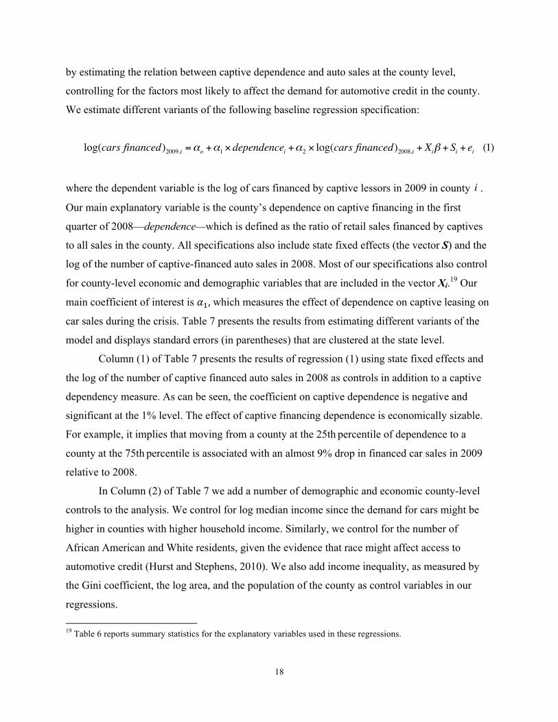
We estimate different variants of the following baseline regression specification:

log(cars financed)2009,i =αo +α1 × dependencei +α2 × log(cars financed)2008,i + Xiβ + Si + ei (1)

where the dependent variable is the log of cars financed by captive lessors in 2009 in county .

Our main explanatory variable is the county’s dependence on captive financing in the first

quarter of 2008—dependence—which is defined as the ratio of retail sales financed by captives

to all sales in the county. All specifications also include state fixed effects (the vector S) and the

log of the number of captive-financed auto sales in 2008. Most of our specifications also control

for county-level economic and demographic variables that are included in the vector Xi.19 Our

main coefficient of interest is 𝛼!, which measures the effect of dependence on captive leasing on

car sales during the crisis. Table 7 presents the results from estimating different variants of the

model and displays standard errors (in parentheses) that are clustered at the state level.

Column (1) of Table 7 presents the results of regression (1) using state fixed effects and

the log of the number of captive financed auto sales in 2008 as controls in addition to a captive

dependency measure. As can be seen, the coefficient on captive dependence is negative and

significant at the 1% level. The effect of captive financing dependence is economically sizable.

For example, it implies that moving from a county at the 25th percentile of dependence to a

county at the 75th percentile is associated with an almost 9% drop in financed car sales in 2009

relative to 2008.

In Column (2) of Table 7 we add a number of demographic and economic county-level

controls to the analysis. We control for log median income since the demand for cars might be

higher in counties with higher household income. Similarly, we control for the number of

African American and White residents, given the evidence that race might affect access to

automotive credit (Hurst and Stephens, 2010). We also add income inequality, as measured by

the Gini coefficient, the log area, and the population of the county as control variables in our

regressions.                                                                                                                          19 Table 6 reports summary statistics for the explanatory variables used in these regressions.

i

19  

We attempt to address concerns about omitted variable bias by controlling for the fraction

of county-level employment in automobile manufacturing. As illustrated in Fig. 4, counties in

Michigan—the headquarters of the “big three”— as well as counties in states where auto

manufacturers have a longstanding presence such as Alabama, Indiana, Kentucky, and

Tennessee, have the largest share of captive-financed transactions in the United States. The

empirical concern is that in areas with strong employment links to the automotive sector, the

demand for cars might endogenously vary with the health of that sector. We address this concern

directly by controlling for the relative size of employment in automobile manufacturing within

the county.20

The inclusion of these county-level variables, which are not available for every county in

our data, results in a slightly smaller sample size: 2,849 in Column (2) compared to 3,082 in

Column (1). As Column (2) shows, the point estimate on captive dependence declines by about

20% from -0.635 to -0.469 but remains significant at the 1% level, still suggesting that the loss of

captive-financing capacity might have had a large, independent impact on car sales in this period.

Among the sociodemographic variables, we find that both median income and the number of

African American residents in the county are correlated with the number of car sales financed by

captive lessors. Available on request are results that combine the 2005–2009 ACS with county-

level data from the 2000 Census in order to compute the change in median income, the poverty

rate, population, and African American population inside the county over the two periods. The

point estimate on the captive dependence variable is unchanged.

Although the specification in Column (2) controls for a battery of economic and

demographic characteristics, there is a burgeoning literature on the effect of home prices and

household leverage during the boom on local demand and employment (see Mian and Sufi,

forthcoming, 2011; and the broader discussion in Mian and Sufi, 2014b). As a result, to the

extent that captive dependence is correlated with this demand channel, estimates of the

dependence coefficient might be biased.

We address this concern in Column (3) of Table 7 by adding the 2009 county-level

unemployment rate as well the median debt to income ratio for households in a county in 2006 to

the control variables used in Column (2). These data are available for a smaller subsample of

                                                                                                                         20 Appendix A provides a detailed description of variables construction and their sources.

20  

counties, reducing the sample size from 2,849 in Column (2) to 979 counties in Column (3). Yet

the negative impact of dependence remains robust, with statistical significance at the 1% level

and a point estimate that is very close to the one obtained in Column (1). Interestingly, in these

specifications that include captive dependence as the main explanatory variables and in contrast

to some of the earlier studies we do not find an independent statistically significant effect of

unemployment and household debt on car sales that are financed by captive lessors.

Recent research has identified housing price changes as a chief catalyst behind the

collapse in household demand. In order to address further concerns about latent demand, Column

(4) directly controls for the average change in home prices in a county from 2008 to 2009. As

Column (4) of Table 7 demonstrates, the inclusion of housing price change—which, consistent

with the literature, is positive and statistically significant—does not affect our main finding. The

coefficient on captive dependence remains statistically significant and similar in magnitudes to

the estimates obtained in Columns (1) and (3). The housing price change point estimate suggests

that moving from a county at the 25th to the 75th percentile in this variable is associated with a

2% percent increase in car sales, suggesting that household net worth is an important factor in

car sales. But in this subsample, a similar change in captive dependence is associated with an 8%

drop in sales. In unreported results we also control for the median credit score in the county and

obtain similar results for the captive dependence estimates in Table 7.

We now consider additional robustness tests using the regression reported in Column (2)

as our baseline specification.

6.2. Placebo and robustness

One concern about our analysis is the endogeneity of captive-leasing dependence, where our

measure of captive dependence captures an omitted demand factor. For example, it is possible

that counties in which captive lessors are more prevalent are also counties that experienced a

general decline in consumption of durable goods during the crisis. In order to address this

concern, we supplement our analysis with a placebo exercise and report the results in Table 8.

We use the same regression specification as in Table 7, Column (2). However, we

redefine the dependent variable to be the log number of cars that were bought for cash within a

county in 2009. If captive dependence merely captures unobserved county-level demand, then, as

in the estimates reported in Table 7, 𝛼!, the coefficient of captive dependence, should be

21  

negative and significant. In contrast, the results of the placebo test, reported in Table 8, Column

(1), show that 𝛼! is very close to zero and is statistically not significant. That is, we find no

effect of a county’s dependence on captive leasing on overall cash sales of cars, and hence we

can reject the notion that our measure of captives captures a general demand side factor. The fact

that captives are associated with lower sales of financed cars but do not affect cash sales of

automobiles reinforces our argument that our results are driven by a credit supply shock.

Furthermore, we obtain data from Nielsen on the dollar value of consumer expenditure at

the county level. The Nielsen consumer expenditure data include purchases of apparel,

education, electronic devices, food, furniture, major appliances, medical expenses, and personal

care. If captive dependence merely proxies for latent demand, then counties with greater captive

dependence should have also experienced a greater decline in other purchases during this period.

In contrast, as Column 3 of Table 8 shows, the point estimate on captive dependence is both

economically and statistically insignificant, suggesting that it unlikely that our measure of

captive dependence captures latent demand.

We have already addressed the concern that captive dependence is higher in counties

with a large automotive sector by directly controlling for the fraction of county-level

employment in automobile manufacturing in Table 7. We refine this control in Columns (2) and

(3) of Table 8 by splitting the sample between counties with and without auto industry

employment and estimating specification (1) separately for each of the samples. These

regressions focus on counties that—based on employment data—have no ties to the auto

industry; hence, their dependence on captive leasing is unlikely to be specifically correlated with

the state of the industry. Column (2) of Table 8 reports results that are based on the sample of

2,003 counties in which there is zero employment in the auto industry, while Column (3)

coefficients are estimated with a sample of the 846 counties with strictly positive auto industry

employment. As Column (2) shows, the point estimate of captive dependence in the zero auto

employment is negative and statistically significant at the 1% level. As expected, the coefficient

of captive dependence is higher in counties with links to the auto industry (-0.556 compared to -

0.476). Nevertheless, the coefficient in Column (2) of Table 8 is almost identical to the estimate

obtained in our baseline specification in Column (2) of Table 7 (-0.476 compared to -0.469). We

conclude that our results are unlikely to be driven by local employment effects of the automotive

industry.

22  

6.3. Captive dependence and aggregate auto sales

The evidence in Table 7 shows that captive financed auto sales fell after the collapse of the

ABCP market in those areas more heavily dependent on captive financing. However, other

lenders such as banks could have stepped in as alternative sources of finance—substituting for

the loss of captive-financing capacity. And this potential substitution effect—away from captive

lenders—could partially or even fully mute the adverse effects of captive distress on car sales.

We examine the substitution hypothesis and report results in Table 9 using the same benchmark

specification presented in Column (2) of Table 7.

Column (1) of Table 9 uses the log number of non-captive financed transactions within a

county in 2009 as the dependent variable: these transactions include all banks and financing

companies that are not captive arms of the automakers. As Table 9 shows, the point estimate on

captive dependence is now positive and statistically significant. In particular, moving from a

county at the 25th percentile to the 75th percentile of captive dependence is associated with a

1.8% increase in non-captive financed sales. This change in sign—compared to the estimates for

captive leasing in Table 7—suggests that as captives reduced their credit supply, other lenders

were providing an alternative source of credit. These results remain robust if we also include the

change in house prices and household leverage.

Moreover, this evidence for partial substitution from captive lessors to other financial

intermediaries lends credence to the credit supply shock hypothesis and our identification

strategy. If our captive dependence measure primarily proxies for weak demand within a county

during the crisis, then even the number of non-captive transactions should have fallen as well,

and hence the coefficient in Column (1) would have been expected to be negative. Instead, the

contrast in the sign of the captive dependence coefficients between Tables 7 and 9 suggest that

our results are unlikely to be driven by latent demand, but rather reflect the effects of diminished

captive credit supply on auto sales in this period.

The evidence presented in the first column of Table 9 suggests that some financial

intermediaries stepped in to fill the void left by captive lessors. We now turn to analyze the

aggregate consequences of the contraction in captive credit supply. To do so, we redefine the

dependent variable as the log of the number of all car sales in a county in 2009, regardless of

whether they were financed or the source of financing. As Column 2 of Table 9 demonstrates,

23  

the dependence coefficient is negative and statistically significant at the 1% level. Moving from

a county at the 25th percentile to the 75th percentile of captive dependence is associated with

2.5% drop in overall car sales in 2009. Thus, substitution away from captive lessors into other

lenders may have only partially muted the impact of captive distress on lending and auto sales.

And as before, these findings are unchanged if we control for house price changes and household

leverage and their interaction.

We argue that the main reason that banks could not fully substitute for the decline in

credit supply by captive lessors is driven by informational frictions. As discussed in Section 2,

the vertical integration of captive lessors into auto manufacturers enables them to overcome

informational frictions surrounding collateral values. This informational advantage helps captive

lessors in providing both floorplan credit to auto dealerships as well as credit in the form of

leases and loans to consumers.21

6.4. The home price and household leverage channels in auto sales

The last column of Table 7 shows that changes in house prices are positively correlated with auto

sales, and in Table 10, we investigate in greater detail how local home prices and household

leverage might have shaped auto sales during this period (Mian and Sufi (2010, 2011) and Mian,

Rao and Sufi (2013)).

The first column of Table 10 repeats the analysis presented in Column 4 of Table 7. The

effect of captive dependence in this subsample is about four times higher than the home price

effect, while household leverage has no effect on auto sales. We conjecture that household

leverage does not seem to be an important determinant of auto sales in this subsample since the

automobiles are financed through auto loans and leases and hence rely less on home equity. We

next turn to estimate the importance of household leverage and house prices for cars bought with

cash – where home equity and household leverage may play a bigger role. As Column 2 of Table

10 demonstrates, and consistent with the placebo results in Column 1 of Table 8, captive leasing

is unrelated to car cash sales. In contrast, household leverage and house price changes are both

statistically and economically significant in explaining cash car sales, confirming their

                                                                                                                         21 See Pierce (2012) for evidence suggesting that captive lessors have informational advantage in predicting lease

residual values—although these advantages may be mitigated by conflicting interests within the organization.

24  

importance for cars that are not financed by captive lessors. The housing price change point

estimate suggests that moving from a county at the 25th to the 75th percentile in this variable is

associated with a 4% percent increase in car sales. Similarly, moving from the 25th to the 75th

percentile in household leverage increases is associated with a 2 percent increase in car sales.

Finally, the last column of Table 10 reports the coefficients for aggregate car sales. While

both captive dependence and housing prices are statistically significant at the one percent level,

household leverage is only marginally significant. These estimates likely reflect the composition

of the new car auto market in the U.S. in which more than 80% of the cars are financed by

captive leases and auto loans from leasing companies and other financial institutions, and only

20% are bought for in all cash transactions.

6.5. Changes in aggregate financing capacity and local auto sales

The panel structure of our data can help in providing more direct evidence linking changes in

captive-financing capacity to the local supply of credit and auto sales. The approach builds on

the idea that because money market funds—mutual funds that invest in short-term securities—

are the principal source of funding for many securitization conduits, we would expect that when

net flows into MMFs are plentiful, these funds are likely to increase their demand for captive

ABCP.22 This in turn could lead captives to increase the supply of captive credit to dealers and

households. Conversely, a sharp contraction in MMF net inflows would be expected to increase

the cost of ABCP financing for captives, leading to a contraction in captive credit supply and

slower captive-financed sales growth.

Using data from Flow of Funds, Fig. 5 plots the net inflows into MMFs during the crisis.

Net inflows into funds that primarily serve retail investors were far less volatile during this

period than flows into those funds that cater to institutional investors—the latter were the major

buyers of ABCP during this period.

We would thus expect that the effects of MMF flows on the financing capacity of

captives are likely to be more pronounced in those counties more dependent on captive

financing. And we exploit the variation in both the cross-section of captive dependence and the

                                                                                                                         22 MMF can be grouped by type of investments. Treasury MMF sole invest in Treasury securities. Non-Treasury

MMF also buy commercial paper from non-financial firms and ABCP conduits.

25  

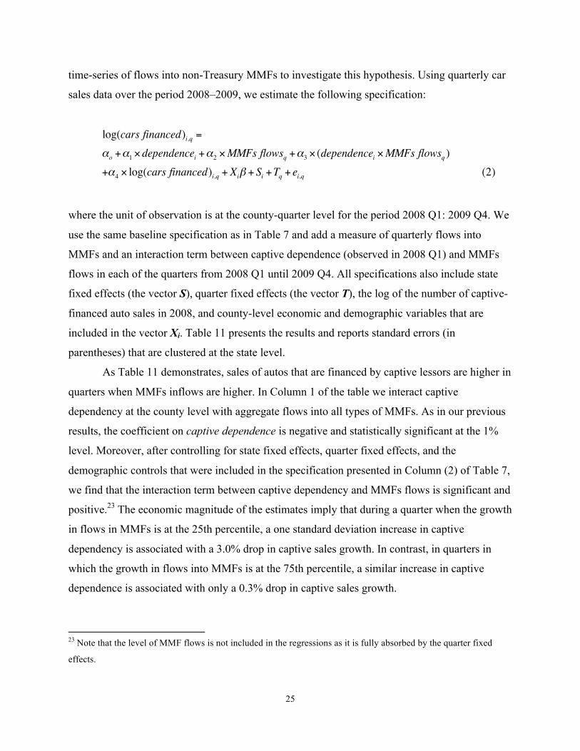
time-series of flows into non-Treasury MMFs to investigate this hypothesis. Using quarterly car

sales data over the period 2008–2009, we estimate the following specification:

log(cars financed)i,q =αo +α1 × dependencei +α2 ×MMFs flowsq +α3 × (dependencei ×MMFs flowsq )+α4 × log(cars financed)i,q + Xiβ + Si +Tq + ei,q (2)

where the unit of observation is at the county-quarter level for the period 2008 Q1: 2009 Q4. We

use the same baseline specification as in Table 7 and add a measure of quarterly flows into

MMFs and an interaction term between captive dependence (observed in 2008 Q1) and MMFs

flows in each of the quarters from 2008 Q1 until 2009 Q4. All specifications also include state

fixed effects (the vector S), quarter fixed effects (the vector T), the log of the number of captive-

financed auto sales in 2008, and county-level economic and demographic variables that are

included in the vector Xi. Table 11 presents the results and reports standard errors (in

parentheses) that are clustered at the state level.

As Table 11 demonstrates, sales of autos that are financed by captive lessors are higher in

quarters when MMFs inflows are higher. In Column 1 of the table we interact captive

dependency at the county level with aggregate flows into all types of MMFs. As in our previous

results, the coefficient on captive dependence is negative and statistically significant at the 1%

level. Moreover, after controlling for state fixed effects, quarter fixed effects, and the

demographic controls that were included in the specification presented in Column (2) of Table 7,

we find that the interaction term between captive dependency and MMFs flows is significant and

positive.23 The economic magnitude of the estimates imply that during a quarter when the growth

in flows in MMFs is at the 25th percentile, a one standard deviation increase in captive

dependency is associated with a 3.0% drop in captive sales growth. In contrast, in quarters in

which the growth in flows into MMFs is at the 75th percentile, a similar increase in captive

dependence is associated with only a 0.3% drop in captive sales growth.

                                                                                                                         23 Note that the level of MMF flows is not included in the regressions as it is fully absorbed by the quarter fixed

effects.

26  

One concern about these results is that we are capturing some general trend in economic

conditions rather than actual flows into MMFs. In order to address this concern, we conduct

robustness tests in which we control for the S&P 500 index level, real GDP, State-level income

as well as the interaction of these variables with captive dependence. Our results (which are

omitted for brevity and are available upon request) are unaffected by the inclusion of these time-

series economic indicators and their interactions with county-level captive dependence.

Next, we further split MMFs flows between institutional MMFs and retail MMFs. Not all

MMFs invest in ABCP: while MMFs that primarily cater to retail investors tend to be more

conservative and were less likely to invest in ABCP, institutional MMFs invested in riskier

assets such as ABCP (Kacperczyk and Schnabl, 2013). As Columns (2) and (3) of Table 11

show, our results are driven by institutional MMF flows (point estimate of 0.023 significant at

the 5% level in Column 2 compared to an insignificant 0.005% in Column 3). Taken together,

the results in Table 11 suggest that shocks to the financing capacity provided by MMFs, mainly

those funds focused on institutional investors, had a significant impact on the collapse in car

sales during the financial crisis and the great recession.

6.6. Make heterogeneity and county fixed effects

We now turn to analyze the heterogeneity of the effect of captive leasing on auto sales. More

specifically, we study the effect of captive leasing on sales within auto manufacturers.24 In each

of the columns of Table 12 we restrict our analysis to only one automaker in each regression and

estimate specifications similar to Regression (1) with the same set of control variables as in

Column (2) of Table 7. In each of the columns in the table captive dependence is defined as a

county’s dependence on the captive-financing arms of each of the automakers based on sales

financed in 2008 Q1. The table reports results for the three largest automakers in the United

States: GM, Columns (1)–(3); Ford, Columns (4)–(6); and Toyota, Columns (7)–(9).

The dependent variable in Column (1) of Table 12 is the change in GMAC-financed sales

within a county from 2008 to 2009. As the table shows, the point estimate on GMAC

dependence is negative and significant, suggesting that the collapse in GMAC-financed sales                                                                                                                          24 There is evidence that concerns about the long-term solvency of the automobile manufacturer could independently

shape the demand for its cars (see Hortacsu, Matvos, Syverson, and Venkataraman, 2013).

27  

was larger in those areas more dependent on GMAC for credit: a one standard deviation increase

in dependence is associated with a 0.14 standard deviation drop in the change in GMAC sales.

While Non-GMAC financed GM sales rose sharply in those areas where GMAC was more

dominant (Column 2), the net aggregate impact on GM sales is negative despite the substitution

away from GMAC-financed cars (Column 3).

In results available on request, we also use a change in GMAC’s credit policy to connect

further the availability of financing from short-term funding markets and captive credit supply.

This test is motivated by the fact that in early October 2008, GMAC found it increasingly

difficult to roll over its debt in the ABCP market and decided to strategically reallocate its

remaining financing capacity away from borrowers with a credit score of less than 700

(Congressional Oversight Panel, 2013). The TARP injection in late December 2008 relieved

some of these funding pressures, and GMAC lowered its credit score requirement to 620.

Consistent with this credit supply narrative, we find evidence that those counties that are more

dependent on GMAC for their GM car purchases and have a larger fraction of borrowers with

credit scores below 700 suffered a steeper collapse in GM car sales in the fourth quarter of 2008

relative to those counties that relied on other lenders to supply car credit and had better credit

scores.

The remaining columns of Table 12 repeat the basic specifications for the other two

major makes in the United States: Ford and Toyota. The pattern is similar across the three largest

automakers. It suggests that despite the variation in experiences across these firms, dependence

on captive financing played a significant role in explaining some of the collapse in car sales.

Last, the richness of our data and in particular, the availability of make level data allow

us to once more gauge the extent of biased estimates due to latent county-level unobservables

that might both explain the demand for cars within a county and its dependence on captive

financing. Specifically, we use a different aggregation of the data where the unit of observation

is at the make-county level for the four largest automakers: Toyota, GM, Ford, and Honda.25 The

                                                                                                                         25 Together, these four makes accounted for about 55% of the US market in 2007, have a market presence across

most geographic regions, and offer models in most segments. We exclude smaller makes, such as Nissan, the next

largest car company in terms of market share in the Polk data, as these firms tend to operate in only a small number

of counties and compete in only one or two segments. For example, while the Ford Taurus and various Buick

 

28  

make-county data aggregation enables us to control for county fixed effects as well as make

fixed effects in our regression analysis.

This specification thus absorbs any latent time invariant county- and make-level effects

and offers a powerful robustness check. For example, a county’s exposure to the “cash for

clunkers” program, as determined by the preexisting fraction of “clunkers” in the county’s

automobile stock, could be correlated with both sales in 2009 and captive dependency (Mian and

Sufi, 2012). Similarly, a county’s industrial structure, such as the degree of employment in

nontraded goods, or its indirect connections to the automobile sector not measured by BLS

employment shares, could also drive demand and correlate with the captive dependency, leading

to biased estimates.

More specifically, we estimate the following regression model:

log(cars financed)2009,i,m =αo +α1 × dependencei,m +α2 × log(cars financed)2008,i,m+α3 × (market share)2008,i,m +Ci +Mm + ei,m (3)

where the unit of observation is at the county-make level. All specifications also include the log

number of car sales financed by captives in 2008 Q1. And since we now disaggregate the data by

make, we can include the market share of the make within a county in 2008 Q1, as well as

county fixed effects (the vector C) and make fixed effects (the vector M). Table 13 presents the

results and reports standard errors (in parentheses) that are clustered at the state level.

As Column (1) of Table 13 shows, the impact of captive dependence on captive-financed

sales remains negative and statistically significant at the 1% level after controlling for both

county and make fixed effects. While there is also evidence of substitution (Column 2), the

coefficient is imprecisely estimated and is not statistically significant. Last, the net aggregate

effect of captive dependency remains negative and significant after controlling for county fixed-

effects (Column 3). Our main result thus holds within each county across different makes and

controlling for make-specific effects.

The results presented in the first three columns of Table 13 are important in alleviating

                                                                                                                                                                                                                                                                                                                                                                                                       models compete in the “large sedan” segment, Nissan offers no models in that segment. Likewise, Subaru sells

almost no new cars in the South and competes in only a handful of segments.

29  

concerns about unobserved county and automaker invariant effects. However, the automobile

market is highly segmented, and this segmentation suggests that even after controlling for county

and make fixed effects, shocks to the demand for cars within a county could vary substantially

across models, even for those sold by the same firm. For example, some manufacturers, such as

GM, offer a large number of makes and models aimed at buyers with different income levels:

Chevrolet, a major sub-make within GM, generally sells nonluxury models that are marketed

toward lower- and middle-income buyers, while Buick and Cadillac, again both GM sub-makes,

sell more luxurious models aimed at higher-income buyers.26 As a result, the collapse in house

prices and the rise in household leverage among lower-income borrowers could precipitate a

drop in the demand for Chevrolet models within a county, whereas demand for Buick and

Cadillac cars within the same county could be less affected. In contrast, housing price dynamics

may have had a smaller impact on the net worth of these higher-income buyers. Thus, one can

argue that our measure of captive leasing captures those households who traditionally bought

nonluxury models and that were more affected by the drop in housing prices such as subprime

borrowers.

Using the detailed model and make data from Polk, along with information on model

types from Wards Automotive, one of the standard purveyors of intelligence on the automotive

industry, we augment our analysis to utilize within-make within-county within-segment

heterogeneity. Wards Automotive identifies the market segment in which each car model

competes, and we use this information to construct a county-make-segment panel: the number of

cars that each make sold within each county in each market segment. The market segmentation

in the industry can be highly detailed, and Ward’s lists 30 segments. This level of granularity

can, however, lead to a large number of missing observations in our data set, as specialized

models, such as the Chevrolet Corvette, tend to have a small number of sales in a limited

geographic area. We thus collapse the 30 segments in Wards into eight broad market segments

that correspond to the Insurance Institute for Highway Safety’s classification: small cars; mid-

sized cars; large cars; luxury cars; small utility vehicles; mid-sized utility vehicles; large utility

                                                                                                                         26 Even within some sub-makes such as Chevrolet, some models, such as the Corvette, are aimed at richer buyers.

Bricker, Ramcharan, and Krimmel (2014) and the references contained discuss cars, status, and the marketing of

cars in the United States.

30  

vehicles; and luxury utility vehicles.27

With information on county, make, and segment, we can include make fixed effects, Mm

, county fixed effects, Ci , and county-segment fixed effects,µis . As before, make fixed effects

allow us to absorb any shocks to make-level sales that affects all counties and segments, such as

the potential insolvency of a make, while county fixed effects continue to absorb county-specific

time-invariant factors that affect sales of all cars equally within the county. The addition of

county-segment fixed effects now absorbs invariant factors that affect sales of a particular

segment that vary across segments, even within the same county. Our modified regression

specification is:

log(cars financed)2009,i,m,s =αo +α1 × dependencei,m,s +α2 × log(cars financed)2008,i,m,s+α3 × (market share)2008,i,m,s +Ci +Mm +µi,s + ei,m (4)

As Column (4) of Table 13 demonstrates, our basic results remain the same when controlling for

county-segment fixed effects. A one standard deviation increase in captive dependence measured

is associated with about a 1.2% drop in sales in 2009. In results available upon request, we

replicate this exercise at the more aggregate MSA level, including all mainstream makes and

models—our basic results are unchanged. In summary, the combined evidence in Table 13

renders it unlikely that our results are driven by omitted county or automaker factors. More

important, the last column of the table shows that our results hold when we compare cars that are

sold within county and auto segment, and thus it is unlikely that our captive dependence measure

is capturing latent demand for cars.

7. Banks and the collapse of auto sales

After presenting evidence on the collapse of the ABCP market and its effect on captive lessors

and car sales, we now turn to analyze the effect of ABCP on bank auto loans. Some banks were

heavily exposed to the ABCP market, incurring losses either directly through their sponsorship

of automobile-related conduits or indirectly via an increase in funding costs (Acharya and Mora,

2013). Bank-level data thus allow us to test further how disruptions in these markets might have

affected the availability of automotive credit, which led to a decline in car sales.                                                                                                                          27 Appendix B provides more details on how the Wards data are merged to Polk.

31  

To this end, we hand matched the credit supplier names from Polk with the income and

balance sheet data available in banks’ Call Reports. In cases where a bank is part of a bank

holding company, we aggregate the Call Report data up to the bank holding company level and

collectively refer to both stand-alone banks and bank holding companies as banks. The names of

banks in the Polk data set do not always correspond to the legal names of the banks as recorded

in the Call Report—especially for the smaller banks. Our Call Reports–Polk-matched sample has

about 1,500 banks that are, on average, larger than the entire population of banks.28

Similar to Acharya and Mora (2013), we use two proxies for a bank’s reliance on short-

term wholesale funding. First, we construct a bank’s unused commitments ratio: the ratio of

unused loan commitments to the sum of loans and unused commitments. Unused loan

commitments are the parts of credit lines that have not been drawn down and include, for

example, support to ABCP program conduits that the banks were not required to consolidate on

their balance sheets before the crisis. Banks with a higher precrisis unused commitments ratio are

thus more heavily active in short-term markets and as a result are more exposed to stresses in

these markets. The second proxy is the net wholesale funding ratio—liabilities excluding core

deposits—divided by total assets. Banks that are less reliant on core deposits—a stable source of

funding—are likely to have been more exposed to the disruptions in short-term funding markets

during the crisis.

Table 14 reports results from bank-level regressions. For the 1,534 banks in our cross-

section, we regress the log number of cars financed in 2009 on our two measures of a bank’s

exposure to short-term funding markets, observed in 2006. We also control for the log number of

cars financed in 2008 by the bank, along with a number of bank-level characteristics from 2006,

such as: bank assets (log), the ratio of Tier 1 capital to assets, the loans to assets ratio, and the

share of real estate loans on the bank’s balance sheet. As the table demonstrates, the estimated

coefficient on the wholesale funding ratio is negative and significant at the 10% level. A one

standard deviation increase in dependence on wholesale funding in 2006 is associated with a 6%

drop in total cars financed in 2009. The point estimate on the unused commitments ratio is also

negative but is not statistically significant. Last, and not surprisingly, there is also evidence that

                                                                                                                         28 For example, the average bank in our sample had around $45 billion in assets in 2007, while the average for the

full sample of banks in the Call Reports is $32 billion.

32  

those banks more exposed to the real estate sector during the boom contracted automotive credit

more sharply.

Our central thesis is that contraction in aggregate credit supply affects economic activity

adversely and that this was the case during the financial crisis of 2008–2009. The adverse effects

were not confined only to the time of the crisis, however. Some of the large-scale changes in

financial regulation that followed the crisis made it more expensive for banks, especially the

larger banks, to engage in many forms of securitization and to access wholesale funding markets.

In particular, in 2009, the Financial Accounting Standards Board modified accounting

standards so that transfers of assets by banks to SPVs would no longer be recognized as a sale.

Instead, these new rules required banks, beginning in 2010, to consolidate the assets and

liabilities of any supported SPVs into the balance sheet of the bank holding company for

regulatory and financial reporting purposes, thereby broadening the range of assets subject to

capital requirements and decreasing the attractiveness of off-balance sheet securitization (FASB

Statement Nos. 166 and 167). 29 Concurrently, banking regulators also announced a sizable

expansion in capital and liquidity requirements, especially for the larger banks.30 Non-bank

lenders such as Ford Motor Credit are largely exempt from many of these capital and liquidity

requirements, while many smaller banks face relatively lower requirements.31 All this suggests

that banks more connected to these markets would be expected to contract automotive credit

more sharply, especially after these regulatory changes.

If these results reflect the effects of a loss of financing capacity stemming from the

disruptions in the ABCP and other short-term funding markets, then the aforementioned 2009–

2010 regulatory changes would be expected to engender an even sharper contraction in credit                                                                                                                          29 Summaries of these statements can be found here:

http://www.fasb.org/cs/ContentServer?pagename=FASB%2FPronouncement_C%2FSummaryPage&cid=11761562

41369. 30 The regulatory agencies’ amendment of their bank capital adequacy frameworks in response to the FASB rule on

the consolidation of ABCP programs can be found here: http://www.fdic.gov/news/board/DEC152009no2.pdf.

Other regulatory changes pertaining to securitization also focus on risk retention, the role of credit agencies, and the

Volcker Rule. A general survey of the various US and international changes to bank capital and liquidity

requirements and other regulations after the crisis is here: http://www.stlouisfed.org/federal-banking-regulations/. 31 To be sure, the Dodd-Frank Act of 2010 allows the Federal Reserve to regulate non-bank financial institutions if

they are deemed systemically important.

33  

supply for those banks more dependent on these markets in the boom.

Column (2) of Table 14 uses the total number of cars financed 2010–2013 as the

dependent variable, controlling for the standard suite of bank-level controls, as well as the log

number of cars financed in 2009. As Column (2) shows, both the wholesale funding ratio and the

unused commitments variables are significant at the 1% level. The point estimates are also much

larger. A one standard deviation increase in the former is associated with an 11.5% drop in car

sales. In the case of the latter, a similar increase is associated with a 9% drop in sales over the

2010–2013 period. Thus, the disruptions in short-term markets and some of the postcrisis

regulatory changes intended to make banks less reliant on short-term credit markets might have

curtailed the supply of credit, resulting in a prolonged contraction.

8. Captive leasing in the post-crisis years

These aforementioned post crisis changes in financial regulation aimed at banks relative to

non-banks offer yet another way to gauge the importance of captive financing capacity on car

sales.32 Funding in ABS securitization markets in the post crisis period have become increasingly

stable and cheap funding, yet banks face higher costs to securitization relative to the pre-crisis

regulatory environment. Table 15 thus investigates the extent to which captives relative to other

intermediaries might have used ABS securitization markets to gain market share from the

traditional banking system.

Using a quarterly panel for the period 2010-2013, column 1 regresses the growth in

aggregate sales in a county on captive dependence. Captive dependence is also interacted with

the spread between the A-rated tranche of auto ABS over the corresponding two-year interest

rate swap. The interaction term is negative and significant. This suggests that captive credit

supply tends to decline in periods when the cost of funding in these markets rise,

disproportionately affecting sales in those counties more dependent on captive financing.

Column 2 shows the supply of bank credit is however relatively insensitive to the cost of funding

in these markets: the interaction term is not significant. Column 3 replicates these results using

                                                                                                                         32  In  comparison  to  the  larger  number  of  new  regulations  aimed  at  banks  that  have  emerged  after  the  passage  of  the  Dodd-­‐Frank  Act,  non-­‐bank  automotive  finance  companies  have  only  recently  attracted  the  attention  of  federal  regulators:  http://www.consumerfinance.gov/newsroom/cfpb-­‐proposes-­‐new-­‐federal-­‐oversight-­‐of-­‐nonbank-­‐auto-­‐finance-­‐companies/  

34  

the BBB spread. The coefficients are more precisely estimated but similar in magnitude to the

previous results, suggesting that the relative calm in securitization markets post-crisis, along with

the various changes in regulation aimed at banks, may have increased the financing capacity of

captives relative to other lenders.

9. Conclusion

There is now considerable evidence that balance-sheet shocks to traditional financial institutions

may have limited the availability of credit to the real economy. Our paper contributes to this

literature in two ways. First, we show the real consequences of credit supply by linking shocks to

short-term funding markets to credit supply by captive leasing companies and auto sales. Second,

we provide evidence that illiquidity in the short-term funding markets played an important role in

limiting the supply of non-bank consumer credit during the financial crisis. The collapse of the

ABCP market decimated the financing capacity of many captive financing companies as well as

some large banks. Our paper documents the importance of leasing companies in the provision of

credit in the auto markets and the consequential real effects that credit supply had on auto

purchases during the financial crisis and the great recession.

35  

References

Acharya, V., Mora, N., 2013. A crisis of banks as liquidity providers. Journal of Finance,

forthcoming.

Acharya, V., Schnabl, P., Suarez, G., 2011. Securitization without risk transfer. Journal of

Financial Economics 107, 515–536.

Adams, W., Einav, L., Levin, J., 2009. Liquidity constraints and imperfect information in

subprime lending. American Economic Review 99, 49–84.

Allen, F., Babus, A., Carletti, E., 2009. Financial crisis: theory and evidence. Annual Review of

Financial Economics 1, 97–116.

Allen, F., Gale, D., 2000. Financial contagion. Journal of Political Economy 108, 1–33.

Barron, J., Chong, B.-U., Staten, M., 2008. Emergence of captive finance companies and risk

segmentation in loan markets: theory and evidence. Journal of Money, Credit and Banking 40,

173–192.

Bricker, J., Ramcharan, R., Krimmel, J., 2014. Signaling status: the impact of relative income on

household consumption and financial decisions. Available at SSRN:

http://dx.doi.org/10.2139/ssrn.2435503.

Brunnermeier, M., 2009. Deciphering the liquidity and credit crunch 2007–08. Journal of

Economic Perspectives 23, 77–100.

Calder, L., 1999. Financing the American Dream: A Cultural History of Consumer Credit.

Princeton University Press, Princeton.

Campbell, S., Covitz, D., Nelson, W., Pence, K., 2011. Securitization markets and central

banking: an evaluation of the term asset-backed securities loan facility. Journal of Monetary

Economics 58, 518–531.

Charles, K., Hurst, E., Stephens, M., Jr., 2010. Rates for vehicle loans: race and loan source.

American Economic Review 98, 315–320.

36  

Chodorow-Reich, G., 2014. The employment effects of credit market disruptions: firm-level

evidence from the 2008–09 financial crisis. Quarterly Journal of Economics 129, 1–59.

Cornett, M., McNutt, J., Strahan, P., Tehranian, H., 2011. Liquidity risk management and credit

supply in the financial crisis. Journal of Financial Economics 101, 297–312.

Covitz, D., Liang, N., Suarez, G., 2013. The evolution of a financial crisis: collapse of asset-

backed commercial paper market. Journal of Finance 68, 815–848.

Diamond, D., Rajan, R., 2005. Liquidity shortages and banking crisis. Journal of Finance 60,

615–647.

Diamond, D., Rajan, R., 2011. Fear of fire sales, illiquidity seeking, and credit freezes. Quarterly

Journal of Economics 126, 557–591.

Einav, L., Jenkins, M., Levin, J., 2012. Contract pricing in consumer credit markets.

Econometrica 80, 1387–1432.

Einav, L., Jenkins, M., Levin, J., 2013. The impact of credit scoring on consumer credit. RAND

Journal of Economics 44, 249–274.

Gorton, G., 2010. Slapped by the Invisible Hand: The Panic of 2007. Oxford University Press,

Oxford.

Gorton, G., Metrick, A., 2012. Securitized banking and the run on repo. Journal of Financial

Economics 104, 425–451.

Haugh, D., Mourougane, A., Chatal, O., 2010. The automobile industry in and beyond the

crisis.” OECD Economics Department Working Paper No. 745.

Hyman, L., 2011. Debtor Nation: The History of America in Red Ink. Princeton University

Press, Princeton.

Ivanshina, V., Scharfstein, D., 2010. Bank lending during the financial crisis of 2008. Journal of

Financial Economics 97, 319–338.

37  

Kacperczyk, M., Schnabl, P., 2013. How safe are money market funds? Quarterly Journal of

Economics, forthcoming.

Khwaja, A., Mian, A., 2008. Tracing the impact of bank liquidity shocks: evidence from an

emerging market. American Economic Review 98, 1413–1442.

Ludvigson, S., 1998. The channel of monetary transmission to demand: evidence from the

market for automobile credit. Journal of Monetary Economics 30, 365–383.

Mian, A., Rao, K., Sufi, A., 2013. Household balance sheets, consumption and the economic

slump. Quarterly Journal of Economics 128, 1687–1726.

Mian, A., Sufi, A., 2010. Household leverage and the recession of 2007–09. IMF Economic

Review 58, 74–114.

Mian, A., Sufi, A., 2011. House prices, home equity-based borrowing, and the U.S. household

leverage crisis. American Economic Review 101, 2132–2156.

Mian, A., Sufi, A., 2012. The effects of the fiscal stimulus: evidence from the 2009 Cash for

Clunkers program. Quarterly Journal of Economics 1107–1142.

Mian, A., Sufi, A., 2014a. What explains the 2007–2009 drop in employment? The aggregate

demand channel. Unpublished working paper. Princeton University.

Mian, A., Sufi, A., 2014b. House of Debt: How They (and You) Caused the Great Recession,

and How We Can Prevent It from Happening Again. University of Chicago Press, Chicago.

Mufin, J., Pratt, R., 2014. Captive finance and the coase conjecture. Unpublished working paper,

Yale School of Management.

Phelps, C., 1952. The Role of the Sales Finance Companies in the American Economy.

Schneidereith and Sons, Baltimore.

Pierce, L., 2012. Organizational structure and the limits of knowledge sharing: incentive conflict

and agency in car leasing. Management Science 58, 1106–1121.

Pozsar, Z., Adrian, T., Ashcraft, A., Boesky, H., 2010. Shadow banking. FRBNY Staff Report

No. 458.

38  

Rajan, Raghuram, and Rodney Ramcharan, The Anatomy of a Credit Crisis: The Boom and Bust

in Farm Land Prices in the United States in the 1920s, forthcoming, American Economic Review.

Ramcharan, R., Verani, S., van den Heuvel, S.,. From Wall Street to Main Street: the impact of

the financial crisis on consumer credit, forthcoming, Journal of Finance

Ramcharan, R. and Crowe, Christopher. 2013. “The Impact of House Prices on Consumer

Credit: Evidence From an Internet Bank.” Journal of Money, Credit and Banking 45(6): 1085–

1115.

Shleifer, A., Vishny, R., 2010. Unstable banking. Journal of Financial Economics 97, 306–318.

Sloan, A., 1964. My Years with General Motors. Doubleday, New York.

39  

Appendix A: Variable Description and Construction

For reference, the following is a list of variables used in the paper, their sources, and a brief description of

how each variable is constructed.

i. African American Population: Number of African Americans in a county. (Source: American

Community Survey)

ii. Assets: Total bank assets. (Source: FR Y9-C, FFIEC 031)

iii. Captive Dependence: Share of county-level retail car sales financed by captive financing

companies. (Source: Polk)

iv. Captive Financed Sales: County-level retail car sales financed by captive financing companies.

(Source: Polk)

v. County Area: Size of a county in square miles. (Source: American Community Survey)

vi. Employment in Automobile Manufacturing: Divides the number of employees in the automobile

sector by total employment. (Source: Quarterly Census of Employment and Wages)

vii. Gini Coefficient: Measures income inequality in a county. (Source: American Community

Survey)

viii. House Price Change: Annual change in the local house price index. (Source: CoreLogic)

ix. Household Leverage: County-level household debt-to-income ratio. (Source: Federal Reserve of

New York)

x. Leverage Ratio: Divides Tier 1 eligible equity capital by total bank assets. (Source: FR Y9-C,

FFIEC 031)

xi. Loans/Assets: Total bank loans divided by total bank assets. (Source: FR Y9-C, FFIEC 031)

xii. Median Household Income (Source: American Community Survey)

xiii. Money Market Fund Flows: Quarterly net flows to (from) money market funds. (Source: Flow of

Funds, Federal Reserve Board)

xiv. Non-Captive Financed Sales: County-level retail car sales not financed by captive financing

companies. (Source: Polk)

xv. Percent African American: African American population divided by population. (Source:

American Community Survey)

xvi. Population: Number of people in a county. (Source: American Community Survey)

xvii. Population density: Population divided by area. (Source: American Community Survey)

xviii. Poverty Rate: Number of people living below the poverty line divided by population. (Source:

US Census)

40  

xix. Real Estate Loans/Assets: Total real estate loans divided by total bank assets. (Source: FR Y9-C,

FFIEC 031)

xx. Retail Car Sales: The sum of retail purchases and retail leases. (Source: Polk)

xxi. Unemployment Rate: county-level labor force divided by the number of unemployed. (Source:

BLS)

xxii. Unused Commitments Ratio: Total unused commitments divided by the sum of total unused

commitments and total loans. (Source: FR Y9-C, FFIEC 031)

xxiii. White Population: Number of Caucasians in a county. (Source: American Community Survey)

xxiv. Wholesale Deposits/Assets: Total uninsured deposits divided by total bank assets. (Source: FR

Y9-C, FFIEC 031)

41  

Appendix B: Auto Segment Construction

The eight auto segments used in make-county regression (Table 11) include the following models:

i. Small Cars (WARD categories: lower small and upper small)

BMW 128, BMW 135, Chevrolet Aveo, Chevrolet Cobalt, Dodge Caliber, Ford Focus, Honda Civic,

Honda Fit, Hyundai Accent, Hyundai Elantra, Kia Rio, Kia Forte, Kia Soul, Kia Spectra, Mazda 3, Mini

Cooper, Mitsubishi Lancer, Nissan Cube, Nissan Sentra, Nissan Versa, Pontiac G3, Pontiac Vibe, Saab 93,

Saturn Astra, Saturn Ion, Subaru Impreza, Suzuki Aerio, Suzuki Forenza, Suzuki Reno, Suzuki SX4,

Toyota Corolla, Toyota Yaris, Volkswagen GLI, Volkswagen Golf, Volkswagen Jetta, Volkswagen R32,

Volkswagen Rabbit, Volvo V50.

ii. Mid-sized Cars (WARD categories: lower middle and upper middle)

Buick Lacrosse, Chevrolet Impala, Chevrolet Malibu, Chrysler Sebring, Dodge Avenger, Ford Fusion,

Honda Accord, Honda FCX, Honda Insight, Hyundai Azera, Hyundai Sonata, Kia Optima, Mazda 6,

Mercury Mila, Mercury Montego, Mercury Sable, Mitsubishi Galant, Nissan Altima, Pontiac G6, Pontiac

G8, Pontiac Grand Prix, Saturn Aura, Subaru Legacy, Suzuki Kizashi, Toyota Camry, Volkswagen CC,

Volkswagen Passat, Volvo V70.

iii. Large Cars (WARD category: large)

Buick Lucerne, Chrysler 300, Dodge Charger, Dodge Magnum, Ford Crown Victoria, Ford Five Hundred,

Ford Taurus, Kia Amanti, Mercury Grand Marquis, Mercury Monterey.

iv. Luxury Cars (WARD categories: small luxury, middle luxury, and large luxury)

Acura RL, Acura TL, Acura TSX, Audi A3, Audi A4, Audi A6, Audi S4, Bentley Continental, BMW 328,

BWM 335, BW 525, BMW 528, BMW 530, BMW 535, BMW 550, BMW M3, BMW M5, Cadillac CTS,

Cadillac DTS, Cadillac STS, Chevrolet Monte Carlo, Hyundai Genesis, Infiniti G35, Infiniti G37, Infiniti

M35, Infiniti M45, Jaguar S-Type, Jaguar X-Type, Lexus ES, Lexus GS, Lexus HS250H, Lexus IS,

Lincoln MKS, Lincoln MKZ, Lincoln Town Car, Mercedes-Benz C-Class, Mercedes-Benz CLK-Class,

Mercedes-Benz E-Class, Nissan Maxima, Toyota Avalon, Volvo S40, Volvo S60, Volvo S80.

v. Small Utility Vehicles (WARD categories: small cross/utility and small sport/utility)

Chevrolet HHR, Chrysler PT Cruiser, Dodge Nitro, Honda Element, Hyundai Tucson, Jeep Compass, Jeep

Liberty, Jeep Patriot, Jeep Wrangler, Kia Sportage, Land Rover LR2, Mercury Mariner, Saab 95, Suzuki

Grand Vitara.

vi. Mid-Sized Utility Vehicles (WARD categories: middle cross/utility and middle sport/utility)

Chevrolet Equinox, Chevrolet Trailblazer, Dodge Journey, Ford Edge, Ford Escape, Ford Explorer, GMC

Envoy, GMC Terrain, Honda CR-V, Honda Crosstour, Honda Pilot, Hyundai Santa Fe, Hyundai Veracruz,

Isuzu Ascender, Jeep Commander, Jeep Grand Cherokee, Kia Borrego, Kia Rondo, Kia Sorento, Land

Rover LR3, Mazda 5, Mazda CX-7, Mazda Tribute, Mitsubishi Endeavor, Mitsubishi Outlander, Nissan

Murano, Nissan Pathfinder, Nissan Rogue, Nissan Xterra, Pontiac Torrent, Saturn Vue, Subaru B9 Tribeca,

42  

Subaru Forester, Subaru Outback, Suzuki XL7, Toyota 4 Runner, Toyota FJ Cruiser, Toyota Highlander,

Toyota RAV4, Toyota Venza, Volkswagen Tiguan.

vii. Large Utility Vehicles (WARD categories: large cross/utility and large sport/utility)

Buick Enclave, Chevrolet Suburban, Chevrolet Tahoe, Chevrolet Traverse, Chrysler Aspen, Dodge

Durango, Ford Expedition, Ford Flex, Ford Freestyle, Ford Taurus X, GMC Acadia, GMC Envoy XL,

GMC Yukon, Mazda CX-9, Mitsubishi Montero, Nissan Armada, Saturn Outlook, Toyota Sequoia.

viii. Luxury Utility Vehicles (WARD categories: small luxury cross/utility, middle luxury cross/utility,

large luxury cross/utility, luxury middle sport/utility, and luxury large sport/utility)

Acura MDX, Acura RDX, Acura ZDX, Audi Q5, Audi Q7, BMW X3, BMW X5, BMW X6, Buick

Rainier, Buick Rendezvous, Cadillac Escalade, Cadillac SRX, Chrysler Pacifica, Hummer 4-PSGR Wagon,

Hummer H2, Hummer H3, Infiniti EX, Infiniti FX35, Infiniti FX45, Infiniti FX50, Infiniti QX56, Land

Rover LR4, Land Rover Range Rover, Lexus GX, Lexus LX, Lexus RX, Lincoln MKT, Lincoln MKX,

Lincoln Navigator, Mercedes-Benz G-class, Mercedes-Benz GL-class, Mercedes-Benz GLK, Mercedes-

Benz M-class, Mercedes-Benz R-class, Mercury Mountaineer, Porsche Cayenne, Saab 9-7X, Subaru

Tribeca, Toyota Land Cruiser, Volkswagen Touareg, Volvo XC60, Volvo XC70, Volvo XC90.

43  

Figure 1. Outstanding Issuances of Asset-Backed Commercial Paper. Outstanding stock asset-

backed commercial paper issued by three captive finance companies, 2006 Q1–2009 Q4. Source: Moody’s Investor

Services.

05

1015

2025

2006q1 2007q1 2008q1 2009q1 2010q1date

Chrysler Financial Ford Motor CreditGeneral Motors Acceptance Corp

billio

ns

44  

Figure 2a. Total Car Sales, 2002–2013. Total annual car purchases in Polk.

45  

Figure 2b: Total Retail Car Sales, 2002–2013. Retail car sales are the sum of retail leases and retail

purchases in Polk.

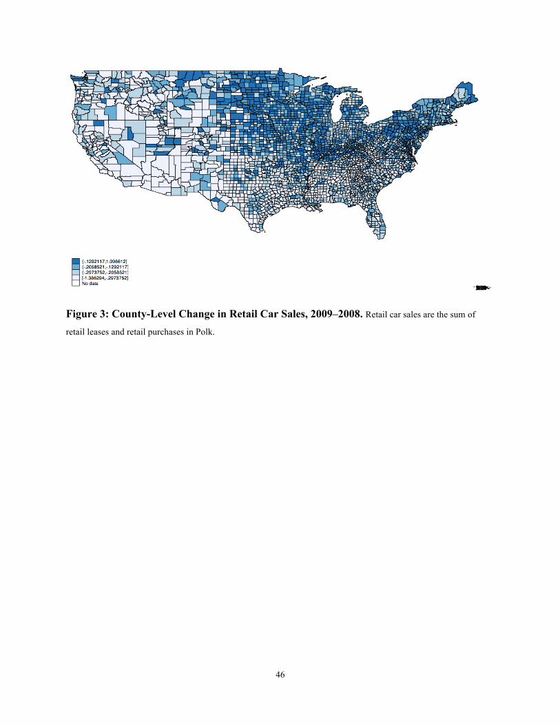
46  

Figure 3: County-Level Change in Retail Car Sales, 2009–2008. Retail car sales are the sum of

retail leases and retail purchases in Polk.

47  

Figure 4. County-Level Share of Retail Cars Financed by Captives in 2008Q1. Retail car sales

are the sum of retail leases and retail purchases in Polk.

48  

Figure 5. Quarterly Net Flows to Money Market Funds, 2008–2009. Flows are calculated using

data from Flow of Funds.

49  

Table 1. Market Share of the Financial Intermediaries in the Supply of Consumer Credit

This table lists the market share of various sources of consumer credit before, in, and after the financial crisis. Panel

A reports the market shares for total installment credit. Panel B reports the market share for the subset of auto loans.

Consumer credit data are taken from the Flow of Funds.

A. Total Consumer Installment Credit (%)

By holder By originator

2005 2009 2010 2005 2009 2010

Credit Unions 13.9 12.9 12.2 13.9 12.9 12.2

Commercial Banks 27.4 31.4 33.2 28.3 32.1 33.2

Finance Companies 47.8 45.2 38.1 41.8 37.9 35.5

B. Auto Loan Market Share (%)

2005 2009 2010

Credit Unions 20.8 23.6 24.1

Commercial Banks 24.1 32.6 37.0

Finance Companies 51.3 41.3 36.7

50  

Table 2. Automobile Captives and Commercial Paper, 2005 This table lists the percentage of commercial paper in all liabilities (bank loans, notes, bonds, and debentures, debt

due to parent firm, and other liabilities excluding equity and retained earnings) in 2005 for four major automobile

captives operating in the United States. The data are supervisory and non-public.

Captive 1 2 3 4

Share of Commercial Paper 66.67 45.91 10.23 75.12

Table 3. Summary Statistics of County-Level Retail Sales

This table presents the summary statistics for retail car sales across all counties for each year. Retail sales are the

sum of retail purchases and retail leases in Polk. The sample period is 2002 to 2013.

Year Mean

Standard

Deviation Min

25th

Percentile Median

75th

Percentile Max

2002 4,210 14,323 2 343 886 2,464 420,627

2003 4,251 13,945 1 340 868 2,485 420,561

2004 4,173 14,269 1 347 875 2,508 443,374

2005 4,096 14,343 2 331 845 2,405 456,466

2006 3,996 14,082 2 327 820 2,360 443,677

2007 3,866 13,331 1 321 808 2,332 409,445

2008 3,168 10,651 3 273 678 1,931 314,265

2009 2,563 8,334 2 219 528 1,553 235,562

2010 2,771 9,115 1 237 565 1,664 259,567

2011 3,113 10,045 3 280 667 1,926 287,269

2012 3,553 11,945 3 313 746 2,191 367,536

2013 3,881 13,342 3 329 795 2,343 417,487

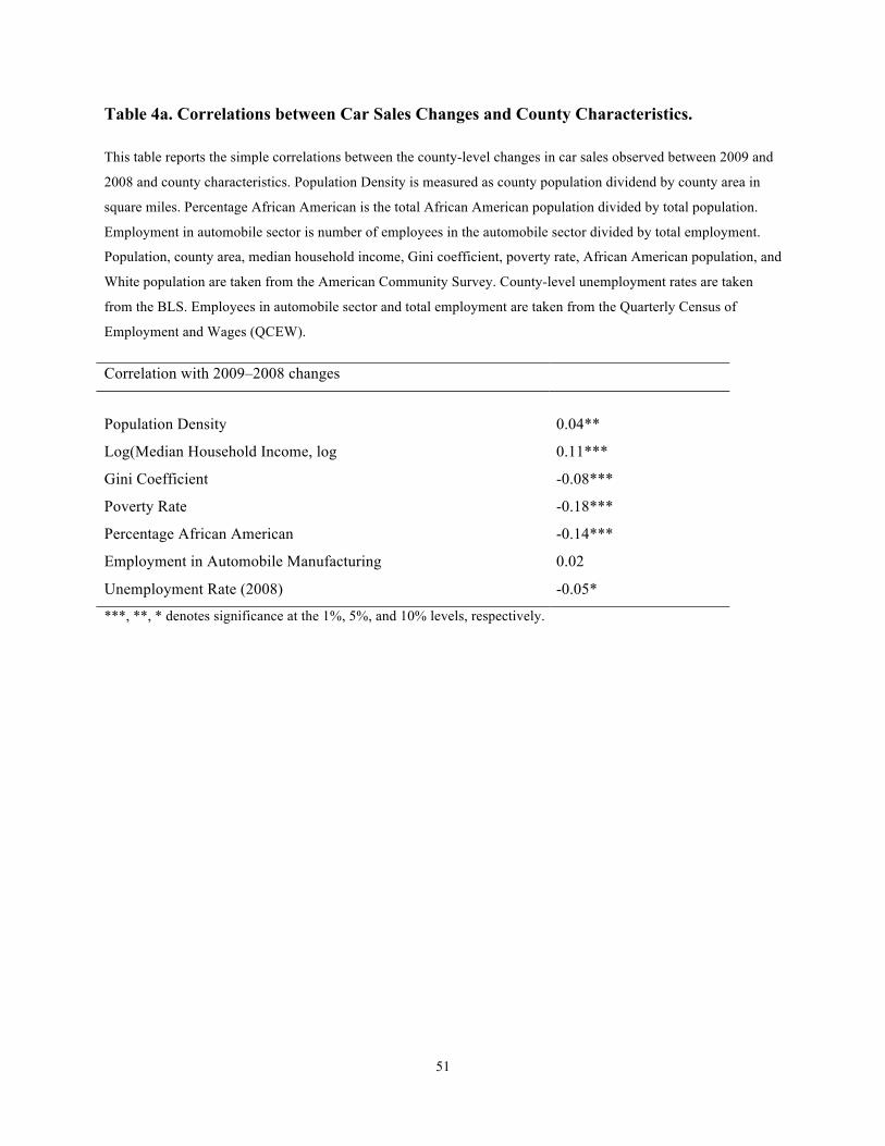
51  

Table 4a. Correlations between Car Sales Changes and County Characteristics.

This table reports the simple correlations between the county-level changes in car sales observed between 2009 and

2008 and county characteristics. Population Density is measured as county population dividend by county area in

square miles. Percentage African American is the total African American population divided by total population.

Employment in automobile sector is number of employees in the automobile sector divided by total employment.

Population, county area, median household income, Gini coefficient, poverty rate, African American population, and

White population are taken from the American Community Survey. County-level unemployment rates are taken

from the BLS. Employees in automobile sector and total employment are taken from the Quarterly Census of

Employment and Wages (QCEW).

Correlation with 2009–2008 changes

Population Density 0.04**

Log(Median Household Income, log 0.11***

Gini Coefficient -0.08***

Poverty Rate -0.18***

Percentage African American -0.14***

Employment in Automobile Manufacturing 0.02

Unemployment Rate (2008) -0.05*

***, **, * denotes significance at the 1%, 5%, and 10% levels, respectively.

52  

Table 4b. Car Sales Changes and County Characteristics. This table reports the regression results of regression county-level car sales changes observed between 2009 and 2008 on county characteristics. Population Density is measured as county population dividend by county area in square miles. Percentage African American is the African American population divided by population. Employment in automobile sector is number of employees in the automobile sector divided by total employment. Population, county area, median household income, Gini coefficient, poverty rate, African American population, and White population are taken from the American Community Survey. County-level unemployment rates come from the BLS. Employees in automobile sector and total employment are taken from the Quarterly Census of Employment and Wages (QCEW). Variables (1) (2) (3) (4) (5) (6) (7) (8)

Population Density 3.04e-06*

2.95e-06**

(1.60e-06)

(1.42e-06)

Median Income, log

0.062***

-0.0857***

(0.012)

(0.0252)

Poverty Rate

-0.004***

-0.00606***

(0.0005)

(0.00118)

Percentage African American

-0.141***

-0.102***

(0.0166)

(0.0259)

Gini Coefficient

-0.325***

0.133

(0.0898)

(0.125)

Employment in Automobile

Manufacturing

0.213*

0.107

(0.129)

(0.140)

Unemployment Rate (2008)

-0.004** 0.00263

(0.0017) (0.00186)

Observations 3,108 3,108 3,108 3,108 3,108 3,103 2,550 2,546

R-squared 0.001 0.011 0.032 0.020 0.007 0.000 0.003 0.043

***, **, * denotes significance at the 1%, 5%, and 10% levels, respectively.

53  

Table 5. GMAC Financing

This table presents the market shares of GMAC in retail and wholesale financing of GM car sales. Column (1)

reports the percent of dealer floor plan financing supplied by GMAC. Column (2) reports the percent of GM sales—

in units—financed by GMAC. The financing shares are taken from GMAC 10-Ks.

Year GMAC Floorplan Financing—

Percentage of GM Dealers

GMAC Consumer Automobile

Financing—Percentage of GM Sales

2005 82 36

2006 80 38

2007 82 35

2008 81 32

2009 78 20

Table 6. Summary Statistics

This table presents the summary statistics for county characteristics used in the empirical analysis. Captive

dependence is the market share of captive finance companies in a county as of 2008:Q1. Population, county area,

median household income, Gini coefficient, poverty rate, African American population, and White population are

taken from the American Community Survey. Employees in automobile sector and total employment are taken from

the Quarterly Census of Employment and Wages (QCEW).

Variable Mean

Standard

Deviation Min

25th

Percentile Median

75th

Percentile Max

Captive Dependence 0.39 0.1 0.08 0.32 0.38 0.45 1

County Area, log 6.42 1 0.69 6.04 6.4 6.82 11.89

Population, log 10.25 1.45 4.36 9.32 10.16 11.06 16.09

Median Income, log 10.64 0.29 9.33 10.49 10.64 10.79 11.65

African American Population, log 6.78 2.59 0 4.92 6.95 8.71 14.11

White Population, log 10.04 1.45 3.04 9.12 9.99 10.92 15.42

Gini Coefficient 0.43 0.04 0.21 0.41 0.43 0.46 0.65

Employment in Automobile Sector, share 0.004 0.01 0 0 0 0.0003 0.19

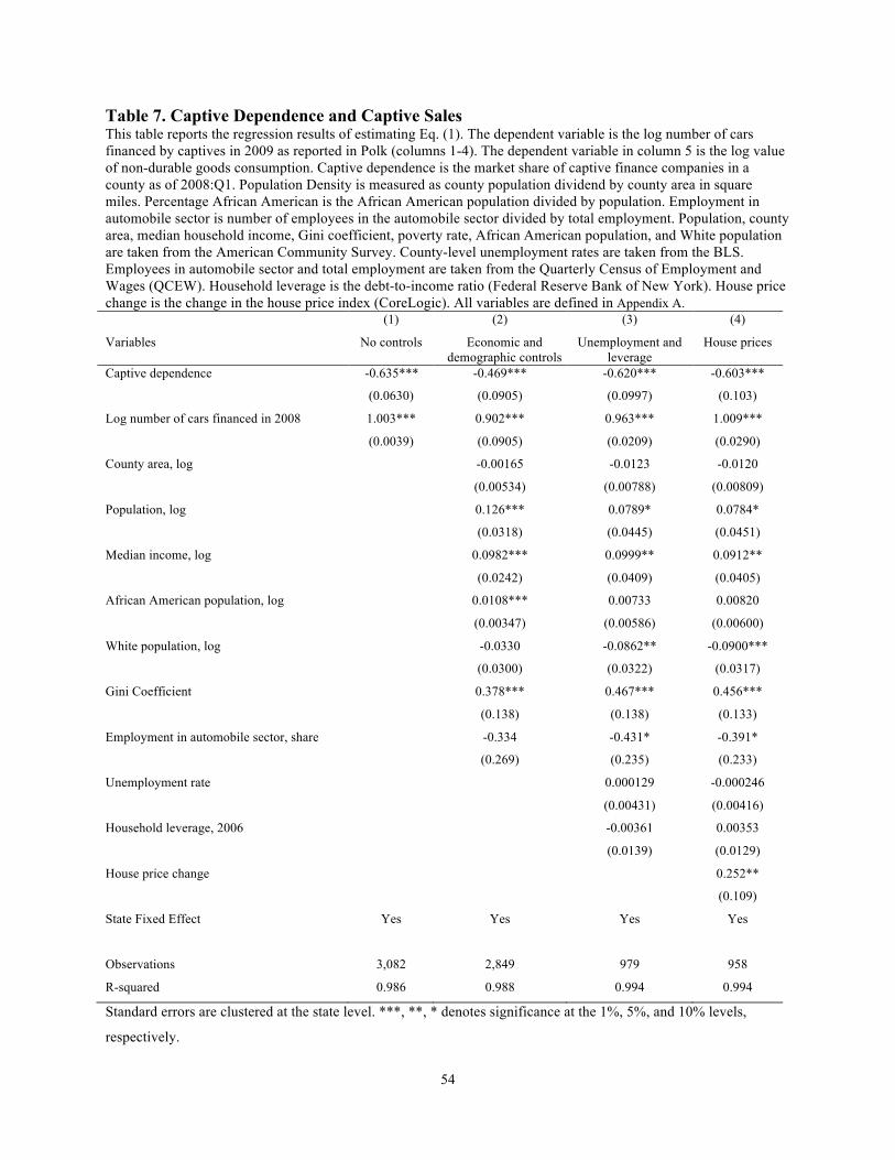
54  

Table 7. Captive Dependence and Captive Sales This table reports the regression results of estimating Eq. (1). The dependent variable is the log number of cars financed by captives in 2009 as reported in Polk (columns 1-4). The dependent variable in column 5 is the log value of non-durable goods consumption. Captive dependence is the market share of captive finance companies in a county as of 2008:Q1. Population Density is measured as county population dividend by county area in square miles. Percentage African American is the African American population divided by population. Employment in automobile sector is number of employees in the automobile sector divided by total employment. Population, county area, median household income, Gini coefficient, poverty rate, African American population, and White population are taken from the American Community Survey. County-level unemployment rates are taken from the BLS. Employees in automobile sector and total employment are taken from the Quarterly Census of Employment and Wages (QCEW). Household leverage is the debt-to-income ratio (Federal Reserve Bank of New York). House price change is the change in the house price index (CoreLogic). All variables are defined in Appendix A. (1) (2) (3) (4)

Variables   No controls   Economic and demographic controls  

Unemployment and leverage  

House prices  

Captive dependence -0.635*** -0.469*** -0.620*** -0.603***

(0.0630) (0.0905) (0.0997) (0.103)

Log number of cars financed in 2008 1.003*** 0.902*** 0.963*** 1.009***

(0.0039) (0.0905) (0.0209) (0.0290)

County area, log -0.00165 -0.0123 -0.0120

(0.00534) (0.00788) (0.00809)

Population, log 0.126*** 0.0789* 0.0784*

(0.0318) (0.0445) (0.0451)

Median income, log 0.0982*** 0.0999** 0.0912**

(0.0242) (0.0409) (0.0405)

African American population, log 0.0108*** 0.00733 0.00820

(0.00347) (0.00586) (0.00600)

White population, log -0.0330 -0.0862** -0.0900***

(0.0300) (0.0322) (0.0317)

Gini Coefficient 0.378*** 0.467*** 0.456***

(0.138) (0.138) (0.133)

Employment in automobile sector, share -0.334 -0.431* -0.391*

(0.269) (0.235) (0.233)

Unemployment rate 0.000129 -0.000246

(0.00431) (0.00416)

Household leverage, 2006 -0.00361 0.00353

(0.0139) (0.0129)

House price change 0.252**

(0.109)

State Fixed Effect Yes Yes Yes Yes

Observations 3,082 2,849 979 958

R-squared 0.986 0.988 0.994 0.994

Standard errors are clustered at the state level. ***, **, * denotes significance at the 1%, 5%, and 10% levels,

respectively.

55  

Table 8. Robustness: Cash Sales Placebo and Auto Industry Employment This table reports the regression results of estimating Eq. (1). The dependent variable in Column (1) is the log number of cars bought with cash in 2009 as reported in Polk. The dependent variable in Column (2) is the log of the dollar amount of aggregate consumer expenditure at the county level in 2009 calculated by Nielsen. The dependent variable in Columns (3) and (4) is the log number of cars financed by captives in 2009 as reported in Polk. Captive dependence is the market share of captive finance companies in a county as of 2008:Q1. Population density is measured as county population dividend by county area in square miles. Percentage African American is the African American population divided by population. Employment in automobile sector is number of employees in the automobile sector divided by total employment. Population, county area, median household income, Gini coefficient, poverty rate, African American population, and White population are taken from the American Community Survey. Employees in automobile sector and total employment are taken from the Quarterly Census of Employment and Wages (QCEW).

(1)

 (2) (3) (4)

Dependent Variable

Cash Sales

Nielsen Consumer

Expenditure

Captive Sales Counties without auto industry employment

Captive Sales Counties with auto industry

employment Captive dependence -0.00627 -0.00200 -0.476*** -0.556***

(0.0729) (0.0217) (0.0928) (0.132)

Log Number of Sales 2008 0.802*** 0.000769 0.887*** 0.967***

(0.0285) (0.00281) (0.0293) (0.0308)

County area, log -0.00373 0.0160 -0.000987 -0.00348

(0.0105) (0.0158) (0.00597) (0.00853)

Population, log 0.121** -0.0392*** 0.130*** 0.0861*

(0.0521) (0.0119) (0.0401) (0.0497)

Median income, log 0.153*** 0.00396* 0.0726** 0.139***

(0.0432) (0.00230) (0.0284) (0.0352)

African American population, log -0.00392 -0.0163 0.0105** 0.00941

(0.00426) (0.0139) (0.00432) (0.00690)

White population, log 0.0813** -0.0532 -0.0257 -0.0608

(0.0391) (0.0544) (0.0331) (0.0447)

Gini Coefficient 0.282 0.106 0.324* 0.584***

(0.205) (0.125) (0.173) (0.162)

Employment in automobile, share -0.146 -0.00200

(0.162) (0.0217) State Fixed Effect Yes Yes Yes Yes

Observations 2,848 2,370 2,003 846

R-squared 0.986 0.989 0.975 0.994 Standard errors are clustered at the state level. ***, **, * denotes significance at the 1%, 5%, and 10% levels,

respectively.

56  

Table 9. Captive Dependence and Aggregate Effects.

This table reports regression results of estimating Eq. (1). The dependent variable in Column (1) is the log number

of cars financed by non-captives in 2009. The dependent variable in Column (2) is the log number of cars sold inside

the county in 2009. Captive dependence is the market share of captive finance companies in a county as of 2008:Q1.

The demographic controls are as the same as in Column (2) of Table 7. All variables are defined in Appendix A.

(1) (2)

Dependent variable Substitution Aggregate

Captive Dependence 0.149** -0.193***

(0.0631) (0.0533)

Log Number of Cars Financed in 2008 0.859*** 0.892***

(0.0281) (0.0229)

Demographic Controls Yes Yes

State Fixed Effects Yes Yes

Observations 2,848 2,849

R-squared 0.992 0.994

Standard errors are clustered at the state level. ***, **, * denotes significance at the 1%, 5%, and 10% levels,

respectively.

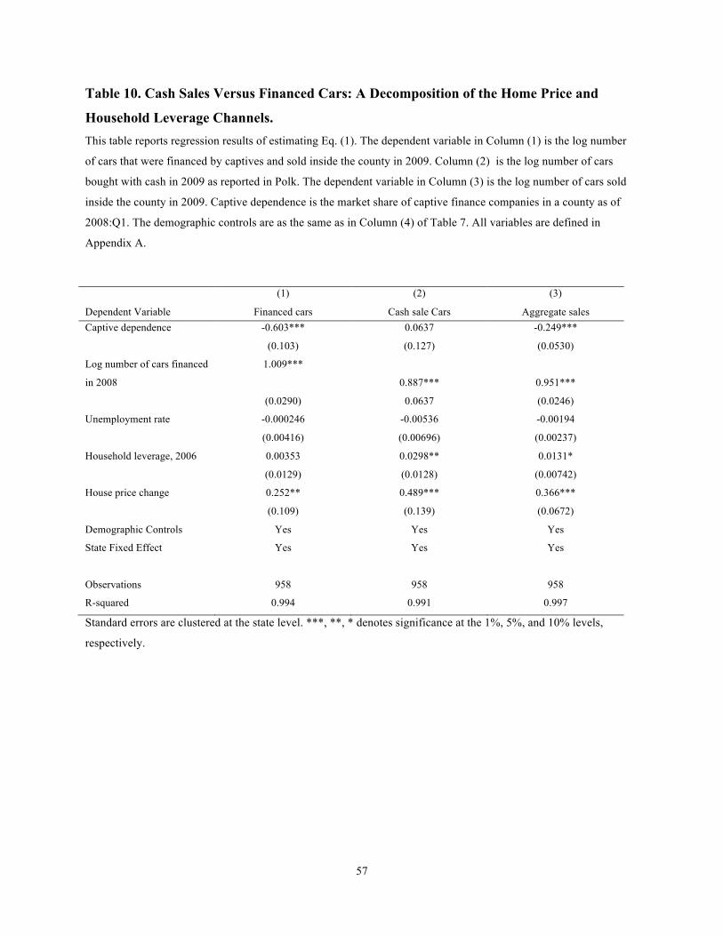
57  

Table 10. Cash Sales Versus Financed Cars: A Decomposition of the Home Price and

Household Leverage Channels. This table reports regression results of estimating Eq. (1). The dependent variable in Column (1) is the log number

of cars that were financed by captives and sold inside the county in 2009. Column (2) is the log number of cars

bought with cash in 2009 as reported in Polk. The dependent variable in Column (3) is the log number of cars sold

inside the county in 2009. Captive dependence is the market share of captive finance companies in a county as of

2008:Q1. The demographic controls are as the same as in Column (4) of Table 7. All variables are defined in

Appendix A.

(1) (2) (3)

Dependent Variable Financed cars Cash sale Cars Aggregate sales Captive dependence -0.603*** 0.0637 -0.249***

(0.103) (0.127) (0.0530)

Log number of cars financed

in 2008

1.009***

0.887*** 0.951***

(0.0290) 0.0637 (0.0246)

Unemployment rate -0.000246 -0.00536 -0.00194

(0.00416) (0.00696) (0.00237)

Household leverage, 2006 0.00353 0.0298** 0.0131*

(0.0129) (0.0128) (0.00742)

House price change 0.252** 0.489*** 0.366***

(0.109) (0.139) (0.0672)

Demographic Controls Yes Yes Yes

State Fixed Effect Yes Yes Yes

Observations 958 958 958

R-squared 0.994 0.991 0.997

Standard errors are clustered at the state level. ***, **, * denotes significance at the 1%, 5%, and 10% levels,

respectively.

58  

Table 11. Money Market Flows, Captive Dependence, and Car Sales

This table reports the results of estimating Eq. (2). The dependent variable is the quarterly growth in the number of

captive-financed transactions in county over the period 2008 Q2: 2009 Q4. Captive dependence is defined as the

fraction of retail car purchases financed by captive in 2008 Q1. Money market fund (MMF) flows are net inflows to

the respective fund category. Quarterly money market fund flow data are taken from the Flow of Funds. The

demographic controls are as the same as in Column (2) of Table 7.

(1) (2) (3)

Variables All MMFs Non-Treasuries

Institutional MMF Flows

Non-Treasuries

Retail MMF Flows

Captive Dependence -0.296*** -0.238*** -0.247***

(0.0482) (0.0232) (0.0335)

Captive Dependence * All MMF

Flows

0.0366*

(0.0211)

Captive Dependence * Institutional

MMF Flows

0.0227**

(0.00927)

Captive Dependence * Retail MMF

Flows

0.00480

(0.00452)

MMF flows Yes Yes Yes

Demographic Controls Yes Yes Yes

Year Fixed Effect Yes Yes Yes

Quarter Fixed Effect Yes Yes Yes

State Fixed Effect Yes Yes Yes

Observations 19,883 19,883 19,883

R-squared 0.451 0.432 0.444

Standard errors are clustered at the state level. ***, **, * denotes significance at the 1%, 5%, and 10% levels,

respectively.

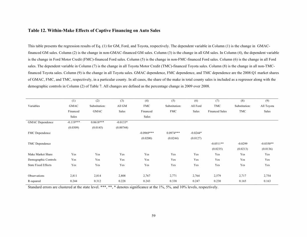
59  

Table 12. Within-Make Effects of Captive Financing on Auto Sales

This table presents the regression results of Eq. (1) for GM, Ford, and Toyota, respectively. The dependent variable in Column (1) is the change in GMAC-

financed GM sales. Column (2) is the change in non-GMAC-financed GM sales. Column (3) is the change in all GM sales. In Column (4), the dependent variable

is the change in Ford Motor Credit (FMC)-financed Ford sales. Column (5) is the change in non-FMC-financed Ford sales. Column (6) is the change in all Ford

sales. The dependent variable in Column (7) is the change in all Toyota Motor Credit (TMC)-financed Toyota sales. Column (8) is the change in all non-TMC-

financed Toyota sales. Column (9) is the change in all Toyota sales. GMAC dependence, FMC dependence, and TMC dependence are the 2008:Q1 market shares

of GMAC, FMC, and TMC, respectively, in a particular county. In all cases, the share of the make in total county sales is included as a regressor along with the

demographic controls in Column (2) of Table 7. All changes are defined as the percentage change in 2009 over 2008.

(1) (2) (3) (4) (5) (6) (7) (8) (9)

Variables GMAC

Financed

Sales

Substitution:

GMAC

All GM

Sales

FMC

Financed

Sales

Substitution:

FMC

All Ford

Sales

TMC

Financed Sales

Substitution:

TMC

All Toyota

Sales

GMAC Dependence -0.119*** 0.0618*** -0.0133*

(0.0309) (0.0145) (0.00744)

FMC Dependence -0.0969*** 0.0974*** -0.0244*

(0.0200) (0.0244) (0.0127)

TMC Dependence -0.0511** -0.0299 -0.0350**

(0.0235) (0.0213) (0.0136)

Make Market Share Yes Yes Yes Yes Yes Yes Yes Yes Yes

Demographic Controls Yes Yes Yes Yes Yes Yes Yes Yes Yes

State Fixed Effects Yes Yes Yes Yes Yes Yes Yes Yes Yes

Observations 2,811 2,814 2,808 2,767 2,771 2,764 2,579 2,717 2,754

R-squared 0.244 0.312 0.228 0.243 0.338 0.247 0.230 0.165 0.163

Standard errors are clustered at the state level. ***, **, * denotes significance at the 1%, 5%, and 10% levels, respectively.

60  

Table 13. Make-County Panel Regressions

This table reports the results of estimating Eq. (3). The makes are Ford, GM, Honda, and Toyota. The dependent

variable in Column (1) is the log number of cars financed by the automaker’s captive arm in 2009 within a county,

and Column (1) controls for the log number of cars financed by the automaker’s captive arm in 2008 within the

county. The dependent variable in Column (2) is the log number of cars not financed by the automakers’ captive

arms, and Column (2) controls for the log number of cars not financed by the automaker’s captive arm in 2008.

Column (3) is the log number of all sales inside the county in 2009, and Column (3) controls for the log number of

all sales in 2008. The dependent variable in Column (4) is the log number of all sales by a make in each of eight

segment (small cars; mid-sized cars; large cars; luxury cars; small utility vehicles; mid-sized utility vehicles; large

utility vehicles; and luxury utility vehicles; for details on the segments, see Appendix B) within a county in 2009;

the log number of sales in 2008 are included as a control variable. Market share is the fraction of cars sold by the

make in 2008:Q1 in the county. Column (4) measures market share as the fraction of cars sold by the make within

the segment in the county.

(1) (2) (3) (4)

Variables captive

transactions

substitution:

non-captive

transactions

all transactions all transactions

segments

Captive Dependence -0.306*** 0.0357 -0.0189* -0.0165**

(0.0323) (0.0325) (0.0101) (0.007)

Log Number of Cars Financed in 2008 Yes Yes Yes Yes

Market Share Yes Yes Yes Yes

Make Fixed Effect Yes Yes Yes Yes

County Fixed Effect Yes Yes Yes No

County-Segment Fixed Effect No No No Yes

Observations 11,526 11,546 11,624 33,844

R-squared 0.363 0.486 0.408 0.94

Standard errors are clustered at the state level. ***, **, * denotes significance at the 1%, 5%, and 10% levels,

respectively.

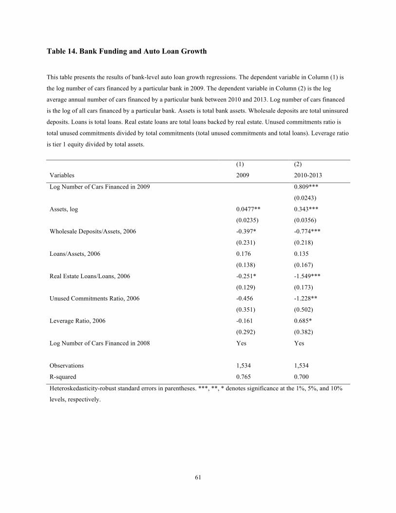
61  

Table 14. Bank Funding and Auto Loan Growth

This table presents the results of bank-level auto loan growth regressions. The dependent variable in Column (1) is

the log number of cars financed by a particular bank in 2009. The dependent variable in Column (2) is the log

average annual number of cars financed by a particular bank between 2010 and 2013. Log number of cars financed

is the log of all cars financed by a particular bank. Assets is total bank assets. Wholesale deposits are total uninsured

deposits. Loans is total loans. Real estate loans are total loans backed by real estate. Unused commitments ratio is

total unused commitments divided by total commitments (total unused commitments and total loans). Leverage ratio

is tier 1 equity divided by total assets.

(1) (2)

Variables 2009 2010-2013

Log Number of Cars Financed in 2009 0.809***

(0.0243)

Assets, log 0.0477** 0.343***

(0.0235) (0.0356)

Wholesale Deposits/Assets, 2006 -0.397* -0.774***

(0.231) (0.218)

Loans/Assets, 2006 0.176 0.135

(0.138) (0.167)

Real Estate Loans/Loans, 2006 -0.251* -1.549***

(0.129) (0.173)

Unused Commitments Ratio, 2006 -0.456 -1.228**

(0.351) (0.502)

Leverage Ratio, 2006 -0.161 0.685*

(0.292) (0.382)

Log Number of Cars Financed in 2008 Yes Yes

Observations 1,534 1,534

R-squared 0.765 0.700

Heteroskedasticity-robust standard errors in parentheses. ***, **, * denotes significance at the 1%, 5%, and 10%

levels, respectively.

62  

Table 15. The Recovery and Securitization, Quarterly growth in sales, 2010-2013 This table reports the results of estimating Eq. (2). The dependent variable is the quarterly growth in the number of

captive-financed transactions in county over the period 2010 Q1: 2013 Q4. Captive dependence is defined as the

fraction of retail car purchases financed by captive in 2008 Q1. Big bank dependence is the fraction of retail

purchases financed by the 20 largest banks—in terms of asset size—in 2008 Q1. Small bank dependence is the

fraction of retail purchases financed by all other banks in 2008 Q1. The A (BBB) spread is the spread between the

A(BBB)-rated tranche of auto ABS over the corresponding two year interest rate swap. The demographic controls

are as the same as in Column (2) of Table 7.

(1) (2) (3)

Variables captives captives and banks captives and banks: BBB spread

captive dependence 0.0604** 0.0607* 0.0878***

(0.0280) (0.0319) (0.0266)

captive dependence*A spread -0.000475* -0.000457

(0.000254) (0.000285)

big bank dependence -0.0113 -0.0183

(0.0445) (0.0380)

big bank dependence*A spread 0.000208

(0.000385)

small bank dependence 0.0186 0.0279

(0.0511) (0.0590)

small bank dependence*A spread -0.000125

(0.000458)

captive dependence*BBB spread -0.000398***

(0.000131)

big bank dependence*BBB spread 0.000154

(0.000191)

small bank dependence*BBB spread -0.000118

(0.000292)

Observations 45,672 45,672 45,672

R-squared 0.132 0.132 0.139