Liquidity Management and Monetary Policy∗

Javier Bianchi

University of Winsconsin and NBER

Saki Bigio

Columbia University

May 2013Preliminary and Incomplete

Abstract

We develop a novel theoretical framework to study monetary policy in conjunction

with an explicit role for banks. Banks are subject to a maturity mismatch problem

that leads to a precautionary motive for holding Central Bank reserves. Monetary

policy can have real and permanent effects by altering the trade-offs bank face between

lending, holding reserves, holding deposits and paying dividends. We use this frame-

work to analyze the macroeconomic effects of different monetary policy instruments

and regulatory constraints. We also study how these policy tools interact with exoge-

nous shocks to the volatility of withdrawals, equity losses and the demand for loans.

We then use a calibrated version of our model to investigate quantitatively how the

effectiveness of monetary policy may have changed in the aftermath of the 2008-2009

crisis, in response to these shocks and the regulatory constraints imposed by Basel-II.

∗We would like to John Cochrane, Nobu Kiyotaki, Arvind Krishnamurthy, Mike Woodford, Tomek Pisko-rski, Chris Sims and Harald Uhlig for discussing the ideas in this projects with us. As well we wish to thankseminar participants Columbia Macroeconomics Lunch, the Capital Theory Seminar at U Chicago and theMinneapolis Fed. Click here for Updates. Emails: jibianchi@wisc.edu and sbigio@columbia.edu

1

1 Introduction

The last five years have witnessed new challenges in the conduct of monetary policy. Dur-

ing the Great Recession, Central Banks were faced frozen inter-bank lending markets and

dropped their interest rate targets all the way to its zero lower-bound. At the peak of the

recession and even during its aftermath, Central Banks resorted to unconventional mone-

tary tools. By this, they purchased private paper and expanded their balance sheets in an

attempt to preserve financial stability and boost economic activity. These policies followed

events that dramatically affected the banking system. The financial crisis was a time where

the banking system saw unprecedented equity losses and banks responded by cutting back

on lending. In the aftermath, banks seem to have accumulated central bank reserves without

substantially resuming their lending in response to various monetary stimuli.1

These outcomes cast doubts about the effectiveness of monetary policy in stimulating

lending when the banking system is facing a substantial disruption. Despite the evident

connection between money and banking, there lacks a modern macroeconomic model that

enables the study of monetary policy in conjunction with an explicit role for banks.

In this paper, we take a step towards filling this gap. We propose a new theoretical frame-

work that focuses on some of the institutional details of banking to explain how monetary

policy is implemented. We build a theory that enables us to answer a number of theoretical

questions. How is the transmission monetary policy affected by the decisions of commercial

banks? How is this interaction affected by bank solvency and liquidity ratios? What is the

connection between monetary policy and financial regulation?2 What shocks can affect the

power of monetary policy?

We then use our theory to answer quantitative questions about the strength of monetary

policy in the last five years. In particular, we calibrate our model and use it to uncover the

type of shocks can explain the excess holdings of reserves by banks without a corresponding

increase in lending.

In our model the effectiveness monetary policy critically depends on the actions under-

taken by rational banks. Although the model is real, monetary policy carries real effects

through the lending channel. The model relies on a mechanism by which bank lending re-

acts to monetary policy because policy instruments alter the trade-offs between making a

profit on a loan against exposing a bank to more liquidity risk.

In essence, the heart of our model is a liquidity management problem. Banks choose the

optimal mix between lending, deposit issuance and holding bank reserves to hedge liquidity

1A summary of these events is presented later in the paper.2We refer to regulation such as the one put in place through the Dodd-Frank act or the Basel-III committee

on bank supervision.

2

risk. Liquidity risks are associated with financial losses that follow when deposits are with-

drawn and a bank does not have liquid reserves to comply with the command to transfer

deposits to another bank. The mechanics are the following. When a bank grants a loan, it

creates a liability in the form of a demand deposit. Granting a loan is profitable because a

higher interest is charged on the loan. However, there is a trade-off. More lending relative

to an amount reserves induces a potential maturity mismatch between bank assets, which

are long term, and deposits, which are callable at any time. We assume that loans cannot

be sold easily due to various frictions. Hence, banks hold central bank reserves (cash-like

securities) to meet an unexpected deposit withdrawal. However, it may well be that the

payment of bank liabilities exceeds their reserve levels. In such instances, banks must incur

in financial losses. These losses occur because they must obtain expensive borrowing from

the FED or other banks. Hence, holding more reserves, insures the bank against that risk.

We introduce this problem into a dynamic general equilibrium model with rational profit-

maximizing heterogeneous banks. The bank liquidity management problem is captured by a

portfolio with non-linear returns. The effects of monetary policy can be understood through

that liquidity-management portfolio problem. Thus, monetary policy operates by altering

the incentives that banks face when granting loans. Short-run monetary policy effects result

from the ability to alter the return to this portfolio problem. Long-run monetary-policy

effects are present because bank equity returns are affected. Consequently, the size of the

financial sector is also altered. An important feature of this channel is that monetary policy

can have real effects even if prices are fully flexible.

The implementation of monetary policy in our model is carried out through the use of

different policy instruments. We study the effects of discount rates, open market operations

(conventional and unconventional), reserve requirements and interests on reserves. All these

instruments have a common effect. They can tilt the balance towards a more lax lending

policy. The macroeconomic effects result from more lending and lower interest rates which

help stimulate economic activity. However, and this is the point we wish to convey in this

paper, is that as much as monetary policy can affect bank lending practices, in turn, its

power can be affected by other various circumstances that affect banking decisions.

The model delivers a rich description for banking and monetary indicators. For an

individual bank, it explains the behavior of their reserve holdings, lending policies, leverage

and dividend policies. For the banking industry as a whole, it provides descriptions of lending

volumes, interbank lending, excess reserve holdings. It also describes interbank borrowing

and lending rates. It also provides a description of banking financial indicators such as return

on loans, return on equity, banking dividend ratios as well as the book and market value

of banks. It has predictions about the size of the financial sector relative to the rest of the

3

economy. Finally, at the macroeconomic level, it provides a prediction about the evolution

of monetary aggregates, M0, M1 and the money multiplier.

We use these descriptions to explain the dynamic effects of aggregate outcomes to changes

in different monetary policy instruments and financial regulation. We use the model to

explain the pass-through from policy interest rates to lending rates and interbank rates and

overall lending, a measure of the effectiveness of monetary policy. We also study other shocks

that we take as exogenous. These refer to the volatility of bank withdrawals, losses on equity

and shocks that affect the demand for loans. We explain how these features depend on the

conditions of bank liquidity, leverage and the maturity structure of loans.

We use these properties to calibrate the model. We apply our theory to answer some

questions about banking during and after the 2008-2009 financial crisis. We ask, what type

of shocks can explain the substantial holdings of bank excess reserves while lending has not

resumed? We begin by fitting a sequence of shocks to our model that correspond to a common

narrative of the events that occurred during the crisis. We argue that bank regulation or

equally a weak demand for loans can equally explain the lack of strong lending post crisis.

In the practical world, together with credit management, liquidity management is the one

of the main problems faced by banking institutions. Liquidity risks are present even if banks

face no credit risk and are entirely solvent so. Hence, for this paper, we chose to abstract

from any additional frictions. However, the paper is substantially rich in its predictions and

lessons. It also presents a technical contribution in that it is highly tractable and can be

solved quickly. Thus, we believe we can extend this model to incorporate richer features very

easily in the future.

The paper is organized as follows. The following section provides an explanation of

the liquidity management problem through the analysis of bank balance sheet. We then

discusses where the model fits in the literature. Section 3, presents a partial equilibrium

model of banks that takes a demand for loans as given. Section 4 presents the calibration

and empirical analysis. We study the steady state and policy functions in sections 5 and 6.

We use this environment to study the effects of deterministic shock paths in section 7. We

use the environment to answer questions about monetary policy in the context of the US

financial crisis in section 8.2 .

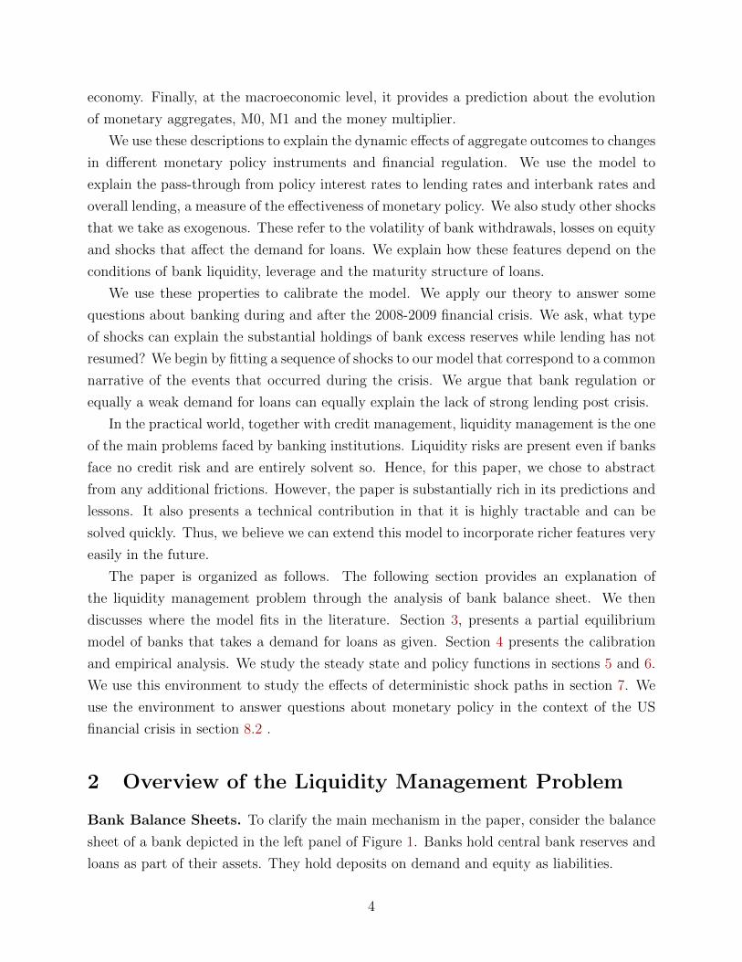
2 Overview of the Liquidity Management Problem

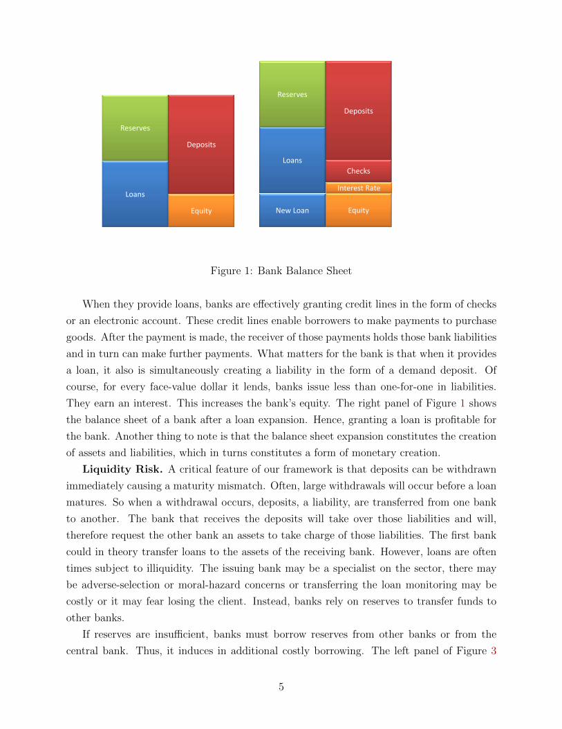
Bank Balance Sheets. To clarify the main mechanism in the paper, consider the balance

sheet of a bank depicted in the left panel of Figure 1. Banks hold central bank reserves and

loans as part of their assets. They hold deposits on demand and equity as liabilities.

4

Reserves

Loans

Deposits

Equity

Reserves

Loans

Deposits

EquityNew Loan

Interest Rate

Checks

Figure 1: Bank Balance Sheet

When they provide loans, banks are effectively granting credit lines in the form of checks

or an electronic account. These credit lines enable borrowers to make payments to purchase

goods. After the payment is made, the receiver of those payments holds those bank liabilities

and in turn can make further payments. What matters for the bank is that when it provides

a loan, it also is simultaneously creating a liability in the form of a demand deposit. Of

course, for every face-value dollar it lends, banks issue less than one-for-one in liabilities.

They earn an interest. This increases the bank’s equity. The right panel of Figure 1 shows

the balance sheet of a bank after a loan expansion. Hence, granting a loan is profitable for

the bank. Another thing to note is that the balance sheet expansion constitutes the creation

of assets and liabilities, which in turns constitutes a form of monetary creation.

Liquidity Risk. A critical feature of our framework is that deposits can be withdrawn

immediately causing a maturity mismatch. Often, large withdrawals will occur before a loan

matures. So when a withdrawal occurs, deposits, a liability, are transferred from one bank

to another. The bank that receives the deposits will take over those liabilities and will,

therefore request the other bank an assets to take charge of those liabilities. The first bank

could in theory transfer loans to the assets of the receiving bank. However, loans are often

times subject to illiquidity. The issuing bank may be a specialist on the sector, there may

be adverse-selection or moral-hazard concerns or transferring the loan monitoring may be

costly or it may fear losing the client. Instead, banks rely on reserves to transfer funds to

other banks.

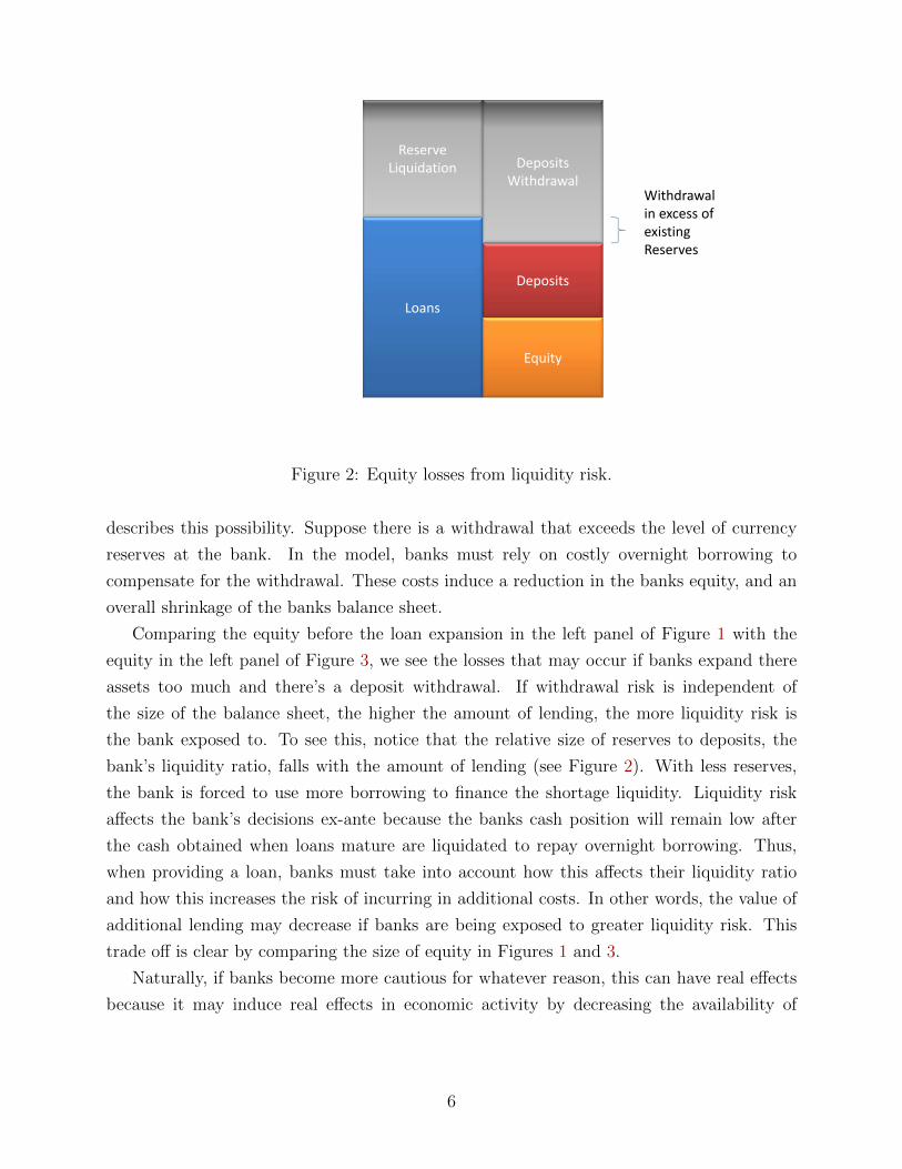
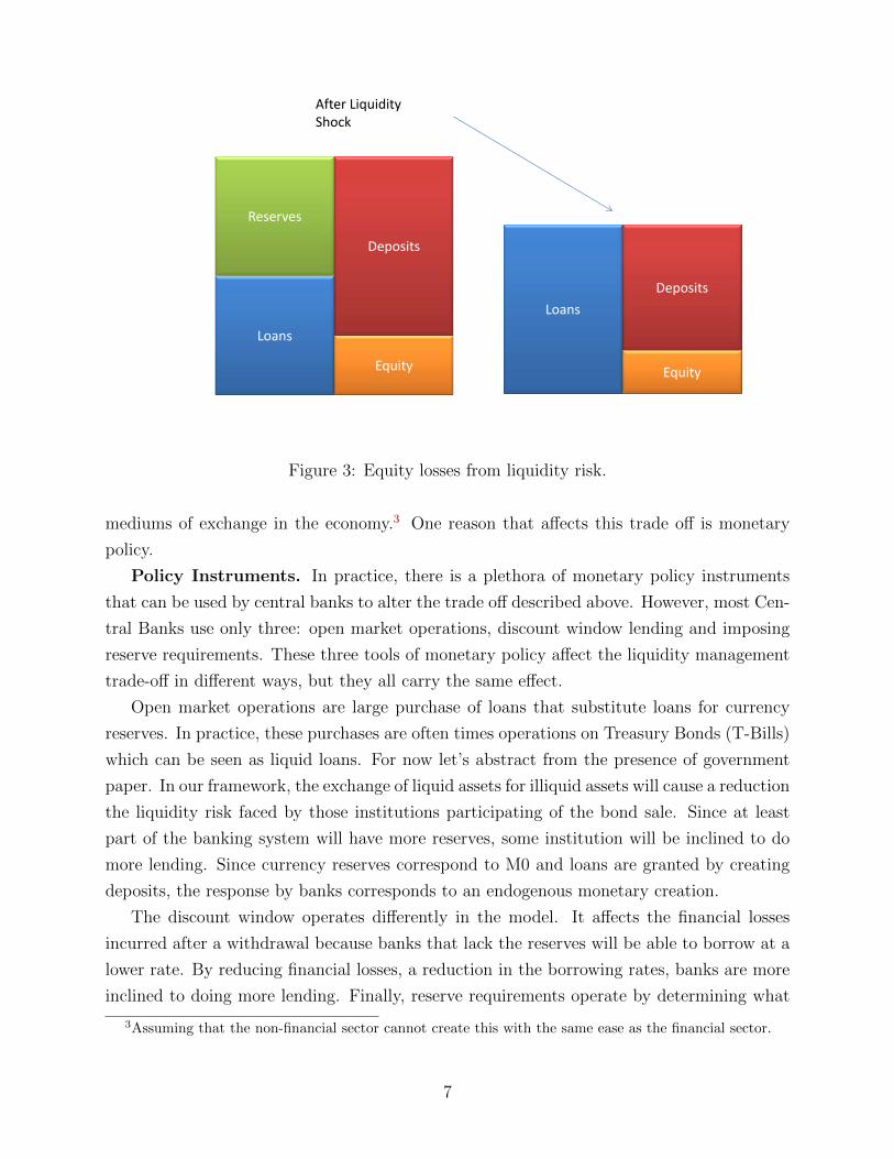
If reserves are insufficient, banks must borrow reserves from other banks or from the

central bank. Thus, it induces in additional costly borrowing. The left panel of Figure 3

5

Loans

Deposits

Equity

DepositsWithdrawal

ReserveLiquidation

Withdrawalin excess of existing Reserves

Figure 2: Equity losses from liquidity risk.

describes this possibility. Suppose there is a withdrawal that exceeds the level of currency

reserves at the bank. In the model, banks must rely on costly overnight borrowing to

compensate for the withdrawal. These costs induce a reduction in the banks equity, and an

overall shrinkage of the banks balance sheet.

Comparing the equity before the loan expansion in the left panel of Figure 1 with the

equity in the left panel of Figure 3, we see the losses that may occur if banks expand there

assets too much and there’s a deposit withdrawal. If withdrawal risk is independent of

the size of the balance sheet, the higher the amount of lending, the more liquidity risk is

the bank exposed to. To see this, notice that the relative size of reserves to deposits, the

bank’s liquidity ratio, falls with the amount of lending (see Figure 2). With less reserves,

the bank is forced to use more borrowing to finance the shortage liquidity. Liquidity risk

affects the bank’s decisions ex-ante because the banks cash position will remain low after

the cash obtained when loans mature are liquidated to repay overnight borrowing. Thus,

when providing a loan, banks must take into account how this affects their liquidity ratio

and how this increases the risk of incurring in additional costs. In other words, the value of

additional lending may decrease if banks are being exposed to greater liquidity risk. This

trade off is clear by comparing the size of equity in Figures 1 and 3.

Naturally, if banks become more cautious for whatever reason, this can have real effects

because it may induce real effects in economic activity by decreasing the availability of

6

Loans

Equity

Deposits

Reserves

Loans

Deposits

Equity

After Liquidity Shock

Figure 3: Equity losses from liquidity risk.

mediums of exchange in the economy.3 One reason that affects this trade off is monetary

policy.

Policy Instruments. In practice, there is a plethora of monetary policy instruments

that can be used by central banks to alter the trade off described above. However, most Cen-

tral Banks use only three: open market operations, discount window lending and imposing

reserve requirements. These three tools of monetary policy affect the liquidity management

trade-off in different ways, but they all carry the same effect.

Open market operations are large purchase of loans that substitute loans for currency

reserves. In practice, these purchases are often times operations on Treasury Bonds (T-Bills)

which can be seen as liquid loans. For now let’s abstract from the presence of government

paper. In our framework, the exchange of liquid assets for illiquid assets will cause a reduction

the liquidity risk faced by those institutions participating of the bond sale. Since at least

part of the banking system will have more reserves, some institution will be inclined to do

more lending. Since currency reserves correspond to M0 and loans are granted by creating

deposits, the response by banks corresponds to an endogenous monetary creation.

The discount window operates differently in the model. It affects the financial losses

incurred after a withdrawal because banks that lack the reserves will be able to borrow at a

lower rate. By reducing financial losses, a reduction in the borrowing rates, banks are more

inclined to doing more lending. Finally, reserve requirements operate by determining what

3Assuming that the non-financial sector cannot create this with the same ease as the financial sector.

7

is the level of currency after which banks have to start borrowing reserves. Penalties on

missing that target are another possible instrument.

2.1 Literature Review

There is a long tradition that dates at least Bagehot (1999) in describing the importance of

banking for the transmission of monetary policy. A first formal attempt to present this in a

model with a full description of households, firms and banks is Gurley and Shaw (1964). The

approach of modeling banks in the implementation of monetary policy was practically aban-

doned from macroeconomics for many years.4 Until the Great Recession, questions of how

monetary policy affects the macroeconomic environment and how it is implemented through

banks were treated independently. This simplification was a natural outcome. Banking

didn’t seem to matter much for the macro-economy in the US. The banking industry was

amongst the most stable industries in terms of dividend ratios, solvency ratios and stock

market value. The pass-through between policy rates and key rates seemed or between the

monetary base and higher aggregates was seen as stable. Moreover, all post-war recessions

in the US have had a name attached to it, but only one of these, the Savings and Loans

crisis, has a name attached to financial system.

In the aftermath of the Great Recession, there has been numerous calls for writing models

with an explicit role for banks in the determination of monetary policy. To name some few

surveys, see for example Woodford (2010) and Mishkin (2011).

The profession has responded rapidly to these calls. We will undoubtedly make an unfair

job of citing the most relevant papers to this one. For example, Gertler and Karadi (2009) and

Curdia and Woodford (2009) study the effects of open market operations in environments

where intermediaries face leverage-like constraints that invest directly in firm’s equity. A

notable distinction of our model is that we introduce a liquidity choice by banks, which

allows us to endogeneize a critical aspect of banks’ risk management. Moreover, this allows

us to study how different shocks and policies affect the financial sector, by altering both

solvency and liquidity positions.

Our paper tries to bring ideas from the banking literature into a fully-fledged dynamic

macro model. In particular we focus on a maturity mismatch problem which leads to a

demand for reserves. The idea is borrowed from the classical papers on banking, (e.g.

Diamond and Dybvig (1983)) which makes banks subject to the risk of withdrawals. Part of

the focus of this literatures is the of study bank runs.5 For us, the maturity mismatch problem

4We are thinking of banking as a subset of models with macroeconomic models with financial frictions,which themselves where few.

5See Gertler and Kiyotaki (2013) for a recent model that incorporates bank runs into DSGE models.

8

simply yields a demand for central bank reserves as a hedging instrument to financial costs

associated with these losses. Along that dimension, we also borrow ideas from the literature

on the payments system in Freeman (1996) and a sequence of other related papers. The

banking payments system leads to liquidity management problem which studied early on by

Frost (1971).

The maturity mismatch problem hence yields a hedging demand for reserves which can

explain how monetary policy effects bank lending. Also recently, Stein (2012) studies an

environment where this demand emerges via an exogenous demand for safe assets in the

utility function but abstracts from dynamics. A related model to ours in focusing on the

dynamics of asset creation by banks is Brunnermeier and Sannikov (2012). They present an

environment where banks create inside money and the central bank creates outside money.

Outside money plays the same role as inside money as a medium of exchange that allows

investment opportunities to be carried out. We share the spirit of having money as an asset

that relaxes constraints but we differ in that outside money are FED reserves which are not

used for commercial transactions. For us, reserves are special for the payments system.

Another paper with a special role for bank assets is Bolton and Freixas (2009). This paper

introduces a differentiated role for different bank liabilities due to asymmetric information.

Prior to the crisis, Stiglitz and Greenwald (2003) suggested the need of an explicit modeling

of banks and asymmetric information problems to understand monetary economics. Stiglitz

and Greenwald (2003) argued that monetary policy can have highly non-linear effects because

of this feature. The demand for loans shocks that we study here have a motivation that is

related with credit rationing. We are far from studying a rich lending problem here but we

hope to head in that direction soon.

A model particularly relevant for us is Afonso and Lagos (2012) who focus on the market

for bank reserves. These authors study the market for FED funds through a money search

environment to explain the allocations and trades the intra-day money markets. We view

are model as the counterpart to theirs in that we study what occurs during the rest of the

day taking as given the outcomes in their marker. A demand for reserve emerges the reserve

position will affect bank payoffs when they enter the Afonso and Lagos (2012) market.

In a sequence of papers, Corbae and D’Erasmo (2013a,b) study the industry dynamics

of the banking industry focusing on the too-big-to-fail advantage by large banks. Our paper

differs from all of this papers in that we stress a liquidity management problem for banks but

we have in common that are models are fully dynamic. We also share common features with

two other papers. The key friction in our model is like in Gertler and Kiyotaki (2012) and

relates to the presence of withdrawal shocks. As them, we share the spirit of the classical

work by Diamond and Dybvig (1983), Allen and Gale (1998) and Holmstrom and Tirole

9

(1997); Holmstrm and Tirole (1998).

Recent empirical papers include the work by Krishnamurthy and Vissing-Jørgensen (2011,

2012). Our model more closely relates to the study of Kashyap and Stein (2000) on the effects

of monetary policy via the lending channel. In fact, we believe we model the credit channel

they refer to. Kashyap and Stein (2012) study the optimality of interests on reserves.

Although not often found in macroeconomics, there are many textbooks on practical

banking that touch the subject. See for example, Saunders and Cornett (2010) or Duttweiler

(2009). Our model can be also seen as a model where withdrawal risk leads to a demand

for reserves. Due to this problem, we break the Modigliani-Miller theorem for open market

operations stressed in Wallace (1981).

3 Partial Equilibrium Model

We begin our description of with a partial equilibrium dynamic model of competing banks.

The focus of this section is on explaining bank decisions as functions of policy variables. In

particular we want to understand the supply of loans function as functions of bank states

and aggregate shocks. We then close the model introducing a real sector which will have a

demand for loans. We choose this organization of our model because there are many ways

of closing the model and we don’t need to impose a particular structure. It turns out that

the way in which we close the model is by imposing assumptions such that monetary policy

has real effects despite that the model is entirely real.

Time is discrete and indexed by t. There is an infinite horizon. Each period is divided

into two stages: a lending stage (l) and a cash-balancing stage (b). A dollar plays the

role of the numeraire. The economy is populated by a continuum of heterogenous banks

whose identity is denoted by z. Banks face an exogenous demand for loans, an exogenous

deterministic monetary policy and a vector of shocks that we describe later.

3.1 Banks

The goal of banks is to maximize dividend payment streams DIVtt≥0 . The bank’s prefer-

ences over dividend streams are evaluated via an expected utility criterion:

E

[∑t≥0

βtU (DIVt)

]

where U (x) ≡ x1−γ

1−γ and DIVt is the banker’s consumption at date t. Banks hold a portfolio

of loans, Bt, and Central Bank reserves, Ct, as part of their assets and demand deposits,

10

Dt, as their liabilities. These are the bank’s individual state variables. We describe some

properties of these state variables.

Loans. When granting a loan, borrowers promise to repay the bank It (1− δ) δn in

period t+n for all n ≥ 0, in units of the numeraire.6 Hence, loans constitute long-run assets

which are a promise to a geometrically decaying stream of payments. Notice that the total

coupon payments that a bank will receive by time t+T from a loan made at t is:

Pt+T = (1− δ) It + (1− δ) Itδ + (1− δ) Itδ2 + .......+ (1− δ) ItδT

so clearly,

limT→∞

Pt+T = It.

The state variable the total coupon payments at time t, which we denote by Bt. Using the

same sequence of payments, total coupon payments received at any point in time are:

Bt = (1− δ)It−1 + (1− δ)δIt−2 + (1− δ)δ2It−3 ......

At t+ 1,

Bt+1 = (1− δ)It + (1− δ)δ2It−1 + (1− δ)δ3It−2 ......

so we can write the law of motion of loans as:

Bt+1 = δBt + (1− δ)It.

Thus, Bt+1, is the value of all future coupon payments including the current ones. Banks

grant new loans It at a market price qt.7 The inverse of this price,

(qlt)−1

is taken as given

and represents the lending rate. In particular, when giving a loan, banks create demand

deposits in the size of the loan qltIt. These deposits are given to the borrower who can use

them to make payments. The rest of the loan, the amount(1− qlt

)It, is a bank’s immediate

profits from intermediation.

An important assumption is that bank loans are illiquid. They can be sold to other banks

but only during the lending stage.8 The underlying assumption is that banks specialize in

6Payments begin at the period of issuance without loss of generality.7This can be easily generalized to allow for some degree of market power. We use the price of the loan

for convenience but one can easily go back and forth from prices to interest rates.8Allowing loans to be sold only during the lending stage is done for convenience. By preventing loans

from being sold during the balancing stage, we introduce a form of illiquidity that is essential to having loansbeing illiquid. Allowing loans to be transferable during the lending stage, is useful to reduce the state spaceof the model. In particular, we will show that it won’t be necessary to keep track of the composition butonly the size of the balance sheet thanks to this assumption.

11

their loans perhaps because they have particular expertise on their borrowers, or specialize

in certain industries. Loans can be also illiquid due to adverse selection. For any of these

reasons, banks would need to spend some time to analyze a loan before buying it. This

assumption can be easily relaxed by allowing sales at a discount at the expense of requiring

one additional state variable.

Finally, we assume there is a clearing house that will allow the bank to reduce its deposit

levels as loans matures. New loans are granted during the lending stage.

Demand Deposits. Behind the scenes, banks have an implicit technology that is en-

abling transactions between third parties. Deposits are created when banks provide loans.

As noted above, when granting loans, the borrower receives a credit line which enables him to

purchase goods. Thus, when providing a new loan, banks are also creating deposits callable

on demand. They are creating an asset (a liability for their borrower) and issuing a liability

(an asset for a third party). The borrower uses these deposits to purchase goods. The holder

of these deposits can, in turn, transfer the funds to others and, so on. Implicitly, bank

deposits are playing a role as a medium of exchange. Simultaneously, banks are liable to the

holder of those deposits.

Demand deposits are the bank’s only form of liability. Deposits are reduced when bor-

rowers make payments to the bank. Essentially, deposits are returned to the bank. Thinking

of the financial system as a whole, it is providing lines of credit so that borrowers can perform

transactions. Eventually, the borrower must obtain back deposits to repay previously issued

loans.

During the balancing stage, banks face a random deposit-withdrawal shock wt. The pro-

cess for the stochastic withdrawals satisfies wt = ωtDt, where ω ∼ F (·, φt) in (−∞, 1]). The

parameter φt is an exogenous process that affects the possible withdrawal risks. When wt

is realized, it decreases the deposits from a bank by that amount. In the background, over

time, these deposits are transferred by there from one bank to another bank. This process

seems a natural process since deposits are being constantly used for transactions. We think

of wt as capturing the complexity of transactions in the payments system which ultimately

lead to randomness in withdrawals.

For the time being, we assume that deposits do not leave the banking sector:

Assumption 1 (Deposit Conservation). Deposits are preserved within the financial sector:∫ ∞0

ωtDtF (dω, φt) = 0, ∀φt

Under the assumption above, we will see, that it is equivalent to saying that there are

no withdrawals of reserves from the banking system or otherwise that there are no runs on

12

the system.9

Since at the balancing stage, we treat bank loans as perfectly illiquid, when a deposit is

transferred from one bank to another, the bank receiving the deposits will request exchange

reserves to clear out the deposit transaction. Thus, reserves are special assets: they are

completely liquid. Banks experience the withdrawal shocks during the lending stage.

Reserves. Banks use reserves to finance the transfer of deposits from one bank to the

other. They often have sufficient reserves to meet there payments but if the shock is very

large (small), reserves may be short (long) of funding the outflow (inflow) of deposits. If so, a

Bank must head to the discount window or the interbank market and pay (earn) an interest

on an short term loan. The cost (benefit) of borrowing (lending) reservers is determined by

the function χ. We interpret χ is a policy parameter that captures a combination of the

discount window and the overnight fed-funds market. They show how the discount window

rate will affect the bank’s discount rate.

Now, the point at which banks are in need of borrowing is not necessarily zero reserves.

In particular, banks may need to borrow if after the withdrawal, they are below a reserve

requirement which is determined by a policy parameter ρ ∈ [0, 1] . Thus, if at any point

ρDt ≥ Ct, bank’s face a penalty χ (ρDt − Ct) in the form of borrowing needs.

The function χ maps deviation from reserve requirements to a penalty:

χ(x) =

χx if x ≤ 0

χx if x > 0.

An important parameter restriction is that χ < χ. In practice, central banks set up

windows for lending and borrowing rates overnight. Afonso and Lagos (2012) provide a

formal model for the overnight interbank market. The outcome of their analysis is that

banks ending a day with positive balances lend out reserves to banks with negative balances

with a certain probability. The balance that is not lend earns interest on deposits at the FED

and the fraction that cannot be borrowed pays interests.10 Our interpretationχ, χ

is as an

average of repeated interactions in the FED funds market. The values forχ, χ

represent

the average cost of ending with positive or negative balances considering that banks can

borrow from the interbank market with a certain probability or otherwise they must lend or

borrow from the FED. We takeχ, χ

as policy parameters.

9We can extend the model easily assuming that the private sector can withdraw deposits in the form ofcurrency. This can be easily incorporated disposing the assumption that deposits do not leave the bankingsector.

10We can extend our model by allowing the opening of this market with possible interesting interactions.

13

Bank Equity. Bank equity is the sum of their assets minus their liabilities:

Nt = Bt + Ct −Dt

Equity evolves according to the realization of bank profits that stem from lending to

customers and borrowing from the interbank market. Profits are realized during the lending

stage. Also, during the lending stage, part of the bank’s equity can be payed-out as dividends,

DIVt. Dividends are payed-out by issuing deposits to bank share holders. Finally, banks face

a regulatory framework that constraints the amount of loans they can make and dividends

they can payout.

3.2 Timing of Events and Laws of Motion

Notation. We use Zt to denote the value of variable Zt during the lending stage and Zt to

denote its value at the beginning of the rebalancing stage.

Lending Stage: Banks enter the period during the lending stage with currency Ct, a

portfolio of loans Bt, and a deposits, Dt as their individual states. The aggregate state

includes monetary policy variables (for now treated as parameters), real economic activity

observables (for now constant), and an exogenous demand for loans (for now exogenous).

This aggregate states are summarized in the vector Xt.

During the lending stage, banks decide over the amount of new loans they provide, It,

dividend payments DIVt and, ϕt, their purchases of reserves. These interbank transactions,

ϕt, occur during the lending stage so they are different from the overnight FED-funds market

that cost χ. This borrowing occur at an interest rate of r so we think of these as the LIBOR

rate. This interest is payed in the form of deposits.

Upon a loan banks give a checking account to the borrower, or equivalently a deposit

account to whom ever is exchanging a physical good (resources) to the borrower (in exchange

for that check). When borrowing (lending) reserves, they issue (are issued) deposits against

those assets. Thus, since dividends are payed in the form of bank liabilities, we obtain the

following intra-period law of motion for demand deposits:

Dt = Dt + qIt +DIVt + ϕt(1 + rt)−Bt(1− δ). (1)

Thus, a bank that begins with Dt as deposits at the beginning of the stage ends with Dt

at the end through the following sources. It credits by qIt the account of his borrower (or

whomever he trades with), after a loan of size It. It also pays dividends to shareholders in

amount DIVt. It issues ϕt(1 + rt) liabilities to other banks if it borrows ϕt in cash. Finally,

14

−Bt(1− δ) deposits are reduced by the payment of previously issued loans.

The evolution of bank reserves is given by the sum of the previous stock plus the interest

on reserves (rcCt) plus the cash purchases,

Ct = (1 + rc)Ct + ϕt. (2)

Interests on reserves rc, are payed by the monetary authority in the form of more reserves.

Finally, loans evolve according to the fraction of the original stock that has not matured yet

plus the newly issued loans.

Bt = δBt + It. (3)

Banks make these choices subject to the following capital requirement constraint that

puts an upper bound on the amount of leverage the bank can take

Dt ≤ κNt, (4)

and to a liquidity requirement,

Ct ≥ ηNt (5)

which differs from the monetary policy reserve requirement.

Balancing Stage. During the balancing stage, banks receive the random deposit with-

drawal shock ωt. This shock is like a random increase in the demand for cash. If by the end

of the period, banks do not hold sufficient cash relative to the deposits, they face penalties

χ(ρDt − Ct). Penalties are payed in the form of deposits.

Hence the law of motion for cash accounts for the withdrawal,

Ct+1 = Ct − ωtDt

and

Dt+1 = Dt(1− ωt) + χ(ρDt − Ct)).

That is, cash at the end of the period are given, by cash selected at the beginning of the

period minus withdrawn deposits at the end of the period. The second law of motion reflects

the liquidity shock and the fact that the penalty χ is repaid with deposits.

3.3 Bank Problems

The model can be expressed recursively so for its statement, we drop time subscripts. It is

understood that prices (q, r) and policy variables(κ, η, rc,

χ, χ

)as well as the distribution

15

of shocks F are functions of the aggregate state X.

Lending Stage. The optimization problem for a bank during the lending stage in

recursive form is as follows.

Problem 1 (Bank Lending Stage) The bank’s problem during the lending stage is:

V l(C,B,D;X) = maxI,DIV,ϕ∈R

U (DIV ) + E[V b(C, B, D; X)

]D = D + qI +DIV + ϕ(1 + r)−B(1− δ)

C = C (1 + rc) + ϕ

B′ = δB + I

D ≤ κ(B + C − D), D ≥ 0

C ≥ η(B + C − D), C ≥ 0

Banks choose loans I, dividends DIV, reserve holdings C and deposits D to maximize

expected dividends. The solve this problem subject to the law’s of motions for deposits,

reserves and loans, equations (1), 2 and (3). In addition, they must satisfy the policy

constraints (4) and (5). On the technical side, the leverage constraints bounds the problem

of the banks and thus renders their problem feasible. It prevents a Ponzi-scheme. Moreover,

since D ≥ 0, equity will remain positive at all periods before the ω shock is realized.

It is important to note that if the bank arrives to a node with negative equity, the problem

is not well defined. However, in choosing its policies, it will make decisions such that it is

guaranteed that it doesn’t run out of equity.

During the balancing state, banks make no decisions but rather experience the withdrawal

shock ω. There problem is given by the following condition:

Problem 2 (Bank Balancing Stage) The bank’s problem during the balancing stage is:

V b(C, B, D; X) = βE[V l(C ′, B′, D′;X ′)|X

]C ′ = C − ωD

B′ = B

D′ = D(1− ω) + χ(ρD − C ′)

Loans remain unchanged as withdrawals do not affect the stock of loans. Instead, ωD

are transferred to other banks in the form of reserves. The withdrawal reduces deposits

by (1 − ω). Finally, deposits change depending on the penalty faced by banks χ. We can

collapse the model into a single period. Since there are no actions between periods, then

16

there’s no need to write-up two Bellman equations. Combining the lending and balancing

stage problems we obtain a value function for the balancing stage which is recursive:

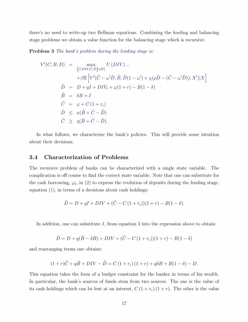
Problem 3 The bank’s problem during the lending stage is:

V l(C,B,D) = maxI,DIV,C,D∈R4

+

U (DIV ) ...

+βE[V l(C − ω′D, B, D(1− ω′) + χ(ρD − (C − ω′D));X ′)|X

]D = D + qI +DIVt + ϕ(1 + r)−B(1− δ)

B = δB + I

C = ϕ+ C (1 + rc)

D ≤ κ(B + C − D)

C ≥ η(B + C − D).

In what follows, we characterize the bank’s policies. This will provide some intuition

about their decisions.

3.4 Characterization of Problems

The recursive problem of banks can be characterized with a single state variable. The

complication is off course to find the correct state variable. Note that one can substitute for

the cash borrowing, ϕt, in (2) to express the evolution of deposits during the lending stage,

equation (1), in terms of a decisions about cash holdings:

D = D + qI +DIV + (C − C (1 + rc))(1 + r)−B(1− δ).

In addition, one can substitute I, from equation 3 into the expression above to obtain:

D = D + q(B − δB) +DIV + (C − C (1 + rc))(1 + r)−B(1− δ)

and rearranging terms one obtains:

(1 + r)C + qB +DIV − D = C (1 + rc) (1 + r) + qδB +B(1− δ)−D.

This equation takes the form of a budget constraint for the banker in terms of his wealth.

In particular, the bank’s sources of funds stem from two sources. The one is the value of

its cash holdings which can be lent at an interest, C (1 + rc) (1 + r). The other is the value

17

of loans. The illiquid fraction of loans, δB, is valued at q because this is the replacement

cost of the illiquid fraction. The rest, B(1 − δ), is valued at the same amount as deposits.

Deposits are subtracted from the bank’s total loans. Funds are used to obtain cash for the

following period, C, to fund new loans B or to pay dividends, DIV. Naturally, these uses

can be expanded by issuing more liabilities, D today.

One can define the market value of equity as, E ≡ C (1 + rc) (1+r)+qδB+B(1−δ)−D,corresponding to the right hand side of the bank’s budget constraint. If we ignore the

constraints that B ≥ δB, something that can be ruled in equilibrium, we can express the

Bellman equation without reference to the different states but only as a function of E. Thus,

Proposition 1 (Single-State Representation) The problem of the bank can be written the

following way:

V l(E) = maxC,B′,D,DIV ∈R4

+

u(DIV ) + βE[V l(E ′)|X

]E = qB + C(1 + r) +DIV − D

E ′ = (q′δ + (1− δ)) B + C (1 + rc) (1 + r′)− D(1 + (1 + rc) r′ω′)− χ((ρ+ ω) D − C))

D ≤ κ(B + C − D)

C ≥ η(B + C − D)

The first constraint now collapse all of the laws of motion for the bank’s assets. It now

writes them as a budget constraint in term’s of the bank’s equity (wealth). This is a familiar

budget constraint in that the bank must choose consumption, or dividends, and two assets,(B, C

)and borrowing D subject to a leverage constraint and liquidity constraint. He then

makes this decision to maximize utility taking into account the law of motion for his equity

after the liquidity shock.11

The continuation value of the value function, has also one argument, E ′, which is ob-

tained by substituting the values of D’,C’ and B’ as functions of current states. The budget

constraint is linear in E and the objective is homothetic in dividends. Thus, by Alvarez and

Stokey (1998) we have that the solution to this problem exists and is unique and we have

that policy functions are linear.

One can guess and verify that the objective is:

Proposition 2 (Homogeneity-γ) The value function V l(E;X) satisfies

V l(E;X) = vl (X)E1−γ

11With obvious abuse of notation, V henceforth denotes the value function in terms of E rather than(C,B,D).

18

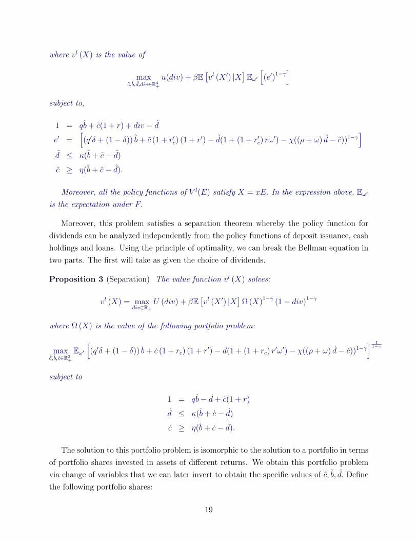
where vl (X) is the value of

maxc,b,d,div∈R4

+

u(div) + βE[vl (X ′) |X

]Eω′[(e′)

1−γ]

subject to,

1 = qb+ c(1 + r) + div − d

e′ =[(q′δ + (1− δ)) b+ c (1 + r′c) (1 + r′)− d(1 + (1 + r′c) rω

′)− χ((ρ+ ω) d− c))1−γ]

d ≤ κ(b+ c− d)

c ≥ η(b+ c− d).

Moreover, all the policy functions of V l(E) satisfy X = xE. In the expression above, Eω′is the expectation under F.

Moreover, this problem satisfies a separation theorem whereby the policy function for

dividends can be analyzed independently from the policy functions of deposit issuance, cash

holdings and loans. Using the principle of optimality, we can break the Bellman equation in

two parts. The first will take as given the choice of dividends.

Proposition 3 (Separation) The value function vl (X) solves:

vl (X) = maxdiv∈R+

U (div) + βE[vl (X ′) |X

]Ω (X)1−γ (1− div)1−γ

where Ω (X) is the value of the following portfolio problem:

maxδ,b,c∈R3

+

Eω′[(q′δ + (1− δ)) b+ c (1 + rc) (1 + r′)− d(1 + (1 + rc) r

′ω′)− χ((ρ+ ω) d− c))1−γ] 1

1−γ

subject to

1 = qb− d+ c(1 + r)

d ≤ κ(b+ c− d)

c ≥ η(b+ c− d).

The solution to this portfolio problem is isomorphic to the solution to a portfolio in terms

of portfolio shares invested in assets of different returns. We obtain this portfolio problem

via change of variables that we can later invert to obtain the specific values of c, b, d. Define

the following portfolio shares:

19

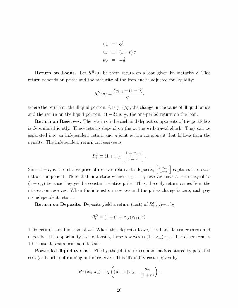
wb ≡ qb

wc ≡ (1 + r) c

wd ≡ −d.

Return on Loans. Let RB (δ) be there return on a loan given its maturity δ. This

return depends on prices and the maturity of the loan and is adjusted for liquidity:

RBt (δ) ≡ δqt+1 + (1− δ)

qt,

where the return on the illiquid portion, δ, is qt+1/qt, the change in the value of illiquid bonds

and the return on the liquid portion. (1− δ) is 1qt, the one-period return on the loan.

Return on Reserves. The return on the cash and deposit components of the portfolios

is determined jointly. These returns depend on the ω, the withdrawal shock. They can be

separated into an independent return and a joint return component that follows from the

penalty. The independent return on reserves is

RCt ≡ (1 + rc,t)

[1 + rt+1

1 + rt

].

Since 1 + rt is the relative price of reserves relative to deposits,[

1+rt+1

1+rt

]captures the reval-

uation component. Note that in a state where rt+1 = rt, reserves have a return equal to

(1 + rc,t) because they yield a constant relative price. Thus, the only return comes from the

interest on reserves. When the interest on reserves and the prices change is zero, cash pay

no independent return.

Return on Deposits. Deposits yield a return (cost) of RDt , given by

RDt ≡ (1 + (1 + rc,t) rt+1ω

′).

This returns are function of ω′. When this deposits leave, the bank losses reserves and

deposits. The opportunity cost of loosing those reserves is (1 + rc,t) rt+1. The other term is

1 because deposits bear no interest.

Portfolio Illiquidity Cost. Finally, the joint return component is captured by potential

cost (or benefit) of running out of reserves. This illiquidity cost is given by,

Rχ (wd, wc) ≡ χ

((ρ+ ω)wd −

wc(1 + r)

).

20

In this expression, (ρ+ ω) is the sum of the reserve requirement and the withdrawal frac-

tion. The cost the actual amount of cash holdings for the bank are (wc/1 + r), the pre-

transformation amount of cash. So when the withdrawal and reserves are lower than the

amount of cash, the agent has a negative account at the fed which activates the borrowing

costs.

Portfolio Problem. Using the returns on the banks assets, we obtain the following

liquidity management portfolio problem:

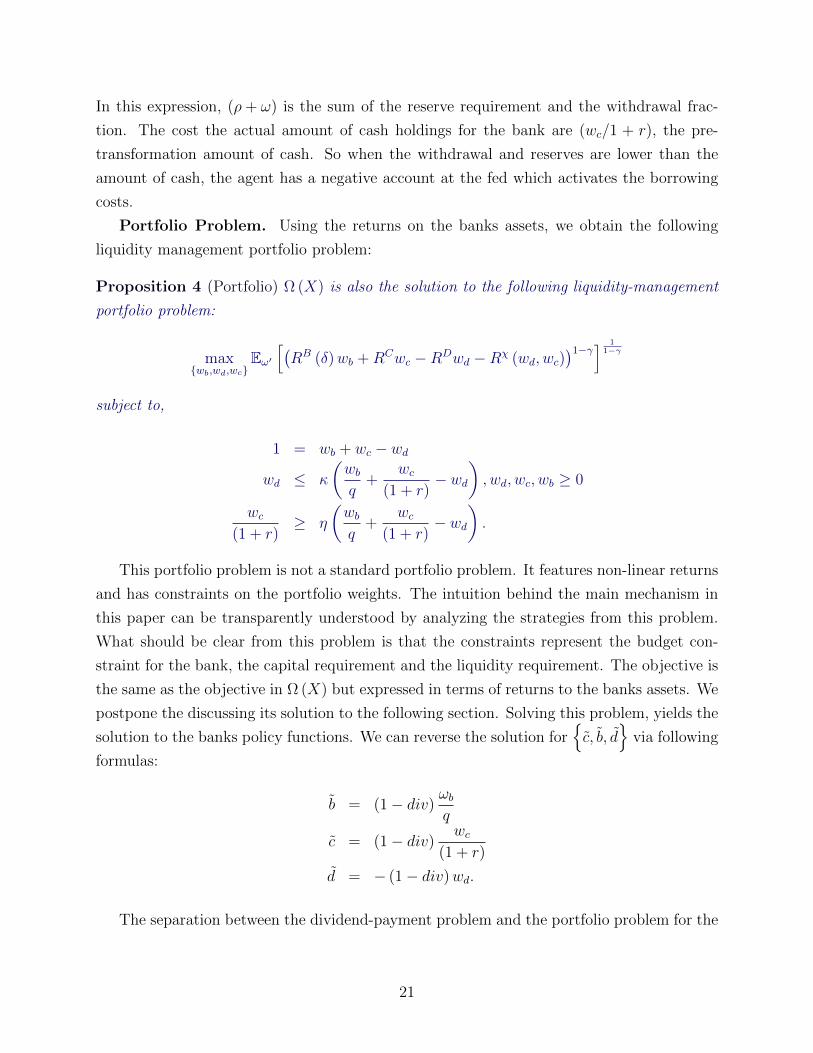
Proposition 4 (Portfolio) Ω (X) is also the solution to the following liquidity-management

portfolio problem:

maxwb,wd,wc

Eω′[(RB (δ)wb +RCwc −RDwd −Rχ (wd, wc)

)1−γ] 1

1−γ

subject to,

1 = wb + wc − wd

wd ≤ κ

(wbq

+wc

(1 + r)− wd

), wd, wc, wb ≥ 0

wc(1 + r)

≥ η

(wbq

+wc

(1 + r)− wd

).

This portfolio problem is not a standard portfolio problem. It features non-linear returns

and has constraints on the portfolio weights. The intuition behind the main mechanism in

this paper can be transparently understood by analyzing the strategies from this problem.

What should be clear from this problem is that the constraints represent the budget con-

straint for the bank, the capital requirement and the liquidity requirement. The objective is

the same as the objective in Ω (X) but expressed in terms of returns to the banks assets. We

postpone the discussing its solution to the following section. Solving this problem, yields the

solution to the banks policy functions. We can reverse the solution forc, b, d

via following

formulas:

b = (1− div)ωbq

c = (1− div)wc

(1 + r)

d = − (1− div)wd.

The separation between the dividend-payment problem and the portfolio problem for the

21

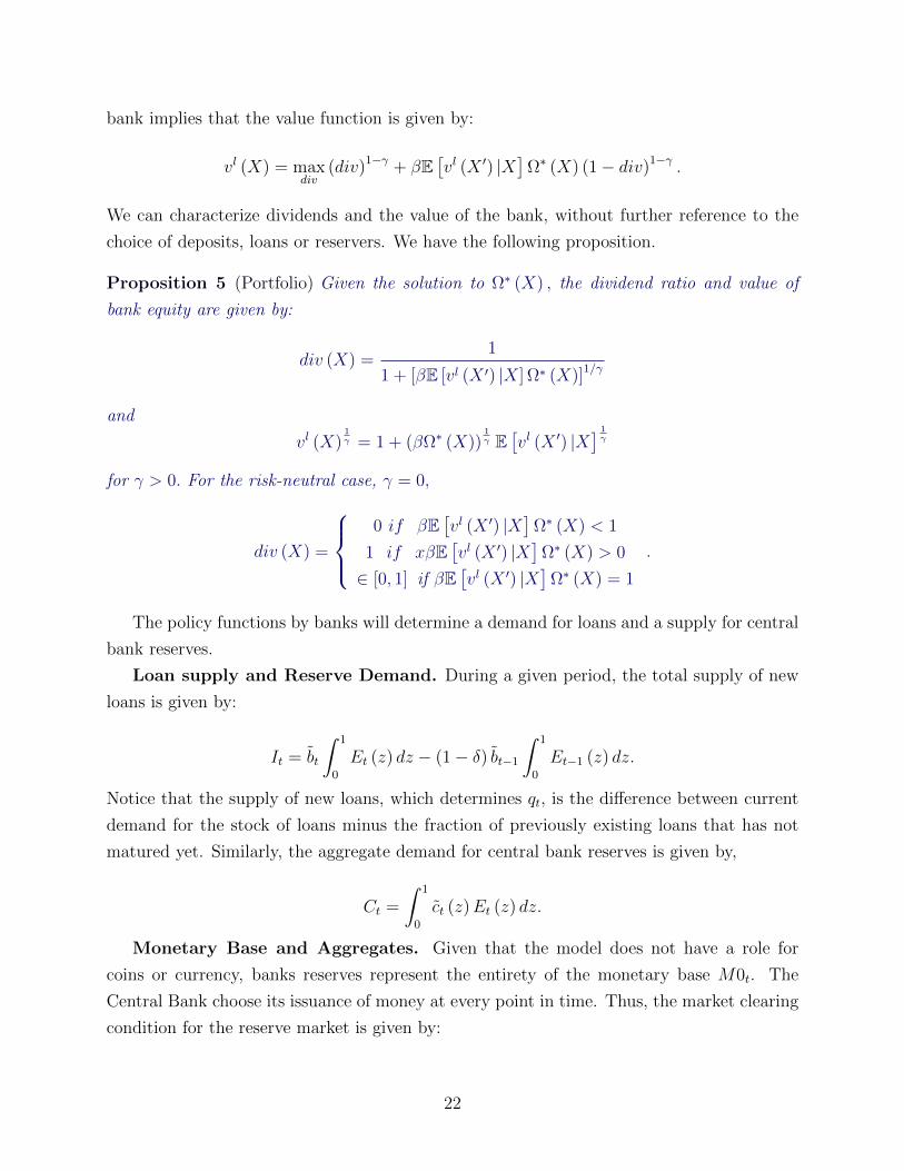
bank implies that the value function is given by:

vl (X) = maxdiv

(div)1−γ + βE[vl (X ′) |X

]Ω∗ (X) (1− div)1−γ .

We can characterize dividends and the value of the bank, without further reference to the

choice of deposits, loans or reservers. We have the following proposition.

Proposition 5 (Portfolio) Given the solution to Ω∗ (X) , the dividend ratio and value of

bank equity are given by:

div (X) =1

1 + [βE [vl (X ′) |X] Ω∗ (X)]1/γ

and

vl (X)1γ = 1 + (βΩ∗ (X))

1γ E[vl (X ′) |X

] 1γ

for γ > 0. For the risk-neutral case, γ = 0,

div (X) =

0 if βE

[vl (X ′) |X

]Ω∗ (X) < 1

1 if xβE[vl (X ′) |X

]Ω∗ (X) > 0

∈ [0, 1] if βE[vl (X ′) |X

]Ω∗ (X) = 1

.

The policy functions by banks will determine a demand for loans and a supply for central

bank reserves.

Loan supply and Reserve Demand. During a given period, the total supply of new

loans is given by:

It = bt

∫ 1

0

Et (z) dz − (1− δ) bt−1

∫ 1

0

Et−1 (z) dz.

Notice that the supply of new loans, which determines qt, is the difference between current

demand for the stock of loans minus the fraction of previously existing loans that has not

matured yet. Similarly, the aggregate demand for central bank reserves is given by,

Ct =

∫ 1

0

ct (z)Et (z) dz.

Monetary Base and Aggregates. Given that the model does not have a role for

coins or currency, banks reserves represent the entirety of the monetary base M0t. The

Central Bank choose its issuance of money at every point in time. Thus, the market clearing

condition for the reserve market is given by:

22

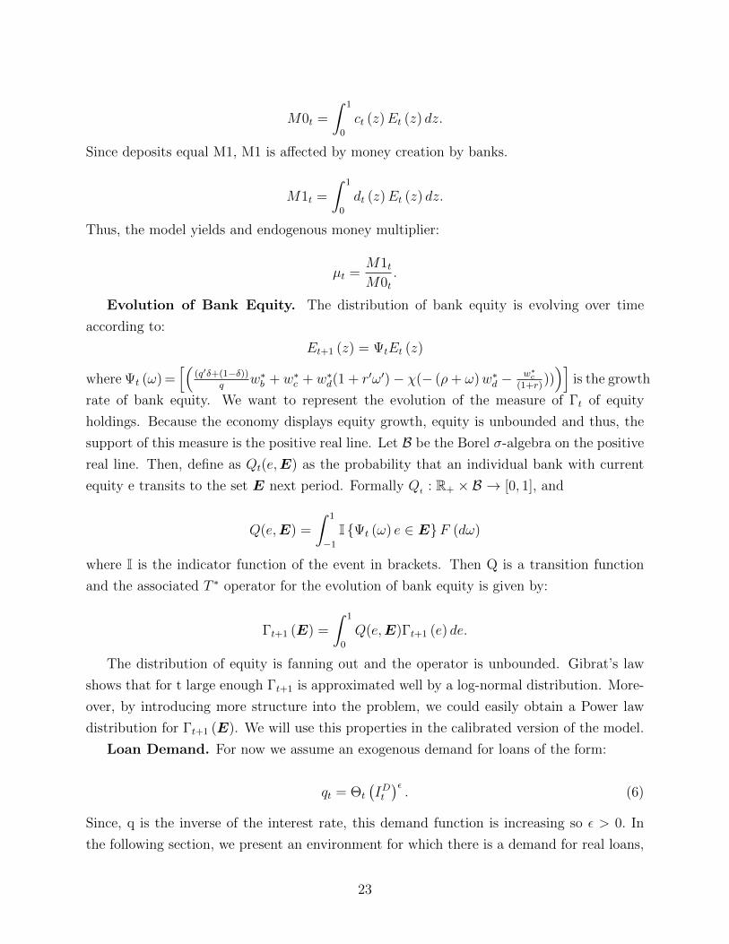
M0t =

∫ 1

0

ct (z)Et (z) dz.

Since deposits equal M1, M1 is affected by money creation by banks.

M1t =

∫ 1

0

dt (z)Et (z) dz.

Thus, the model yields and endogenous money multiplier:

µt =M1tM0t

.

Evolution of Bank Equity. The distribution of bank equity is evolving over time

according to:

Et+1 (z) = ΨtEt (z)

where Ψt (ω) =[(

(q′δ+(1−δ))q

w∗b + w∗c + w∗d(1 + r′ω′)− χ(− (ρ+ ω)w∗d −w∗c

(1+r))))]

is the growth

rate of bank equity. We want to represent the evolution of the measure of Γt of equity

holdings. Because the economy displays equity growth, equity is unbounded and thus, the

support of this measure is the positive real line. Let B be the Borel σ-algebra on the positive

real line. Then, define as Qt(e,E) as the probability that an individual bank with current

equity e transits to the set E next period. Formally Qt : R+ × B → [0, 1], and

Q(e,E) =

∫ 1

−1

I Ψt (ω) e ∈ EF (dω)

where I is the indicator function of the event in brackets. Then Q is a transition function

and the associated T ∗ operator for the evolution of bank equity is given by:

Γt+1 (E) =

∫ 1

0

Q(e,E)Γt+1 (e) de.

The distribution of equity is fanning out and the operator is unbounded. Gibrat’s law

shows that for t large enough Γt+1 is approximated well by a log-normal distribution. More-

over, by introducing more structure into the problem, we could easily obtain a Power law

distribution for Γt+1 (E). We will use this properties in the calibrated version of the model.

Loan Demand. For now we assume an exogenous demand for loans of the form:

qt = Θt

(IDt)ε. (6)

Since, q is the inverse of the interest rate, this demand function is increasing so ε > 0. In

the following section, we present an environment for which there is a demand for real loans,

23

we stems from properly micro-founded models.

In the appendix, we provide a microfoundation for the loan demand 6 that closes the

model.

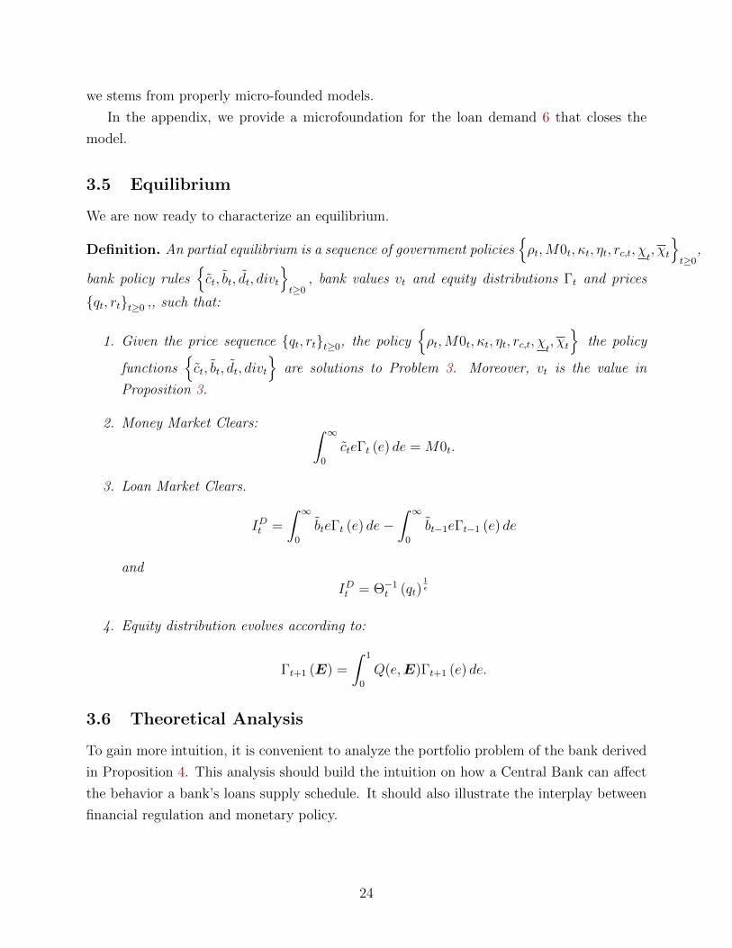
3.5 Equilibrium

We are now ready to characterize an equilibrium.

Definition. An partial equilibrium is a sequence of government policiesρt,M0t, κt, ηt, rc,t, χt, χt

t≥0

,

bank policy rulesct, bt, dt, divt

t≥0

, bank values vt and equity distributions Γt and prices

qt, rtt≥0 ,, such that:

1. Given the price sequence qt, rtt≥0, the policyρt,M0t, κt, ηt, rc,t, χt, χt

the policy

functionsct, bt, dt, divt

are solutions to Problem 3. Moreover, vt is the value in

Proposition 3.

2. Money Market Clears: ∫ ∞0

cteΓt (e) de = M0t.

3. Loan Market Clears.

IDt =

∫ ∞0

bteΓt (e) de−∫ ∞

0

bt−1eΓt−1 (e) de

and

IDt = Θ−1t (qt)

1ε

4. Equity distribution evolves according to:

Γt+1 (E) =

∫ 1

0

Q(e,E)Γt+1 (e) de.

3.6 Theoretical Analysis

To gain more intuition, it is convenient to analyze the portfolio problem of the bank derived

in Proposition 4. This analysis should build the intuition on how a Central Bank can affect

the behavior a bank’s loans supply schedule. It should also illustrate the interplay between

financial regulation and monetary policy.

24

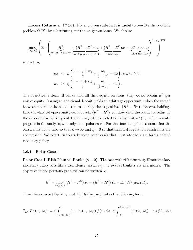
Excess Returns in Ω∗ (X). Fix any given state X. It is useful to re-write the portfolio

problem Ω (X) by substituting out the weight on loans. We obtain:

maxwd,wc

Eω′

RB︸︷︷︸Return to Equity

−(RB −RC

)wc︸ ︷︷ ︸

Cash Opportunity Cost

+(RB −RD

)︸ ︷︷ ︸Arbitrage

wd −Rχ (wd, wc)︸ ︷︷ ︸Liquidity Cost

1−γ

11−γ

subject to,

wd ≤ κ

(1− wc + wd

q+

wc(1 + r)

− wd), wd, wc ≥ 0

wc ≥ η

(1− wc + wd

q+

wc(1 + r)

− wd).

The objective is clear. If banks hold all their equity on loans, they would obtain RB per

unit of equity. Issuing an additional deposit yields an arbitrage opportunity when the spread

between return on loans and return on deposits is positive:(RB −RD

). Reserve holdings

have the classical opportunity cost of cash,(RB −RC

)but they yield the benefit of reducing

the exposure to liquidity risk by reducing the expected liquidity cost Rχ (wd, wc) . To make

progress in the analysis, we study some polar cases. For the time being, let’s assume that the

constraints don’t bind so that κ→∞ and η = 0 so that financial regulation constraints are

not present. We now turn to study some polar cases that illustrate the main forces behind

monetary policy.

3.6.1 Polar Cases

Polar Case I: Risk-Neutral Banks (γ = 0). The case with risk neutrality illustrates how

monetary policy acts like a tax. Hence, assume γ = 0 so that bankers are risk neutral. The

objective in the portfolio problem can be written as:

RB + maxwd,wc

(RB −RD

)wd −

(RB −RC

)wc − Eω′ [Rχ (wd, wc)] .

Then the expected liquidity cost Eω′ [Rχ (wd, wc)] takes the following form:

Eω′ [Rχ (wd, wc)] = χ

∫ 1

ω(wd,wc)

(ω − ω (wd, wc)) f (ω) dω−χ∫ ω(wd,wc)

−∞(ω (wd, wc)− ω) f (ω) dω.

25

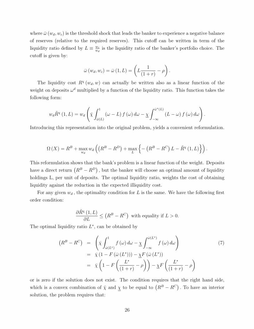
where ω (wd, wc) is the threshold shock that leads the banker to experience a negative balance

of reserves (relative to the required reserves). This cutoff can be written in term of the

liquidity ratio defined by L ≡ wcwd

is the liquidity ratio of the banker’s portfolio choice. The

cutoff is given by:

ω (wd, wc) = ω (1, L) =

(L

1

(1 + r)− ρ).

The liquidity cost Rχ (wd, w) can actually be written also as a linear function of the

weight on deposits ωd multiplied by a function of the liquidity ratio. This function takes the

following form:

wdRχ (1, L) = wd

(χ

∫ 1

ω(L)

(ω − L) f (ω) dω − χ∫ ω∗(L)

−∞(L− ω) f (ω) dω

).

Introducing this representation into the original problem, yields a convenient reformulation.

Ω (X) = RB + maxwd

wd

((RB −RD

)+ max

L

−(RB −RC

)L− Rχ (1, L)

).

This reformulation shows that the bank’s problem is a linear function of the weight. Deposits

have a direct return(RB −RD

), but the banker will choose an optimal amount of liquidity

holdings L, per unit of deposits. The optimal liquidity ratio, weights the cost of obtaining

liquidity against the reduction in the expected illiquidity cost.

For any given wd , the optimality condition for L is the same. We have the following first

order condition:

∂Rχ (1, L)

∂L≤(RB −RC

)with equality if L > 0.

The optimal liquidity ratio L∗, can be obtained by

(RB −RC

)=

(χ

∫ 1

ω(L∗)

f (ω) dω − χ∫ ω(L∗)

−∞f (ω) dω

)(7)

= χ (1− F (ω (L∗)))− χF (ω (L∗))

= χ

(1− F

(L∗

(1 + r)− ρ))− χF

(L∗

(1 + r)− ρ)

or is zero if the solution does not exist. The condition requires that the right hand side,

which is a convex combination of χ and χ to be equal to(RB −RC

). To have an interior

solution, the problem requires that:

26

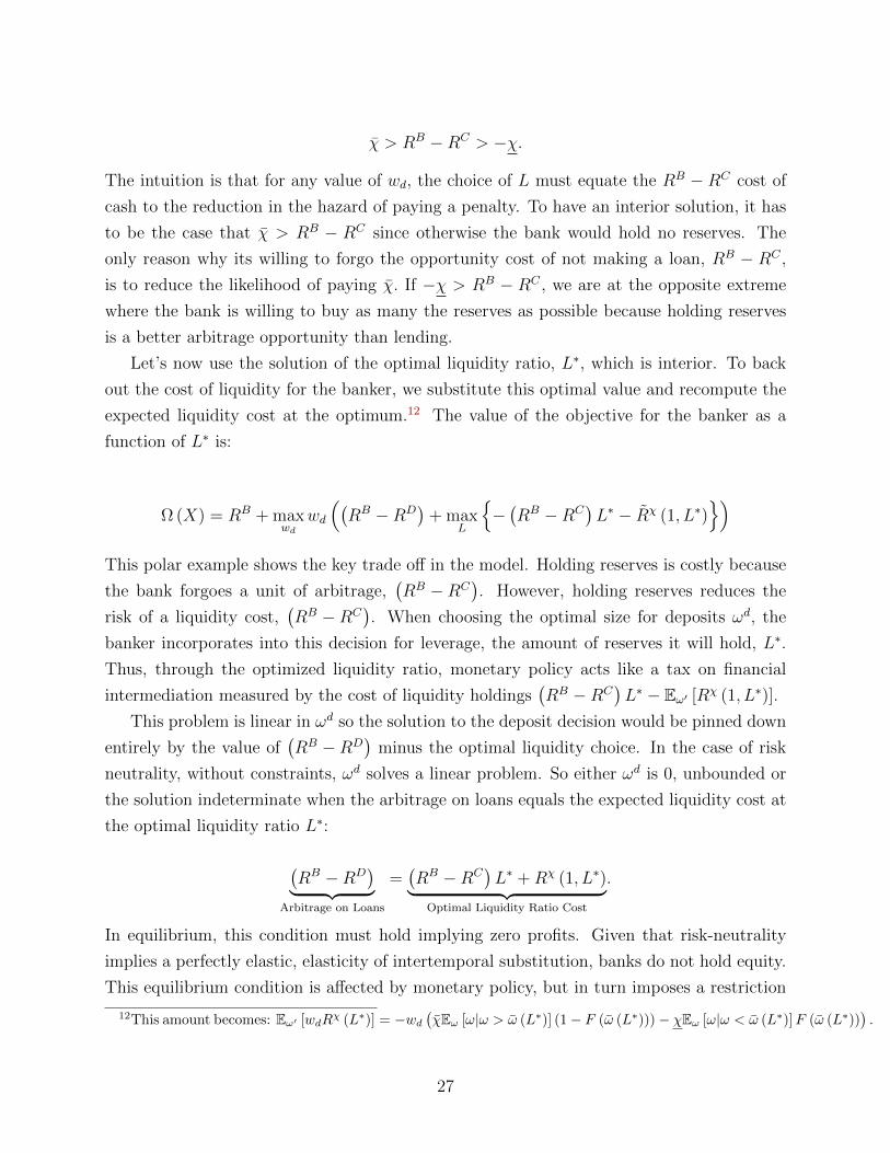
χ > RB −RC > −χ.

The intuition is that for any value of wd, the choice of L must equate the RB − RC cost of

cash to the reduction in the hazard of paying a penalty. To have an interior solution, it has

to be the case that χ > RB − RC since otherwise the bank would hold no reserves. The

only reason why its willing to forgo the opportunity cost of not making a loan, RB − RC ,

is to reduce the likelihood of paying χ. If −χ > RB − RC , we are at the opposite extreme

where the bank is willing to buy as many the reserves as possible because holding reserves

is a better arbitrage opportunity than lending.

Let’s now use the solution of the optimal liquidity ratio, L∗, which is interior. To back

out the cost of liquidity for the banker, we substitute this optimal value and recompute the

expected liquidity cost at the optimum.12 The value of the objective for the banker as a

function of L∗ is:

Ω (X) = RB + maxwd

wd

((RB −RD

)+ max

L

−(RB −RC

)L∗ − Rχ (1, L∗)

)This polar example shows the key trade off in the model. Holding reserves is costly because

the bank forgoes a unit of arbitrage,(RB −RC

). However, holding reserves reduces the

risk of a liquidity cost,(RB −RC

). When choosing the optimal size for deposits ωd, the

banker incorporates into this decision for leverage, the amount of reserves it will hold, L∗.

Thus, through the optimized liquidity ratio, monetary policy acts like a tax on financial

intermediation measured by the cost of liquidity holdings(RB −RC

)L∗ − Eω′ [Rχ (1, L∗)].

This problem is linear in ωd so the solution to the deposit decision would be pinned down

entirely by the value of(RB −RD

)minus the optimal liquidity choice. In the case of risk

neutrality, without constraints, ωd solves a linear problem. So either ωd is 0, unbounded or

the solution indeterminate when the arbitrage on loans equals the expected liquidity cost at

the optimal liquidity ratio L∗:

(RB −RD

)︸ ︷︷ ︸Arbitrage on Loans

=(RB −RC

)L∗ +Rχ (1, L∗)︸ ︷︷ ︸

Optimal Liquidity Ratio Cost

.

In equilibrium, this condition must hold implying zero profits. Given that risk-neutrality

implies a perfectly elastic, elasticity of intertemporal substitution, banks do not hold equity.

This equilibrium condition is affected by monetary policy, but in turn imposes a restriction

12This amount becomes: Eω′ [wdRχ (L∗)] = −wd

(χEω [ω|ω > ω (L∗)] (1− F (ω (L∗)))− χEω [ω|ω < ω (L∗)]F (ω (L∗))

).

27

on the set of equilibria imposed by monetary policy. Two additional polar cases lead to the

very similar constraints.

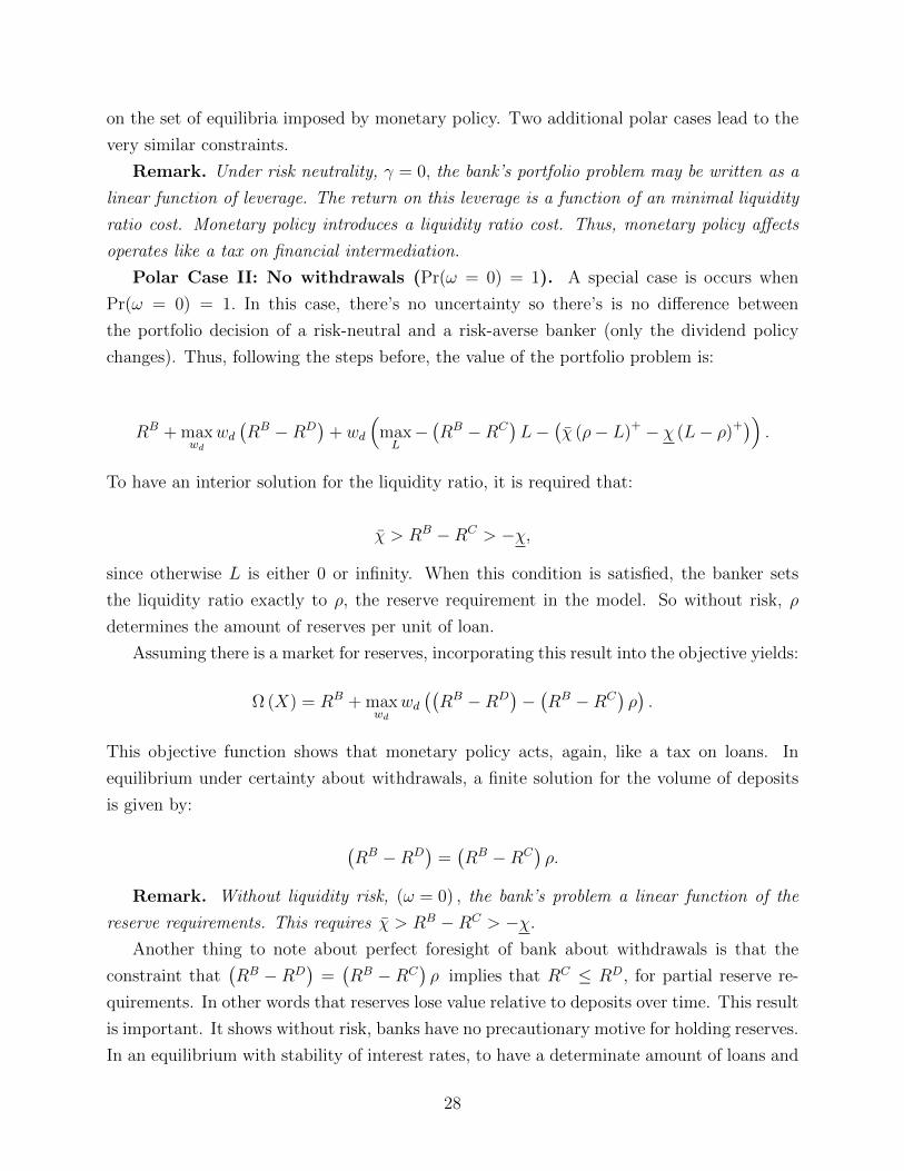
Remark. Under risk neutrality, γ = 0, the bank’s portfolio problem may be written as a

linear function of leverage. The return on this leverage is a function of an minimal liquidity

ratio cost. Monetary policy introduces a liquidity ratio cost. Thus, monetary policy affects

operates like a tax on financial intermediation.

Polar Case II: No withdrawals (Pr(ω = 0) = 1). A special case is occurs when

Pr(ω = 0) = 1. In this case, there’s no uncertainty so there’s is no difference between

the portfolio decision of a risk-neutral and a risk-averse banker (only the dividend policy

changes). Thus, following the steps before, the value of the portfolio problem is:

RB + maxwd

wd(RB −RD

)+ wd

(maxL−(RB −RC

)L−

(χ (ρ− L)+ − χ (L− ρ)+)) .

To have an interior solution for the liquidity ratio, it is required that:

χ > RB −RC > −χ,

since otherwise L is either 0 or infinity. When this condition is satisfied, the banker sets

the liquidity ratio exactly to ρ, the reserve requirement in the model. So without risk, ρ

determines the amount of reserves per unit of loan.

Assuming there is a market for reserves, incorporating this result into the objective yields:

Ω (X) = RB + maxwd

wd((RB −RD

)−(RB −RC

)ρ).

This objective function shows that monetary policy acts, again, like a tax on loans. In

equilibrium under certainty about withdrawals, a finite solution for the volume of deposits

is given by:

(RB −RD

)=(RB −RC

)ρ.

Remark. Without liquidity risk, (ω = 0) , the bank’s problem a linear function of the

reserve requirements. This requires χ > RB −RC > −χ.

Another thing to note about perfect foresight of bank about withdrawals is that the

constraint that(RB −RD

)=(RB −RC

)ρ implies that RC ≤ RD, for partial reserve re-

quirements. In other words that reserves lose value relative to deposits over time. This result

is important. It shows without risk, banks have no precautionary motive for holding reserves.

In an equilibrium with stability of interest rates, to have a determinate amount of loans and

28

positive reserves the Central Bank would have to force ρ ≥ 1 to have RC = RD. This would

force banks to hold as many reserves as deposits. This is known as narrow banking. In this

case, lending would not be influenced by the Central Bank and only affected by the amount

of equity in the banking system. Alternatively, reserves would play no role, and RB = RD

with infinite leverage. Another possibility is to have RC ≤ RD, and have ρ ≤ 1, but this

possibility leads to a fiscal cost.

The equilibrium in this polar case is given by:

Bt = Dt = (ρt)−1M0t

and

(RBt −RD

t

)=(RBt −RC

t

)ρt.

Hence, RCt is the outcome of the choice of M0t, and ρt. We have the following,

Remark. Without liquidity risk, (ω = 0) , monetary policy can affect Bt (provided

that Bt is consistent with qt ≤ 1) by choosing ρt,M0t . Different choices of ρt,M0t lead

to different fiscal costs of monetary policy. In particular, when narrow banking is imposed,

ρt = 1, monetary policy has the lowest fiscal cost.

This result is interesting in itself. It shows that monetary policy has lower fiscal costs

when there is a precautionary motive for holding reserves.

Case III: No Liquidity Cost . Let’s now return to the case γ ≥ 0 but assume there

is no cost from a shortage of reserves. In such a case χ = 0 (χ is the zero function). In

this case, all risk is eliminated from the model. In such case reserves are not value for the

reduction in the hazard rate of a liquidity cost. In this case, Ω (X) becomes a linear program

since the solution to this problem is deterministic:

Ω (X) = RB︸︷︷︸Return to Equity

+ maxwd,wc

−(RB −RC

)︸ ︷︷ ︸wcCash Opportunity Cost

+(RB −RD

)︸ ︷︷ ︸Arbitrage

wd

Now, an equilibrium with finite holdings will clearly require:

RB = RC = RD = 1.

This polar example shows that if the Central Bank eliminates all the costs associated with

liquidity risk, it has no effect on aggregate lending. The price of reserves r is pinned down

by RC and banks are indifferent between holding any mount of reserves. In this case, the

amount of lending is entirely determined by the demand for loans at qt = 1, the efficient

29

amount of lending. Another way to say this, is that if monetary policy is to have any real

effects, it must introduces distortions to the loans market.

Remark. If the χ = χ = 0, monetary policy cannot affect lending.

Power of Monetary Policy under Polar Cases. The first two polar cases show that

monetary policy acts like a tax. In the third one, there is no monetary policy. However,

a monetary policy(M0

t , ρ, χ, χ)

faces some constraints. Under risk-neutrality (case I), the

Central Bank can affect the cost of lending, and the amount of loans by increasing the costs

of obtaining liquid funds. As noted above, under risk neutrality, there is no role for bank

equity. To talk about ωd and L we must use a limit argument where there is some minimal,

non-binding amount of equity.

Under risk-neutrality, monetary policy has partial control over lending in this economy.

At t, the system of equilibrium conditions is:

(RBt −RC

t

)= χt

(1− Ft

(L∗t

(1 + rt)− ρt

))− χ

tFt

(L∗t

(1 + rt)− ρt

)

Bt = Dt = (L∗t )−1M0t

qt = Θt (Bt − (1− δ)Bt−1)ε

RBt = 1 + (1− δ) qt+1

qt

RBt = 1 +

(RBt −RC

t

)L∗t +Rχ (L∗t )

subject to:

χ > RBt−RC

t> −χ

t.

Monetary policy can achieve any sequence of Bt in the set of sequences that satisfies the

constraints above. We are interested in understanding this problem furthermore to determine

what shocks can reduce the set of equilibrium outcomes. A follow up version of this paper

should provide a more detailed discussion.

Remark. Under risk neutrality, γ = 0, monetary policy affects the supply of loans

indirectly by affecting the liquidity ratio of banks L∗ through its policy choice(M0

t , ρ, χ, χ).

Shocks to (Θt, Ft) affect the set of equilibrium outcomes.

Conjecture. Negative shocks to the demand for Θt reduce the set of possible outcomes

30

for Bt. However, monetary policy can undo the effects of withdrawal volatility shocks to Ft.

Interaction between Monetary Policy and Regulatory Constraints. Another

shock that affects the set of outcomes is the effect of regulatory constraint κ. We have yet to

study the effects of such shocks on the set of monetary policy. With the bank regulation in

place, the equilibrium conditions are altered because the constraint imposes a shadow value

on various objects. So far, we can only conjecture the results.

Conjecture. Negative shocks to the demand for κt reduce the set of possible outcomes

for Bt. Thus, the effects of monetary policy are affected by the capital requirements. How-

ever, the effects of ηt can be undone by monetary policy.

4 Calibration and Empirical Analysis

Calibrating our model requires an empirical estimate of the random-withdrawal process for

deposits, Ft. We describe next our estimation procedure for this shock.

4.1 Analysis of Deposits, Liabilities and Equity

We use information from Call Reports collected by the Federal Deposit Insurance Corpora-

tion (FDIC). The Call Reports presents balance-sheet information for all Commercial Banks

in the US. The data spans all the quarters from 1990 until 2011. Banks in our model have

only one form of liability, demand deposits. In practice, however, Commercial Banks have

other forms of liabilities such as bonds and long-term deposits (savings deposits). Thus, we

document information on Total Liabilities (TL), Total Deposits (TD) and Demand Deposits

(DD) and take the stance of calibrating Ft using information from the volatility of Total De-

posits. In addition, we also use information on three forms of equity. We study the behavior

of Equity (E), Tangible Equity (TE) and the same series adjusted for Loan Loss Allowances

(RE and RTE respectively).

1990-2010 Sample Averages. The banking industry underwent a consolidation over

the last two decades. Due to the substantial amount of mergers in the industry and mea-

surement error, aggregating balance sheet information directly would be misleading. Hence,

we isolates the effects of mergers on the increase in the volatility of different bank liabilities

by eliminating observations with observations that lie more than four standard deviations

or that exhibit negative entries.

The summary statistics for the quarterly growth rate of the aggregate time series is

presented in Table 1.

31

Variable Mean Std. Dev. NTD 1.023 0.085 771410DD 1.029 0.191 778467TL 1.022 0.07 773629TE 1.017 0.083 769077RTE 1.017 0.097 766806E 1.018 0.072 774407RE 1.018 0.086 769338

Table 1: Summary statistics .

The data exhibits very similar patterns for the growth of total deposits and total liabilities.

Demand deposits are 2.5 times more volatile than all the deposits. This may respond to

a stronger seasonality in this variables. One of the reasons why we use use total deposits

as our data counterpart for deposits in our model is that it is substantially volatile, the

standard deviation is 8.5% per quarter, and it is close to the volatility of total liabilities,

7.0%. Moreover, demand deposits may be exchanged for deposits of longer maturity, which

explains why total deposits are less volatile (being a sub-account), but through the lens of

our model, this would be as a change in one account for another within the same bank. This

can be observed from in the Table 2.

Variables TD DD TL TE RTE E RETD 1.000DD 0.393 1.000TL 0.844 0.350 1.000TE 0.077 0.010 0.133 1.000RTE 0.046 0.002 0.096 0.858 1.000E 0.144 0.031 0.234 0.737 0.647 1.000RE 0.112 0.024 0.184 0.647 0.777 0.885 1.000

Table 2: Cross-Sectional correlation for Quarter-Bank observations

Figure 4 presents the evolution of the growth rates of these time series subtracting the growth

rate of the GDP deflator. All the series show a strong seasonal component. The wider curve

presents the Hodrick-Prescott filtered series. The trends reveal a decline in the growth rates

towards the end of the sample, corresponding to the period of the Great Recession and

onwards.

32

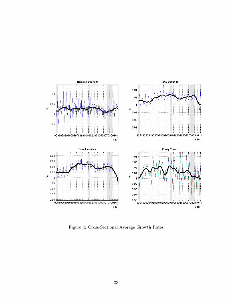
Figure 4: Cross-Sectional Average Growth Rates

33

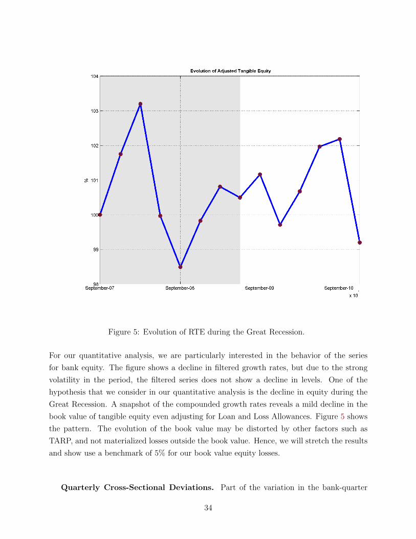
Figure 5: Evolution of RTE during the Great Recession.

For our quantitative analysis, we are particularly interested in the behavior of the series

for bank equity. The figure shows a decline in filtered growth rates, but due to the strong

volatility in the period, the filtered series does not show a decline in levels. One of the

hypothesis that we consider in our quantitative analysis is the decline in equity during the

Great Recession. A snapshot of the compounded growth rates reveals a mild decline in the

book value of tangible equity even adjusting for Loan and Loss Allowances. Figure 5 shows

the pattern. The evolution of the book value may be distorted by other factors such as

TARP, and not materialized losses outside the book value. Hence, we will stretch the results

and show use a benchmark of 5% for our book value equity losses.

Quarterly Cross-Sectional Deviations. Part of the variation in the bank-quarter

34

statistics presented above have a common component, including seasonality, nominal changes

in the time series and aggregate trends. To decompose the variation of these liabilities into

their common component, we present the summary statistics in terms of deviations of these

variables from their quarterly cross-sectional averages. Table 3 presents the results:

Variable Mean Std. Dev. Ndev TD 0 0.084 771369dev DD 0 0.183 777932dev TL 0 0.069 773629dev TE 0 0.081 769073dev RTE 0 0.096 766803dev E 0 0.071 774401dev RE 0 0.085 769329

Table 3: Summary statistics

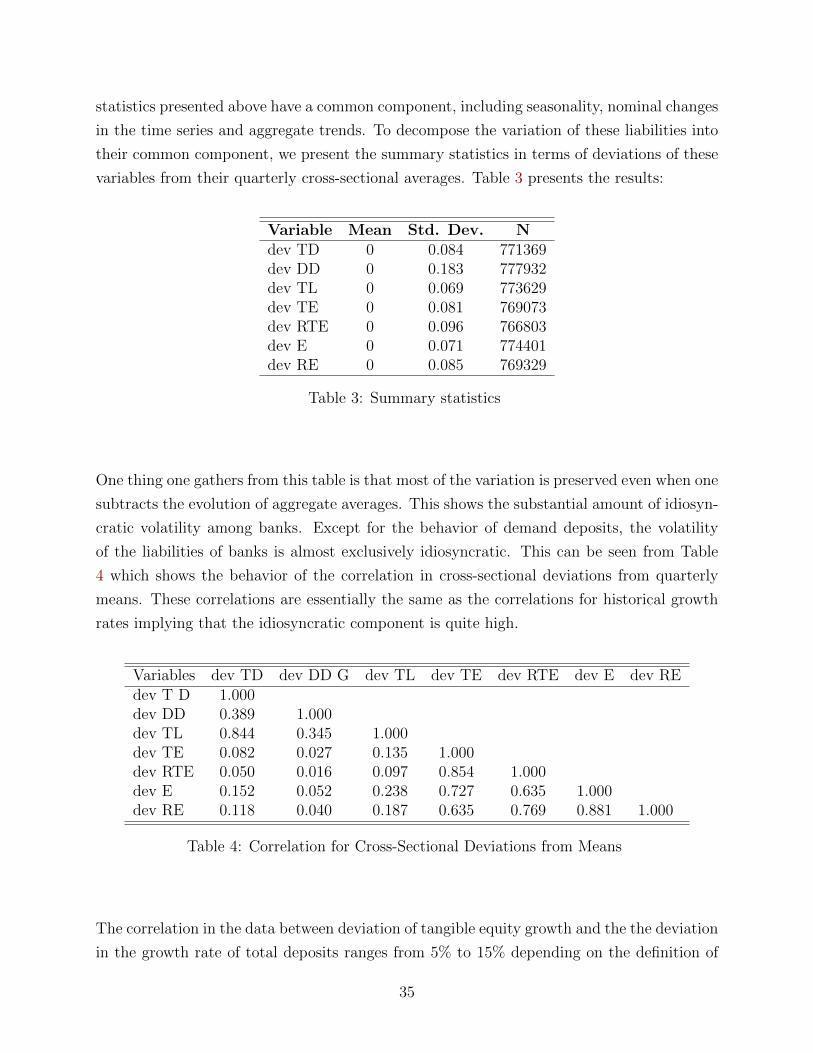
One thing one gathers from this table is that most of the variation is preserved even when one

subtracts the evolution of aggregate averages. This shows the substantial amount of idiosyn-

cratic volatility among banks. Except for the behavior of demand deposits, the volatility

of the liabilities of banks is almost exclusively idiosyncratic. This can be seen from Table

4 which shows the behavior of the correlation in cross-sectional deviations from quarterly

means. These correlations are essentially the same as the correlations for historical growth

rates implying that the idiosyncratic component is quite high.

Variables dev TD dev DD G dev TL dev TE dev RTE dev E dev REdev T D 1.000dev DD 0.389 1.000dev TL 0.844 0.345 1.000dev TE 0.082 0.027 0.135 1.000dev RTE 0.050 0.016 0.097 0.854 1.000dev E 0.152 0.052 0.238 0.727 0.635 1.000dev RE 0.118 0.040 0.187 0.635 0.769 0.881 1.000

Table 4: Correlation for Cross-Sectional Deviations from Means

The correlation in the data between deviation of tangible equity growth and the the deviation

in the growth rate of total deposits ranges from 5% to 15% depending on the definition of

35

−0.2 −0.1 0 0.1 0.2 0.30

5

10

15

20

25

30

35

40Deposits Growth (pre 2007 dev. from mean)

−0.2 −0.1 0 0.1 0.2 0.30

10

20

30

40

50

60Tan Equity Growth (pre 2007 dev. from mean)

−0.2 −0.1 0 0.1 0.2 0.30

5

10

15

20

25

30

35

40Deposits Growth (post 2007 dev. from mean)

−0.2 −0.1 0 0.1 0.2 0.30

10

20

30

40

50

60Tan Equity Growth (post 2007 dev. from mean)

Figure 6: Cross-Sectional Distribution of Deviation from Cross-Sectional Average GrowthRates

equity that we use. In the model, this correlation will be very high (though not 1) because

deposit volatility is the only source of risk for banks. In practice, banks face other important

sources of risks such as loan risk, duration risk and trading risk. This figure however implies

that deposit withdrawal risks are non-negligible risks for banks.

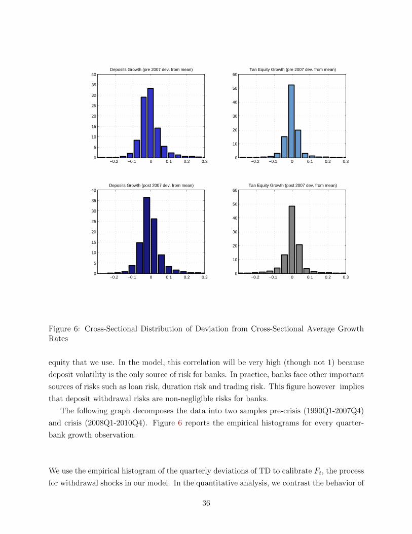
The following graph decomposes the data into two samples pre-crisis (1990Q1-2007Q4)

and crisis (2008Q1-2010Q4). Figure 6 reports the empirical histograms for every quarter-

bank growth observation.

We use the empirical histogram of the quarterly deviations of TD to calibrate Ft, the process

for withdrawal shocks in our model. In the quantitative analysis, we contrast the behavior of

36

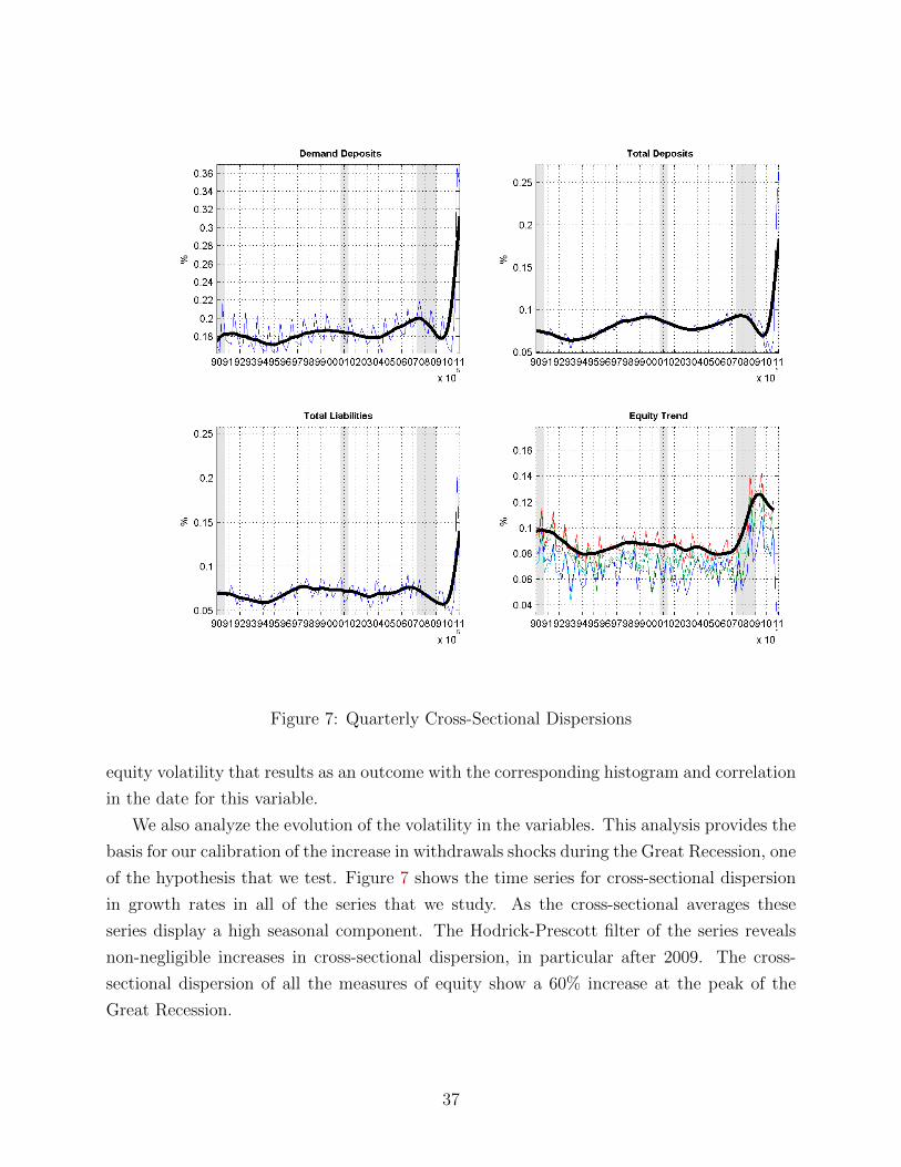
Figure 7: Quarterly Cross-Sectional Dispersions

equity volatility that results as an outcome with the corresponding histogram and correlation

in the date for this variable.

We also analyze the evolution of the volatility in the variables. This analysis provides the

basis for our calibration of the increase in withdrawals shocks during the Great Recession, one

of the hypothesis that we test. Figure 7 shows the time series for cross-sectional dispersion

in growth rates in all of the series that we study. As the cross-sectional averages these

series display a high seasonal component. The Hodrick-Prescott filter of the series reveals

non-negligible increases in cross-sectional dispersion, in particular after 2009. The cross-

sectional dispersion of all the measures of equity show a 60% increase at the peak of the

Great Recession.

37

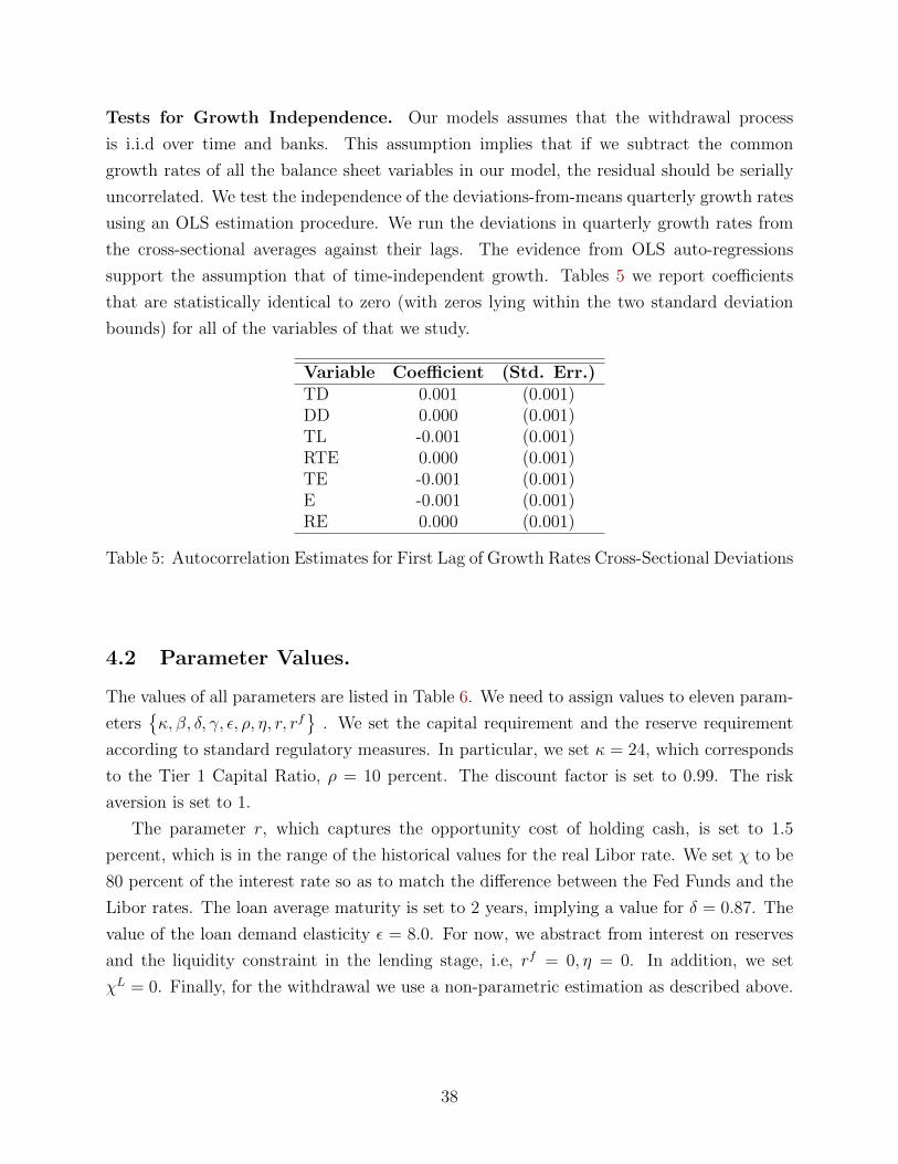
Tests for Growth Independence. Our models assumes that the withdrawal process

is i.i.d over time and banks. This assumption implies that if we subtract the common

growth rates of all the balance sheet variables in our model, the residual should be serially

uncorrelated. We test the independence of the deviations-from-means quarterly growth rates

using an OLS estimation procedure. We run the deviations in quarterly growth rates from

the cross-sectional averages against their lags. The evidence from OLS auto-regressions

support the assumption that of time-independent growth. Tables 5 we report coefficients

that are statistically identical to zero (with zeros lying within the two standard deviation

bounds) for all of the variables of that we study.

Variable Coefficient (Std. Err.)TD 0.001 (0.001)DD 0.000 (0.001)TL -0.001 (0.001)RTE 0.000 (0.001)TE -0.001 (0.001)E -0.001 (0.001)RE 0.000 (0.001)

Table 5: Autocorrelation Estimates for First Lag of Growth Rates Cross-Sectional Deviations

4.2 Parameter Values.

The values of all parameters are listed in Table 6. We need to assign values to eleven param-

etersκ, β, δ, γ, ε, ρ, η, r, rf

. We set the capital requirement and the reserve requirement

according to standard regulatory measures. In particular, we set κ = 24, which corresponds

to the Tier 1 Capital Ratio, ρ = 10 percent. The discount factor is set to 0.99. The risk

aversion is set to 1.

The parameter r, which captures the opportunity cost of holding cash, is set to 1.5

percent, which is in the range of the historical values for the real Libor rate. We set χ to be

80 percent of the interest rate so as to match the difference between the Fed Funds and the

Libor rates. The loan average maturity is set to 2 years, implying a value for δ = 0.87. The

value of the loan demand elasticity ε = 8.0. For now, we abstract from interest on reserves

and the liquidity constraint in the lending stage, i.e, rf = 0, η = 0. In addition, we set

χL = 0. Finally, for the withdrawal we use a non-parametric estimation as described above.

38

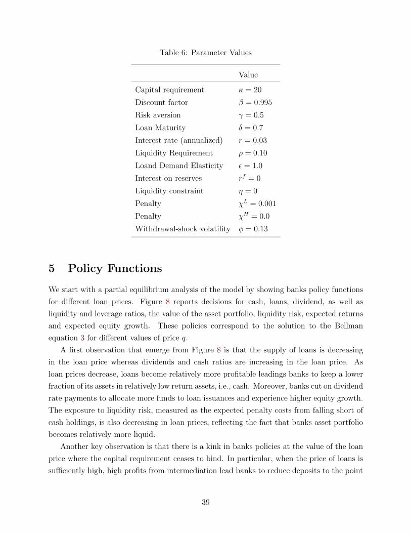
Table 6: Parameter Values

Value

Capital requirement κ = 20

Discount factor β = 0.995

Risk aversion γ = 0.5

Loan Maturity δ = 0.7

Interest rate (annualized) r = 0.03

Liquidity Requirement ρ = 0.10

Loand Demand Elasticity ε = 1.0

Interest on reserves rf = 0

Liquidity constraint η = 0

Penalty χL = 0.001

Penalty χH = 0.0

Withdrawal-shock volatility φ = 0.13

5 Policy Functions

We start with a partial equilibrium analysis of the model by showing banks policy functions

for different loan prices. Figure 8 reports decisions for cash, loans, dividend, as well as

liquidity and leverage ratios, the value of the asset portfolio, liquidity risk, expected returns

and expected equity growth. These policies correspond to the solution to the Bellman

equation 3 for different values of price q.

A first observation that emerge from Figure 8 is that the supply of loans is decreasing

in the loan price whereas dividends and cash ratios are increasing in the loan price. As

loan prices decrease, loans become relatively more profitable leadings banks to keep a lower

fraction of its assets in relatively low return assets, i.e., cash. Moreover, banks cut on dividend

rate payments to allocate more funds to loan issuances and experience higher equity growth.

The exposure to liquidity risk, measured as the expected penalty costs from falling short of

cash holdings, is also decreasing in loan prices, reflecting the fact that banks asset portfolio

becomes relatively more liquid.

Another key observation is that there is a kink in banks policies at the value of the loan

price where the capital requirement ceases to bind. In particular, when the price of loans is

sufficiently high, high profits from intermediation lead banks to reduce deposits to the point

39

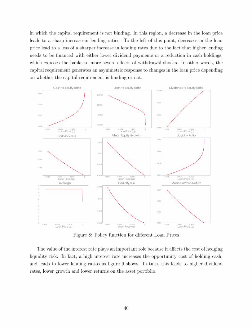
in which the capital requirement is not binding. In this region, a decrease in the loan price

leads to a sharp increase in lending ratios. To the left of this point, decreases in the loan

price lead to a less of a sharper increase in lending rates due to the fact that higher lending

needs to be financed with either lower dividend payments or a reduction in cash holdings,

which exposes the banks to more severe effects of withdrawal shocks. In other words, the

capital requirement generates an asymmetric response to changes in the loan price depending

on whether the capital requirement is binding or not.

0.9938 0.9959 0.9979 1

3.6242

4.5012

5.3782

6.2552

Cash-to-Equity Ratio

Loan Price (q)0.9938 0.9959 0.9979 1

15.0858

18.806

22.5261

26.2463

Loan-to-Equity Ratio

Loan Price (q)0.9938 0.9959 0.9979 1

0.0003

0.0068

0.0134

0.0199

Dividends-to-Equity Ratio

Loan Price (q)

0.9938 0.9959 0.9979 11

1.0033

1.0066

1.0099

Porfolio Value

Loan Price (q)0.9938 0.9959 0.9979 1

0.9801

0.9933

1.0065

1.0197

Mean Equity Growth

Loan Price (q)0.9938 0.9959 0.9979 1

0.1213

0.1786

0.2358

0.2931

Liquidity Ratio

Loan Price (q)

0.9938 0.9959 0.9979 115

16

17

18

19

20

21

22

23

24

25

26Leverage

Loan Price (q)0.9938 0.9959 0.9979 1

0.0002

0.3861

0.772

1.1579

Liquidity Risk

Loan Price (q)0.9938 0.9959 0.9979 1

0.9801

0.9933

1.0065

1.0197

Mean Portfolio Return

Loan Price (q)

Figure 8: Policy function for different Loan Prices

The value of the interest rate plays an important role because it affects the cost of hedging

liquidity risk. In fact, a high interest rate increases the opportunity cost of holding cash,

and leads to lower lending ratios as figure 9 shows. In turn, this leads to higher dividend

rates, lower growth and lower returns on the asset portfolio.

40

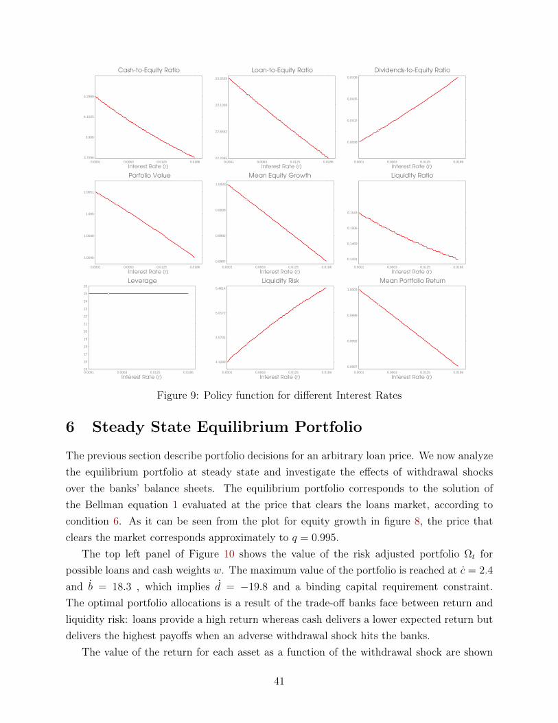
0.0001 0.0063 0.0125 0.01863.7096

3.906

4.1025

4.2989

Cash-to-Equity Ratio

Interest Rate (r)0.0001 0.0063 0.0125 0.0186

22.2065

22.6552

23.1038

23.5525

Loan-to-Equity Ratio

Interest Rate (r)0.0001 0.0063 0.0125 0.0186

0.0098

0.0102

0.0105

0.0108

Dividends-to-Equity Ratio

Interest Rate (r)

0.0001 0.0063 0.0125 0.0186

1.0046

1.0048

1.005

1.0051

Porfolio Value

Interest Rate (r)0.0001 0.0063 0.0125 0.0186

0.9987

0.9992

0.9998

1.0003

Mean Equity Growth

Interest Rate (r)0.0001 0.0063 0.0125 0.0186

0.1431

0.1469

0.1506

0.1543

Liquidity Ratio

Interest Rate (r)

0.0001 0.0063 0.0125 0.018615

16

17

18

19

20

21

22

23

24

25

26Leverage

Interest Rate (r)0.0001 0.0063 0.0125 0.0186

4.1289

4.5731

5.0172

5.4614

Liquidity Risk

Interest Rate (r)0.0001 0.0063 0.0125 0.0186

0.9987

0.9992

0.9998

1.0003

Mean Portfolio Return

Interest Rate (r)

Figure 9: Policy function for different Interest Rates

6 Steady State Equilibrium Portfolio

The previous section describe portfolio decisions for an arbitrary loan price. We now analyze

the equilibrium portfolio at steady state and investigate the effects of withdrawal shocks

over the banks’ balance sheets. The equilibrium portfolio corresponds to the solution of

the Bellman equation 1 evaluated at the price that clears the loans market, according to

condition 6. As it can be seen from the plot for equity growth in figure 8, the price that

clears the market corresponds approximately to q = 0.995.

The top left panel of Figure 10 shows the value of the risk adjusted portfolio Ωt for

possible loans and cash weights w. The maximum value of the portfolio is reached at c = 2.4

and b = 18.3 , which implies d = −19.8 and a binding capital requirement constraint.

The optimal portfolio allocations is a result of the trade-off banks face between return and

liquidity risk: loans provide a high return whereas cash delivers a lower expected return but

delivers the highest payoffs when an adverse withdrawal shock hits the banks.

The value of the return for each asset as a function of the withdrawal shock are shown

41

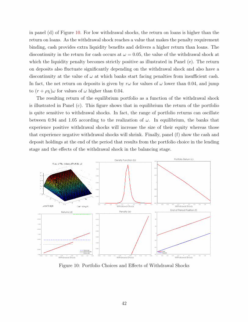
in panel (d) of Figure 10. For low withdrawal shocks, the return on loans is higher than the

return on loans. As the withdrawal shock reaches a value that makes the penalty requirement

binding, cash provides extra liquidity benefits and delivers a higher return than loans. The

discontinuity in the return for cash occurs at ω = 0.05, the value of the withdrawal shock at

which the liquidity penalty becomes strictly positive as illustrated in Panel (e). The return

on deposits also fluctuate significantly depending on the withdrawal shock and also have a

discontinuity at the value of ω at which banks start facing penalties from insufficient cash.

In fact, the net return on deposits is given by rω for values of ω lower than 0.04, and jump

to (r + ρχ)ω for values of ω higher than 0.04.

The resulting return of the equilibrium portfolio as a function of the withdrawal shock

is illustrated in Panel (c). This figure shows that in equilibrium the return of the portfolio

is quite sensitive to withdrawal shocks. In fact, the range of portfolio returns can oscillate

between 0.94 and 1.05 according to the realization of ω. In equilibrium, the banks that

experience positive withdrawal shocks will increase the size of their equity whereas those

that experience negative withdrawal shocks will shrink. Finally, panel (f) show the cash and

deposit holdings at the end of the period that results from the portfolio choice in the lending

stage and the effects of the withdrawal shock in the balancing stage.

−0.5 −0.4 −0.3 −0.2 −0.1 0 0.1 0.2 0.3 0.40

0.002

0.004

0.006

0.008

0.01

0.012

Withdrawal Shock

Density Function (b)

−1 −0.8 −0.6 −0.4 −0.2 0 0.2 0.4 0.6 0.8 10.94

0.96

0.98

1

1.02

1.04

1.06

Withdrawal Shock

Portfolio Return (c)

−0.25 −0.2 −0.15 −0.1 −0.05 0 0.05 0.1 0.15 0.2 0.250.999

0.9995

1

1.0005

1.001

1.0015

1.002

1.0025

1.003

Withdrawal Shock

Returns (d)

Return loanReturn depositsReturn cash

−0.25 −0.2 −0.15 −0.1 −0.05 0 0.05 0.1 0.15 0.2 0.250

0.002

0.004

0.006

0.008

0.01

0.012

0.014

Withdrawal Shock

Penalty (e)

−1 −0.8 −0.6 −0.4 −0.2 0 0.2 0.4 0.6 0.8 1−60

−40

−20

0

20

40

60

Withdrawal Shock

End of Period Position (f)

CashDeposits

Figure 10: Portfolio Choices and Effects of Withdrawal Shocks

42

7 Transitional Dynamics

This section studies how the economy responds to different shocks. For this purpose, we

consider an economy that is at steady state at period t = 0 and experience an unanticipated

permanent shock. The shocks we consider are equity losses, credit demand shocks, a tighten-

ing of capital requirements, uncertainty shocks and rise in funding costs. For each shock, we

analyze the transitional dynamics of banking and monetary indicators. The panels 11-15 in

this section show the aggregate dynamics. Each panel shows that path of total lending, total

cash, loan prices, the return on loans, total equity and new loan issuances. In addition, we

also refer to the panels 23 -28 in the Appendix illustrate the dynamics of the individual banks

policies. The superior panel for each figure shows the cash-to-equity ratio, loan-to-equity

ratio and dividends-to-equity ratio. The intermediate panel shows the portfolio value, the

mean equity growth and the liquidity ratio. Finally, the inferior panel shows the liquidity

risk, bank value expressed in consumption units and the mean portfolio return.

7.1 Equity Losses

The first shock we consider is a sudden unexpected decline in bank equity, which can be

interpreted as capturing an unexpected rise in non-performing loans or losses from other

portions of the balance sheets. Figure 11 illustrates the response of the economy to equity

losses of 5 percent. A key result is that the economy experiences an immediate drop in loan

prices and converges back to the initial steady state. Hence, there is an amplification effect

on the value of the bank through the decline in the value of asset holdings.

Let us analyze the transitional dynamics in more detail. What explains the immediate

drop in loan prices? Suppose loan prices did not change at all. In this case, banks would

keep the same lending ratios and total lending, computed as E1b1 −E0b0(1− δ), would fall.

If loan prices do not change, however, the demand for loans would remain unchanged leading

to an excess demand for loans. In equilibrium, this means that loan prices need to drop on

impact. Low loan prices also mean that banks have high return from lending, and equity

growth, as we analyzed in section 5. Hence, as the economy converges to the steady state,

the increase in equity leads to a monotonic increase in loan prices.

The behavior of dividend rates reflect a trade-off in the model. On the one hand, equity

losses lead to a rise in the return on loans that makes cutting dividend payments more

attractive. On the other hand, general equilibrium effects generate wealth effects generating

an increase in dividend rates. Overall, we find that that the first effect prevails.

The volume of bank lending follows a persistent decline. As the price of loans drop on

impact, there is a sharp decline in the demand for new issuances, which is larger than the

43

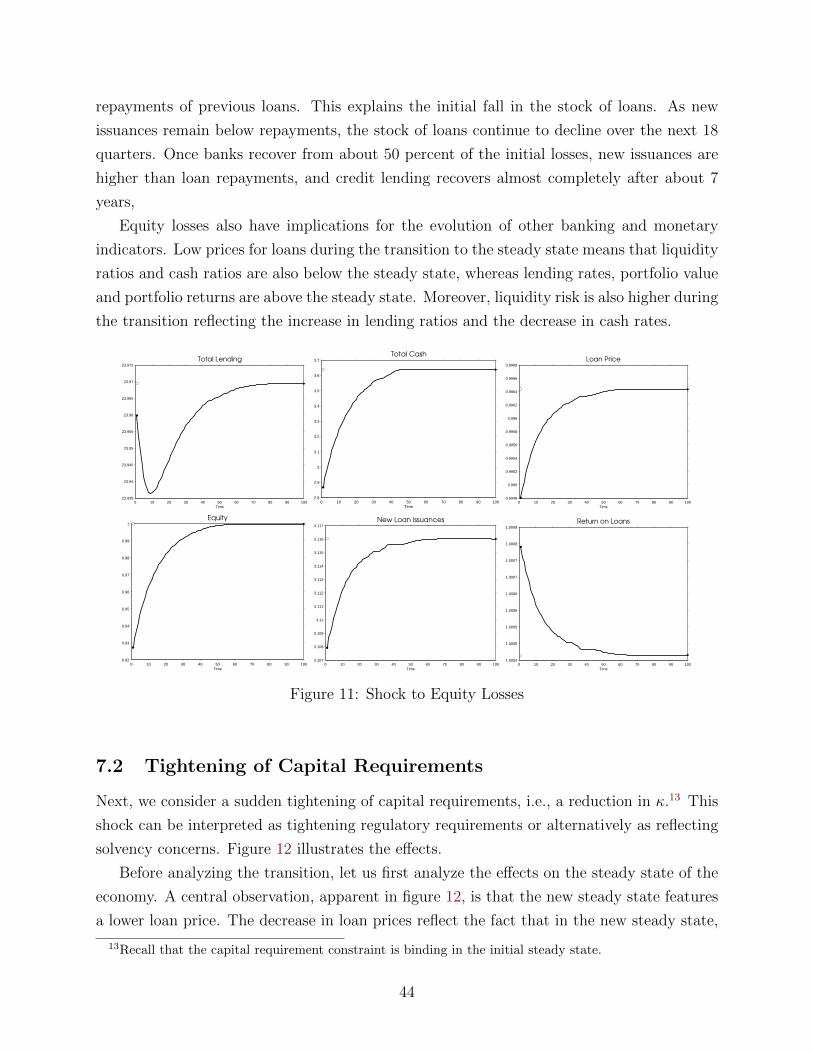
repayments of previous loans. This explains the initial fall in the stock of loans. As new

issuances remain below repayments, the stock of loans continue to decline over the next 18

quarters. Once banks recover from about 50 percent of the initial losses, new issuances are

higher than loan repayments, and credit lending recovers almost completely after about 7

years,

Equity losses also have implications for the evolution of other banking and monetary

indicators. Low prices for loans during the transition to the steady state means that liquidity

ratios and cash ratios are also below the steady state, whereas lending rates, portfolio value

and portfolio returns are above the steady state. Moreover, liquidity risk is also higher during

the transition reflecting the increase in lending ratios and the decrease in cash rates.

0 10 20 30 40 50 60 70 80 90 10023.935

23.94

23.945

23.95

23.955

23.96

23.965

23.97

23.975

Time

Total Lending

0 10 20 30 40 50 60 70 80 90 1002.8

2.9

3

3.1

3.2

3.3

3.4

3.5

3.6

3.7

Time

Total Cash

0 10 20 30 40 50 60 70 80 90 1000.9948

0.995

0.9952

0.9954

0.9956

0.9958

0.996

0.9962

0.9964

0.9966

0.9968

Time

Loan Price

0 10 20 30 40 50 60 70 80 90 1000.92

0.93

0.94

0.95

0.96

0.97

0.98

0.99

1

Time

Equity

0 10 20 30 40 50 60 70 80 90 1003.107

3.108

3.109

3.11

3.111

3.112

3.113

3.114

3.115

3.116

3.117

Time

New Loan Issuances

0 10 20 30 40 50 60 70 80 90 1001.0004

1.0005

1.0005

1.0006

1.0006

1.0007

1.0007

1.0008

1.0008

Time

Return on Loans

Figure 11: Shock to Equity Losses

7.2 Tightening of Capital Requirements

Next, we consider a sudden tightening of capital requirements, i.e., a reduction in κ.13 This

shock can be interpreted as tightening regulatory requirements or alternatively as reflecting

solvency concerns. Figure 12 illustrates the effects.

Before analyzing the transition, let us first analyze the effects on the steady state of the

economy. A central observation, apparent in figure 12, is that the new steady state features

a lower loan price. The decrease in loan prices reflect the fact that in the new steady state,

13Recall that the capital requirement constraint is binding in the initial steady state.

44

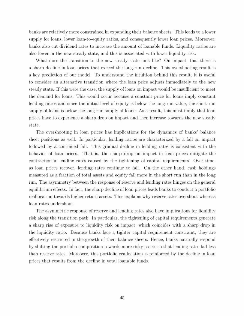
banks are relatively more constrained in expanding their balance sheets. This leads to a lower

supply for loans, lower loan-to-equity ratios, and consequently lower loan prices. Moreover,

banks also cut dividend rates to increase the amount of loanable funds. Liquidity ratios are

also lower in the new steady state, and this is associated with lower liquidity risk.

What does the transition to the new steady state look like? On impact, that there is

a sharp decline in loan prices that exceed the long-run decline. This overshooting result is

a key prediction of our model. To understand the intuition behind this result, it is useful

to consider an alternative transition where the loan price adjusts immediately to the new

steady state. If this were the case, the supply of loans on impact would be insufficient to meet

the demand for loans. This would occur because a constant price for loans imply constant

lending ratios and since the initial level of equity is below the long-run value, the short-run

supply of loans is below the long-run supply of loans. As a result, this must imply that loan

prices have to experience a sharp drop on impact and then increase towards the new steady

state.

The overshooting in loan prices has implications for the dynamics of banks’ balance

sheet positions as well. In particular, lending ratios are characterized by a fall on impact

followed by a continued fall. This gradual decline in lending rates is consistent with the

behavior of loan prices. That is, the sharp drop on impact in loan prices mitigate the

contraction in lending rates caused by the tightening of capital requirements. Over time,

as loan prices recover, lending rates continue to fall. On the other hand, cash holdings

measured as a fraction of total assets and equity fall more in the short run than in the long

run. The asymmetry between the response of reserve and lending rates hinges on the general

equilibrium effects. In fact, the sharp decline of loan prices leads banks to conduct a portfolio

reallocation towards higher return assets. This explains why reserve rates overshoot whereas

loan rates undershoot.

The asymmetric response of reserve and lending rates also have implications for liquidity

risk along the transition path. In particular, the tightening of capital requirements generate

a sharp rise of exposure to liquidity risk on impact, which coincides with a sharp drop in

the liquidity ratio. Because banks face a tighter capital requirement constraint, they are

effectively restricted in the growth of their balance sheets. Hence, banks naturally respond

by shifting the portfolio composition towards more risky assets so that lending rates fall less

than reserve rates. Moreover, this portfolio reallocation is reinforced by the decline in loan

prices that results from the decline in total loanable funds.

45

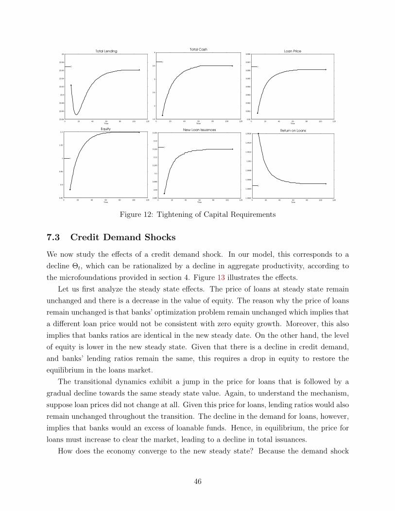
0 20 40 60 80 100 12023.84

23.86

23.88

23.9

23.92

23.94

23.96

23.98

24

Time

Total Lending

0 20 40 60 80 100 1201.5

2

2.5

3

3.5

4

Time

Total Cash

0 20 40 60 80 100 1200.99

0.991

0.992

0.993

0.994

0.995

0.996

0.997

0.998

Time

Loan Price

0 20 40 60 80 100 1200.85

0.9

0.95

1

1.05

1.1

Time

Equity

0 20 40 60 80 100 1203.085

3.09

3.095

3.1

3.105

3.11

3.115

3.12

3.125

Time

New Loan Issuances

0 20 40 60 80 100 1201.0002

1.0004

1.0006

1.0008

1.001

1.0012

1.0014

1.0016

Time

Return on Loans

Figure 12: Tightening of Capital Requirements

7.3 Credit Demand Shocks

We now study the effects of a credit demand shock. In our model, this corresponds to a

decline Θt, which can be rationalized by a decline in aggregate productivity, according to

the microfoundations provided in section 4. Figure 13 illustrates the effects.

Let us first analyze the steady state effects. The price of loans at steady state remain

unchanged and there is a decrease in the value of equity. The reason why the price of loans

remain unchanged is that banks’ optimization problem remain unchanged which implies that

a different loan price would not be consistent with zero equity growth. Moreover, this also

implies that banks ratios are identical in the new steady date. On the other hand, the level

of equity is lower in the new steady state. Given that there is a decline in credit demand,

and banks’ lending ratios remain the same, this requires a drop in equity to restore the

equilibrium in the loans market.

The transitional dynamics exhibit a jump in the price for loans that is followed by a

gradual decline towards the same steady state value. Again, to understand the mechanism,

suppose loan prices did not change at all. Given this price for loans, lending ratios would also

remain unchanged throughout the transition. The decline in the demand for loans, however,

implies that banks would an excess of loanable funds. Hence, in equilibrium, the price for

loans must increase to clear the market, leading to a decline in total issuances.

How does the economy converge to the new steady state? Because the demand shock

46

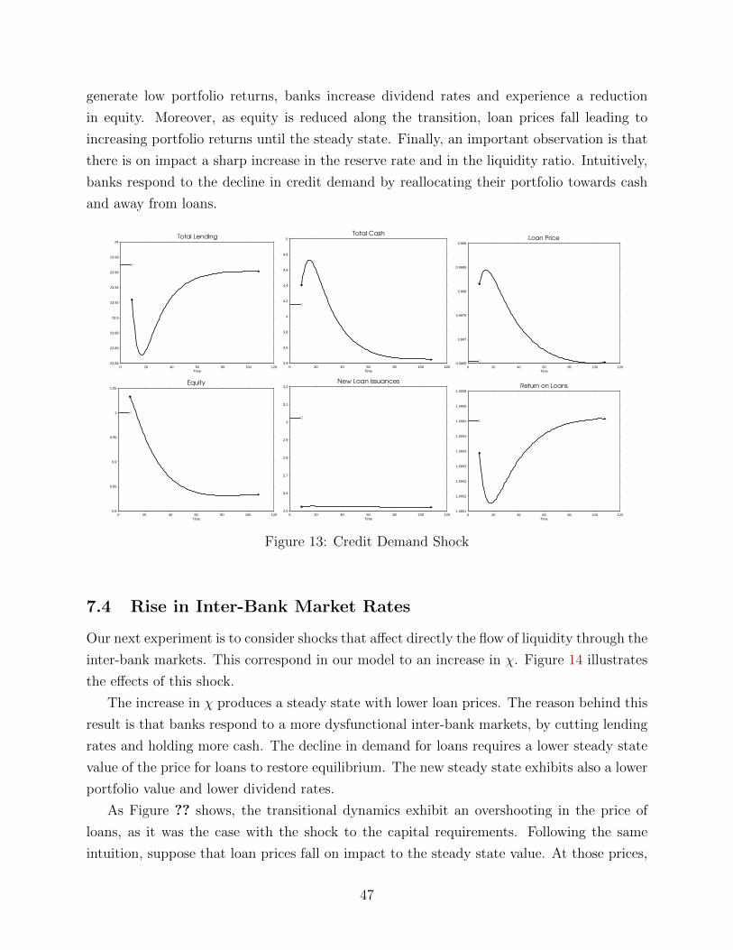
generate low portfolio returns, banks increase dividend rates and experience a reduction

in equity. Moreover, as equity is reduced along the transition, loan prices fall leading to

increasing portfolio returns until the steady state. Finally, an important observation is that

there is on impact a sharp increase in the reserve rate and in the liquidity ratio. Intuitively,

banks respond to the decline in credit demand by reallocating their portfolio towards cash

and away from loans.

0 20 40 60 80 100 12023.84

23.86

23.88

23.9

23.92

23.94

23.96

23.98

24

Time

Total Lending

0 20 40 60 80 100 1203.4

3.6

3.8

4

4.2

4.4

4.6

4.8

5

Time

Total Cash

0 20 40 60 80 100 1200.9965

0.997

0.9975

0.998

0.9985

0.999

Time

Loan Price

0 20 40 60 80 100 1200.8

0.85

0.9

0.95

1

1.05

Time

Equity

0 20 40 60 80 100 1202.5

2.6

2.7

2.8

2.9

3

3.1

3.2

Time

New Loan Issuances

0 20 40 60 80 100 1201.0001

1.0002

1.0002

1.0003

1.0003

1.0004

1.0004

1.0005

1.0005

Time

Return on Loans

Figure 13: Credit Demand Shock

7.4 Rise in Inter-Bank Market Rates

Our next experiment is to consider shocks that affect directly the flow of liquidity through the

inter-bank markets. This correspond in our model to an increase in χ. Figure 14 illustrates

the effects of this shock.

The increase in χ produces a steady state with lower loan prices. The reason behind this

result is that banks respond to a more dysfunctional inter-bank markets, by cutting lending

rates and holding more cash. The decline in demand for loans requires a lower steady state

value of the price for loans to restore equilibrium. The new steady state exhibits also a lower

portfolio value and lower dividend rates.

As Figure ?? shows, the transitional dynamics exhibit an overshooting in the price of

loans, as it was the case with the shock to the capital requirements. Following the same

intuition, suppose that loan prices fall on impact to the steady state value. At those prices,

47

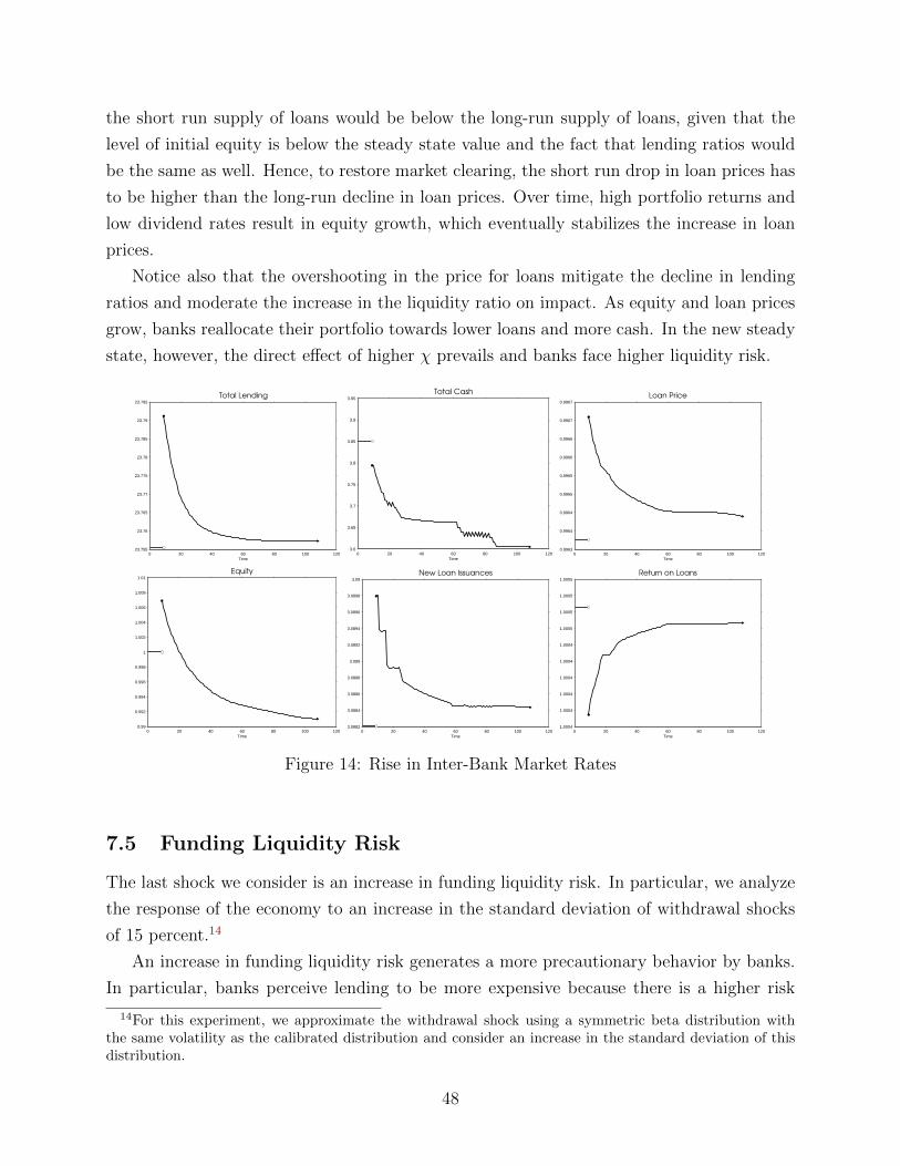
the short run supply of loans would be below the long-run supply of loans, given that the

level of initial equity is below the steady state value and the fact that lending ratios would

be the same as well. Hence, to restore market clearing, the short run drop in loan prices has

to be higher than the long-run decline in loan prices. Over time, high portfolio returns and

low dividend rates result in equity growth, which eventually stabilizes the increase in loan

prices.

Notice also that the overshooting in the price for loans mitigate the decline in lending

ratios and moderate the increase in the liquidity ratio on impact. As equity and loan prices

grow, banks reallocate their portfolio towards lower loans and more cash. In the new steady

state, however, the direct effect of higher χ prevails and banks face higher liquidity risk.

0 20 40 60 80 100 12023.755

23.76

23.765

23.77

23.775

23.78

23.785

23.79

23.795

Time

Total Lending

0 20 40 60 80 100 1203.6

3.65

3.7

3.75

3.8

3.85

3.9

3.95

Time

Total Cash

0 20 40 60 80 100 1200.9963

0.9964

0.9964

0.9965

0.9965

0.9966

0.9966

0.9967

0.9967

Time

Loan Price

0 20 40 60 80 100 1200.99

0.992

0.994

0.996

0.998

1

1.002

1.004

1.006

1.008

1.01

Time

Equity

0 20 40 60 80 100 1203.0882

3.0884

3.0886

3.0888

3.089

3.0892

3.0894

3.0896

3.0898

3.09

Time

New Loan Issuances

0 20 40 60 80 100 1201.0004

1.0004

1.0004

1.0004

1.0004

1.0004

1.0005

1.0005

1.0005

1.0005

Time

Return on Loans

Figure 14: Rise in Inter-Bank Market Rates

7.5 Funding Liquidity Risk

The last shock we consider is an increase in funding liquidity risk. In particular, we analyze

the response of the economy to an increase in the standard deviation of withdrawal shocks

of 15 percent.14

An increase in funding liquidity risk generates a more precautionary behavior by banks.

In particular, banks perceive lending to be more expensive because there is a higher risk

14For this experiment, we approximate the withdrawal shock using a symmetric beta distribution withthe same volatility as the calibrated distribution and consider an increase in the standard deviation of thisdistribution.

48

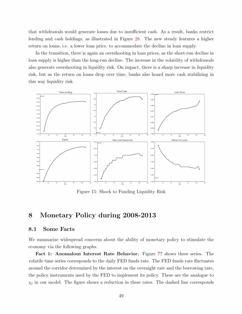
that withdrawals would generate losses due to insufficient cash. As a result, banks restrict

lending and cash holdings, as illustrated in Figure 28. The new steady features a higher

return on loans, i.e. a lower loan price, to accommodate the decline in loan supply.

In the transition, there is again an overshooting in loan prices, as the short-run decline in

loan supply is higher than the long-run decline. The increase in the volatility of withdrawals

also generate overshooting in liquidity risk. On impact, there is a sharp increase in liquidity

risk, but as the return on loans drop over time, banks also hoard more cash stabilizing in

this way liquidity risk.

0 20 40 60 80 100 12021.23

21.232

21.234

21.236

21.238

21.24

21.242

21.244

21.246

21.248

21.25

Time

Total Lending

0 20 40 60 80 100 1206.15

6.2

6.25

6.3

6.35

6.4

6.45

6.5

Time

Total Cash

0 20 40 60 80 100 1200.9955

0.9956

0.9956

0.9957

0.9957

0.9958

0.9958

0.9959

Time

Loan Price

0 20 40 60 80 100 1200.994

0.996

0.998

1

1.002

1.004

1.006

1.008

1.01

1.012

1.014

Time

Equity

0 20 40 60 80 100 1202.7612

2.7614

2.7616

2.7618

2.762

2.7622

2.7624

Time

New Loan Issuances

0 20 40 60 80 100 1201.0005

1.0005

1.0005

1.0006

1.0006

1.0006

1.0006

Time

Return on Loans

Figure 15: Shock to Funding Liquidity Risk

8 Monetary Policy during 2008-2013

8.1 Some Facts

We summarize widespread concerns about the ability of monetary policy to stimulate the

economy via the following graphs.

Fact 1: Anomalous Interest Rate Behavior. Figure ?? shows three series. The

volatile time series corresponds to the daily FED funds rate. The FED funds rate fluctuates

around the corridor determined by the interest on the overnight rate and the borrowing rate,

the policy instruments used by the FED to implement its policy. These are the analogue to

χt in our model. The figure shows a reduction in these rates. The dashed line corresponds

49

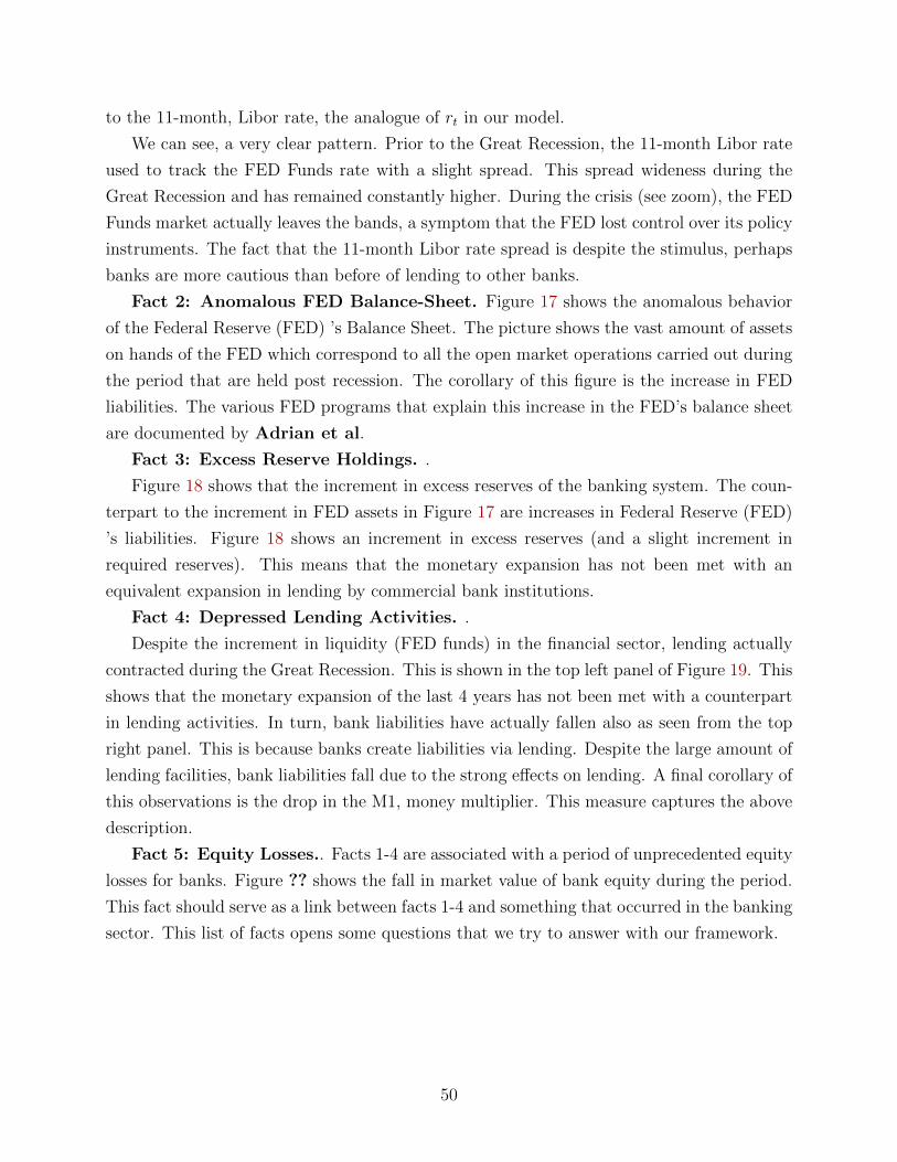
to the 11-month, Libor rate, the analogue of rt in our model.

We can see, a very clear pattern. Prior to the Great Recession, the 11-month Libor rate

used to track the FED Funds rate with a slight spread. This spread wideness during the

Great Recession and has remained constantly higher. During the crisis (see zoom), the FED

Funds market actually leaves the bands, a symptom that the FED lost control over its policy

instruments. The fact that the 11-month Libor rate spread is despite the stimulus, perhaps

banks are more cautious than before of lending to other banks.

Fact 2: Anomalous FED Balance-Sheet. Figure 17 shows the anomalous behavior

of the Federal Reserve (FED) ’s Balance Sheet. The picture shows the vast amount of assets

on hands of the FED which correspond to all the open market operations carried out during

the period that are held post recession. The corollary of this figure is the increase in FED

liabilities. The various FED programs that explain this increase in the FED’s balance sheet

are documented by Adrian et al.

Fact 3: Excess Reserve Holdings. .

Figure 18 shows that the increment in excess reserves of the banking system. The coun-

terpart to the increment in FED assets in Figure 17 are increases in Federal Reserve (FED)

’s liabilities. Figure 18 shows an increment in excess reserves (and a slight increment in

required reserves). This means that the monetary expansion has not been met with an

equivalent expansion in lending by commercial bank institutions.

Fact 4: Depressed Lending Activities. .

Despite the increment in liquidity (FED funds) in the financial sector, lending actually

contracted during the Great Recession. This is shown in the top left panel of Figure 19. This

shows that the monetary expansion of the last 4 years has not been met with a counterpart

in lending activities. In turn, bank liabilities have actually fallen also as seen from the top

right panel. This is because banks create liabilities via lending. Despite the large amount of

lending facilities, bank liabilities fall due to the strong effects on lending. A final corollary of

this observations is the drop in the M1, money multiplier. This measure captures the above

description.

Fact 5: Equity Losses.. Facts 1-4 are associated with a period of unprecedented equity

losses for banks. Figure ?? shows the fall in market value of bank equity during the period.

This fact should serve as a link between facts 1-4 and something that occurred in the banking

sector. This list of facts opens some questions that we try to answer with our framework.

50

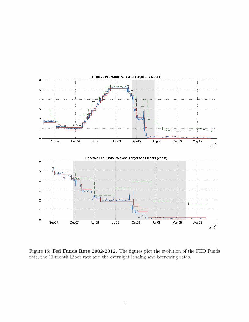
Figure 16: Fed Funds Rate 2002-2012. The figures plot the evolution of the FED Fundsrate, the 11-month Libor rate and the overnight lending and borrowing rates.

51

Figure 17: Federal Reserve Assets: 2002-2012. The figure shows the expansion in theFED’s asset holdings. The magnitudes are in Millions of US$.

52

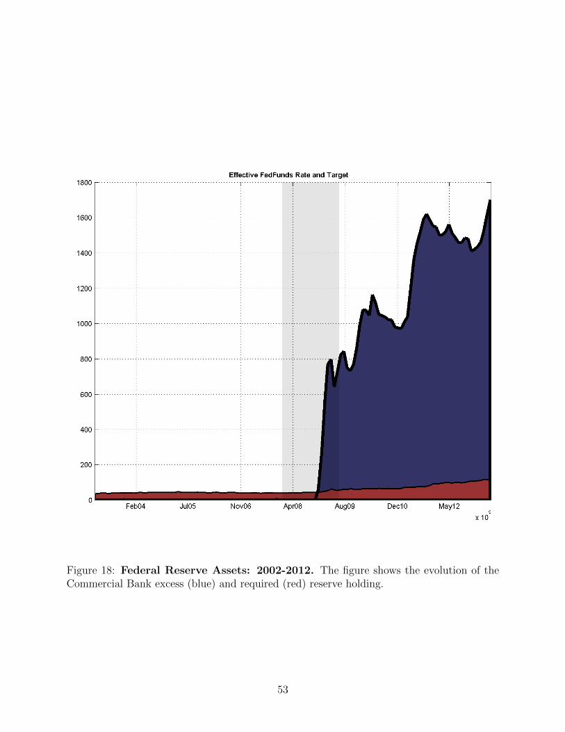
Figure 18: Federal Reserve Assets: 2002-2012. The figure shows the evolution of theCommercial Bank excess (blue) and required (red) reserve holding.

53

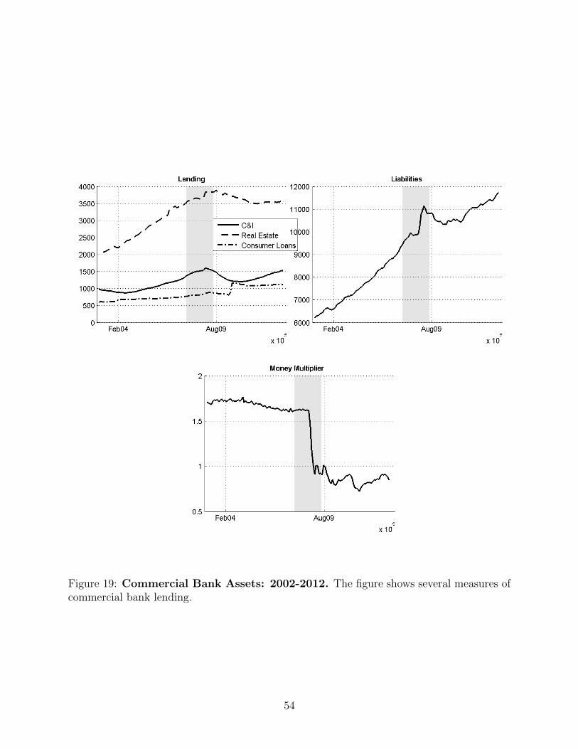
Figure 19: Commercial Bank Assets: 2002-2012. The figure shows several measures ofcommercial bank lending.

54

8.2 Some Questions

We use the model as a laboratory to answer whether monetary policy has been interrupted

after the Great Recession. The model’s answers will be based on the assumptions that we

make for the real sector. In other words, they are conditional on having monetary policy

working only through the lending channel. To answer these questions, we will again place the

model within its perfect foresight environment. We assume all policy the path for interest

rates is well defined.

This first questions concerns the equity losses experienced by banks. Bank equity losses

will work by a risk aversion effect. Upon suffering unexpected losses, banks will reduce the

amount of new lending relative to their equity. Thus it is natural to ask, can bank equity

losses, of the magnitude of the Great Recession can render monetary policy inoperative?

An immediate policy response was to implement a sequence of new bank regulations

via the Basel-III agreements. Basel-III tightens κ and η in our model. Hence, a direct

policy implication is the tightening of bank leverage and the improvement of bank ratios.

An indirect effect occurs via affecting bank incentives to pay dividends. Lower leverage will

decrease bank returns and hence, induce a smaller banking sector. Can bank tighter bank

regulation interrupt the lending channel?

During the Great Recession we saw that the FED funds rate was out of control for a

small period. Moreover, the 11-month Libor spread is above its average historical level. Can

greater withdrawal volatility explain this fact?

The fourth question is, can a reduction in loan demand explain the post recession pat-

terns?

8.3 Model Answers: A Narrative of the last 5 Years

Building on the analysis from the previous section, we now explore if there are plausible

shocks within our model that can lead to a severe contraction in the financial system similar

to the one experienced recently in the US economy. In particular, we construct a coun-

terfactual experiment where we hit the economy with various shocks, one at a time, in a

cumulative fashion. The first part of the experiment consists of 3 shocks. First, we consider

a shock to equity losses equivalent to 0.2 percent of total assets. The magnitude of this shock

corresponds to the unexpected losses of AAA-rated subprime MBS tranches, estimated by

Park (2011). Second, we consider a tightening of capital requirements along the new pre-

scriptions of Basel III, by which Tier 1 Capital ratio increases from 4 percent to 6 percent

over the course of 6 years. Third, we consider the introduction of a probability of a bank-run,

which we take for now be 3 percent. Specifically, what we do is introduce a small probability

55

event of banks losing the entire stock of deposits. This shock lasts for 1 year.15 Finally, we

consider a temporary demand shock to match an initial drop in loan issuances of 25 percent,

in line with Ivashina and Scharfstein (2010). This shock is assumed to last for 6 years in

order to capture the duration of the Great Recession.

Figure ?? shows the results of the counterfactual experiment. The thick broken line

represent the economy which is hit only by equity losses. The straight line represents the

economy hit by equity losses and by tighter capital requirements. Finally, the dashed line

represents the economy hit by the these two shocks plus the increase in withdrawal risk.

Notice that the first shock has only temporary effects while the second and third have

permanent effects since the change in capital requirements is permanent.

The results suggest that a combination of shocks is essential to account for the dynamics

of the US financial crisis. The drop in equity by itself is not enough to produce a large drop

in new loan issuances. Moreover, the drop in equity results in a counterfactual decrease in

cash holdings. Similarly, the tightening of capital requirements, contribute to a deepening

of the drop in credit, but also leads banks to hold less cash, not more. On the other hand,

the increase in withdrawal risk has the potential to increase cash holdings, unlike the shocks

to equity losses and the tightening of capital requirements. As can be seen from Figure ??,

the increase in withdrawal risk generates significant increase in liquidity risk, but general

equilibrium effects mitigate the effects over total reserves.

At this point, these shocks do not seem to be able to explain quantitatively the increase

in liquidity holdings by banks or the decline in lending. Our preliminary investigations,

however, suggest that large credit demand shocks are consistent with the increase in reserves

and the decline in lending observed in the data. Interestingly, demand shocks also lead to

increase in equity payouts, which suggest that credit demand shocks alone cannot explain

the key features of the financial crisis.

15To keep the mean fixed, we also introduce the possibility of a large increase in deposits with the sameprobability.

56

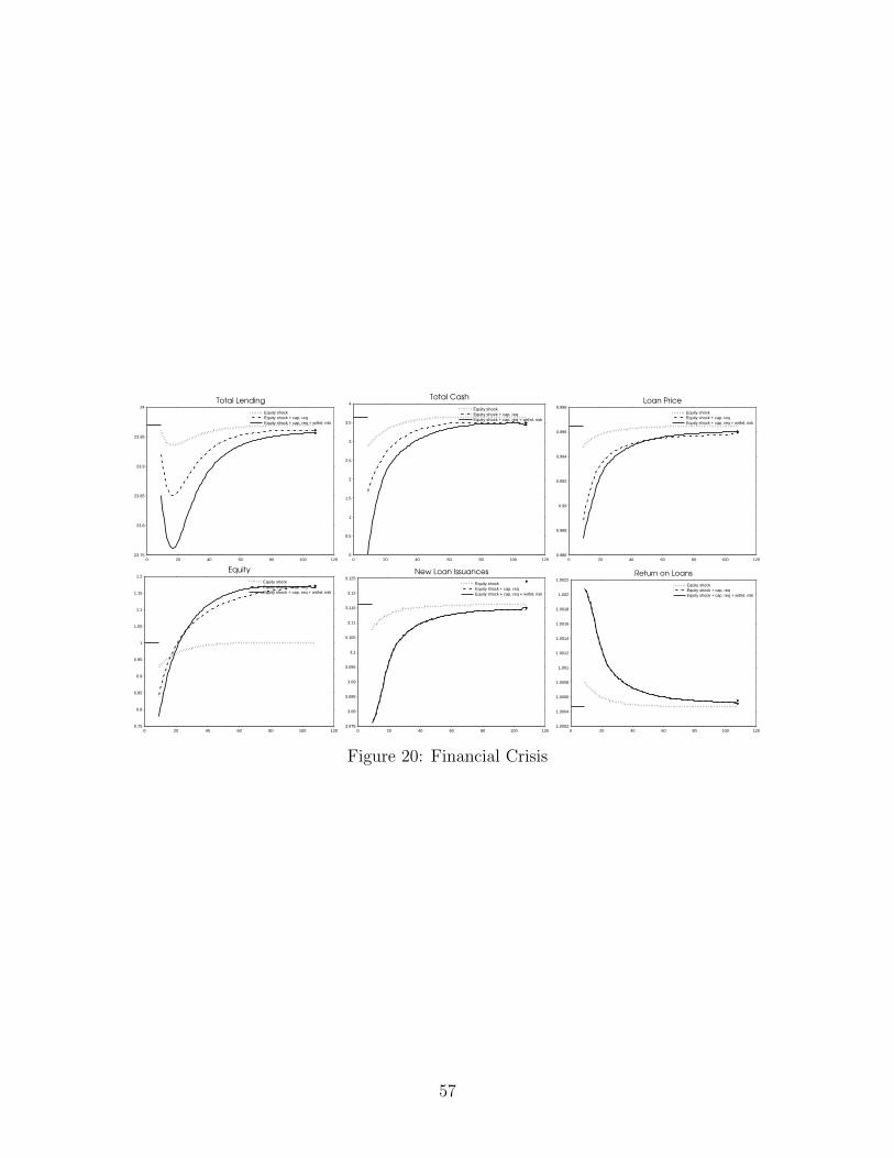
0 20 40 60 80 100 12023.75

23.8

23.85

23.9

23.95

24Total Lending

Equity shockEquity shock + cap. reqEquity shock + cap. req + withd. risk

0 20 40 60 80 100 1200

0.5

1

1.5

2

2.5

3

3.5

4Total Cash

Equity shockEquity shock + cap. reqEquity shock + cap. req + withd. risk

0 20 40 60 80 100 1200.986

0.988

0.99

0.992

0.994

0.996

0.998Loan Price

Equity shockEquity shock + cap. reqEquity shock + cap. req + withd. risk

0 20 40 60 80 100 1200.75

0.8

0.85

0.9

0.95

1

1.05

1.1

1.15

1.2Equity

Equity shockEquity shock + cap. reqEquity shock + cap. req + withd. risk

0 20 40 60 80 100 1203.075

3.08

3.085

3.09

3.095

3.1

3.105

3.11

3.115

3.12

3.125New Loan Issuances

Equity shockEquity shock + cap. reqEquity shock + cap. req + withd. risk

0 20 40 60 80 100 1201.0002

1.0004

1.0006

1.0008

1.001

1.0012

1.0014

1.0016

1.0018

1.002

1.0022Return on Loans

Equity shockEquity shock + cap. reqEquity shock + cap. req + withd. risk

Figure 20: Financial Crisis

57

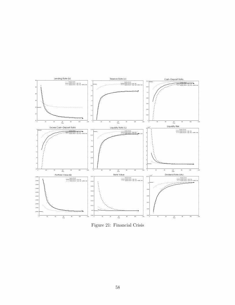
0 20 40 60 80 100 12020

22

24

26

28

30

32

Time

Lending Rate (b)

Equity shockEquity shock + cap. reqEquity shock + cap. req + withd. risk

0 20 40 60 80 100 1200

0.5

1

1.5

2

2.5

3

3.5

4

Time

Reserve Rate (c)

Equity shockEquity shock + cap. reqEquity shock + cap. req + withd. risk

0 20 40 60 80 100 1200

0.02

0.04

0.06

0.08

0.1

0.12

0.14

Time

Cash−Deposit Ratio

Equity shockEquity shock + cap. reqEquity shock + cap. req + withd. risk

0 20 40 60 80 100 120−10

−8

−6

−4

−2

0

2

4

Time

Excess Cash−Deposit Ratio

Equity shockEquity shock + cap. reqEquity shock + cap. req + withd. risk

0 20 40 60 80 100 1200

0.02

0.04

0.06

0.08

0.1

0.12

0.14

Time

Liquidity Ratio (L)

Equity shockEquity shock + cap. reqEquity shock + cap. req + withd. risk

0 20 40 60 80 100 1200

1

2

3

4

5

6

7

8

9x 10

−3

Time

Liquidity Risk

Equity shockEquity shock + cap. reqEquity shock + cap. req + withd. risk

0 20 40 60 80 100 1201

1.0001

1.0001

1.0002

1.0002

1.0003

1.0003

1.0004

1.0004

1.0005

1.0005

Time

Portfolio Value (Ω)

Equity shockEquity shock + cap. reqEquity shock + cap. req + withd. risk

0 20 40 60 80 100 1200.009

0.01

0.011

0.012

0.013

0.014

0.015

0.016

0.017

Time

Bank Value

Equity shockEquity shock + cap. reqEquity shock + cap. req + withd. risk

0 20 40 60 80 100 1209.95

9.96

9.97

9.98

9.99

10

10.01x 10

−3

Time

Dividend Rate (div)

Equity shockEquity shock + cap. reqEquity shock + cap. req + withd. risk

Figure 21: Financial Crisis

58

8.4 Effectiveness of Monetary Policy

INCOMPLETE

In this section, we study the effectiveness of monetary policy to stabilize financial markets.

In particular, we consider how a temporary reduction in χ can offset the impact of a series of

adverse shocks to financial markets studied above. The key question we address is whether

monetary policy is more or less effective in times of distress.

8.5 Potential Extensions

Before concluding, there are several extensions that we want to discuss. These extensions

will allow us a more thorough understanding of monetary transmission through this model.

Nominal contracts and other rigidities. We deliberately imposed assumptions in

our model so that lending contracts are real. Our model can be enriched to incorporate

features that may induce changes in prices, without corresponding movements in contracts.

The introduction of nominal debt contracts and price movements may help us understand

the role of Fisherian debt-deflation phenomena (see Krugman and Eggertson, for example.).

Another form of nominal contracts can be introduced onto the labor market. This form of

nominal friction, may help us evaluate the role of the interest rate channel.

Credit- Risk uncertainty. Although we have studied the effects of equity, these losses

are unforseen. We believe our model may have interesting effects if there are periods where

banks are aware, but uncertain, about potential equity losses.

A market for T-Bills. For tractability, we assumed that bank assets are either loans or

reserves. Thus, the model neglects a role for Treasury Bills which are a very important part

of bank balance sheets and are the main instrument for open market operations. Treasuries

are a special type of asset. Unlike other forms of bank loans, T-Bills are highly liquid

and homogeneous assets. Thus, they can play a role as a liquidity risk hedging instrument.

However, they are not perfect substitutes for bank reserves for regulatory reasons and because

they cannot be converted to currency immediately. Our model can be extended very easily

to incorporate this assets. This analysis may help us understand the distinctions between

conventional and unconventional policies through the lens of our model. Moreover, it can

serve the purpose of allowing us to understand how changes in the aggregate supply of

treasury bills has effects in conjunction with the monetary instruments we study in this

paper.

Credit rationing. In our model, there’s no feedback between lending and default prob-

abilities. We believe our model may extended in this dimension allowing firms to suffer a

form of credit rationing. One possibility is to introduce a problem of asymmetric information

59

as in Bigio (2010). Alternatively, given the long-maturity of lending, our model can perhaps

be used to explain how the lack of new loans affects the probability of older loans to payback

the bank. This would stem from a combination of nominal contracts and long-term lending.

Fire sales and forced loan sales. We have assumed also that loans cannot be sold

during the lending stage. In practice, banks may be able to sell loans in periods of stress

suffering penalties. Allowing some flexibility in loans sales may allow us to understand the

role of fire sales in this model. Fire sales may relax the illiquidity issues, but as stressed in

work of Diamond and Rajan, they may lead to possible pecuniary externalities by lowering

the market value of other banks assets and further tightening lending constraints. A richer

model would introduce a concrete friction that would lead to an elastic demand for these

assets.

System wide runs. Our model allows for withdrawals from one bank to another.

However, the history the Great Depression was characterized by system wide withdrawals.

Our model can be easily adapted to incorporate this feature in a way similar to the way

done in Gertler and Kiyotaki (2012).

Credit rationing. In our model, there’s no feedback between lending and default prob-

abilities. We believe our model may extended in this dimension allowing firms to suffer a

form of credit rationing. One possibility is to introduce a problem of asymmetric information

as in Bigio (2010). Alternatively, given the long-maturity of lending, our model can perhaps

be used to explain how the lack of new loans affects the probability of older loans to payback

the bank. This would stem from a combination of nominal contracts and long-term lending.

9 Conclusions

The bulk of money-macro models has developed independently from the insights from lit-

erature on banking (Diamond and Dybvig (1983)). In doing so, the profession has lacked

an explicit modeling of monetary policy through the financial system, and for good reasons.

For a long time it did not seem to make much difference, monetary policy seemed to be car-

ried with ease and with stable banks, equity growth, leverage, bank dividends and interest

premia. Thus, in absence of crises, the activities of the financial sector can appear irrelevant

for long stretches of time. The crisis, revealed that having a model that allows us to study

banks in conjunction with banking may be a desired tool in our theoretical toolbox.

This paper has borrowed from the banking literature, to introduce a model where by

maturity mismatch between assets and liabilities cause banks to demand reserves. A Central

Bank can influence real activity by altering the trade-off in bank lending via various inputs.

This model sheds light on what type of shocks may reduce the power of monetary policy. We

60

have used this model to understand the effects of various shocks on the power of monetary

policy.

61

References

Afonso, G. and Lagos, R. (2012). ‘Trade Dynamics in the Market for Federal Funds’. 9, 13

Allen, F. and Gale, D. (1998). ‘Optimal Financial Crises’. The Journal of Finance, vol-

ume 53, no. 4, 1245–1284. ISSN 00221082. 9

Bagehot, W. (1999). Lombard Street: A description of the money market . Wiley. 8

Bigio, S. (2010). ‘Financial Risk Capacity’. 60

Bolton, P. and Freixas, X. (2009). ‘Corporate Finance and the Monetary Transmission

Mechanism’. The Review of Financial Studies , volume 19, no. 3, 829–870. 9

Brunnermeier, M. K. and Sannikov, Y. (2012). ‘The I-Theory of Money’. 9

Christiano, L. J. and Eichenbaum, M. (1992). ‘Current Real-Business-Cycle Theories and

Aggregate Labor-Market Fluctuations’. The American Economic Review , volume 82,

no. 3, pp. 430–450. ISSN 00028282. 74

Corbae, D. and D’Erasmo, P. (2013a). ‘Capital Requirements in a Quantitative Model of

Banking Industry Dynamics’. 9

Corbae, D. and D’Erasmo, P. (2013b). ‘A Quantitative Model of Banking Industry Dynam-

ics’. 9

Curdia, V. and Woodford, M. (2009). ‘Conventional and Unconventional Monetary Policy’.

8

Diamond, D. W. and Dybvig, P. H. (1983). ‘Bank runs, deposit insurance, and liquidity’.

Journal of Political Economy , volume 91, no. 3, 401–419. 8, 9, 60

Duttweiler, R. (2009). Managing Liquidity in Banks: A Top Down Approach. John Wiley

& Sons Ltd. 10

Freeman, S. (1996). ‘The Payments System, Liquidity, and Rediscounting’. The American

Economic Review , volume 86, no. 5, pp. 1126–1138. ISSN 00028282. 9

Frost, P. A. (1971). ‘Banks’ Demand for Excess Reserves’. Journal of Political Economy ,

volume 79, no. 4, pp. 805–825. ISSN 00223808. 9

Gertler, M. and Karadi, P. (2009). ‘A Model of Unconventional Monetary Policy’. 8

62

Gertler, M. and Kiyotaki, N. (2012). ‘Banking, Liquidity and Bank Runs in an Infinite

Horizon Economy’. 9, 60

Gertler, M. and Kiyotaki, N. (2013). ‘Banking, Liquidity and Bank Runs in an Infinite

Horizon Economy’. 8

Gurley, J. G. and Shaw, E. S. (1964). Money in a Theory of Finance. 8

Holmstrm, B. and Tirole, J. (1998). ‘Private and Public Supply of Liquidity’. The Journal

of Political Economy , volume 106, no. 1, pp. 1–40. ISSN 00223808. 10

Holmstrom, B. and Tirole, J. (1997). ‘Financial Intermediation, Loanable Funds, and the

Real Sector’. The Quarterly Journal of Economics , volume 112, no. 3, pp. 663–691. ISSN

00335533. 9

Ivashina, V. and Scharfstein, D. (2010). ‘Loan Syndication and Credit Cycles’. American

Economic Review: Papers and Proceedings , volume 100, no. 2, pp. 1–8. ISSN 00223808.

56

Kashyap, A. K. and Stein, J. C. (2000). ‘What Do a Million Observations on Banks Say

about the Transmission of Monetary Policy?’ The American Economic Review , volume 90,

no. 3, pp. 407–428. ISSN 00028282. 10

Kashyap, A. K. and Stein, J. C. (2012). ‘The Optimal Conduct of Monetary Policy with

Interest on Reserves’. American Economic Journal: Macroeconomics , volume 4, no. 1,

266–82. 10

Krishnamurthy, A. and Vissing-Jørgensen, A. (2011). ‘The Effects of Quantitative Easing

on Interest Rates: Channels and Implications for Policy’. Brookings Papers on Economic

Activity , volume Fall. 10

Krishnamurthy, A. and Vissing-Jørgensen, A. (2012). ‘The Aggregate Demand for Treasury

Debt’. Journal of Political Economy , volume 120, no. 2, pp. 233–267. ISSN 00223808. 10

Mishkin, F. S. (2011). ‘Over the Cliff: From the Subprime to the Global Financial Crisis’.

The Journal of Economic Perspectives , volume 25, no. 1, pp. 49–70. ISSN 08953309. 8

Park, S. (2011). ‘The Size of the Subprime Shock’. Korea Advanced Institute of Science and

Technology, working paper. 55

63

Saunders, A. and Cornett, M. (2010). Financial Institutions Management: A Risk Man-

agement Approach. McGraw-Hill/Irwin Series in Finance, Insurance and Real Estate.

10

Stein, J. C. (2012). ‘Monetary Policy as Financial Stability Regulation’. The Quarterly

Journal of Economics , volume 127, no. 1, pp. 57–95. ISSN 00335533. 9

Stiglitz, J. and Greenwald, B. (2003). Towards a New Paradigm in Monetary Economics

(Raffaele Mattioli Lectures). Cambridge University Press. 9

Wallace, N. (1981). ‘A Modigliani-Miller Theorem for Open-Market Operations’. The Amer-

ican Economic Review , volume 71, no. 3, pp. 267–274. ISSN 00028282. 10

Woodford, M. (2010). ‘Financial Intermediation and Macroeconomic Analysis’. The Journal

of Economic Perspectives , volume 24, no. 4, pp. 21–44. ISSN 08953309. 8

64

10 Appendix

65

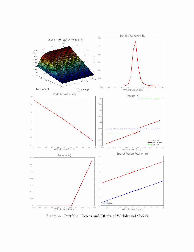
−0.5 −0.4 −0.3 −0.2 −0.1 0 0.1 0.2 0.3 0.40

0.002

0.004

0.006

0.008

0.01

0.012

Withdrawal Shock

Density Function (b)

−1 −0.8 −0.6 −0.4 −0.2 0 0.2 0.4 0.6 0.8 10.94

0.96

0.98

1

1.02

1.04

1.06

Withdrawal Shock

Portfolio Return (c)

−0.25 −0.2 −0.15 −0.1 −0.05 0 0.05 0.1 0.15 0.2 0.250.999

0.9995

1

1.0005

1.001

1.0015

1.002

1.0025

1.003

Withdrawal Shock

Returns (d)

Return loanReturn depositsReturn cash

−0.25 −0.2 −0.15 −0.1 −0.05 0 0.05 0.1 0.15 0.2 0.250

0.002

0.004

0.006

0.008

0.01

0.012

0.014

Withdrawal Shock

Penalty (e)

−1 −0.8 −0.6 −0.4 −0.2 0 0.2 0.4 0.6 0.8 1−60

−40

−20

0

20

40

60

Withdrawal Shock

End of Period Position (f)

CashDeposits

Figure 22: Portfolio Choices and Effects of Withdrawal Shocks

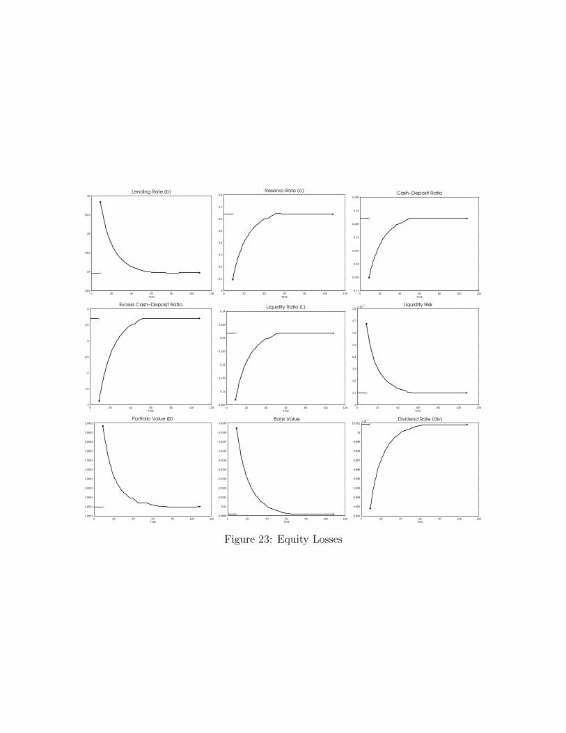
0 20 40 60 80 100 12023.5

24

24.5

25

25.5

26

Time

Lending Rate (b)

0 20 40 60 80 100 1203

3.1

3.2

3.3

3.4

3.5

3.6

3.7

3.8

Time

Reserve Rate (c)

0 20 40 60 80 100 1200.11

0.115

0.12

0.125

0.13

0.135

0.14

0.145

Time

Cash−Deposit Ratio

0 20 40 60 80 100 1201

1.5

2

2.5

3

3.5

4

Time

Excess Cash−Deposit Ratio

0 20 40 60 80 100 1200.105

0.11

0.115

0.12

0.125

0.13

0.135

0.14

Time

Liquidity Ratio (L)

0 20 40 60 80 100 1201

1.1

1.2

1.3

1.4

1.5

1.6

1.7

1.8x 10

−3

Time

Liquidity Risk

0 20 40 60 80 100 1201.0001

1.0001

1.0001

1.0001

1.0001

1.0001

1.0001

1.0002

1.0002

1.0002

1.0002

Time

Portfolio Value (Ω)

0 20 40 60 80 100 1200.0099

0.01

0.0101

0.0102

0.0103

0.0104

0.0105

0.0106

0.0107

0.0108

0.0109

Time

Bank Value

0 20 40 60 80 100 1209.991

9.992

9.993

9.994

9.995

9.996

9.997

9.998

9.999

10

10.001x 10

−3

Time

Dividend Rate (div)

Figure 23: Equity Losses

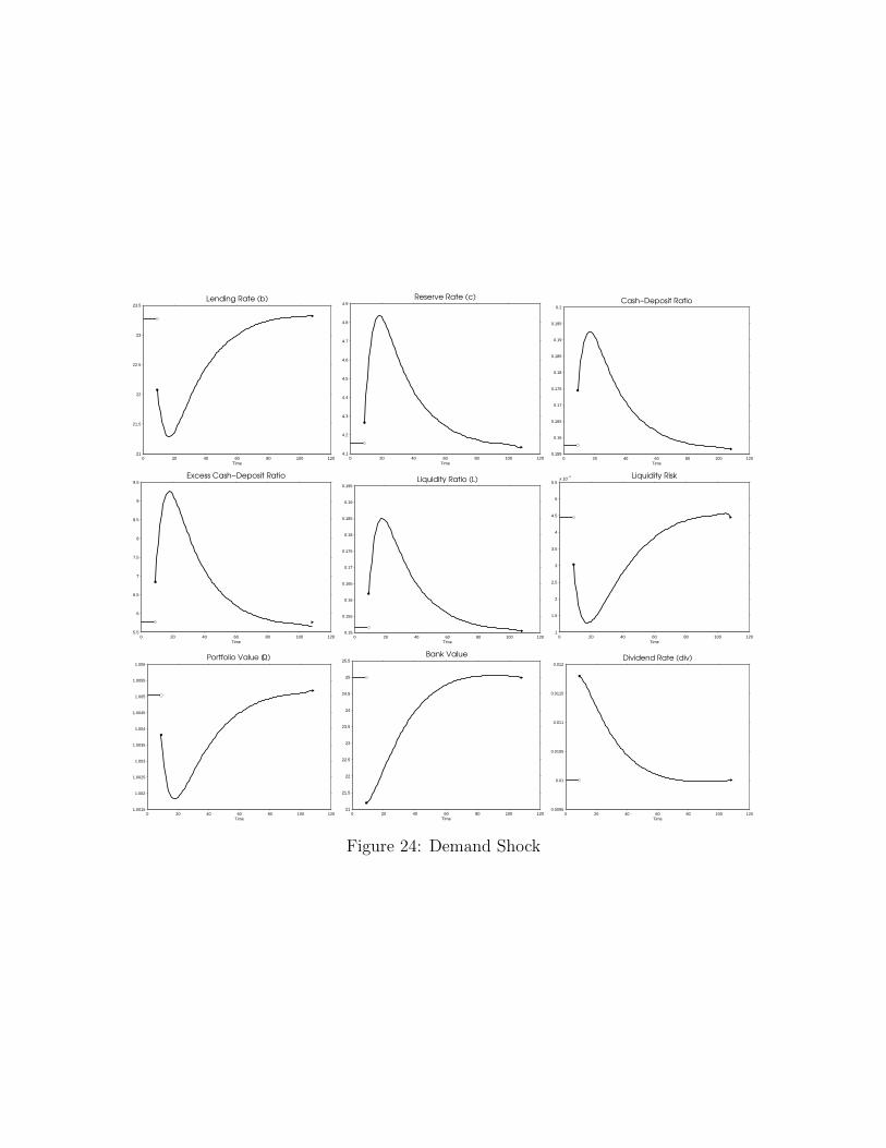
0 20 40 60 80 100 12021

21.5

22

22.5

23

23.5

Time

Lending Rate (b)

0 20 40 60 80 100 1204.1

4.2

4.3

4.4

4.5

4.6

4.7

4.8

4.9

Time

Reserve Rate (c)

0 20 40 60 80 100 1200.155

0.16

0.165

0.17

0.175

0.18

0.185

0.19

0.195

0.2

Time

Cash−Deposit Ratio

0 20 40 60 80 100 1205.5

6

6.5

7

7.5

8

8.5

9

9.5

Time

Excess Cash−Deposit Ratio

0 20 40 60 80 100 1200.15

0.155

0.16

0.165

0.17

0.175

0.18

0.185

0.19

0.195

Time

Liquidity Ratio (L)

0 20 40 60 80 100 1201

1.5

2

2.5

3

3.5

4

4.5

5

5.5x 10

−4

Time

Liquidity Risk

0 20 40 60 80 100 1201.0015

1.002

1.0025

1.003

1.0035

1.004

1.0045

1.005

1.0055

1.006

Time

Portfolio Value (Ω)

0 20 40 60 80 100 12021

21.5

22

22.5

23

23.5

24

24.5

25

25.5

Time

Bank Value

0 20 40 60 80 100 1200.0095

0.01

0.0105

0.011

0.0115

0.012

Time

Dividend Rate (div)

Figure 24: Demand Shock

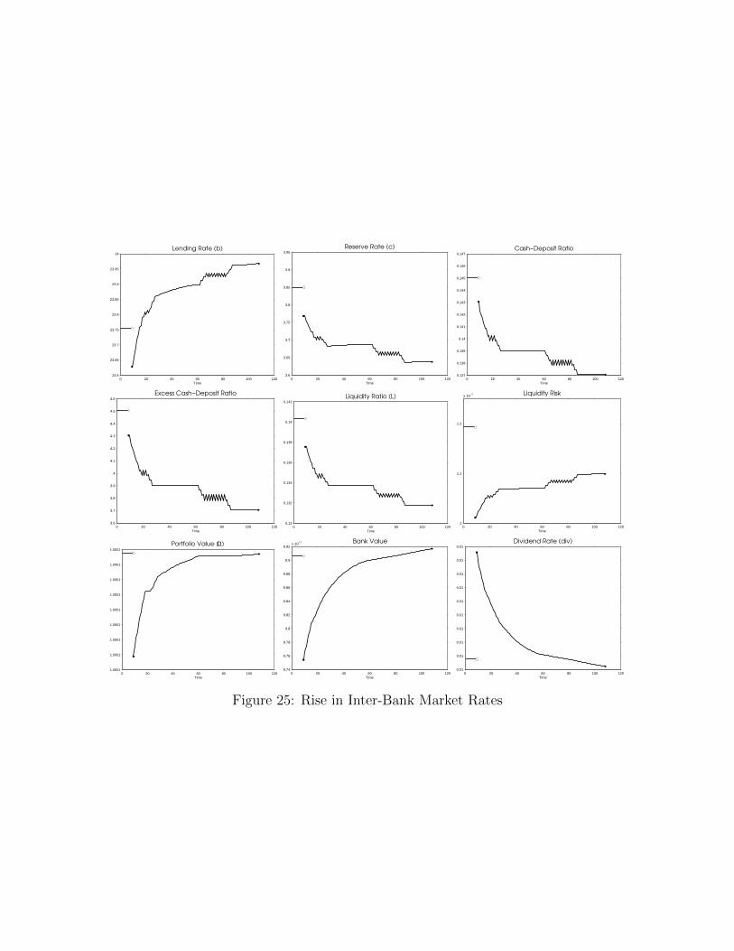
0 20 40 60 80 100 12023.6

23.65

23.7

23.75

23.8

23.85

23.9

23.95

24

Time

Lending Rate (b)

0 20 40 60 80 100 1203.6

3.65

3.7

3.75

3.8

3.85

3.9

3.95

Time

Reserve Rate (c)

0 20 40 60 80 100 1200.137

0.138

0.139

0.14

0.141

0.142

0.143

0.144

0.145

0.146

0.147

Time

Cash−Deposit Ratio

0 20 40 60 80 100 1203.6

3.7

3.8

3.9

4

4.1

4.2

4.3

4.4

4.5

4.6

Time

Excess Cash−Deposit Ratio

0 20 40 60 80 100 1200.13

0.132

0.134

0.136

0.138

0.14

0.142

Time

Liquidity Ratio (L)

0 20 40 60 80 100 1201

1.1

1.2

x 10−3

Time

Liquidity Risk

0 20 40 60 80 100 1201.0001

1.0001

1.0001

1.0001

1.0001

1.0001

1.0001

1.0001

1.0001

Time

Portfolio Value (Ω)

0 20 40 60 80 100 1209.74

9.76

9.78

9.8

9.82

9.84

9.86

9.88

9.9

9.92x 10

−3

Time

Bank Value

0 20 40 60 80 100 1200.01

0.01

0.01

0.01

0.01

0.01

0.01

0.01

0.01

0.01

Time

Dividend Rate (div)

Figure 25: Rise in Inter-Bank Market Rates

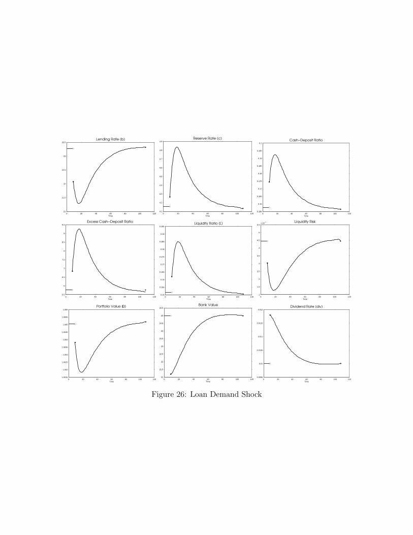
0 20 40 60 80 100 12021

21.5

22

22.5

23

23.5

Time

Lending Rate (b)

0 20 40 60 80 100 1204.1

4.2

4.3

4.4

4.5

4.6

4.7

4.8

4.9

Time

Reserve Rate (c)

0 20 40 60 80 100 1200.155

0.16

0.165

0.17

0.175

0.18

0.185

0.19

0.195

0.2

Time

Cash−Deposit Ratio

0 20 40 60 80 100 1205.5

6

6.5

7

7.5

8

8.5

9

9.5

Time

Excess Cash−Deposit Ratio

0 20 40 60 80 100 1200.15

0.155

0.16

0.165

0.17

0.175

0.18

0.185

0.19

0.195

Time

Liquidity Ratio (L)

0 20 40 60 80 100 1201

1.5

2

2.5

3

3.5

4

4.5

5

5.5x 10

−4

Time

Liquidity Risk

0 20 40 60 80 100 1201.0015

1.002

1.0025

1.003

1.0035

1.004

1.0045

1.005

1.0055

1.006

Time

Portfolio Value (Ω)

0 20 40 60 80 100 12021

21.5

22

22.5

23

23.5

24

24.5

25

25.5

Time

Bank Value

0 20 40 60 80 100 1200.0095

0.01

0.0105

0.011

0.0115

0.012

Time

Dividend Rate (div)

Figure 26: Loan Demand Shock

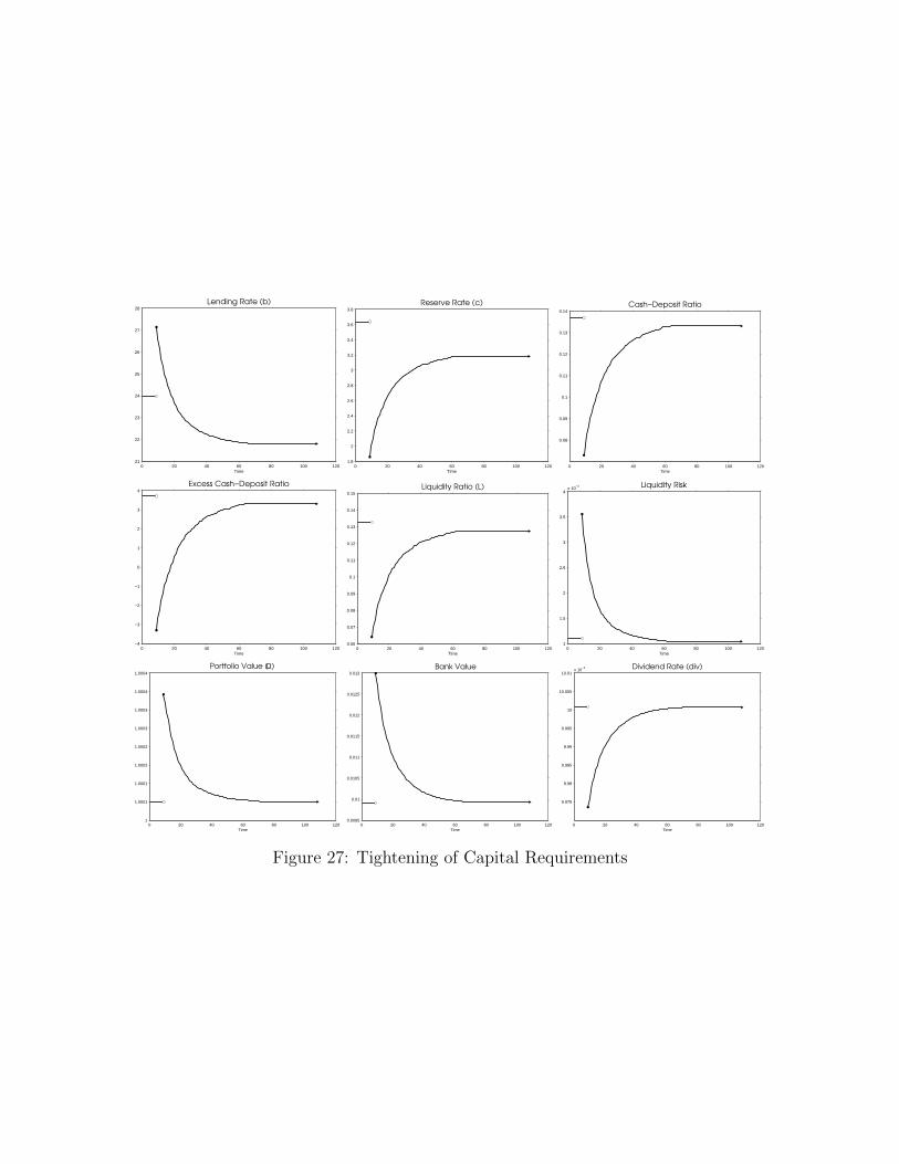
0 20 40 60 80 100 12021

22

23

24

25

26

27

28

Time

Lending Rate (b)

0 20 40 60 80 100 1201.8

2

2.2

2.4

2.6

2.8

3

3.2

3.4

3.6

3.8

Time

Reserve Rate (c)

0 20 40 60 80 100 120

0.08

0.09

0.1

0.11

0.12

0.13

0.14

Time

Cash−Deposit Ratio

0 20 40 60 80 100 120−4

−3

−2

−1

0

1

2

3

4

Time

Excess Cash−Deposit Ratio

0 20 40 60 80 100 1200.06

0.07

0.08

0.09

0.1

0.11

0.12

0.13

0.14

0.15

Time

Liquidity Ratio (L)

0 20 40 60 80 100 1201

1.5

2

2.5

3

3.5

4x 10

−3

Time

Liquidity Risk

0 20 40 60 80 100 1201

1.0001

1.0001

1.0002

1.0002

1.0003

1.0003

1.0004

1.0004

Time

Portfolio Value (Ω)

0 20 40 60 80 100 1200.0095

0.01

0.0105

0.011

0.0115

0.012

0.0125

0.013

Time

Bank Value

0 20 40 60 80 100 120

9.975

9.98

9.985

9.99

9.995

10

10.005

10.01x 10

−3

Time

Dividend Rate (div)

Figure 27: Tightening of Capital Requirements

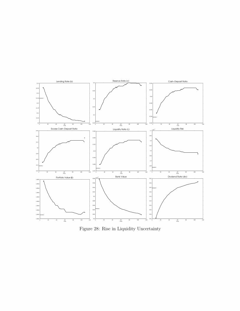
0 20 40 60 80 100 12021

21.05

21.1

21.15

21.2

21.25

21.3

21.35

21.4

Time

Lending Rate (b)

0 20 40 60 80 100 1206.15

6.2

6.25

6.3

6.35

6.4

Time

Reserve Rate (c)

0 20 40 60 80 100 1200.232

0.234

0.236

0.238

0.24

0.242

0.244

Time

Cash−Deposit Ratio

0 20 40 60 80 100 12013.2

13.4

13.6

13.8

14

14.2

14.4

14.6

Time

Excess Cash−Deposit Ratio

0 20 40 60 80 100 1200.224

0.226

0.228

0.23

0.232

0.234

0.236

Time

Liquidity Ratio (L)

0 20 40 60 80 100 1201.3

1.35

1.4

1.45

1.5

1.55

1.6

1.65

1.7x 10

−3

Time

Liquidity Risk

0 20 40 60 80 100 1201.0001

1.0001

1.0001

1.0001

1.0001

1.0001

1.0001

1.0001

1.0001

1.0001

Time

Portfolio Value (Ω)

0 20 40 60 80 100 1209.8

9.82

9.84

9.86

9.88

9.9

9.92

9.94

9.96

9.98x 10

−3

Time

Bank Value

0 20 40 60 80 100 1200.01

0.01

0.01

0.01

0.01

0.01

0.01

0.01

0.01

0.01

Time

Dividend Rate (div)

Figure 28: Rise in Liquidity Uncertainty

10.1 The Real Side - Closing the Model

We now turn to the real side of the model which is deliberately stylized. The idea is to

present an environment where there is a real demand for loans, without complicating the

analysis much. We make assumptions such that lending will have real effects despite that

the model has no nominal rigidities. Thus, monetary policy carries out real effects in a fully

real environment. In terms of the model, the goal here is to obtain a demand for loans like

the one in (6).

Thus, the economy is composed of an discrete infinite amount of islands, indexed by τ .

Each island is populated by workers and entrepreneurs. Islands are discovered in period τ .

Workers. Workers choose consumption, labor and deposit holdings. Workers don’t have

access to any additional savings technologies. Their period utility is given by:

maxctt≥0≥0,h0≥0

∞∑t=0

ct −(ht)

1+ν

(1 + ν)

where h0 is the labor supply and c consumption and ν is the inverse of the Frisch elasticity.

The worker’s budget constraint in period t is given by:

dwt+1 + ptct = dwt + wtht

where dwt+1 is the deposits held by the worker in period t, wt is the wage and pt the price

of the good. It is the case that dwt = 0, for all t ≤ τ. Workers only work during the period

of discovery τ , so without loss of generality ht = 0 for t 6= τ . The only role for workers is

to provide the elastic labor-supply schedule. The only reason why they are long-lived is to

allow us to talk about maturity in this model. Since deposits must be cleared out slowly,

household’s are long-lived. Also, notice that household’s don’t discount consumption over

time. This is enough to argue that they are indifferent between consumption in any period

so long as the price is constant. This allows us to eliminate any form of price variation in

the model together with zero interest on reserves.16

Problem 4 (Workers) The worker solves:

Uwt (τ, dwt ) = max

ct,htct −

(ht)1+ν

(1 + ν)+ Uw

t+1

(τ, dwt+1

)subject to

dwt+1 + ptct = dwt + wtht

16The model could be modified to allow workers to save. With GHH preferences, this would not alter thelabor supply. However, the model would require and additional state variable but the substance of the modelwould not change. GHH are commonly used to prevent counterfactual contractions in the labor supply.

with dw0 = 0, and ht = 0, for t 6= τ.

Entrepreneurs. Entrepreneurs have utility

maxctt≥0≥0

∞∑t=0

ct

They start their lives with a capital stock of kt. In addition, the have access to a loan market.

Their budget constraint in period t is given by:

ptct = retkt.

Production Technology. Production is carried out via k, combined with labor, h, using

a Cobb-Douglas technology F (k, h) ≡ kαh(1−α) to produce output. Profits are AF (k, h) −wh. Workers are hired from an elastic supply schedule, w = (hw)ν determined from the

worker’s problem.

Before production, an entrepreneur hires an amount of labor promising to pay wl. It

is possible that the entrepreneur reneges on this promise and defaults on his entire payroll.

This enforcement problem is not present between banks and firms. In particular, banks

can fully enforce their loan contracts. The lack of commitment between firms and workers

induces a financial need by firms. Firms can borrow from banks to finance payroll, issuing

a liability to the banking sector, whereas banking institutions take liabilities in the form of

deposit accounts with their workers.

Production is distributed over time via the following relationship. yt = (1− δ) δt−τReτ

where Reτ is the production per entrepreneur in island τ.

This delivers a problem for banks similar to Christiano and Eichenbaum (1992). This

problem is given by:

Problem 5 (Producer) The entrepreneur solves:

Reτ

(k; qlt, wt

)= max

l,hAkαh1−α − wth− (l − qltl)

subject to:(1− tax)wth ≤ qltl (8)

In this problem, ql is the amount of deposits (or credit) available to the firm. The firm

uses this credit is used to finance the payroll of the firm. The tax allows us to introduce a

labor market distortion that affects the real demand for loans. The solution to this problem

is given by:

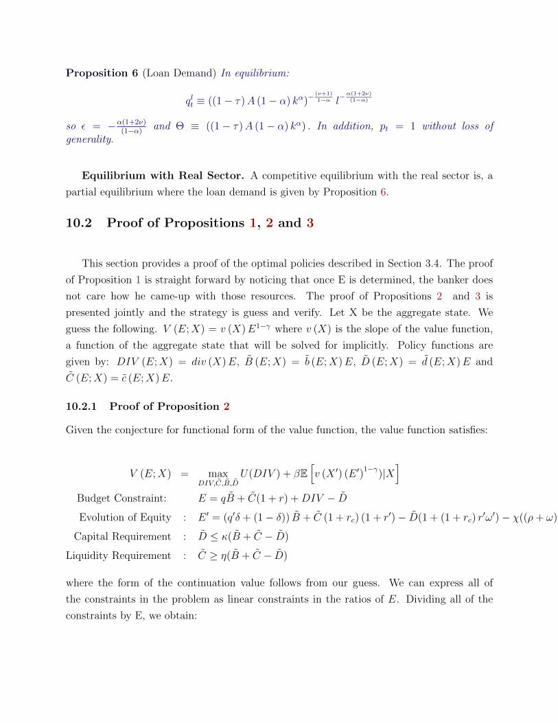
Proposition 6 (Loan Demand) In equilibrium:

qlt ≡ ((1− τ)A (1− α) kα)−(ν+1)1−α l−

α(1+2ν)(1−α)

so ε = −α(1+2ν)(1−α)

and Θ ≡ ((1− τ)A (1− α) kα) . In addition, pt = 1 without loss ofgenerality.

Equilibrium with Real Sector. A competitive equilibrium with the real sector is, a

partial equilibrium where the loan demand is given by Proposition 6.

10.2 Proof of Propositions 1, 2 and 3

This section provides a proof of the optimal policies described in Section 3.4. The proof

of Proposition 1 is straight forward by noticing that once E is determined, the banker does

not care how he came-up with those resources. The proof of Propositions 2 and 3 is

presented jointly and the strategy is guess and verify. Let X be the aggregate state. We

guess the following. V (E;X) = v (X)E1−γ where v (X) is the slope of the value function,

a function of the aggregate state that will be solved for implicitly. Policy functions are

given by: DIV (E;X) = div (X)E, B (E;X) = b (E;X)E, D (E;X) = d (E;X)E and

C (E;X) = c (E;X)E.

10.2.1 Proof of Proposition 2

Given the conjecture for functional form of the value function, the value function satisfies:

V (E;X) = maxDIV,C,B,D

U(DIV ) + βE[v (X ′) (E ′)

1−γ)|X]

Budget Constraint: E = qB + C(1 + r) +DIV − D

Evolution of Equity : E ′ = (q′δ + (1− δ)) B + C (1 + rc) (1 + r′)− D(1 + (1 + rc) r′ω′)− χ((ρ+ ω) D − C))

Capital Requirement : D ≤ κ(B + C − D)

Liquidity Requirement : C ≥ η(B + C − D)

where the form of the continuation value follows from our guess. We can express all of

the constraints in the problem as linear constraints in the ratios of E. Dividing all of the

constraints by E, we obtain:

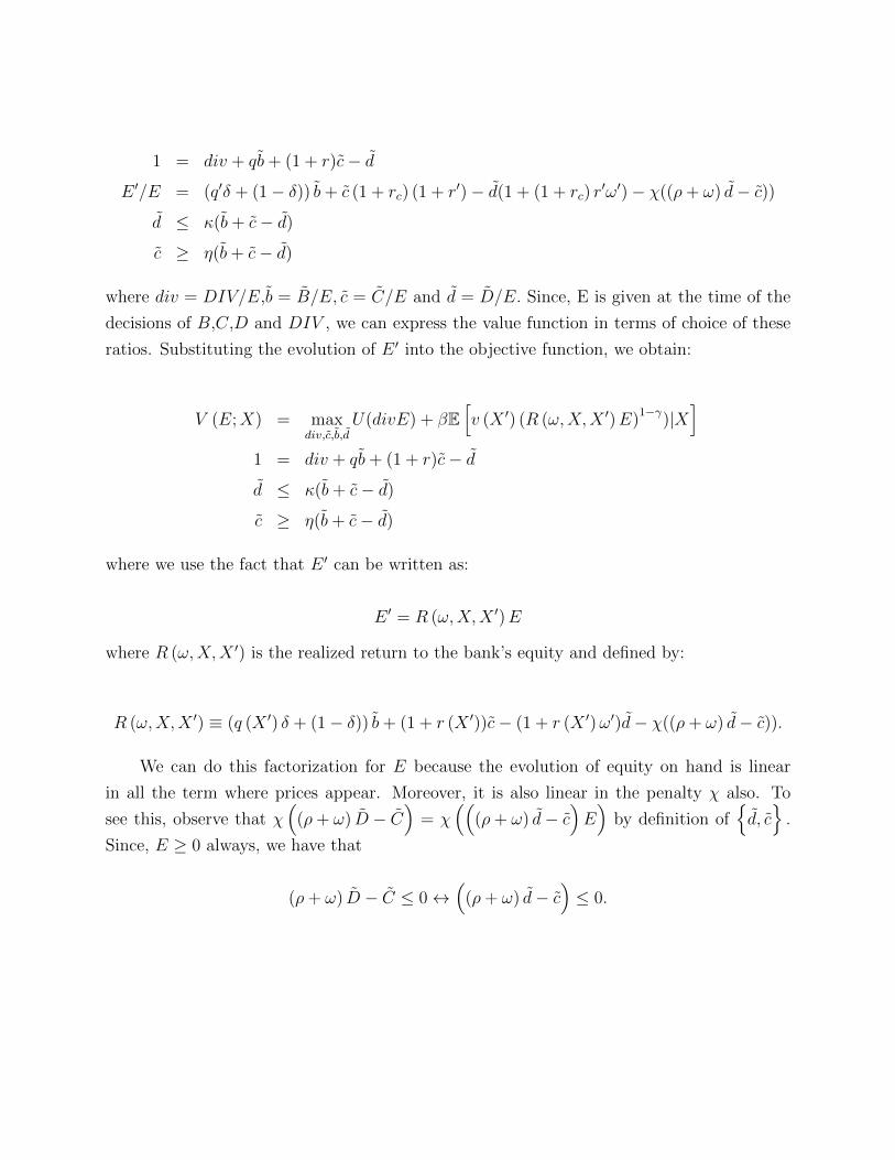
1 = div + qb+ (1 + r)c− d

E ′/E = (q′δ + (1− δ)) b+ c (1 + rc) (1 + r′)− d(1 + (1 + rc) r′ω′)− χ((ρ+ ω) d− c))

d ≤ κ(b+ c− d)

c ≥ η(b+ c− d)

where div = DIV/E,b = B/E, c = C/E and d = D/E. Since, E is given at the time of the

decisions of B,C,D and DIV , we can express the value function in terms of choice of these

ratios. Substituting the evolution of E ′ into the objective function, we obtain:

V (E;X) = maxdiv,c,b,d

U(divE) + βE[v (X ′) (R (ω,X,X ′)E)

1−γ)|X]

1 = div + qb+ (1 + r)c− d

d ≤ κ(b+ c− d)

c ≥ η(b+ c− d)

where we use the fact that E ′ can be written as:

E ′ = R (ω,X,X ′)E

where R (ω,X,X ′) is the realized return to the bank’s equity and defined by:

R (ω,X,X ′) ≡ (q (X ′) δ + (1− δ)) b+ (1 + r (X ′))c− (1 + r (X ′)ω′)d− χ((ρ+ ω) d− c)).

We can do this factorization for E because the evolution of equity on hand is linear

in all the term where prices appear. Moreover, it is also linear in the penalty χ also. To

see this, observe that χ(

(ρ+ ω) D − C)

= χ((

(ρ+ ω) d− c)E)

by definition ofd, c.

Since, E ≥ 0 always, we have that

(ρ+ ω) D − C ≤ 0↔(

(ρ+ ω) d− c)≤ 0.

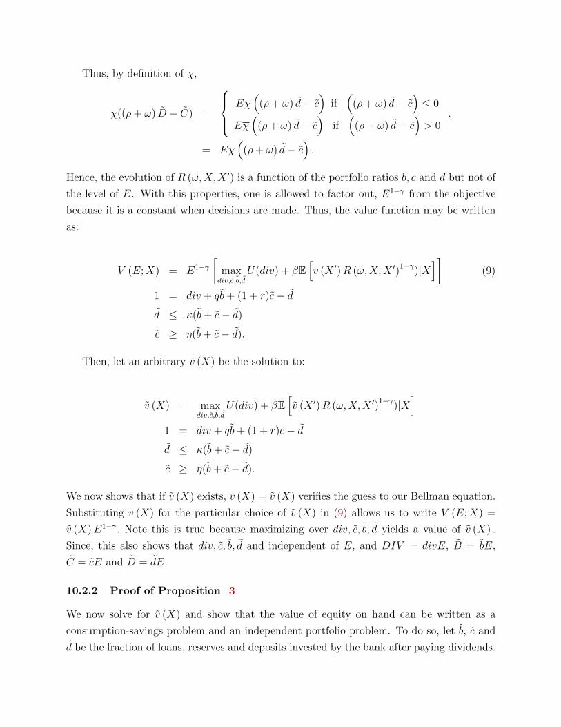
Thus, by definition of χ,

χ((ρ+ ω) D − C) =

Eχ(

(ρ+ ω) d− c)

if(

(ρ+ ω) d− c)≤ 0

Eχ(

(ρ+ ω) d− c)

if(

(ρ+ ω) d− c)> 0

.

= Eχ(

(ρ+ ω) d− c).

Hence, the evolution of R (ω,X,X ′) is a function of the portfolio ratios b, c and d but not of

the level of E. With this properties, one is allowed to factor out, E1−γ from the objective

because it is a constant when decisions are made. Thus, the value function may be written

as:

V (E;X) = E1−γ[

maxdiv,c,b,d

U(div) + βE[v (X ′)R (ω,X,X ′)

1−γ)|X]]

(9)

1 = div + qb+ (1 + r)c− d

d ≤ κ(b+ c− d)

c ≥ η(b+ c− d).

Then, let an arbitrary v (X) be the solution to:

v (X) = maxdiv,c,b,d

U(div) + βE[v (X ′)R (ω,X,X ′)

1−γ)|X]

1 = div + qb+ (1 + r)c− d

d ≤ κ(b+ c− d)

c ≥ η(b+ c− d).

We now shows that if v (X) exists, v (X) = v (X) verifies the guess to our Bellman equation.

Substituting v (X) for the particular choice of v (X) in (9) allows us to write V (E;X) =

v (X)E1−γ. Note this is true because maximizing over div, c, b, d yields a value of v (X) .

Since, this also shows that div, c, b, d and independent of E, and DIV = divE, B = bE,

C = cE and D = dE.

10.2.2 Proof of Proposition 3

We now solve for v (X) and show that the value of equity on hand can be written as a

consumption-savings problem and an independent portfolio problem. To do so, let b, c and

d be the fraction of loans, reserves and deposits invested by the bank after paying dividends.

To simplify notation, we suppress the reference to the aggregate state X. These functions

are mathematically defined as:

b ≡ b

(1− div), c ≡ c

(1− div)and d ≡ d

(1− div).

and collecting terms we obtain:

div + (1− div)(qb+ (1 + r)c− d

)= 1.

Thus, the resource constraint for the bank can also be written as,

qb+ (1 + r)c− d = 1.

Similarly, we can multiply the capital and liquidity constraints by (1− div) and express the

constraints in :

d ≤ κ(b+ c− d)

c ≥ η(b+ c− d).

To make further progress, we employ the principle of optimality and solve forb, c, d

,

assuming we already know div. Let’s assume an arbitrary divo as the optimal choice in

v (X). Then v (X) also satisfies:

v (X) = maxb,c,d

U(divo) + (1− divo)1−γ βE[v (X ′)R (ω,X,X ′)

1−γ)|X]

subject to:

1 = qb+ c(1 + r)− d

d ≤ κ(b+ c− d)

c ≥ η(b+ c− d).

We note thatR (ω,X,X ′) = (q (X ′) δ + (1− δ)) b+(1+r (X ′))c−(1+r (X ′)ω′)d−χ((ρ+ ω) d−c)) (1− divo) . SinceR (ω,X,X ′) only enterers in the continuation utility, then,

b, c, d

must

solve:

maxb,c,d

E[v (X ′) (q (X ′) δ + (1− δ)) b+ (1 + r (X ′))c− d(1 + r (X ′)ω′)− χ((ρ+ ω) d− c))1−γ)|X

].

subject to

1 = qb+ c(1 + r)− d

d ≤ κ(b+ c− d)

c ≥ η(b+ c− d)

if it is part of a solution, otherwise there is a better solution to v (X).

When, X ′ is deterministic v (X ′) is know at stage X. In such cases, we can factor out this

problem out of the max. However, we must be careful with the sign of v (X ′) since the max

operator switches to a min operator when we change signs. We will show that when γ > 1,

v (X ′) is negative, so we need to minimize term inside the brackets. To prevent changing the

max operator to a min operator, we use the certainty equivalent operator. Thus,b, c, d

are solutions to:

Ω (X) = maxb,c,d

Eω[(q (X ′) δ + (1− δ)) b+ (1 + r (X ′))c− d(1 + r (X ′)ω′)− χ((ρ+ ω) d− c))1−γ)

] 11−γ

.

subject to

1 = qb+ c(1 + r)− d

d ≤ κ(b+ c− d)

c ≥ η(b+ c− d).

When, (1− γ) < 0, the solution to Ω (X) will be equivalent to minimizing the objective. For

γ → 1, the objective becomes:

Ω (X) = exp Eω [log (R (ω,X,X ′))] .

Note that we can only do this separation when X is deterministic because otherwise we need

to account for the correlation between v (X ′) and R (ω,X,X ′) . However, for now we assume

the problem is deterministic. Since, the solution to Ω (X) is the same for any div, and not

just the optimal, divo. The objective can be written as

v (X) = maxdiv

U(div) + (1− div)1−γ βE[v (X ′) Ω (X)1−γ)|X

],

which is the formulation in Proposition 3. Proposition 5 shows an explicit solution for div

and v (X) .

10.3 Equivalence in Problems

We now show that using our guessed policy functions we recover the consumption savings

problem above. In the original problem, the first order conditions for b is:

(b)

: q (X)U′(div (X)E)E = β

(E[v (X)u′ (E ′)

∂E ′

∂b

])+ µκ (X)E1−γκ− µη (X)E1−γη.

(10)

Now, we know from xxx that ∂E′

∂bis:

(q (X ′) δ + (1− δ))E.

Hence, the first order condition becomes:

q (X)U′(div (X))E1−γ = βE [v (X)u′ (R (ω,X,X ′)E) (q (X ′) δ + (1− δ))E]+µκ (X)E1−γκ−µη (X)E1−γη,

and simplifying E this equation further more, we obtain:

q (X)U′(div (X)) = βE

[v (X)R (ω,X,X ′)

−γ(q (X ′) δ + (1− δ))

]+ µκ (X)κ− µη (X) η.

Similarly, the first order condition for c (X) yields,

(c) : (1+r (X))U′(div (X)) = βE

[v (X)R (ω,X,X ′)

−γ ∂R (ω,X,X ′)

∂c

]+µκ (X)κ−µη (X) (η − 1) ,

(11)

and a similar expression can be found for d (X) :

(d)

: U′(div (X)) = βE

[v (X)R (ω,X,X ′)

−γ ∂R (ω,X,X ′)

∂d

]+ µκ (X) (1− κ) + µη (X) η.

(12)

Note that 10, 11 and 12 are independent of E. One can multiply equation 10 by b, equation

11 by c and equation 12 by d, and obtain:

U′(div) = (1− div)1−γ βE

[v (X) Ω (X)1−γ]

To see this, note that we are using the definitions

µκ (X)[κ(b (E;X) + c (E;X)− d (E;X))− d (E;X)

]= 0

and

µη (X)[c (E;X)− η(b (E;X) + c (E;X)− d (E;X))

]= 0

and that qb+(1+r)c− d = 1. Since, U′(div) = (1− div)1−γ βE

[v (X) Ω (X)1−γ] is the same

first order condition for the for the problem in Proposition 5, we know that the optimal

dividend choice satisfies the conditions in that problem also.

10.4 Proof of Proposition 5

Taking first order conditions we obtain:

div = βE[vl (X ′) |X

]Ω∗ (X)−1/γ (1− div)

and therefore one obtains:

div =1

1 + [βE [vl (X ′) |X] Ω∗ (X)]1/γ.

Substituting this expression for dividends, one obtains a functional equation for the value

function:

vl (X) =1(

1 + [βE [vl (X ′) |X] Ω∗ (X)]1γ

)1−γ

+βE[vl (X ′) |X

]Ω∗ (X)

[βE[vl (X ′) |X

]Ω∗ (X)

] 1γ(

1 + [βE [vl (X ′) |X] Ω∗ (X)]1γ

)1−γ

=

1 +

([βE[vl (X ′) |X

]Ω∗ (X)

] γ+(1−γ)γ(1−γ)

)1−γ

(1 + [βE [vl (X ′) |X] Ω∗ (X)]

1γ

)1−γ

=

1 +[βE[vl (X ′) |X

]Ω∗ (X)

] 1γ(

1 + [βE [vl (X ′) |X] Ω∗ (X)]1γ

)1−γ

=

(1 +

[βE[vl (X ′) |X

]Ω∗ (X)

] 1γ

)γ

Therefore, we obtain the following map:

vl (X)1γ = 1 + (βΩ∗ (X))

1γ E[vl (X ′) |X

] 1γ .

Performing a change of variables, and denoting υ (X) ≡ vl (X)1γ , we have the following

functional equation:

υ (X) = 1 + (βΩ∗ (X))1γ E[υ (X ′)

γ |X] 1γ .

We can treat the right hand side of this functional equation as an operator. This operator

will be a contraction depending on the values of (βΩ∗ (X))1γ . Theorems in Alvarez and Stokey

guarantee that this operator satisfies the dynamic programming arguments.

In a non-stochastic steady state we obtain:

vl (X) =

(1

1− (βΩ∗ (X))1γ

)γ

.

11 Derivation of Loan Demand (Incomplete)

The firm maximizes production minus its acquired financial liabilities. Substituting the

constraint and taking first order conditions with respect to loans delivers:

A (1− α) kα(

qlt(1− τ)wt

)1−α

l−α = 1.

Now, one given the linearity of profits in bank loans per unit of capital, the total demand

for h is given by:

qltwtl = HD.

Hence, in equilibrium,

(qlt

(1− τ)wtl

)ν= wt →

(qltl

(1− τ)

) νν+1

= wt.

Back in the first order condition yields:

A (1− α) kα

(qlt

(1− τ)(qltl) νν+1

)1−α

l−α = 1.

and this returns:

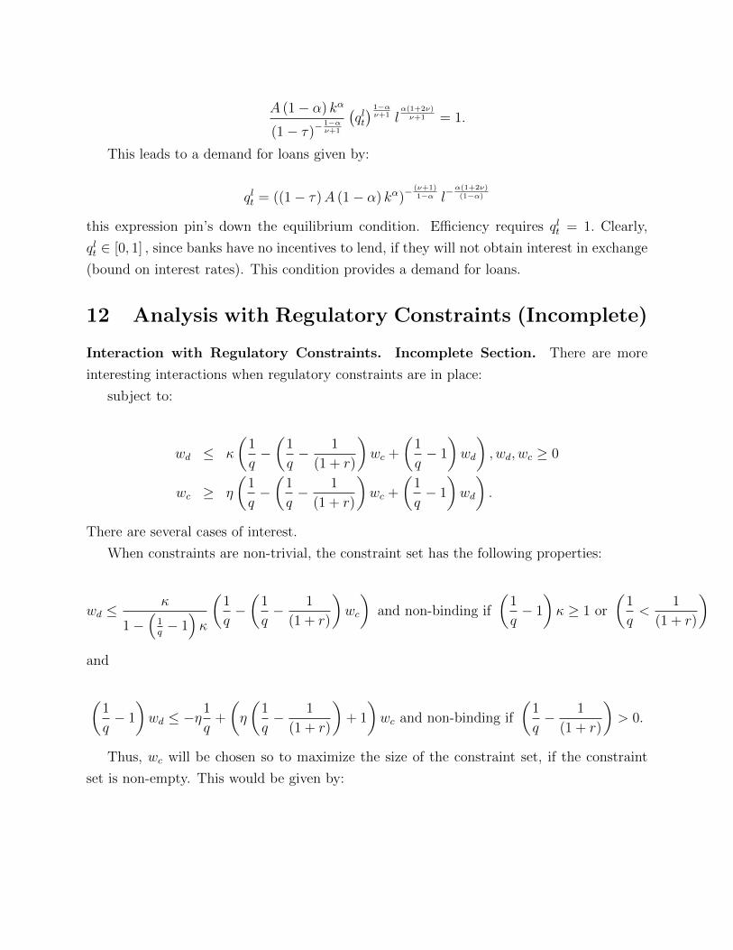
A (1− α) kα

(1− τ)−1−αν+1

(qlt) 1−αν+1 l

α(1+2ν)ν+1 = 1.

This leads to a demand for loans given by:

qlt = ((1− τ)A (1− α) kα)−(ν+1)1−α l−

α(1+2ν)(1−α)

this expression pin’s down the equilibrium condition. Efficiency requires qlt = 1. Clearly,

qlt ∈ [0, 1] , since banks have no incentives to lend, if they will not obtain interest in exchange

(bound on interest rates). This condition provides a demand for loans.

12 Analysis with Regulatory Constraints (Incomplete)

Interaction with Regulatory Constraints. Incomplete Section. There are more

interesting interactions when regulatory constraints are in place:

subject to:

wd ≤ κ

(1

q−(

1

q− 1

(1 + r)

)wc +

(1

q− 1

)wd

), wd, wc ≥ 0

wc ≥ η

(1

q−(

1

q− 1

(1 + r)

)wc +

(1

q− 1

)wd

).

There are several cases of interest.

When constraints are non-trivial, the constraint set has the following properties:

wd ≤κ

1−(

1q− 1)κ

(1

q−(

1

q− 1

(1 + r)

)wc

)and non-binding if

(1

q− 1

)κ ≥ 1 or

(1

q<

1

(1 + r)

)

and

(1

q− 1

)wd ≤ −η

1

q+

(η

(1

q− 1

(1 + r)

)+ 1

)wc and non-binding if

(1

q− 1

(1 + r)

)> 0.

Thus, wc will be chosen so to maximize the size of the constraint set, if the constraint

set is non-empty. This would be given by:

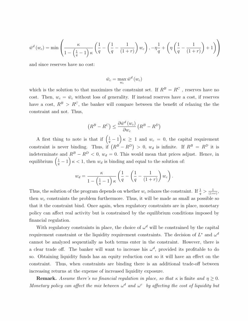
wd (wc) = min

κ

1−(

1q− 1)κ

(1

q−(

1

q− 1

(1 + r)

)wc

),−η1

q+

(η

(1

q− 1

(1 + r)

)+ 1

)and since reserves have no cost:

wc = maxwc

wd (wc)

which is the solution to that maximizes the constraint set. If RB = RC , reserves have no

cost. Then, wc = wc without loss of generality. If instead reserves have a cost, if reserves

have a cost, RB > RC , the banker will compare between the benefit of relaxing the the

constraint and not. Thus,

(RB −RC

)≤ ∂wd (wc)

∂wc

(RB −RD

)A first thing to note is that if

(1q− 1)κ ≥ 1 and wc = 0, the capital requirement

constraint is never binding. Thus, if(RB −RD

)> 0, wd is infinite. If RB = RD it is

indeterminate and RB − RD < 0, wd = 0. This would mean that prices adjust. Hence, in

equilibrium(

1q− 1)κ < 1, then wd is binding and equal to the solution of:

wd =κ

1−(

1q− 1)κ

(1

q−(

1

q− 1

(1 + r)

)wc

).

Thus, the solution of the program depends on whether wc relaxes the constraint. If 1q> 1

(1+r),

then wc constraints the problem furthermore. Thus, it will be made as small as possible so

that it the constraint bind. Once again, when regulatory constraints are in place, monetary

policy can affect real activity but is constrained by the equilibrium conditions imposed by

financial regulation.

With regulatory constraints in place, the choice of ωd will be constrained by the capital

requirement constraint or the liquidity requirement constraints. The decision of L∗ and ωd

cannot be analyzed sequentially as both terms enter in the constraint. However, there is

a clear trade off. The banker will want to increase his ωd, provided its profitable to do

so. Obtaining liquidity funds has an equity reduction cost so it will have an effect on the

constraint. Thus, when constraints are binding there is an additional trade-off between

increasing returns at the expense of increased liquidity exposure.

Remark. Assume there’s no financial regulation in place, so that κ is finite and η ≥ 0.

Monetary policy can affect the mix between ωd and ωc by affecting the cost of liquidity but

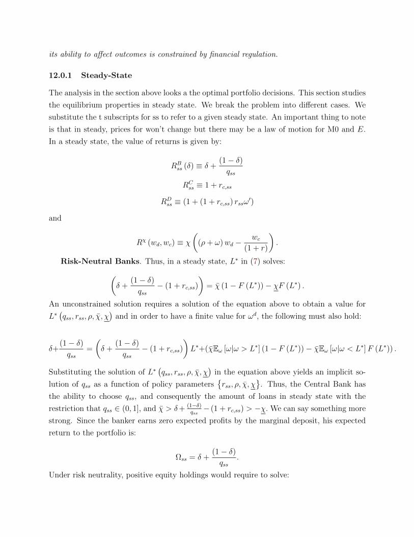
its ability to affect outcomes is constrained by financial regulation.

12.0.1 Steady-State

The analysis in the section above looks a the optimal portfolio decisions. This section studies

the equilibrium properties in steady state. We break the problem into different cases. We

substitute the t subscripts for ss to refer to a given steady state. An important thing to note

is that in steady, prices for won’t change but there may be a law of motion for M0 and E.

In a steady state, the value of returns is given by:

RBss (δ) ≡ δ +

(1− δ)qss

RCss ≡ 1 + rc,ss

RDss ≡ (1 + (1 + rc,ss) rssω

′)

and

Rχ (wd, wc) ≡ χ

((ρ+ ω)wd −

wc(1 + r)

).

Risk-Neutral Banks. Thus, in a steady state, L∗ in (7) solves:(δ +

(1− δ)qss

− (1 + rc,ss)

)= χ (1− F (L∗))− χF (L∗) .

An unconstrained solution requires a solution of the equation above to obtain a value for

L∗(qss, rss, ρ, χ, χ

)and in order to have a finite value for ωd, the following must also hold:

δ+(1− δ)qss

=

(δ +

(1− δ)qss

− (1 + rc,ss)

)L∗+(χEω [ω|ω > L∗] (1− F (L∗))− χEω [ω|ω < L∗]F (L∗)) .

Substituting the solution of L∗(qss, rss, ρ, χ, χ

)in the equation above yields an implicit so-

lution of qss as a function of policy parametersrss, ρ, χ, χ

. Thus, the Central Bank has

the ability to choose qss, and consequently the amount of loans in steady state with the

restriction that qss ∈ (0, 1], and χ > δ+ (1−δ)qss− (1 + rc,ss) > −χ. We can say something more

strong. Since the banker earns zero expected profits by the marginal deposit, his expected

return to the portfolio is:

Ωss = δ +(1− δ)qss

.

Under risk neutrality, positive equity holdings would require to solve:

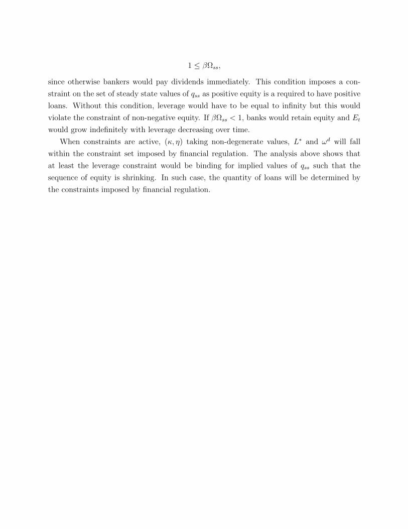
1 ≤ βΩss,

since otherwise bankers would pay dividends immediately. This condition imposes a con-

straint on the set of steady state values of qss as positive equity is a required to have positive

loans. Without this condition, leverage would have to be equal to infinity but this would

violate the constraint of non-negative equity. If βΩss < 1, banks would retain equity and Et

would grow indefinitely with leverage decreasing over time.

When constraints are active, (κ, η) taking non-degenerate values, L∗ and ωd will fall

within the constraint set imposed by financial regulation. The analysis above shows that

at least the leverage constraint would be binding for implied values of qss such that the

sequence of equity is shrinking. In such case, the quantity of loans will be determined by

the constraints imposed by financial regulation.