Finance and Economics Discussion SeriesDivisions of Research & Statistics and Monetary Affairs

Federal Reserve Board, Washington, D.C.

Customer Liquidity Provision: Implications for Corporate BondTransaction Costs

Jaewon Choi and Yesol Huh

2017-116

Please cite this paper as:Choi, Jaewon, and Yesol Huh (2017). “Customer Liquidity Provision: Implica-tions for Corporate Bond Transaction Costs,” Finance and Economics Discussion Se-ries 2017-116. Washington: Board of Governors of the Federal Reserve System,https://doi.org/10.17016/FEDS.2017.116.

NOTE: Staff working papers in the Finance and Economics Discussion Series (FEDS) are preliminarymaterials circulated to stimulate discussion and critical comment. The analysis and conclusions set forthare those of the authors and do not indicate concurrence by other members of the research staff or theBoard of Governors. References in publications to the Finance and Economics Discussion Series (other thanacknowledgement) should be cleared with the author(s) to protect the tentative character of these papers.

Customer Liquidity Provision:

Implications for Corporate Bond Transaction Costs∗

Jaewon Choi† Yesol Huh‡

First draft: July 2016

Current draft: October 2017

Abstract

The convention in calculating trading costs in corporate bond markets is to assume

that dealers provide liquidity to non-dealers (customers) and to calculate average bid-

ask spreads that customers pay dealers. We show that customers often provide liquidity

in corporate bond markets, and thus, average bid-ask spreads underestimate trading

costs that customers demanding liquidity pay. Since the periods before the 2008 fi-

nancial crisis, substantial amounts of liquidity provision have moved from the dealer

sector to the non-dealer sector, consistent with decreased dealer risk capacity. Among

trades where customers are demanding liquidity, we find that these customers pay 35

to 50 percent higher spreads than before the crisis. Our results indicate that liquidity

decreased in corporate bond markets and can help explain why, despite the decrease

in dealers’ risk capacity, average bid-ask spread estimates remain low.

∗Earlier drafts were circulated under the title “Customer Liquidity Provision in Corporate Bond Markets.”We are grateful to Scott Bauguess, Andrew Chen, Darrell Duffie, Erik Heitfield, Terrence Hendershott, EdithHotchkiss, Stacey Jacobsen, Yoshio Nozawa, Elvira Solji, Clara Vega, Brian Weller, and the conference andseminar participants at Bank of Canada, the CFTC, the SEC, 2017 CICF, 2017 European Finance Associa-tion Annual Meeting, Workshop on Investor Behavior and Market Liquidity, and Women in MicrostructureMeeting for their comments and discussions. The views expressed in this article are soley those of the authorsand should not be interpreted as reflecting the views of the Federal Reserve Board or the Federal ReserveSystem. Please send comments to yesol.huh@frb.gov.†Department of Finance, University of Illinois at Urbana-Champaign. Email: jaewchoi@illinois.edu.‡Federal Reserve Board. Email: yesol.huh@frb.gov.

1

1 Introduction

Whether corporate bond liquidity has deteriorated has been hotly debated amongst both

practitioners and academics since the introduction of new bank regulations such as the Vol-

cker Rule and more stringent capital regulations. Three broad findings have emerged from the

academic literature. First, dealers—especially those more heavily affected by various bank

regulations—have decreased capital commitment and liquidity provision (Bessembinder, Ja-

cobsen, Maxwell and Venkataraman (2017), Bao, O’Hara and Zhou (2017), and Schultz

(2017)). However, broad price-based measures of liquidity have not worsened (Trebbi and

Xiao (2017), Adrian, Fleming, Shachar and Vogt (2017), Anderson and Stulz (2017)). Fi-

nally, liquidity during specific market stress or liquidity events, such as rating downgrades

or index rebalancing, has worsened (Bao et al. (2017), Dick-Nielsen and Rossi (2016)).

These findings seem puzzling; given that corporate bond markets are dealer-intermediated,

we would expect market liquidity to worsen if dealers decrease their risk capacity. In this

paper, we provide an explanation that helps reconcile these findings: an increase in liquid-

ity provision by customers. In particular, we argue that bid-ask spreads are seemingly low

because average bid-ask spreads that customers pay are a biased measure of the true cost of

demanding liquidity. Using the regulatory version of the Trade Reporting and Compliance

Engine (TRACE) database of U.S. corporate bond transactions from 2006 to 2015, we show

that buy-side investors (“customers”) often provide liquidity and that this customer liquidity

provision causes our usual estimates of bid-ask spreads to underestimate the trading costs

paid by liquidity-demanding customers. Moreover, as dealers become less willing to take

inventory risk in the post-regulation period, customer liquidity provision increases, which

exacerbates the underestimation problem. Once we correct for this bias, the measured cost

of demanding liquidity is substantially higher during the post-regulation period compared

with the pre-crisis period. Thus, our results can help explain why the literature so far has

2

found that bid-ask spreads in the post-regulation periods are not higher despite decreased

dealer liquidity provision.

Liquidity provision by customers may cause observed bid-ask spreads to underestimate

the true cost of liquidity demand. Suppose a customer (C1) wants to sell a bond and contacts

a dealer. The dealer, due to limited risk-taking capacity, is willing to take inventory risk

only by charging substantial spreads (for example, 30 basis points (bps)). Instead of finding

someone with a liquidity need to buy the bond, the dealer might find a non-dealer (C2) who

is willing to provide liquidity for a fee (i.e., buying at a lower price than the fundamental

value of the bond) even without a strict liquidity need. In this scenario, C1 is demanding

liquidity, and C2 is providing liquidity. Also, C1 sells at a higher price than she would

without liquidity provision by C2, because the dealer is willing to charge a spread smaller

than 30 bps as the dealer does not take on inventory risk. C2 pays an even smaller spread (a

negative spread in this scenario), implying that the average bid-ask spread paid by the two

customers is much lower than the spread that would be paid by a customer that demanded

immediacy. For instance, if C1 pays the dealer 10 bps and the dealer pays 4 bps to C2 (i.e.,

dealer sells to C2 at 4 bps lower than the fundamental price), then the average bid-ask spread

is (10− 4)/2 = 3 bps, which is lower than the 30 bps that a customer demanding immediacy

will pay and also lower than the 10 bps that C1 paid. Importantly, the transaction between

a dealer and a liquidity-providing customer can occur at a lower price than the fundamental

value, indicating that the spread can be negative. Furthermore, the amounts of customer

liquidity provision can be measured by the fraction of two matched customer trades (DC-DC

trades, henceforth).

To the extent that customers exploit increased spreads quoted by dealers, customer liq-

uidity provision will become stronger and underestimation of the true cost of immediacy will

be more severe as dealers face increased inventory costs. Suppose that dealers face higher

inventory costs and increases the price for immediate execution to 40 bps. Some customers

3

that would have traded immediately with a dealer (and paid 30 bps) decide to wait for the

dealer to find a counterparty, and some other customers may decide not to trade altogether,

because transaction costs would be too high. The dealer will actively search for liquidity-

providing customers, as matching trades with a liquidity-providing customer is better than

foregoing a transaction with a liquidity-seeking seller. Thus, the fraction of DC-DC matched

trades increases, and a higher fraction of liquidity is essentially provided by non-dealers.

Moreover, despite the increased cost of immediacy, the average bid-ask spread paid by all

customers may remain similar or even decrease due to the shift in the composition of liquidity

provision between dealers and customers. We also expect this effect to be asymmetric and

stronger when liquidity-providing customers buy, as large asset managers are increasingly

stepping in to provide liquidity in the post-regulation period.1 It is relatively easier for such

asset managers to provide liquidity on their long positions, as they typically should hold net

long positions and also have been receiving substantial amounts of investor flows during the

post-crisis period.

Our main database, the regulatory TRACE, provides dealer identities for each reported

trade, which allows us to identify DC-DC trades and thus measure the degrees of customer

liquidity provision. In particular, we match a trade between a customer and dealer with an

offsetting trade between the same dealer and another customer (i.e., matching a buy with

a sell and vice versa), using a last-in-first-out (LIFO) algorithm. We categorize as a DC-

DC trade a customer trade that is matched to another customer trade within the next 15

minutes. As outlined previously, we hypothesize that these trades are generally one customer

demanding liquidity and another customer supplying liquidity. Similarly, we define DC-ID

1For example, BlackRock, a large institutional asset manager, commented that it is not only a pricetaker, but now also acts as a “price maker” that “expresses a price at which he or she is willing to buy(or sell) a particular security at a given time” (BlackRock (2015)). Also, a recent Wall Street Journalarticle mentions that “giant bond firms increasingly are taking on a price setting role in global debt mar-kets, elbowing aside big banks facing tighter post-crisis regulation”. (https://www.wsj.com/articles/in-the-new-bond-market-bigger-is-better-1498046401)

4

trades, which are customer trades matched with offsetting interdealer trades within the 15

minute window. These DC-ID matches are likely driven by a customer demanding liquidity

and the other matched dealer providing liquidity. Trades that remain in dealers’ inventory

for longer than 15 minutes are categorized as invt>15min trades.

We provide empirical evidence that is consistent with predictions implied by customer

liquidity provision. First, we show that customer trades that are matched with other cus-

tomer trades (i.e., DC-DC trades) have lower average spreads than customer trades that are

not matched. We find that DC-DC trades have 20–40% lower bid-ask spreads compared with

trades where customers are demanding liquidity, indicating that average bid-ask spreads un-

derestimate trading costs for customers demanding liquidity. We find that 40% of DC-DC

trades exhibit negative spreads, higher than that of DC-ID or invt>15min trades. Further-

more, DC-DC trades have lower bid-ask spreads and are more likely to have negative spreads

particularly for customer buy trades, which is consistent with our prediction that customers

have more capacity to provide liquidity on their long positions. For investment grade bonds,

for example, DC-DC trades for customer buys (sells) are on average 42.6 (23.7) bps and

17.17 (6.6) bps lower than DC-ID and invt>15min customer buy (sell) trades, respectively.

Also, we find that the bid-ask spreads for DC-DC trades are lower particularly for bonds

that trade infrequently, consistent with our customer liquidity provision hypothesis in that

liquidity-providing customers are compensated more for bonds with high dealer inventory

risk.

Next, we also show that this underestimation problem is severe for commonly used mea-

sures of bid-ask spreads in the literature, namely, the implied roundtrip costs of Feldhutter

(2012) and the bid-ask spread estimates based on differences in customer buy and sell prices

used in Hong and Warga (2000) and Adrian, Fleming, Shachar and Vogt (2017). These

measures implicitly treat DC-DC trades as customer trades seeking immediacy and also

put higher weights on those trades. More generally, a bid-ask spread measure would tend

5

to understate the true cost of liquidity demand to the extent that it puts more weight in

short-horizon trades, as our results show that liquidity provision is concentrated the most in

short-horizon customer trades.

Lastly, we examine the extent to which increasing customer liquidity provision as proxied

by DC-DC matched trades can explain the seemingly low transaction costs in the corporate

bond market. We show that in the post-regulation period, compared with the pre-crisis

period, dealers match a higher fraction of customer trades with other customer trades. Thus,

trading costs estimated based mainly on DC-DC matched trades are substantially low, as one

customer in this transaction is compensated for liquidity provision. In contrast, we find that

trading costs for unmatched trades have increased substantially. These results are consistent

with liquidity being lower due to increased dealer inventory costs. The fractions of trades

that are immediately offloaded from dealer inventories increased by 30–50% from the pre-

crisis levels. When we restrict our sample to customer trades that are not matched, we find

that trading costs in the post-regulation period are 10–13 bps higher than the trading costs

in the pre-crisis period and that this estimated increase is 6–10 bps larger than when some of

the other bid-ask spread measures from the literature are used. Given that average bid-ask

spreads for trades above $1 million are approximately 25 bps for the non-crisis periods, the

10–13 bps overall increases are economically substantial, and the 6–10 bps differences in the

estimated change in trading costs are quite significant. Thus, customer liquidity provision

increased post-regulation, and this increase causes the trading cost measures that are often

used in the literature to understate the change in true trading costs for liquidity-demanding

customers.

Although we do not exactly pinpoint the causal link between the decrease in dealers’

risk taking and the increase in customer liquidity provision, our results also show that large

dealers, who generally are bank-affiliated dealers, drove the change, consistent with regu-

lations having played a role. Moreover, the fact that dealers increased their offloadings to

6

customers is consistent with their incentives to comply with the Volcker Rule. One of the key

Volcker metrics that banks are required to report is the fraction of trades that are conducted

with customers. Hence, offloading inventories to customers is more advantageous in terms

of compliance with the Volcker Rule than trading with other dealers, which can explain our

findings. However, the results may also be due to changes in either the risk-bearing capaci-

ties of large dealer banks or risk-management practices that may not be directly caused by

regulations. Finally, given that the effect of regulations should matter most for large trades,

for most of the paper, we focus our analyses on trades with a volume of $1 million and larger.

2 Literature Review

This paper is most closely related to a number of contemporaneous empirical papers that

study the impact of regulations on corporate bond market liquidity.2 Overall, there are three

main findings that emerge from these papers. First, dealers have decreased capital committed

to market-making and inventory provision in the recent years, and the dealers that are more

affected by various bank regulations have done so to a greater extent. Bessembinder et al.

(2017) show that dealers commit less capital in the post-regulation period, and this reduction

in committed capital is driven mainly by bank-affiliated dealers. Bao et al. (2017) find that

dealers that are affected by the Volcker Rule provide less inventory service during downgrade

events after the Volcker Rule was implemented. Schultz (2017) shows that dealers are less

likely to take bonds into inventory after the Volcker Rule.

Second, however, these studies find that broad price-based measures of liquidity such

as average bid-ask spreads have not worsened. Trebbi and Xiao (2017) test whether there

is a discontinuity in liquidity around the time when regulations were introduced and find

2A few theoretical papers also examine the effect of regulations on market liquidity. Cimon and Garriott(2016) argue that the Volcker Rule and capital regulations motivate dealers to switch to trading in an agencybasis. Uslu (2016) finds that the welfare impact of the Volcker Rule is not clear.

7

no evidence of liquidity deterioration. Bessembinder et al. (2017) find that although dealers

commit less capital, average trading costs remain largely similar to pre-crisis levels. Anderson

and Stulz (2017) find similar results.

Lastly, a number of papers look at specific market stress or liquidity events and find

that liquidity during these times have deteriorated in the post-regulation period. Bao et al.

(2017) study bond downgrade events and find that liquidity during these events is worse

than it was before the crisis. Anderson and Stulz (2017) find that liquidity is worse in the

post-regulation period when the VIX spikes up but not during bond idiosyncratic events.

Our paper adds to this literature in a few ways. We bridge the seemingly contrasting

findings by showing that customer liquidity provision can help explain why bid-ask spread

measurements may seem low despite dealers’ committing less capital and maintaining smaller

inventories. We also propose a method for measuring the costs for demanding liquidity

without using specific market stress or liquidity events and show that liquidity has worsened

broadly.

Paired trades where a dealer effectively act as an agent is fairly common in corporate

bond markets. Zitzewitz (2010), for example, show that this type of trade happens frequently

in small trades and is much more common than a dealer-customer trade paired with another

dealer-customer trade. In contrast, in the large trade size that we focus on, paired trades

are more likely to be between dealer-customer trades, consistent with the results in Harris

(2015), who study the relationship between paired trades and trade-throughs. Goldstein and

Hotchkiss (2017) also show that dealers actively manage inventories by pre-arranging trades

or offsetting trades during the same day.

8

3 Data and Variable Construction

3.1 Data Description

The main data source is the regulatory TRACE feed. The database includes dealer identities

for each trade, while customers are identified as the counterparty code “C” only. The

database also includes trade information such as trade date and time, volume, price, trading

capacity (principal or agent), and trade direction. Trades in the database are categorized

as either between dealers (interdealer trades) or between a dealer and a customer (customer

trades).

Dealers in the TRACE data are identified by Market Participant Identifiers (MPIDs).

Some dealers may have multiple MPIDs (they can be different subsidiaries or due to mergers

and acquisitions) or shift MPIDs over time. Thus, we construct a new identifier, MPID2,

in which MPIDs from the same dealers have the same MPID2. When two dealers merge,

we attribute the acquired dealer’s MPID to acquiring dealer’s MPID2 after the merger. We

delete trades between the same MPID2.

We exclude dealers that almost exclusively engage in agency or riskless principal trades,3

such as trading platforms or interdealer brokers, as they are different in nature from typical

dealers that perform a conventional role as market makers.4 Because we are interested in

trading costs that clients face, we also exclude dealers that almost exclusively engage in

interdealer trades. We exclude trades between dealers and their affiliates, as described in

Appendix A and Figure 1.

3If two trades by the same dealer for the same bond have the same quantities with opposite trade directionsand occur less than one minute apart, then they are most certainly pre-arranged, where the dealer acted asan agent. As shown in Bessembinder et al. (2017) and Zitzewitz (2010), these trades are fairly common andare not always marked as agency trades (as opposed to principal trades) in TRACE.

4To identify such dealers, we first calculate the fractions of the numbers of trades and trading volumesthat are paired. We mark as paired trades if two trades within one minute apart by the same dealer for thesame bond have the same quantities with opposite trade directions. If more than half of trades and volumesare paired or if more than three-fourths of trades or volumes are paired for a dealer, then we exclude thedealer.

9

We use the Mergent Fixed Income Database (FISD) to get corporate bond characteris-

tics such as size, offering date, maturity, and rating. We calculate corporate bond market

volatility from returns on the Bank of America Merrill Lynch U.S. Corporate Master Index

(for investment grade) and High Yield Master II Index (for high-yield).

Our sample period is January 2006 to June 2015. We start the sample period in 2006 as

the trade information dissemination was introduced in multiple phases from 2002 to 2005, and

we want to avoid the effect of increasing transparency in our empirical exercises (Goldstein,

Hotchkiss and Sirri (2007)). We exclude MTNs, 144As, and exchangeable bonds, and bond-

days with less than 30 days since issuance. We only include secondary market trades that

are marked as principal trades. Our final cleaned sample consists of 15,860 bonds with total

38,932,240 trades (including duplicate interdealer trades), of which 3,940,700 are customer

trades with par value $1 million or larger.

3.2 Matching Customer Trades

We classify customer trades by their inventory holding periods and which trades they are

matched with. We first calculate dealers’ inventory holding periods using the last-in-first-out

(LIFO) method, starting each trading day with an inventory of zero, and define short-holding-

period trades as those that dealers hold on to for less than 15 minutes.5 Short-holding-period

trades proxy for those that dealers pre-arrange and do not take on risk.

Table 1 gives a simple example of holding period calculation in Panel B, using fictitious

trading data in Panel A. An inventory of –200 accumulated from trade number 1 will leave

the inventory when trade number 2 arrives five seconds later. We match trade 1 with trade

2 with an inventory holding period of 5 seconds. Trades may not always be exactly matched

by volume. 350 out of 500 in trade 4 is matched against trade 5 within 15 minutes, 100 is

5We use 15 minutes because dealers are required to report trades to TRACE within 15 minutes. Resultsremain similar when we use cutoffs shorter than 15 minutes.

10

matched against trade 6 but with a 40 minute holding period, and 50 remains unmatched.

All of trade 1 and a portion of trade 4 have short holding periods.

We classify all customer trades into three types: DC-DC trades, which are matched with

other customer trades; DC-ID, which are matched with interdealer trades; and invt>15min

trades, which have inventory holding periods greater than 15 minutes. Specifically, trades

in which 50% or more of the volume remains in the inventory for longer than 15 minutes

are classified as invt>15min trades. The remaining trades (which we will refer to as “short-

holding trades”) are further divided into DC-DC and DC-ID, depending on whether there

was a higher fraction of DC-DC or DC-ID volume. Table 2 presents the fraction of DC-DC,

DC-ID, and invt>15min trades by trade size, dealer size, and bond trading frequency. For

the trades $1 million and larger that we focus on, DC-DC trades are almost twice as more

likely than DC-ID trades for investment grade bonds, and 6 times more likely for high-yield

bonds.

3.3 Bid-Ask Spread Estimation

Our main measure of bid-ask spreads, spread1, is defined as follows:

spread1 = 2Q× traded price− reference price

reference price(1)

where Q is +1 for customer buy and −1 for customer sell. We multiply by 2 to get the full

spread. For each customer trade, we calculate its reference price as the volume-weighted

average price of the interdealer trades larger than $100,000 in the same bond-day, excluding

interdealer trades within 15 minutes.6 As a robustness check, we employ reference prices

based on weekly average interdealer prices and obtain qualitatively similar results for our

main analyses (results not shown). spread1 is calculated at the trade level for all customer

6Interdealer trades tend to be smaller and are less frequent, hence we use the $100,000 cutoff instead of$1 million. Results are qualitatively similar if we do not exclude 15 minutes surrounding the trade.

11

trades and is also calculated at the bond-day level by taking the volume-weighted average

of trade level spreads.

To examine underestimation of spreads due to customer liquidity provision, we also cal-

culate the following measures commonly used in the literature. The first is the implied

roundtrip cost (IRC) from Feldhutter (2012). IRC measures dealers’ round-trip cost for

imputed roundtrip trades (IRTs).7 If there are n sets of IRTs for bond i on day t, IRC is

calculated as

IRCi,t =n∑

k=1

volk∑nl=1 voll

2(Pmax,k − Pmin,k)

Pmax,k + Pmin,k

. (2)

Pmax,k and Pmin,k are the maximum and the minimum prices for the IRT set k. volk is the

volume for the IRT set k. We also use IRC C, which we define as the implied roundtrip cost

based only on customer trades.

We also examine the same-day spread for bond i on day t, defined as

SameDayi,t =2(vwavg(customer buy)i,t − vwavg(customer sell)i,t)

(vwavg(customer buy)i,t + vwavg(customer sell)i,t)(3)

where vwavg stands for volume-weighted average. This measure is widely used in the liter-

ature, such as in Hong and Warga (2000) and Chakravarty and Sarkar (2003). All bid-ask

spread measures are calculated using trades larger than $1 million par value (except for the

interdealer trades used in spread1 calculation) and are in basis points (bps), winsorized at

1% level.

Table 2(d) presents the summary statistics for the four spread measures. IRC C is the

smallest, followed by IRC and same-day spread, and finally, spread1 measure is the largest.

7We use the IRT definition following Feldhutter (2012). Specifically, trades constitute IRTs if two orthree trades for a given trade size are less than 15 minutes apart.

12

4 Customer Liquidity Provision

4.1 Do DC-DC Trades Have Lower Average Spreads?

We hypothesize that, among short-holding trades, DC-DC trades are largely instances where

one customer demands liquidity and the other provides liquidity. In contrast, DC-ID trades

are generally driven by a customer who is demanding liquidity and the second dealer provid-

ing liquidity, so these trades will have the lowest occurrences of customer liquidity provision.

Although some long-horizon trades (i.e., invt>15min trades) can be associated with cus-

tomer liquidity provision, dealers tend to use inventory capacity in invt>15min trades and

thus such trades are less likely driven by customer liquidity provision.

As outlined in the introduction, liquidity-providing customers are compensated with only

having to pay a small or even negative spread (i.e., buying at a lower price or selling at a

higher price than the fundamental value). Thus, our predictions are that DC-DC trades

will have the lowest average bid-ask spreads and the most occurrences of negative spreads.

DC-ID trades, in comparison, are the least likely to be driven by customer liquidity provision

and will have higher average spreads and fewer instances of negative spreads.8 An alternative

hypothesis is that matched trades are largely driven by matching two sides with opposite

liquidity needs and that neither side is providing liquidity. In this case, DC-DC trades will

not necessarily have more instances of negative spreads, since customers do not need to be

compensated. Moreover, the average spread of DC-DC trades will not be any smaller than

the average spread of DC-ID trades.9

In Table 2 Panels (d) and (e), we begin by examining average spreads and the fraction

of negative spread trades for DC-DC, DC-ID, and long-horizon (invt>15min) trades. Table

2(d) clearly shows that average spreads are smallest for DC-DC trades and largest for DC-

8We calculate bid-ask spreads for customer trades only, so for DC-ID trades, we are only using thecustomer trade and not the interdealer trades to calculate the average bid-ask spreads.

9Appendix B provides additional evidence against this alternative hypothesis.

13

ID trades, for both investment-grade (IG) and high-yield (HY) bonds. In IG bonds, for

example, the average spread1 estimates for DC-DC, invt>15min, and DC-ID trades are

16.26 bps, 32.97 bps, and 58.56 bps, respectively. Also consistent with our hypothesis, DC-

DC trades have the highest fractions of negative spreads, as shown in Table 2(e). More

importantly, within DC-DC trades, customer buys have a higher fraction of negative spreads

than customer sells do: 43.1% of DC-DC customer buys have negative spreads, while only

34.3% of customer sells are negative spread trades. This result is consistent with the notion

that typical customers that provide liquidity in the corporate bond market have net long

positions and, hence, will be more likely to provide liquidity by buying than by selling.

Among DC-ID trades, in contrast, customer sells have a higher fraction of negative spreads

(15.3%) than customer buys (14.6%). Although it is possible that some of these negative

spread trades are due to noise in reference prices, these results strongly suggest that DC-DC

trades are driven mainly by customer liquidity provision.

In Table 3, we formally examine whether DC-DC trades have lower spreads relative to

the other trade types in a regression setting. We run the following model:

spread1 i,j,t,k = α + β21(DC-ID)k + β31(invt>15min)k + εi,j,t,k (4)

where spread1 i,j,t,k is the spread1, defined in (1), of trade k between dealer j and a customer

for bond i on day t. 1(DC-ID)k and 1(invt>15min)k are dummy variables indicating whether

trade k is a DC-ID trade or a invt>15min trade. The dummy variable for DC-DC trades

is omitted due to multicollinearity and thus forms the base level. We also include control

variables that are known to be associated with bond transaction costs as well as bond, dealer,

and time fixed effects.

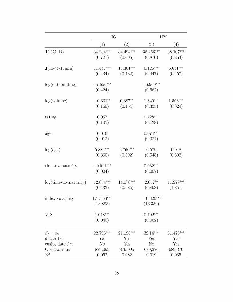
Table 3 provides the results from the regression model in (4). The results show that DC-

DC trades have the lowest spreads and that DC-ID trades have the highest spreads, consistent

14

with our hypothesis. For example, compared with DC-DC spreads (i.e, the base level), the

spreads of DC-ID trades are approximately 34.2 bps higher for IG bonds in column (1) and

38.3 bps higher for HY bonds in column (3), as can be seen from the coefficient estimates

on 1(DC-ID). The spreads of invt>15min trades are also higher by 11.4 bps (IG) and 6.13

bps (HY) than those of DC-DC trades. The difference between the coefficient estimates

on the indicator variables for DC-ID and invt>15min trades are positive and statistically

significant across all columns (see the row for β2−β3). Overall, the results show that DC-DC

spreads are the lowest among all three trade types. The economic magnitudes of differences

in spreads between non-DC-DC trades and DC-DC trades are substantial, given that the

average spread for trades $1 million and above is approximately 35 bps.

In Table 4, we run the regression (4) separately for customer buy and sell trades to

examine whether customers tend to provide liquidity more on buy trades. We find that

the results are consistent with our hypothesis. In IG bond regressions, for example, the

difference in spreads for invt>15min trades and DC-DC trades are 17.2 bps and 6.6 bps

for customer buys and sells, respectively. The difference between the coefficients on DC-

ID and invt>15min trades (i.e., β2 − β3) are also larger for customer buys (25.4 bps) than

for customer sells (17.1 bps). These results show that customer liquidity provision is more

pronounced among customer buy trades.

In Table 5, we run the regression (4) separately for three subsamples based on the number

of customer trades that are $1 million or larger in the past year. For bonds that trade

infrequently, dealers face higher inventory risk and thus compensation to liquidity-providing

customers should be higher. Thus, if the lower spreads on DC-DC trades are driven by having

to compensate the customers that provide liquidity, the difference between DC-DC spreads

and invt>15min spreads should be greater particularly for bonds traded infrequently.

Table 5 provides the regression results. For IG bonds, DC-DC spreads are 32 bps lower

than invt>15min spreads for bonds with 50 or fewer customer trades in the past year, 22 bps

15

lower for bonds with 50 to 100 trades, and 10 bps lower for bonds with more than 100 trades.

Results are similar for HY bonds. These results are consistent with the idea that bid-ask

spreads for DC-DC trades are lower because of customer liquidity provision, especially for

the less active bonds.

Overall, our results show that DC-DC trades have the highest instances of customer

liquidity provision, suggesting that the higher the customer liquidity provision, the more

likely average bid-ask spreads underestimate the cost of demanding liquidity. We examine

this underestimation issue in the next section.

4.2 The Effect of Customer Liquidity Provision on Trading Cost

Measures

In this section, we examine the extent to which various existing bid-ask spread measures in

the literature might underestimate the true cost of immediacy, given substantial amounts of

customer liquidity provision as proxied by DC-DC trades.

Table 2(d) provides summary statistics of various bid-ask spread estimates provided in

Section 3.3—namely, IRC, IRC C, and same-day spread as well as spread1. We find wide

dispersion in average bid-ask spread estimates across the measures. For example, the average

bid-ask spread estimates for IG bonds are 16.7 bps, 17.3 bps, 25.6 bps, and 34.1 bps for

IRC C, IRC, same-day spread, and spread1, respectively.

This dispersion in bid-ask spread estimates across these measures can be explained by the

differences in the fraction of trades used in the calculation of each measure that are DC-DC

trades. IRC C, by construction, is calculated using DC-DC trades almost exclusively and

will understate the cost of demanding immediacy the most. IRC also overweights DC-DC

trades and will understate the cost of liquidity demand. DC-DC trades will also affect same-

day spread estimates, because same-day spread calculation requires both customer buys and

16

sells.

In Table 6, we examine the extent to which DC-DC trades affect the average spread

estimates from these spread measures. The table presents the fractions of DC-DC, DC-ID,

and invt>15min trades for the full sample and the samples that we use to calculate each of

IRC C, IRC, same-day, and spread1 estimates. We find that the IRC C calculation requires

a sample with the highest fraction of DC-DC trades, followed by IRC, same-day spread, and

spread1 calculations. For IG bonds, for example, 82.2%, 61.6%, 21.5%, and 8.2% of the

IRC C, IRC, same-day, and spread1 samples consist of DC-DC trades, respectively. We find

even higher fractions of DC-DC trades in the HY bond samples, suggesting that the effect

of customer liquidity provision in spread estimation is stronger for HY bonds. To the extent

that DC-DC trades are driven by customer liquidity provision, IRC C will understate the

cost of demanding liquidity the most, followed by IRC, same-day spreads, and spread1.10

These results are consistent with the empirical statistics in Table 2(d).

In general, a bid-ask spread measure would understate the cost of immediacy as long as it

puts more weight in short-horizon trades. This poses a conundrum to most spread measures

in the literature. On the one hand, a bid-ask measure should employ more instances of

short-horizon trades, as noise in spread estimates increase with time between consecutive

trades. On the other hand, the measure will more likely underestimate the cost of demanding

immediacy as it places higher weight on short-horizon trades. These opposing effects will

also exist in the weighted-regression-based methods of bid-ask spread estimates in Edwards,

Harris and Piwowar (2007) and Bessembinder et al. (2006). Focusing more on short-horizon

trades will reduce estimation errors, but it will also underestimate the true cost of immediacy

10Because IRC calculations overweight DC-ID trades, one might conclude that this channel will translateinto IRCs being higher. However, this is not necessarily the case because in a DC-ID trade, the customerpays a high spread, of which a large fraction is paid to the second dealer. For example, in a DC-ID trade, ifthe customer pays 30 bps to the first dealer, and if the first dealer passes 20 bps to the second dealer, theaverage customer spread is 30 bps, but the IRC is 10 bps. Table A.2 in Appendix B shows that the profitthat the first dealer makes is similar in DC-DC and DC-ID trades.

17

for customers.

5 Customer Liquidity Provision and Trading Costs Be-

fore and After the Banking Regulations

5.1 Overview of the Recent Banking Regulation Changes

In this section, we briefly discuss the potential impact of the Volcker Rule and capital

regulations on corporate bond liquidity. The Volcker Rule prohibits banks from engaging

in proprietary trading, except when making markets. As Duffie (2012) argues, however, the

Rule may also discourage banks from market-making and providing liquidity. For example,

the Volcker Rule specifies seven quantitative metrics to be reported for certain banks at

the trading desk level, including inventory turnover and inventory aging metrics as well

as customer-facing trade ratios. These requirements may discourage dealers from taking

on inventory and incentivize dealers to offload inventories to customers rather than in the

interdealer market, which is consistent with the rise in customer liquidity provision that we

document in this paper.

Basel III establishes tougher capital rules through increases in the minimum capital

ratio, among many other changes. Stricter capital regulations increase the cost of financing

inventories for dealers. This could lead banks to decrease liquidity provision, especially in

trades that take up large amounts of space in the inventories and are expected to remain

longer.

Since the 2008 financial crisis, corporate bond holdings of banks and broker-dealers have

decreased. Instead, asset managers, especially mutual funds, have increasingly been holding

a larger fraction of outstanding corporate bonds. This has prompted some concerns about

outflow risk (Feroli, Kashyap, Schoenholtz and Shin (2014)). On the other hand, market

18

commentary indicates that these changes have pushed buy-side investors to increasingly be

liquidity providers and price setters in the corporate bond market. For instance, a recent

Bloomberg article documents the increasingly active role that buy-side investors play, and

argues that they have gone from being price takers to price makers.11

5.2 Customer Liquidity Provision Over Time

In this section, we examine the extent to which customer liquidity provision increased in

the post-regulation period using the fraction of DC-DC trades as a measure of customer

liquidity provision. An increase in the fraction of DC-DC trades in the sample will lead to

more severe underestimation in liquidity costs in the corporate bond market.

In Figure 2, we first examine the time series of the fractions of DC-DC and DC-ID trades.

Figure 2 shows that the fractions of DC-DC trades indeed increased in the post-regulation

period, while the fractions of DC-ID trades remained similar or decreased. These plots are

consistent with the notion that there has been a shift from principal trading by dealers to a

pre-arraged, search-and-match trading model and that with this change, increasing fractions

of trades are associated with customer liquidity provision.

While these time series plots hint at regulations playing a role, other changes in the

market may also be driving the results. Thus, we examine how the fractions of DC-DC

trades change differentially for large and small dealers.12 Most large dealers are affiliated

with banks and thus are affected by various bank regulations. In comparison, small dealers

are a mix of bank-affiliated and non-bank dealers and will be less affected by the banking

regulations. In Figure 3, we plot the fractions of DC-DC trades separately for large and

small dealers. Fractions of DC-DC trades increase for large dealers, while there is no distinct

11See https://www.bloomberg.com/news/features/2016-08-15/the-rise-of-the-buy-side12For each month, we first find the top ten dealers by customer trading volume. Using the full sample,

we define large dealers as those that appear in the top ten for a total of ten months or more. Large dealersaccount for 70% or more of trading in trades $1 million and larger, as shown in Table 2(b).

19

pattern for small dealers. These results are consistent with regulations having an effect on

dealers’ inventory holding periods and increasing customer liquidity provision.

To show the above results on DC-DC trades more formally in a regression setting, we

first define the four subperiods: pre-crisis (Jan 2006 to Jun 2007), financial crisis (Jul 2007

to Apr 2009), post-crisis (May 2009 to Jun 2012), and post-regulation (Jul 2012 to Jun 2015)

periods. The choice of July 2012 as the beginning of the post-regulation period is not crucial

for our results. Most of our empirical analyses in this section and Section 5.3 will focus on

comparing the post-regulation period with the pre-crisis and the post-crisis periods.

In Table 7, we regress the daily fractions of DC-DC trades on dummy variables for each

subperiod:

Aggregate level : yt = α +4∑

l=2

βl1(t ∈ Tl) + εt (5)

Dealer group level : ym,t = α1 + α21(small)m +4∑

l=2

1(large)mβlarge,l1(t ∈ Tl)

+4∑

l=2

1(small)mβsmall,l1(t ∈ Tl) + εm,t (6)

Individual dealer level : yj,t =∑j

Dj +4∑

l=2

βl1(t ∈ Tl) + εj,t. (7)

The aggregate level fraction of DC-DC trades, yt, is calculated as the daily volume-weighted

average of DC-DC fractions across bonds and dealers. The dealer group level fraction of

DC-DC trades, ym,t, is the average fraction of DC-DC trades calculated separately for large

and small dealers. The indicator variables, 1(large)m and 1(small)m, are for large and

small dealer groups, respectively. The individual dealer fraction of DC-DC trades, yj,t, is the

fraction of DC-DC trades for dealer j on day t. Tl (l = 1, . . . , 4) are the four subperiods (pre-

crisis, financial crisis, post-crisis, post-regulation). We include the VIX and bond market

volatility as control variables. For the individual dealer regression, we use only the 15 largest

20

dealers and run both OLS and median regressions. The median regression is used to rule

out the possibility that the results are driven by one or a few large dealers.13

Table 7 presents the regression results. Consistent with Figure 2, the results indicate that

customers provide more liquidity and that dealers take on less risk in the post-regulation

period compared with the pre-crisis and the post-crisis periods. In column (5) for HY bonds,

for example, the coefficient on the post-regulation dummy is 7.5% and statistically significant

at the 1% level, showing that the fraction of DC-DC trades are 7.5 percentage points higher

in the post-regulation period compared with the pre-crisis levels, which forms the base level.

Also in column (5), the fraction of DC-DC trades post-regulation is also higher than the

post-crisis level as well, as the difference between the coefficients on the post-regulation

dummy and the post-crisis dummy (row β4 − β3 near the bottom) is 4.1% and statistically

significant at the 1% level. We find similar results for IG bonds in column (1).

Table 7 also shows that these increases in customer liquidity provision and decreases in

dealer risk taking are driven mainly by large dealers, consistent with regulations affecting

bank-affiliated dealers. In the dealer group level regression for HY bonds in column (6),

for instance, the coefficient estimate on the interaction between the large dealer dummy

and post-regulation dummy is 8.4% and highly statistically significant, showing that large

dealers increase the fraction of DC-DC trades in the post-regulation period compared to the

pre-crisis period. Furthermore, the difference between the coefficient on large × post-reg and

large × post-crisis is statistically significant at the 1% level (see row βlarge,4 − βlarge,3 near

the bottom), thus the faction of DC-DC trades in the post-regulation period is even higher

than the post-crisis level for large dealers. In contrast, during the same period the small

dealers decrease the fraction of DC-DC trades by 4.3%, as can be seen from the difference

between the coefficients on small × post-reg and small × post-crisis also reported in row

13Given that some of the large dealers have a substantial fraction of the total trading volume, the increasein DC-DC trades can be due to one large dealer increasing the amounts of DC-DC trades substantially.

21

βsmall,4−βsmall,3. For IG bonds, both large and small dealers increase the fraction of DC-DC

trades for investment grade bonds, as can be seen from the difference test on βlarge,4−βlarge,3

and βsmall,4 − βsmall,3 reported in column (2). We also find that results for individual dealer

level regressions in columns (3), (4), (7), and (8) are similar to that of the aggregate level

regressions, and thus, these results are not driven by outliers.

Overall, the results in this section show that customer liquidity provision increased in

the post-regulation period compared with the pre-crisis and the post-crisis periods. This

increase is driven mostly by large dealers, which is consistent with bank regulations having

had an impact.

5.3 Trading Costs Over Time

Our results thus far show that customer liquidity provision, as measured by the fractions of

DC-DC trades, has increased in the post-regulation period. Thus, the usual bid-ask spread

measures in the literature that are calculated using liquidity-providing customer trades would

underestimate what liquidity-demanding customers would pay, particularly during the post-

regulation period. In this section, we examine how severe underestimation in bid-ask spreads

is during the post-regulation period.

In Table 8, we examine how this underestimation in the common bid-ask spread measures

influences our inference on the liquidity of corporate bonds in the post-regulation period.

We employ the previous three bid-ask spread measures, i.e., IRC C, IRC, and same-day

spreads as test cases. To the extent that DC-DC trades are used in the calculation of these

measures, they will understate the true cost of immediacy. As a benchmark case with respect

to these three measures, we also calculate bid-ask spreads based on the spread1 measure but

using invt>15min trades only (“invt>15min spreads”). As invt>15min trades are largely

trades where dealers provide immediacy to customers, focusing only on the invt>15min

22

trades would alleviate the underestimation issue.14 We compare post-regulation transaction

costs across these four cases (i.e., the three common measures and the benchmark spread1

measure using invt>15min only).

We then estimate the following model for each of the four measures:

spreadi,t = α +4∑

l=2

βl1(t ∈ Tl) + εi,t (8)

where spreadi,t is the trading cost measure for bond i on day t. Tl (l = 1, . . . , 4) are the

subperiod dummies, and T1 is the omitted base level due to multicollinearity. We control

for bond characteristics such as outstanding amount, ratings, age, and time-to-maturity and

market-level variables such as the bond index volatility and VIX, as well as the average

customer trade size for bond i on day t. We also perform a statistical test for β4 − β3, the

difference between the coefficient for post-regulation dummy and the coefficient for post-crisis

dummy.

Table 8(a) presents the estimation results for investment grade bonds. As the coefficient

estimate on post-regulation in column (4) indicates, the invt>15min spreads are 12.7 bps

higher in the post-regulation period compared with the pre-crisis period (the base level).

This difference is economically significant as the average of spread1 is approximately 35 bps

for the full sample, and around 25 bps for the non-crisis periods. In contrast, using the other

trading cost measures in columns (1) through (3) underestimates this increase in trading

costs during the post-regulation period. In column (1) when IRC C is used, for example,

the estimated difference in trading cost between the post-regulation period and pre-crisis

period is 0.9 bps (see the coefficient on post-regulation). Similarly, the coefficient estimates

on post-regulation are 2.4 bps and 6.5 bps for IRC (column 2) and same-day spreads (column

3), respectively. Hence, using IRC C underestimates the post-regulation increase in bid-ask

14We also exclude DC-ID matched trades to focus on trades were dealers provided immediacy.

23

spreads the most, followed by IRC and same-day spreads. Looking at the differences between

the post-crisis and the post-regulation periods (i.e., row β4 − β3 at the bottom of the table)

yield similar results; IRC C and IRC would indicate that trading costs have not changed

between the two periods, while invt>15min spreads show a 3.9 bps increase.

We find qualitatively similar results for HY bonds in Panel (b) and also when we use

regression specifications without bond-level controls in Panels (c) and (d). Overall, these

results also show why using some of these other measures might result in the conclusion

that trading costs have not increased post-regulation. For instance, Panel (d) indicates

that trading costs for high-yield bonds are lower in the post-regulation period compared to

the pre-crisis period if we use IRC C, IRC, or same-day spreads, as can be seen from the

coefficient estimates on post-regulation. In column (4), however, the same coefficient estimate

shows that invt>15min spreads are 3.6 bps higher in the post-regulation period.

As a robustness check, in Table 9 we run a difference-in-differences-style test to examine

whether differences in the coefficient estimates across samples are statistically signfiicant.

Specifically, we compare each of the three trading cost measures, y, with the benchmark

measure, which is spread1 estimated using invt>15min only. We first define the difference

between the trading cost measure and the benchmark, diffi,t, as:

diffi,t = yi,t − (invt>15min spread)i,t (9)

where yi,t is either IRC C, IRC, or same-day spread for bond i on day t. Then, we run the

difference-in-difference regression as

diffi,t = α +4∑

l=2

βl1(t ∈ Tl)εi,t. (10)

Note that diffi,t can be calculated only for bond-days where both y and invt>15min spread

exist, and thus this regression analysis does not necessarily test the difference in estimates

24

between y and invt>15min spreads from (8).

Table 9 presents the regression in (10). Consistent with our prediction, IRC C under-

estimates the change in trading costs the most, followed by IRC and same-day spreads. In

column (4), for example, the coefficient on post-regulation is -6.2 bps and is statistically

significant at 1% level, indicating that the bid-ask spread estimates using IRC C is lower

than the benchmark spread calculated using invt>15min trades. We find similar results for

the other spread measures reported in columns (5) and (6). The results provided in Table

Table 9 confirm those reported in Table 8.

There are two main takeaways from this section. First, trading costs for liquidity-

demanding customers, as measured by invt>15min spreads, have increased by 10–13 bps

in the post-regulation period compared with the pre-crisis period and 4–7 bps compared

with the post-crisis period. Given that average bid-ask spreads during non-crisis times are

around 25 bps, these increases are substantial. Moreover, since invt>15min trades do con-

tain trades where customers are providing liquidity, these 10–13 bps increases are likely

underestimates as well.

Second, some of liquidity measures often used in the literature might understate this

increase in costs for demanding liquidity. Using IRC and same-day spreads, for instance,

Anderson and Stulz (2017), Trebbi and Xiao (2017), and Adrian, Fleming, Shachar and

Vogt (2017) conclude that price measures of liquidity has not worsened. Our results help

explain why bid-ask spread estimates reported in the previous studies did not increase in the

post-regulation period despite reduction in the inventory capacity of financial intermediaries.

6 Conclusion

We show that substantial amounts of liquidity are provided by the non-dealer sector and that

this provision of liquidity by non-dealers causes the average bid-ask spreads to underestimate

25

the cost of immediacy paid by liquidity-demanding customers. Decreases in dealers’ willing-

ness or ability to provide inventories have pushed more liquidity provision to the non-dealer

sector, which in turn has made the bias more severe. We show that these mechanisms lead

to an underestimation of the impact of regulations on liquidity, and once we reduce this bias,

measured costs of demanding immediacy in the U.S. corporate bond markets have increased

post-regulation. This increase in transaction costs are consistent with the Volcker Rule and

more stringent capital regulations having affected liquidity in the OTC markets.

Overall, the net effect of decreased dealer liquidity provision to customers may be am-

biguous. Some buy-side investors who have enough liquidity and the expertise to provide

liquidity may benefit from the reduced capabilities of the dealer sector in providing liquid-

ity during the post-regulation period. For other customers that generally demand liquidity

only, both the cost of immediacy and the average waiting time have increased in the post-

regulation period. Also, the increased liquidity provision by the non-dealer sector may be

unhealthy for the stability of financial markets. Given that many non-dealers are likely buy-

side participants subject to potential liquidity shocks from fund outflows, these shocks may

have feedback effects. These potential negative consequences should be weighed against the

potential positive impact that regulations have had on curbing systemic risk. We believe

that it would be an interesting future research to examine such welfare consequences of these

regulations.

26

References

Adrian, T., Boyarchenko, N. and Shachar, O. (2017), ‘Dealer balance sheets and bond liq-

uidity provision’, Journal of Monetary Economics 89, 92–109.

Adrian, T., Fleming, M. J., Shachar, O. and Vogt, E. (2017), ‘Market liquidity after the

financial crisis’, Annual Review of Financial Economics 9(1).

Anderson, M. and Stulz, R. M. (2017), ‘Is post-crisis bond liquidity lower?’, NBER Working

Paper .

Bao, J., O’Hara, M. and Zhou, X. A. (2017), ‘The Volcker rule and market-making in times

of stress’, forthcoming, Journal of Financial Economics .

Bessembinder, H., Jacobsen, S. E., Maxwell, W. F. and Venkataraman, K. (2017), ‘Capital

commitment and illiquidity in corporate bonds’, forthcoming, Journal of Finance .

Bessembinder, H., Maxwell, W. and Venkataraman, K. (2006), ‘Market transparency, liquid-

ity externalities, and institutional trading costs in corporate bonds’, Journal of Financial

Economics 82(2), 251–288.

BlackRock (2015), ‘Addressing market liquidity’, BlackRock Viewpoint July.

BofA Merrill Lynch (n.d.), ‘BofA Merrill Lynch Bond Indices’, retrieved from FRED, Federal

Reserve Bank of St. Louis, https://fred.stlouisfed.org/.

Chakravarty, S. and Sarkar, A. (2003), ‘Trading costs in three us bond markets’, The Journal

of Fixed Income 13(1), 39–48.

Cimon, D. A. and Garriott, C. (2016), ‘Banking regulation and market making’, Bank of

Canada Working Paper .

27

Dick-Nielsen, J. and Rossi, M. (2016), ‘The cost of immediacy for corporate bonds’, Working

Paper .

Duffie, D. (2012), ‘Market making under the proposed volcker rule’, Rock Center for Corpo-

rate Governance at Stanford University Working Paper (106).

Edwards, A. K., Harris, L. E. and Piwowar, M. S. (2007), ‘Corporate bond market transac-

tion costs and transparency’, The Journal of Finance 62(3), 1421–1451.

Feldhutter, P. (2012), ‘The same bond at different prices: identifying search frictions and

selling pressures’, Review of Financial Studies 25(4), 1155–1206.

Feroli, M., Kashyap, A. K., Schoenholtz, K. L. and Shin, H. S. (2014), ‘Market tantrums

and monetary policy’, Paper for the U.S. Monetary Policy Forum, New York .

Financial Industry Regulatory Authority (n.d.), ‘Bond Trade Dissemination System (BTDS)

and Trade Reporting and Compliance Engine (TRACE)’, http://www.finra.org/

Industry/Compliance/MarketTransparency/TRACE/index.htm.

Goldstein, M. A. and Hotchkiss, E. S. (2017), ‘Providing liquidity in an illiquid market:

Dealer behavior in U.S. corporate bonds’, Working Paper .

Goldstein, M. A., Hotchkiss, E. S. and Sirri, E. R. (2007), ‘Transparency and liquidity: A

controlled experiment on corporate bonds’, Review of Financial Studies 20(2), 235–273.

Harris, L. (2015), ‘Transaction costs, trade throughs, and riskless principal trading in cor-

porate bond markets’, Working Paper .

Hong, G. and Warga, A. (2000), ‘An empirical study of bond market transactions’, Financial

Analysts Journal 56(2), 32–46.

28

Mergent, Inc. (n.d.), ‘Mergent Corporate FISD Daily Feed (FITF)’, http://www.

ftserussell.com/financial-data/fixed-income-data.

Schultz, P. (2017), ‘Inventory management by corporate bond dealers’, Working Paper .

Trebbi, F. and Xiao, K. (2017), ‘Regulation and market liquidity’, Management Science,

forthcoming .

Uslu, S. (2016), ‘Pricing and liquidity in decentralized asset markets’, Working Paper .

Zitzewitz, E. (2010), ‘Paired corporate bond trades’, Working Paper .

29

Figure 1: Time-Series Plot of Fraction of Trades with AffiliatesThis figure plots the fraction of trades between dealers and their non-FINRA affiliates withrespect to total customer trades. Appendix A explains the algorithm used to identify affiliatetrades.

0.000

0.025

0.050

0.075

2006 2008 2010 2012 2014

date

Fra

ctio

n of

vol

ume

HY IG

30

Figure 2: Time Series Plot of the Fraction of DC-DC and DC-ID TradesThis figure plots the monthly fraction of customer trades that are DC-DC (red solid line)and DC-ID trades (blue dotted line) with respect to total customer trade volumes over thesample period. Panel A plots IG bond trades, and Panel B plots HY bond trades.

0.05

0.10

0.15

0.20

2006 2008 2010 2012 2014

date

Fra

ctio

n of

vol

ume

A. Investment grade

0.1

0.2

0.3

2006 2008 2010 2012 2014

date

Fra

ctio

n of

vol

ume

B. High yield

DC−DC DC−ID

31

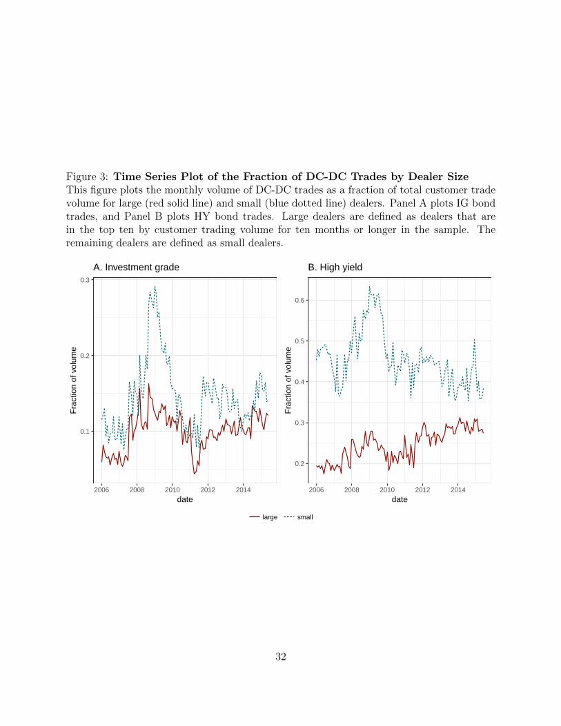
Figure 3: Time Series Plot of the Fraction of DC-DC Trades by Dealer SizeThis figure plots the monthly volume of DC-DC trades as a fraction of total customer tradevolume for large (red solid line) and small (blue dotted line) dealers. Panel A plots IG bondtrades, and Panel B plots HY bond trades. Large dealers are defined as dealers that arein the top ten by customer trading volume for ten months or longer in the sample. Theremaining dealers are defined as small dealers.

0.1

0.2

0.3

2006 2008 2010 2012 2014

date

Fra

ctio

n of

vol

ume

A. Investment grade

0.2

0.3

0.4

0.5

0.6

2006 2008 2010 2012 2014

date

Fra

ctio

n of

vol

ume

B. High yield

large small

32

Figure 4: Time Series Plot of Various Trading Cost MeasuresThis figure plots the monthly time series of IRC C (red solid line), same-day spreads (greendotted line), and spread1 measured using invt>15min trades (blue dashed line) for IG (PanelA) and HY (Panel B) bonds.

25

50

75

100

2006 2008 2010 2012 2014

date

spre

ad (

bp)

A. Investment grade

25

50

75

100

2006 2008 2010 2012 2014

date

spre

ad (

bp)

B. High yield

IRC_C same−day spread invt>15min spread

33

Table 1: An Example of Matching Customer Trades

Panel A: Sample (Ficticious) Trading Data

trade num time trade type dealer buy/dealer sell quantity

1 10:00:00 AM DC S 2002 10:00:05 AM DC B 2003 11:20:07 AM DC B 4004 11:50:00 AM DC B 5005 12:02:03 PM ID S 3506 12:30:00 PM DC S 1007 1:00:00 PM DC B 5508 1:00:03 PM DC S 1009 1:00:05 PM ID S 400

Panel B: Trade Matching and Holding Period Calculation

trade num other side holding period volume short holding short type overnight

1 2 00:00:05 200 1 DC-DC 02 1 00:00:05 200 1 DC-DC 03 NA NA 400 0 14 5 00:12:03 350 1 DC-ID 04 6 00:40:00 100 0 04 NA NA 50 0 16 4 00:40:00 100 0 07 8 00:00:03 100 1 DC-DC 07 9 00:00:05 400 1 DC-ID 07 NA NA 50 0 18 7 00:00:03 100 1 DC-DC 0

Panel C: Trade Classification

trade num vwavg(short) vwavg(DC-DC | short) vwavg(DC-ID | short) trade type

1 1 1 0 DC-DC2 1 1 0 DC-DC3 0 invt>15min4 0.7 0 1 DC-ID6 0 0 0 invt>15min7 0.91 0.2 0.8 DC-ID8 1 1 0 DC-DC

34

Table 2: Summary StatisticsThis table reports summary statistics on corporate bond trades and transaction cost esti-mates. Panel (a) reports the fractions of overnight, DC-DC, DC-ID, and invt>15min tradesby rating (IG vs. HY) and trade size ($100K or less, $100K to $1 million, $1 million andlarger) groups. We report the fractions of trades in columns 3 through 6, trade volumein billion USD in column 7, and trade count (the number of trades) in column 8. Pan-els (b) and (c) reports the same statistics as Panel (a) but by rating (IG vs. HY) anddealer size groups in Panel (b) and by rating (IG vs. HY) and trade count groups in Panel(c). Panel (d) reports the averages of trading costs estimated using IRC C, IRC, same-day spread, and spread1 methods. We also report average spread1 for DC-DC, DC-ID,and invt>15min trades separately. Column #(bond-days) reports the number of bond-dayobservations. Panel (e) reports the fraction of customer trades with negative spread1 forDC-DC, DC-ID, and invt>15 min trades across rating groups (IG and HY) and trade di-rections (customer buy and sell). In Panel (a), we use all customer trades, while Panels (b)through (e) use customer trades $1 million and larger only. The sample period is from 2006to 2015.

(a) Fractions of Customer Trades by Rating and Trade Size

rating trade size overnight DC-DC DC-ID invt>15min volume trade count

IG ≤100K 49.25% 3.31% 27.25% 69.44% 284 9,697,291IG 100K-1mil 71.16% 4.60% 10.43% 84.97% 961 2,747,612IG ≥ 1mil 66.06% 9.60% 5.21% 85.19% 10,576 2,233,523HY ≤100K 47.01% 3.65% 25.35% 71.00% 98 3,354,601HY 100K-1mil 60.75% 11.33% 9.26% 79.41% 394 1,041,394HY ≥ 1mil 49.04% 23.89% 4.03% 72.08% 5,835 1,707,177

(b) Fractions of Customer Trades by Rating and Dealer Size

rating dealer size overnight DC-DC DC-ID invt>15min volume trade count

IG large 71.42% 8.20% 2.69% 89.11% 8,104 1,555,775IG small 53.75% 12.81% 10.99% 76.20% 2,472 677,748HY large 55.43% 19.40% 2.63% 77.97% 4,893 1,381,711HY small 21.92% 42.96% 9.97% 47.06% 943 325,466

35

(c) Fractions of Customer Trades by Rating and Trade Count Per Year

rating # trade/year overnight DC-DC DC-ID invt>15min volume trade count

IG (0,20] 59.66% 14.41% 6.41% 79.19% 748 182,018IG (20,50] 65.77% 10.85% 5.27% 83.88% 1,676 392,599IG (50,100] 68.13% 9.35% 5.17% 85.47% 2,398 527,197IG (100,Inf] 66.23% 8.50% 5.01% 86.49% 5,753 1,131,709HY (0,20] 39.57% 38.47% 4.54% 56.99% 166 42,834HY (20,50] 42.96% 34.44% 3.41% 62.15% 495 142,783HY (50,100] 47.92% 28.71% 3.41% 67.88% 920 280,064HY (100,Inf] 50.32% 21.09% 4.22% 74.69% 4,254 1,241,496

(d) Average Bid-Ask Spreads Across Various Estimation Methods

IG HY

average spread (bps) #(bond-days) average spread (bps) #(bond-days)

IRC C 16.65 84,374 25.60 107,866IRC 17.25 152,243 25.68 130,264same day 25.59 344,645 28.59 333,690spread1 34.14 464,825 37.80 248,368

DC-DC 16.26 34,043 25.80 52,222DC-ID 58.56 54,097 68.78 37,158invt>15min 32.97 430,008 36.06 224,532

(e) Fractions of Negative Spread Trades

DC-DC DC-ID invt>15min

ratingIG 41.59% 13.93% 31.17%HY 37.26% 16.19% 32.75%

trade directioncustomer buy 43.08% 14.63% 34.45%customer sell 34.30% 15.27% 28.99%

36

Table 3: Regressions of Bid-Ask Spreads on Customer Trade TypesThis table presents the results from the following panel regression for IG (columns 1 and 2)and HY bonds (columns 3 and 4)

spread1 i,j,t,k = α + β21(DC-ID)k + β31(invt>15min)k + εi,j,t,k

where spread1 i,j,t,k is the spread1 for customer trade k of bond i on day t with dealer j.1(DC-ID)k and 1(invt>15min)k are dummy variables for DC-ID and invt>15min trades,respectively. We omit the dummy variable for DC-DC trades. Control variables are logamount outstanding of bond i, log trading volume, bond rating, both age and log age of thebond, log time-to-maturity of the bond, volatility of bond index returns, and the VIX. Wealso include bond and time fixed effects as well as dealer fixed effects. Row β2−β3 reports thecoefficient difference between β2 and β3 and its statistical significance. The sample period isfrom 2006 to 2015, and we restrict the sample to trades over $1 million. Standard errors aredouble clustered by bond and date. *, **, and *** denote statistical significant at the 10%,5%, and 1% levels, respectively.

37

IG HY

(1) (2) (3) (4)

1(DC-ID) 34.234∗∗∗ 34.494∗∗∗ 38.266∗∗∗ 38.107∗∗∗

(0.721) (0.695) (0.876) (0.863)

1(invt>15min) 11.441∗∗∗ 13.301∗∗∗ 6.126∗∗∗ 6.631∗∗∗

(0.434) (0.432) (0.447) (0.457)

log(outstanding) −7.550∗∗∗ −6.960∗∗∗

(0.424) (0.562)

log(volume) −0.331∗∗ 0.387∗∗ 1.340∗∗∗ 1.503∗∗∗

(0.160) (0.154) (0.335) (0.329)

rating 0.057 0.728∗∗∗

(0.105) (0.138)

age 0.016 0.074∗∗∗

(0.012) (0.024)

log(age) 5.884∗∗∗ 6.766∗∗∗ 0.579 0.948(0.360) (0.392) (0.545) (0.592)

time-to-maturity −0.011∗∗∗ 0.032∗∗∗

(0.004) (0.007)

log(time-to-maturity) 12.854∗∗∗ 14.078∗∗∗ 2.052∗∗ 11.979∗∗∗

(0.433) (0.535) (0.893) (1.357)

index volatility 171.356∗∗∗ 110.326∗∗∗

(18.888) (16.350)

VIX 1.048∗∗∗ 0.702∗∗∗

(0.040) (0.062)

β2 − β3 22.793∗∗∗ 21.193∗∗∗ 32.14∗∗∗ 31.476∗∗∗

dealer f.e. Yes Yes Yes Yescusip, date f.e. No Yes No YesObservations 879,095 879,095 689,376 689,376R2 0.052 0.082 0.019 0.035

38

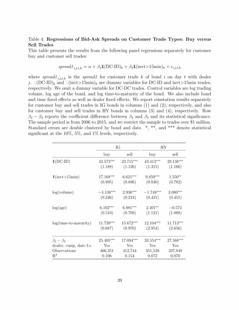
Table 4: Regressions of Bid-Ask Spreads on Customer Trade Types: Buy versusSell TradesThis table presents the results from the following panel regressions separately for customerbuy and customer sell trades:

spread1 i,j,t,k = α + β21(DC-ID)k + β31(invt>15min)k + εi,j,t,k

where spread1 i,j,t,k is the spread1 for customer trade k of bond i on day t with dealerj. 1(DC-ID)k and 1(invt>15min)k are dummy variables for DC-ID and invt>15min trades,respectively. We omit a dummy variable for DC-DC trades. Control variables are log tradingvolume, log age of the bond, and log time-to-maturity of the bond. We also include bondand time fixed effects as well as dealer fixed effects. We report esimtation results separatelyfor customer buy and sell trades in IG bonds in columns (1) and (2), respectively, and alsofor customer buy and sell trades in HY bonds in columns (3) and (4), respectively. Rowβ2 − β3 reports the coefficient difference between β2 and β3 and its statistical significance.The sample period is from 2006 to 2015, and we restrict the sample to trades over $1 million.Standard errors are double clustered by bond and date. *, **, and *** denote statisticalsignificant at the 10%, 5%, and 1% levels, respectively.

IG HY

buy sell buy sell

1(DC-ID) 42.573∗∗∗ 23.715∗∗∗ 43.413∗∗∗ 29.138∗∗∗

(1.188) (1.126) (1.315) (1.166)

1(invt>15min) 17.168∗∗∗ 6.621∗∗∗ 9.859∗∗∗ 1.550∗∗

(0.895) (0.896) (0.830) (0.782)

log(volume) −4.138∗∗∗ 2.936∗∗∗ −1.748∗∗∗ 3.080∗∗∗

(0.246) (0.218) (0.431) (0.451)

log(age) 6.102∗∗∗ 6.881∗∗∗ 2.401∗∗ −0.574(0.510) (0.708) (1.131) (1.088)

log(time-to-maturity) 11.739∗∗∗ 15.672∗∗∗ 12.104∗∗∗ 11.713∗∗∗

(0.687) (0.970) (2.954) (2.656)

β2 − β3 25.405∗∗∗ 17.094∗∗∗ 33.554∗∗∗ 27.588∗∗∗

dealer, cusip, date f.e. Yes Yes Yes YesObservations 466,351 412,744 351,528 337,848R2 0.106 0.154 0.072 0.070

39

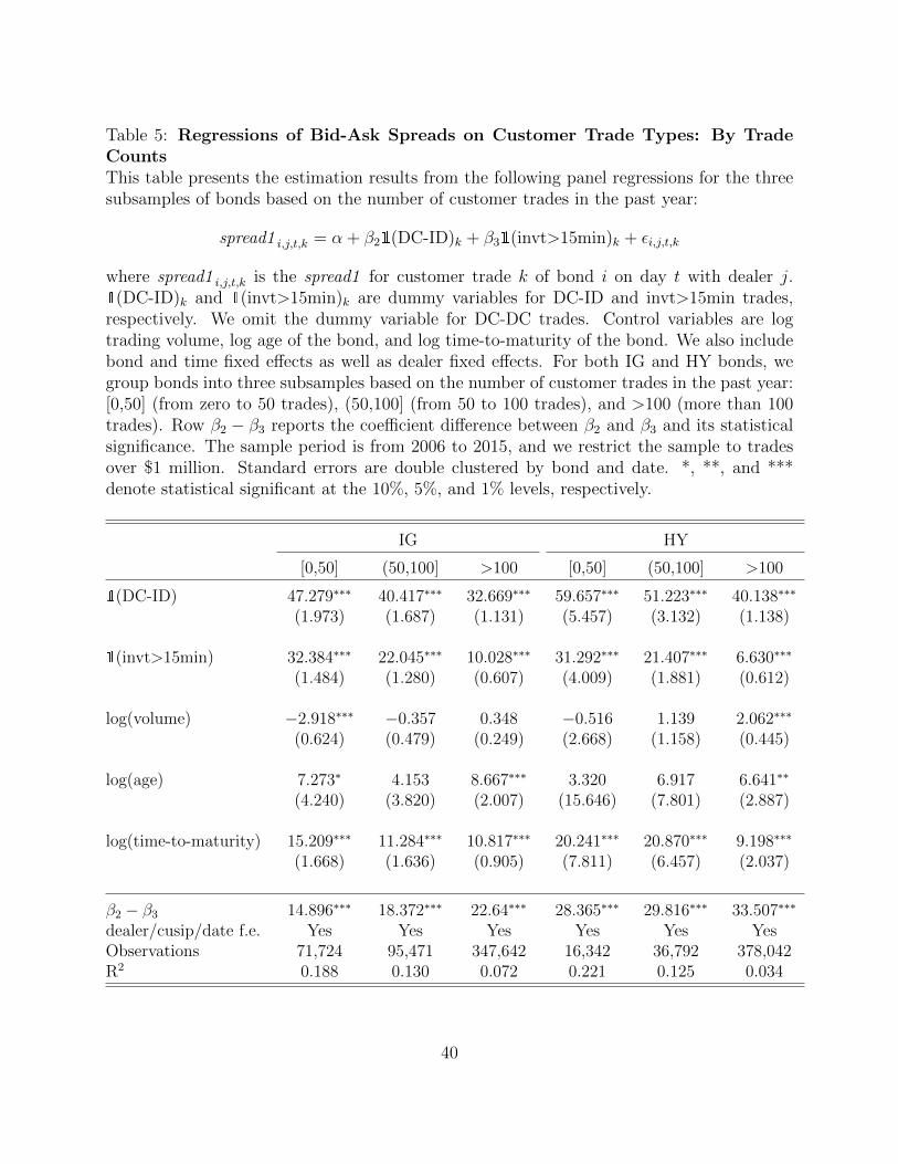
Table 5: Regressions of Bid-Ask Spreads on Customer Trade Types: By TradeCountsThis table presents the estimation results from the following panel regressions for the threesubsamples of bonds based on the number of customer trades in the past year:

spread1 i,j,t,k = α + β21(DC-ID)k + β31(invt>15min)k + εi,j,t,k

where spread1 i,j,t,k is the spread1 for customer trade k of bond i on day t with dealer j.1(DC-ID)k and 1(invt>15min)k are dummy variables for DC-ID and invt>15min trades,respectively. We omit the dummy variable for DC-DC trades. Control variables are logtrading volume, log age of the bond, and log time-to-maturity of the bond. We also includebond and time fixed effects as well as dealer fixed effects. For both IG and HY bonds, wegroup bonds into three subsamples based on the number of customer trades in the past year:[0,50] (from zero to 50 trades), (50,100] (from 50 to 100 trades), and >100 (more than 100trades). Row β2 − β3 reports the coefficient difference between β2 and β3 and its statisticalsignificance. The sample period is from 2006 to 2015, and we restrict the sample to tradesover $1 million. Standard errors are double clustered by bond and date. *, **, and ***denote statistical significant at the 10%, 5%, and 1% levels, respectively.

IG HY

[0,50] (50,100] >100 [0,50] (50,100] >100

1(DC-ID) 47.279∗∗∗ 40.417∗∗∗ 32.669∗∗∗ 59.657∗∗∗ 51.223∗∗∗ 40.138∗∗∗

(1.973) (1.687) (1.131) (5.457) (3.132) (1.138)

1(invt>15min) 32.384∗∗∗ 22.045∗∗∗ 10.028∗∗∗ 31.292∗∗∗ 21.407∗∗∗ 6.630∗∗∗

(1.484) (1.280) (0.607) (4.009) (1.881) (0.612)

log(volume) −2.918∗∗∗ −0.357 0.348 −0.516 1.139 2.062∗∗∗

(0.624) (0.479) (0.249) (2.668) (1.158) (0.445)

log(age) 7.273∗ 4.153 8.667∗∗∗ 3.320 6.917 6.641∗∗

(4.240) (3.820) (2.007) (15.646) (7.801) (2.887)

log(time-to-maturity) 15.209∗∗∗ 11.284∗∗∗ 10.817∗∗∗ 20.241∗∗∗ 20.870∗∗∗ 9.198∗∗∗

(1.668) (1.636) (0.905) (7.811) (6.457) (2.037)

β2 − β3 14.896∗∗∗ 18.372∗∗∗ 22.64∗∗∗ 28.365∗∗∗ 29.816∗∗∗ 33.507∗∗∗

dealer/cusip/date f.e. Yes Yes Yes Yes Yes YesObservations 71,724 95,471 347,642 16,342 36,792 378,042R2 0.188 0.130 0.072 0.221 0.125 0.034

40

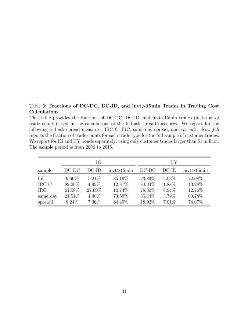
Table 6: Fractions of DC-DC, DC-ID, and invt>15min Trades in Trading CostCalculationsThis table provides the fractions of DC-DC, DC-ID, and invt>15min trades (in terms oftrade counts) used in the calculations of the bid-ask spread measures. We report for thefollowing bid-ask spread measures: IRC C, IRC, same-day spread, and spread1. Row fullreports the fraction of trade counts for each trade type for the full sample of customer trades.We report for IG and HY bonds separately, using only customer trades larger than $1 million.The sample period is from 2006 to 2015.

IG HY

sample DC-DC DC-ID invt>15min DC-DC DC-ID invt>15min

full 9.60% 5.21% 85.19% 23.89% 4.03% 72.08%IRC C 82.20% 4.99% 12.81% 84.84% 1.88% 13.28%IRC 61.58% 27.69% 10.74% 78.30% 8.94% 12.76%same day 21.51% 4.90% 73.59% 35.44% 3.79% 60.78%spread1 8.24% 7.36% 84.40% 18.92% 7.01% 74.07%

41

Table 7: Regression of the Fraction of DC-DC trades on Pre- and Post-RegulationDummy VariablesThis table provides the estimation results from the following regressions at the aggregate,dealer group, and individual dealer levels:

Aggregate level : yt = α +4∑

l=2

βl1(t ∈ Tl) + εt

Dealer group level : ym,t = α1 + α21(small)m +4∑

l=2

1(large)mβlarge,l1(t ∈ Tl)

+4∑

l=2

1(small)mβsmall,l1(t ∈ Tl) + εm,t

Individual dealer level : yj,t =∑j

Dj +4∑

l=2

βl1(t ∈ Tl) + εj,t

where the dependent variables, yt, ym,t, and yj,t, are the fractions of daily DC-DC trade vol-umes at the aggregate, dealer group, and individual dealer levels, respectively. The aggregatelevel fraction of DC-DC trades, yt, is calculated as the daily volume-weighted average of DC-DC fractions across bonds and dealers. Tl (l = 1, . . . , 4) are the four subperiods (pre-crisis,financial crisis, post-crisis, post-regulation) and the dummy variables, 1(t ∈ Tl), indicate thefour subperiods. 1(T1) is the omitted dummy, and thus, forms the base level. We report theaggregate (agg), dealer group (group), and individual dealer (ind) level regressions for IGbonds in columns (1), (2), and (3), respectively. Column (4) (ind med) reports the medianregression of IG bonds at the individual dealer level. Columns (5) through (8) report thesame set of regressions for HY bonds. The dealer group level fraction of DC-DC trades,ym,t, is the average fraction of DC-DC trades calculated separately for large and small deal-ers, where the large dealer group consists of 15 largest dealers and the small dealer groupconsists of the rest. The indicator variables, 1(large)m and 1(small)m, are for large andsmall dealer groups, respectively. The individual dealer fraction of DC-DC trades, yj,t, isthe fraction of DC-DC trades for dealer j on day t. We include the VIX and bond marketvolatility as control variables. We also report the differences in coefficients and their statis-tical significance in the five rows at the bottom of the table. We use Newey-West standarderrors with 20 lags for the aggregate level regression and use standard errors clustered bydate for the dealer group and individual dealer regressions. We calculate standard errors forthe individual dealer level median regression based on 2,000 bootstraps. The sample periodis from 2006 to 2015. *, **, and *** denote statistical significant at the 10%, 5%, and 1%levels, respectively.

42

IG HY

agg group ind OLS ind med agg group ind OLS ind med(1) (2) (3) (4) (5) (6) (7) (8)

crisis 0.032∗∗∗ 0.059∗∗∗ 0.031∗∗∗ 0.023∗∗∗ 0.032∗∗∗ 0.035∗∗∗

(0.007) (0.004) (0.003) (0.007) (0.004) (0.004)

post-crisis 0.019∗∗∗ 0.038∗∗∗ 0.009∗∗∗ 0.034∗∗∗ 0.023∗∗∗ 0.030∗∗∗

(0.005) (0.002) (0.002) (0.007) (0.003) (0.003)

post-regulation 0.042∗∗∗ 0.070∗∗∗ 0.031∗∗∗ 0.075∗∗∗ 0.057∗∗∗ 0.074∗∗∗

(0.003) (0.002) (0.002) (0.004) (0.003) (0.003)

index volatility 0.334∗∗ 0.332∗∗∗ 0.219∗∗∗ 0.096∗ 0.049 0.024 −0.007 −0.049(0.133) (0.075) (0.066) (0.057) (0.127) (0.086) (0.058) (0.066)

VIX 0.001∗∗∗ 0.002∗∗∗ 0.001∗∗∗ 0.001∗∗∗ 0.002∗∗∗ 0.002∗∗∗ 0.001∗∗∗ 0.001∗∗∗

(0.0002) (0.0002) (0.0001) (0.0001) (0.001) (0.0003) (0.0002) (0.0002)

small 0.033∗∗∗ 0.251∗∗∗

(0.003) (0.005)

large × crisis 0.008∗∗ 0.005(0.004) (0.004)

small × crisis 0.053∗∗∗ 0.036∗∗∗

(0.006) (0.008)

large × post-crisis 0.008∗∗∗ 0.020∗∗∗

(0.003) (0.004)

small × post-crisis 0.020∗∗∗ −0.0005(0.004) (0.007)

large × post-reg 0.039∗∗∗ 0.084∗∗∗

(0.002) (0.003)

small × post-reg 0.034∗∗∗ −0.044∗∗∗

(0.004) (0.006)

Constant 0.044∗∗∗ 0.031∗∗∗ 0.007∗∗ 0.016∗∗∗ 0.200∗∗∗ 0.161∗∗∗ 0.178∗∗∗ 0.157∗∗∗

(0.005) (0.003) (0.003) (0.003) (0.007) (0.004) (0.004) (0.004)

dealer f.e. Yes Yes Yes Yes

β4 − β3 0.022∗∗∗ 0.032∗∗∗ 0.022∗∗∗ 0.041∗∗∗ 0.034∗∗∗ 0.044∗∗∗

βlarge,4 − βlarge,3 0.03∗∗∗ 0.064∗∗∗

βsmall,4 − βsmall,3 0.014∗∗∗ -0.043∗∗∗

Observations 2,300 4,600 25,149 25,149 2,300 4,600 26,282 26,282R2 0.305 0.341 0.658 0.263 0.673 0.470

43

Table 8: Regression of Bid-Ask Spreads on Pre- and Post-Regulation DummyVariablesThis table provides the estimation results from the following regressions:

spreadi,t = α +4∑

l=2

βl1(t ∈ Tl) + εi,t

where spreadi,t is one of the following four trading cost measures for bond i on day t: theIRC C, the IRC, the same-day spread, and spread1 using invt>15min only. Tl (l = 1, . . . , 4)are the four subperiods (pre-crisis, financial crisis, post-crisis, post-regulation) and thedummy variables, 1(t ∈ Tl), indicate the four subperiods. 1(T1) is the omitted dummy,and thus, forms the base level. As bond-level control variables, we include amounts out-standing, rating, age, time to maturity, and average customer trade size. As market levelcontrols, we include the volatility of bond index returns and the VIX. Panel (a) and (c)present the results for investment grade bonds, and Panel (b) and (d) present the resultsfor high-yield bonds. Panel (c) and (d) regressions do not control for bond characteristics.In each panel, we report β4 − β3, which is the difference between the coefficient for post-regulation dummy and the coefficient for post-crisis dummy. The sample period is from 2006to 2015 and we restrict the sample to trades over $1 million. Standard errors are doubleclustered by bond and date. *, **, and *** denote statistical significant at the 10%, 5%,and 1% levels, respectively.

44

(a) Investment Grade Bonds

IRC C IRC same-day invt>15min(1) (2) (3) (4)

crisis 8.201∗∗∗ 7.917∗∗∗ 12.170∗∗∗ 18.316∗∗∗

(0.658) (0.497) (0.680) (1.207)

post-crisis 0.510 2.352∗∗∗ 4.414∗∗∗ 8.829∗∗∗

(0.421) (0.326) (0.412) (0.739)

post-regulation 0.853∗∗∗ 2.370∗∗∗ 6.501∗∗∗ 12.678∗∗∗

(0.329) (0.260) (0.328) (0.571)

log(avg size) −0.752∗∗∗ −2.456∗∗∗ −1.826∗∗∗ −0.775∗∗∗

(0.109) (0.091) (0.106) (0.200)

log(outstanding) −5.727∗∗∗ −4.249∗∗∗ −3.170∗∗∗ −10.465∗∗∗

(0.215) (0.198) (0.258) (0.408)

rating 0.131∗∗ 0.105∗∗ −0.179∗∗∗ −0.137(0.063) (0.054) (0.065) (0.106)

age 0.018∗∗∗ 0.016∗∗∗ 0.010∗ 0.033∗∗∗

(0.006) (0.005) (0.005) (0.013)

log(age) 2.041∗∗∗ 1.680∗∗∗ 2.706∗∗∗ 6.655∗∗∗

(0.232) (0.186) (0.195) (0.373)

time-to-maturity 0.010∗∗∗ 0.003 0.010∗∗∗ −0.008∗

(0.003) (0.002) (0.003) (0.004)

log(time-to-maturity) 4.991∗∗∗ 5.558∗∗∗ 8.636∗∗∗ 14.392∗∗∗

(0.209) (0.171) (0.212) (0.419)

index volatility 63.350∗∗∗ 62.700∗∗∗ 88.419∗∗∗ 141.560∗∗∗

(11.527) (9.407) (11.360) (20.797)

VIX 0.561∗∗∗ 0.475∗∗∗ 0.803∗∗∗ 1.145∗∗∗

(0.027) (0.023) (0.027) (0.051)

Constant 52.631∗∗∗ 48.325∗∗∗ 11.513∗∗∗ 62.928∗∗∗

(3.251) (2.939) (3.951) (6.087)

β4 − β3 0.343 0.018 2.087∗∗∗ 3.85∗∗∗

Observations 84,293 152,113 344,359 429,682R2 0.267 0.211 0.180 0.064

45

(b) High Yield Bonds

IRC C IRC same-day invt>15min(1) (2) (3) (4)

crisis 3.668∗∗∗ 3.600∗∗∗ 4.898∗∗∗ 9.634∗∗∗

(0.618) (0.588) (0.631) (1.386)

post-crisis −2.056∗∗∗ −1.097∗∗ −1.905∗∗∗ 3.514∗∗∗

(0.528) (0.501) (0.516) (1.111)

post-regulation −0.980∗∗ 0.307 1.159∗∗∗ 10.199∗∗∗

(0.438) (0.427) (0.419) (0.943)

log(avg size) 0.920∗∗∗ 0.099 −0.098 0.185(0.138) (0.133) (0.163) (0.437)

log(outstanding) −3.581∗∗∗ −3.414∗∗∗ −2.641∗∗∗ −10.097∗∗∗

(0.252) (0.242) (0.294) (0.623)

rating 2.250∗∗∗ 2.063∗∗∗ 1.412∗∗∗ 0.884∗∗∗

(0.088) (0.084) (0.092) (0.165)

age 0.006 0.018∗∗ 0.008 0.096∗∗∗

(0.008) (0.008) (0.009) (0.025)

log(age) 1.008∗∗∗ 0.969∗∗∗ 0.977∗∗∗ 0.902(0.257) (0.249) (0.256) (0.591)

time-to-maturity 0.017∗∗∗ 0.018∗∗∗ 0.029∗∗∗ 0.039∗∗∗

(0.003) (0.003) (0.005) (0.008)

log(time-to-maturity) 3.288∗∗∗ 3.110∗∗∗ 2.781∗∗∗ 3.502∗∗∗

(0.369) (0.340) (0.442) (0.925)

index volatility 44.630∗∗∗ 43.191∗∗∗ 61.018∗∗∗ 73.687∗∗∗

(11.705) (11.110) (10.463) (22.060)

VIX 0.623∗∗∗ 0.623∗∗∗ 0.682∗∗∗ 0.935∗∗∗

(0.045) (0.043) (0.042) (0.083)

Constant −1.483 5.731 9.373∗ 106.696∗∗∗

(4.371) (4.233) (5.183) (10.112)

β4 − β3 1.076∗∗ 1.404∗∗∗ 3.064∗∗∗ 6.685∗∗∗

Observations 107,794 130,186 333,476 224,427R2 0.199 0.178 0.094 0.022

46

(c) Investment Grade Bonds: Without Bond Characteristics Controls

IRC C IRC same-day invt>15min(1) (2) (3) (4)

crisis 7.567∗∗∗ 7.547∗∗∗ 11.688∗∗∗ 16.534∗∗∗

(0.704) (0.535) (0.682) (1.152)

post-crisis −0.554 1.650∗∗∗ 3.597∗∗∗ 5.610∗∗∗

(0.467) (0.352) (0.439) (0.735)

post-regulation −0.571 1.603∗∗∗ 5.896∗∗∗ 10.120∗∗∗

(0.363) (0.284) (0.365) (0.591)

log(avg size) −1.273∗∗∗ −2.939∗∗∗ −2.209∗∗∗ −2.037∗∗∗

(0.121) (0.098) (0.125) (0.223)

index volatility 60.364∗∗∗ 63.131∗∗∗ 92.252∗∗∗ 124.279∗∗∗

(11.968) (9.823) (11.664) (20.761)

VIX 0.562∗∗∗ 0.465∗∗∗ 0.779∗∗∗ 1.082∗∗∗

(0.028) (0.024) (0.028) (0.051)

Constant 11.158∗∗∗ 25.207∗∗∗ 18.137∗∗∗ 13.441∗∗∗

(1.140) (0.907) (1.182) (2.047)

β4 − β3 -0.017 -0.047 2.299∗∗∗ 4.51∗∗∗

Observations 84,293 152,113 344,359 429,682R2 0.136 0.105 0.090 0.029

47

(d) High Yield Bonds: Without Bond Characteristics Controls

IRC C IRC same-day invt>15min(1) (2) (3) (4)

crisis 2.445∗∗∗ 2.538∗∗∗ 3.817∗∗∗ 6.821∗∗∗

(0.638) (0.618) (0.630) (1.343)

post-crisis −4.250∗∗∗ −3.134∗∗∗ −3.481∗∗∗ −0.451(0.569) (0.547) (0.520) (1.045)

post-regulation −4.973∗∗∗ −3.448∗∗∗ −1.574∗∗∗ 3.637∗∗∗

(0.507) (0.497) (0.439) (0.874)

log(avg size) 0.148 −0.375∗∗ −0.945∗∗∗ −2.246∗∗∗

(0.156) (0.146) (0.174) (0.444)

index volatility 40.242∗∗∗ 39.685∗∗∗ 57.614∗∗∗ 64.902∗∗∗

(11.784) (11.174) (10.522) (22.211)

VIX 0.589∗∗∗ 0.596∗∗∗ 0.662∗∗∗ 0.891∗∗∗

(0.046) (0.043) (0.043) (0.085)

Constant 13.196∗∗∗ 16.443∗∗∗ 21.585∗∗∗ 31.792∗∗∗

(1.444) (1.352) (1.618) (3.841)

β4 − β3 -0.722 -0.314 1.907∗∗∗ 4.087∗∗∗

Observations 107,794 130,186 333,476 224,427R2 0.130 0.114 0.074 0.012

48

Table 9: Regression of Spread Differences on Pre- and Post-Regulation DummyVariablesThis table presents the estimation results from the regression

diffi,t = α +4∑

l=2

βl1(t ∈ Tl) + εi,t

where diffi,t is the difference between yi,t and spread1 calculated using invt>15min tradesonly. yi,t is one of the three trading cost measures: IRC C, IRC, or same-day spread. Tl (l =1, . . . , 4) are the four subperiods (pre-crisis, financial crisis, post-crisis, post-regulation) andthe dummy variables, 1(t ∈ Tl), indicate the four subperiods. 1(T1) is the omitted dummy,and thus, forms the base level. We also include the volatility of bond index returns andthe VIX as control variables. The sample period is from 2006 to 2015. We only include inour sample bond-day observations with available trading cost measures. Standard errors aredouble clustered by bond and date. *, **, and *** denote statistical significant at the 10%,5%, and 1% levels, respectively.

without controls with controls

IRC C IRC same-day IRC C IRC same-day(1) (2) (3) (4) (5) (6)

crisis −13.629∗∗∗ −17.780∗∗∗ −4.673∗∗∗ −2.251 −3.667∗∗ −0.862(2.183) (1.521) (0.562) (2.434) (1.657) (0.630)

post-crisis −7.465∗∗∗ −6.543∗∗∗ −1.717∗∗∗ −1.921 0.443 0.201(1.462) (0.952) (0.379) (1.802) (1.140) (0.429)

post-regulation −7.846∗∗∗ −5.329∗∗∗ −1.451∗∗∗ −6.203∗∗∗ −3.753∗∗∗ −1.007∗∗∗

(1.375) (0.871) (0.346) (1.404) (0.885) (0.346)

index volatility −116.329∗∗∗ −63.085∗∗ −17.040∗

(39.822) (28.263) (10.130)

VIX −0.261∗∗ −0.524∗∗∗ −0.144∗∗∗

(0.124) (0.083) (0.031)

Constant −4.535∗∗∗ −5.480∗∗∗ −0.224 1.262 2.724∗∗ 2.012∗∗∗

(1.209) (0.744) (0.311) (1.834) (1.203) (0.465)

β4 − β3 -0.381 1.214∗ 0.266 -4.281∗∗∗ -4.196∗∗∗ -1.208∗∗∗

Observations 39,107 76,493 247,655 39,107 76,493 247,655R2 0.002 0.004 0.001 0.004 0.007 0.001

49

Appendix

A Identifying Trades with Affiliates

Adrian, Boyarchenko and Shachar (2017) notes that there is an increasing practice of dealers

transferring bonds to their non-FINRA affiliates for bookkeeping purposes. These trades

usually appear as the dealer trading with a counterparty, and then trading with the affiliate

at the same price within one minute or less. Before November 2015, non-FINRA affiliates

were recorded as customers in the data, although the transfer between a dealer and its affiliate

is not necessarily an actual risk transfer. Hence, not deleting these trades could artificially

increase the fraction of DC-DC or DC-ID trades. Moreover, Bessembinder et al. (2017) notes

that there is one relatively large dealer that offloads most of its principal trades immediately

to its affiliate starting in 2014.15 This could appear as an increase in the fraction of DC-DC

trades in the data even if there was no real increase in customer liquidity provision. Hence,

we develop an algorithm to identify this type of trades, test the algorithm on 2016 data, and

delete the trades that are identified as affiliate trades from the data.

We assume that if there are two offsetting trades in the same bond by the same dealer

with the same volume and price within one minute from each other, that one side is a

‘bookkeeping’ trade, or in other words, a trade with an affiliate. Unless one of the trades

was internal or for bookkeeping purposes, it would be odd for the dealer to make exactly

zero profit from matching two trades, as we would expect the dealer to be compensated for

finding a counterparty. We test the accuracy of this algorithm using data from January 1

to October 15, 2016, during which, trades with affiliates were marked as counterparty ‘A’

(affiliate) instead of ‘C’ (customer). We match trades based on CUSIP, dealer, volume, price,

(opposite) direction, and time within one minute. For matched pairs, we hypothesize that

15Bessembinder et al. (2017) excludes this dealer. Adrian, Boyarchenko and Shachar (2017) writes thatthey use an algorithm to identify and clean affiliate trades.

50

one side is with an affiliate. We classify trades into three types: matched with another trade

in the same second, matched with another trade within one minute but not the same second,

and unmatched. Next, using the actual counterparty information, if the trade is with an

affiliate, or if the trade is matched with a trade with an affiliate, we classify that trade as

having 1(A) = 1 (0 otherwise). For each of the three categories, we calculate the average

and value-weighted 1(A).

Results are provided in Table A.1. Our algorithm performs with high accuracy, and

allowing the time difference up to one minute seems reasonable, especially for the large trade

category that we focus on in the paper. For example, for trades $1 million and larger, 99%

of trades identified as 1(A) = 1 using the same second criterion are classified correctly, and

80% of trades identified as 1(A) = 1 that are not in the same second but within one minute

are classified correctly. Only about 5% of trades that are categorized as 1(A) = 0 in the

algorithm are identified incorrectly.

We use this algorithm to identify and delete trades with affiliates. When both trades are

with customers, there does not seem to be a reliable method to find which side is with an

affiliate. Hence, we delete both sides to be consistent. Figure 1 plots the fraction of volume

that is identified as affiliate trades. (We divide the volume of trades that are identified as

1(A) = 1 by two in the figure, and thus, in cleaning the data, twice the volume plotted are

deleted.) As is evident in the graph, there is a large increase in affiliate trades in early 2014.

Without deleting these trades, a large fraction of this increase would be misidentified as an

increase in DC-DC trades.

Key results are similar qualitatively, and if anything, stronger quantitatively when affiliate

trades are not deleted. There are two factors in play. First, DC-DC trades in which one side

is with an affiliate have an average spread of zero, which is lower than the average spread

for DC-DC trades. Therefore, the differences in spreads between DC-DC trades and other

trades will be exaggerated. Second, the sharp increase in trades with affiliates in 2014 would

51

mostly translate into an increase in DC-DC trades.

B Dealer Profit in Short-Holding Trades

In Table A.2, we provide an additional test to rule out the possibility that DC-DC trades are

generally driven by dealers matching liquidity-seeking buyers with liquidity-seeking sellers.

If it was the case that DC-DC trades were mainly dealers matching liquidity-seeking buyers

with liquidity-seeking sellers, but DC-ID trades were mainly customers seeking liquidity and

the second dealers providing liquidity, then dealer matching the trades should generally profit

more from DC-DC trades. This is because dealers should be able to obtain spreads from

both sides in DC-DC trades, but only from one side in DC-ID trades.

To test this possibility, we first calculate the round-trip profit that dealers make in DC-

DC and DC-ID trades. Round-trip profits for these short-holding trades are calculated as

the difference in dealer sell prices and dealer buy prices. Unit is in basis points, per $100

par value. We also winsorize the profit at 1% level. We then run the regression

profit i,j,t,k = β21(DC − ID)k + εi,j,t,k (11)

where profit i,j,t,k is the round-trip profit for trade k in bond i on day t between dealer j and

a client. DC-DC matched trades are the omitted category. We include bond, day, and dealer

fixed effects as well as other control variables.

Results in Table A.2 indicate that dealer profits are about 1 bp higher for DC-ID trades

than for DC-DC trades. This contradicts the predictions for the scenario of DC-DC trades

mainly consisting of dealers matching liquidity-seeking buyers and liquidity-seeking sellers.

Additionally, these results help us understand why in Section 4.2, despite the fact that

IRC calculations put a relatively high weight on DC-ID trades, IRC measures are low.

52

Comparing the results in Table 3 and Table A.2, DC-ID trades have approximately 35

bps higher average spreads than DC-DC trades, but the dealer that match the trades make

only 1 bp more in the DC-ID trades. The second dealer that provides liquidity is receiving

the rest. Because IRC measures the profits that dealers make on short-holding trades, IRC

values are not higher despite the high weight on DC-ID trades.

53

Table A.1: Performance of the Algorithm That Identifies Trades With AffiliatesThis table presents the performance for the algorithm, described in Appendix A, that iden-tifies trades between dealers and their non-FINRA affiliates. The sample period is fromJanuary 1 to October 15, 2016, during which, trades with affiliates were marked as coun-terparty ‘A’ (affiliate) instead of ‘C’ (customer). We match trades based on bond, dealer,volume, price, (opposite) direction, and time within one minute. For matched pairs, wehypothesize that one side is with an affiliate. We classify trades into three types: matchedwith another trade in the same second, matched with another trade within one minute butnot the same second, and unmatched. Next, using the actual counterparty information, ifthe trade is with an affiliate, or, if the trade is matched with a trade with an affiliate, weclassify that trade as having 1(A) = 1 (0 otherwise). For each of the three categories, wecalculate the average and value-weighted 1(A).

Algorithm classification avg(1(A)) vwavg(1(A)) N volume (mil USD)

All tradessame price & same second 90.89% 99.32% 494,674 662,928.32same price & 2s – 1min 38.58% 78.40% 32,646 23,547.78others 4.23% 5.60% 6,335,734 4,163,985.60

$1 million and abovesame price & same second 99.37% 99.54% 164,214 600,141.22same price & 2s – 1min 79.73% 80.75% 6,098 20,415.02others 5.16% 5.54% 1,003,649 3,592,423.36

54

Table A.2: Regressions of Dealer Profits for Short-Holding TradesFollowing table presents the results from the regression

profit i,j,t,k = β21(DC-ID)k + εi,j,t,k

where profit i,j,t,k is the round-trip profit for customer trade k of bond i on day t with dealerj. We restrict the sample to DC-DC and DC-ID customer trades $1 million and larger.1(DC-ID)k is the dummy variable for DC-ID trades, and the dummy variable for DC-DCtrades is omitted. The sample period is from 2006 to 2015. Standard errors are doubleclustered by bond and date. *, **, and *** denote statistical significant at the 10%, 5%,and 1% levels, respectively.

IG HY

(1) (2) (3) (4)

1(DC-ID) 0.652∗∗∗ 0.761∗∗∗ 1.418∗∗∗ 1.060∗∗∗

(0.172) (0.149) (0.148) (0.134)

log(outstanding) −2.404∗∗∗ −2.036∗∗∗

(0.172) (0.127)

log(volume) −1.737∗∗∗ −1.702∗∗∗ −1.308∗∗∗ −1.236∗∗∗

(0.077) (0.068) (0.057) (0.052)

rating 0.029 0.523∗∗∗

(0.051) (0.034)

age 0.025∗∗∗ 0.012∗∗∗

(0.005) (0.004)

log(age) 1.429∗∗∗ 1.962∗∗∗ −0.087 0.126(0.167) (0.156) (0.128) (0.128)

time-to-maturity 0.003 0.006∗∗∗

(0.002) (0.002)

log(time-to-maturity) 6.780∗∗∗ 5.681∗∗∗ 2.048∗∗∗ 5.555∗∗∗

(0.182) (0.191) (0.241) (0.330)

index volatility 75.775∗∗∗ 25.553∗∗∗

(9.010) (4.565)

VIX 0.432∗∗∗ 0.266∗∗∗

(0.018) (0.014)

dealer f.e. Yes Yes Yes Yescusip, date f.e. No Yes No YesObservations 330,366 330,366 476,358 476,358R2 0.352 0.461 0.183 0.267

55