Linking Macro and Micro Household Balance Sheet Data time ...

Linking Macro and Micro Household Balance Sheet Data – time series

estimation

Juha Honkkila

(European Central Bank)

Ilja Kristian Kavonius


Lise Reynaert Lefebvre


Paper prepared for the 35th IARIW General Conference

Copenhagen, Denmark, August 20-25, 2018

Session 7E-1: Financial Accounts

Time: Friday, August 24, 2018 [14:00-17:30]

Juha Honkkila

European Central Bank

E‐mail: [email protected]

Ilja Kristian Kavonius



Lise Reynaert Lefebvre



Linking macro and micro household balance sheet data – time series estimation1

Currently, there are several international initiatives in linking micro and macro household balance sheet,

income and consumption data. Thus far, the focus has been on creating distributional accounts for a single

point in time. However, the real value added of such accounts for the central bank analysts’ toolkits would

be either to provide more timely information than the surveys or to provide time series which are not al‐

ready provided by the surveys. Previous attempts to estimate distributional time series show that simple

extrapolation based on previous distributions is not enough to have reliable estimates on the changes in

the balance sheets for various household groups.

The purpose of this paper is to develop more advanced tools combining micro and macro source for time

series estimation. This paper tests and compares two methods for France, Germany, Italy and Spain on fi‐

nancial balance sheet items. The first method resorts on auxiliary data sources, i.e. the property income

flows from the EU‐SILC are used to estimate the development of their underlying assets/liabilities. The sec‐

ond one is a microsimulation method simulating the effect of recent macroeconomic changes on house‐

holds at micro level. This paper concludes that neither of these methods is working for all the countries.

The auxiliary data work relatively well for Italy and Spain, while the microsimulation gives relatively good

results for Germany. The choice of method should this be thus country‐specific.

1 The views expressed in this paper are those of the authors and they do not necessarily reflect the views or policies of the European Central Bank or the European System of Central Banks. The paper benefited from useful comments by Henning Ahnert, Ioannis Ganoulis and Pierre Sola.

1. IntroductionSeveral international initiatives have emphasised the importance of having timely distributional

measures for household income, saving and balance sheets. In the discussion related to the social de‐

velopments, this was predominantly raised by the Stiglitz, Sen and Fitoussi Commission report (2009).

These needs for distributional measures were later confirmed, in particular by the Vienna Memoran‐

dum, adopted by the European Statistical System Committee (ESSC) in September 2016. Central bank‐

ers have also recognised the importance of distributional issues to the financial stability. Thus, in 2009,

the IMF and FSB recommended the assessment of distributional measures for financial and non‐

financial accounts to the G‐20 Finance Ministers and Central Bank Governors.

Different expert groups have been set up to implement this work. At the European level this work has

been divided into two: first, the OECD and European Commission have set up the Expert Group on Dis‐

parities in National Accounts (EG‐DNA) which is focusing on developing distributional accounts for in‐

come, consumption and savings. Second, the household distributional balance sheets are tackled by the

European System of Central Banks (ESCB) Expert Group on Linking Macro and Micro Data for the

Household Sector (EG‐LMM). This labour distribution is due to the fact that the European Commission

(Eurostat) is typically responsible for the non‐financial statistics, while the European Central Bank (ECB)

is typically responsible for financial statistics and balance sheets. In addition, the ECB is responsible for

the quarterly Financial Accounts (FA), as well as for coordinating the only European wide household

wealth survey: the triannual Household Consumption and Finance Survey (HFCS).

The EG‐DNA has worked already since 2011 with the distributional accounts.2 The benefit of working in

the field of income and consumption is that there are more potential data sources than in the area of

household balance sheets. In estimating time series, the expert group has identified three ways of cal‐

culating those: (1.) to use other micro sources to estimate the missing years; (2.) to use auxiliary data,

i.e. for instance indirect data to extrapolate the time series; and (3.) to apply the distribution of the

previous years. Depending on the available data sources, the estimation can be done by: (1.) using top‐

down approach, i.e. to start from macro data and implement it to micro level; (2.) using a bottom‐up

approach, i.e. to estimate the development already at the micro level; or (3.) estimating the break‐

downs at the meso‐level, i.e. to estimate the missing years at the level of household groups (e.g. by in‐

come quintile).

As for the EG‐LMM, it started in 2016 and focuses on understanding, quantifying and explaining the dif‐

ferences between the HFCS and FA. Compared to the work of the EG‐DNA, the EG‐LMM has a challenge

that there are considerably less data sources related to balance sheet than income and consumption.

This also excludes the possibility to use other micro data on balance sheets to estimate these time se‐

ries for a large set of countries. The expert group work is based mostly on the link which was estab‐

lished by Kavonius and Törmälehto (2010), and later completed by Kavonius and Honkkila (2013). These

studies created the first link between financial accounts and HFCS and also made the first comparisons

for three countries. In some individual countries these comparisons were also carried out3. The first

mandate was completed in 2017, and it was agreed that the group will continue closing the gaps be‐

tween the two statistics. The idea would be to further develop FA breakdowns by using this link and

2 See: Zwijnenburg et al. 2017. 3 See: Andreasch et. al. 2013. Dettling et. al. 2015. Durier et. al. 2012.

consider methods to estimate time series for these breakdowns. This group should deliver its final re‐

port by summer 2019.4

The present paper complements the work of the EG‐LMM as it aims at creating a framework which al‐

lows estimating more timely distributional data, rather than implementing breakdowns from the survey

to the financial accounts’ aggregates. There are only few previous attempts to estimate distributional

time series which are using the approach of applying the distribution of an earlier year. The results of

applying this methodology are not satisfactory.5 Therefore, this paper focuses on other estimation

methods investigating the possibility of using indirect auxiliary sources as well as microsimulation for

estimating time series for the distributional financial accounts. For the simplicity, this paper focuses on‐

ly on financial balance sheet items even though the EG‐LMM covers the balance sheet.

2. DistributionalnationalaccountsindicatorsThe objective of this section is to combine macro and micro data to get more timely information on the

distribution of household wealth, consistent with the macro level developments, i.e. produce Distribu‐

tional National Accounts (DNA) indicators. More particularly, the aggregate level and portfolio structure

of household wealth are taken from financial accounts or other macro data and distributional infor‐

mation by household groups is obtained or estimated from surveys or other micro data. This approach

makes use of the benefits of both sources: macro data are timely and produced with low frequency

compared to survey data, while distributional information by household groups is available only from

surveys or other micro sources.

At any time t, when which both micro and macro data are available, the estimation of DNA indicators is

pretty straight forward. However, there are several issues related to the comparability and coverage of

these two statistics which should be in long run improved in order to have good quality indicators but

this is not the topic of this paper. After adjusting for conceptual differences between the two data

sources, the aggregate of each instrument from macro data is taken as the starting point. The distribu‐

tions of each wealth component by household groups are calculated from the micro data. Within this

step adjustments to the computed distributions to correct for the shortcomings in the micro data

source (e.g. very rich households missing in the data) can be made. Subsequently, the (macro) as‐

sets/liabilities at asset type level are multiplied by the corresponding (micro) shares of household

groups for each individual asset/liability type. This is analogous to the methodology of scaling up the

micro data to the adjusted macro totals applied by the OECD Expert group on Disparities in the National

Accounts framework (see Zwijnenburg et al. 2017).

Total wealth, consisting of n wealth components (asset types), for household group h (out of m groups)

at time t is:

(1) , ∑ , ∗, ,

∑ , ,

where WF refers to wealth from macro data and WS to wealth from micro data. The same model

should be applied in the calculation of total liabilities, consisting of n liability components.

4 Additionally, the following papers have lately integrated micro and macro balance sheet data: Albacete and Fessler 2010. Bettocchi et al. 2016. Krimmel et al. 2013. 5 Kavonius and Honkkila 2016. Bankowska et al. 2017.

Production of DNA indicators at a time t+1, when macro data are available, but micro data with a com‐

parable wealth concept are not, requires estimations on the changes in the distribution between t and

t+1 to be adapted to the calculations. Estimating household behaviour between the two periods is the

key to deriving DNA indicators for t+1. Changes in financial wealth or debt of a household group can

change for various reasons: 1) change in the value of the existing stock of assets changes even if no

transactions occur; 2) change in the portfolios of households due to a) households using saving to ac‐

quire more assets; b) households using existing financial wealth for consumption or paying off debt or

c) households taking new mortgages or other debt to buy real assets or selling real assets and paying

off their existing mortgages or other debt; and finally 3) changes in the composition of the household

groups due to changes in the household structure, or in the case of income quintiles, by positive or

negative income shocks that occur between t and t+1. Additionally, there are three levels on which es‐

timations for the changes of wealth distribution can be made: macro, meso and micro.

Ideally, DNA indicators could be produced for the wealth concept used in the financial accounts (FA).

However, previous work on the comparisons between micro and macro data indicates that for some FA

instruments, either micro data are not collected or the micro concept is not comparable with the macro

concept.6 Consequently, in this paper we use a concept of adjusted financial wealth (AFW) that includes

only assets that are considered comparable between macro and micro sources: deposits, mutual fund

shares, listed shares and bonds. This wealth concept can be interpreted as liquid financial wealth, al‐

most identical to the corresponding FA definition. The only items of liquid financial wealth that is miss‐

ing are cash, the collection of which has been proved difficult in household surveys due to sensitivity is‐

sues, and unlisted shares that are collected with different delineation criteria in financial accounts and

in the HFCS. Households’ liabilities collected in micro data are consistent with the FA concept (loans).

The main indicator of interest is debt‐to‐liquid financial wealth –ratio by household groups. To assess

the performance of the estimations, results are also shown separately for both debt and liquid financial

wealth. In this paper gross income quintiles are used as a classification variable. The models are applied

to the data of the four biggest euro area countries, Germany, Spain, France and Italy.

2.1Estimatingatthemacroandmesolevel2.1.1 Macro level

For the macro level estimation there is practically one feasible option: the ‘t‐1 approach’, i.e. taking

changes in the values of assets and portfolio structure from macro data, and adapting the distributional

information from the latest available survey year. This is a rather naïve option and assumes the same

behaviour for all household groups between t and t+1. With this methodology, any changes in the dis‐

tribution of wealth are only a consequence of the portfolio structures across household groups, reflect‐

ing the changes in the portfolio structure of households in the macro data. In practice, this methodolo‐

gy is a slight modification of equation (1). The only difference is that the macro information on house‐

hold wealth at asset/liability type level from the macro source is taken from point t+1 instead of t.

(2) , ∑ , ∗ , ,

∑ , ,

6 Honkkila and Kavonius 2013.

Bánkowska et al (2017) showed that at least in the crisis situation this assumption does not produce re‐

liable results, since it does not capture different behaviour patterns between various household groups.

This approach is, however, used as a benchmark in this document.

2.1.2 Meso level

At the meso level the changes in the distribution of wealth are estimated for different household

groups. As the most straightforward option, one can adapt the average of the surrounding years as the

share of wealth for a given household group. This is only feasible, if the aim is to estimate the infor‐

mation for missing years in the middle of existing survey time series (interpolation). However, this pa‐

per analyses methodologies that are feasible for extrapolation, i.e. estimating changes in distribution

for a time t+1 with no survey data available, in order to obtain more timely distributional data.

To estimate DNA indicators for periods after the latest available micro data on household wealth, auxil‐

iary data are required to estimate the distributional component applied to observed macro totals. In

the equation on total wealth, the estimate of this component WS is marked as ẂS (see equation 3).

Ideally, variables used in the modelling of distributional changes should be ones that provide a good

proxy of the stock of individual financial wealth and debt instruments. In case there is data available

that can be used as a proxy for the stock variables (assets/liabilities), this variable can be used as such

and total wealth/debt at time t+1 is calculated as:

(3) , ∑ , ∗Ẃ , ,

∑ Ẃ , ,

The problem is that data sources on stock variables are rarely available, at least for a large number of

countries. Relevant administrative data sources are typically accessible only at national level, if at all. A

second best approach is to estimate the changes in wealth and debt stock of various household groups

with related flow variables, denoted as IS in equation 4. While such an approach may not produce accu‐

rate levels of individual variables at the macro level, they can be considered feasible proxies for distri‐

butional changes.

(4) Ẃ , ,

∑ Ẃ , ,

, ∗

∑ , ∗,

,

.

In the meso level estimation, changes in the values of auxiliary variables ideally reflect the changes in

both the values of assets and changes in the portfolio of a household group. However, this method ad‐

justs for changes in the values of assets and liabilities between two cross‐sections. Consequently, it

does not capture changes in the composition of the household groups. In the particular case of income

quintiles, it fails to take into account that a relatively wealthy or indebted household may move to a

lower income quintile and increase the average level of wealth or debt in that group, even if the wealth

or debt of this individual household decreases.

2.2AuxiliarydataforthebalancesheetSince the HFCS is the only source on wealth distribution, the only possibility is to use indirect indicative

data sources on its development. Practically, this refers to micro level data on income from surveys or

administrative sources, i.e. in this case paid and received interest flows. As these flows are related to

their underlying assets, the interest flows should reflect the development of asset/liability stock as well

as changes in the interest rates. According to ESA2010, interest (D.41) is property income receivable by

the owners of a financial asset for putting it at the disposal of another institutional unit. It applies to the

following financial assets: (a) deposits (AF.2); (b) debt securities (AF.3); loans (AF.4) and other accounts

receivable (AF.8).7 For the other property income flows there is not such a direct relation between the

income flow and underlying assets as in the case of interests, i.e. there is no a reference rate for in‐

stance for paid dividends.

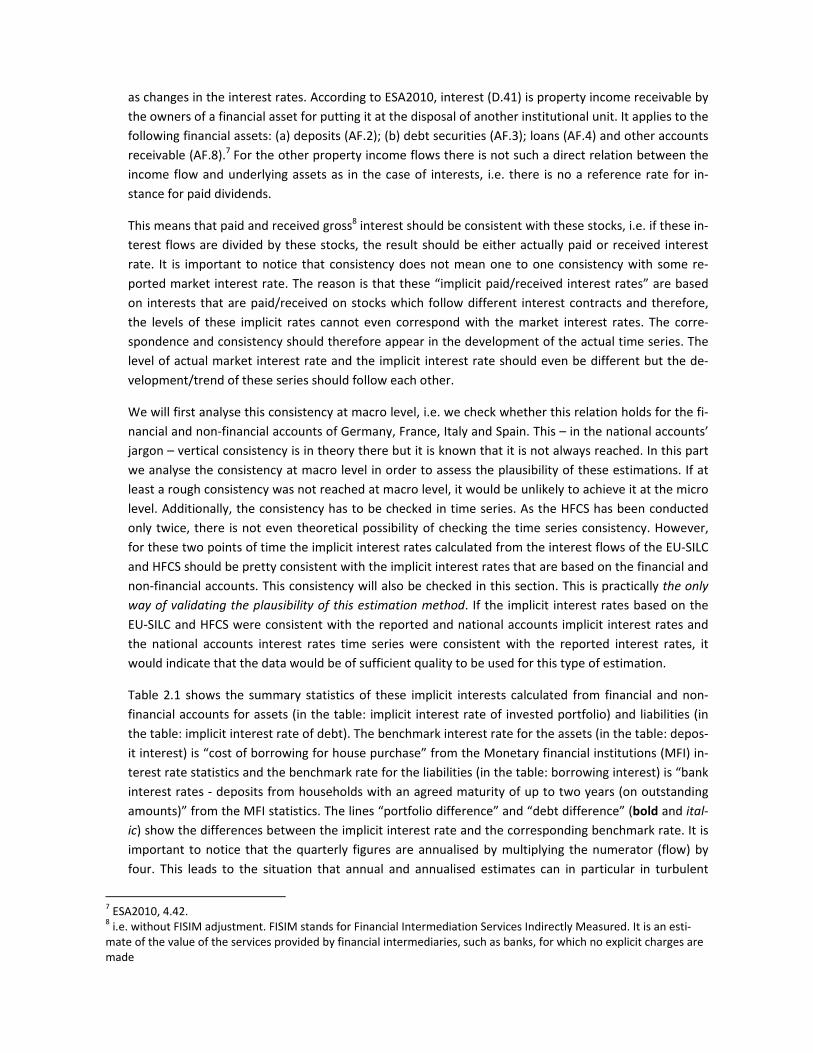
This means that paid and received gross8 interest should be consistent with these stocks, i.e. if these in‐

terest flows are divided by these stocks, the result should be either actually paid or received interest

rate. It is important to notice that consistency does not mean one to one consistency with some re‐

ported market interest rate. The reason is that these “implicit paid/received interest rates” are based

on interests that are paid/received on stocks which follow different interest contracts and therefore,

the levels of these implicit rates cannot even correspond with the market interest rates. The corre‐

spondence and consistency should therefore appear in the development of the actual time series. The

level of actual market interest rate and the implicit interest rate should even be different but the de‐

velopment/trend of these series should follow each other.

We will first analyse this consistency at macro level, i.e. we check whether this relation holds for the fi‐

nancial and non‐financial accounts of Germany, France, Italy and Spain. This – in the national accounts’

jargon – vertical consistency is in theory there but it is known that it is not always reached. In this part

we analyse the consistency at macro level in order to assess the plausibility of these estimations. If at

least a rough consistency was not reached at macro level, it would be unlikely to achieve it at the micro

level. Additionally, the consistency has to be checked in time series. As the HFCS has been conducted

only twice, there is not even theoretical possibility of checking the time series consistency. However,

for these two points of time the implicit interest rates calculated from the interest flows of the EU‐SILC

and HFCS should be pretty consistent with the implicit interest rates that are based on the financial and

non‐financial accounts. This consistency will also be checked in this section. This is practically the only

way of validating the plausibility of this estimation method. If the implicit interest rates based on the

EU‐SILC and HFCS were consistent with the reported and national accounts implicit interest rates and

the national accounts interest rates time series were consistent with the reported interest rates, it

would indicate that the data would be of sufficient quality to be used for this type of estimation.

Table 2.1 shows the summary statistics of these implicit interests calculated from financial and non‐

financial accounts for assets (in the table: implicit interest rate of invested portfolio) and liabilities (in

the table: implicit interest rate of debt). The benchmark interest rate for the assets (in the table: depos‐

it interest) is “cost of borrowing for house purchase” from the Monetary financial institutions (MFI) in‐

terest rate statistics and the benchmark rate for the liabilities (in the table: borrowing interest) is “bank

interest rates ‐ deposits from households with an agreed maturity of up to two years (on outstanding

amounts)” from the MFI statistics. The lines “portfolio difference” and “debt difference” (bold and ital‐

ic) show the differences between the implicit interest rate and the corresponding benchmark rate. It is

important to notice that the quarterly figures are annualised by multiplying the numerator (flow) by

four. This leads to the situation that annual and annualised estimates can in particular in turbulent

7 ESA2010, 4.42. 8 i.e. without FISIM adjustment. FISIM stands for Financial Intermediation Services Indirectly Measured. It is an esti‐mate of the value of the services provided by financial intermediaries, such as banks, for which no explicit charges are made

times differ from the annual figures. The analysis is done for time series from 2008q1 to 2017q4. This

time spam covers the both survey years as well as these data are most likely based on actual compila‐

tion methods rather than back data estimations.

Summary statistics show the minimum, the first quartile, the median (second quartile), the third quar‐

tile, and the maximum. From the analysis point of view, it is essential to focus on the portfolio and debt

differences. As mentioned earlier, there can and also should be differences vis‐à‐vis to the market in‐

terest rates but it is essential that differences are pretty constant. If the all these statistical indicators

are constant or roughly similar, it indicates that in the whole time series the differences are stable.

However, it is possible that there are for instance large differences in the last observations or alterna‐

tively, some individual outliers. From that point of view, it is not so worrying if the minimum and/or

maximum values are differing somewhat more as long as the first quartile, median and third quartile

values are roughly similar.

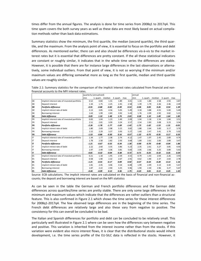
Table 2.1: Summary statistics for the comparison of the implicit interest rates calculated from financial and non‐financial accounts to the MFI interest rates.

Source: ECB calculations. The implicit interest rates are calculated on the basis of financial and non‐financial ac‐counts; the deposit and borrowing interest are based on the MFI statistics

As can be seen in the table the German and French portfolio differences and the German debt differences across quartiles/time series are pretty stable. There are only some large differences in the minimum and maximum values which indicate that the differences are rather outliers than a structural feature. This is also confirmed in Figure 2.1 which shows the time series for these interest differences for 2008q1‐2017q4. The few observed large differences are in the beginning of the time series. The French debt differences are relatively large and also these vary from negative to positive. The consistency for this can overall be concluded to be bad.

The Italian and Spanish differences for portfolio and debt can be concluded to be relatively small. This particularly well illustrated in Figure 2.1 where can be seen how the differences vary between negative and positive. This variation is inherited from the interest income rather than from the stocks. If this variation were evident also micro interest flows, it is clear that the distributional stocks would inherit development, i.e. the time series profile of the EU‐SILC data is reflected in the stocks. However, it

quarterly (annualised) annual

min 1. quart. median 3. quart. max min 1. quart. median 3. quart. max

DE Implicit interest rate of invested portfolio 0.52 0.84 1.55 1.89 3.01 1.33 1.84 2.58 2.93 3.87

DE Deposit interest 1.34 1.75 2.25 2.45 2.58 1.39 1.79 2.26 2.46 2.49

DE Portfolio difference ‐0.91 ‐0.88 ‐0.83 ‐0.49 0.53 ‐0.06 0.05 0.26 0.54 1.39

DE implicit intrest rate of debt 3.13 3.85 4.56 5.05 5.49 3.18 3.88 4.55 5.00 5.49

DE Borrowing interest 1.63 1.99 2.83 3.92 5.43 1.76 2.09 2.92 3.82 5.21

DE Debt difference 0.05 1.10 1.48 1.74 2.03 0.28 1.10 1.49 1.64 1.85

FR Implicit interest rate of invested portfolio 0.83 1.04 1.23 1.49 2.09 1.04 1.18 1.54 1.84 3.51

FR Deposit interest 2.51 2.81 3.09 3.24 3.57 2.54 2.83 3.08 3.23 3.54

FR Portfolio difference ‐2.26 ‐1.78 ‐1.77 ‐1.69 ‐1.42 ‐1.73 ‐1.62 ‐1.53 ‐1.31 ‐0.01

FR implicit intrest rate of debt 1.80 2.69 2.98 3.15 3.82 1.88 2.64 3.00 3.17 3.70

FR Borrowing interest 1.52 2.29 3.37 3.93 5.27 1.60 2.47 3.41 3.79 5.02

FR Debt difference ‐1.53 ‐0.86 ‐0.30 0.16 0.57 ‐1.32 ‐0.75 ‐0.35 0.17 0.35

IT Implicit interest rate of invested portfolio 1.34 1.77 2.38 2.74 4.12 1.47 1.97 2.45 2.89 4.74

IT Deposit interest 1.78 2.58 2.82 2.93 3.68 1.89 2.61 2.83 2.89 3.47

IT Portfolio difference ‐1.21 ‐0.67 ‐0.55 ‐0.34 1.30 ‐0.90 ‐0.70 ‐0.40 ‐0.04 1.86

IT implicit intrest rate of debt 2.22 2.60 3.35 3.86 5.23 2.35 2.61 3.27 3.85 4.93

IT Borrowing interest 1.97 2.49 3.36 3.81 5.83 2.05 2.66 3.25 3.89 5.63

IT Debt difference ‐0.81 ‐0.32 ‐0.04 0.38 0.72 ‐0.71 ‐0.25 ‐0.10 0.35 0.59

ES Implicit interest rate of invested portfolio 0.21 1.18 1.95 2.59 3.55 0.79 1.43 2.04 2.26 3.93

ES Deposit interest 0.58 1.90 2.32 2.67 2.91 0.62 1.90 2.37 2.64 2.78

ES Portfolio difference ‐1.21 ‐0.55 ‐0.17 0.09 0.92 ‐0.57 ‐0.33 ‐0.28 ‐0.13 1.16

ES implicit intrest rate of debt 1.81 2.45 3.06 3.54 6.08 1.99 2.49 3.13 3.44 5.67

ES Borrowing interest 1.87 2.22 2.90 3.25 5.96 1.90 2.30 2.96 3.27 5.67

ES Debt difference ‐0.44 ‐0.09 0.12 0.36 1.75 ‐0.23 0.01 0.13 0.25 1.45

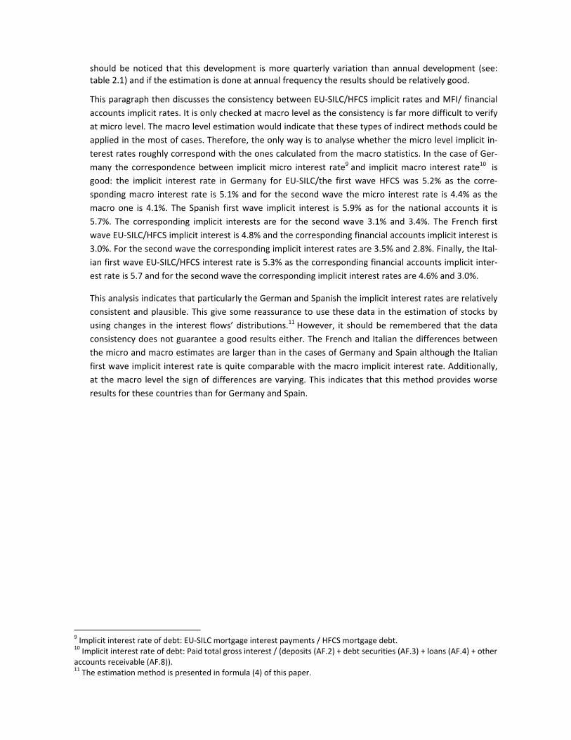
should be noticed that this development is more quarterly variation than annual development (see: table 2.1) and if the estimation is done at annual frequency the results should be relatively good.

This paragraph then discusses the consistency between EU‐SILC/HFCS implicit rates and MFI/ financial

accounts implicit rates. It is only checked at macro level as the consistency is far more difficult to verify

at micro level. The macro level estimation would indicate that these types of indirect methods could be

applied in the most of cases. Therefore, the only way is to analyse whether the micro level implicit in‐

terest rates roughly correspond with the ones calculated from the macro statistics. In the case of Ger‐

many the correspondence between implicit micro interest rate9 and implicit macro interest rate10 is

good: the implicit interest rate in Germany for EU‐SILC/the first wave HFCS was 5.2% as the corre‐

sponding macro interest rate is 5.1% and for the second wave the micro interest rate is 4.4% as the

macro one is 4.1%. The Spanish first wave implicit interest is 5.9% as for the national accounts it is

5.7%. The corresponding implicit interests are for the second wave 3.1% and 3.4%. The French first

wave EU‐SILC/HFCS implicit interest is 4.8% and the corresponding financial accounts implicit interest is

3.0%. For the second wave the corresponding implicit interest rates are 3.5% and 2.8%. Finally, the Ital‐

ian first wave EU‐SILC/HFCS interest rate is 5.3% as the corresponding financial accounts implicit inter‐

est rate is 5.7 and for the second wave the corresponding implicit interest rates are 4.6% and 3.0%.

This analysis indicates that particularly the German and Spanish the implicit interest rates are relatively

consistent and plausible. This give some reassurance to use these data in the estimation of stocks by

using changes in the interest flows’ distributions.11 However, it should be remembered that the data

consistency does not guarantee a good results either. The French and Italian the differences between

the micro and macro estimates are larger than in the cases of Germany and Spain although the Italian

first wave implicit interest rate is quite comparable with the macro implicit interest rate. Additionally,

at the macro level the sign of differences are varying. This indicates that this method provides worse

results for these countries than for Germany and Spain.

9 Implicit interest rate of debt: EU‐SILC mortgage interest payments / HFCS mortgage debt. 10 Implicit interest rate of debt: Paid total gross interest / (deposits (AF.2) + debt securities (AF.3) + loans (AF.4) + other accounts receivable (AF.8)). 11 The estimation method is presented in formula (4) of this paper.

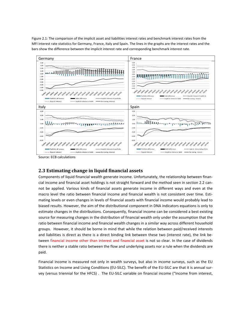
Figure 2.1: The comparison of the implicit asset and liabilities interest rates and benchmark interest rates from the

MFI interest rate statistics for Germany, France, Italy and Spain. The lines in the graphs are the interest rates and the

bars show the difference between the implicit interest rate and corresponding benchmark interest rate.

Germany France

Italy Spain

Source: ECB calculations

2.3EstimatingchangeinliquidfinancialassetsComponents of liquid financial wealth generate income. Unfortunately, the relationship between finan‐

cial income and financial asset holdings is not straight forward and the method seen in section 2.2 can‐

not be applied. Various kinds of financial assets generate income in different ways and even at the

macro level the ratio between financial income and financial wealth is not consistent over time. Esti‐

mating levels or even changes in levels of financial assets with financial income would probably lead to

biased results. However, the aim of the distributional component in DNA indicators equations is only to

estimate changes in the distributions. Consequently, financial income can be considered a best existing

source for measuring changes in the distribution of financial wealth only under the assumption that the

ratio between financial income and financial wealth changes in a similar way across different household

groups. However, it should be borne in mind that while the relation between paid/received interests

and liabilities is direct as there is a direct binding link between these two (interest rate), the link be‐

tween financial income other than interest and financial asset is not so clear. In the case of dividends

there is neither a stable ratio between the flow and underlying assets nor a rule when the dividends are

paid.

Financial income is measured not only in wealth surveys, but also in income surveys, such as the EU

Statistics on Income and Living Conditions (EU‐SILC). The benefit of the EU‐SILC are that it is annual sur‐

vey (versus triennial for the HFCS) . The EU‐SILC variable on financial income (“Income from interest,

dividends, and profit from capital investments in unincorporated business12”) is an aggregate of all in‐

come components of liquid financial wealth. This doesn’t allow a distinction between different ways

various wealth items generate income. Consequently, we need to assume that changes in this aggre‐

gate income variable reflect the distributional changes of wealth for each instrument individually. As re‐

ferred above, the fact that received interests and other financial income cannot be separated weakens

the assumption of this calculation.

Another limitation in survey data is that income from sight accounts is usually very limited at times of

low interest rates and may be significantly underreported. This assumption is supported by comparing

the shares of households receiving financial income to households owning various types of financial as‐

sets in the HFCS data. The former share is in all four countries lower than the share of households own‐

ing liquid financial assets (including sight accounts), but close to the share of households owning types

of liquid financial assets other than sight accounts.

Given this observation, we apply a model where the changes in the distribution of financial income (IS

in equation 4) are used to estimate changes in savings accounts, mutual funds, bonds and quoted

shares. For the estimation of the distribution of sight accounts, we use the last known distribution, ap‐

plying equation 213.

2.4EstimatingchangeinliabilitiesAs discussed in Chapter 2.2, interest payments on loans can be used to estimate the debt stock of the

household. For this analysis a distinction between mortgage and non‐mortgage debt would be useful

due to differences in interest rates levels between these types of debt. At the macro level, financial ac‐

counts do not allow such a distinction, but statistics on balance sheet items of monetary and financial

institutions (MFI BSI) enable a distinction between mortgages taken to purchase the household main

residence (HMR) and other loans. To maintain the levels of debt consistent with the levels of assets, we

take the value of total household debt from FA. In addition, we apply the portfolio structure of debt

from MFI BSI statistics to the FA data to enable a distinction between mortgages and non‐mortgage

loans in our analysis.

Information on interest payments on the mortgage taken to purchase the HMR is collected in EU‐SILC

and can be used as a proxy for HMR mortgages. As indicated earlier, the relationship between interest

payments on mortgages and the stock of mortgages is pretty stable at the macro level, and survey in‐

formation on this relationship is consistent with the macro data. On the other hand, no feasible proxy

can be found for non‐mortgage loans. Since HMR mortgages account for 2/3 of households’ liabilities in

the euro area, we can expect to improve the estimation significantly by estimating the changes in the

distribution of this component only. We apply the changes in interest payments on mortgage from EU‐

SILC (IS in equation 4) to estimate the change in the distribution of HMR mortgage debt by household

groups. For other loans, we apply the past distribution, i.e. equation 2.

12 Survey definition: “Interest (not included in the profit/loss of an unincorporated enterprise), dividends, profits from

capital investment in an unincorporated business refer to the amount of interest from assets such as bank accounts, certificates of deposit, bonds, etc., dividends and profits from capital investment in an unincorporated business, in which the person does not work, received during the income reference period (less expenses incurred).”(European Commission 2017) 13 Sight accounts could also be estimated reflecting changes in net income, but this approach did not improve the es‐timations.

3. EstimationatthemicrolevelMicrosimulation constitutes another option: this technique consists of simulating the effect of recent

macroeconomic changes on households at the micro level, in order to draw conclusions that apply to

higher levels of aggregation. In this section, we replicate the model implemented by Ampudia et al.

(2014) which has the advantage of being rather simple and transparent. The model is composed of a

mechanical extension of assets, income and debt, as well as a modelling part accounting for changes in

unemployment. This model will simulate both the changes in the value of assets and debt, as well

changes in the composition of income quintiles. As a second step, we estimate the changes in the port‐

folio structure not captured in the first step.14

We will consider the variable of interest: debt‐to‐liquid financial wealth (DTLFW) –ratio by income quin‐

tile, as well as its components, as defined in the previous Chapter.

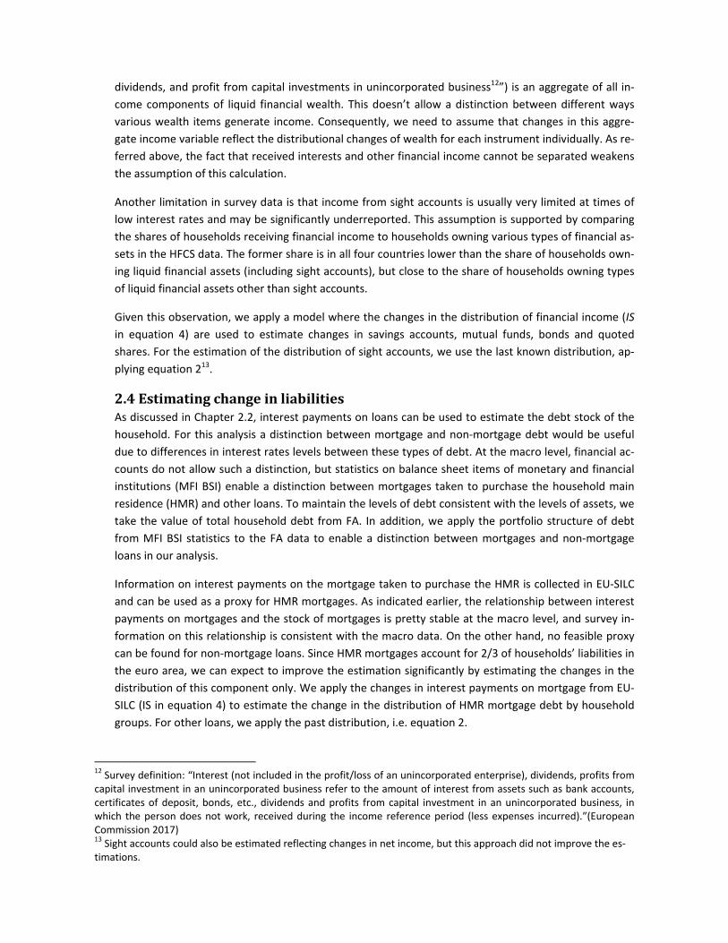
3.1UpdatingHFCSusingaggregatedataFirst, we mechanically update one by one the various assets, income components and rate of debt ser‐

vices with their country level aggregate, as described in table 3.1. In particular, house price indexes are

used to update real estate value; for the other asset types, indexes of quoted and unquoted stocks and

bonds are used. For the liabilities, we assume that debt is constant in real terms.

For debt services, we proceed as follows. No adjustment was made for fixed interest rate loan con‐

tracts; for adjustable‐rate mortgages, a complete pass‐through is assumed of the change in the interest

rate to the individual loan rate.

Table 3.1: Aggregate series used to extrapolate the balance sheet

14 See also:: Michelangeli and Pietrunti 2014. O’Donoghue and Loughrey 2014.

HFCS variable Aggregate Series Used to Extrapolate

Value of household’s main residence House price index

Value of other real estate property House price index

Value of household’s vehicles HICP

Valuables HICP

Value of self‐employment businesses Unquoted shares and other equity1

Deposits Deposits

Mutual funds Stock price index

Bonds Zero‐coupon‐bond price index

Value of non‐self‐employment private business Unquoted shares and other equity 1

Shares, publicly traded Stock price index

Managed accounts HICP

Money owed to households HICP

Other assets HICP

Voluntary pension/whole life insurance Insurance technical reserves

Employee income Wages per employee

Self‐employment income Gross operating surplus and mixed income2

Rental income from real estate property Gross operating surplus and mixed income2

Income from financial investments Interests

Income from pensions HICP

Regular social transfers (except pensions) HICP

Income from private transfers Miscellaneous current transfers2

Other income HICP

Total liabilities HICP

Payments for mortgages4 House purchase interest rate

Payments for non‐collaterised debt4 Consumption interest rate

1 Stock price index used for Germany

2 HICP used for countries with missing values

4 The increase in interest payments is calculated for the outstanding amounts of debt using formula (1).

Real assets

Financial Assets

Income

Debt and Financial Pressure

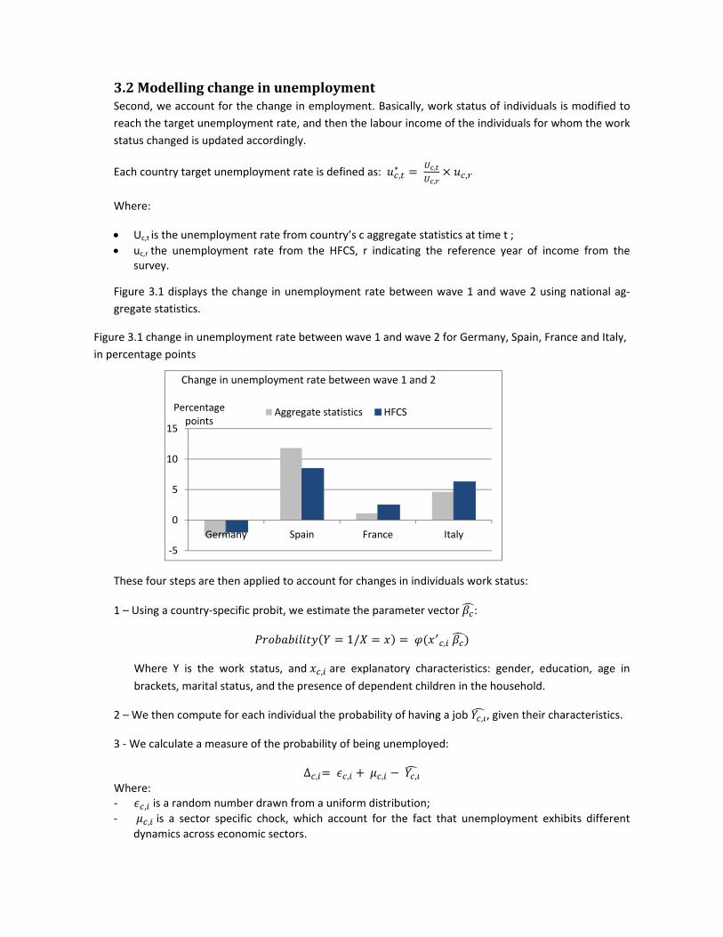
3.2ModellingchangeinunemploymentSecond, we account for the change in employment. Basically, work status of individuals is modified to

reach the target unemployment rate, and then the labour income of the individuals for whom the work

status changed is updated accordingly.

Each country target unemployment rate is defined as: ,∗ ,

,,

Where:

Uc,t is the unemployment rate from country’s c aggregate statistics at time t ;

uc,r the unemployment rate from the HFCS, r indicating the reference year of income from the survey.

Figure 3.1 displays the change in unemployment rate between wave 1 and wave 2 using national ag‐

gregate statistics.

Figure 3.1 change in unemployment rate between wave 1 and wave 2 for Germany, Spain, France and Italy,

in percentage points

These four steps are then applied to account for changes in individuals work status:

1 – Using a country‐specific probit, we estimate the parameter vector :

1/ ,

Where Y is the work status, and , are explanatory characteristics: gender, education, age in

brackets, marital status, and the presence of dependent children in the household.

2 – We then compute for each individual the probability of having a job , , given their characteristics.

3 ‐ We calculate a measure of the probability of being unemployed:

∆ , , , ,

Where: ‐ , is a random number drawn from a uniform distribution;

‐ , is a sector specific chock, which account for the fact that unemployment exhibits different

dynamics across economic sectors.

‐5

0

5

10

15

Germany Spain France Italy

Percentage points

Change in unemployment rate between wave 1 and 2

Aggregate statistics HFCS

4 – We use ∆ , to construct a ranking of the marginal probability of becoming unemployed. Using this

ranking, we determine the marginal employees losing their job/finding a job, so that the increase in the

simulated sample employment matches the change in the unemployment target.

Finally, for the individual for whom the work status changed, we update their income accordingly. For

the newly employed worker, we replace their current unemployment benefits with the predicted la‐

bour income15.When people become unemployed; we replace their current income with unemploy‐

ment benefits, using long‐term net replacement rates16.

3.3ModellingchangesintheportfolioThe model above estimates changes in assets and liabilities by applying macro level external infor‐

mation at the household level. While this is a feasible approach to estimate changes in the value of the

existing portfolios, it fails to capture any portfolio changes that probably occur particularly when

households experience income shocks.

As a follow‐up model, the simulated levels of financial assets are adjusted for changes in income be‐

tween the first wave (observed) and the second wave (simulated). This is done for both positive and

negative income shocks. First, we assume that household who experience a decrease in income com‐

pensate for this loss by selling liquid financial assets. The importance of the compensation is set as a

random percentage between 0 and 100% of the decrease in income, and does not take into account

the household saving rates17. Second, we assume that households who experience an increase in in‐

come will use part of this income (as above, a random percentage of the income increase) either to

purchase liquid financial assets or to pay off debt. The allocation between buying assets and paying off

debt is determined by the ratio between income and total debt. In both cases the increase/decrease in

LFW and debt is estimated at the instrument level, assuming an unchanged portfolio structure of LFW

and debt.

After the simulation has been conducted at the micro level, the distribution of LFW and debt is calcu‐

lated from the simulated data. This distribution is applied at the instrument level to the macro totals,

i.e. multiplying the macro aggregate with the wealth/debt share of each income quintile for each

wealth and debt component. The principle is shown in equation 3.

Combining the two models, one should be able to estimate the distributional changes caused by

changes in the value of assets, changes in the composition of income quintiles and changes in the port‐

folios of households’ financial wealth and debt caused by income shocks. However, the model does not

consider purchases and sales of real assets and consequently new or completely paid off mortgages.

15 The labour income is estimated using a two‐step Heckman selection model. The regressors are gender, education (dummies for having completed high school and having completed college) and age in brackets. 16 The net replacement rates vary along three dimensions: income, marital status, and presence of dependent chil‐dren. 17 The use of random compensation percentages is applied for simplicity. Households with medium or high saving rates may adjust consumption and/or saving instead. In the future the model could be developed to take into account household‐specific characteristics to determine the share of income loss compensated by selling financial wealth, by using e.g. regression models.

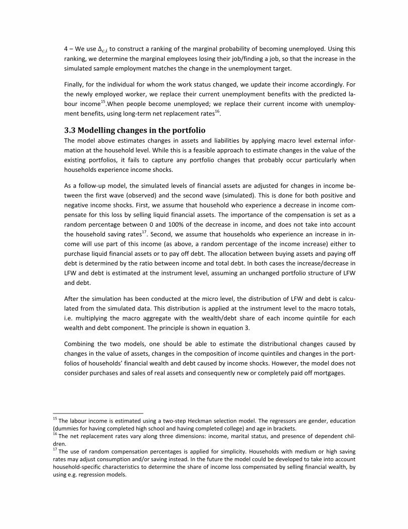
4. TheresultsTables 4.1 to 4.4 compare the results of the estimations for liquid financial wealth. The first column

shows the DNA indicator on per capita liquid financial wealth using the observed distributions from the

HFCS first wave18. Other columns indicate the changes in per capita LFW compared to HFCS wave 1, in

real terms. The second column uses the observed distributions from the HFCS second wave. This is the

‘true’ value used to assess the correctness of the estimations.

The third column (‘fixed distribution’) shows results from the macro estimation, applying wave 1 distri‐

butions at the instrument level to the financial accounts data of the wave 2 reference period. The

fourth column (‘estimated distribution’) shows the results from the meso‐level estimation, as described

in Chapter 2.3 and the rightmost column (‘Microsimulation’) shows the results from the microsimula‐

tion, as described in Chapter 3.

In the German HFCS, a large increase in the LFW of the second income quintile was observed, while the

LFW of the middle income classes declined. This is most probably due to the change in the composition

of the quintiles, where a number of relatively wealthy households experienced a negative income

shock. As expected, this was not captured by the macro or meso‐models, but the microsimulation

model produced very coherent results for the second quintile. On the other hand, the microsimulation

model underestimated the increase in LFW of income wealthy households.

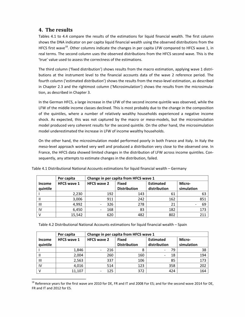
On the other hand, the microsimulation model performed poorly in both France and Italy. In Italy the

meso‐level approach worked very well and produced a distribution very close to the observed one. In

France, the HFCS data showed limited changes in the distribution of LFW across income quintiles. Con‐

sequently, any attempts to estimate changes in the distribution, failed.

Table 4.1 Distributional National Accounts estimations for liquid financial wealth – Germany

Income quintile

Per capita Change in per capita from HFCS wave 1

HFCS wave 1 HFCS wave 2 Fixed Distribution

Estimated distribution

Micro‐simulation

I 2,230 192 143 61 63

II 3,006 911 242 162 851

III 4,992 ‐ 326 278 21 ‐ 69

IV 6,450 ‐ 168 83 182 173

V 15,542 620 482 802 211

Table 4.2 Distributional National Accounts estimations for liquid financial wealth – Spain

Income quintile




Micro‐simulation

I 1,846 ‐ 216 8 ‐ 79 38

II 2,004 260 160 ‐ 18 194

III 2,563 337 106 85 173

IV 4,016 514 123 358 202

V 11,107 ‐ 125 372 424 164

18 Reference years for the first wave are 2010 for DE, FR and IT and 2008 For ES; and for the second wave 2014 for DE, FR and IT and 2012 for ES.

Table 4.3 Distributional National Accounts estimations for liquid financial wealth – France

Income quintile




Micro‐simulation

I 1,541 ‐ 67 51 206 816

II 2,292 ‐ 52 71 ‐ 170 519

III 3,182 67 102 ‐ 136 643

IV 4,886 427 151 ‐ 322 539

V 13,970 432 431 1,228 ‐ 1,712

Table 4.4 Distributional National Accounts estimations for liquid financial wealth – Italy

Income quintile




Micro‐simulation

I 1,753 ‐ 355 ‐ 31 ‐ 251 1,383

II 2,993 ‐ 71 ‐ 177 ‐ 29 267

III 4,930 ‐ 565 ‐ 347 ‐ 387 ‐ 189

IV 7,344 ‐ 424 ‐ 672 ‐ 632 ‐ 558

V 19,981 ‐ 1,378 ‐ 1,566 ‐ 1,494 ‐ 3,696

Tables 4.5 to 4.8 compare the results of the estimations for households’ liabilities, with similar contents

than in tables 4.1 to 4.4. In the case of liabilities, the performance of the estimation methods is rather

disappointing. The only exception is the meso‐level approach that produces a relatively close fit to the

observed distribution in Italy. Microsimulation does not produce accurate results in any country. In

Germany, where the developments of LFW in the low income groups were well estimated by microsim‐

ulation, the increase in liabilities in the second income quintile is not captured. In Italy, microsimulation

overestimates the debt levels of income poor households significantly.

Table 4.5 Distributional National Accounts estimations for liabilities – Germany

Income quintile




Micro‐simulation

I 676 ‐ 189 ‐ 43 25 ‐ 68

II 699 761 ‐ 37 ‐ 18 ‐ 15

III 2,908 ‐ 416 ‐ 97 ‐ 422 ‐ 14

IV 5,235 ‐ 191 ‐ 167 ‐ 124 ‐ 124

V 10,771 ‐ 658 ‐ 350 ‐ 153 ‐ 472

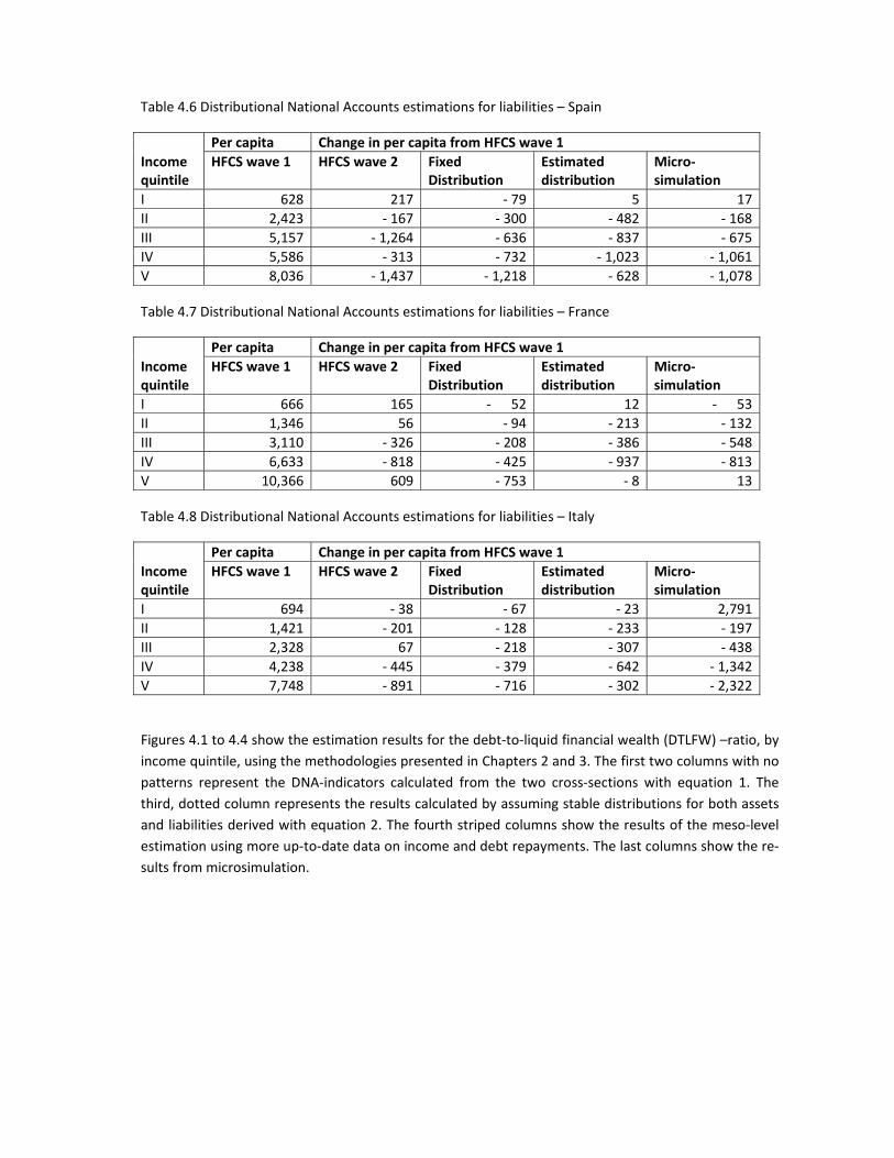
Table 4.6 Distributional National Accounts estimations for liabilities – Spain

Income quintile




Micro‐simulation

I 628 217 ‐ 79 5 17

II 2,423 ‐ 167 ‐ 300 ‐ 482 ‐ 168

III 5,157 ‐ 1,264 ‐ 636 ‐ 837 ‐ 675

IV 5,586 ‐ 313 ‐ 732 ‐ 1,023 ‐ 1,061

V 8,036 ‐ 1,437 ‐ 1,218 ‐ 628 ‐ 1,078

Table 4.7 Distributional National Accounts estimations for liabilities – France

Income quintile




Micro‐simulation

I 666 165 ‐ 52 12 ‐ 53

II 1,346 56 ‐ 94 ‐ 213 ‐ 132

III 3,110 ‐ 326 ‐ 208 ‐ 386 ‐ 548

IV 6,633 ‐ 818 ‐ 425 ‐ 937 ‐ 813

V 10,366 609 ‐ 753 ‐ 8 13

Table 4.8 Distributional National Accounts estimations for liabilities – Italy

Income quintile




Micro‐simulation

I 694 ‐ 38 ‐ 67 ‐ 23 2,791

II 1,421 ‐ 201 ‐ 128 ‐ 233 ‐ 197

III 2,328 67 ‐ 218 ‐ 307 ‐ 438

IV 4,238 ‐ 445 ‐ 379 ‐ 642 ‐ 1,342

V 7,748 ‐ 891 ‐ 716 ‐ 302 ‐ 2,322

Figures 4.1 to 4.4 show the estimation results for the debt‐to‐liquid financial wealth (DTLFW) –ratio, by

income quintile, using the methodologies presented in Chapters 2 and 3. The first two columns with no

patterns represent the DNA‐indicators calculated from the two cross‐sections with equation 1. The

third, dotted column represents the results calculated by assuming stable distributions for both assets

and liabilities derived with equation 2. The fourth striped columns show the results of the meso‐level

estimation using more up‐to‐date data on income and debt repayments. The last columns show the re‐

sults from microsimulation.

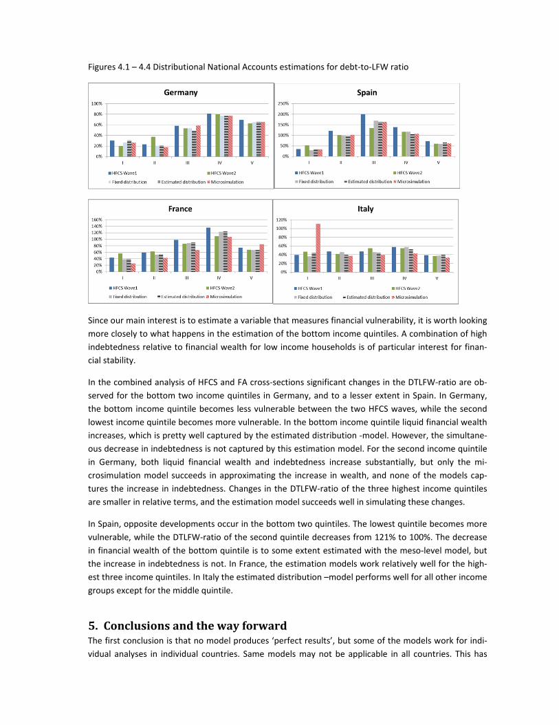
Figures 4.1 – 4.4 Distributional National Accounts estimations for debt‐to‐LFW ratio

Since our main interest is to estimate a variable that measures financial vulnerability, it is worth looking

more closely to what happens in the estimation of the bottom income quintiles. A combination of high

indebtedness relative to financial wealth for low income households is of particular interest for finan‐

cial stability.

In the combined analysis of HFCS and FA cross‐sections significant changes in the DTLFW‐ratio are ob‐

served for the bottom two income quintiles in Germany, and to a lesser extent in Spain. In Germany,

the bottom income quintile becomes less vulnerable between the two HFCS waves, while the second

lowest income quintile becomes more vulnerable. In the bottom income quintile liquid financial wealth

increases, which is pretty well captured by the estimated distribution ‐model. However, the simultane‐

ous decrease in indebtedness is not captured by this estimation model. For the second income quintile

in Germany, both liquid financial wealth and indebtedness increase substantially, but only the mi‐

crosimulation model succeeds in approximating the increase in wealth, and none of the models cap‐

tures the increase in indebtedness. Changes in the DTLFW‐ratio of the three highest income quintiles

are smaller in relative terms, and the estimation model succeeds well in simulating these changes.

In Spain, opposite developments occur in the bottom two quintiles. The lowest quintile becomes more

vulnerable, while the DTLFW‐ratio of the second quintile decreases from 121% to 100%. The decrease

in financial wealth of the bottom quintile is to some extent estimated with the meso‐level model, but

the increase in indebtedness is not. In France, the estimation models work relatively well for the high‐

est three income quintiles. In Italy the estimated distribution –model performs well for all other income

groups except for the middle quintile.

5. ConclusionsandthewayforwardThe first conclusion is that no model produces ‘perfect results’, but some of the models work for indi‐

vidual analyses in individual countries. Same models may not be applicable in all countries. This has

been the approach by the OECD EG‐DNA, where each country should select a suitable model to assess

distributional developments, based on data availability and applicability at the national level.

The meso‐level approach applying estimated distributions at a household group level uses a very broad

measure of financial income that is applied at the instrument level. Furthermore, the relationship be‐

tween financial income and financial wealth is not very stable at the macro level. In spite of these limi‐

tations, the meso‐level approach works well in Italy and relatively well in Spain for the estimation of the

change in the distribution of liquid financial wealth. In Italy, the portfolio share of bonds and mutual

funds in LFW is clearly higher than in the other three countries. One may assume that income generat‐

ed by these assets is better covered by households surveys (vis‐à‐vis deposits), and thus changes in the

distribution of financial income provide a feasible proxy for changes in financial wealth.

In Germany, microsimulation provides very promising results that capture an unusually high increase in

liquid financial wealth of the second income quintile. This proves that accounting for income mobility

can be important. It is worth noticing that the microsimulation model produces relatively limited in‐

come mobility for Germany, only 5% of households in the second simulated income quintile were in

higher income groups in the first wave. But nevertheless, the model was able to estimate satisfactorily

the impact of income mobility on LFW distribution. In Italy, microsimulation overestimates income mo‐

bility. For example, more than 35% of households are estimated to move from upper income quintiles

to the bottom quintile. This explains the vast overestimation of both wealth and liabilities in QI.

In spite of good macro level coherence between interest paid and liabilities, neither the meso‐level es‐

timation nor microsimulation produce results that are very reliable. The key to improving the estima‐

tion of the distribution of liabilities is to find methods that take into account the sale or purchase of real

assets. Portfolio changes related to financial assets are assumedly limited. Households are rarely able

to increase their savings by a large margin even in the medium term, neither are they usually forced to

sell large amounts of assets to compensate for a sudden income loss. For liabilities, the story is differ‐

ent. Because liabilities are frequently collateralised by real estate assets, a household may take signifi‐

cant amounts of debt from one day to another, if it purchases e.g. its main residence. Similarly, if a

household changes its tenure status from owner to renter for any reason, its debt stock decreases from

up to several hundred thousand euros to zero overnight.

References

Albacete, N. and P. Fessler (2010):” Stress testing Austrian households”, Financial Stability report 19, June,

European Central Bank.

Ampudia, M., A. Pavlickova, J. Slacalek and E. Vogel (2014): ”Household heterogeneity in the Euro Area

since the onset of the great recession”, ECB Working Paper Series No 1705.

Andreasch, M., P. Fessler and P. Lindner (2013): “Linking Microdata and Macrodata on Austrian Household

Financial Wealth Using HFCS and Financial Accounts Data”. Statistiken, Special Issue, pp. 14‐23, Oester‐

reichische Nationalbank.

Bankowska, K., J. Honkkila, S. Pérez‐Duarte and L. Reynaert Lefebvre (2017): "Household vulnerability in the

euro area," IFC Bulletins chapters, in: Bank for International Settlements (ed.), Data needs and Statistics

compilation for macroprudential analysis, volume 46 Bank for International Settlements.

Bettocchi, A., C. Moriconi, E. Giarda, F. Orsini, R. Romeo (2016): “Assessing and Predicting Financial Vulner‐

ability of Italian Households: A Micro‐Macro Approach”, Prometeia.

Dettling, L. J.; S. Devlin‐Foltz; J. Krimmel; S. Pack and J.P. Thompson (2015): “Comparing Micro and Macro

Sources for Household Accounts in the United States: Evidence from the Survey of Consumer Finances”,

FEDS Working Paper No. 2015‐086, http://dx.doi.org/10.17016/FEDS.2015.086

Durier, S.; L. Richet‐Mastain and M. Vanderschelden (2012): “Une décomposition du compte de patrimoine

des ménages de la comptabilité nationale per categories de ménages en 2003”, Direction des Statistiques

Démographiques et Sociales N° F1204.

European Commission (2017): Methodological Guidelines and Description of EU‐SILC Target Variables. Eu‐

rostat, Directorate F Social Statistics.

European System of Accounts 2010 (ESA2010), Publications Office of European Union, Luxembourg 2013.

Honkkila, J. and Kavonius, I. K. (2013): “Micro and Macro Analysis on Household Income, Wealth and Saving

in the Euro Area”, ECB Working Paper Series No 1619.

Household Finance and Consumption Network (HFCN 2016): The Household Finance and Consumption Sur‐

vey: methodological report of the second wave. ECB Statistics Paper No 17, December 2016.

IMF/FSB report to the G‐20 Finance Ministers and Central Bank Governors,

http://www.financialstabilityboard.org/publications/r_091107e.pdf

Kavonius, I. K. and J. Honkkila (2016): ”Deriving Household Indebtedness Indicators by Linking Micro and Mac‐ro Balance Sheet Data”, Statistical Journal of the IAOS (International Association for Official Statistics), Issue 2016/32, pp 693‐708, IOS Press.

Kavonius, I.K. and V.‐M. Törmälehto (2010): “Integrating Micro and Macro Accounts – The Linkages between Euro Area Household Wealth Survey and Aggregate Balance Sheets for Households”, the 31st General Confer‐ence of the International Association for Research in Income and Wealth (IARIW) in St. Gallen, Switzerland, August 2010.

Krimmel, J., K. B. Moore, J. Sabelhaus, and P. Smith (2013): “The Current State of U.S. Household balance sheets”, Federal Reserve of Bank of Saint Louis Review, 95(5), 337‐359.

Michelangeli, V. and M. Pietrunti (2014): ”A microsimulation model to evaluate Italian households’ financial vulnerability”, International Journal of microsimulation (2014) 7(3) 53‐79.

O’Donoghue, C., J. Loughrey (2014): ”Nowcasting in microsimulation models: a methodological survey”, Jour‐nal of Artificial Societies and Social Simulation 17 (4) 12.

Stiglitz, J.E.; A. Sen & J‐P Fitoussi (2009): “Report by the Commission on the Measurement of Economic Per‐

formance and Social Progress”, www.stiglitz‐sen‐fitoussi.fr.

Vienna Memorandum, European Statistical System Committee, 26‐27 September 2016,

http://ec.europa.eu/eurostat/documents/7330775/7339365/DGINS+Memorandum+2016/4ebdf162‐1b20‐

4d9e‐a8c7‐ae880eca9afd

Zwijnenburg, J., S. Bournot and F. Giovannelli (2017), "Expert Group on Disparities in a National Accounts

Framework: Results from the 2015 Exercise", OECD Statistics Working Papers, No. 2016/10, OECD Publish‐

ing, Paris, https://doi.org/10.1787/2daa921e‐en.

Linking Macro and Micro Household Balance Sheet Data time ...

Documents

Transcript of Linking Macro and Micro Household Balance Sheet Data time ...