Linear System Identification in a Nonlinear Setting -

Nonparametric analysis of the nonlinear distortions

and their impact on the best linear approximation

J. Schoukens, M. Vaes, and R. Pintelon. Vrije Universiteit Brussel, dept. ELEC, Pleinlaan 2, 1050 Brussel, Belgium

E-mail: Johan.Schoukens@vub.ac.be

This is a postprint copy of the following article under IEEE copyright: Linear System Identification in a Nonlinear Setting:

Nonparametric Analysis of the Nonlinear Distortions and Their Impact on the Best Linear Approximation. J.Schoukens, M. Vaes,

and R. Pintelon. IEEE Control Systems Magazine, Volume: 36, Issue: 3, June 2016, pp. 38 - 69. DOI: 10.1109/MCS.2016.2535918

Linear system identification [1]-[4] is a basic step in modern control design approaches. Starting from experimental data, a

linear dynamic time-invariant model is identified to describe the relationship between the reference signal and the output of

the system. At the same time, the power spectrum of the unmodeled disturbances is identified to generate uncertainty bounds

on the estimated model.

Linear system identification is also used in other disciplines, for example vibrational analysis of mechanical systems, where it

is called modal analysis [5], [6]. Because linear time-invariant models are a basic model structure, linear system identification is

frequently used in electrical [7]-[10], electronic, chemical [11], civil [12], and also in biomedical applications [13]. It provides

valuable information to the design engineers in all phases of the design process.

Starting from the late 1960s, system identification tools have been developed to obtain parametric models to describe the

dynamic behavior of systems. A formal framework is set up to study the theoretical properties of the system identification

algorithms [1]-[3]. The consistency (does the estimated model converge to the true system as the amount of data grows?) and

the efficiency (is the uncertainty of the estimated model as small as possible?) are analyzed in detail. Underlying all these

results are the assumptions that the system to be modeled is linear and time invariant.

It is clear that these assumptions are often (mostly?) not met in real-life applications. Most systems are only linear to a

first approximation. Depending on the excitation level, the output is disturbed by nonlinear distortions so that the linearity

assumption no longer holds. This immediately raises doubts about the validity of the results obtained and validated by the

linear system identification framework. The term nonlinear distortions indicates that nonlinear systems with a (dominant) linear

term are considered. The deviations from the linear behavior are called nonlinear distortions.

arX

iv:1

804.

0958

7v1

[cs

.SY

] 2

5 A

pr 2

018

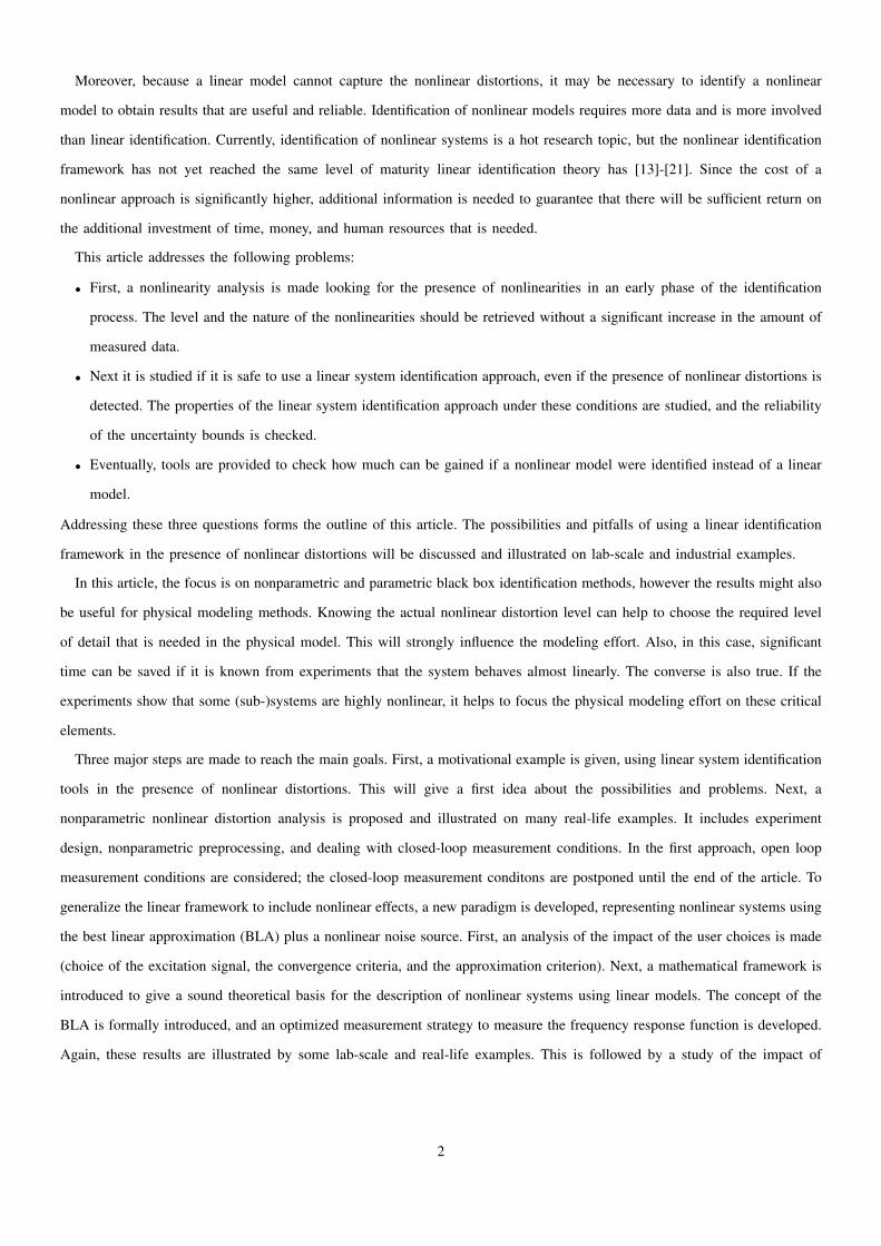
Moreover, because a linear model cannot capture the nonlinear distortions, it may be necessary to identify a nonlinear

model to obtain results that are useful and reliable. Identification of nonlinear models requires more data and is more involved

than linear identification. Currently, identification of nonlinear systems is a hot research topic, but the nonlinear identification

framework has not yet reached the same level of maturity linear identification theory has [13]-[21]. Since the cost of a

nonlinear approach is significantly higher, additional information is needed to guarantee that there will be sufficient return on

the additional investment of time, money, and human resources that is needed.

This article addresses the following problems:

• First, a nonlinearity analysis is made looking for the presence of nonlinearities in an early phase of the identification

process. The level and the nature of the nonlinearities should be retrieved without a significant increase in the amount of

measured data.

• Next it is studied if it is safe to use a linear system identification approach, even if the presence of nonlinear distortions is

detected. The properties of the linear system identification approach under these conditions are studied, and the reliability

of the uncertainty bounds is checked.

• Eventually, tools are provided to check how much can be gained if a nonlinear model were identified instead of a linear

model.

Addressing these three questions forms the outline of this article. The possibilities and pitfalls of using a linear identification

framework in the presence of nonlinear distortions will be discussed and illustrated on lab-scale and industrial examples.

In this article, the focus is on nonparametric and parametric black box identification methods, however the results might also

be useful for physical modeling methods. Knowing the actual nonlinear distortion level can help to choose the required level

of detail that is needed in the physical model. This will strongly influence the modeling effort. Also, in this case, significant

time can be saved if it is known from experiments that the system behaves almost linearly. The converse is also true. If the

experiments show that some (sub-)systems are highly nonlinear, it helps to focus the physical modeling effort on these critical

elements.

Three major steps are made to reach the main goals. First, a motivational example is given, using linear system identification

tools in the presence of nonlinear distortions. This will give a first idea about the possibilities and problems. Next, a

nonparametric nonlinear distortion analysis is proposed and illustrated on many real-life examples. It includes experiment

design, nonparametric preprocessing, and dealing with closed-loop measurement conditions. In the first approach, open loop

measurement conditions are considered; the closed-loop measurement conditons are postponed until the end of the article. To

generalize the linear framework to include nonlinear effects, a new paradigm is developed, representing nonlinear systems using

the best linear approximation (BLA) plus a nonlinear noise source. First, an analysis of the impact of the user choices is made

(choice of the excitation signal, the convergence criteria, and the approximation criterion). Next, a mathematical framework is

introduced to give a sound theoretical basis for the description of nonlinear systems using linear models. The concept of the

BLA is formally introduced, and an optimized measurement strategy to measure the frequency response function is developed.

Again, these results are illustrated by some lab-scale and real-life examples. This is followed by a study of the impact of

2

(a)1

ms2 ds k1s+ +-----------------------------------u y

k3y3

(b)

Figure 1. Forced Duffing oscillator (a): The electronic circuit mimics a nonlinear mechanical system with a hardening spring. Such a system is sometimescalled a forced Duffing oscillator. The system is excited with an input u(t) (the applied force to the mechanical system). The output of the system correspondsto the displacement y(t). The schematic representation of the system is given in (b) as a second-order system with a nonlinear feedback.

0 100 200

−0.2

0

0.2

Time (s)

Am

plitu

de (

V)

Figure 2. The system is excited with a low-pass signal, with a maximum excitation frequency of 200 Hz. The excitation signal consists of two parts. Thetail part consists of 10 sub-experiments. Each of these is a realization of a random signal, and will be used to estimate a linear model (Box-Jenkins structure)to model the data. The arrow-like part will be used to validate the estimated model. Observe that at the end of the arrow, the excitation level is larger thanthe tail amplitude. This gives the possibility to test the extrapolation capacity of the linear model.

nonlinear distortions on the parametric linear identification framework. At the end of the article, a short discussion about

publicly available software is given, followed by the conclusions.

This article is an extension of the keynote address that was given at The 13th International Workshop on Advanced Motion

Control AMC2014 [22].

A MOTIVATIONAL EXAMPLE

Consider the test setup in Figure 1. The electronic circuit mimics a nonlinear mechanical system with a hardening spring.

Such a system is sometimes called a forced Duffing oscillator [23], [24]. This class of nonlinear systems has a very rich

behavior, including regular and chaotic motions, and generation of subharmonics. The system is excited with an input u(t)

(the applied force to the mechanical system). The output of the system corresponds to the displacement y(t) .

This system can be schematically represented as a second-order system with a nonlinear feedback. It is excited with a

low-pass random excitation with a maximum excitation frequency of 200 Hz, as shown in Figures 2 and 3.

Modeling the nonlinear system using linear system identification tools

A linear approximating model will be estimated to describe the input-output relation of the system from the flat tail part.

3

0 100 200 300

−100

−50

0

Frequency (Hz)

Am

plitu

de (

dB)

(a)

0 100 200 300

−100

−50

0

Frequency (Hz)

Am

plitu

de (

dB)

(b)

Figure 3. The amplitude spectrum of the input (a) and output (b) signal. The spike at 250 Hz is a harmonic disturbance of the mains.

0 100 200 300−80

−60

−40

−20

0

20

Frequency (Hz)

Am

plitu

de (

dB)

Figure 4. The amplitude of the estimated transfer function model is shown (blue). Green line: the theoretic standard deviation of the estimated plant model,calculated from the estimated noise model. Red line: the actual observed standard deviation of the estimated plant model, estimated from the variations ofthe estimated plant model over the 10 subrecords. It can be seen that the actually observed standard deviation is underestimated with 4 dB by the theoreticalresults. This leads to too small error bounds.

The tail is split in 10 sub-records with a length of 8692 points, and each of these is used to identify a second-order discrete-

time plant model and a sixth-order noise model using the Box-Jenkins model structure of the prediction-error method [1], [2].

The estimated second-order plant transfer function, is shown in Figure 4.

Using this model, the output is ’simulated’. This is the identification term to indicate that the ouput is calculated from the

measured input. The simulation error, which is the difference between this simulated and measured output, is shown in Figure

5 (time domain) and Figure 6 (frequency domain) for the last subrecord. The latter shows also the 95% amplitude bound of

the simulation error that is calculated from the estimated sixth-order noise model. From these results it can be concluded that

a linear model gives still a reasonable approximation of the output of the nonlinear system. Moreover, the power spectrum of

the errors is well captured by the noise model, even if the dominating error is, in this case, the nonlinear distortions of the

system. That part of the nonlinear distortions that cannot be captured by the linear model is added to the noise disturbances

4

0 5 10

−0.2

0

0.2

Time (s)

Am

plitu

de (

V)

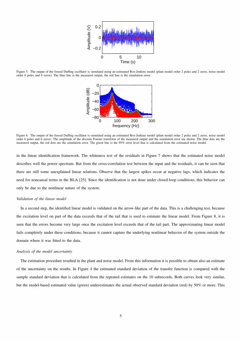
Figure 5. The output of the forced Duffing oscillator is simulated using an estimated Box-Jenkins model (plant model order 2 poles and 2 zeros, noise modelorder 6 poles and 6 zeros). The blue line is the measured output, the red line is the simulation error.

0 100 200 300−80

−60

−40

−20

0

frequency (Hz)

Am

plitu

de (

dB)

Figure 6. The output of the forced Duffing oscillator is simulated using an estimated Box-Jenkins model (plant model order 2 poles and 2 zeros, noise modelorder 6 poles and 6 zeros). The amplitude of the discrete Fourier transform of the measured output and the simulation error are shown. The blue dots are themeasured output, the red dots are the simulation error. The green line is the 95% error level that is calculated from the estimated noise model.

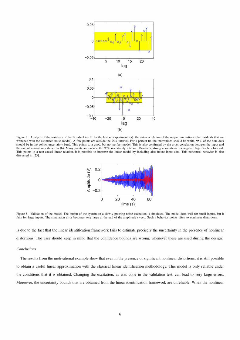
in the linear identification framework. The whiteness test of the residuals in Figure 7 shows that the estimated noise model

describes well the power spectrum. But from the cross-correlation test between the input and the residuals, it can be seen that

there are still some unexplained linear relations. Observe that the largest spikes occur at negative lags, which indicates the

need for noncausal terms in the BLA [25]. Since the identification is not done under closed-loop conditions, this behavior can

only be due to the nonlinear nature of the system.

Validation of the linear model

In a second step, the identified linear model is validated on the arrow-like part of the data. This is a challenging test, because

the excitation level on part of the data exceeds that of the tail that is used to estimate the linear model. From Figure 8, it is

seen that the errors become very large once the excitation level exceeds that of the tail part. The approximating linear model

fails completely under these conditions, because it cannot capture the underlying nonlinear behavior of the system outside the

domain where it was fitted to the data.

Analysis of the model uncertainty

The estimation procedure resulted in the plant and noise model. From this information it is possible to obtain also an estimate

of the uncertainty on the results. In Figure 4 the estimated standard deviation of the transfer function is compared with the

sample standard deviation that is calculated from the repeated estimates on the 10 subrecords. Both curves look very similar,

but the model-based estimated value (green) underestimates the actual observed standard deviation (red) by 50% or more. This

5

lag

(a)

lag(b)

Figure 7. Analysis of the residuals of the Box-Jenkins fit for the last subexperiment. (a): the auto-correlation of the output innovations (the residuals that arewhitened with the estimated noise model). A few points are outside the 95% interval. For a perfect fit, the innovations should be white, 95% of the blue dotsshould be in the yellow uncertainty band. This points to a good, but not perfect model. This is also confirmed by the cross-correlation between the input andthe output innovations shown in (b). Many points are outside the 95% uncertainty interval. Moreover, strong correlations for negative lags can be observed.This points to a non-causal linear relation, it is possible to improve the linear model by including also future input data. This noncausal behavior is alsodiscussed in [25].

0 20 40 60

−0.2

0

0.2

Time (s)

Am

plitu

de (

V)

Figure 8. Validation of the model. The output of the system on a slowly growing noise excitation is simulated. The model does well for small inputs, but itfails for large inputs. The simulation error becomes very large at the end of the amplitude sweep. Such a behavior points often to nonlinear distortions.

is due to the fact that the linear identification framework fails to estimate precisely the uncertainty in the presence of nonlinear

distortions. The user should keep in mind that the confidence bounds are wrong, whenever these are used during the design.

Conclusions

The results from the motivational example show that even in the presence of significant nonlinear distortions, it is still possible

to obtain a useful linear approximation with the classical linear identification methodology. This model is only reliable under

the conditions that it is obtained. Changing the excitation, as was done in the validation test, can lead to very large errors.

Moreover, the uncertainty bounds that are obtained from the linear identification framework are unreliable. When the nonlinear

6

distortions dominate the disturbing noise, significant underestimation of the variances appears. This problem will be analyzed

in more detail later in this article in the section on the parametric estimation of the BLA.

How to deal with nonlinear systems in system identification?

From these observations, the reader could decide that in the presence of nonlinear distortions it is better to build a complete

nonlinear model. But this choice is not without its own drawbacks. Nonlinear identification is more involved and often more

time consuming. This leads to more experiments and longer development times. Moreover, most engineers and designers are

often very familiar with linear design tools, but they are not trained in dealing with nonlinear systems. In many cases, imperfect

models with known error bounds are still very useful to make a design that meets the requested specifications. To follow this

strategy, tools are needed to detect in an early phase of the modeling process the presence of nonlinear distortions, and to

quantify their level. On the basis of this information, the design engineer can decide wether a cheaper linear identification

approach can be made, or if the more expensive nonlinear identification framework should be used. Using imperfect linear

models is not a problem as long as the user understands very well the validity of the linear models, and knows what will be

the impact of nonlinear distortions. The major goal of this article is to provide this background by discussing the three main

topics that were formulated at the end of the ’introduction section’: 1) Detection and characterization of nonlinear distortions;

2) Extending the linear framework to include the effect of nonlinear distortions; 3) Quantifying the potential gain by switching

from a linear to a nonlinear identification framework.

DETECTION, QUALIFICATION, AND QUANTIFICATION OF THE NONLINEAR DISTORTIONS

In this section tools will be presented that allow the user to detect and analyze the presence of nonlinear distortions during

the initial tests. Without needing more experiments, the frequency response function of the BLA, the power spectrum of the

disturbing noise, and the level of the nonlinear distortions will be obtained. All these results are obtained from a nonparametric

analysis, so that no user interaction is needed. At the basis of the proposed solution is the use of well-designed periodic

excitations. The restriction to periodic signals is the price to be paid to access all this information. The user can set the desired

frequency resolution and the desired power spectrum of the excitation signal. The phase will be chosen randomly on [0, 2π).

First, the response of a nonlinear system to a periodic excitation is studied, next it is explained how to design good periodic

excitation signals. Eventually, these signals will be used to make a nonparametric distortion and disturbing noise analysis.

The nonlinear distortion analysis is initially made under open-loop measurement conditions. The discussion of how to operate

under closed-loop conditions is postponed, because to do so the concept of ’BLA’, which will be introduced later in this article,

is needed

The response of a nonlinear system to a periodic excitation

A linear time-invariant system cannot transfer power from one frequency to another. In contrast, a nonlinear system can

transfer power from one frequency to another. Understanding this power transfer mechanism is an essential tool in the detection

and analysis of nonlinear distortions[26]. Consider a cosine signal passed through a cubic static nonlinear system y = u3

7

w1 2 301–2–

U w( )

(a)

1 1 1 31 1 -1 11 -1 1 11 -1 -1 -1

-1 1 1 1-1 1 -1 -1-1 -1 1 -1-1 -1 -1 -3

input outputfrequencyfrequency

(b)

w1 2 301–2–

Y w( )

3–

(c)

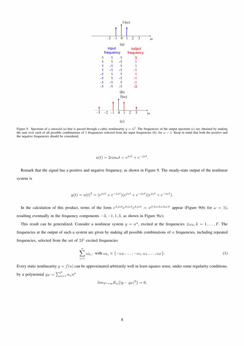
Figure 9. Spectrum of a sinosoid (a) that is passed through a cubic nonlinearity y = u3. The frequencies of the output spectrum (c) are obtained by makingthe sum over each of all possible combinations of 3 frequencies selected from the input frequencies (b), for ω = 1. Keep in mind that both the positive andthe negative frequencies should be considered.

u(t) = 2cosωt = ejωt + e−jωt.

Remark that the signal has a positive and negative frequency, as shown in Figure 9. The steady-state output of the nonlinear

system is

y(t) = u(t)3 = (ejωt + e−jωt)(ejωt + e−jωt)(ejωt + e−jωt).

In the calculation of this product, terms of the form e±jωte±jωte±jωt = ej(±ω±ω±ω)t appear (Figure 9(b) for ω = 1),

resulting eventually in the frequency components −3,−1, 1, 3, as shown in Figure 9(c).

This result can be generalized. Consider a nonlinear system y = uα, excited at the frequencies ±ωk, k = 1, . . . , F. The

frequencies at the output of such a system are given by making all possible combinations of α frequencies, including repeated

frequencies, selected from the set of 2F excited frequencies

α∑i=1

ωki , with ωki ∈ −ωF , . . . ,−ω1, ω1, . . . , ωF . (1)

Every static nonlinearity y = f(u) can be approximated arbitrarily well in least-squares sense, under some regularity conditions,

by a polynomial yP =∑Pα=1 aαu

α

limP→∞Eu|y − yP |2 = 0,

8

Gaussian noise periodic noise random multisine

time

frequency

(a) (b) (c)

(d) (e) (f)

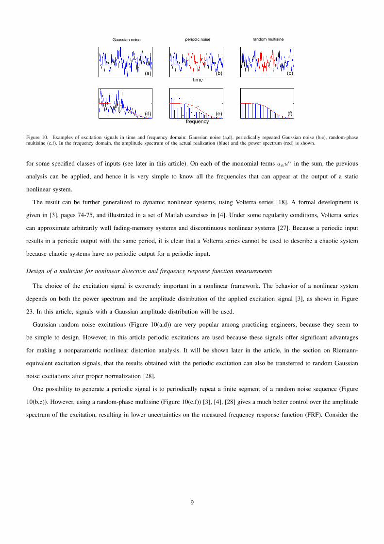
Figure 10. Examples of excitation signals in time and frequency domain: Gaussian noise (a,d), periodically repeated Gaussian noise (b,e), random-phasemultisine (c,f). In the frequency domain, the amplitude spectrum of the actual realization (blue) and the power spectrum (red) is shown.

for some specified classes of inputs (see later in this article). On each of the monomial terms aαuα in the sum, the previous

analysis can be applied, and hence it is very simple to know all the frequencies that can appear at the output of a static

nonlinear system.

The result can be further generalized to dynamic nonlinear systems, using Volterra series [18]. A formal development is

given in [3], pages 74-75, and illustrated in a set of Matlab exercises in [4]. Under some regularity conditions, Volterra series

can approximate arbitrarily well fading-memory systems and discontinuous nonlinear systems [27]. Because a periodic input

results in a periodic output with the same period, it is clear that a Volterra series cannot be used to describe a chaotic system

because chaotic systems have no periodic output for a periodic input.

Design of a multisine for nonlinear detection and frequency response function measurements

The choice of the excitation signal is extremely important in a nonlinear framework. The behavior of a nonlinear system

depends on both the power spectrum and the amplitude distribution of the applied excitation signal [3], as shown in Figure

23. In this article, signals with a Gaussian amplitude distribution will be used.

Gaussian random noise excitations (Figure 10(a,d)) are very popular among practicing engineers, because they seem to

be simple to design. However, in this article periodic excitations are used because these signals offer significant advantages

for making a nonparametric nonlinear distortion analysis. It will be shown later in the article, in the section on Riemann-

equivalent excitation signals, that the results obtained with the periodic excitation can also be transferred to random Gaussian

noise excitations after proper normalization [28].

One possibility to generate a periodic signal is to periodically repeat a finite segment of a random noise sequence (Figure

10(b,e)). However, using a random-phase multisine (Figure 10(c,f)) [3], [4], [28] gives a much better control over the amplitude

spectrum of the excitation, resulting in lower uncertainties on the measured frequency response function (FRF). Consider the

9

signal

u0 (t) =1√N

N/2−1∑k=−N/2+1

Ukej(2πkf0t+ϕk), (2)

=2√N

N/2−1∑k=−N/2+1

Ukcos (2πkf0t+ ϕk) , (3)

where ϕ−k = −ϕk and U−k = Uk, U0 = 0, and f0 = fs/N = 1/T . The sample frequency to generate the signal is fs, and T

is the period of the multisine. The phases ϕk will be selected independently such that Eejϕk = 0, for example by selecting

a uniform distribution on the interval [0, 2π). The amplitudes Uk are chosen to follow the desired amplitude spectrum (Figure

10(f)). See [28] for a detailed discussion about the user choices and the properties of these signals. The major advantage of the

random-phase multisine is that it still has (asymptotically for sufficiently large N ) all the nice properties of Gaussian noise,

while it also has the advantages of a deterministic signal: the amplitude spectrum does not show dips at the excited frequencies

(see Figure 10f)) as the two other signals do (see Figure 10(d) and (e)). At those dips, the measurements are very sensitive to

all nonlinear distortions and disturbing noise.

Remark

Initially, multisine excitations were introduced for the frequency response function (FRF) measurement of linear dynamic

systems [29]. To maximize the signal-to-noise ratio (SNR) of the measurements, an intensive search for compact signals

was made. For a given amplitude spectrum, the phases were chosen such that the peak value of the signal is minimized

[30]. Alternatively, well-designed binary signals could be used [31]. Although these compact signals are superior for linear

measurements, they are not so well suited to measure the FRF in the presence of nonlinear distortions. It will be explained in

this article (see Figure 23), that the linearized measurements depend strongly on the amplitude distribution of the excitation.

The specially designed multisines with a minimized peak factor have an amplitude distribution that is close to that of a sine

excitation (a high probability to be close to the extreme values, a low probability to be around zero, as shown in Figure

23). Random-phase multisines are asymptotically (with growing number of frequencies) Gaussian distributed, which is often

preferred in applications. Moreover, it will be possible to make explicit statements on the properties of the linear approximation

and the remaining errors for the latter case. For that reason, the focus will be from here on random-phase multisines and random

Gaussian excitations. More information on the impact of the amplitude distribution on the linear approximation can be found

in [32], [33].

User guidelines:

• Use random-phase multisine excitations.

• The spectral resolution f0 of the multisine should be chosen high enough so that no sharp resonances are missed [34].

Since f0 = 1/T , it sets immediately the period length T of the multisine. A high-frequency resolution requires a long

measurement time because at least one, and preferably a few, periods should be measured.

• The amplitude spectrum should be chosen such that the frequency band of interest is covered. The signal amplitude should

10

be scaled such that it also covers the input amplitude range of interest.

In the next section, it will be shown that nonlinear distortions can be easily detected by putting some amplitudes Uk in (2)

equal to zero for a well-selected set of frequencies.

A detailed step-by-step procedure of how to generate and process periodic excitations is given in Chapter 2 of [4].

Riemann-equivalent excitation signals

The goal is to characterize a nonlinear system for Gaussian excitation signals, using random-phase multisines. The design

of the amplitude spectrum of the multisine should be such that the equivalence between the random-phase multisine and the

Gaussian random noise with respect to the nonlinear behavior is guaranteed. To do so, the equivalence class ESU is defined

that collects all signals that are (asymptotically) Gaussian distributed, and have asymptotically, for N →∞, the same power

on each finite frequency interval. This is defined precisely in the next definition.

Definition 1. Riemann-equivalence class ESU of excitation signals. Consider a power spectrum SU (Ω) that is piecewise

continuous, with a finite number of discontinuities. A random signal belongs to the equivalence class if:

1) It is a Gaussian noise excitation with power spectrum SU (Ω),

2) It is a random multisine or random-phase multisine such that

1

N

kω2∑k=kω1

E(|U(k)|2) =1

2π

∫ ω2

ω1

SU (ν)dν +O(N−1) for all kωi ,

with

kωi = floor(ωi

2πfsN) and 0 < ω1, ω2 < πfs.

Using the Riemann equivalence, it is possible to use periodic random-phase multisines to characterize the properties of the

nonlinear system excited with filtered Gaussian noise. This will be explained in the next section.

Detection, separation, and characterization of the nonlinear distortions and the disturbing noise

This article presents only the basic principles of the nonlinear distortion analysis; see [3] for a more detailed discussion.

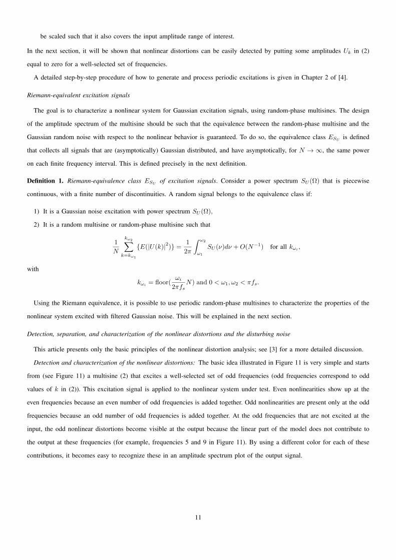
Detection and characterization of the nonlinear distortions: The basic idea illustrated in Figure 11 is very simple and starts

from (see Figure 11) a multisine (2) that excites a well-selected set of odd frequencies (odd frequencies correspond to odd

values of k in (2)). This excitation signal is applied to the nonlinear system under test. Even nonlinearities show up at the

even frequencies because an even number of odd frequencies is added together. Odd nonlinearities are present only at the odd

frequencies because an odd number of odd frequencies is added together. At the odd frequencies that are not excited at the

input, the odd nonlinear distortions become visible at the output because the linear part of the model does not contribute to

the output at these frequencies (for example, frequencies 5 and 9 in Figure 11). By using a different color for each of these

contributions, it becomes easy to recognize these in an amplitude spectrum plot of the output signal.

11

1 3 5 7 9 11

1 3 5 7 9 11 1 3 5 7 9 11

1 3 5 7 9 11

linear

even

odd

1 3 5 7 9 11

output

input

+

+

=

f f0¤ f f0¤

f f0¤

f f0¤

f f0¤

(a) (b)

(c)

(d)

(e)

Figure 11. Design of a multisine excitation for a nonlinear analysis. (a): Selection of the excited frequencies at the input (left side); At the output (rightside), from top to bottom: linear (b), even (c), odd (d) contributions, and total output (e).

Disturbing noise characterization: In the next step, the disturbing noise analysis is made. By analyzing the variations of the

periodic input and output signals over the measurements of the repeated periods, the sample mean and the sample (co-)variance

of the input and the output disturbing noise can be calculated, as a function of the frequency. Although the disturbing noise

varies from one period to the other, the nonlinear distortions do not, so they remain exactly the same. This results eventually

in the following simple procedure: consider the periodic signal u(t) in Figure 12. The periodic signal is measured over P

periods. For each subrecord, corresponding to a period, the discrete Fourier transform is calculated using the fast Fourier

transform (FFT) algorithm, resulting in the FFT spectra of each period U [l](k), Y [l](k), for l = 1, . . . , P . Because an integer

number of periods is measured, there will be no leakage in the results. The sample means U(k), Y (k) and noise (co)variances

σ2U (k), σ2

Y (k), σ2Y U (k) at frequency k are then given by

U(k) =1

P

P∑l=1

U [l](k) Y (k) =1

P

P∑l=1

Y [l](k),

and

σ2U (k) = 1

P−1∑Pl=1 |U [l](k)− U(k)|2,

σ2Y (k) = 1

P−1∑Pl=1 |Y [l](k)− Y (k)(k)|2,

σ2Y U (k) = 1

P−1∑Pl=1(Y (k)− Y (k))(U(k)− U(k))H .

(4)

In (4), (.)H denotes the complex conjugate. The variance of the estimated mean values U(k) and Y (k) is σ2U (k)/P and

σ2Y (k)/P, respectively. Adding together all this information in one figure results in a full nonparametric analysis of the system

with information about the system (the FRF), the even and odd nonlinear distortions, and the power spectrum of the disturbing

noise. Note that no interaction with the user is needed during the processing. This makes the method well suited to be

implemented in standard measurement procedures.

Combining multiple realizations of the random input: This measurement can be repeated over M realizations of the random-

phase multisine by generating each time a new multisine excitation with another random-phase realization. The results can

12

u t( )

u 1[ ] t( ) u 2[ ] t( ) u l[ ] t( )... ...t

Figure 12. Calculation of the sample mean and variance of a periodic signal.

then be averaged over these realizations to obtain more reliable estimates of the distortion and noise levels. At the same time,

the standard deviation of the FRF, due to the nonlinear distortions and the disturbing noise, will be reduced by√M .

In [35], [36], a detailed analysis is given of how these ideas can be generalized to deal with initial transient effects in SISO

and MIMO FRF measurements.

User guidelines

• Design a random multisine excitation following the guidelines specified earlier in this article.

• Excite the system with the multisine and measure P ≥ 2 periods of the steady-state response.

• Repeat this procedure for M successive realizations of the random-phase multisine.

• Choose P,M such that within the available measurement time the number of repetitions M is as large as possible. This

advice can be refined, depending on the prior knowledge of the user:

– No prior knowledge available: select P = 2, and M as large as possible.

– Maximize the nonlinear detection ability: M = 2, and P as large as possible.

– If it is known that the nonlinear distortions dominate: P = 1, and M as large as possible (the disturbing noise level

will not be estimated in this case).

CHARACTERIZING NONLINEAR DISTORTIONS: EXPERIMENTAL ILLUSTRATIONS

In this section, a series of experimental illustrations are presented. The first example is the forced Duffing oscillator that was

already used in the motivating example. The second and third examples are industrial applications (air path characterization

of a diesel engine, and a ground vibration test of an F-16 fighter).

Characterization of a forced Duffing oscillator: The nonlinear analysis method is experimentally illustrated on the electronic

circuit (see Figure 1, top) [3], [21], [37]. Although this is a nonlinear feedback system, it behaves as a fading-memory system

[27] for sufficiently small input amplitudes, and hence the proposed method can be applied.

The following settings were used to make the measurements: sample frequency is about 1220 Hz, the period length is 4096

samples, the frequency resolution is f0 ≈ 0.30 Hz, and the maximum excited frequency is 200 Hz. Only the odd frequencies

are excited, and in each block of 5 consecutive odd frequencies, the amplitude of one randomly selected frequency is put

to zero so that it can be used as a nonlinear detection line. All the excited frequencies have the same amplitude. For each

realization, 3 periods of the output were measured. The first period is dropped to avoid initial transient effects.

13

odd NL

even NL

noise

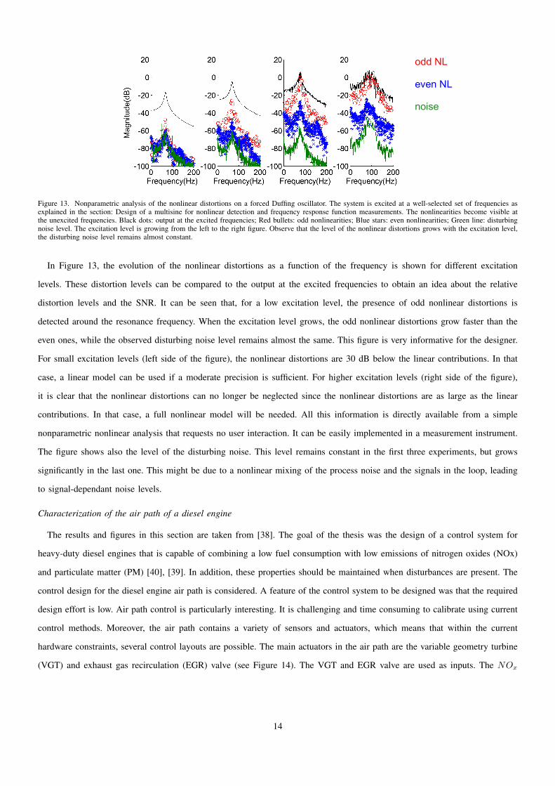
Figure 13. Nonparametric analysis of the nonlinear distortions on a forced Duffing oscillator. The system is excited at a well-selected set of frequencies asexplained in the section: Design of a multisine for nonlinear detection and frequency response function measurements. The nonlinearities become visible atthe unexcited frequencies. Black dots: output at the excited frequencies; Red bullets: odd nonlinearities; Blue stars: even nonlinearities; Green line: disturbingnoise level. The excitation level is growing from the left to the right figure. Observe that the level of the nonlinear distortions grows with the excitation level,the disturbing noise level remains almost constant.

In Figure 13, the evolution of the nonlinear distortions as a function of the frequency is shown for different excitation

levels. These distortion levels can be compared to the output at the excited frequencies to obtain an idea about the relative

distortion levels and the SNR. It can be seen that, for a low excitation level, the presence of odd nonlinear distortions is

detected around the resonance frequency. When the excitation level grows, the odd nonlinear distortions grow faster than the

even ones, while the observed disturbing noise level remains almost the same. This figure is very informative for the designer.

For small excitation levels (left side of the figure), the nonlinear distortions are 30 dB below the linear contributions. In that

case, a linear model can be used if a moderate precision is sufficient. For higher excitation levels (right side of the figure),

it is clear that the nonlinear distortions can no longer be neglected since the nonlinear distortions are as large as the linear

contributions. In that case, a full nonlinear model will be needed. All this information is directly available from a simple

nonparametric nonlinear analysis that requests no user interaction. It can be easily implemented in a measurement instrument.

The figure shows also the level of the disturbing noise. This level remains constant in the first three experiments, but grows

significantly in the last one. This might be due to a nonlinear mixing of the process noise and the signals in the loop, leading

to signal-dependant noise levels.

Characterization of the air path of a diesel engine

The results and figures in this section are taken from [38]. The goal of the thesis was the design of a control system for

heavy-duty diesel engines that is capable of combining a low fuel consumption with low emissions of nitrogen oxides (NOx)

and particulate matter (PM) [40], [39]. In addition, these properties should be maintained when disturbances are present. The

control design for the diesel engine air path is considered. A feature of the control system to be designed was that the required

design effort is low. Air path control is particularly interesting. It is challenging and time consuming to calibrate using current

control methods. Moreover, the air path contains a variety of sensors and actuators, which means that within the current

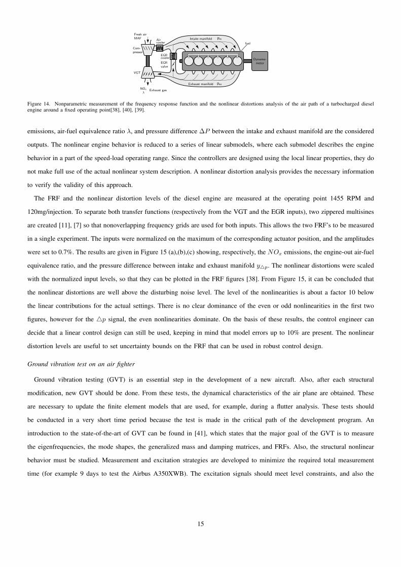
hardware constraints, several control layouts are possible. The main actuators in the air path are the variable geometry turbine

(VGT) and exhaust gas recirculation (EGR) valve (see Figure 14). The VGT and EGR valve are used as inputs. The NOx

14

EGRcooler

Aircooler

pin

pex

EGRvalve

VGT

NOx

λ

Com-pressor

Intake manifold

Exhaust manifold

Fresh airMAF

Dynamo-meter

fuel

Exhaust gas

Figure 14. Nonparametric measurement of the frequency response function and the nonlinear distortions analysis of the air path of a turbocharged dieselengine around a fixed operating point[38], [40], [39].

emissions, air-fuel equivalence ratio λ, and pressure difference ∆P between the intake and exhaust manifold are the considered

outputs. The nonlinear engine behavior is reduced to a series of linear submodels, where each submodel describes the engine

behavior in a part of the speed-load operating range. Since the controllers are designed using the local linear properties, they do

not make full use of the actual nonlinear system description. A nonlinear distortion analysis provides the necessary information

to verify the validity of this approach.

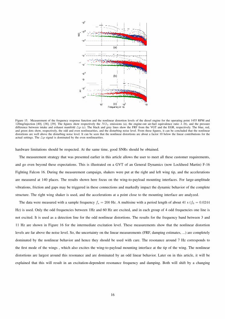
The FRF and the nonlinear distortion levels of the diesel engine are measured at the operating point 1455 RPM and

120mg/injection. To separate both transfer functions (respectively from the VGT and the EGR inputs), two zippered multisines

are created [11], [7] so that nonoverlapping frequency grids are used for both inputs. This allows the two FRF’s to be measured

in a single experiment. The inputs were normalized on the maximum of the corresponding actuator position, and the amplitudes

were set to 0.7%. The results are given in Figure 15 (a),(b),(c) showing, respectively, the NOx emissions, the engine-out air-fuel

equivalence ratio, and the pressure difference between intake and exhaust manifold y4p. The nonlinear distortions were scaled

with the normalized input levels, so that they can be plotted in the FRF figures [38]. From Figure 15, it can be concluded that

the nonlinear distortions are well above the disturbing noise level. The level of the nonlinearities is about a factor 10 below

the linear contributions for the actual settings. There is no clear dominance of the even or odd nonlinearities in the first two

figures, however for the 4p signal, the even nonlinearities dominate. On the basis of these results, the control engineer can

decide that a linear control design can still be used, keeping in mind that model errors up to 10% are present. The nonlinear

distortion levels are useful to set uncertainty bounds on the FRF that can be used in robust control design.

Ground vibration test on an air fighter

Ground vibration testing (GVT) is an essential step in the development of a new aircraft. Also, after each structural

modification, new GVT should be done. From these tests, the dynamical characteristics of the air plane are obtained. These

are necessary to update the finite element models that are used, for example, during a flutter analysis. These tests should

be conducted in a very short time period because the test is made in the critical path of the development program. An

introduction to the state-of-the-art of GVT can be found in [41], which states that the major goal of the GVT is to measure

the eigenfrequencies, the mode shapes, the generalized mass and damping matrices, and FRFs. Also, the structural nonlinear

behavior must be studied. Measurement and excitation strategies are developed to minimize the required total measurement

time (for example 9 days to test the Airbus A350XWB). The excitation signals should meet level constraints, and also the

15

(b)

(c)

(a)

Figure 15. Measurement of the frequency response function and the nonlinear distortion levels of the diesel engine for the operating point 1455 RPM and120mg/injection [40], [38], [39]. The figures show respectively the NOx emissions (a), the engine-out air-fuel equivalence ratio λ (b), and the pressuredifference between intake and exhaust manifold 4p (c). The black and grey lines show the FRF from the VGT and the EGR, respectively. The blue, red,and green dots show, respectively, the odd and even nonlinearities, and the disturbing noise level. From these figures, it can be concluded that the nonlineardistortions are well above the disturbing noise level. It can be seen that the nonlinear distortions are about a factor 10 below the linear contributions for theactual settings. The 4p signal is dominated by the even nonlinearities.

hardware limitations should be respected. At the same time, good SNRs should be obtained.

The measurement strategy that was presented earlier in this article allows the user to meet all these customer requirements,

and go even beyond these expectations. This is illustrated on a GVT of an General Dynamics (now Lockheed Martin) F-16

Fighting Falcon 16. During the measurement campaign, shakers were put at the right and left wing tip, and the accelerations

are measured at 140 places. The results shown here focus on the wing-to-payload mounting interfaces. For large-amplitude

vibrations, friction and gaps may be triggered in these connections and markedly impact the dynamic behavior of the complete

structure. The right wing shaker is used, and the accelerations at a point close to the mounting interface are analyzed.

The data were measured with a sample frequency fs = 200 Hz. A multisine with a period length of about 41 s (f0 = 0.0244

Hz) is used. Only the odd frequencies between 1Hz and 60 Hz are excited, and in each group of 4 odd frequencies one line is

not excited. It is used as a detection line for the odd nonlinear distortions. The results for the frequency band between 3 and

11 Hz are shown in Figure 16 for the intermediate excitation level. These measurements show that the nonlinear distortion

levels are far above the noise level. So, the uncertainty on the linear measurements (FRF, damping estimates, ...) are completely

dominated by the nonlinear behavior and hence they should be used with care. The resonance around 7 Hz corresponds to

the first mode of the wings , which also excites the wing-to-payload mounting interface at the tip of the wing. The nonlinear

distortions are largest around this resonance and are dominated by an odd linear behavior. Later on in this article, it will be

explained that this will result in an excitation-dependent resonance frequency and damping. Both will shift by a changing

16

(a)

5 10 15-80

-60

-40

-20

0

20

Frequency (Hz)

Am

plitu

de(d

B)

(b)

Figure 16. Ground vibration test on the General Dynamics F16 fighter jet (a). The right wing is excited with a shaker, and the accelerations are measured at140 places. In figure (b) the measured acceleration for a measurement point close to the right tip, near the missile connections, is shown. Black: output at theexcited frequencies, Red: odd nonlinear distortions, Blue: even nonlinear distortions, Green: disturbing noise level. These measurements show that the levelof the nonlinear distortions is well above the disturbing noise level.

excitation level.

Observe that the disturbing noise levels are at -40 to -60 dB which is very good for mechanical measurements. This illustrates

that the proposed measurement strategy meets all the formulated expectations for a good GVT. In a single experiment, it is

possible to measure the mode-shapes and the resonance frequencies, together with a full nonlinear signature of the nonlinear

behavior of the tested structure. The measured FRFs will be discussed later (see Figure 30).

NONLINEAR DISTORTIONS CHARACTERIZATION: ALTERNATIVE METHODS

In the first part of this article, a nonlinear distortion analysis method has been presented that strongly relies on the use

of random-phase multisines with a well-designed frequency grid. Alternative approaches to detect the presence of nonlinear

distortions are described in the survey article [51], and [52], with a focus on mechanical applications. Amongst others, the

following methods are discussed: superposition principle and homogeneity principle [53]; overlaid Bode plot and Nyquist plot

distortions [54]; coherence function measurements [42], [3]; bispectral analysis [55], [56]; Hilbert transform [57]; correlation

methods[58], [59].

This article discusses two alternative methods in more detail: the higher-order sinusoidal input describing functions (HOSIDFs),

and the swept sine test. There are three reasons for this choice: i) these methods can be considered as special cases of the

17

Figure 17. Experimental setup to analyze stick/sliding in a linear bearing with friction [62] .

previously presented framework in which the multisine signal is replaced by a single (swept) sine excitation; 2) The HOSIDFs

are an elegant and practical useful generalization of the concepts that are presented in this article; 3) The swept sine analysis

provides additional nonparametric information about the nonlinear distortion in mechanical vibrating systems.

Higher-order sinusoidal input describing functions

The HOSIDFs are a generalization of the sinusoidal input describing function [60], and describe the gain and phase relation

of a system between the input at the fundamental frequency f0 and the output at the harmonics kf0, using a sinusoidal input

signal [61]

Gk(f0, a) = Y (kf0)/Uks (f0),

where a indicates the amplitude of the excitation signal. The method can be used under feedback conditions [62]. The HOSIDFs

give a simple description of complex nonlinear behaviors of mechanical systems, for example, the transition from stick to sliding

in precision mechatronic systems [63].

An electromechanical shaker drives a sledge that is prone to dry friction mainly created by the dry friction finger, resulting

in a stick/slip behavior (see Figure 17) [63], [62], [61]. The driving current of the shaker is used as an input, and the measured

acceleration is the output of the system.

The amplitudes of the first- and third-order HOSIDFs are shown in Figure 18. As long as the system is in the stick phase,

it behaves as a linear system with a large stiffness. Once the sledge starts to move, nonlinear distortions become visible in

the measured acceleration, resulting in a large increase of the third-order HOSIDFs. This makes it possible to detect very

clearly the transition from stick to slip for varying excitation conditions (frequency and amplitude of the sine excitation).

These results show that the HOSIDFs are a versatile tool that provides intuitive insight in the behavior of a nonlinear system

that is directly accessible for the design engineer. It complements the multi-frequency tests that were explained before in the

section: Detection, separation, and characterization of the nonlinear distortions and the disturbing noise.

Swept sine test

The swept sine test works well for mechanical systems with isolated resonance modes, and the sensors positioned close

to the nonlinear component. The system is excited with a swept sine (this is a sine with constant amplitude, the frequency

18

(a)

(b)

Figure 18. Magnitude and phase of the first-order (a) and third-order (b) HOSIDFs for the system shown in the previous figure [62], [61], [63] .

varies linearly with time), and the presence of nonlinear distortions is looked for either by [64]: i) searching for anomalies in

the envelope of the response, ii) by plotting the acceleration against the relative displacement or relative velocity, or iii) by

making a time-frequency analysis using short-time Fourier transforms or a wavelet analysis. From these measurements, it is

also possible to make a first estimate of the function describing the local nonlinear component.

The sweep rate should be kept sufficiently low, such that the structure gets enough time to built up the full resonance

power when passing through a resonance. If only the acceleration signal is used in the analysis, sharp resonances might be

missed or strongly underestimated [66]. As a rule of thumb, the maximum sweep rate is proportional to ω23dB . This problem

disappears when the FRF is estimated from the input-output measurements [67], although even in this case the sweep rate

should remain low enough to have a good frequency resolution. As mentioned before, the frequency resolution is the inverse

of the measurement time. An increasing sweep rate decreases the measurement time required to cover a given frequency band,

and so the frequency resolution drops. In some standards, for example, the standard for space engineering testing [65], the

users are advised to use a logarithmic sweep rate between 2 or 4 octaves/min, independent of the structure. It is clear that

such a setting can become critical if the damping is too low.

These ideas are illustrated on the fighter measurements in Figure 19. A swept sine excitation, sweeping from 2 Hz to 15

Hz with a constant sweep rate of 0.05 Hz/s is applied to the wing. Figure 19(a) shows the measured acceleration of the wing

tip against the instantaneously swept sine frequency. The resonances that were already visible in Figure 16 and also in Figure

19

51015−5

0

5

Sweep frequency (Hz)

Acc

eler

atio

n (m

/s2 )

(a)

−4 −2 0 2 4

x 10−4

−5

0

5

Relative displacement (m)

− A

ccel

erat

ion

(m/s

2 )

(b)

Figure 19. Ground vibration test on the General Dynamics F16 fighter (see Figure 16) using a swept sine excitation. The accelerations on both sides ofthe bolted missile connection to the wing tip are measured. In (a), the measured acceleration is shown. In (b), the acceleration is plotted with respect to therelative displacement between the two sensors.

30 (which will be discussed later) show up also in Figure 16. In the plot the crossing of the instantaneous frequency through

the resonance at 7 Hz is highlighted in blue. Observe that this blue section is asymmetric, which is a strong indicator of the

presence of a nonlinear resonance. This part of the signal is further analyzed in Figure 16(b), plotting the measured acceleration

versus the relative displacement of two sensors put on the left and right side of the bolted connection. It is shown in [64] that

such a plot gives a good indication of the shape of the local stiffness. A detailed description and illustration on an aerospace

structure is given in [64]. The key idea is to discard all the inertia and force contributions that are not directly related to the

nonlinear component, as they are generally unknown or not measured. In Figure 19(b) a softening spring behavior is observed

(the acceleration is proportional to the force). This will be later confirmed by the FRF measurements shown in Figure 30.

In Figure 20, a time-frequency analysis is made of the acceleration signal and plotted as a function of the instantaneous

frequency (which replaces the time axis). The decreasing red line corresponds with the instantaneous swept sine frequency

applied to the fighter. Some harmonic frequencies are visible at the integer multiples of this frequency. Observe also that around

the resonance frequency, the intensity and the number of higher harmonics grows very fast. This points again to the presence

of a strong nonlinear behavior in the resonances.

This analysis complements well the multisine method that was explained before. It is applicable whenever local nonlinearities

are present, and it is possible to put sensors on both sides of the nonlinear structure.

20

Sweep frequency (Hz)

Inst

anta

neou

s fr

eq. (

Hz)

24681012140

20

40

60

80

100

Am

plitu

de (

dB)

−200

−180

−160

−140

−120

−100

−80

Figure 20. Time-frequency analysis of the measured acceleration signal at the tip of the wing [64].

SYSTEM IDENTIFICATION IN THE PRESENCE OF NONLINEAR DISTORTIONS: SELECTION OF A LINEAR OR NONLINEAR

MODELING APPROACH?

Using the nonparametric test procedure described in in the previous sections, the user gets a clear view on the presence and

the behavior of the nonlinear distortions. The procedure is formalized in a set of user guidelines:

• Design a random-phase multisine to detect the presence of nonlinear distortions following the guidelines of the multisine

design section. To do so, the even frequencies and a set of randomly selected odd frequencies should be put to zero.

The bandwidth, power spectrum, and peak amplitude should be similar to the signals that will be later on applied to the

model. See [28] for a detailed discussion.

• Make a series of (steady-state) measurements with varying amplitudes or offsets of the excitation signal that cover the

amplitude range of interest, and make the nonlinear analysis. More advanced signal processing methods can be used to

remove transient effects [68], [35], [36].

• If the nonlinear distortions are smaller than the specified level of accuracy of the model to be built, a linear design might

be sufficient. This will lead to the BLA of the nonlinear system. Otherwise, a more involved nonlinear model will be

needed. The BLA will be studied in detail later in this article.

• Be aware that the BLA varies in general as a function of the power spectrum and amplitude distribution of the excitation

signal. For that reason, the excitation signals during the experiments should match as well as possible the signals that

will be applied later on to the model as explained in the first bullet above.

• Detailed step-by-step instructions for a nonparametric nonlinear distortion analysis are given in Section 6.1 of [4], including

a set of routines to prepare the experiments and process the data.

APPROXIMATION OF NONLINEAR SYSTEMS: USER CHOICES

Once a nonparametric nonlinear distortion analysis is made, the user has to decide, on the basis of this information, if a

linear model will be sufficient to meet the modeling goals, or if it is instead necessary to use a nonlinear model. To make this

21

choice, it is important to understand the behavior of the linear modeling framework in the presence of nonlinear distortions.

Some of the theoretical properties that are obtained under the linear assumptions will no longer hold. The asymptotic properties

of the linear model that is estimated from a nonlinear system need to be verified, and the physical interpretation of the noise

model needs to be modified. For a formal mathematical framework, see "A mathematical framework for nonlinear systems".

Within this framework, it is possible to give a precise definition and interpretation of the BLA that will be identified under

these settings.

Describing a system with a model that is too simple results in model errors. These model errors depend upon some choices

that are implicitly or explicitly made by the user. To address these issues and to understand the results, it is necessary to line

up the user choices that are present in each identification strategy. It is dangerous if the user is not aware of these choices, or

if their impact is not well understood. The impact of the selected approximation criterion, related convergence criterion, and

the chosen excitation signal are discussed below.

Approximation methods

The quality of the fit of a model to a system, or to the data that describe this system, can be expressed by defining a

distance between the model and the data. This distance is called the approximation criterion or the cost function. The sum

of the absolute or the squared errors are two popular choices. A first possibility to find an ’optimal’ approximating model is

to minimize the selected cost function with respect to the model parameters for the given data set. If the model can exactly

describe a system, and the data are free of measurement error, the choice of the approximation criterion is not so critical as long

as it becomes zero with exact model parameters. The choice of the cost function that minimizes the impact of disturbing noise

(the combined effect of measurement noise and process noise), still assuming that the system is in the model set, is the topic of

system identification theory. This section is focussed on the alternative situation. It starts from exact data, but the model is too

simple to give an exact description of the system. This results in model errors, and the choice of the approximation criterion

will significantly impact on the behavior of the resulting model errors. The ideas are presented by analyzing a simple example.

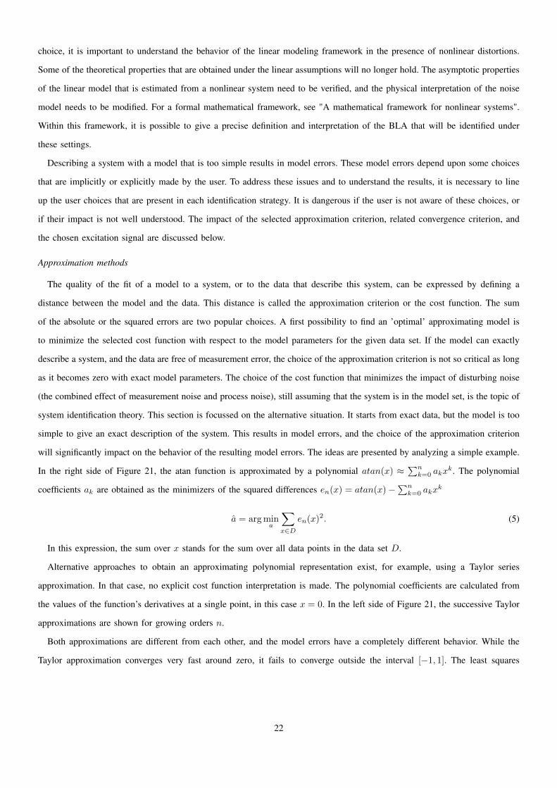
In the right side of Figure 21, the atan function is approximated by a polynomial atan(x) ≈∑nk=0 akx

k. The polynomial

coefficients ak are obtained as the minimizers of the squared differences en(x) = atan(x)−∑nk=0 akx

k

a = arg mina

∑x∈D

en(x)2. (5)

In this expression, the sum over x stands for the sum over all data points in the data set D.

Alternative approaches to obtain an approximating polynomial representation exist, for example, using a Taylor series

approximation. In that case, no explicit cost function interpretation is made. The polynomial coefficients are calculated from

the values of the function’s derivatives at a single point, in this case x = 0. In the left side of Figure 21, the successive Taylor

approximations are shown for growing orders n.

Both approximations are different from each other, and the model errors have a completely different behavior. While the

Taylor approximation converges very fast around zero, it fails to converge outside the interval [−1, 1]. The least squares

22

−2 0 2−2

0

2

u

atan

Tay

lor

−2 0 210

−20

100

1020

u

−2 0 2−2

0

2

u

atan

LS

−2 0 210

−20

100

1020

u

Figure 21. Illustration of the impact of the approximation criterion on the approximation errors. A static nonlinear system (blue line) is approximated using twodifferent approaches. That is, the comparison is between a Taylor series of order 1,3,5,7,9,11, and a polynomial model of order 1,3,5,7,9,11. The polynomialis fit using the least squares. The errors are shown in the bottom figures. Observe that the Taylor series approximation gives a much better fit around theorigin, but fails to converge for an input |u| > 1. The convergence of the least squares fit on the right side is much slower, but the approximation convergeseverywhere on the interval [-3,3].

approximation converges over the full interval [−3, 3] but at a slower rate. The width of the interval can be made arbitrarily

large.

In this article, the least squares model fitting approach is followed.

Convergence criteria

In the previous example, a polynomial approximation of the atan(x) function is made. Using the least-squares cost

function, the error can made arbitrarily small in a given interval by increasing the complexity of the model. In Figure 22,

a discontinuous function is approximated using polynomials of different degrees. Again, it can be seen that the error can be

made arbitrarily small for all inputs, except at the discontinuity at u = 0 where the error converges to half the discontinuity.

This prohibits uniform convergence that is characterized by a decrease of the maximum error in the interval. More formaly,

for all ε, there exists a value N such that supx∈D |en(x )| < ε for n > N.

To include also discontinuous functions in the framework, the convergence criterion should be weakened to point-wise

convergence, which can be obtained by using the convergence in the mean-square sense. Mean-square convergence requires

that

limn→∞

∑x∈D

en(x)2 = 0,

which guarantees that the approximation converges everywhere excepted for some isolated points where the function is

discontinuous. For continuous functions, uniform convergence is retrieved. It is clear that this concept matches very well

with the least-squares model-fitting approach.

In this article mean-square convergence will be used.

23

−2 0 2−2

0

2

u

Figure 22. Least-squares approximation of a discontinuous function with continuous basis functions.

Impact of the choice of the excitation signal

The actual fit of the model, in the absence of model errors and noise-free data, will not depend on the characteristics of the

excitation signal. This changes drastically when the model is not rich enough to capture the full system behavior. In that case,

errors will be present, and during the fit these will be pushed to those parts of the input domain that are not so well excited

because that reduces the cost in (5). This makes the results dependent on the choice of the excitation, which is illustrated in

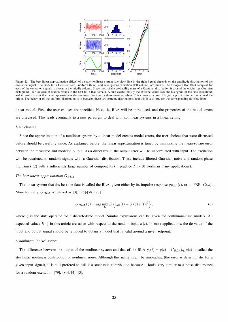
Figure 23 where atan(u) is linearly approximated using the model y = au. Figure 23 shows that the BLA depends on the

amplitude distribution of the excitation signal. The results for a Gaussian, uniform, and sine excitation (see left column) are

shown in the right figure. The histogram for each of the excitation signals is shown in the middle figures. Since most of the

probability mass of a Gaussian distribution is around the origin (see Gaussian histogram), the Gaussian excitation results in the

best fit in that sub-domain. A sine excites mostly the extreme values (see the histogram of the sine excitation), and it results

in a fit that better approximates the nonlinear function for these extreme values. This comes at a cost of larger approximation

errors around the origin. The behavior of the uniform distribution is in between these two extreme distributions, and this is

also true for the corresponding fit (blue line).

This example shows that the experiment design in the presence of model errors will be even more important than in classical

system identification where no model errors are considered. If the user is aware that model errors will be present, care should

be taken that at least a part of the experiment consists of signals that mimic very well the signals that will applied later on

to the model. The remaining part of the experiment can be used to obtain a sufficiently rich excitation so that the uncertainty

remains small enough. Such an approach is illustrated on the identification of an industrial clutch in [69]. To identify the

BLA for a nonlinear dynamic system, not only is the power spectrum of the excitation important (to cover the frequency band

of interest), also the amplitude distribution plays a crucial role (to excite those amplitude regions that will be used in later

applications). In [69], a mixture of random-phase multisines and impulsive excitations is used to cover the later use of the

model.

A NEW PARADIGM: REPLACING THE NONLINEAR SYSTEM BY A LINEAR SYSTEM PLUS A NOISE SOURCE

In the previous section, the impact of some user choices (approximation method, convergence criteria, excitation signal) on

the behavior of model errors is discussed. In this section, these results are used to approximate a nonlinear system with a

24

0 500 1000−5

0

5

Gau

ssia

n

0 500 1000−5

0

5

Uni

form

0 500 1000−5

0

5

Sin

e

time

−4 −2 0 2 40

200

400

−4 −2 0 2 40

200

400

−4 −2 0 2 40

200

400

amplitude−4 −2 0 2 4

−2

−1.5

−1

−0.5

0

0.5

1

1.5

2

input

Figure 23. The best linear approximation (BLA) of a static nonlinear system (the black line in the right figure) depends on the amplitude distribution of theexcitation signal. The BLA for a Gaussian (red), uniform (blue), and sine (green) excitation (left column) are shown. The histogram (for 1024 samples) foreach of the excitation signals is shown in the middle column. Since most of the probability mass of a Gaussian distribution is around the origin (see Gaussianhistogram), the Gaussian excitation results in the best fit in that domain. A sine excites mostly the extreme values (see the histogram of the sine excitation),and it results in a fit that better approximates the nonlinear function for these extreme values. This comes at a cost of larger approximation errors around theorigin. The behavior of the uniform distribution is in between these two extreme distributions, and this is also true for the corresponding fit (blue line).

linear model. First, the user choices are specified. Next, the BLA will be introduced, and the properties of the model errors

are discussed. This leads eventually to a new paradigm to deal with nonlinear systems in a linear setting.

User choices

Since the approximation of a nonlinear system by a linear model creates model errors, the user choices that were discussed

before should be carefully made. As explained before, the linear approximation is tuned by minimizing the mean-square error

between the measured and modeled output. As a direct result, the output error will be uncorrelated with input. The excitation

will be restricted to random signals with a Gaussian distribution. These include filtered Gaussian noise and random-phase

multisines (2) with a sufficiently large number of components (in practice F > 10 works in many applications).

The best linear approximation GBLA

The linear system that fits best the data is called the BLA, given either by its impulse response gBLA(t), or its FRF , G(ω).

More formally, GBLA is defined as [3], [75]-[78],[28]

GBLA (q) = arg minG

E|y0 (t)−G (q)u (t)|2

, (6)

where q is the shift operator for a discrete-time model. Similar expressions can be given for continuous-time models. All

expected values E in this article are taken with respect to the random input u (t). In most applications, the dc-value of the

input and output signal should be removed to obtain a model that is valid around a given setpoint.

A nonlinear ’noise’ source

The difference between the output of the nonlinear system and that of the BLA ys(t) = y(t)−GBLA(q)u(t) is called the

stochastic nonlinear contribution or nonlinear noise. Although this name might be misleading (the error is deterministic for a

given input signal), it is still prefered to call it a stochastic contribution because it looks very similar to a noise disturbance

for a random excitation [79], [80], [4], [3].

25

A new paradigm

By combining these results, the output of a nonlinear system that is driven by a random excitation (or a Riemann-equivalent

signal [28]) is split in two classes of contributions, being the coherent contributions YBLA and the noncoherent contributions

YS (see Figure 24). The linear part of the system contributes to the coherent output only, while the nonlinear distortions

contribute to both the coherent and noncoherent output.

• Coherent output: The relation between the input U0(k) and the coherent (non)linear contributions YBLA(k) is given by

YBLA(k) = GBLA(k)U(k) + T (k),

where T (k) models the transient effects and leakage errors [82], [3]. From now on it is assumed, without loss of generality,

that steady-state conditions apply, such that the transient terms can be neglected in what follows. The transfer function

GBLA(k) depends on the power spectrum of the Gaussian random excitation. Changing the Gaussian distribution to an

alternative such as a uniform distribution, can change the BLA. From a spectral point of view the phase of YBLA(k) is

equal to the phase of the input plus the phase of the transfer function GBLA(k). Since GBLA is an expected value over

the random input, its actual value will not depend upon the actual realization of the random input.

• Noncoherent output: The noncoherent output yS accounts for the difference between the output of the BLA and the

actual nonlinear output. For random excitations, it is very difficult for an untrained user to distinguish the nonlinear noise

yS (t) from the additive disturbing output noise v (t) (Figure 24). The nonlinear noise yS (t) is uncorrelated with u (t)

because they are the residuals of the solution of a least-squares problem. However, u (t) and yS (t) are mutually dependent

since there exists a nonlinear relation between both signals, namely

yS (t) = y0(t)−GBLA (q)u (t) .

Combining both results, the noise-free output y0 (t) can be written as the sum yBLA(t) + yS(t) (see Figure 24) [79], [80], [3]

y(t) = y0(t) + v(t),

y0 (t) = GBLA (q)u (t) + yS (t) . (7)

In the frequency domain the relation between the FFT spectra becomes

Y (k) =Y0 (k) + V (k)

=GBLA (k)U (k) + YS (k) + V (k) , (8)

disregarding again the transients T (k) representing the initial transients and leakage errors. The phase of YS(k) will depend

upon the phase of the input U(l), for some values l 6= k. This was not so for YBLA(k), whose phase depends only on the

input phase ∠U(k). Since the phases are stochastic variables, YS(k) will also be a stochastic value with respect to the random

26

Nonlinear Systemy0

yS

y0yBLAGBLA

u

u

Figure 24. A new paradigm: the nonlinear system (top figure) is replaced by the best linear approximation GBLA plus an error term yS(t) (bottom figure).

input.

The power spectra of YS and V can be measured using the nonparametric nonlinear detection methods that were explained

before. In [81] a rationale is given that shows that the level of the stochastic nonlinearities (noncoherent output) is also a good

indicator for the level of the nonlinear coherent output for the considered class of excitations (random-phase multisines and

Gaussian noise).

For the specified user choices (mean-square error, random Gaussian excitation), the asymptotic properties of GBLA and Ys

are well known, assuming that the number of frequencies N in the multisine (2) grows to infinity. A detailed discussion is

given in Section 3.4 of [3], here only a brief summary of the most important properties is given.

The BLA GBLA is shown to be smooth; it does not depend on N , and it is the same for all Riemann-equivalent excitations.

Only the odd nonlinearities contribute to GBLA.

The stochastic nonlinearities YS have a smooth power spectrum. They are zero-mean circular complex normally distributed,

and they have the same power spectrum for all Riemann-equivalent excitations. Both the even and the odd nonlinearities

contribute to YS .

A toy example

Consider a static nonlinear system

y =

n∑k=1

akuk.

For (filtered) Gaussian noise excitations, it is known from Bussgang’s theorem [78], that the BLA is also static yBLA = aBLAu.

The least-squares estimate is

aBLA =

∑y(t)u(t)∑u(t)2

,

which converges for large data sets to

aBLA =

n∑k=1

akµk+1/µ2,

with µα the moment of order α. This simple example shows that the BLA depends on the higher-order moments of the

excitation. Observe that this result depends only on the amplitude of the Gaussian noise (all higher-order moments of a zero-

mean Gaussian distribution are set by its variance), and not on its power spectrum. For zero-mean excitations, only the odd

degrees will contribute to the estimate.

27

0 0.2 0.4−6−4−2

024

f/fs

|GB

LA| (

dB)

uniform noise

0 0.2 0.4−20

0

20

f/fsar

g(G

BLA

) (o

)

0 0.2 0.4−6−4−2

024

f/fs

|GB

LA| (

dB)

Gaussian noise

0 0.2 0.4−20

0

20

f/fs

arg(

GB

LA)

(o)

Figure 25. Illustration of the dependency of the best linear approximation (BLA) of a static nonlinear system on the distribution of the excitation signal.Results are shown for a (filtered) uniform and a (filtered) Gaussian excitation on a normalized frequency axis, whith f the frequency, and fs the samplefrequency. The amplitude and phase of the estimated GBLA are shown for the following noise filters: Blue: white noise, Black: u(t) = e(t) + 0.5e(t− 1),Red: u(t) = 0.5e(t) + e(t− 1).

This result changes when the excitation is no longer Gaussian distributed. A nice illustration is given in Exercise 83.b of

[4], taken from [75]. The BLA of a cubic static nonlinear system y = u3 is estimated for 6 different situations: u is zero-mean

white Gaussian or uniformly distributed noise, u(t) = e(t) + 0.5e(t − 1), or u(t) = 0.5e(t) + e(t − 1), with e(t) being

zero-mean white Gaussian or uniformly distributed noise. The resulting FRF of the BLA is given in Figure 25. From the right

figures, it is seen that for Gaussian noise GBLA has a constant amplitude and phase which corresponds to a static system.

In the left figures, the excitation is generated starting from a uniformly distributed noise generator. For white noise, GBLA is

still a constant. However, for the filtered uniform noise, a frequency-dependent FRF is retrieved that depends on the actual

filter that is applied. In this example, short filters were used. If the impulse response becomes longer, the distribution of the

filtered signal will converge to a Gaussian distribution and the dependency on the distribution of e will disappear [32]. This

allows well-selected pseudo-random binary excitations to be used in many practical applications to measure GBLA [33]. Since

in some industrial applications, binary excitations are the only feasible excitation (for example, opening or closing a valve),

this might become an attractive practical extension.

NONPARAMETRIC IDENTIFICATION OF THE BEST LINEAR APPROXIMATION

In this section it is explained how to measure the FRF of the BLA. An optimal strategy (choice excitation signals, reduction

of the impact of the nonlinear distortions) to obtain the best FRF measurement within a given time is proposed. First, the error

sources in the GBLA measurement will be discussed, and it will be shown how to reduce them. Next, experimental illustrations

will be shown.

It is shown [84] that all the results for nonparametric FRF measurements, developed for the linear framework, hold also for

the nonlinear situation

GBLA(k) =SY U (k)

SUU (k),

and

28

0 20 40 60−40

−20

0

20P=1

Am

plitu

de (

dB)

0 20 40 60−40

−20

0

20P=4

0 20 40 60−40

−20

0

20P=16

Am

plitu

de (

dB)

Frequency (Hz)0 20 40 60

−40

−20

0

20P=256

Frequency (Hz)

Figure 26. Power spectrum estimate SUU of an observed random noise sequence, averaged over P realizations.

σ2GBLA(k) =

σ2disturbances(k)

SUU (k), (9)

with SUU (k) and SY U (k) the sample auto and cross-power spectrum obtained from the finite set of repeated measurements. In

Figure 27, it can be seen that there are three contributions to the noise variance that show up in the numerator of the variance

expression

σ2GBLA(k) =

σ2disturbances(k)

SUU (k)=σ2Y L(k) + σ2

Y (k) + σ2Y S(k)

SUU, (10)

with σ2Y L, σ

2Y , σ

2Y S being respectively the variance of the leakage error, the disturbing noise, and the stochastic nonlinearities.

In the next section, it will be shown how these different contributions to the variance can be reduced to minimize the variance.

Reduction of the errors on the FRF in the presence of nonlinear distortions

Two possibilities to reduce the variance (9) on the FRF measurement of GBLA are discussed. The first one is to avoid

dips in the power spectrum estimate SUU of the input. These (very) small values of SUU (k) result in a much higher noise

sensitivity since SUU (k) is in the denominator of (9). The second possibility is to reduce the variance σ2disturbances(k) as

much as possible. Both possibilities are discussed below.

Avoiding dips in the observed input power spectrum SUU : The observed power spectrum SUU (k) = 1P

∑Pl=1 |U [l](k)|2,

obtained from P realizations of the random input, can be significantly different from the power spectrum SU0U0(k), especially

for small values of P . This can be seen in Figure 26. For small values of P , large dips can be observed with a loss of 20 dB

or more. To reduce the loss to 1 dB (10%) with a probability of 95%, at least P = 64 realizations should be averaged (see

[3], Table 2-1 p. 58). For that reason, it is better to avoid random excitations if possible, and use, for example, random-phase

multisines (see Figure 10) that do not face this problem.

Reducing the noise contributions: The reduction of the three noise contributions in (10) is discussed below.

Disturbing noise σ2Y (k) : The only possibility to reduce the disturbing noise level is to be careful during the measurement

setup. Using shielded cables, low-noise signal conditioners, reducing the environmental noise, for example, can all contribute

29

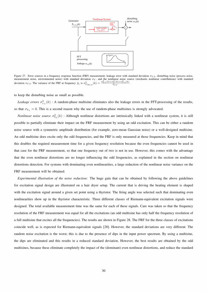
Linear system+

nonlinear

source

GBLA jw( )

noise

Generator Nonlinear System

FFTprocessing

GR jw( )

w

+

disturbingnoise

leakage

SU0U0k( )

sYL k( )

sY k( )

sYS

Figure 27. Error sources in a frequency response function (FRF) measurement: leakage error with standard deviation σY L, disturbing noise (process noise,measurement noise, environmental noise) with standard deviation σY , and the nonlinear noise source (stochastic nonlinear contributions) with standarddeviation σY S . The variance of the FRF at frequency fk is σ2

GBLA(k) =

σ2Y L(k)+σ2

Y (k)+σ2Y S(k)

SUU.

to keep the disturbing noise as small as possible.

Leakage errors σ2Y L

(k) : A random-phase multisine eliminates also the leakage errors in the FFT-processing of the results,

so that σYL = 0. This is a second reason why the use of random-phase multisines is strongly advocated.

Nonlinear noise source σ2YS

(k) : Although nonlinear distortions are intrinsically linked with a nonlinear system, it is still

possible to partially eliminate their impact on the FRF measurement by using an odd excitation. This can be either a random

noise source with a symmetric amplitude distribution (for example, zero-mean Gaussian noise) or a well-designed multisine.

An odd multisine does excite only the odd frequencies, and the FRF is only measured at those frequencies. Keep in mind that

this doubles the required measurement time for a given frequency resolution because the even frequencies cannot be used in

that case for the FRF measurement, so that one frequency out of two is not in use. However, this comes with the advantage

that the even nonlinear distortions are no longer influencing the odd frequencies, as explained in the section on nonlinear

distortions detection. For systems with dominating even nonlinearities, a large reduction of the nonlinear noise variance on the

FRF measurement will be obtained.

Experimental illustration of the noise reduction: The huge gain that can be obtained by following the above guidelines

for excitation signal design are illustrated on a hair dryer setup. The current that is driving the heating element is shaped

with the excitation signal around a given set point using a thyristor. The firing angle was selected such that dominating even

nonlinearities show up in the thyristor characteristic. Three different classes of Riemann-equivalent excitation signals were

designed. The total available measurement time was the same for each of these signals. Care was taken so that the frequency

resolution of the FRF measurement was equal for all the excitations (an odd multisine has only half the frequency resolution of

a full multisine that excites all the frequencies). The results are shown in Figure 28. The FRF for the three classes of excitations

coincide well, as is expected for Riemann-equivalent signals [28]. However, the standard deviations are very different. The

random noise excitation is the worst; this is due to the presence of dips in the input power spectrum. By using a multisine,

the dips are eliminated and this results in a reduced standard deviation. However, the best results are obtained by the odd

multisines, because these eliminate completely the impact of the (dominant) even nonlinear distortions, and reduce the standard

30

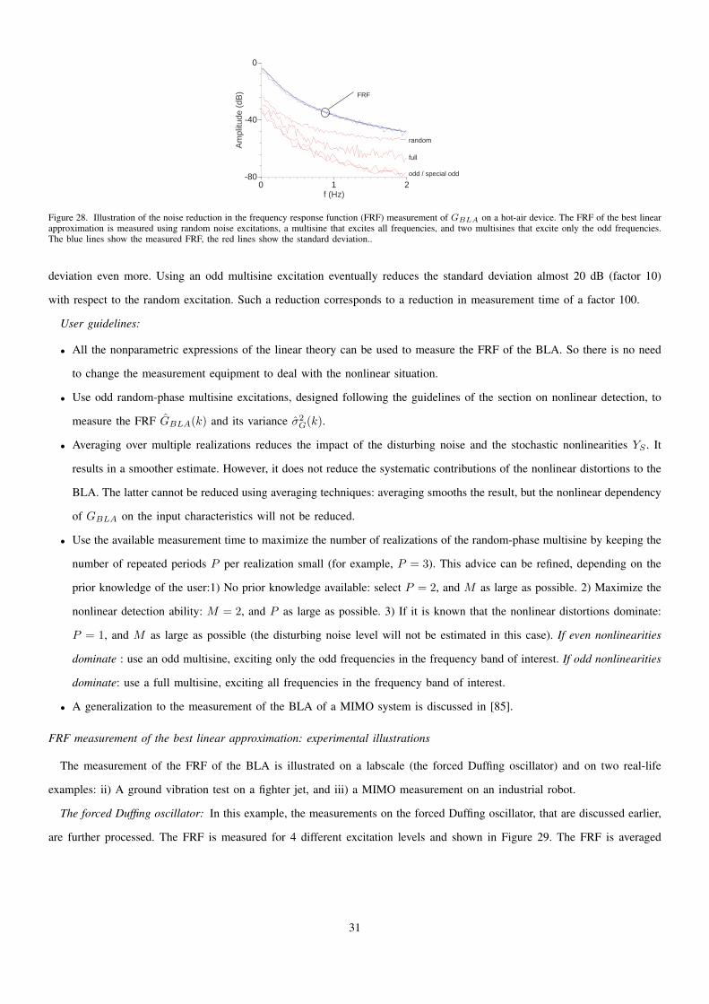
-80

-40

0

0 1 2

Am

plitu

de (

dB)

f (Hz)

FRF

random

full

odd / special odd

Figure 28. Illustration of the noise reduction in the frequency response function (FRF) measurement of GBLA on a hot-air device. The FRF of the best linearapproximation is measured using random noise excitations, a multisine that excites all frequencies, and two multisines that excite only the odd frequencies.The blue lines show the measured FRF, the red lines show the standard deviation..

deviation even more. Using an odd multisine excitation eventually reduces the standard deviation almost 20 dB (factor 10)

with respect to the random excitation. Such a reduction corresponds to a reduction in measurement time of a factor 100.

User guidelines:

• All the nonparametric expressions of the linear theory can be used to measure the FRF of the BLA. So there is no need

to change the measurement equipment to deal with the nonlinear situation.

• Use odd random-phase multisine excitations, designed following the guidelines of the section on nonlinear detection, to

measure the FRF GBLA(k) and its variance σ2G(k).

• Averaging over multiple realizations reduces the impact of the disturbing noise and the stochastic nonlinearities YS . It

results in a smoother estimate. However, it does not reduce the systematic contributions of the nonlinear distortions to the

BLA. The latter cannot be reduced using averaging techniques: averaging smooths the result, but the nonlinear dependency

of GBLA on the input characteristics will not be reduced.

• Use the available measurement time to maximize the number of realizations of the random-phase multisine by keeping the

number of repeated periods P per realization small (for example, P = 3). This advice can be refined, depending on the

prior knowledge of the user:1) No prior knowledge available: select P = 2, and M as large as possible. 2) Maximize the

nonlinear detection ability: M = 2, and P as large as possible. 3) If it is known that the nonlinear distortions dominate:

P = 1, and M as large as possible (the disturbing noise level will not be estimated in this case). If even nonlinearities

dominate : use an odd multisine, exciting only the odd frequencies in the frequency band of interest. If odd nonlinearities

dominate: use a full multisine, exciting all frequencies in the frequency band of interest.

• A generalization to the measurement of the BLA of a MIMO system is discussed in [85].

FRF measurement of the best linear approximation: experimental illustrations

The measurement of the FRF of the BLA is illustrated on a labscale (the forced Duffing oscillator) and on two real-life

examples: ii) A ground vibration test on a fighter jet, and iii) a MIMO measurement on an industrial robot.

The forced Duffing oscillator: In this example, the measurements on the forced Duffing oscillator, that are discussed earlier,

are further processed. The FRF is measured for 4 different excitation levels and shown in Figure 29. The FRF is averaged

31

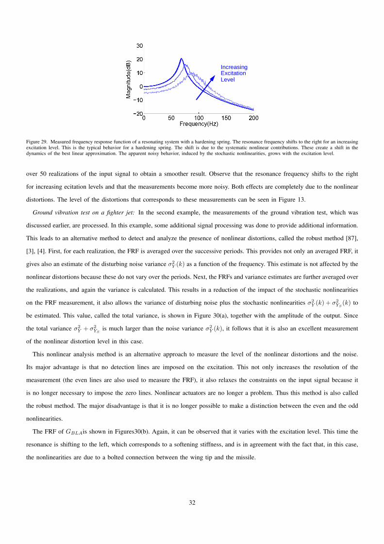
IncreasingExcitationLevel

Figure 29. Measured frequency response function of a resonating system with a hardening spring. The resonance frequency shifts to the right for an increasingexcitation level. This is the typical behavior for a hardening spring. The shift is due to the systematic nonlinear contributions. These create a shift in thedynamics of the best linear approximation. The apparent noisy behavior, induced by the stochastic nonlinearities, grows with the excitation level.

over 50 realizations of the input signal to obtain a smoother result. Observe that the resonance frequency shifts to the right

for increasing ecitation levels and that the measurements become more noisy. Both effects are completely due to the nonlinear

distortions. The level of the distortions that corresponds to these measurements can be seen in Figure 13.

Ground vibration test on a fighter jet: In the second example, the measurements of the ground vibration test, which was

discussed earlier, are processed. In this example, some additional signal processing was done to provide additional information.

This leads to an alternative method to detect and analyze the presence of nonlinear distortions, called the robust method [87],

[3], [4]. First, for each realization, the FRF is averaged over the successive periods. This provides not only an averaged FRF, it

gives also an estimate of the disturbing noise variance σ2Y (k) as a function of the frequency. This estimate is not affected by the

nonlinear distortions because these do not vary over the periods. Next, the FRFs and variance estimates are further averaged over

the realizations, and again the variance is calculated. This results in a reduction of the impact of the stochastic nonlinearities

on the FRF measurement, it also allows the variance of disturbing noise plus the stochastic nonlinearities σ2Y (k) + σ2

YS(k) to

be estimated. This value, called the total variance, is shown in Figure 30(a), together with the amplitude of the output. Since

the total variance σ2Y + σ2

YSis much larger than the noise variance σ2

Y (k), it follows that it is also an excellent measurement

of the nonlinear distortion level in this case.

This nonlinear analysis method is an alternative approach to measure the level of the nonlinear distortions and the noise.

Its major advantage is that no detection lines are imposed on the excitation. This not only increases the resolution of the

measurement (the even lines are also used to measure the FRF), it also relaxes the constraints on the input signal because it

is no longer necessary to impose the zero lines. Nonlinear actuators are no longer a problem. Thus this method is also called

the robust method. The major disadvantage is that it is no longer possible to make a distinction between the even and the odd

nonlinearities.

The FRF of GBLAis shown in Figures30(b). Again, it can be observed that it varies with the excitation level. This time the

resonance is shifting to the left, which corresponds to a softening stiffness, and is in agreement with the fact that, in this case,

the nonlinearities are due to a bolted connection between the wing tip and the missile.

32

5 10 15

-100

-50

0

Frequency (Hz)

FRF

(dB

)

(a)

7 8 9-50

-40

-30

-20

-10

Frequency (Hz)FR

F(d

B)

(b)

Figure 30. Measured frequency response function of GBLA of the F16-fighter (see Figure 16) at a small (grey line) and medium (black line) excitationlevels. A specific challenge encountered with fighter aircraft is the modeling of the wing-to-payload mounting interfaces (for example the missile on the tip ofthe wing in Figure 16(a)). For large amplitudes of vibration, friction and gaps may be triggered in these connections, resulting in a nonlinear behavior. Figure(b) shows a zoom around 7 Hz of the measurements shown in Figure (a). The levels of the total variance (red), and the disturbing noise (green) are given.Observe that the resonance frequency shifts to the left for an increasing excitation level. This corresponds to a softening spring. This behavior originates fromthe bolted connections mentioned before. In Figure (a) it is seen that the nonlinearities are largest around the resonance frequencies, and they are well abovethe disturbing noise level.

Multiple-input multiple-output FRF measurements on an industrial robot: In this example, the MIMO FRF of an industrial

robot with 6 degrees of freedom is measured (see Figure 31) [88]. The figure shows a selected set of the measured FRFs

between three motor torques and three motor accelerations. When designing excitations for MIMO measurements, additional

design aspects come into the scope besides those that were already discussed before. In a MIMO FRF measurement, a set

of linear equations with a dimension nu × nu (nu is the number of inputs) should be solved. The condition number of this

matrix affects very strongly the noise sensitivity. Using orthogonal multisine excitations [36], [85], it is possible to obtain

a condition number equal to 1, while at the same time it is still possible to make the nonlinear distortion analysis. In this

case, the total variance and the noise variance is shown. Using these signals resulted in a significant improvement of the FRF

measurements. The settings for these MIMO measurements are as follows. The measurements are averaged over 9 realizations

of an odd random-phase multisine. From each realization, a set of nu = 6 orthogonal multisines is created and is used as the

input for a single MIMO experiment. P = 2 periods are measured in steady state for each realization. The period length of

the random-phase multisine is 10 s, and 195 odd frequencies are excited in the frequency band from 1-40 Hz. The sample

frequency was fs = 2 kHz. More information can be found in [88], [89].

PARAMETRIC IDENTIFICATION OF THE BEST LINEAR APPROXIMATION

In many applications, a parametric transfer function model or state-space representation of the system is needed, together

with an estimate of the model uncertainty.

33

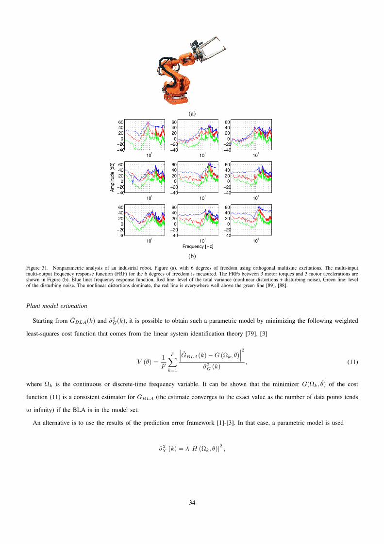
(a)

(b)

Figure 31. Nonparametric analysis of an industrial robot, Figure (a), with 6 degrees of freedom using orthogonal multisine excitations. The multi-inputmulti-output frequency response function (FRF) for the 6 degrees of freedom is measured. The FRFs between 3 motor torques and 3 motor accelerations areshown in Figure (b). Blue line: frequency response function, Red line: level of the total variance (nonlinear distortions + disturbing noise), Green line: levelof the disturbing noise. The nonlinear distortions dominate, the red line is everywhere well above the green line [89], [88].

Plant model estimation

Starting from GBLA(k) and σ2G(k), it is possible to obtain such a parametric model by minimizing the following weighted

least-squares cost function that comes from the linear system identification theory [79], [3]

V (θ) =1

F

F∑k=1

∣∣∣GBLA(k)−G (Ωk, θ)∣∣∣2

σ2G (k)

, (11)

where Ωk is the continuous or discrete-time frequency variable. It can be shown that the minimizer G(Ωk, θ) of the cost

function (11) is a consistent estimator for GBLA (the estimate converges to the exact value as the number of data points tends

to infinity) if the BLA is in the model set.

An alternative is to use the results of the prediction error framework [1]-[3]. In that case, a parametric model is used

σ2Y (k) = λ |H (Ωk, θ)|2 ,

34

and the cost function is formulated directly on the input output data leading to

Vpe (θ) =1

N

N∑t=1

(H−1(q, θ)(y(t)−G(q, θ)u(t))2.

In the general problem, the plant and noise model parameters are estimated. The reader is referred to [1], [2] to learn how to

choose the plant and noise model structure. In the motivational example, a Box-Jenkins model structure was used. In that case,

the plant and noise model have no common parameters. A simplified approach would be to put the noise model H(q, θ) = 1.

Under open-loop conditions, this will still lead to consistent estimates for GBLA, provided that GBLA is in the model set.

However, no information on the distortion levels will be available, and the uncertainty on the estimated plant model will be

larger. Under closed-loop conditions, the estimate will become also biased.

Variance estimate of the plant model

The linear system identification theory provides also a theoretical estimate of the variance of the estimated model, starting

from the assumption that the disturbing noise is independent of the excitation signal u(t). This assumption does not hold for

ys(t). As mentioned before, the stochastic nonlinearity is uncorrelated with the input, but still dependent on it. A detailed

study shows that this dependency between the input and the nonlinear distortions will lead to a much higher variance than

what is predicted by the linear theory [86].

The worst-case situation occurs for a static nonlinear system y = un, as was studied in the toy example of the previous

section. In that case, an analytical analysis can be made made for a zero-mean white Gaussian noise excitation. The BLA

y = aBLAu was given by aBLA = µn+1/µ2. The ratio between the actual variance σ2aBLA that will be observed by repeated

experiments, and the variance σ2aBLA,ind

that is obtained from the linear identification theory assuming independent noise, is

σ2aBLA

σ2aBLA,ind

= 2n+ 1.

This shows that the underestimation of the variance by the linear framework grows linearly with the nonlinear degree n. This

leads to far too optimistic uncertainty bounds; underestimation of the actual variance with a factor 7 (about 8 dB) or more

occurs.

In Figure 32, the underestimation effect is shown on the identification of a Wiener-Hammerstein system. Such a system

consists of the cascade of a linear dynamic system, a static nonlinear system, and a linear dynamic system. It can be shown,

for Gaussian excitations,

GBLA(k) = αG1(k)G2(k),

with G1, G2 the transfer functions of the first and second linear system, and α a constant that depends on the nonlinear system

and the properties of the excitation signal. From Figure 32, it can be seen that the actual observed error level in the simulations

σsim is significantly larger than the expected level σth from the linear system identification theory.

35

Wiener-Hammerstein system

Figure 32. Parametric identification of a Wiener-Hammerstein system. The theoretical σth and the actually observed σsim standard deviation are shown.

Similar results can also be observed in the experimental results in Figure 4, where it is visible that the actual variance is

about 4 dB larger than what is predicted by the linear framework.

User guidelines

• Measure the FRF GBLA(k) and its variance σ2G(k) following the guidelines for nonparametric measurements of the BLA,

and estimate the parametric model. Take care: while the uncertainty bounds of the linear theory could be safely used for

nonparametric models, they are NOT valid for the parametric model. There exists, for the time being, no simple theory

to provide better error bounds.

• The BLA can also be directly estimated from the raw input-output data in the time or frequency domain, using the classical

linear framework.

• A detailed step-by-step procedure explaining how to identify a parametric estimate of the BLA is given in Chapter 7 of

[4].

NONLINEAR DISTORTION ANALYSIS UNDER CLOSED-LOOP CONDITIONS

The nonparametric nonlinear distortion analysis method that was proposed earlier in this article has to be used under open-

loop measurement conditions. To prevent unstable behavior or saturation, the measurements on a dynamic system are often

made under closed-loop conditions. In other situations, the interaction between the system and the actuator creates closed-

loop effects, especially when the input impedance of the system is not very large with respect to the output impedance of

the actuator. Because it is the typical situation for mechanical systems, the open-loop nonlinear distortion analysis and the

concept of BLA need to be generalized to these closed-loop measurement conditions. The impact of closed-loop conditions

on the measurement of the FRF of a linear system is discussed in "Measuring the FRF of a linear system uncer closed-loop

conditions". Without special precautions, the closed-loop effect will create systematic errors on the FRF-measurement: either

36

y

C

r Gu

v

Figure 33. Measuring under feedback conditions. Observe that the input signal u(t) does not only depend on the reference signal r(t), it is also affected bythe disturbance v(t), so that the input is no longer independent of the disturbances as it is the case under open-loop measurement conditions.

the FRF of the feedforward, the FRF of the inverse feedback, or a combination of both is measured. For that reason, more

advanced measurement techniques are needed under feedback conditions.

Also the the detection and characterization of the nonlinear distortions needs to be changed. Due to the presence of a

feedback loop, the nonlinear distortions at the output of the system will also influence the input. This destroys the special input

design that was proposed and illustrated in the previous section. The input signal spectrum should be zero at the detection lines

(no excitation), but under closed-loop conditions, the nonlinear distortions will now excite these frequencies. Two strategies

are proposed to deal with this situation. First, a simple correction method is proposed and illustrated on the measurement of

the open-loop characteristics of an operational amplifier. Next, the nonlinear distortion concepts will be extended to include

more formally the closed-loop situation.

The presence of the feedback also makes it impossible to impose the specially designed multisine signals with the detection

lines put equal to zero (those frequencies that were not excited) because the feedback signal will be added to it. To deal with

that situation, two solutions are proposed. For large SNRs, a correction algorithm is proposed to compensate for the non ideal

excitation signal. Only the signals in the loop (u, y) are needed. For lower SNRs, an indirect method is proposed that requests

the availability of the reference signal r.

Characterizing nonlinear distortions under closed-loop conditions using a first-order correction

If the nonlinear distortions are not too large, and the SNR is high (for example, more than 20 dB), it can be safely assumed

that, at the excited frequencies, the reference signal dominates the disturbances, and hence, as explained in “Measuring the

FRF of a linear system under closed-loop conditions”, G ≈ G. This measured value is used to compensate for the presence

of the feedback contributions at those frequencies where the input was assumed to be zero. The direct feed through of these

disturbing terms on the output at the detection lines kdet can then be compensated for [47], [3], [4]

Ycorr(kdet) = Y (kdet)− G(kdet)U(kdet),

where G(kdet) is an interpolated value that is obtained from the neighbouring excited frequencies. At those frequencies, by

using that R(kdet) = 0, the corrected output equals

Ycorr = Y − GU =1

1 +GCV − −GC

1 +GCV = V.

37

-

+

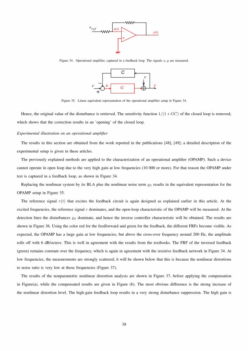
uref u t( )y t( )

Figure 34. Operational amplifier, captured in a feedback loop. The signals u, y are measured.

y

C

r Gu

v

Figure 35. Linear equivalent representation of the operational amplifier setup in Figure 34.

Hence, the original value of the disturbance is retrieved. The sensitivity function 1/(1 +GC) of the closed loop is removed,

which shows that the correction results in an ’opening’ of the closed loop.

Experimental illustration on an operational amplifier

The results in this section are obtained from the work reported in the publications [48], [49]; a detailed description of the

experimental setup is given in these articles.

The previously explained methods are applied to the characterization of an operational amplifier (OPAMP). Such a device

cannot operate in open loop due to the very high gain at low frequencies (10 000 or more). For that reason the OPAMP under

test is captured in a feedback loop, as shown in Figure 34.

Replacing the nonlinear system by its BLA plus the nonlinear noise term yS results in the equivalent representation for the

OPAMP setup in Figure 35.

The reference signal r(t) that excites the feedback circuit is again designed as explained earlier in this article. At the

excited frequencies, the reference signal r dominates, and the open-loop characteristic of the OPAMP will be measured. At the

detection lines the disturbances yS dominate, and hence the inverse controller characteristic will be obtained. The results are

shown in Figure 36. Using the color red for the feedforward and green for the feedback, the different FRFs become visible. As

expected, the OPAMP has a large gain at low frequencies, but above the cross-over frequency around 200 Hz, the amplitude

rolls off with 6 dB/octave. This is well in agreement with the results from the textbooks. The FRF of the inversed feedback

(green) remains constant over the frequency, which is again in agreement with the resistive feedback network in Figure 34. At

low frequencies, the measurements are strongly scattered; it will be shown below that this is because the nonlinear distortions

to noise ratio is very low at those frequencies (Figure 37).

The results of the nonparametric nonlinear distortion analysis are shown in Figure 37, before applying the compensation

in Figure(a), while the compensated results are given in Figure (b). The most obvious difference is the strong increase of

the nonlinear distortion level. The high-gain feedback loop results in a very strong disturbance suppression. The high gain is

38

101

102

103

104

105

−40

0

40

80

Frequency (Hz)

Am

plitu

de (

dB)

FRF

Figure 36. Nonlinear distortion analysis of an operational amplifier (OPAMP), captured in a closed-loop setup. The signals u(t), y(t) are measured. Thefeedback effects are eliminated using a compensation algorithm. A random odd excitation is used. At the excited frequencies, the open-loop frequency responsefunction FRF of the OPAMP is measured (red). At the unexcited frequencies, the inverse of the feedback loop is measured (green crosses). As expected, theOPAMP has a large gain at low frequencies, but above the crossover frequency around 200 Hz, the amplitude rolls off with 6 dB/octave. The FRF of theinverse transfer function of the feedback 1/GFB (green) remains constant over the frequency. At low frequencies the measurements are strongly scatteredbecause the nonlinear distortions to noise ratio is very low at those frequencies.

exchanged for an improved linear behavior. Without this high disturbance rejection of the feedback loop, the nonlinearities at

low frequencies would become as large as the actual output of the OPAMP. So it can be concluded that the nonlinearity level

will set the maximum gain that can be obtained with an OPAMP circuit.

Characterizing nonlinear distortions under closed-loop conditions: an extended framework

As explained before, two problems are faced to deal with measurements under closed-loop conditions: i) the FRF measurement

is biased; ii) the actual excitation signal u(t) in Figure 33 is disturbed by the nonlinear distortions that are fed back to the

input so that the detection lines are also excited, which is in conflict with their definition. In the previous sections, a simple

linear correction method was proposed to reduce the effects on the distortion analysis. Here an extended framework is shortly

presented that eliminates the bias on the FRF measurements, and generalizes the concepts of BLA and the stochastic nonlinear

contributions to closed-loop systems (the actuator, the plant, and the controller can be nonlinear). Here an intuitive explanation

is given; see [50] for a detailed and formal discussion. The basic idea is to use not only the measured input and output u, y,

but to make also explicit use of the availability of the reference signal r (see Figure 33).

The indirect FRF-measurement method: When a direct measurement of the BLA GBLA is made (16), the nonlinear distortions

YS in Y = GBLAU + Ys will create a bias

GBLA =SY USUU

= GBLA +SYSUSUU

.

(the frequency index k is dropped to simplify the notations). In general, SYSU 6= 0 because, through the feedback path, the input

U depends on the nonlinear distortions YS . The bias term SYSU/SUU can be eliminated by making an indirect measurement

of the BLA. The FRF GBLA is estimated as the division of the BLA from the reference signal to the input Gur and from the

reference to the output Gyr

GBLA,r =GyrGur

=SY RSUR

.

39

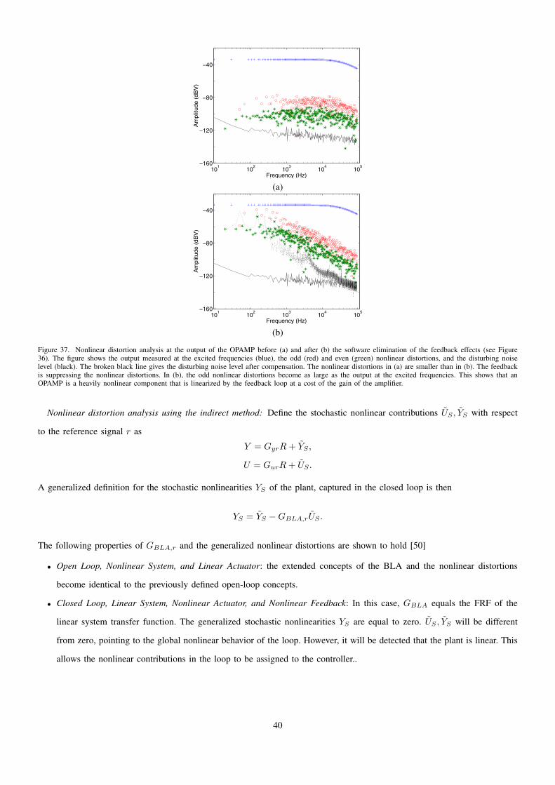
101

102

103

104

105

−160

−120

−80

−40

Output spectrum

Frequency (Hz)

Am

plitu

de (

dBV

)(a)

101

102

103

104

105

−160

−120

−80

−40

Corrected output spectrum

Frequency (Hz)

Am

plitu

de (

dBV

)

(b)

Figure 37. Nonlinear distortion analysis at the output of the OPAMP before (a) and after (b) the software elimination of the feedback effects (see Figure36). The figure shows the output measured at the excited frequencies (blue), the odd (red) and even (green) nonlinear distortions, and the disturbing noiselevel (black). The broken black line gives the disturbing noise level after compensation. The nonlinear distortions in (a) are smaller than in (b). The feedbackis suppressing the nonlinear distortions. In (b), the odd nonlinear distortions become as large as the output at the excited frequencies. This shows that anOPAMP is a heavily nonlinear component that is linearized by the feedback loop at a cost of the gain of the amplifier.

Nonlinear distortion analysis using the indirect method: Define the stochastic nonlinear contributions US , YS with respect

to the reference signal r as

Y = GyrR+ YS ,

U = GurR+ US .

A generalized definition for the stochastic nonlinearities YS of the plant, captured in the closed loop is then

YS = YS −GBLA,rUS .

The following properties of GBLA,r and the generalized nonlinear distortions are shown to hold [50]

• Open Loop, Nonlinear System, and Linear Actuator: the extended concepts of the BLA and the nonlinear distortions

become identical to the previously defined open-loop concepts.

• Closed Loop, Linear System, Nonlinear Actuator, and Nonlinear Feedback: In this case, GBLA equals the FRF of the

linear system transfer function. The generalized stochastic nonlinearities YS are equal to zero. US , YS will be different

from zero, pointing to the global nonlinear behavior of the loop. However, it will be detected that the plant is linear. This

allows the nonlinear contributions in the loop to be assigned to the controller..

40

• Closed Loop, Nonlinear System, Nonlinear Actuator, and Nonlinear Feedback: The level of the nonlinear behavior of the

plant is detected. Some precautions should be taken when interpreting the presence of even and odd nonlinear contributions.

Precise conditions, that can be easily verified in practice, are given in [50], to check if the results are reliable.

These results confirm that the simplified procedure that was explained earlier in this article can be used safely if the SNR is

more than 10 dB (bias below 10%) or 20 dB (bias below 1%).

PUBLICLY AVAILABLE SOFTWARE

All the results in this article can be reproduced using publicly available Matlab toolboxes. The motivational example was

produced using the System Identification toolbox of Matlab (Mathworks). Alternatively, the freely available frequency-domain

identification toolbox FDIDENT could be used to obtain similar results (http://home.mit.bme.hu/~kollar/fdident/). This toolbox

also includes the tools to design the random-phase multisines and to perform the nonparametric nonlinear analysis. In [4],

all the procedures that are presented in this article are discussed in full detail, and the related Matlab software can be freely

downloaded at (booksupport.wiley.com).

CONCLUSIONS

This article studied the problem of how to deal with nonlinear distortions in the linear system identification framework. In a

first step, nonparametric tools were discussed to detect the presence and the level of the nonlinear distortions, and to analyze

their nature (even or odd). Next, the concept of the BLA was introduced. The dependency of the BLA on the user choices

was studied (choice of the excitation signal, and choice of the approximation criterion). Optimal measurement strategies to

measure the FRF of the BLA were presented, and eventually the impact of the nonlinear distortions on the linear parametric

identification approach were discussed. All these methods were illustrated on real-life examples.

ACKNOWLEDGEMENT

This work was supported in part by the Fund for Scientific Research (FWO-Vlaanderen), by the Flemish Government

(Methusalem), the Belgian Government through the Inter-university Poles of Attraction (IAP VII) Program, and by the

ERC advanced grant SNLSID, under contract 320378. The authors thank Chris Criens, Technical University Eindhoven,

The Netherlands, for the contribution on the Section “Characterization of the air path of a diesel engine”, including Figures

14 and 15; P.W.M.J. Nuij, Technical University Eindhoven, The Netherlands, for the contribution to the Section “Higher-

order sinusoidal input describing functions”, including Figures 17 and 18; E. Wernholt, Linkoping University, Sweden, for the

contribution to the Section “Multiple-input multiple-output FRF measurements on an industrial robot”, including the Figure

31; G. Kerschen and J.P. Noel, Univeristï¿œ de Liï¿œge, Belgium, for the Sections “Swept sine test”, including Figures 19 and

20, and “Ground vibration test on an air fighter”, including Figures 16 and 30; B. Peeters, LMS International, part of Siemens

Product Lifecycle Management, Belgium, for the contributions to the “Ground vibration test on an air fighter”, including

Figures 16 and 30.

41

SIDEBAR 1: A MATHEMATICAL FRAMEWORK FOR NONLINEAR SYSTEMS

In this section, some basic results of the Volterra theory [18] are given, without proof, to provide the reader with an intuitive

insight into the behavior of nonlinear systems. The emphasis will be to show how a nonlinear system is shifting the input

power from one frequency to the other. Three intermediate steps will be made:

• From a one-dimensional impulse response (linear theory) to a multidimensional impulse response (nonlinear system).

• multidimensional frequency description of nonlinear systems: a tool for intuitive insight in nonlinear behavior [26], [70].

• Return to the physical world: collapsing the multidimensional frequency description to a single dimension.

Using Volterra kernels as multidimensional impulse responses

A linear system is characterized by its impulse response g(t), and the input-output relation is given by the convolution

integral

y(t) =

∫ ∞0

g(τ)u(t− τ)dτ.

In the Volterra approach, the output of the nonlinear system is given by the sum of the contributions of increasing nonlinear

degree α

y(t) =

∞∑α=1

yα(t), (12)

with yα(t) =∫∞0. . .∫∞0gα(τ1, . . . , τα)u(t − τ1) . . . u(t − τα)dτ1 . . . dτα. The kernel gα(τ1, . . . , τα) is the multidimensional

impulse response of degree α.

Multidimensional frequency response functions

The signal yα(t) in (12) can be generalized to a multidimensional time signal yα(t1, . . . , tα) =∫∞0. . .∫∞0gα(τ1, . . . , τα)u(t1−

τ1) . . . u(tα−τα)dτ1 . . . dτα. The original signal is retrieved by putting t1 = . . . = tα = t. The multidimensional representation

in the frequency domain becomes

Y α(ω1, . . . , ωα) = Gα(ω1, . . . , ωα)U(ω1) . . . U(ωα), (13)

with Gα(ω1, . . . , ωα) the multidimensional Fourier transform of gα(τ1, . . . , τα). This multidimensional representation in the

frequency domain is very similar to the result for the linear case: the output spectrum is obtained as the (multidimensional)

product of the transfer function with the input.

From a multidimensional to a one-dimensional frequency variable

The one-dimensional spectrum Y α(ω) is retrieved by looking for all frequency combinations ω1, . . . , ωα, such that ω1 +

. . .+ωα = ω. These are retrieved by Y α(ω) =∫∞−∞ . . .

∫∞−∞ Y α(ω1, . . . , ωα−1, ω−ω1 + . . .+ωα−1)dω1 . . . dωα−1. Observe

that this is a generalization of the response of a nonlinear system to a sinusoid.

42

Measuring the Volterra kernels

Although the Volterra representation is an attractive nonparametric description of a general class of nonlinear systems, there

are only a few methods described in the literature to measure the Volterra kernels, most of them focussing on systems with

short memories. The major reason for this lack of interest is the exploding number of parameters to be identified due to the

multidimensional nature of the kernels. A first possibility is to use higher-order correlation methods [18], often combined

with an orthogonal representation of the Volterra series, for example, using a Wiener representation. Methods were presented

to avoid the long correlation times that are needed by the use of well-designed excitation signals [73]. The basic idea is to

generate a multisine where the active frequencies are selected such that the harmonic interference of the kernels of different

degree is eliminated up to a given degree (for example, degree 4). The design of such ’no interharmonic distortion’ signals

(NID-signals) is discussed in detail in [71], [72]. Methods to measure the multivariate FRF that make use of such signals are

discussed, for example, in [73], [74].

SIDEBAR 2: THE BEST LINEAR APPROXIMATION OF A VOLTERRA SYSTEM

In this section, an explicit expression is given for the BLA for a Volterra kernel of degree α. The multidimensional output

is given in (13). For a multisine excitation, the contributions at a given frequency k are retrieved by looking for all frequency

combinations such that∑αi=1 ki = k, with ki an excited frequency, see also (1). These multivariate output contributions are

given by

Y (k1, k2, . . . , kα) = Gα(k1, k2, . . . , kα)U(k1)U(k2) . . . U(kα), (14)

for a kernel of degree α. Among these, only the contributions for which

U(k1)U(k2) . . . U(kα)U(−k) = U(k1)U(k2) . . . U(kα)U(k), (15)

(where the overbar denotes the complex conjugate) do not depend on the input phases ∠U will contribute to the BLA. If this

product would still depend on the random-phases of the input, its expected value over multiple realizations would be zero

because, by definition, for a random-phase multisine Eejϕ = 0, and the phases of a random-phase multisine are independent

over the frequency. So it should be possible to write (15) as a real number, which can only be done if all the components U

in this product can be combined in pairs of complex-conjugated inputs, for example U(ki)U(−ki) = |U(ki)|2, such that the

input phases are cancelled.

From this result, it can be seen that only kernels with an odd degree α can contribute. For the odd kernels, the contribution

of degree α = 2β + 1 to YBLA(k) is

YBLA(k) =∑k1

. . .∑kβ

Ck,k1,−k1,...,kβ ,−kβGα(k, k1,−k1, . . . , kβ ,−kβ)|U(k1)|2 . . . |U(kβ)|2U(k),

where the sum runs over all frequencies that are excited. The constant Ck,k1,−k1,...,kβ ,−kβ accounts for the number of all

possible frequency combinations that are obtained by changing the position of the frequencies in Gα(k, k1,−k1, . . . , kβ ,−kβ).

43

yuR Sf

Figure 38. Wiener-Hammerstein system. A static nonlinear system f is sandwiched between the linear dynamic systems R,S.

Example: a Wiener-Hammerstein system

Consider the Wiener-Hammerstein system in Figure 38 excited by a random-phase multisine with F excited frequencies.

For a static nonlinearity f = x3, the multivariate output (14) becomes

Y (k1, k2, k3) = Gα(k1, k2, k3)U(k1)U(k2)U(k3).

For the Wiener-Hammerstein system, this reduces further to

Y (k1, k2, k3) = S(k1 + k2 + k3)R(k1)R(k2)R(k3)U(k1)U(k2) . . . U(k3).

The contributions YBLA(k) are then given by looking for all combinations k = k1 + k2 + k3 that depend only on the phase

of U(k)

YBLA(k) = U(k)× 6S(k)R(k)

F∑l=1

|S(l)|2|U(l)|2 − EY ,

with EY = 3S(k)R(k)|S(k)|2|U(k)|2U(k) a correction term because for l = k, only 3 permutations are possible instead of

6 [83].

The stochastic nonlinear contributions YS(k) are given by all other terms where condition (15) does not hold, for example,

the contribution S(k)R(k − 1)R(−k − 2)R(k + 3)U(k − 1)U(−k − 2)U(k + 3).

SIDEBAR 3: MEASURING THE FRF OF A LINEAR SYSTEM UNDER CLOSED-LOOP CONDITIONS

Measuring the FRF of a system under closed-loop conditions requires special precautions. Depending on the SNR of the

measurements, either the FRF of the feedforward branch, the inverse feedback branch, or a combination of both results. The

most simple approach to measure the FRF of a system is to measure the input and output signals u(kTs), y(kTs), k = 1, . . . , N ,

with Ts = 1/fs the sampling period, calculate the discrete Fourier transforms U(k), Y (k) of these signals, and divide the

resulting spectra to obtain an estimate G(k) = Y (k)/U(k) at the frequency kfs/N . The raw data need to be averaged to

reduce the noise and leakage errors. This should be done before dividing the spectra, because large errors will occur at

those frequencies where U(k) becomes very small. For that reason, it is better to estimate first the cross- and auto-spectrum

SY U , SUU , and the FRF estimate at frequency k is

G(k) =SY U (k)

SUU (k). (16)

These methods became popular in the 1960s, especially in the combination with pseudo random-binary excitation signals to

generate multifrequency excitations [42]-[45]. To do so, the record is split in P subrecords, and for each of these the discrete

44

Fourier transform U [l](k), Y [l](k), l = 1, . . . , P is calculated. The cross- and auto-power spectrum estimate is then obtained

[4]

SY U (k) =1

P

P∑l=1

Y [l](k)U [l](k), SUU (k) =1

P

P∑l=1

|U [l](k)|2,

where U is the complex conjugate of U. When the measurement is made under feedback conditions (see Figure 33), the output

y(t) depends on both the measured input u(t) and the disturbance source v(t). Due to the presence of the feedback loop, the

signal u depends also on the disturbance v. As a result, the FRF measurement at frequency k converges to [46]

G =GSRR − CSV VSRR + |C|2SV V

.

This expression reduces to G = G, if SV V = 0 (r dominates over v), and G = −1C , if SRR = 0 (v dominates over r). For

mixed SNR, the estimate becomes a mixture of the feedforward and feedback characteristics.

REFERENCES

[1] L. Ljung. System Identification: Theory for the User (second edition). Prentice Hall, Upper Saddle River, New Jersey, 1999.

[2] T. Sï¿œderstrï¿œm, and P. Stoica. System Identification. Prentice-Hall, Englewood Cliffs, 1989.

[3] R. Pintelon, and J. Schoukens. System Identification. A Frequency Domain Approach, 2nd edition. Wiley-IEEE-press, Piscataway, 2012.

[4] J. Schoukens, R. Pintelon, Y. Rolain. Mastering System Identification in 100 Exercises. Wiley-IEEE-press, Piscataway, 2012.

[5] D.J. Ewins. Modal Testing: Theory, Practice and Application. Research Studies Press LTD, Hertfordshire, 2000.

[6] T. Oomen, R. van Herpen, S. Quist, M. van de Wal, O. Bosgra, M. Steinbuch, “Connecting system identification and robust control for

next-generation motion control of a wafer stage,” IEEE Trans. on Control Systems Technology, vol. 22, pp. 102-118, 2014.

[7] J. Verbeeck, R. Pintelon, P. Lataire, “Identification of synchronous machine parameters using a multiple input multiple output approach,” IEEE

Trans. on Energy Conversion, vol. 14, pp. 909-917, 1999.

[8] J. Verbeeck, R. Pintelon, P. Lataire, “Infulence of saturation on estimated synchronous machine parameters in standstill frequency response

tests,” IEEE Trans. on Energy Conversion, vol. 15, pp. 277-283, 2000.

[9] N. Dedene, R. Pintelon, P. Lataire, “Measurement of multivariable frequency response functions in the presence of nonlinear distortions - Some

practical aspects,” IEEE Trans. on Instrumentation and Measurement, vol. 31, pp. 577-582, 2002.

[10] N. Dedene, R. Pintelon, P. Lataire, “Estimation of a global synchronous machine model using a multiple-input multiple-output estimator,” IEEE

Trans. on Energy Conversion, vol. 18, pp. 11-16, 2003.

[11] D.E. Rivera, H. Lee, H.D. Mittelmann, M.W. Braun, “Constrained multisine input signals for plant-friendly identification of chemical process

systems,” Journal of Process Control, vol. 19, pp. 623-635, 2009.

[12] B. Peeters, C.E. Ventura, “Comparative study of modal analysis techniques for bridge dynamic characteristics,” Mechanical Systems and Signal

Processing, vol. 17, pp. 965-988, 2003.

[13] D.T. Westwick, and R.E. Kearney. Identification of Nonlinear Physiological Systems. IEEE-Wiley, 2003.

[14] S.A. Billings. Nonlinear system identification : NARMAX methods in the time, frequency, and spatio-temporal domains. John Wiley & Sons Ltd,

2013.

[15] S.A. Billings, and S.Y. Fakhouri, “Identification of systems containing linear dynamic and static nonlinear elements,” Automatica, 18, pp. 15-26,

1982.

[16] G. Kerschen, K. Worden, A.F. Vakakis, J. Golinval, “Past, present and future of nonlinear systems identification in structural dynamics,”

Mechanical Systems and Signal Processing, vol. 20, pp. 505-592, 2006.

[17] F. Giri, and E.W. Bai (Eds.). Block-oriented Nonlinear System Identification. Springer, 2010.

45

[18] M. Schetzen. The Volterra and Wiener Theories of Nonlinear Systems. Wiley and Sons, New York, 2006.

[19] O. Nelles. Nonlinear System Identification. Springer, 2001.

[20] R. Haber and L. Kevicky. Nonlinear System Identification - Input-Output Modeling Approach. Volume 1&2. Kluwer Academic Publishers, 1999.

[21] J. Paduart, L. Lauwers, J. Swevers, K. Smolders, J. Schoukens, and R. Pintelon, “Identification of nonlinear systems using polynomial nonlinear

state space models,” Automatica, 46., pp. 647-656, 2010.

[22] J. Schoukens, “System identification in a real world,” The 13th International workshop on Advanced Motion Control AMC2014, Yokohama,

Japan, March 14-16, 2014.

[23] J.M.T. Thompson and H.B. Stewart. Nonlinear Dynamics and Chaos. Wiley, New York (1986).

[24] Y. Ueda, “Survey of Regular and Chaotic Phenomena in the forced Duffing Oscillator,” Chaos, Solutions & Fractals, vol. 1, pp. 199-231, 1991.

[25] U. Forssell and L. Ljung, “A projection method for closed-loop identification,” IEEE Trans. on Automatic Control, vol. 45, pp. 2101-2106, 2000.

[26] L.O. Chua and C.-Y. Ng, “Frequence domain analysis of nonlinear systems: General theory,” IEE Electron. Circuits Syst., 3, pp. 165-185, 1979.

[27] S. Boyd and L.O. Chua, “Fading Memory and the Problem of Approximating Nonlinear Operators with Volterra Series,” IEEE Trans. on Circuits

and Systems, 32, pp. 1150-1161, 1985.

[28] J. Schoukens, J. Lataire, R. Pintelon, and G. Vandersteen, “Robustness issues of the equivalent linear representation of a nonlinear system,”

IEEE Trans. Instrum. Meas., vol. 58, pp. 1737-1745, 2009.

[29] J. Schoukens, R. Pintelon, E. van der Ouderaa, and J. Renneboog, “Survey of excitation signals for FFT based signal analyzers,” IEEE Trans.

on Instrum. and Meas., vol. 37, pp. 343-352, 1988.

[30] P. Guillaume, J. Schoukens, R. Pintelon, and I. Kollar, “Crest-factor minimization using nonlinear Chebyshev approximation methods,” IEEE

Trans. on Instrum. and Meas., vol. 40, 982-989, 2002.

[31] A.H. Tan, and K.R. Godrey, “The generation of binary and near-binary pseudorandom signals: an overview,” IEEE Trans. on Instrum. and Meas.,

vol. 51, pp. 583-588, 2002.

[32] H.K. Wong, J. Schoukens, K.R. Godfrey, “Analysis of Best Linear Approximation of a Wiener-Hammerstein System for Arbitrary Amplitude

Distributions,” IEEE Trans. on Instrum. and Meas., vol. 61, pp. 645-654, 2012.

[33] H.K. Wong, J. Schoukens, K.R. Godfrey, “Design of Multilevel Signals for Identifying the Best Linear Approximation of Nonlinear Systems,”

IEEE Trans. on Instrum. and Meas., vol. 62, pp. 519-524, 2013.

[34] E. Geerardyn, Y. Rolain, J. Schoukens, “Design of quasi-logarithmic multisine excitations for robust broad frequency band measurements,” IEEE

Trans. Instrum. Meas., vol. 62, pp. 1364-1372, 2013.

[35] R. Pintelon, K. Barbï¿œ, G. Vandersteen, J. Schoukens, “Improved (non-)parametric identification of dynamic systems excited by periodic

signals,” Mechanical Systems and Signal Processing, vol. 25, pp. 2683-2704, 2011.

[36] R. Pintelon, G. Vandersteen, J. Schoukens, Y. Rolain, “Improved (non-)parametric identification of dynamic systems excited by periodic

signals—The multivariate case,” Mechanical Systems and Signal Processing, vol. 25, pp. 2892-2922, 2011.

[37] A. Marconato, M. Schoukens, Y. Rolain and J. Schoukens, “Study of the effective number of parameters in nonlinear identification benchmarks,”

52nd IEEE Conference on Decision and Control, December 10-13, 2013, Florence, Italy.

[38] C. Criens. Air-path control of clean diesel engines : for disturbance rejection on NOx, PM and fuel efficiency. PhD-thesis, TUEindhoven, 2014.

[39] C. Criens, T. Van Keulen, F. Willems, M. Steinbuch. A Control Oriented Multivariable Identification Procedure for Turbocharged Diesel Engines.

International Journal of Powertrains, In Press.

[40] C. H.A. Criens, F.P.T. Willems, T.A.C. van Keulen, and M. Steinbuch, “Disturbance rejection in diesel engines for low emissions and high fuel

efficiency,” IEEE Trans. on Control Systems Technology, vol. 23, 662-669, 2015.

[41] Y. Govers, M. Bï¿œswald, P. Lubrina, S. Giclais, C. Stephan, N. Botargues, “Airbus A350XWB ground vibration testing: efficient techniques

for customer oriented on-site modal identification,” International Conference on Noise and Vibration Engineering ISMA2014, Leuven, Belgium,

pp. 2495-2507, 2014.

[42] J.S. Bendat and A.G. Piersol. Random Data: Analysis and Measurement Procedures, Wiley, 2010.

[43] A.D.G. Hazlerigg, and A.R.M. Noton, “Application of crosscorrelating equipment to linear-system identification,” Proceedings IEE, vol. 112,

2385-2400, 1965.

46

[44] K.R. Godfrey, “The Theory of the Correlation Method of Dynamic Analysis and its Application to Industrial Processes and Nuclear Power

Plant,” Measurement and Control, vol. 2, pp. 65-72, 1969.

[45] P.E. Wellstead, “Non-Parametric Methods of System Identification,” Automatica, vol. 17, pp. 55-69, 1981.

[46] P.E. Wellstead, “Reference Signals for Closed-Loop Identification,” International Journal of Control, vol. 26, pp. 945-962, 1977.

[47] K. Vanhoenacker, and J. Schoukens, “Detection of nonlinear distortions with multisine excitations in the case of nonideal behavior of the input

signal,” IEEE Trans. on Instrumentation and Measurement, vol. 52, pp. 748-753, 2003.

[48] R. Pintelon, G. Vandersteen, L. De Locht, Y. Rolain, and J. Schoukens, “Experimental characterization of operational amplifiers: A system

identification approach - Part I: Theory and simulations,” IEEE Trans. on Instrumentation and Measurement, vol. 53, pp. 854-862, 2004.

[49] R. Pintelon, Y. Rolain, G. Vandersteen, and J. Schoukens, “Experimental characterization of operational amplifiers: A system identification

approach - Part II: Calibration and measurements,” IEEE Trans. on Instrumentation and Measurement, vol. 53, pp. 863-876, 2004.

[50] R. Pintelon, and J. Schoukens, “FRF measurement in nonlinear systems operating in closed loop,” IEEE Trans. on Instrum. and Meas., vol. 62,

pp. 1334-1345, 2013.

[51] K. Vanhoenacker, J. Schoukens, J. Swevers, and D. Vaes, “Summary and comparing overview of techniques for the detection of non-linear

distortions,” International Conference on Noise and Vibration Engineering ISMA2002, Leuven, Belgium, pp. 1241-1255, 2002.

[52] K. Vanhoenacker. Frequency Response Function Measurements in the Presence of Non-Linear Distortions. PhD thesis, Vrije Universiteit Brussel,

Belgium, 2003.

[53] K. Worden, and G.R. Tomlinson. Non-linearity in Structural Dynamics, Detection, Identification and Modelling. Institute of Physics Publisching

Ltd, London, England, 2001.

[54] J.M.M. Silva, and N.M.M. Maia. Theoretical and Experimental Modal Analysis. Research Studies Press LTD, Taunton, England, 1997.

[55] D. Choi, J.H. Chang, R.O. Stearman, and E.J. Powers, “Bispectral identification of nonlinear mode interactions,” Proceedings of the 2nd

International Modal Analysis Conference, Florida, U.S., pp 602-609, 1984.

[56] J.H. Chang, R.O. Stearman, D. Choi and E.J. Powers, “Identification of aero elastic phenomenon employing bispectral analysis techniques,”

Proceedings of the 3rd International Modal Analysis Conference, Orlando, Florida (U.S.), pp. 956-964, 1985.

[57] G.R. Tomlinson, “Developments in the use of the Hilbert transform for detecting and qualifying nonlinearities associated with frequency response

function measurements,” Mechanical Systems and Signal Processing, vol. 1, pp. 151-171, 1987.

[58] M. Enqvist, J. Schoukens, R.Pintelon, “Detection of unmodeled nonlinearities using correlation methods,” IEEE Instrumentation and Measurement

Technology Conference, IMTC 2007, Warsaw, Poland, 2007.

[59] A.S. McCormack, K.R. Godfrey, and J.O. Flower, “The detection of an compensation for nonlinear effects using periodic input signals,” Control

94, Warwick (UK), pp. 297-302, 1994.

[60] A. Gelb, and W. E. Vander Velde. Multiple-Input Describing Functions and Nonlinear System Design. McGraw Hill, 1968

[61] P.W.J.M. Nuij, O.H. Bosgra, and M. Steinbuch, “Higher-order sinusoidal input describing functions for the analysis of non-linear systems with

harmonic responses,” Mechanical Systems and Signal Processing, vol. 20, pp. 1883-1904, 2006.

[62] P.W.J.M. Nuij, M. Steinbuch, and O.H. Bosgra, “Measuring the higher order sinusoidal input describing functions of a nonlinear-plant operating

in feedback,” Control Engineering Practice, vol. 16, pp. 101-113, 2008.

[63] P.W.J.M. Nuij, M. Steinbuch, and O.H. Bosgra, “Experimental characterization of the stick/sliding transition in a precision mechanical system

using the third order sinusoidal input describing function,” Mechatronics, vol. 18, pp. 100-100, 2008.

[64] J.P. Noï¿œl, L. Renson, and G. Kerschen, “Complex dynamics of a nonlinear aerospace structure: Experimental identification and modal

interactions,” Journal of Sound and Vibration, vol. 333, pp. 2588-2607, 2014.

[65] European Cooperation for Space Standardization. Space engineering testing ECSS-E-ST-10-03C. ESA ESTEC, 2012.

[66] N. Roy, and A. Girard, “Revisiting the effect of sine sweep rate on modal identification”. 12th European Conference on Space Structures,

Materials & Environmental Testing, Noordwijk, The Netherlands, 2012.

[67] G. Gloth, and M. Sinapius (2004). “Analysis of swept-sine runs during modal identification”, Mechanical Systems and Signal Processing, pp.

1421-1441, 2004.

47

[68] R. Pintelon, J. Schoukens, G. Vandersteen, and K. Barbe, “Estimation of nonparametric noise and FRF models for multivariable systems-Part

I: Theory,” Mechanical Systems and Signal Processing, 24, pp. 573-595, 2010.

[69] W.D. Widanage, J. Stoev, A. Van Mulders, J. Schoukens, G. Pinte, “Nonlinear system-identification of the filling phase of a wet-clutch system,”

Control Engineering Practice, 19, pp.1506-1516, 2011.

[70] L.O. Chua, and C.Y.Ng, “Frequency domain analysis of nonlinear systems: formulation of transfer functions,” IEE Electronic Circuits and

Systems, vol. 3, pp. 165-185, 1979.

[71] C. Evans, D. Rees, and L. Jones, “Nonlinear disturbance errors in sustem identification using multisine test signals,” IEEE Trans. on Instrum.

and Meas., vol. 43, pp. 238-244, 1944.

[72] C. Evans, D. Rees, L. Jones, and M. Weis, “Periodic signals for measuring nonlinear Volterra kernels,” IEEE Trans. on Instrum Meas., vol. 45,

pp. 362-371, 1996.

[73] S. Boyd, Y.S. Tang, and L.O. Chua, “Measuring Volterra Kernels,” IEEE Trans. on Circuits and Systems, vol. 30, pp. 571-577, 1983.

[74] A.H. Tan, and K. Godfrey, “Identification of Wiener-Hammerstein models using linear interpolation in the frequency domain (LIFRED),” IEEE

Trans. on Instrum. and Meas., vol. 51, pp. 509-521, 2002.

[75] M. Enqvist. Linear Models of Nonlinear systems. PhD Thesis No. 985, Institute of technology, Linkï¿œping University, Sweden, 2005.

[76] M. Enqvist, and L. Ljung, “Linear approximations of nonlinear FIR systems for separable input processes,” Automatica, 41, vol. 7, 459-473,

2005.

[77] P.M. Mï¿œkilï¿œ, and J.R. Partington, “Least-squares LTI approximation of nonlinear systems and quasistationarity analysis,” Automatica 40,

vol. 7, pp. 1157-1169, 2004.

[78] J.J. Bussgang. Cross-correlation functions of amplitude-distorted Gaussian signals. Technical Report, 216, MIT Laboratory of Electronics, 1952.

[79] J. Schoukens, T. Dobrowiecki, and R. Pintelon, “Parametric and nonparametric identification of linear systems in the presence of nonlinear

distortions. A frequency domain approach,” IEEE Trans. Autom. Contr., 43, vol. 2, 176-190, 1998.

[80] J. Schoukens, R. Pintelon, T. Dobroviecki, and Y. Rolain, “Identification of linear systems with nonlinear distortions,” Automatica, 41, pp.

491-504, 2005.

[81] J. Schoukens, T. Dobrowiecki, Y. Rolain, and R. Pintelon, “Upper Bounding Variations of Best Linear Approximations of Nonlinear Systems

in Power Sweep Measurements,” IEEE Trans. on Instrum. and Meas., vol. 59, pp. 1141-1148, 2010.

[82] J. Schoukens, Y. Rolain, R. Pintelon, and T. Dobrowiecki, “Analysis of windowing/leakage effects in frequency response function measurements,”

Automatica 42, vol. 1, 27-38, 2006.

[83] C. Evans, and D. Rees, “Nonlinear distortions and multisine signals - Part I: Measuring the best linear approximation,” IEEE Trans. on Instrum.

and Meas., vol. 49, pp. 602-609, 2000.

[84] J. Schoukens, K. Barbï¿œ, L. Vanbeylen and R. Pintelon, “Nonlinear Induced Variance of Frequency Response Function Measurements,” IEEE

Trans. on Instrum. and Meas., 59, pp. 2468-2474, 2010.

[85] T. Dobrowiecki, and J. Schoukens, “Measuring a linear approximation to weakly nonlinear MIMO systems,” Automatica, vol. 43 (10), 1737-1751,

2007.

[86] J. Schoukens and R. Pintelon, “Study of the Variance of Parametric Estimates of the Best Linear Approximation of Nonlinear Systems,” IEEE

Trans. on Instrum. and Meas., 59, pp. 3156-3167, 2010.

[87] T. D’Haene, R. Pintelon, J. Schoukens, and E. Van Gheem, “Variance analysis of frequency response function measurements using periodic

excitations,” IEEE Trans. Instrum. Meas., vol. 54, pp. 1452-1456, 2005.

[88] E. Wernholt and S. Gunnarsson, “Estimation of Nonlinear Effects in Frequency Domain Identification of Industrial Robots,” IEEE Trans. on

Instrum. and Meas., vol. 57, pp. 856-863, 2008.

[89] E. Wernholt. Multivariable Frequency-Domain Identification of Industrial Robots. Linkï¿œping Studies in Science and Technology. Dissertations.

No. 1138, Linkï¿œping University, 2007.

Biographies

Johan Schoukens received both the Master’s degree in electrical engineering in 1980, and the PhD degree in engineering

48

sciences in 1985 from the Vrije Universiteit Brussel (VUB), Brussels, Belgium. In 1991 he received the degree of Geaggregeerde

voor het Hoger Onderwijs from the VUB, and in 2014 the degree of Doctor of Science from The University of Warwick. From

1981 to 2000, he was a researcher of the Belgian National Fund for Scientific Research (FWO-Vlaanderen) at the Electrical

Engineering Department of the VUB where he is currently a full-time professor in electrical engineering. Since 2009, he is

visiting professor at the department of Computer Sciences of the Katholieke Universiteit Leuven. His main research interests

include system identification, signal processing, and measurement techniques. He has been a Fellow of IEEE since 1997. He

was the recipient of the 2002 Andrew R. Chi Best Paper Award of the IEEE Transactions on Instrumentation and Measurement,

the 2002 Society Distinguished Service Award from the IEEE Instrumentation and Measurement Society, and the 2007 Belgian

Francqui Chair at the Universitￜ Libre de Bruxelles (Belgium). Since 2010, he is a member of Royal Flemish Academy

of Belgium for Sciences and the Arts. In 2011 he received a Doctor Honoris Causa degree from the Budapest University of

Technology and Economics (Hungary). Since 2013, he is an honorary professor of the University of Warwick.

Mark Vaes graduated as an Industrial Engineer in Electromechanics at the Erasmushogeschool Brussel. In February 2013

he joined the ELEC department as a PhD student. His main interests are in the field of system identification of linear and

nonlinear systems.

Rik Pintelon received a Master’s degree in electrical engineering in 1982, a doctorate (PhD) in engineering in 1988, and

the qualification to teach at university level (geaggregeerde voor het hoger onderwijs) in 1994, all from the Vrije Universiteit

Brussel (VUB), Brussels, Belgium. In 2014 he received the degree of Doctor of Science (DSc) from the University of Warwick

(UK) for publications with the collective title “Frequency Domain System Identification: A Mature Modeling Tool”. From 1982

to 1984 and 1986 to 2000, he was a researcher with the Belgian National Fund for Scientific Research (FWO-Vlaanderen) at

the Electrical Engineering (ELEC) Department of the VUB. From 1984 to 1986 he did his military service overseas in Tunesia

at the Institut National Agronomique de Tunis. From 1991 to 2000 he was a part-time lecturer at the VUB, and since 2000 he

is a full-time professor in electrical engineering at the same department. Since 2009, he is visiting professor at the department

of Computer Sciences of the Katholieke Universiteit Leuven, and since 2013 he is an honorary professor in the School of

Engineering of the University of Warwick. His main research interests include system identification, signal processing, and

measurement techniques. He is the coauthor of 4 books on system identification and the coauthor of more than 200 articles in

refereed international journals. He has been a Fellow of IEEE since 1998 and was the recipient of the 2012 IEEE Joseph F.

Keithley Award in Instrumentation and Measurement (IEEE Technical Field Award).

49