IEEE TRANSACTIONS ON EVOLUTIONARY COMPUTATION…jbongard/papers/2004_EC_Bongard.pdf · Nonlinear...

IEEE TRANSACTIONS ON EVOLUTIONARY COMPUTATION, VOL. 9, NO. 4, AUGUST 2005 361

Nonlinear System Identification UsingCoevolution of Models and Tests

Josh C. Bongard and Hod Lipson

Abstract—We present a coevolutionary algorithm for inferringthe topology and parameters of a wide range of hidden nonlinearsystems with a minimum of experimentation on the target system.The algorithm synthesizes an explicit model directly from theobserved data produced by intelligently generated tests. Thealgorithm is composed of two coevolving populations. One popu-lation evolves candidate models that estimate the structure of thehidden system. The second population evolves informative teststhat either extract new information from the hidden system orelicit desirable behavior from it. The fitness of candidate modelsis their ability to explain behavior of the target system observed inresponse to all tests carried out so far; the fitness of candidate testsis their ability to make the models disagree in their predictions. Wedemonstrate the generality of this estimation-exploration algorithmby applying it to four different problems—grammar induction,gene network inference, evolutionary robotics, and robot damagerecovery—and discuss how it overcomes several of the pathologiescommonly found in other coevolutionary algorithms. We showthat the algorithm is able to successfully infer and/or manipulatehighly nonlinear hidden systems using very few tests, and that thebenefit of this approach increases as the hidden systems possessmore degrees of freedom, or become more biased or unobservable.The algorithm provides a systematic method for posing synthesisor analysis tasks to a coevolutionary system.

Index Terms—Coevolution, evolutionary robotics, gene networkinference, grammar induction, nonlinear topological system iden-tification.

I. INTRODUCTION

SYSTEM identification is a ubiquitous tool in both scienceand engineering. Given some partially hidden system, the

experimenter applies a series of intelligently formulated experi-ments to the system in order to learn more about it [44] or makeit produce a desired output [27]. The experiment is often de-scribed as a set of input to the system, and the resulting be-havior of the system given this input is described by a set ofoutput values. The result of the system identification process isa model that describes the salient features of the system itself.

There are two ways to approach the model inference process:A batch (offline) approach and an iterative (online) approach.

Manuscript received June 16, 2004; revised November 9, 2004. Thiswork was supported in part by the U.S. Department of Energy under GrantDE-FG02-01ER45902 and in part by the NASA Program for Research inIntelligent Systems under Grant NNA04CL10A. This research was conductedusing the resources of the Cornell Theory Center, which receives fundingfrom Cornell University, New York State, federal agencies, foundations, andcorporate partners.

The authors are with the Computational Synthesis Laboratory, Sibley Schoolof Mechanical and Aerospace Engineering, Cornell University, Ithaca, NY14853 USA (e-mail: [email protected]; [email protected]).

Digital Object Identifier 10.1109/TEVC.2005.850293

Fig. 1. Two approaches to system identification. (a) A batch approach: a set ofinput data is generated before identification begins; the hidden system generatesoutput for each input; and the resulting corpus of input/output pairs is used toconstruct a model of the hidden system. (b) An iterative approach, in which acontinual model of the hidden system is refined based on each new input/outputdata pair.

The batch approach [shown in Fig. 1(a)] involves first gener-ating a set of input vectors and obtaining the corresponding setof output vectors, and then generating a model that correctly pre-dicts the observed outputs for the given inputs. Many data-inten-sive machine-learning methods operate in this way; it is mostlysuitable when data is freely available or can easily be collected,but cannot be controlled. Examples include the evolution ofmodels to explain stock market data, or models of gene coac-tivation from microarray data.

In many application areas, however, data is critically limited,expensive, or may be biased in unknown ways. In such cases, itis worthwhile to intelligently formulate new experiments to de-liberately collect useful data. In the iterative approach [shown inFig. 1(b)], the inference process generates an input vector, ob-tains the resulting output vector, and uses the input/output vectorpair to improve the original model. This process is iterated untila sufficiently accurate model is obtained. Importantly, in the it-erative approach the current model can be used to guide the se-lection of new input vectors that will extract the most new infor-mation about the hidden system given what is already known.

1089-778X/$20.00 © 2005 IEEE

362 IEEE TRANSACTIONS ON EVOLUTIONARY COMPUTATION, VOL. 9, NO. 4, AUGUST 2005

Fig. 2. Applying the algorithm to different problem domains. (a) The general organization of the estimation-exploration algorithm. (b) Applying the algorithmto the problem of grammar induction. (c) Applying the algorithm to the problem of gene network inference. (d) Applying the algorithm to evolutionary robotics.(e) Applying the algorithm for automated recovery after unanticipated robot malfunction.

The field of identification for control [27] involves the gener-ation of a possibly incomplete model solely for the purpose ofcontrol, i.e., the correctness of the model itself is important onlyinsofar as it enables the derivation of a useful controller. How-ever, in this field, as in system identification, data is passivelycollected from the target system; the model is not used to de-termine which experiment to perform next. Also, it has beennoted [27] that no methods exist yet for the automated creationof a controller, given a set of approximate models of the targetsystem. This paper presents an advance toward such automation.

By intelligently choosing input vectors, the number of exper-iments that need to be performed on the target system in orderto create a sufficiently accurate model of it can be greatly re-duced. Similarly, any biases present in batch-generated data canbe actively compensated for by deliberately asking for new tests.This is important in domains in which it is expensive, risky ortime-consuming to perform experiments, or in which experi-ments alter the structure of the hidden system, thus complicatingthe inference process.

The method described here is a form of active learning. Thismachine-learning approach actively seeks out tests that will im-prove the generalization ability of a classifier or learner [16].However, in typical active learning methods, the “model” of thehidden system is simply a mapping that best translates the inputdata into the observed output data: It does not mirror the internalstructure of the hidden system. The algorithm presented heresynthesizes an explicit model of the hidden system using intel-ligently selected tests. This explicit model can then be used tolearn about possible causalities in the hidden system, to localizesome change in the system (such as a broken part), or to use thatlocalized information to generate desired behavior (such as re-covery of function by circumventing the broken part).

In this paper, we introduce a coevolutionary algorithm, whichwe call the estimation-exploration algorithm, that automatesboth model inference and the generation of useful experiments.We use an iterative (online) approach, and maintain two coe-volving populations: One that evolves candidate models, andone that evolves tests. The fitness of candidate models is theirability to explain the behavior of the target system observedin response to all tests carried out so far; the fitness of candi-date tests is their ability to make the models disagree in theirpredictions.

The estimation-exploration algorithm can be implemented ina variety of ways: The two populations can coevolve in parallel(in steady state) or in a two-phase cycle; models and tests can beevaluated against current populations or against their histories,

and models and tests can be evolved not just to infer a systembut also to improve its performance. Here, we describe a numberof implementations of the algorithm and its application to fourdifferent problems: inferring finite-state automata; inferring ge-netic regulatory networks; improving behavior transferal from asimulated to a target robot; and allowing robots to automaticallydiagnose and recover from unanticipated malfunctions.

The next section introduces the estimation-exploration algo-rithm. The following four sections describe each application inturn. The last section provides discusses general properties ofthe algorithm and avenues for further study.

II. ESTIMATION-EXPLORATION ALGORITHM

The estimation-exploration algorithm is comprised of twopopulations: The estimation population, which evolves im-provements to models of the hidden system, given pairs ofinput/output data obtained from the system; and the explorationpopulation, which evolves intelligent tests to perform on thehidden target system using the best models so far. A cyclicalimplementation of the algorithm comprises two phases: Theestimation phase and the exploration phase. The algorithmicflow of the algorithm is given in Fig. 3.

The estimation phase begins with an initial population of can-didate models, which can be random, blank, or seeded withsome prior knowledge about the target system. The explorationphase evolves tests that will serve one or possibly two functions:First, tests should extract as much information about the internalstructure of the system as possible, given what is already knownabout the system by the candidate models. Second, tests shouldelicit some useful behavior from the target system. Once sucha test is evolved, it is applied to the target hidden system andsome output is obtained. Using this new input/output data pair,plus any additional input/output pairs obtained during previoustests, the estimation phase evolves a better model that can betterreproduce the observed output data, given the input data. Thenew candidate models are then passed to the exploration phase.The cycle continues until either a sufficiently accurate model ofthe hidden system is obtained, or a test eventually elicits somedesirable behavior from the target system. A schematic repre-sentation of the algorithm is shown in Fig. 2(a).

A. Coevolution

There has been much interest in coevolutionary algorithmswithin the evolutionary computation community, as evidencedby the recent literature (e.g., [12], [33], [49], [52], [54], and

BONGARD AND LIPSON: NONLINEAR SYSTEM IDENTIFICATION USING COEVOLUTION OF MODELS AND TESTS 363

Fig. 3. Estimation-exploration algorithm outline.

[58]), starting with the seminal work of Hillis [29] on sortingnetworks. Contrary to conventional evolutionary systems, co-evolutionary systems consist of one or more populations, whereindividuals may influence the relative ranking of others indi-viduals [12]. For example, whether individual is inferior orsuperior to individual may depend on a third individualrather than on some external fitness metric that provides an ab-solute ranking. There are a number of different forms of co-evolution: Antagonistic coevolution (e.g., predator–prey), coop-erative coevolution (e.g., symbiosis) or nonsymmetric systems(e.g., host–parasite or teacher–learner [22]).

In the discussion of coevolutionary systems, it is important todistinguish between the notion of objective fitness versus sub-jective fitness. Objective fitness is the well-defined absolute fit-ness metric used in classical evolutionary algorithms. Subjectivefitness is the fitness as defined by coevolving individuals, whichmay be only weakly correlated with the objective fitness andmay sometimes even be misleading. A coevolving individualonly knows its subjective fitness. In the examples presented inthis paper, we show absolute fitness only for benchmarking pur-poses: the algorithm itself has no access to the absolute fitness,as in a realistic application, we do not know how close the modelreally is to the hidden target system; rather it only has indirectevidence by comparing input–output sets.

Implementations of coevolution are notoriously difficult, andhave been plagued with a number of pathologies arising fromcomplex coevolutionary dynamics [34], [62]. Much of the focusof current research has been to address these drawbacks [15],[33], [54], [58]. However, hybrid coevolutionary algorithms,such as the one proposed in this paper, are less affected bythese pathologies due to the anchoring effect of the stable targetsystem.

Pathology I: The Red Queen Effect: One related set ofpathologies derives from the purely subjective measure offitness in pure coevolutionary systems, and is known as theRed Queen effect: Two populations continuously adapt to eachother and their subjective fitness improves, but they fail to makeany consistent progress along the objective metric. Conversely,they do make progress along an objective fitness but theirsubjective fitness does not reflect this and falsely indicates lackof progress. Both of these effects may initially occur in oursystem: A series of difficult tests may decrease the subjectivefitness of models while in fact they are improving in theirobjective fitness. Alternatively, a series of biased tests may giverise to overspecialized models which seem to be doing wellat explaining the available data (high subjective fitness) but infact are departing from the true model (lowering their objectivefitness).

Both of these effects are transient in our method because ofthe anchoring provided by the fixed target system. As the trueobjective correctness of models improves, they are ultimatelyable to describe test data and, therefore, their subjective fit-ness also increases. Conversely, arbitrary overspecialization isremoved because it is a source of disagreement among modelsand is, therefore, challenged by new tests.

Pathology II: Cycling and Transitive Dominance: Becausethe subjective fitness criteria is changing over time, individualsmay “forget” previous abilities, and then rediscover them later,yielding a cycling performance. Similarly, an individual may besuperior to a second individual who is at the same time supe-rior to it according to a different subjective metric. Cycling andtransitive dominance problems are eliminated by the fixed targetsystem, because all models need to explain all data so far in ad-dition to any new data.


Pathology III: Disengagement: Disengagement occurs whenone population is entirely superior to another population. Thesubjective fitnesses of both populations then become constantand all selection pressure is lost, resulting in drift. In systemidentification disengagement may occur when a test may be pre-sented which is too difficult for the model population to ex-plain, and all models get an equally low subjective fitness. Al-though disengagement was not observed in the four applica-tions presented here, it has occurred in more recent experiments.We have recently [6], [63] proposed several mechanisms thatsuccessfully prevent disengagement from occurring in the esti-mation-exploration algorithm. The first mechanism is the “testbank” [6] in which difficult tests are withdrawn from the testsuite and are only reintroduced when models become accurateenough to explain them. The second mechanism [63] involvessearching explicitly for lower difficulty tests by looking for testswhich create a less disagreement among models, and reducingthe disagreement until the population reengage. Although boththese methods have been shown to be empirically useful, Ficici[64] presents a useful theoretical framework for determiningunder which conditions monotonically increasing performancecan be ensured in any coevolutionary system which attains amonotonically increasing knowledge of the search space.

In our algorithm, the evolution of a better model in the esti-mation phase allows the exploration phase to evolve a better test.In other words, if little is known about the target system, testsmust be suggested at random. However, if something is knownabout the system, tests can be evolved that cause the system toexhibit some behavior it has not shown before, generating moreinformation about the system. Conversely, the best previouslyevolved model may fail to replicate a new input/output data pairobtained from the system, thus causing new selection pressureto produce a new model that explains all previous input/outputdata pairs, as well as the new one.

The power of our algorithm is threefold. First, by evolvingintelligent tests, it is possible to reduce the amount of testingrequired on the target system. Second, the algorithm is problemdomain independent: the outline of the algorithm given abovedoes not presuppose any particularities about the hidden systemor the type of experiment to be performed on it. Third, thealgorithm produces an explicit model of the hidden system.Fig. 2(b)–(e) sketches the application of the algorithm to thefour problems described in the next four sections.

B. Algorithm Outline

Six steps must be followed to apply the algorithm to a givenproblem, given in Fig. 3.

1) Characterization of the Target System: This involvesdefining the target system itself, specifying what aspects of thetarget system are known and which aspects must be inferred,and establishing representations for the space of models, inputs,and outputs. Variation operators need to be defined to searchthe space of models and space of inputs (tests). A similaritymetric comparing two models needs to be established to as-sess convergence. A similarity metric comparing output alsoneeds to be defined in order to quantify disagreement in modelpredictions.

Defining representations for inputs and outputs is usually asimple matter, as they are typically vectors or matrices whichindicate the values of variables to be fed into the system or ob-tained as output. Similarity metrics for outputs are often someform of normalized error function, but occasionally more so-phisticated metrics may be required as shown in some of our ap-plications described later. The choices of representation, varia-tion and comparison of systems usually involve domain-specificconsiderations.

2) Initialization: Initial populations of models and tests needto be created. In the absence of any prior information, thesemodels and tests may be set at random or left blank; if some priorknowledge exists, it may be used to bias the initial populations.In all four of the applications reported in this paper, the initialpopulations are seeded with random models and tests.

3) Exploration Phase: Useful tests (inputs) are evolved withtheir fitness proportional to their ability to create disagreementamong the successful candidate models. Since successfulmodels are already compatible with all prior input/output sets,creating disagreement among their predictions focuses thetests on targeting any remaining uncertainties in the model.This is the approach taken in active learning methods [16].Note, however, that disagreement among models can only bemeasured insofar as candidate models are different; in absenceof sufficient model diversity, it may be necessary to seek adiversity of outputs compared with tests performed on thetarget system in previous cycles. Either way, we elicit somepreviously unobserved behavior from the model, and by exten-sion, from the target system itself.

If the overall objective of the entire process is not just to infera system but also to make it behave in a particular way, then thefitness of inputs needs to also capture a measure of its abilityto elicit the desired output. In this case, a form of multiobjec-tive search may be necessary (e.g., by alternating, weighting,or Pareto-selecting tests), though often these objectives coin-cide. Pareto optimization has already been investigated in thecontext of coevolutionary algorithms [22], and may be usefulin evolving tests that extract desirable behavior and informationabout internal structure from the target system.

We have found that in order to facilitate evolution of newtests, it is often useful to evolve tests from scratch, ratherthan seed them with tests from the previous cycles. Oncesuccessful tests have been found, the best test is carried out onthe target system and the output measured. The input/output setis recorded with all previous input/output sets.

4) Estimation phase: Useful candidate models are evolvedwith their fitness proportional to their compatibility with allinput/output sets collected from the target system so far. As-suming the target system is consistent, all input/output sets areequally important and should be equally weighted.

When formulating a compatibility error for a specific appli-cation of the algorithm, the error often takes the form

where indicates the number of experiments performed so faron the target system, is the output obtained from the targetsystem during the th test, and is the output obtained from


TABLE IOVERVIEW OF THE FOUR APPLICATIONS

the model for the same test. An encoded model that correctlydescribes the target system will produce the same output as thetarget system for all tests, and its error will be low. We call thisthe subjective quality of a model, since it is estimated basedonly on known, possibly biased test data; the absolute qualityof a model is not known to the algorithm, but the objective ofthe exploration phase is to create a suite of tests that make thesubjective quality approximate the absolute quality. Note thatdiversity maintenance is important since assessment of tests isbased on creating disagreement among models, and this is onlypossible insofar as models are different.

In some cases, models may fail to sufficiently explain themost recent test; in other words, the error of the best modelat the end of the current pass through the estimation phase willbe higher than of the best model from the previous pass. Thiscan indicate the beginning of disengagement, which is one ofthe three pathologies that coevolutionary algorithms may expe-rience [15], [33], [54], [58], [62]. Disengagement occurs whenone population poses too much of a challenge to the other pop-ulation; the dominated population then loses its fitness gradient,because all individuals perform equally badly against the indi-viduals from the dominating population. In recent papers [6],[63], we have proposed several mechanisms for combating dis-engagement. The most useful mechanism has proven to be thetest bank, in which difficult tests are removed from the test suiteand only returned to the test suite when models become accu-rate enough to explain them. However, in the four applicationspresented here, disengagement was not detected, so these mech-anisms are not used.

5) Termination: There are four criteria for terminating thealgorithm, either 1) a sufficiently accurate model of the targetsystem has been obtained; 2) an evolved test has caused thetarget system to exhibit the desired behavior; 3) a maximumnumber of target or model evaluations have been performed; or4) the algorithm failed. The algorithm fails when the estima-

tion phase fails to find any model that is compatible with all ob-served data, or when the exploration phase fails to find a test thatcauses different models to disagree. In the former case, this mayindicate that the search space or variation operators do not spanthe target system, or that the target system is behaving inconsis-tently. In the latter case, this may indicate that there is some un-observable aspect of the target system that the test space cannotelucidate. In either of these cases, the representation, operators,or similarity metrics need to be reconsidered. In practice, it maybe difficult or impossible to measure the actual accuracy of amodel: some external kind of validation (see below) may thenbe required. However, even if validation is not possible in a prac-tical situation, the algorithm can still be run for a fixed budget ofphysical trials, depending on the expense of performing a singlephysical trial.

For the grammar induction application, the algorithm is ter-minated if either criteria 1) or 2) is met: either a perfect model isdiscovered, or 10 model evaluations have been performed.For the gene network inference application, criterion 3) is used:the algorithm terminates when 10 model evaluations havebeen performed. For the final two robot applications, the algo-rithm terminates when a fixed number of target evaluations havebeen performed [criterion 3)].

6) Validation: In inference applications, a cross validationstep helps assess the significance of the resulting successfulmodel. Cross validation is achieved by performing a previouslyunseen test on the target system and comparing its outputs tothe prediction proposed by the model. If the validation step isunsuccessful, the new input/output set is added to all previousinput/output sets, and the algorithm resumes at the estimationphase.

These six steps are applied, in turn, to each of the four prob-lems described in this paper. An overview of the applications isgiven in Table I. In the next section, we describe the applicationof the algorithm to the problem of grammar induction.


III. APPLICATION 1: GRAMMAR INDUCTION

Grammar induction is a special case of the larger problemdomain of inductive learning [5], which aims to construct sys-tems based on sets of positive and negative classifications (foran overview, see [50]). In grammar induction, the system is afinite-state machine, or FSM, that takes strings of symbols asinput, and produces a binary output, indicating whether thatstring, or sentence, is a part of the FSM’s encoded language.Grammar induction is an attempt to model the internal struc-ture of the hidden FSM, based only on pairs of sentences andclassifications. The most successful grammar induction algo-rithms produced so far are heuristic in nature (see [14] for anoverview), and there have been several attempts to evolve FSMsfrom sample data [25], [45], [46], but all approaches so far as-sume that a representative sample of sentences have alreadybeen classified by the target FSM. In other words they follow thebatch-oriented approach to system identification [see Fig. 1(a)]:a pregenerated set of input/output data is fed into some induc-tion algorithm, and a model FSM is produced.

Moreover, the pregenerated set of sentences in these ap-proaches are usually assumed to be balanced: that is, there isan equal number of positively and negatively classified sen-tences. However, if an FSM is unbalanced (the FSM classifiesa majority of sentences either positively or negatively), thencollecting a balanced set of classified data for induction maybe prohibitively expensive: a large number of sentences wouldhave to be classified before a sufficient number of sentencesattaining the minority classification could be collected. The ap-plication of our algorithm to the problem of grammar inductiondoes not presuppose a set of input/output data, but rather usesan evolved set of models of the hidden FSM to generate a newsentence which, when fed into the hidden FSM, will producea new data point that will help improve the model. It will beshown in this section how the estimation-exploration algorithmdramatically reduces the number of sentence classificationsrequired by the target FSM, compared with a batch approach togrammar induction.

A deterministic finite automaton, or DFA, is a type of FSMthat can be represented using the five-tuple ,where is the number of states, is the alphabet of theencoded language, is a transition function, is the start state,and is a set of final states. Then, given some sentence madeup of symbols taken from the alphabet , and beginning atthe start state , the first symbol is extracted from the sentence,and based on that symbol the sentence transitions to a newstate as indicated by . The next symbol is then extracted fromthe sentence, and based on the sentence transitions to a newstate. This process is continued until all symbols in the sentencehave been exhausted. If the last state visited is a member of ,then the sentence receives a positive classification (the sentencebelongs to the language); otherwise, a negative classification isassigned (the sentence does not belong to the language). Giventhis formulation, we can now apply the estimation-explorationalgorithm to this problem.

1) Characterization of the Target System: We assume that thetarget system is a DFA, and that we know the number of states,

Fig. 4. Example of deterministic finite automaton. The DFA is composed ofthree states (n = 3), assumes a binary alphabet, and the third state is a finalstate. The first of the two sentences receives a positive classification because itends at state 2; the second sentence receives a negative classification because itends at state 1.

which is given as . For simplicity, we here choose a binary al-phabet. We then can represent as a matrix with valuesin , where each column in represents a state, and thevalues in a given column indicate which new state to transitionto, given the current symbol of a sentence. Finally, we can rep-resent the set of final states using a binary string of length :if , then state is a final state; otherwise, it is not. Forsimplicity, we assume that the first column of represents thestart state. For the example three-state DFA shown in Fig. 4, thesentence 010 receives a positive classification, but the secondsentence 011 receives a negative classification.

A simple grammar induction problem is then to model thehidden DFA by finding a and an such that for all sentences,the model produces the same classifications as those producedby some target DFA. Therefore, from among ,

, , and are assumed to be known, but and are as-sumed to be unknown. Note that a model with and/or

may still reproduce all of the same classifications as thetarget DFA, if it accurately captures the classification structureof the target DFA using a different and , or if only a fewinput/output pairs have been tested.

In the estimation phase, each genome represents a candidatemodel of the hidden DFA. Since the number of states isknown, each genome encodes a integer matrix withvalues in and a binary vector of length . Ifsentences have already been classified by the hidden DFA, thenthe quality of a candidate model—its subjective error—is givenby

(1)

where is the binary classification generated for the thsentence by the hidden target DFA, and is the classificationgenerated by the model DFA for the same sentence. Then, agenome that obtains perfectly reproduces all ofthe classifications produced by the hidden DFA so far, andgenomes with higher values of reproduce less of thecorrect classifications.

The space of inputs (tests) that can be applied to any givenDFA is the space of binary sentences. For simplicity, we onlyevolve sentences with length , the number of states. Sentencesof variable length could also be used. Thus, each genome in theexploration phase is a binary string of length .

The quality of a sentence is determined to be the ability ofthe given sentence to cause the greatest variation in classifica-tions produced by the algorithm’s current best set of candidate


models. In order to evolve more than one accurate model duringthe estimation phase, variation must be maintained in the modelpopulation until the estimation phase terminates. The simplestway to ensure this is to evolve isolated subpopulations, so thateach subpopulation will evolve an accurate and unique model.So for this application, the population of candidate models ispartitioned into subpopulations during each pass through theestimation phase. At the end of each pass, there are then can-didate models that explain the hidden DFA: the best model fromeach subpopulation obtained during that pass through the esti-mation phase. The quality metric of a candidate sentence (ex-periment) is then given by

(2)

where is the classification of the candidate sentence bycandidate model . Sentences that do not differentiate betweenthe candidate models—all models produce the same classi-fication—obtain (poorest quality); sentences thatproduce the maximum classification variance obtain(best quality). When a sentence is evolved that induces highclassification variance, and that sentence is classified by thehidden DFA, then the resulting classification will usuallylend support to candidate models during the next passthrough the estimation phase, and provide evidence against theremaining half. This idea is borrowed from the coevolutionaryliterature, in which it has been shown that the fitness of atest should be proportional to its ability to induce a learninggradient in the competing population of learners [12], [22],[33] (in our framework, a learner is a model DFA). The valueof causing disagreement between models is discussed in moredetail in Section VII.

2) Initialization: Since we do not assume an initial model ofa given hidden DFA, the algorithm initially generates a randombinary sentence, which is classified by the hidden DFA. Thissingle sentence/classification pair is then fed into the estimationphase in order to generate an initial model.

3) Exploration Phase: The exploration phase begins each passwith a population of 200 randomly generated genomes, andthe population evolves for 50 generations. At the end of eachgeneration, when all of the genomes have been evaluated, 150pairs of genomes are selected randomly and sequentially (somegenomes may be selected more than once), and for each pair thegenome with a lower value of is copied and replaces thegenome with a higher value of .

The copied genome is then mutated: one randomly selectedelement from the candidate sentence is chosen with a uni-form distribution,1 and is replaced with a new random value.Crossover is currently not used, but may be implemented infuture improvements to the algorithm. A total of 150 replace-ments are performed after each generation. Note that a givengenome may undergo more than one mutation if it is selected,copied, mutated, and then selected again. Once a set of selec-tions, replacements, and mutations have occurred, all of thenew genomes in the population are evaluated.

1As are all the other random values used in the experiments described in thispaper.

When all 50 generations have been evaluated, the sentencewith the lowest value of is output and supplied to the targetsystem.

4) Estimation Phase: The estimation phase, like the ex-ploration phase, evolves a population of 200 initially randomgenomes for 50 generations. However, the population of theestimation phase is partitioned into two genetically isolatedsubpopulations with 100 genomes each.

Also, like the exploration phase, when all genomes in eachsubpopulation have been evaluated, selection and mutation oc-curs. In each subpopulation, 150 pairs of genomes are selectedat random, and for each pair the genome with the lower value of

is copied and replaces the genome with the higher valueof . The copied genome then undergoes mutation: firsteither the encoded or is selected with equal probability;then a value within the selected matrix or vector is randomly se-lected and replaced with a new random value. Crossover is alsonot implemented in this phase. The newly created genomes areevaluated, and evolution continues. When this phase terminates,two competing candidate models are output to the explorationphase: the model with the lowest value of from each sub-population.

Unlike the exploration phase, which begins each pass witha population of random genomes, on the second and subse-quent passes through the estimation phase each subpopulationof random genomes is seeded with the best genome it evolvedduring the previous pass. This allows the algorithm to continueimproving its previous best candidate models, and for the resultsof the newly evolved test to lend support or provide evidenceagainst these models.

5) Termination: After each pass through the estimation phase,the algorithm is terminated if either of two criteria are met: themost fit model achieves an absolute error of 0, or 10 modelevaluations have been performed. In this paper, hidden DFAswith ten states were inferred. If a model DFA classi-fies all possible sentences correctly, then it obtains an absoluteerror of 0. The set of all possible sentences in this context is con-sidered to be all binary strings with lengths equal to the numberof states in the target DFA. So for the inference of DFAs withten states, there are 2 possible sentences. The numberof model evaluations is tallied as followed: during the th passthrough the estimation phase, each model requires evaluationsin order to determine its fitness; during the exploration phase,each test requires model evaluations in order to determine itsfitness, where is the number of model subpopulations.

6) Validation: The calculation of the absolute error of a modelDFA is considered to be validation, because it uses sentencesunseen during model evolution. Thus, from the viewpoint ofvalidation, the algorithm can be said to have been successfulif the absolute error of the model DFA output after terminationis below some sufficiently small error threshold.

A. Grammar Induction Results and Discussion

The second column in Table I provides a summary of theapplication of the estimation-exploration algorithm to this par-ticular instance of grammar induction. The proposed algorithmwas run against a number of target DFAs with ten states, alongwith two control algorithms. The first control algorithm was a


Fig. 5. Model accuracy results from a single run. (a) Subjective errors of themost fit model DFAs produced by the two control algorithms (a standard GAand random testing) and the proposed algorithm (intelligent testing). (b) Theabsolute errors for the sample model DFAs. The most fit model DFA at the endof each generation, for all three algorithms, was extracted and its subjective andabsolute error calculated.

standard genetic algorithm: all 1024 binary sentences of length10 were first classified by the target DFA, and then a randompopulation of 200 model DFAs were evolved until either a per-fect model is discovered (one that achieves an absolute errorof 0) or 10 model evaluations are performed. Genetic en-coding, selection and mutation are the same as described inthe previous section. This control algorithm, thus, follows thebatch approach to system identification depicted in Fig. 1(a).The second control algorithm is identical to the estimation-ex-ploration algorithm, except that the exploration phase is dis-abled: when the estimation phase terminates, a randomly gen-erated binary sentence of length 10 is sent to the target DFA forclassification.

Thirty target DFAs with ten states each were randomly gener-ated for inference. Each of the three algorithms then performed40 independent runs against each of the 30 target DFAs, re-quiring a total of independent runs.

Fig. 5(a) reports the subjective errors [see (1)] of the bestmodel DFA during the course of each algorithm’s executionagainst the same target DFA. For the standard genetic algorithm(GA), the subjective error of the most fit model DFA after eachgeneration was recorded; for the latter two algorithms, the sub-jective error of the most fit model DFA after each generation ofthe estimation phase terminates was recorded. Note that becausethe standard GA uses all possible sentences for model evalua-tion, subjective error is equal to absolute error for the model

Fig. 6. Mean performance of the three algorithms against a single target DFA.Forty independent runs were performed using each algorithm against the sametarget DFA composed of ten states. Absolute errors were computed for the bestmodel DFAs produced at the end of each generation; the errors are averagedover the 40 runs.

DFAs in that algorithm. Fig. 5(b) reports the absolute errors forthe same model DFAs.

As can be seen, only the estimation-exploration algorithmachieves a perfect model, after about 190 target evaluations; theother two control algorithms terminate without ever finding aperfect model. Also, Fig. 5(a) shows that the standard GA be-gins with a very high subjective error, while the latter two al-gorithms begin with zero subjective errors, which then climband later reapproach zero. This is because it is much easier forthe model DFAs to correctly classify the few sentences labeledby the target DFA than later on, when many sentences havebeen labeled. Fig. 5(b) shows that the standard GA exhibitsthe fastest drop in absolute error, which is to be expected be-cause early in the algorithm the standard GA has much moreobserved data available for model evolution than the latter twoalgorithms do. Finally, Fig. 5(a) shows that intelligent testinginduces much greater subjective errors in the model DFAs com-pared with random testing. This is indirect evidence that the pro-posed algorithm is discovering informative tests: tests that ex-pose unexplained aspects of the target system.

Fig. 6 reports the mean absolute errors of the most fit modelDFAs produced by all three algorithms for one of the targetDFAs. The absolute errors for the model DFAs were averagedover the 40 independent runs. The error bars in the figure (aswell as the error bars in all subsequent plots in this paper) in-dicate standard error with a 95% confidence interval. As in theprevious plot, the average accuracies of the model DFAs pro-duced by the standard GA early on are much better than thelatter two algorithms, due to the scarcity of observed data avail-able to the iterative methods. However, the proposed algorithmattains a significantly better mean performance than the othertwo algorithms after less than 100 target evaluations have beenperformed.

Fig. 7 reports the comparative performance of the three al-gorithms against the 30 target DFAs. Fig. 7(a) reports the meannumber of model evaluations required by each algorithm to pro-duce a perfect model: a model DFA with an absolute error of 0.Note that in most cases, the proposed algorithm is able to con-sistently discover a perfect model with fewer model evaluations


Fig. 7. Comparison of algorithm performance against 30 random target DFAs. (a) The mean number of model evaluations required until a perfect model is found.(b) The mean number of target evaluations required until a perfect model is found. (c) The mean fraction of positive classifications acquired by the sentencesproposed to the target DFA.

than the standard GA, even though the standard GA has accessto much more information about the target system (compare theheights of the dark gray bars against the light gray bars). Con-versely, the standard GA always outperforms iterative, randomtesting (compare the dark gray bars against the medium graybars), indicating the performance gain of the estimation-explo-ration algorithm comes not from performing iterative inference,but from sending informative tests to the target DFA.

Fig. 7(b) compares the number of target trials required by thesecond control and proposed algorithms to find a perfect model.The standard GA is not shown in this plot because each stan-dard GA requires exactly 1024 target trials before the algorithmcommences. For most of the 30 target DFAs, intelligent testingrequires significantly fewer target trials in order to discover aperfect model. Even with roughly 1/5 the number of target trials(about 200 trials compared with 1024 trials), the proposed algo-rithm can discover a perfect model more quickly (i.e. with fewermodel evaluations) than the standard GA can.

Fig. 7(c) compares the fraction of positive classifications ob-tained from the target DFA for the tests proposed by the secondcontrol and proposed algorithms. Because the second control al-gorithm proposes random tests, the fraction of positive classifi-cations obtained by this algorithm gives an approximation of thebalance of the target DFA. The balance of a DFA is consideredto be the probability that it will produce a positive classificationgiven any arbitrary sentence; DFAs with probabilities of 0.5 areconsidered balanced, and those with probabilities far from 0.5are considered imbalanced. As can be seen, the target DFAs arealigned in Fig. 7 in order of their balance. [The target DFAs inFig. 7(a) and (b) are aligned with the ordering in Fig. 7(c); forexample, target DFA 5 in Fig. 7(a) and (b) is the same target

DFA 5 shown in Fig. 7(c)]. It can be seen that intelligent testingtends to consistently elicit more balanced classifications fromvery imbalanced target DFAs: in other words intelligent testingcreates a sufficiently accurate model that more of the underrep-resented class of sentences can be discovered and proposed tothe target DFA (indicated by the relatively taller light gray barson the left side of Fig. 7 and the relatively shorter light gray barson the right side.) This indicates that evolving tests that causedisagreement among models leads to the uncovering of less ob-servable components of the target system: in this applications,this involves traversal to final states that produce minority clas-sifications.

However, it can be seen that intelligent testing also outper-forms random testing on many balanced DFAs (note the signif-icant performance advantages of the proposed algorithm on thehorizontally centered target DFAs). This indicates that a targetDFA may have less observable components even if it is bal-anced: for example, some states may be visited by random sen-tences much more often than other states if the state transitiongraph has regions of dense connectivity and other regions havesparse connectivity.

In this section, we have described the application of the esti-mation-exploration algorithm to the problem of grammar induc-tion.We have shown that it is worthwhile to evolve experiments(sentences) for this problem, and that the quality of a test lies inits ability to distinguish between two candidate models. Further-more, we have shown that intelligent testing can discover a per-fect model using fewer model and target tests than either a sim-ilar iterative algorithm that employs random testing, as well as astandard genetic algorithm that assumes a large amount of pre-classified sample data. Finally, we have shown that intelligent


testing is most useful when the hidden DFA has low observ-ability. In the next section, we describe the application of thealgorithm to the problem of gene network inference.

IV. APPLICATION 2: GENE NETWORK INFERENCE

Systems biology [39] is concerned with the synthesis of largeamounts of biological detail in order to infer the structure ofcomplex structures with many interacting parts. In this way, sys-tems biology can be viewed as another example of system iden-tification. The field of gene network inference is a rapidly bur-geoning subfield in systems biology [39], and is concerned withinferring genetic regulatory networks based on the results of aset of tests performed on the network in question.

Many different models of the underlying genetic networkhave been used, usually classified based on the amount ofbiological detail inherent in the model (see [17] and [18] for anoverview). In addition to the type of model, several methodshave been used to infer genetic networks, including clusteringalgorithms (see [18] for an overview), correlation metrics[3], linear algebra [13], simulated annealing [48], and geneticalgorithms [31], [38].

A number of input and output data pairs are required in orderto obtain enough information about the target network to inferits structure correctly. As pointed out in [18], it is desirable toreduce the number of input/output pairs required as much aspossible, so that a minimum of experiments have to be con-ducted. Also, the type of experiment required should be as cheapas possible in terms of experimental difficulty and accuracy ofacquired output data. Iba and Mimura [31] showed that by usinga multipopulation evolutionary algorithm to not only infer thehidden network, but also to propose additional experiments thatwould most help to refine the current best evolved network hy-pothesis. However, their model requires the experimenter to per-form costly knockout or lesion experiments in order to supplythe algorithm with an actual subset of the regulatory network.

Our approach does not require such invasive experiments, butrather assumes that the input data to a biological experiment is aset of chemical concentrations. These chemicals can be viewedas either initial concentrations of the gene products themselves,or some other media such as signalling proteins or glucose thatexternally affect the cell. This approach obviates the need for in-vasive testing, leading to a simpler experiment. The input is as-sumed to trigger gene regulation, which produces a set of outputgene product concentrations over time, as obtained using mi-croarray tools. We can now apply the estimation-exploration al-gorithm to infer the structure of a hidden gene network, givensets of initial chemical concentrations, and resulting productconcentrations, as outlined in Fig. 2(c).

1) Characterization of the Target System: The target systemis assumed to be a gene network in which the number of genes

is known, but how one gene contributes to the regulation ofanother is assumed to be unknown.

The steps for applying the estimation-exploration algorithmto this particular problem are only summarized below: pleaserefer to [9] for more details regarding this application.

Fig. 8. Observability of gene regulation. In the gene network model usedhere, it is assumed that gene product concentration is measured after some timeperiod has elapsed (t ). (a) If the final concentration of some gene product isintermediate, there is only one possible rate for the gene product concentrationchange between t and t (we assume in this paper that the change during thistime interval is linear). (b) If the final which attempts to evolve an accuratemodel using a set of observed gene product concentration is either zero orcompletely saturated, there are several hypotheses for how this gene is regulated(three possible hypotheses are indicated by trajectories i, ii, and iii). Therefore,the regulation of the gene in (b) is less observable than the gene in (a).

Both the target gene network and models of it are representedusing an matrix with entries in [ 1, 1]. The newconcentration of gene after some time period is then given by

(3)

Since the variables indicate concentration, the andfunctions bound the value between 0 (for no concentration)and 1 (for concentration saturation). Genomes in the estimationphase are then represented as matrices. The subjectiveerror of a given network model is simply the mean squarederror between the concentrations output by the hidden networkand the candidate model so far. For this application, absoluteerror is simply the distance of a model gene network from theactual gene network

(4)

where represents gene ’s regulation of gene in the targetsystem , and represents gene ’s regulation of gene in thecandidate model .

The test for a hidden gene network is determined as a vectorof floating-point values in [0, 1] that represent initial geneproduct concentrations; thus, genomes in the exploration phaseare vectors of floating-point values. The output from the targetsystem or model is a vector of floating-point values indicatingeventual gene product concentrations after some time period haselapsed. Unlike in the grammar induction application in whichtest quality is given by its ability to cause the candidate modelsto disagree, the test quality in this application is to increase theobservability of the system; in other words, to minimize thenumber of extremal concentrations, which indicate less aboutthe internal structure of the network than intermediate concen-trations. Fig. 8 shows why final gene product concentrations thatare either zero or saturated reveal less information about the un-derlying network than gene product concentrations that fall be-tween these extremes.

2) Initialization: The algorithm begins by generating someinitial random input vector . This is then applied against thehidden target network . The resulting input/output


vector pair is fed into the estimation phase, and the algorithmcommences.

3) Exploration Phase: The exploration phase begins witha population of 1000 random genomes, and the population isevolved against the single candidate model output by the es-timation phase. Selection and mutation then proceed similarlyto the previous application, with the mutation operators alteredto handle the floating-point valued genomes. The population isevolved for 30 generations, at which point the genome with thebest quality is output to the target network .

4) Estimation Phase: Evolutionary search in the estimationphase begins with a population of 200 random genomes, eachencoding some . The subjective error of each genome iscomputed, and 150 replacements are performed: for eachgenome pair, the genome with lower subjective error replacesthe genome with higher subjective error. Mutation but notcrossover is applied to the copied genomes. The population isevolved for 30 generations, at which point the genome withthe lowest subjective error is passed to the exploration phase.During the second and subsequent passes through this phase,the initial random population is seeded with the best modelevolved during the previous pass.

5) Termination: As in the grammar induction, the algorithmwas run until either a perfect model was produced, or a max-imum number of model evaluations (for this application 10 )had been performed. Because the model in this application con-sists of continuous values (indicated by the strength and kind ofgene ’s regulation of gene ), there is a vanishingly small prob-ability that a perfect model—one that achieves an absolute errorof 0—will be discovered, so all runs for this application termi-nate when 10 model evaluations have been performed.

6) Validation: Validation of a candidate model is interpretedas its absolute error.

A. Gene Network Inference Results and Discussion

In order to test the algorithm against this task, two controlalgorithms were formulated as in the previous application: thefirst control algorithm acts as a standard GA which attempts toevolve an accurate model using a set of observed data from thetarget system; the second control algorithm is identical to theestimation-exploration algorithm, except that the explorationphase is disabled: each pass through the exploration simplyoutputs a random set of gene product concentrations.

Because the tests in this application are composed of con-tinuous values (instead of binary values in the grammar induc-tion application), there are an infinite number of possible tests,so we can not provide the standard GA with an exhaustive setof sample data already processed by the target system. Rather,we generate a set of 100 random vectors of initial geneproduct concentrations, with the values of each vector sampledfrom [0, 1]. By choosing a maximal number of model evalu-ations 10 , and using a population size of 200 for allthree algorithms, and running both the estimation and explo-ration phases for 30 generations, the second control algorithmsperforms a total of 56 target evaluations, and the proposed al-gorithm performs 55 target evaluations (because the proposedalgorithm incurs slightly more model evaluations per iterationthan the second algorithm due to the active exploration phase, it

only gets through 55 iterations before the 10 model eval-uations have been exhausted). The standard GA was providedwith 100 sets of sample data so that it requires almost twice asmany target evaluations as the other two algorithms.

All three algorithms were run against a total of 80 randomlygenerated target gene networks. The networks varied in thenumber of genes in the network , and the network’s connec-tivity . For each network, each gene was regulated by a totalof other randomly chosen genes (with the possibility of itselfbeing one of the genes); the other genes do not directlyregulate that gene . The first 20 target networks weregenerated with and ; the following 20 withand ; the following 20 with and ; and last20 networks with and . For each target network,each algorithm performed a total of 30 independent runs in anattempt to infer the hidden regulatory network.

Fig. 9 reports the average performance of the three algorithmsagainst these 80 target networks. Because a perfect model isnever found, each algorithm performs 10 model evalua-tions; the standard GA performs 100 target trials; the iterativealgorithm with random testing performs 56 target trials; andthe estimation-exploration algorithm performs 55 target trials.The mean performance of each algorithm is calculated to be themean of the absolute errors of the 30 best model gene networksoutput at the termination of the 30 independent runs.

First, it can be noted that for all classes of target network, thestandard GA performs significantly worse than the other two al-gorithms. Individual runs (data not shown) indicate that the stan-dard GA tends to converge on very poor local minima after onlya few generations, and never make any subsequent progress.Surprisingly, the iterative algorithm employing random testingperforms significantly better than the standard GA, using halfas many target trials. This indicates that the iterative approachfor this problem domain provides an evolutionary advantage:each successive pass through the estimation phase presents theevolving models with a fitness landscape different from the pre-vious pass, and that this difference is induced by the new testobtained from the target system.

Second, the proposed algorithm only outperforms randomtesting on the largest and most densely interconnected gene net-works ( , ). This occurs for two reasons. Becausethe tests are composed of continuous rather than binary or in-teger values, there is a very low probability that the same testwill be proposed more than once during random testing, and aset of unique tests is more informative than a set of tests in whichseveral tests appear more than once. Also, large, densely inter-connected networks tend to lead to more extremal gene productconcentrations than smaller, sparse gene networks: a gene reg-ulated by many other genes will exhibit a large change in itsgene product concentration, compared with a gene which is onlyregulated by a few genes. Thus, as in the previous application,our algorithm is most valuable for inferring large target systemswith low observability.

This claim that extremal gene product concentrations aremore likely in large, dense gene networks is supported byFig. 10: 1000 random networks were generated using valuesof selected from [2, 30] with a uniform distribution, andvalues of selected from , where is an already


Fig. 9. Mean performances of the three algorithms against the four classes oftarget gene networks. (a) Mean performance of all three algorithms against the20 target gene networks with n = 5 genes and k = 2 connectivity, (b) the 20target networks with n = 5 and k = 5, (c) the 20 target networks with n = 10and k = 2, and (d) the 20 target networks with n = 10 and k = 10.

randomly selected value for . For each of the 1000 randomnetworks, ten input vectors were randomly constructed, and

Fig. 10. Observability of various gene network types. 1000 gene networkswith different values of n and k were generated randomly. For each network,100 random input vectors were supplied, and the average fraction of resultingextremal output concentrations was calculated. (a) The relationship between thenumber of genes (n) and the fraction of extremal values. (b) The relationshipbetween connection density (n=k) and the fraction of extremal values for thesame 1000 networks.

Fig. 11. Testing results from a sample run using random and intelligenttesting. Each column indicates the resulting gene product concentrationsobtained from a test proposed by either (a) the iterative algorithm using randomtesting or (b) the proposed algorithm. Black squares indicate extremal geneproduct concentrations and white areas indicate nonextremal concentrations.

the corresponding ten output vectors were calculated using(3). The average fraction of extremal output concentrationswas computed for each network, and is plotted in Fig. 10(a)as a function of the number of genes in the network , andin Fig. 10(b) as a function of connectivity . Clearly, thefraction of noninformative output elements increases both withthe number of genes, and with connectivity. Thus, it becomesincreasingly valuable not only to evolve models, but also toevolve informative experiments for the inference of larger andmore complex gene networks.

Fig. 11 substantiates this claim by showing the resulting geneproduct concentrations from tests proposed by a sample run ofthe iterative algorithm with random testing and the proposed al-gorithm. The sample runs were both drawn from the set per-formed against one of the target gene networks with and


Fig. 12. Mean fraction of extremal gene product concentrations produced byrandom and intelligent testing. Results are reported for both algorithms againstthe 20 target gene networks with n = 10 and k = 10.

. As can be seen, the proposed algorithm tends to pro-pose tests that produce many fewer extremal gene product con-centrations [indicated by the fewer black squares in Fig. 11(b)compared with Fig. 11(a)].

Fig. 12 reports the mean fraction of extremal gene productconcentrations produced by the tests proposed by the iterativealgorithm with random testing and the estimation-explorationalgorithm, while inferring the 20 target networks withand . It is clear that for all 20 target networks, intel-ligent testing achieves significantly fewer extremal concentra-tions than random testing. This indicates that evolving tests thatproduce as many nonextremal gene product concentrations aspossible allows for the evolution of more accurate tests whenthe target network is large and has low observability.

Interestingly, some of the genes in a given hidden networkare less observable than others. For example the experimentalresults obtained by the proposed algorithm in Fig. 11(b) fail toconsistently achieve nonextremal concentrations for the fourthgene (indicated by the long black bars for that gene over thecourse of the run), while it seems relatively easy to obtain nonex-tremal concentrations for the sixth and seventh gene (evidencedby the long white bars for those genes near the end of the run).This indicates that this gene is very strongly positively or nega-tively regulated and, thus, has low observability because it oftenreaches extremal concentrations. We plan to improve the qualitymetric for experiments in future work such that genes with lowobservability (as indicated by previous experiments) automati-cally come under increasing scrutiny.

Thus, the estimation-exploration algorithm has three benefitsfor gene network inference. First, it does not require invasive,expensive, slow and disruptive experiments such as knockout orlesion studies. Rather, the exploration phase carefully evolves alow-cost experiment (a change in the initial gene product con-centrations) that yields a large amount of information about thetarget system. Second, the number of experiments performed onthe target system is reduced, because each proposed experimentis carefully chosen. Finally, the automated evolution of informa-tive experiments becomes increasingly valuable as the hiddennetworks become larger and more densely interconnected, sincelarge, dense networks often produce information-poor outputdata in response to random testing.

Fig. 13. Evolutionary progress of a traditional evolutionary robotics regime.Thirty generations of a genetic algorithm that evolves a neural networkcontroller for a robot so that it performs a forward locomotion task (the robotand its controller are shown in Fig. 14). Fitness is the distance traveled bythe robot. Each dot indicates a simulated robot evaluation. The best controlleris then transferred to a target robot, which has some hidden morphologicaldifference (one of the robot’s lower legs has broken off). Evolution thencontinues on the target robot, using the same genetic algorithm, for another 70generations. Each square indicates an evaluation on the target robot. The solidline indicates the best fitness achieved at each generation.

The following two sections describe the application of ouralgorithm to two important problems in robotics research:automating behavior generation, and automating damage diag-nosis and recovery.

V. APPLICATION 3: EVOLUTIONARY ROBOTICS

An evolutionary robotics experiment requires an evolutionaryalgorithm to optimize aspects of a simulated or physical robot inorder to generate some desired behavior. Because it is difficultand time-consuming to perform the thousands of fitness evalua-tions required by an evolutionary algorithm on a physical robot,most or all of evolutionary robotics experiments are performedin simulation.

Evolution in simulation raises a major challenge: The trans-feral of evolved controllers from simulated to physical robots,or “crossing the reality gap” [32]. Because there are always dif-ferences between the simulated robot and its physical instan-tiation, controllers evolved in simulation do not always allowfor the same behavior to arise in the target robot when trans-ferred. Fig. 13 shows the evolutionary progress for an evolu-tionary robotics experiment. A neural network controller wasevolved for a simulated legged robot for 30 generations, andthen transferred into a different robot (the target robot, which inthis case was also simulated) that is morphologically differentfrom the simulated robot: the target robot is missing one of itslower legs. The transferal causes a large drop in fitness, andsubsequent evolution, involving about 3000 evaluations on thetarget robot, only recovers about 70% functionality.

There are several approaches to the challenge of controllertransferal, including adding noise to the simulated robot’s sen-sors [32]; adding generic safety margins to the simulated objectscomprising the physical system [26]; evolving directly on thephysical system ([23], [47] and [59]); evolving first in simula-tion followed by further adaptation on the physical robot ([47],[51]); or implementing some neural plasticity that allows the


Fig. 14. Robot and its controller used for the evolutionary robotics experiments. (a) Quadrupedal robot. T indicates touch sensors; A indicates angle sensors;M indicates motorized joints. (b) Neural network controller. Sensors are arranged on the input layer, and motors are arranged on the output layer. B indicatesbias neurons that output a value of 1 at each time step.

physical robot to adapt during its lifetime to novel environments([19], [24], [60]).

Another approach that can be used in lieu of, or in additionto the above-mentioned approaches, is to treat the problem as asystem identification task in which there are hidden differencesbetween the target robot and the robot simulator, which mustbe automatically uncovered and included into the simulation.In this section, we document the application of our algorithmto this problem, such that the exploration phase evolves con-trollers for a sensor-driven target robot to make it behave, andthe resulting behavior of the target robot is used to refine therobot simulator. The goal is to automatically refine the simulatorsufficiently that controllers evolving in it cause the target robotto produce similar behavior to that seen in simulation. Thus,the target robot serves as the target system; the controller is theinput vector that elicits behavior from the system; the resultingsensor time series are treated as the output from the system; andthe robot simulator serves as the model of the target system.Fig. 2(d) outlines the algorithmic flow for this application.

Most evolutionary robotics experiments evolve controllerparameters for a robot with a fixed controller topology andfixed morphology (examples include [23] and [53]), whether

the evolution is performed in simulation or the real world.Other approaches have widened evolution’s control over thedesign process by subjugating the controller topology and/orthe robot’s morphology to modification as well (e.g., [2],[7], [30], [41], [43], and [55]) with the aid of simulation.In this application, we evolve the simulator itself: this mayinvolve virtual modifications to the simulated robot’s body, itssensor/motor apparatus, its virtual environment, or the physicalparameters of the simulation itself. The ability to evolve a sim-ulated robot’s morphology or its environment, in addition to itscontroller, has become much easier recently due to the adventand availability of physics-based simulators, which allow forfaster than real-time, three-dimensional dynamic evaluation ofdifferent physical systems (see [21] for an overview). Next, wedescribe the preparatory steps for applying our algorithm tothis problem.

1) Characterization of the Target System: The target systemhere is a quadrupedal robot with an articulated body, a set ofsensors and motors, and a neural network controller that con-nects sensors to motors. In this work, the target robot is not aphysical robot out in the world, but a separate, simulated robotwhich is identical to the default simulated robot except for some


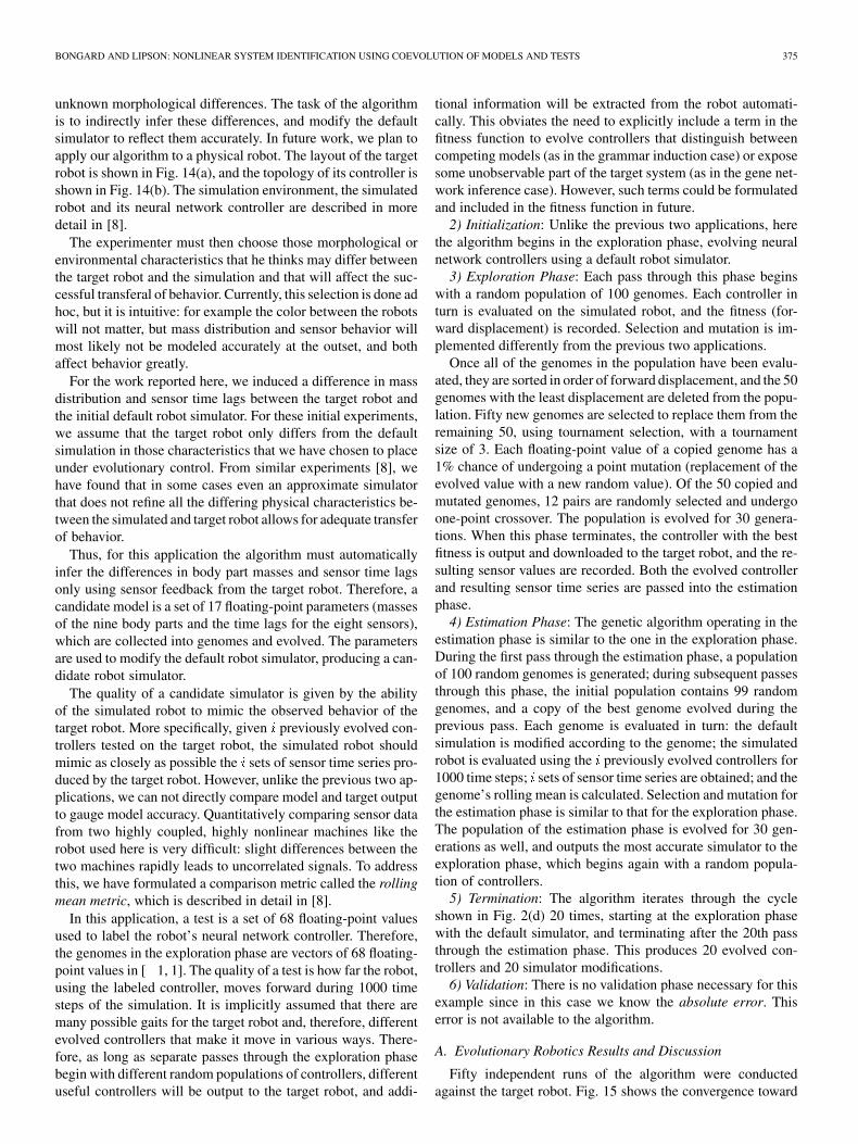
unknown morphological differences. The task of the algorithmis to indirectly infer these differences, and modify the defaultsimulator to reflect them accurately. In future work, we plan toapply our algorithm to a physical robot. The layout of the targetrobot is shown in Fig. 14(a), and the topology of its controller isshown in Fig. 14(b). The simulation environment, the simulatedrobot and its neural network controller are described in moredetail in [8].

The experimenter must then choose those morphological orenvironmental characteristics that he thinks may differ betweenthe target robot and the simulation and that will affect the suc-cessful transferal of behavior. Currently, this selection is done adhoc, but it is intuitive: for example the color between the robotswill not matter, but mass distribution and sensor behavior willmost likely not be modeled accurately at the outset, and bothaffect behavior greatly.

For the work reported here, we induced a difference in massdistribution and sensor time lags between the target robot andthe initial default robot simulator. For these initial experiments,we assume that the target robot only differs from the defaultsimulation in those characteristics that we have chosen to placeunder evolutionary control. From similar experiments [8], wehave found that in some cases even an approximate simulatorthat does not refine all the differing physical characteristics be-tween the simulated and target robot allows for adequate transferof behavior.

Thus, for this application the algorithm must automaticallyinfer the differences in body part masses and sensor time lagsonly using sensor feedback from the target robot. Therefore, acandidate model is a set of 17 floating-point parameters (massesof the nine body parts and the time lags for the eight sensors),which are collected into genomes and evolved. The parametersare used to modify the default robot simulator, producing a can-didate robot simulator.

The quality of a candidate simulator is given by the abilityof the simulated robot to mimic the observed behavior of thetarget robot. More specifically, given previously evolved con-trollers tested on the target robot, the simulated robot shouldmimic as closely as possible the sets of sensor time series pro-duced by the target robot. However, unlike the previous two ap-plications, we can not directly compare model and target outputto gauge model accuracy. Quantitatively comparing sensor datafrom two highly coupled, highly nonlinear machines like therobot used here is very difficult: slight differences between thetwo machines rapidly leads to uncorrelated signals. To addressthis, we have formulated a comparison metric called the rollingmean metric, which is described in detail in [8].

In this application, a test is a set of 68 floating-point valuesused to label the robot’s neural network controller. Therefore,the genomes in the exploration phase are vectors of 68 floating-point values in [ 1, 1]. The quality of a test is how far the robot,using the labeled controller, moves forward during 1000 timesteps of the simulation. It is implicitly assumed that there aremany possible gaits for the target robot and, therefore, differentevolved controllers that make it move in various ways. There-fore, as long as separate passes through the exploration phasebegin with different random populations of controllers, differentuseful controllers will be output to the target robot, and addi-

tional information will be extracted from the robot automati-cally. This obviates the need to explicitly include a term in thefitness function to evolve controllers that distinguish betweencompeting models (as in the grammar induction case) or exposesome unobservable part of the target system (as in the gene net-work inference case). However, such terms could be formulatedand included in the fitness function in future.

2) Initialization: Unlike the previous two applications, herethe algorithm begins in the exploration phase, evolving neuralnetwork controllers using a default robot simulator.

3) Exploration Phase: Each pass through this phase beginswith a random population of 100 genomes. Each controller inturn is evaluated on the simulated robot, and the fitness (for-ward displacement) is recorded. Selection and mutation is im-plemented differently from the previous two applications.

Once all of the genomes in the population have been evalu-ated, they are sorted in order of forward displacement, and the 50genomes with the least displacement are deleted from the popu-lation. Fifty new genomes are selected to replace them from theremaining 50, using tournament selection, with a tournamentsize of 3. Each floating-point value of a copied genome has a1% chance of undergoing a point mutation (replacement of theevolved value with a new random value). Of the 50 copied andmutated genomes, 12 pairs are randomly selected and undergoone-point crossover. The population is evolved for 30 genera-tions. When this phase terminates, the controller with the bestfitness is output and downloaded to the target robot, and the re-sulting sensor values are recorded. Both the evolved controllerand resulting sensor time series are passed into the estimationphase.

4) Estimation Phase: The genetic algorithm operating in theestimation phase is similar to the one in the exploration phase.During the first pass through the estimation phase, a populationof 100 random genomes is generated; during subsequent passesthrough this phase, the initial population contains 99 randomgenomes, and a copy of the best genome evolved during theprevious pass. Each genome is evaluated in turn: the defaultsimulation is modified according to the genome; the simulatedrobot is evaluated using the previously evolved controllers for1000 time steps; sets of sensor time series are obtained; and thegenome’s rolling mean is calculated. Selection and mutation forthe estimation phase is similar to that for the exploration phase.The population of the estimation phase is evolved for 30 gen-erations as well, and outputs the most accurate simulator to theexploration phase, which begins again with a random popula-tion of controllers.

5) Termination: The algorithm iterates through the cycleshown in Fig. 2(d) 20 times, starting at the exploration phasewith the default simulator, and terminating after the 20th passthrough the estimation phase. This produces 20 evolved con-trollers and 20 simulator modifications.

6) Validation: There is no validation phase necessary for thisexample since in this case we know the absolute error. Thiserror is not available to the algorithm.

A. Evolutionary Robotics Results and Discussion

Fifty independent runs of the algorithm were conductedagainst the target robot. Fig. 15 shows the convergence toward


Fig. 15. Convergence toward the physical characteristics of the target robot. Each pass through the estimation phase produces a set of mass changes for each ofthe nine body parts of the robot (top row) and a set of time lags for each of the eight sensors of the robot (bottom row). The trajectories indicate the mean andstandard deviation of the best guesses output by the estimation phase from the 50 independent runs. The each bar corresponds to the best guesses from that passthrough the estimation phase. The open circles indicate the actual differences between the target robot and the starting default simulated robot (for example, thefirst body part of the target robot is 1.5 kg heavier than the corresponding body part of the default simulated robot).

Fig. 16. Behavior recovery after controller transferal. After the first pass through the exploration phase, the best evolved controller caused the simulated robotto move as shown in (a) the trajectory of its center of mass is given by the thin line. The same controller was then supplied to the target robot, and the resultingtrajectory of its motion is given by the thick line. The movement of the updated simulated robot after the 20th pass through the exploration phase (using the newbest evolved controller) is given by the thin line in (b). The motion of the target robot using the same controller is given by the thick line in (b). The horizontal axisindicates forward distance, and the vertical axis indicates height (both are in meters).

the actual mass distribution and sensor time lags of the targetrobot. The figure makes clear that for all 50 runs, the algorithmwas better able to infer the time lags of the eight sensors thanthe mass increases of the nine body parts (indicated by the con-vergence of the means and the negligible standard deviationstoward the actual time lags on the bottom row compared withthe large standard deviations on the top row). In the inferenceof the time lags, the algorithm only had difficulty with sensor3, and tended to overestimate its particular lag. Also, the algo-rithm tended to have difficulty converging on the correct massincreases of most of the body parts, but did a relatively goodjob inferring the mass changes of body parts 4 and 8.

The fact that the algorithm had more difficulty with someparts of the robot and not others is not surprising: the asym-metric mass distribution of the robot causes some aspects of therobot’s morphology to be more observable than others. For ex-ample, the time lag of a touch sensor, attached to a very heavyleg that is only ever dragged along the ground plane (such thatthe sensor always fires), is much more difficult to infer than an-other touch sensor attached to a leg that repeatedly touches theground and lifts off again. Also, a sensor with a shorter time lagis probably easier to infer than one that has a long time lag.

Another reason that it was easier for the algorithm to infersensor rather than body part characteristics is that the sensorsthemselves provide feedback about the robot. In other words,the algorithm automatically, and after only a few target trials,deduces the correct time lags of the target robot’s sensors, butis less successful at indirectly inferring the masses of the bodyparts using the sensor data. As discussed in the previous twosections, often some of the components in a target system (in

this case, an asymmetric robot) are less observable than othercomponents.

One of the runs was selected at random, and the gait of thesimulated robot was compared against the gait of the targetrobot, when both used the same evolved controller. Fig. 16(a) in-dicates the change in behaviors when the first evolved controllerwas transferred, and Fig. 16(b) shows the behavior change whenthe 20th evolved controller was transferred, during the last iter-ation through the algorithm’s cycle.

This figure shows that even with an approximate descriptionof the robot’s mass distribution, the simulator is improvedenough to allow smooth transfer of controllers from simulationto the target robot. Using the default, approximate simula-tion, there is a complete failure of transferal, as indicatedby Fig. 16(a): the target robot simply moves randomly, andachieves no appreciable forward locomotion.

After 20 iterations through the algorithm, an improved sim-ulator is available to the exploration phase, which evolves acontroller that allows the simulated robot to move forward, al-though not as far as the original simulated robot [indicated bythe shorter trajectory in Fig. 16(b) compared with Fig. 16(a)].This is most likely due to the fact that the simulator is now ac-curately modeling the heavier mass of the target robot. Also, thenew gait causes the robot to hop [indicated by the large verticalcurves of the robot’s center of mass in Fig. 16(b)] instead ofwalk [indicated by the steady trajectory of Fig. 16(a)]. In con-trast to the first pass, the target robot exhibits very similar be-havior to the simulated robot when it uses the same controller:both travel a similar distance (about 6.5 m), and both move in


Fig. 17. Average transferal success after each target trial. The light gray barsindicate the average distance traveled by the simulated robot using the bestevolved controller output by that pass through the exploration phase, over all50 runs. The dark gray bars indicate the average distance traveled by the targetrobot using the same controller, during each target trial. Error bars indicate twounits of standard deviation.

the same way (both exhibit a hopping gait that produces trajec-tories with similar frequencies and amplitudes).

Finally, for each pass through the exploration phase, the dis-tance traveled by the simulated robot using the best evolved con-troller was averaged over all the 50 runs. Similarly, the distancetraveled by the target robot using the same controller was aver-aged over the 50 runs. The results are shown in Fig. 17, whichindicates that improvement in behavior transferal success, evenusing an approximate simulator, is a general phenomenon. Onaverage, over the 50 independent runs, there is a drop by 50%in the distance traveled by the target robot, compared with thedefault simulated robot. After about five iterations through thealgorithm’s cycle there is only a statistically insignificant de-crease in distance traveled between the two robots. Althoughnot shown in Fig. 17, this similar distance is matched in all ofthe cases viewed by a qualitative similarity in gait patterns, asshown for a single run in Fig. 16(b).

In this section, we have shown that the estimation-explorationalgorithm can be used to automatically evolve an accurate robotsimulator. Even if the simulator does not describe the targetrobot perfectly, it does allow for automated transferal of evolvedcontrollers from simulation to the target robot. Moreover, suc-cessful transferal becomes possible after only three or four targettrials. In the next section, we extend this approach to automatethe process of diagnosis and recovery for robots that undergosome unanticipated malfunction.

VI. APPLICATION 4: DAMAGED ROBOT RECOVERY

For a robot to function for long periods of time in a hos-tile, unknown or remote environment, it must be able to dealautonomously with uncertainty: specifically, unanticipated in-ternal damage or external environmental change. The recent dif-ficulties with Jet Propulsion Laboratory’s two Mars rovers pro-vide a dramatic example: both robots suffered different, unantic-ipated partial failures [42]. Automatic recovery is most acute insuch instances where human operators cannot manually repairor provide compensation for failure. In this work, we are con-cerned with catastrophic, highly nonlinear robot faults that re-quire recovery controllers qualitatively different from the orig-inal controller.

Some work has been done on employing evolutionary algo-rithms to restore functionality after some unanticipated damagehas occurred, but all of this work relies on massive numbers ofhardware trials: robot recovery has been demonstrated in [4] and[47], and for electronic circuits in [10] and [37]. However, re-peated generate-and-test algorithms for robotics is not desirablefor several reasons: repeated trials may exacerbate damage anddrain limited energy; long periods of time are required for re-peated hardware trials; damage may require rapid compensation(e.g., power drain due to coverage of solar panels); and repeatedtrials continuously change the state of the robot, making damagediagnosis difficult.

Grefenstette and Ramsey [28] propose an algorithm for con-tinual behavioral learning in a robot context which does not re-quire large numbers of target trials. However, their system as-sumes that changes in the robot’s environment (in their case,speed change of a prey robot) can be directly inferred usingsensor data and provided to the behavior learning component. Intheir case, it is assumed that the prey robot may change speed,and their described algorithm assumes that speed change can bedetected by the predator robot; the observed change in then feddirectly into the predator’s behavior learning component. How-ever, the more difficult aspect of damage diagnosis and recoveryis usually diagnosis: in the estimation-exploration algorithm itis assumed that robot or environmental changes are not knownin advance, and must be inferred indirectly using the sensorsthat also drive behavior. Grefenstette and Ramsey state that in-direct sensing of environmental change could be included intotheir system, but they do not provide any description as to howthis could be accomplished.

As mentioned in the previous section, several types of plasticneural network controllers have been proposed that allow forrapid, lifetime adaptation to external perturbation (e.g., [19],[24] and [60]). Furthermore, Keymeulen et al. [36] have formu-lated an algorithm that continuously updates an internal modelof sensor input/world response data obtained from a wheeledrobot, and uses this model to evolve and download controllersto the robot during task execution. They have demonstrated thattheir algorithm greatly reduces the number of required hardwaretrials, compared with a similar model-free algorithm. However,none of these approaches generate a hypothesis describing whatparticular change the robot or its environment has experienced.Second, the evolved controllers have not been shown capable offundamental reorganization when faced with unanticipated, cat-astrophic failure (such as the separation of a limb), as is demon-strated here for our proposed algorithm.

Srinivas [57] was one of the first researchers to study error di-agnosis and recovery, but his approach, along with subsequentapproaches ([1], [11], [20], [35], [61]), require online operation(repeated testing on the physical robot), and cannot handle unan-ticipated errors. Baydar and Saitou [4] proposed the first offlineerror diagnostic and recovery system, which relies on Bayesianinference for error diagnosis, and genetic programming [40] forerror recovery. However, their algorithm also only handles pre-specified error types.

Mahdavi and Bentley [47] recently demonstrated an onlineevolutionary algorithm that automatically recovers behavior fora physical robot. However, after damage the physical robot re-quired 400 hardware trials and nearly seven hours to recover


Fig. 18. Parsing of an example genome in the estimation phase. This particular genome has one active and three inactive genes. The resulting single modification(a weakening of the third motor by 43%) is applied to the default simulator.

72% of its original functionality. Their approach is similar tothat portrayed in Fig. 13: evolution is continued on the targetrobot after transferal.

Here, we describe the application of the estimation-explo-ration algorithm to the problem of damaged robot recovery,which, for the results presented here, requires only ten targettrials (on average) to restore functionality. Like the previousapplication, the algorithm automatically evolves two separatestructures: a robot simulator that explains unanticipated internaldamage or external environmental change suffered by the targetrobot; and a compensatory neural network controller that re-stores functionality to the target robot, given the evolved robotsimulator. Below, we outline the application of the first fivesteps of the proposed algorithm to the problem of automateddamage diagnosis and recovery; validation, as in the previousapplications, is not used here.

1) Characterization of the Target System: Like the previousapplication, the target robot is an independent simulated robotthat possesses some unknown differences in contrast to aninitial, approximate simulator. We use the same quadrupedalrobot as before (Fig. 14), but the target robot no longer has alarger mass and time-delayed sensors, but does suffer some un-expected malfunction or environmental change. The algorithmmust then diagnose this malfunction using sensory feedback asbefore, and update the simulator to reflect this damage: if thetarget robot has lost a leg, then a good simulator must simulatea robot with the correct leg missing.

The model in this application is a genome that can encodezero to four simultaneous malfunctions. Each encoded malfunc-tion is parameterized as to: which body part, joint, sensor, ormotor it applies; what has happened (the joint has broken orthe sensor has failed); and how severe the damage is (expressedas a percentage). Genomes are comprised of 16 floating-pointvalues, and each genome is divided into four genes, each com-prised of four values; each gene describes a possible malfunc-tion. These values are parsed into a set of malfunctions to applyto the default simulated robot. Fig. 18 outlines a sample genomebeing parsed; refer to [8] for more details regarding the specificsof the genetic encoding. Thus, each genome produces some

modification of the simulated robot and its environment; thissimulation is treated as the candidate model. The quality of amodel is again the ability of the given simulated robot to mimicthe behavior of the crippled target robot.

This encoding gives a search space of 20010 different genomes. As the values are discretized,there are at most

possible sets of simulator modifications, although some ofthese are not unique because ordering is irrelevant, multiplemodifications can be additive (two weakenings of the samemotor by 10% is equivalent to one weakening of the samemotor by 20%) and modifications encoded by inactive genesare not applied.

A test in this application is the same as for the previous ap-plication: genomes encode a vector of 68 synaptic weights forthe controller. The quality of a labeled controller is how far itenables the crippled robot to move forward during 1000 timesteps of the simulation.

2) Initialization: As in the previous application, we begin witha default simulation of the quadrupedal robot and its environ-ment, and initiate the exploration phase to evolve a neural net-work controller for it. The best evolved controller is then down-loaded onto the damaged target robot, and the resulting sensorydata, along with the evolved controller, are fed into the estima-tion phase in order to improve the simulation.

3) Exploration Phase: During each pass through the explo-ration phase a population of 200 genomes is evolved for 40generations. Before each evaluation, the default simulator ismodified (i.e., the simulated robot is damaged) according to theevolved set of modifications supplied by the estimation phase.Selection and mutation are implemented the same way as in theprevious application. At the end of this phase, the best controlleris output to the target robot.

4) Estimation Phase: Each pass through the estimation phasebegins with a random population of 200 genomes; on the secondand subsequent passes through this pass, the random populationis seeded with the best simulator modification evolved duringthe previous pass. Each genome in turn is parsed; the resulting


TABLE IIUNANTICIPATED SITUATIONS TESTED

modifications (if any) are applied to the default simulator; themodified simulated robot is evaluated using the controllers al-ready tested on the target robot; and both the sensor logs fromthe damaged target robot and those obtained from the simula-tion are compared using the rolling mean metric [8] to assessthe accuracy of the current genome. Once all of the genomes inthe population have been evaluated, the population is sorted ac-cording to accuracy, and selection, mutation and crossover is ap-plied. Each pass through the estimation phase evolves the pop-ulation for 40 generations. At the end of the pass, the best set ofsimulator modifications is passed to the exploration phase.

5) Termination: Starting at the exploration phase, the algo-rithm iterates through the cycle shown in Fig. 2(e) ten times,leading to ten evolved controllers, ten target tests, and tenevolved simulations. See Table I for a summary of the applica-tion of the estimation-exploration algorithm to this problem.

6) Validation: There is no validation phase necessary for thisexample since in this case we know the absolute error. Thiserror is not available to the algorithm.

A. Damaged Robot Recovery Results and Discussion

Thirteen different target robots were tested: each suffered adifferent unanticipated situation. Table II describes the situa-tions. The algorithm was then run 20 times against each of the13 target robots. The estimation phase attempts to evolve simu-lator modifications that will describe this situation: for each ofthe 13 situations, there are only a few genomes (or none, in thecase of situations 11–13) that will describe it perfectly, out ofthe 86 400 possible situations. Each run requires about 4 h ofcomputation on a 1 GHz PC.

Fig. 19 documents the performance of a single run of thecontrol algorithm against a target robot that has suffered a 50%failure of one of its touch sensors (situation 5 in Table II). Thealgorithm evolves an approximate description of the damageafter the first target test, and evolves a perfect description afterthe second test. This indicates that as the algorithm accumulatesmore data from the target robot by causing it to behave in dif-ferent ways, it is better able to model the target robot’s situation.Also, Fig. 19(a) shows that, armed with an accurate model after

Fig. 19. (a) The evolutionary progress of a sample run against situation 5:one of the angle sensors breaks by 50%. The dotted lines indicate the progressof the first five passes through exploration phase. The captions indicate the bestsimulator modifications evolved by four passes through the estimation phase.The triangle shows the original distance traveled by the target robot. The circleindicates distance traveled after suffering the failure. The squares indicatethe distance traveled by the damaged target robot during each of the fourtrials. (b)–(d) Images of the target robot’s motion: (b) before the unanticipatedsituation; (c) after encountering the unanticipated situation; and (d) during thefifth target trial.

Fig. 20. Automated recovery after a catastrophic failure using the proposedalgorithm. (a) The behavior of the default simulated robot using the bestcontroller evolved during the first pass through the exploration phase. (b) Thetarget robot has lost part of a leg through joint separation, and the robot attemptsto move using the first evolved controller. (c) The motion of the damaged targetrobot during the second target trial.

the second test, the algorithm is able to evolve a compensatorycontroller for the damaged robot that restores functionality.

Fig. 20 indicates that the proposed algorithm is even able toprovide compensatory controllers when the target robot sufferscatastrophic failure, such as a change in the robot’s topology(one of the lower legs has broken off, represented by situation3 from Table II). Here, the algorithm correctly identifies the


Fig. 21. The average performance of the proposed algorithm against all 13damaged robots. The algorithm was run ten times against each situation. Thewhite bars indicate the average distance traveled by the default simulated robotusing the first evolved controller. The light gray bars indicate the averagedistance traveled by the target robot during the first target trial. The dark graybars indicate the average distance traveled by the target robot during the tenthtarget trial.

damage after the second pass through the estimation phase, andthe exploration phase uses this accurate simulator to evolve anew controller that allows the damaged robot to move using onlythree legs. Note the difference in trajectories shown in Fig. 20(a)and (c): the original gait caused the robot to move using longhops [indicated by the long loops in Fig. 20(a)], but the damagedrobot uses a compensatory controller that causes it to move inshort, hesitant hops] indicated by the short loops in Fig. 20(b)].Thus, the algorithm automatically diagnoses mild or severe mal-function, and either modifies the gait slightly over subsequenttrials or evolves a qualitatively different gait, depending on thedamage incurred.

Fig. 21 reports the ability of the proposed algorithm to recoverfunction for damaged robots. The algorithm was able to restorefunctionality (regarded as a statistically significant increase inmean performance between the first and tenth hardware trial) forall but damage scenarios 6, 11, and 13. Even in these three cases,many of the runs produce a significant increase in performance.Note that even in the catastrophic cases such as 3, 4, 7, and 10(indicated by almost complete lack of forward motion during thefirst hardware trial) some functionality was restored, indicatingthat our algorithm may be useful for recovering some functionfrom severely damaged robots.

Note also that both algorithms were able to successfully re-cover when faced with an unanticipated environmental change:the horizontal canting of the ground plane (situation 10). Thiswas probably due to the drastic effect on all sensors induced bythis change. It is important to note that the proposed algorithmcan distinguish between internal damage and external environ-mental change, and reconstruct the change in simulation, basedsolely on indirect sensory information.

Most encouragingly, some functionality was restored in cases11 and 12, in which there was no genome that could perfectlydescribe the malfunction. Further study is required in order tounderstand how truly unanticipated situations can best be ap-proximated by a set of simulator modifications.

VII. DISCUSSION

The previous four sections have described the application ofthe estimation-exploration algorithm to four separate problems:grammar induction, gene network inference, the evolution of an

accurate robot simulator, and automated diagnosis and recoveryfrom unanticipated robot malfunction. These four applicationshave not only demonstrated that our approach is problem do-main independent, but have also highlighted its various proper-ties and benefits. Before we summarize the results from theseapplications, however, it is worthwhile to go into more detailabout the differences between the proposed algorithm and othercoevolutionary algorithms.

A. Differences From Pure Coevolutionary Algorithms

The main difference between the estimation-exploration al-gorithm and other coevolutionary systems proposed so far is thatour algorithm is a hybrid system: the fitness of both the modeland test populations is influenced by the opposing population,but also by the behavior of an additional, third component—thetarget system. In other coevolutionary algorithms, the fitness ofan individual is influenced by one or more individuals from an-other (or the same) population. For this reason, the fitness ofa coevolving individual in such systems is purely subjective; itis calculated based only on other individuals. However, in oursystem, there is a static component to search, which is the abilityof a model to mimic the observed behavior of a target system:as long as the target system does not alter its internal structureover time, there is an objective aspect to the search for bettermodels. For this reason, we view previous coevolutionary sys-tems as pure coevolutionary systems, and the estimation-explo-ration algorithm as a hybrid coevolutionary system.

B. Application of the Algorithm

In the grammar induction problem, it was shown that an in-telligent test is often one that distinguishes between alterna-tive candidate models, a concept related to that propounded inthe competitive coevolutionary literature: the quality of an indi-vidual in one population is proportional to its ability to induce aperformance gradient in the subset of individuals challenging itfrom the competing population [12], [22], [33]. There are sev-eral reasons cited as to why such a test is desirable, but there isa specific advantage in the context of the estimation-explorationalgorithm, described next.

If a test does not induce disagreement between models, andthe test is passed to the target DFA for classification, then onthe subsequent pass through the estimation phase there will bean absolute but not a relative change in the fitnesses of the bestmodels: the fitnesses of the best models from each subpopu-lation will either all go up by one (if they match the classifica-tion of the target DFA) or down by one (if they disagree withthe target DFA). If the best models all improve in fitness, thereis little chance for evolutionary improvement: new models canonly classify any previous sentences not yet correctly classifiedby the current best models, if there are any. If the best models allexperience a drop in fitness, then there is sufficient room for im-provement: a new model may correctly classify all the sentencesthat the best model(s) do, as well as the new sentence that theydo not.

However, as the inference process proceeds, and the modelsin the estimation phase improve, there is an increasing likeli-hood that the best models will correctly classify any incomingsentence. Therefore, there will be a diminishing return over the


inference process of proposing sentences for classification thatthe best models already agree on. However, if a sentence is pro-posed for classification by the target DFA that causes disagree-ment among the best models, there is a guarantee that of thebest models will incorrectly classify the new sentence, therebyensuring the possibility of further model improvement.

Tests that cause model disagreement have an added benefit:it helps to uncover less observable components of the targetsystem. For example, in the grammar induction application, in-telligent testing tended to elicit much more balanced classifi-cations from unbalanced target DFAs than random testing wasable to [see Fig. 7(c)]. For many of these unbalanced DFAs, theproposed algorithm was able to extract enough of the minorityclassifications using intelligent testing to evolve a much moreaccurate model, on average, than the same algorithm but withrandom testing. In such cases when the hidden system has lowobservability, tests must be formulated that produce more of theunderrepresented output in order to infer the internal structureof the system: in the estimation-exploration algorithm this oc-curs as a natural result of evolving tests that cause disagreementamong models.

For the gene network inference problem, we have shown thatit is possible to automatically evolve the regulatory connec-tions between a set of genes given a set of input and outputgene product concentrations. Moreover, our approach does notrequire invasive, expensive, slow, and disruptive experimentssuch as knockout or lesion studies. Rather, the exploration phasecarefully evolves a low-cost experiment (a set of initial chemicalconcentrations that trigger gene regulation) that yields a largeamount of information about the physical system.

Like the grammar induction problem, it was found thatevolving useful tests, instead of proposing random ones, speedsthe discovery of accurate gene network models, thus requiringa minimum of physical experimentation. Moreover, it wasfound that the usefulness of evolving tests increases as problemdifficulty increases: it was found that evolving tests is increas-ingly useful as the hidden gene networks increase in size andconnectivity. This finding bodes well for the scalability of ourapproach, suggesting that our algorithm may prove very usefulfor genetic network inference in particular, and for systemsbiology research in general.

In Section V, we described the application of the estima-tion-exploration algorithm to the problem of automaticallygenerating controllers for robots. In that application the hiddentarget system is a robot with unknown morphological differ-ences compared with an initial default simulated robot. Thealgorithm evolves controllers for the robot in simulation, whichare then tested on the target robot. The resulting sensor data,along with the evolved controller, serve as input/output datapairs which are used to evolve improvements to the robot sim-ulator. It was shown that this approach automatically producesaccurate enough simulators for the successful transferal of con-trollers from simulation to the target robot, using a minimum oftrials on the target robot. This approach is appealing because:repeated testing on a physical robot is time-consuming andpotentially damaging; the sensors already being used to drivebehavior also act as diagnostic sensors, returning indirect infor-mation about the target robot’s morphological characteristics;

and our approach could be combined with other approachesthat have already been suggested for automating the process ofevolved controller transferal.

In the last application, we employed the estimation-explo-ration algorithm to automatically diagnose unanticipated mal-functions suffered by the target robot, and automatically evolvecompensatory controllers for it. As in the previous three appli-cations, recovery was achieved with a small number of targettrials. In this application a maximum of ten target trials were suf-ficient to restore functionality in the face of: minor, catastrophic,or compound damages; no damage at all; changes in the robot’senvironment; or malfunctions that could not be perfectly ex-pressed in simulation. Most importantly, the algorithm was ableto automatically distinguish and describe these diverse situa-tions using only sensory feedback and the rolling mean metric,which quantitatively compares behaviors between highly cou-pled, highly nonlinear dynamic robots. Once a correct diag-nosis is discovered the algorithm is often able to evolve a com-pensatory controller, often evolving qualitatively different gaitsin response to fundamental changes experienced by the targetrobot.

C. Model Accuracy Versus Structural Accuracy

When performing system identification, it is possible to gen-erate a model that successfully mimics the input–output be-havior of the target system, which we refer to as model accu-racy, but fails to reflect the actual internal structure of the targetsystem, which we call structural accuracy. Whether our pro-posed algorithm actually captures structural as well as modelaccuracy depends on the specific application.

For grammar induction, there are often several DFAs that pro-duce identical classifications. So for this application, it is impos-sible to determine, using any algorithm, whether a model DFAhas captured the actual internal structure of the target DFA: ab-solute error of a candidate model is simply approximated usinga large set of previously unseen sentences.

In the gene network application, our algorithm does capturethe internal structure of the target gene networks: absolute erroris considered to be the distance between the internal structuresof the model and target networks. As can be seen in Fig. 9(d),the internal structures of the best model gene networks producedby the estimation-exploration algorithm are closer to those ofthe target networks than those models produced by the othertwo algorithms (indicated by the final absolute errors of the bestmodels). However, this correlation between model and struc-tural accuracy depends on the way in which we have chosento model gene networks: validation methods for determiningwhether a given gene network model actually captures the regu-lation inherent in an actual biological gene network is currentlybeing investigated.

In the case of the first robot application, Fig. 15 indicates thatall of the runs tend to converge on the actual internal structureof the target system: the mass distribution and sensor time lagsof the target robot. In the case of the second robot application,Table II reports that for many of the damage scenarios, the esti-mation-exploration algorithm actually discovers the perfect de-scription of the damage (see column 3). However, for these twoapplications we are most interested in determining how well the


TABLE IIIALGORITHM INFERENCE ABILITY

algorithm can approximate an indescribable structural changeto the robot or its environment and recover from it.

D. Comparison of Performance

Table III summarizes the inference ability of the algorithmfor the grammar induction and gene network inference applica-tions. The first row reports that for 21 of the 30 target DFAs,the estimation-exploration algorithm was able to find a perfectmodel using fewer target evaluations than the other two controlalgorithms [see Fig. 7(b)]. The remaining nine targets showedno statistical improvement using intelligent testing. Moreover,for 14 of the 30 target DFAs, the proposed algorithm discovereda perfect model using significantly fewer model evaluations [seeFig. 7(a)]. In the case of gene network inference, all three algo-rithms performed 10 model evaluations, the standard GAperformed 100 target evaluations, the iterative algorithm withrandom testing performed 56 target evaluations and the estima-tion-exploration algorithm performed 55 target evaluations. Ascan be seen from Table III, the proposed algorithm consistentlyproduces more accurate models for large and more densely con-nected gene networks (see Fig. 9). This indicates that the esti-mation-exploration algorithm is scalable: intelligent testing be-comes increasingly useful as the size of the target system in-creases and its observability decreases.

Table IV summarizes the recovery ability of the proposed al-gorithm for the latter two robot applications. In the third appli-cation, the target robot had a different mass distribution and sig-nificant sensor time lags, compared with its corresponding robotsimulator. As a control, a neural controller was evolved directlyon this target robot using the genetic algorithm described in Sec-tion V. Ten independent runs of this control were performed.After 600 evaluations in each run, the best controller was ex-tracted, and the mean distance achieved by the robot using theseten networks in turn was found to be 5.3 m. The intervals inthis table represent standard deviation, indicating the distribu-tion of distances traveled by the best robot from each run, forboth algorithms. Both the means and the standard deviations

TABLE IVALGORITHM RECOVERY ABILITY

indicate that in this case, the estimation-exploration algorithmcaused the target robot to achieve the same performance as thecontrol algorithm, in which all evolution is performed directlyon the target robot, but using only 20 physical tests, comparedwith 600. Thus, there was an order of magnitude improvementin extracting a desired behavior from the target robot.

A similar control was devised for the damaged robot recoveryapplication. Again a genetic algorithm was used to evolve neuralcontrollers directly on the target robot, which in this case wasa damaged quadrupedal robot (one of the lower legs separatescompletely from the body). In this case, even after 1550 evalu-ations (evolving a population of 100 controllers for 30 genera-tions), only half of the mean distance was achieved comparedwith the mean distance traveled by the target robot after tenphysical tests using the proposed algorithm. Although there isa slight overlap in the standard deviations, it is clear that theproposed algorithm performs better than simply evolving con-trollers directly on the target robot, using two orders of magni-tude fewer target trials (1500 versus 10).

VIII. CONCLUSION

We have introduced the estimation-exploration algorithm,a coevolutionary approach to system identification. We haveshown how our algorithm differs from other pure coevolu-tionary systems because it does not so much introduce a newadvance in coevolutionary theory, but rather introduces a sys-tematic, domain independent method for performing synthesisor analysis using coevolution.

Unlike other coevolutionary systems, the estimation-explo-ration algorithm evolves candidate models that are influencednot only by the competing population of tests, but also by thetarget system. This removes two potential pathologies from thealgorithm (cycling and overspecialization) which are often suf-fered by other coevolutionary algorithms. The third pathology,disengagement, has been observed to occur in our algorithm, butnot for the four applications shown here. We have formulatedtwo mechanisms that combat disengagement, and are currentlyinvestigating additional mechanisms.

We have documented its application to four very differentproblems, thus demonstrating its problem domain indepen-dence. The algorithm has several other benefits that have beenhighlighted in the various applications: coupled automation ofboth models and intelligent tests; the active minimization oftarget testing; increased usefulness as target systems increasein size and complexity; increased usefulness for target systems


with low observability; and automating the extraction of usefulbehavior from a hidden system.

Thus, our algorithm performs well at inference: it can au-tomatically construct a hidden system that explains the gath-ered data. Active learning is also concerned with the intelli-gent selection of tests [16], but in that domain a classifier isused to describe input/output relations; no explicit model of thetarget system is generated. This is an important distinction tomake, because by building explicit models to explain the datarather than learning an approximation of the input/output rela-tionships, we obtain several benefits:

1) we can use the resultant model to learn more about thehidden system (we can use it to test hypotheses about theactual system);

2) we can uncover possible causalities rather than just cor-relations (“gene regulates gene ,” rather than “the ex-pressions of genes and are correlated”);

3) we can obtain a comprehensible description of somechange in the hidden system (such as what damage hasincurred, and where);

4) we can generate some useful behavior for it (continuationof function by circumventing the damage).

The third and fourth property allow us to recover functionfrom the hidden system using a minimum number of tests.Second, unlike active learning, tests can be constructed, al-lowing for the exploration of a possibly infinite space of tests,rather than selected from some fixed space of tests with equaldimensionality.

Furthermore, using evolution allows us to synthesize modelsand tests for systems about which little is known. This is impor-tant in nonlinear black-box system identification tasks for whichnot even the underlying topology of the hidden system is known[56]. Artificial evolution could be used to build explicit modelsdirectly from observed data in such instances, a challenge thathas not yet been addressed in the system identification literature,to the best of the authors’ knowledge. For example the algorithmcould be used in a remote robotics application to synthesize amodel of a novel environment based only on the robot’s sensordata: this is an attractive avenue for future study. In future work,we also plan to apply the algorithm to a range of actual physicalsystems, including physical robots and real biological networks.

REFERENCES

[1] M. G. Abu-Hamdan and A. S. El-Gizawy, “Computer aided monitoringsystem for flexible assembly operations,” Comput. Ind., vol. 34, pp.1–10, 1997.

[2] A. Adamatzky, M. Komosinski, and S. Ulatowski, “Software review:Framsticks,” Kybernetes: Int. J. Syst. Cybern., vol. 29, pp. 1344–1351,2000.

[3] A. Arkin, P. Shen, and J. Ross, “A test case for correlation metric con-struction of a reaction pathway from measurements,” Science, vol. 277,pp. 1275–1279, 1997.

[4] C. M. Baydar and K. Saitou, “Off-line error prediction, diagnosis andrecovery using virtual assembly systems,” in Proc. IEEE Int. Conf.Robotics Autom., 2001, pp. 818–823.

[5] F. Bergadano and D. Gunetti, Inductive Logic Programming: From Ma-chine Learning to Software Engineering. Cambridge, MA: MIT Press,1995.

[6] J. Bongard and H. Lipson, “‘Managed challenge’ alleviates disengage-ment in coevolutionary system identification,” in Proc. Genetic Evol.Comput. Conf., 2005, pp. 531–538.

[7] J. Bongard and R. Pfeifer, “Repeated structure and dissociation of geno-typic and phenotypic complexity in artificial ontogeny,” in Proc. GeneticEvol. Comput. Conf., 2001, pp. 829–836.

[8] J. C. Bongard and H. Lipson, “Automated robot function recovery afterunanticipated failure or environmental change using a minimum of hard-ware trials,” in Proc. NASA/DoD Conf. Evolvable Hardware, Seattle,WA, 2004, pp. 169–176.

[9] J. C. Bongard and H. Lipson, “Automating genetic network inferencewith minimal physical experimentation using coevolution,” in Proc. Ge-netic Evol. Comput. Conf., Seattle, WA, 2004, pp. 333–345.

[10] D. W. Bradley and A. M. Tyrrell, “Immunotronics: Novel finite-state-machine architectures with built-in self-test using self-nonself differen-tiation,” IEEE Trans. Evol. Comput., vol. 6, no. 3, pp. 227–238, Jun.2002.

[11] S. Brnyjolfsson and A. Arnstrom, “Error detection and recovery in flex-ible assembly systems,” Int. J Adv Manuf. Technol., vol. 5, pp. 112–125,1990.

[12] A. Bucci, J. B. Pollack, and E. D. De Jong, “Automated extraction ofproblem structure,” in Proc. Genetic Evol. Comput. Conf., 2004, pp.501–512.

[13] T. Chen, H. L. He, and G. M. Church, “Modeling gene expression withdifferential equations,” in Proc. Pacific Symp. Biocomput., vol. 4, 1999,pp. 29–40.

[14] O. Cicchello and S. C. Kremer, “Inducing grammars from sparse datasets: A survey of algorithms and results,” J. Mach. Learn. Res., vol. 4,pp. 603–632, 2003.

[15] D. Cliff and G. F. Miller, “Tracking the red queen: Measurements ofadaptive progress in coevolutionary simulations,” in Proc. Eur. Conf.Artif. Life, 1995, pp. 200–218.

[16] D. Cohn, L. Atlas, and R. Ladner, “Improving generalization with activelearning,” Mach. Learn., vol. 15, no. 2, pp. 201–221, 1994.

[17] H. de Jong, “Modeling and simulation of genetic regulatory systems: Aliterature review,” J. Comput. Biol., vol. 9, no. 1, pp. 69–105, 2002.

[18] P. D’haeseleer, S. Liang, and R. Somogyi, “From co-expressionclustering to reverse engineering,” Bioinformatics, vol. 16, no. 8, pp.707–726, 2000.

[19] E. A. DiPaolo, “Homeostatic adaptation to inversion of the visual fieldand other sensorimotor disruptions,” in From Animals to Animats 6, J.A. Meyer, A. Berthoz, D. Floreano, H. L. Roitblat, and S. W. Wilson,Eds. Cambridge, MA: MIT Press, 2000, pp. 440–449.

[20] E. Z. Evans and S. G. Lee, “Automatic generation of error recoveryknowledge through learned activity,” in Proc. IEEE Int. Conf. RoboticsAutom., 1994, pp. 2915–2920.

[21] R. Featherstone and D. E. Orin, “Robot dynamics: Equations and algo-rithms,” in Proc. IEEE Int. Conf. Robotics Autom., 2000, pp. 826–834.

[22] S. G. Ficici and J. B. Pollack, “Pareto optimality in coevolutionarylearning,” in Proc. 6th Eur. Conf. Adv. Artif. Life:, 2001, pp. 316–327.

[23] D. Floreano and F. Mondada, “Evolutionary neurocontrollers for au-tonomous mobile robots,” Neural Netw., vol. 11, pp. 1461–1478, 1998.

[24] D. Floreano and J. Urzelai, “Neural morphogenesis, synaptic plasticity,and evolution,” Theory Biosci., vol. 120, pp. 225–240, 2001.

[25] L. J. Fogel, A. J. Owens, and M. J. Walsh, Artificial Intelligence ThroughSimulated Evolution. New York: Wiley, 1966.

[26] P. Funes and J. Pollack, “Computer evolution of buildable objects,” inEvolutionary Design by Computer, P. Bentley, Ed. San Francisco, CA:Morgan Kauffman, 1999, pp. 387–403.

[27] M. Gevers, “A decade of progress in iterative control design: Fromtheory to practice,” J. Process Control, vol. 12, no. 4, pp. 519–531, May2002.

[28] J. J. Grefenstette and C. L. Ramsey, “An approach to anytime learning,”in Proc. 9th Int. Workshop Mach. Learn., 1992, pp. 189–195.

[29] W. D. Hillis, “Coevolving parasites improve simulated evolution as anoptimization procedure,” Physica D, vol. 42, pp. 228–234, 1990.

[30] G. S. Hornby and J. B. Pollack, “Creating high-level components witha generative representation for body-brain evolution,” Artif. Life, vol. 8,no. 3, pp. 223–246, 2002.

[31] H. Iba and A. Mimura, “Inference of a gene regulatory network by meansof interactive evolutionary computing,” Inf. Sci., vol. 145, pp. 225–236,2002.

[32] N. Jakobi, “Evolutionary robotics and the radical envelope of noise hy-pothesis,” Adaptive Behav., vol. 6, no. 1, pp. 131–174, 1997.

[33] E. D. De Jong and J. B. Pollack, “Ideal evaluation from coevolution,”Evol. Comput., vol. 12, no. 2, pp. 159–192, 2004.

[34] H. Juillé, “Methods for statistical inference: Extending the evolutionarycomputation paradigm,” Ph.D. dissertation, Brandeis Univ., Waltham,MA, May 1999.


[35] J. F. Kao, “Optimal recovery strategies for manufacturing systems,” Eur.J. Oper. Res., vol. 80, pp. 252–263, 1995.

[36] D. Keymeulen, M. Iwata, Y. Kuniyoshi, and T. Higuchi, “Online evolu-tion for a self-adapting robotics navigation system using evolvable hard-ware,” Artif. Life, vol. 4, pp. 359–393, 1998.

[37] D. Keymeulen, A. Stoica, and R. Zebulum, “Fault-tolerant evolvablehardware using field programmable transistor arrays,” IEEE Trans.Reliability (Special Issue on Fault-Tolerant VLSI Syst.), vol. 49, pp.305–316, Sep. 2000.

[38] S. Kikuchi, D. Tominaga, M. Arita, and M. Tomita, “Pathway findingfrom given time-courses using genetic algorithm,” Genome Informatics,vol. 12, pp. 304–305, 2001.

[39] H. Kitano, Foundations of Systems Biology. Cambridge, MA: MITPress, 2001.

[40] J. Koza, Genetic Programming: On the Programming of Computers byMeans of Natural Selection. Cambridge, MA: MIT Press, 1992.

[41] S. Kumar and P. Bentley, On Growth, Form and Computers. New York:Academic, 2003.

[42] NASA Jet Propulsion Laboratory. (2004) Mars exploration rovers. [On-line]. Available: http: //www.jpl.nasa.gov/mer2004/

[43] H. Lipson and J. B. Pollack, “Automatic design and manufacture of ar-tificial lifeforms,” Nature, vol. 406, pp. 974–978, 2000.

[44] L. Ljung, System Identification: Theory for the User. EnglewoodCliffs, NJ: Prentice-Hall, 1999.

[45] S. M. Lucas and T. J. Reynolds, “Learning DFA: Evolution versus evi-dence driven state merging,” in Proc. Congr. Evol. Comput., 2003, pp.351–358.

[46] S. Luke, S. Hamahashi, and H. Kitano, “‘Genetic’ programming,” inProc. Genetic Evol. Comput. Conf., 1999, pp. 1098–1105.

[47] S. H. Mahdavi and P. J. Bentley, “An evolutionary approach to damagerecovery of robot motion with muscles,” in Proc. 7th Eur. Conf. Artif.Life, 2003, pp. 248–255.

[48] E. Mjolsness, D. H. Sharp, and J. Reinitz, “A connectionist model ofdevelopment,” J. Theor. Biol., vol. 152, pp. 429–454, 1991.

[49] B. Olsson, “Coevolutionary search in asymmetric spaces,” Inf. Sci., vol.133, pp. 103–125, 2001.

[50] R. Parekh and V. Honavar, “Automata induction, grammar inference,and language acquisition,” in The Handbook of Natural Language Pro-cessing, R. Dale, H. Moisl, and H. Somers, Eds. New York: MarcelDekker, 2000, pp. 727–764.

[51] J. B. Pollack, H. Lipson, S. Ficici, P. Funes, G. Hornby, and R. Watson,“Evolutionary techniques in physical robotics,” in Evolvable Systems:From Biology to Hardware, J. Miller, Ed. Berlin, Germany: Springer-Verlag, 2000, pp. 175–186.

[52] M. A. Potter and K. A. De Jong, “Cooperative coevolution: An architec-ture for evolving coadapted subcomponents,” Evol. Comput., vol. 8, no.1, pp. 1–29, 2000.

[53] T. Reil and P. Husbands, “Evolution of central pattern generators forbipedal walking in a real-time physics environment,” IEEE Tran. Evol.Comput., vol. 6, no. 2, pp. 159–168, Apr. 2002.

[54] C. D. Rosin and R. K. Belew, “New methods for competitive coevolu-tion,” Evol. Comput., vol. 5, no. 1, pp. 1–29, 1997.

[55] K. Sims, “Evolving 3D morphology and behavior by competition,” Artif.Life IV, pp. 28–39, 1994.

[56] J. Sjöberg, Q. Zhang, L. Ljung, A. Benveniste, B. Delyon, P.-Y. Glo-rennec, H. Hjalmarsson, and A. Juditsky, “Nonlinear black-box mod-eling in system identification: A unified overview,” Automatica, vol. 31,no. 12, pp. 1691–1724, 1995.

[57] S. Srinivas, “Error recovery in robot systems,” Ph.D. dissertation, Calif.Inst. Technol., Pasadena, CA, 1977.

[58] K. O. Stanley and R. Miikkulainen, “Competitive coevolution throughevolutionary complexification,” J. Artif. Intell. Res., vol. 21, pp. 63–100,2004.

[59] A. Thompson, “Artificial evolution in the physical world,” in Evolu-tionary Robotics: From Intelligent Robots to Artificial Life (ER’97), T.Gomi, Ed. Ottawa, ON, Canada: AAI Books, 1997, pp. 101–125.

[60] S. Tokura, A. Ishiguro, H. Kawai, and P. Eggenberger, “The effect ofneuromodulations on the adaptability of evolved neurocontrollers,” inProc. 6th Eur. Conf. Artif. Life, J. Kelemen and P. Sosik, Eds., 2001, pp.292–295.

[61] M. L. Visinsky, J. R. Cavallaro, and I. D. Walker, “Expert system frame-work for fault detection and fault tolerance in robotics,” Comput. Elect.Eng., vol. 20, pp. 421–435, 1994.

[62] R. A. Watson and J. B. Pollack et al., “Coevolutionary dynamics in aminimal substrate,” in Proc. Genetic Evolutionary Comput. Conf., L.Spector and E. D. Goodman, Eds., 2001, pp. 702–709.

[63] V. Zykov, J. Bongard, and H. Lipson, “Coevolutionary variance guidesphysical experimentation in evolutionary system identification,” in Proc.NASA/DoD Conf. Evolvable Hardware, 2005, pp. 213–220.

[64] S. G. Ficici, “Solution concepts in coevolutionary algorithms,” Ph.D.dissertation, Comput. Sci. Dept., Brandeis Univ., Waltham, MA, 2004.Tech. Rep. CS-03-243.

Josh C. Bongard received the B.Sc. degree (Honors)in computer science from McMaster University,Hamilton, ON, Canada, in 1997, the M.Sc. degree inevolutionary and adaptive systems from the Schoolof Cognitive and Computing Sciences, Universityof Sussex, Brighton, U.K. in 1999, and the Ph.D.degree from the Artificial Intelligence Laboratory,University of Sussex, for research in the field ofevolutionary robotics.

He is currently working as a Postdoctoral Re-searcher in the Sibley School of Mechanical and

Aerospace Engineering, Cornell University, Ithaca, NY.

Hod Lipson received the B.Sc. and Ph.D. degrees inmechanical engineering and computer-aided designfrom the Technion—Israel Institute of Technology,Haifa.

He joined the faculty of the Departments ofMechanical and Aerospace Engineering and Com-puting and Information Science, Cornell University,Ithaca, NY, in 2001. Prior to this appointment, hewas a Postdoctoral Researcher in the ComputerScience Department, Brandeis University and aLecturer in the Mechanical Engineering Department,

Massachusetts Institute of Technology (MIT), Cambridge. Before joiningacademia, he spent several years as a research engineer in the mechanical,electronic, and software industries. His interests are in the area of designautomation and evolutionary robotics.

IEEE TRANSACTIONS ON EVOLUTIONARY COMPUTATION…jbongard/papers/2004_EC_Bongard.pdf · Nonlinear...

Documents

Transcript of IEEE TRANSACTIONS ON EVOLUTIONARY COMPUTATION…jbongard/papers/2004_EC_Bongard.pdf · Nonlinear...