LINEAR PROGRAMMING FORMULATIONS AND ALGORITHMSFOR RADIOTHERAPY TREATMENT PLANNING

ARINBJORN OLAFSSON∗ AND STEPHEN J. WRIGHT†

Abstract. Optimization has become an important tool in treatment planning for cancer ra-diation therapy. It may be used to determine beam weights, beam directions, and appropriate useof beam modifiers such as wedges and blocks, with the aim of delivering a required dose to thetumor while sparing nearby critical structures and normal tissue. Linear programming formulationsare a core computation in many approaches to treatment planning, because of the abundance ofhighly developed linear programming software. However, these formulations of treatment planningoften require a surprisingly large amount of time to solve—more than might be anticipated giventhe dimensions of the problems. Moreover, the choices of formulation, algorithm, and pivot rulethat perform best from a computational viewpoint are sometimes not obvious, and the software’sdefault choices are sometimes poor. This paper considers several linear programming formulationsof treatment planning problem and tests several variants of simplex and interior-point methods forsolving them. Conclusions are drawn about the most effective formulations and variants.

Key words. Linear Programming, Simplex Method, Interior-Point Method, Radiation Therapy.

1. Introduction. Radiation therapy is a widely used technique for treatingmany types of cancer. It works by depositing radiation into the body of the pa-tient, so that prescribed amounts of radiation are delivered to the cancerous regions(tumors), while nearby non-cancerous tissues are spared to the extent possible. Ra-diation interferes with the DNA of cells, impeding their ability to reproduce. It tendsto affect fast-multiplying cells (such as those found in tumors) preferentially, makingthem more likely to be eliminated.

In this paper, we consider external-beam radiotherapy, in which the radiation isdelivered via beams fired into the patient’s body from an external source. The linearaccelerator that produces the beams is located in a gantry which can be moved aroundthe patient, allowing the beams to be delivered from a number of different angles.Additionally, a collimator can be placed in front of the beam to change its shape, andwedges can be used to vary the intensity of the beam across the field. In the “step-and-shoot” mode of treatment, the beam is aimed from a number of different angles(typically between 4 and 20), a wedge orientation and collimator shape is chosen foreach angle, and the radiation beam is exposed for a certain amount of time (knownas the beam weight). Two major variants of this approach include conformal therapy,in which the shape of the collimator at each angle is chosen to match the shape of thetumor as viewed from that angle, and intensity-modulated radiation therapy (IMRT)in which the beam field is divided for planning purposes into a rectangular array of“beamlets,” which are then assigned individual weights.

For purposes of modeling and planning, that part of the patient’s body to whichradiation is applied is divided using a regular grid with orthogonal principal axes.The space is therefore partitioned into small rectangular volumes called voxels. Thetreatment planning process starts by calculating the amount of radiation depositedby a unit weight from each beam into each voxel. These doses are assembled intoa dose matrix. (Each entry Aij in this matrix is the dose delivered to voxel i by aunit weight of beam j.) Once the dose matrix is known, inverse treatment planning

∗Industrial Engineering Department, 1513 University Avenue, University of Wisconsin, Madison,WI 53706, U.S.A.

†Computer Sciences Department, 1210 W. Dayton Street, University of Wisconsin, Madison, WI53706, U.S.A.

1

is applied to find a plan that optimizes a specified treatment objective while meetingcertain constraints. The treatment plan consists of a specification of the weights forall beams.

Linear programming is at the core of many approaches to treatment planning. Itis a natural way to model the problem, because the amount of radiation deposited bya particular beam in each voxel of the treatment space is directly proportional to thebeam weight, and because the restrictions placed on doses to different parts of thetreatment space often take the form of bounds on the doses to the voxels.

Not all constraints can, however, be modeled directly in a linear programmingformulation. In many treatment situations, the closeness of the tumor to some criticalstructures (vital organs or glands, or the spinal cord) makes it inevitable that somepart of these structures will receive high doses of radiation. Rather than limit the totaldose received by the structure, treatment planners sometimes choose to “sacrifice” acertain fraction of the structure and curtail the dose to the remainder of the structure.A constraint of this type is known as a dose-volume (DV) constraint; it typicallyrequires that “no more than a fraction f of the voxels in a critical region C shallreceive dose higher than δ.” This type of constraint cannot be expressed as a linearfunction of the beam weights. It can be formulated in a binary integer program, inwhich a binary variable associated with each voxel indicates whether or not the doseto that voxel exceeds the prescribed threshold, but such problems are generally quiteexpensive to solve; see for example Lee, Fox, and Crocker [14] and Preciado-Walterset al. [18]. In Section 3.2, we discuss alternative techniques for imposing dose-volumeconstraints, using heuristics that require the solution of a sequence of linear programs.

In solving the linear programs associated with treatment planning problems, wehave observed that the computational time required can vary widely according to anumber of factors, including:

• the type of constraints imposed;• whether the primal or dual formulation of the linear program is used;• the use of primal simplex, dual simplex, or interior-point algorithms;• the choice of pivot rule in the simplex algorithm;• whether the code’s aggregator or presolver is used to reduce the size of the

formulated problem or, alternatively, the formulation is reduced “by hand,”prior to calling the solver.

We report in this paper on a computational study of several popular linear pro-gramming formulations of the treatment planning problem, for data sets arising fromboth conformal radiotherapy and IMRT. We aim to give some insight into the perfor-mance of the solvers on these various formulations, and as to which types of constraintscause significant increases in the runtime. We also give some general recommendationsas to the best algorithms, pivot rules, and reduction techniques for each formulation.

The paper is a case study in the use of linear programming software on an impor-tant class of large problems. As we see in subsequent sections, considerable experienceand experimentation is often needed to identify a strategy (that is, use of primal ordual formulation, choice of pivot rule, manual elimination of variables and constraints,and so on) that yields the solution with the least amount of computational effort.Moreover, even the best software cannot be relied on to make good default choices inthis matter.

The remainder of the paper is structured as follows. Section 2 contains a de-scription of the software tools that were used in our experiments. The four types oflinear programming models of treatment planning that we tested, and their relevance

2

to treatment planning, are described in Section 3. The data sets used in experimentsare described in Section 4; they include both data that is typical of conformal therapyand data that arises in IMRT planning. We interpret and discuss the computationalresults in Section 5. Section 6 contains our main conclusions.

2. Algorithms and Software Tools. In this section, we describe the softwaretools we use in the experiments of this paper. These are the GAMS modeling systemand CPLEX 8.1.

GAMS [3] is a high-level modeling language that allows optimization problems tobe specified in a convenient and intuitive fashion. It contains procedural features thatallow solution of the model for various parameter values and analysis of the resultsof the optimization. It is linked to a wide variety of optimization codes, therebyfacilitating convenient and productive use of high-quality software.

CPLEX is a leading family of codes for solving linear, quadratic, and mixed-integer linear programming problems. In this study, we make use of the CPLEXSimplex and Barrier codes for linear programming, and the CPLEX Barrier code forquadratic programming. The CPLEX Simplex code implements both primal simplexand dual simplex; the user can choose between the two algorithms, or can leave thecode to make the choice automatically. CPLEX performs aggregation and prepro-cessing to reduce the number of constraints and variables in the model presented toit, eliminating redundant constraints and removing those primal and dual variableswhose values can be determined explicitly or expressed easily in terms of other vari-ables. CPLEX Simplex allows the user to choose between a number of pricing strate-gies for selecting the variable to enter the basis. For the primal simplex method,pricing options include reduced-cost (in which the entering variable is chosen to bethe one with the smallest reduced cost, see Dantzig [4, Ch.12]) and variants of thesteepest-edge strategy described by Forrest and Goldfarb [6]. All strategies are usedin conjunction with partial pricing, which means that just a subset of the dual slacksare evaluated at each iteration, to save on the linear algebra costs associated withpricing. For dual simplex, the pricing options include reduced-cost, the devex rule(see Harris [8]), a strategy that combines the latter two rules, and two variants ofsteepest edge. The user can opt to let the code determine an appropriate pricingstrategy automatically.

GAMS allows user-defined options to be passed to CPLEX by means of a text file.By setting an option predual in this file, the user can force GAMS to pass the dualformulation of the given problem to CPLEX, rather than the (primal) formulationspecified in the model file. This transformation to dual formulation is carried outwithin the GAMS system, before calling CPLEX. Note that the choice of formulation(primal or dual) can be made independently of the choice between primal and dualsimplex method. Application of the primal simplex algorithm to the dual formulationis not equivalent to applying dual simplex to the primal formulation. The effects ofpreprocessing sometimes are different for the two formulations, different methods forfinding a starting point may be used, and the iterates evolve differently even when thesame pivot rule is used. Different “menus” of pivot rules are available for the primaland dual simplex options.

The CPLEX Barrier code for linear programming also allows the user to choosebetween different ordering rules for the sparse Cholesky factorizations that are per-formed at each iteration. These options include minimum degree, minimum local-fill,and nested dissection. We found little performance difference between these optionsin our tests, so we report results only for the default choice.

3

In Section 3.4, we use the CPLEX Barrier code for quadratic programming, whichimplements a similar primal-dual interior-point algorithm to the one for linear pro-gramming, but performs different sparse linear algebra computations at each iterationdue to the presence of a Hessian term. To call this quadratic programming code fromGAMS, we use a QP wrapper utility that writes out a text file and then invokesCPLEX (see [7]).

3. Formulations of the Treatment Planning Problem. In this section wewill describe four formulations of the radiation treatment planning problem that definegoals and constraints in different ways. The first three are linear programming modelsand the fourth is a quadratic program. For each linear formulation, we describe themain features and present the most natural formulation. We then describe alternativeformulations obtained by eliminating variables and applying duality theory.

For purposes of inverse treatment planning, the voxels in the treatment volumetypically are partitioned into three classes. Target voxels, denoted by an index set T ,are those that lie in the tumor and to which we usually want to apply a substantialdose. Critical voxels, denoted by C, are those that are part of a sensitive structure(such as the spinal cord or a vital organ) that we particularly wish to avoid irradiating.Normal voxels, denoted by N , are those that fall into neither category. Ideally, normalvoxels should receive little or no radiation, but it is less important to avoid dose tothese voxels than to the critical voxels.

All three of these classes appear explicitly only in model II. For the remainingmodels, the critical voxels are lumped with the normal voxels in the formulation.This does not mean, however, that the models make no distinction between nontargetvoxels. In model I, for instance, we can impose a smaller upper bound on the dose forthe critical voxels than for the normal voxels, by modifying the “critical” componentsof the vector xU

Nappropriately. We can also impose a larger penalty for dose to a

critical voxel than to a normal voxel by adjusting the components of the cost vectorcN .

3.1. Model I: A Formulation with Explicit Bounds on Voxel Doses.In the first formulation we consider, the treatment area is partitioned into a targetregion T consisting of nT voxels and a normal region N consisting of nN voxels. Thedose delivered to T is constrained to lie between a lower bound vector xL

Tand an

upper bound vector xUT

. Dosage delivered to N is bounded above by xUN

. We wish tominimize a weighted sum of doses delivered to the normal voxels, where the weightsare components of a cost vector cN . Defining the variables to be w (the vector ofbeam weights), xT (the vector of doses to the target voxels), and xN (the vector ofdoses to the normal voxels), we can express the model as follows.

minw,xT ,xN

cTN

xN s.t. (3.1a)

xT = AT w, (3.1b)

xN = ANw, (3.1c)

xN ≤ xUN

, (3.1d)

xLT≤xT ≤ xU

T, (3.1e)

w ≥ 0. (3.1f)

The submatrices AT ∈ IRnT ×p and AN ∈ IRnN×p are dose matrices for the target andnormal regions, respectively.

4

Bahr et al. in [1, Fig. 8] was apparently the first to propose formulation (3.1).Since then it has appeared in similar format in various papers, sometimes with addi-tional constraints. Hodes in [9] used this model without the upper bounds xU

Ton the

tumor. Morrill et al. [17] used the same constraints but a slightly different objective.The formulation appears unchanged in Rosen et al. [19, p. 143]. By omitting theupper bound xU

Non normal tissue voxels we obtain the model described by Shepard

et al. [21, p. 731]. Sonderman and Abrahamson [22, p. 720] added restrictions on thenumber of beams that may be used by adding binary variables to the formulation,thereby obtaining a mixed integer program rather than a linear program.

The formulation (3.1) avoids hot and cold spots by applying explicit bounds to thedose on each target voxel. The advantage of this model is its simplicity and flexibility,in that choice of bounds can vary from voxel to voxel, as can choice of penalties in theobjective. The disadvantages are that it may be infeasible and that it does not imposeDV constraints. Hence the objective may not capture well the relative desirability ofdifferent treatment plans.

We can compress (3.1) by eliminating the xN variable to obtain

minw

(ATN

cN )T w s.t. (3.2a)

xT = AT w, (3.2b)

ANw ≤ xUN

, (3.2c)

xLT≤xT ≤ xU

T, (3.2d)

w ≥ 0. (3.2e)

We call this form the reduced primal model. The xT variable could also be eliminated,leaving w as the only variable but yielding the following two general inequality con-straints: AT w ≤ xU

Tand AT w ≥ xL

T. Although it reduces the number of unknowns,

this formulation replaces a two-sided bound with two general constraints, so its ben-efits are dubious. In any case, since the target region is typically much smaller thanthe normal region, the effect of this reduction on solution time is not great.

The dual of (3.1) can be written as follows:

maxλ,µL,µU

−(xUN

)T µB+(xLT)T µL − (xU

T)T µU s.t. (3.3a)

µT + µL − µU = 0, (3.3b)

µN − µB = cN , (3.3c)

−ATTµT ≤ AT

NµN , (3.3d)

µL, µU , µB ≥ 0. (3.3e)

We can eliminate the equality constraints by substituting for µT and µN to obtain thereduced dual form:

maxλ,µL,µU

−(xUN

)T µB+(xLT)T µL − (xU

T)T µU s.t. (3.4a)

ATT(µL − µU) ≤ AT

N(cN + µB), (3.4b)

µL, µU , µB ≥ 0. (3.4c)

In our computational experiments, we formulated each of the three models (3.1),(3.2), and (3.4) explicitly in GAMS and passed them to CPLEX. We also solved thefull-size model (3.1) with the predual option set; this forces GAMS to formulate the

5

dual of this model internally before calling CPLEX. Note that we did not performextensive experiments with the full-sized dual (3.3) since this model is obviously inef-ficient. (Indeed, our limited experiments showed that the majority of time in solving(3.3) was consumed in the presolve phase, in removing most of the rows and columnsfrom the formulation.)

Our computational results are reported in detail in Section 5.1. We note herethat when the bound (3.1d) on normal voxel dose is removed, the problems can besolved very rapidly. This observation motivates an practical approach in which weobtain a warm start for the actual problem by first solving the simplified problemwith xU

N= ∞. We report on some experience with this approach in Section 5.1.

3.2. Model II: A Formulation with DV Constraints. We now consider alinear programming formulation that arises when DV constraints are present. As men-tioned earlier, such constraints typically have the form that no more than a fractionf of the voxels in a critical region receives a dose higher than a specified threshold δ.This type of constraint was apparently first suggested by Langer and Leong in [12].An exact formulation can be obtained by means of binary variables as follows. First,we denote the critical region by C (with nC voxels) and the dose matrix for this regionby AC. Introducing the binary vector χC (with nC components, each of which mustbe either 0 or 1), we formulate the constraint as

xC = ACw, xC ≤ δeC + MχC, eTCχC ≤ fnC, χC ∈ {0, 1}nC , (3.5)

where xC is the dose vector for the critical region, M is a large constant and eC is thevector of all 1s and dimension nC. The components for which χi = 1 are those thatare allowed to exceed the threshold. A formulation of this type was first proposed byLanger et al. [11, p. 889] and has since appeared in Langer et al. [13, p. 959], Shepardet al. [21, p. 738] and Preciado-Walters et al. [18, Eq. 6].

Lee, Fox, and Crocker [14] use the model (3.5) and add a similar type of con-straint to the target (requiring, for instance, that at least 95% of target voxels receivethe prescribed dose). They devise a specialized branch-and-bound solver that usescolumn generation on the linear programming relaxations disjunctive cuts, and vari-ous heuristics. Their computation times indicate that the problems are quite difficultto solve. Preciado-Walters et al. [18] solve the mixed-integer program for the IMRTproblem, using a column generation procedure in which each generated column isthe dose distribution from a certain aperture consisting of a subset of beamlets, cho-sen using dual-variable information to be potentially useful for the problem at hand.Langer et al. [13] uses a heuristic based on solving a sequence of linear programs,using dual information to decide which voxels should have doses below the threshold.(They compare this approach to simulated annealing.)

Another approach (Shepard [20]) is to start by solving a problem like the one in(3.1) without the upper bound in (3.1d), applying a uniform penalty to all voxels inC. If too many critical voxels have doses above the threshold, a new linear programis formulated (see below) in which the dose in excess of the threshold is penalized forsome of the above-threshold voxels. In fact, we can form a sequence of similar linearprograms, varying the penalties and the threshold values, until we obtain a solutionthat satisfies the original DV constraint.

A typical linear program arising in the course of the heuristic just described (and

6

possibly others) is as follows:

minw,xT ,xN ,xC ,xE

cTN

xN + cTExE s.t. (3.6a)

xT = AT w, (3.6b)

xN = ANw, (3.6c)

xC = ACw, (3.6d)

xLT≤xT ≤ xU

T, (3.6e)

xE ≥ xC − b, (3.6f)

w, xE ≥ 0, (3.6g)

where b is a vector of thresholds for the voxels in C (different thresholds may apply fordifferent voxels in C), xE represents the dose to the critical voxels in excess of the dosesspecified in b. The cost vectors cE and cN are the penalties applied to excess dosesin the C voxels and to any nonnegative dose in the N voxels. The threshold vectorb and weight vector cE are the quantities that are manipulated between iterations ofthe heuristic in an attempt to satisfy the given DV constraints.

The vectors xN and xC can be eliminated from (3.6) to obtain:

minw,xT ,xE

cTN

ANw + cTExE s.t. (3.7a)

xT = AT w, (3.7b)

xLT≤xT ≤ xU

T, (3.7c)

xE ≥ ACw − b, (3.7d)

w, xE ≥ 0, (3.7e)

which we refer to as the reduced primal form.The dual of (3.6) is

maxµL,µU ,µN ,µT ,µC ,µE

(xLT)T µL − (xU

T)T µU − bT µE s.t. (3.8a)

µT + µL − µU = 0, (3.8b)

µN = cN , (3.8c)

µC − µE = 0, (3.8d)

µE ≤ cE , (3.8e)

−ATTµT − AT

NµN − AT

CµC ≤ 0, (3.8f)

µL, µU , µE ≥ 0. (3.8g)

By eliminating µC, µN , and µT , we obtain

maxµL,µU ,µN ,µT ,µC ,µE

(xLT)T µL − (xU

T)T µU − bT µE s.t. (3.9a)

0 ≤µE ≤ cE , (3.9b)

ATT(µL − µU) − AT

CµE ≤ AT

NcN , (3.9c)

µL, µU ≥ 0. (3.9d)

which we refer to as the reduced dual form. The target dose matrix ATT

appearstwice in constraint (3.9c), so it is reasonable to ask whether it might be better toavoid elimination of µT and leave the constraint (3.9c) in the form (3.8b) and (3.8f).

7

However, the target dose matrix AT is often smaller than the critical dose matrix AC,and experiments with the two formulations did not show a significant difference inruntime for the best choices of algorithm and pivot rule.

Presolving may reduce the size of the reduced dual model (3.9) significantly. If,for instance, column j of both AT and AC is zero (which would occur if the beamcorresponding to this column does not deposit significant dose into any voxels of thetarget or critical regions), the jth row of (3.9c) can be deleted from the formulation.Similarly, if column j of AT is zero while column j of AC contains a single nonzero,the jth row of (3.9c) reduces to a bound, which can be handled more efficiently thana general linear constraint by most linear programming software.

3.3. Model III: A Formulation with Range Constraints and Penalties.Our third formulation contains no DV constraints, but instead specifies a requiredrange for dose to the target voxels, together with a desired dose inside this range.The differences with model I are the inclusion of a penalty term in the objective forany deviation from the desired dose, and the omission of an upper bound on dose tonormal voxels.

We write the Model III formulation as follows:

mins,t,w,xN ,xT

cTT(s + t) + cT

NxN s.t. (3.10a)

xT = AT w, (3.10b)

xN = ANw, (3.10c)

xLT≤xT ≤ xU

T, (3.10d)

s − t = xT − d, (3.10e)

w, s, t ≥ 0, (3.10f)

where d is the desired dose vector. The variable vector s represents the overdose(amount by which the actual dose exceeds the target dose), while t represents theunderdose, so the term cT

T(s + t) in the objective function penalizes the ℓ1 norm of

the deviation from the prescribed dose. We could modify this model easily to apply amore severe penalty for underdose than for overdose, but for simplicity of descriptionwe have chosen to use the same penalty vector cT for both underdose and overdose.

A similar model to (3.10) is used by Wu [23], except that the objective is replacedby a sum-of-squares measure (see Section 3.4). It is also similar to the form in Shepardet al. [21, p. 733], which includes a bound on the total dose to the critical structuresand constraints on the weights w.

Elimination of xN from (3.10) yields the following reduced primal form:

mins,t,w,xT

cTT(s + t) + (AT

NcN )T w s.t. (3.11a)

xT = AT w, (3.11b)

xLT≤xT ≤ xU

T, (3.11c)

s − t = xT − d, (3.11d)

w, s, t ≥ 0. (3.11e)

8

The dual of (3.10) is as follows:

maxµT ,µN ,µU ,µL,µD

−(xUT

)T µU + (xLT)T µL + dT µD s.t. (3.12a)

µT + µU − µL − µD = 0, (3.12b)

µN = −cN , (3.12c)

−ATTµT − AT

NµN ≥ 0, (3.12d)

µD ≥ −cT , (3.12e)

−µD ≥ −cT , (3.12f)

µL, µU ≥ 0, (3.12g)

and after an obvious simplification we obtain the following reduced dual form:

maxµT ,µU ,µL,µD

−(xUT

)T µU + (xLT)T µL + dT µD s.t. (3.13a)

µT + µU − µL − µD = 0, (3.13b)

ATTµT ≥ −AT

NcN , (3.13c)

−cT ≤µD ≤ cT , (3.13d)

µL, µU ≥ 0. (3.13e)

We also experimented with a variant of this model in which the single target dosed was replaced by a range [dL, dU ] (with xL

T≤ dL ≤ dU ≤ xU

T), and penalties were

imposed only if d was outside the interval [dL, dU ]. The computational runtimes forthis model were quite similar to those obtained for (3.10), (3.11), (3.12), (3.13), so wedo not discuss it further.

3.4. Model IV: A Quadratic Programming Formulation. Model IV issimilar to model III, the only difference being that we replace the ℓ1 penalty fordeviating from a prescribed dose by a sum-of-squares term.

Quadratic programming software is less widely available than linear programmingsoftware (although this situation is changing for convex quadratic programs, with therecent availability of interior-point codes) and quadratic programs have traditionallybeen thought of as requiring significantly more computation time than linear programsof similar dimension and sparsity. However, as our results with the CPLEX quadraticprogramming solver show, this view is not necessarily correct.

By modifying (3.10), defining γT to be a positive scalar, we obtain the followingquadratic model (see Wu [23]):

minw,xN ,xT

1

2γT yT Qy + cT

NxN s.t. (3.14a)

xT = AT w, (3.14b)

xN = ANw, (3.14c)

xLT≤xT ≤ xU

T, (3.14d)

y = xT − d, (3.14e)

w ≥ 0, (3.14f)

where Q is a positive definite matrix. When Q = I, a sum-of-squares of the elementsof xT − d replaces the ℓ1 norm of model III.

9

Table 4.1

Pancreatic Data Set: Voxels per Region.

Region—Tissue # of voxelsTarget 1244Normal 747667Critical—Spinal Cord 514Critical—Liver 53244Critical—Left Kidney 9406Critical—Right Kidney 6158Total 818181

By eliminating xT and xN we obtain the reduced primal form:

minw,xN ,xT

1

2γT yT Qy + cT

NANw s.t. (3.15a)

xLT≤ y + d ≤ xU

T, (3.15b)

y = AT w − d, (3.15c)

w ≥ 0. (3.15d)

The corresponding reduced dual form is as follows:

maxy,µU ,µL,µD

−1

2γT yT Qy + µT

U(d − xU

T) + µT

L(xL

T− d) + µT

Dd s.t. (3.16a)

γT Qy + µU − µL + µD = 0, (3.16b)

−ATTµD ≥ −AT

NcN , (3.16c)

µL, µU ≥ 0. (3.16d)

4. Data Sets. In this section we briefly describe the data sets used in experi-ments with the models of Section 3. For conformal therapy data sets (with relativelyfew beams), both real data and randomly generated data sets were tried. We usedonly a real data set for the IMRT case (which has many beams and a sparser dosematrix).

4.1. Conformal Therapy (Random and Pancreatic Data Sets). Our firstdata set was from a patient with pancreatic cancer (the same set used in Lim etal. [15]), which contained several critical structures (liver, spinal cord, and left andright kidney). Distribution of voxels between the target, critical regions, and normalregions is shown in Table 4.1. Note that the total voxel count is slightly different fromthe sum of the voxels in all regions, because there are 52 voxels that are counted asbelonging to both the liver and to the right kidney.

We used 36 beams in the model, where each beam is aimed from a different anglearound the patient (angles separated by 10◦). The beam from each angle is shapedto match the profile of the tumor, as viewed from that angle. The full dose matrixhas only 36 columns (one for each beam) but more than 800000 rows (one for eachvoxel). We set the entry in the dose matrix to zero if its dose was less than 10−5 ofthe maximum dose in the matrix. The dose matrix has many zeros but is still quitedense, since each of the 36 beams delivers dose to a large fraction of the voxels in thetreatment region.

The random data set has similar dimensions and properties to the pancreatic set.Since we have control over the various dimensions of the problem (see Table 4.2), we

10

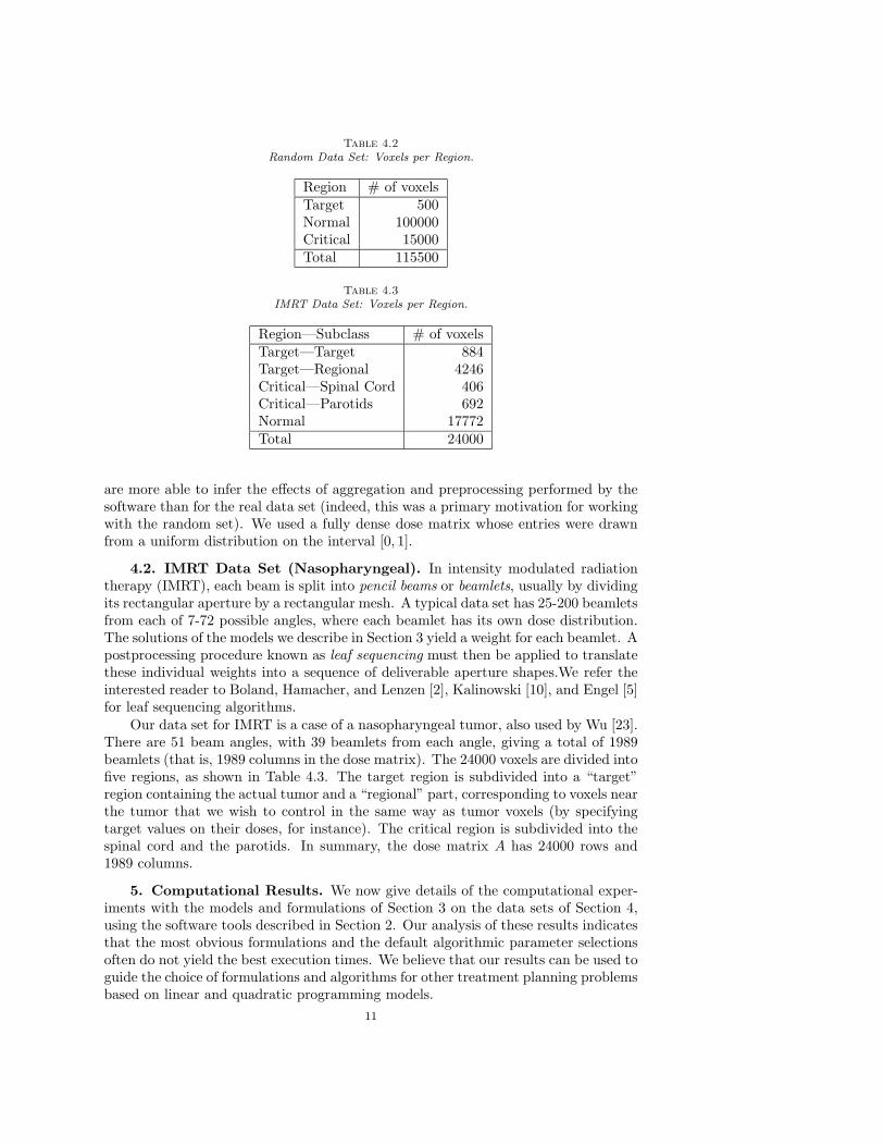
Table 4.2

Random Data Set: Voxels per Region.

Region # of voxelsTarget 500Normal 100000Critical 15000Total 115500

Table 4.3

IMRT Data Set: Voxels per Region.

Region—Subclass # of voxelsTarget—Target 884Target—Regional 4246Critical—Spinal Cord 406Critical—Parotids 692Normal 17772Total 24000

are more able to infer the effects of aggregation and preprocessing performed by thesoftware than for the real data set (indeed, this was a primary motivation for workingwith the random set). We used a fully dense dose matrix whose entries were drawnfrom a uniform distribution on the interval [0, 1].

4.2. IMRT Data Set (Nasopharyngeal). In intensity modulated radiationtherapy (IMRT), each beam is split into pencil beams or beamlets, usually by dividingits rectangular aperture by a rectangular mesh. A typical data set has 25-200 beamletsfrom each of 7-72 possible angles, where each beamlet has its own dose distribution.The solutions of the models we describe in Section 3 yield a weight for each beamlet. Apostprocessing procedure known as leaf sequencing must then be applied to translatethese individual weights into a sequence of deliverable aperture shapes.We refer theinterested reader to Boland, Hamacher, and Lenzen [2], Kalinowski [10], and Engel [5]for leaf sequencing algorithms.

Our data set for IMRT is a case of a nasopharyngeal tumor, also used by Wu [23].There are 51 beam angles, with 39 beamlets from each angle, giving a total of 1989beamlets (that is, 1989 columns in the dose matrix). The 24000 voxels are divided intofive regions, as shown in Table 4.3. The target region is subdivided into a “target”region containing the actual tumor and a “regional” part, corresponding to voxels nearthe tumor that we wish to control in the same way as tumor voxels (by specifyingtarget values on their doses, for instance). The critical region is subdivided into thespinal cord and the parotids. In summary, the dose matrix A has 24000 rows and1989 columns.

5. Computational Results. We now give details of the computational exper-iments with the models and formulations of Section 3 on the data sets of Section 4,using the software tools described in Section 2. Our analysis of these results indicatesthat the most obvious formulations and the default algorithmic parameter selectionsoften do not yield the best execution times. We believe that our results can be used toguide the choice of formulations and algorithms for other treatment planning problemsbased on linear and quadratic programming models.

11

We have split this section into subsections for each type of model. For eachmodel we discuss separately the results for conformal radiotherapy and IMRT. Theexperiments are based on comparisons of the solve time for each model by usingdifferent formulations and options in CPLEX. We apply both simplex and interiorpoint method to models I, II, and III in turn; to the full-size and reduced variants;and to the primal and dual formulations of each model. Model IV is only solved withthe interior point method, for the reduced forms of the problems.

In all the following experiments, we set the normal voxel penalty vector cN toe = (1, 1, . . . , 1)T . For the pancreatic data set, we used xL

T= 0.95e and xU

T= 1.07e as

bounds on the target voxel dose, and xLT

= 50e and xUT

= 75e for the IMRT data set.(These bounds were chosen to produce solutions with reasonable characteristics.) Thelower and upper bound for the random data were generated by setting every thirdelement of w to 1 and x = AT w. Then

xLT

= 0.65 ∗

∑|T |i=1 xi

|T |and xU

T= 1.35 ∗

∑|T |i=1 xi

|T |. (5.1)

A similar technique was used to generate the threshold value b:

x = AT w, b =

|C|∑

i=1

xi/|C|

e. (5.2)

For model III, the penalty vector cT for the deviation from the desired dose is set toe. In model IV we used cT = 2e.

All experiments were performed on a computer running Redhat Linux 7.2 with a1.6GHz Intel Pentium 4 processor with cache size 256 KB and total memory 1 GB.

5.1. Model I Results. The parameter specific to model I is the upper boundvector xU

Non the normal voxel dose. To choose an appropriate value for this bound,

we first solved the problem without these bounds. For the pancreatic data set, thehighest doses to a voxel in each critical region (measured in relative units) were: .461(spinal cord), .915 (liver), .111 (left kidney) and .612 (right kidney) (see Table 4.1 fora summary of the voxel distribution for this data set). To ensure that the boundswere active for at least some voxels, we set the components of the bound vectors forthese different regions as follows: 1.07 (normal and target regions), .40 (spinal cord),.10 (left kidney), .55 (right kidney). For the IMRT data set, the non-bounded solutionhad maximum doses to the parotids of 56.15 Gy (where “Gy” denotes “Grey”, theunit of radiation) and to the spinal cord of 14.13 Gy. We set the bounds as follows:75 Gy (target and normal tissue), 50 Gy (parotids), and 10 Gy (spinal cord).

At the solution, the pancreatic data set yielded only 5 normal voxels at theirupper bound. As noted earlier, this model solves in a fraction of a second if theseupper bounds are removed. Hence, although the upper bounds have little effect on theactual solution of the treatment planning problem in this case, they greatly increasethe time required to solve it. The IMRT data set yields a solution with only 10 normalvoxels at their upper bound. For the IMRT data, removal of the normal voxel boundsimproves the solution time considerably, but not by as much as for the conformalproblem. (The fastest solution time for an unbounded model is about a factor-of-2improvement on the fastest solution times reported below.) Because the dose matrixfor this data set is large and sparse, the linear program is nontrivial even when thenormal voxel bounds are not present in the problem.

12

Table 5.1

Model I Problem Sizes and Effects of Preprocessing.

Before presolve After presolve Avg. presolveData Formulation Rows Columns Rows Columns time (sec)Conf. Full Primal 801815 801851 222690 222726 13.4Conf. Full Dual 801851 1025785 222726 446660 13.8Conf. Red. Primal 239058 1281 72496 1280 1.9Conf. Red. Dual 37 819426 36 73740 4.1IMRT Full Primal 23999 25604 16260 17435 3.2IMRT Full Dual 25174 45820 17435 37651 3.8IMRT Red. Primal 16263 6736 16224 6305 2.7IMRT Red. Dual 1606 29131 1175 21354 4.0

5.1.1. Presolving. The dimensions of the formulations before and after pre-solving are shown in Table 5.1. The first line shows that the number of rows in theformulation (3.1) for the Pancreatic data set is approximately equal to the total num-ber of voxels (see Table 4.1), while the number of columns exceeds this by 36, whichis the number of components in w. Presolving eliminates all those rows and columnscorresponding to components of xN that are intersected by none of the 36 beams(and therefore yield a zero row in the matrix AN ). It also eliminates other rows andcolumns using other techniques. The dual formulation contains approximately twiceas many variables after presolving (see the second line of Table 5.1) because thereare two dual variables µN and µB corresponding to the normal voxels. The reducedprimal form (3.2) (line 3 of the table) initially contains only as many rows as thereare target voxels and normal voxels intersected by the beams; the zero rows of AN

are eliminated by GAMS prior to calling CPLEX. The number of columns equals thenumber of target voxels in xT plus the number of beam weights. General presolvingtechniques reduce the number of rows by a factor of 3. The reduced dual formulation(3.4) (line 4 of the table) has only as many rows as there are beams. The numberof columns is initially the number of normal voxels plus twice the number of targetvoxels, but presolving reduces this number by more than a factor of 10.

Lines 5-8 of Table 5.1 give results for the IMRT data set. Explanations of theproblem dimensions before and after presolving are similar to the pancreatic dataset, though the presolving reductions are less dramatic because almost all voxels areintersected by at least one of the beams. The reduction in line 8 comes from the factthat 1605 beams intersect any voxel, whereas only 1175 of these beams intersect atarget voxel. The remaining beams correspond to zero rows in AT

T , which are theneliminated in the preprocessing of the constraint (3.4b).

5.1.2. Conformal Data Set: Pancreatic. Results for CPLEX simplex codeson the Pancreatic data set are shown in Table 5.2. We start by explaining the structureof the table. It consists of two groups of nine lines each. The first group containsresults for the full-size primal formulation (3.1) (columns 4 and 5) and the reducedprimal formulation (3.2) (columns 6 and 7), while the second group of lines containsresults for the formulation (3.1) with the predual option set (columns 4 and 5) andthe reduced dual formulation (3.4) (columns 6 and 7). Within each group, the firstfour lines represent results for the dual simplex method with four different pivot rules(standard dual pricing, steepest-edge, steepest-edge with slacks, and steepest-edgewith unit initial norms), and the last five give results for the primal simplex methodwith five different pivot rules (reduced-cost pricing, hybrid reduced-cost and devexpricing, devex, steepest-edge, and steepest-edge with slacks). For each combinationof parameter setting, formulation, algorithm, and pivot rule, both the execution time

13

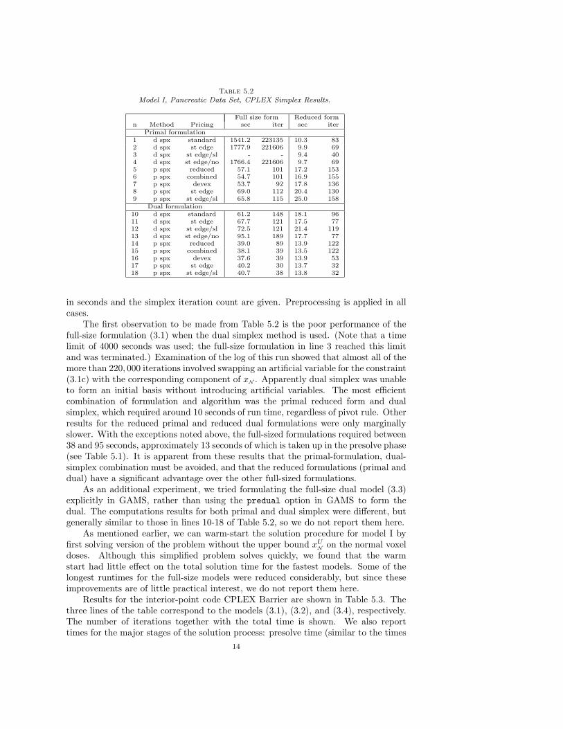
Table 5.2

Model I, Pancreatic Data Set, CPLEX Simplex Results.

Full size form Reduced formn Method Pricing sec iter sec iter

Primal formulation1 d spx standard 1541.2 223135 10.3 832 d spx st edge 1777.9 221606 9.9 693 d spx st edge/sl - - 9.4 404 d spx st edge/no 1766.4 221606 9.7 695 p spx reduced 57.1 101 17.2 1536 p spx combined 54.7 101 16.9 1557 p spx devex 53.7 92 17.8 1368 p spx st edge 69.0 112 20.4 1309 p spx st edge/sl 65.8 115 25.0 158

Dual formulation10 d spx standard 61.2 148 18.1 9611 d spx st edge 67.7 121 17.5 7712 d spx st edge/sl 72.5 121 21.4 11913 d spx st edge/no 95.1 189 17.7 7714 p spx reduced 39.0 89 13.9 12215 p spx combined 38.1 39 13.5 12216 p spx devex 37.6 39 13.9 5317 p spx st edge 40.2 30 13.7 3218 p spx st edge/sl 40.7 38 13.8 32

in seconds and the simplex iteration count are given. Preprocessing is applied in allcases.

The first observation to be made from Table 5.2 is the poor performance of thefull-size formulation (3.1) when the dual simplex method is used. (Note that a timelimit of 4000 seconds was used; the full-size formulation in line 3 reached this limitand was terminated.) Examination of the log of this run showed that almost all of themore than 220, 000 iterations involved swapping an artificial variable for the constraint(3.1c) with the corresponding component of xN . Apparently dual simplex was unableto form an initial basis without introducing artificial variables. The most efficientcombination of formulation and algorithm was the primal reduced form and dualsimplex, which required around 10 seconds of run time, regardless of pivot rule. Otherresults for the reduced primal and reduced dual formulations were only marginallyslower. With the exceptions noted above, the full-sized formulations required between38 and 95 seconds, approximately 13 seconds of which is taken up in the presolve phase(see Table 5.1). It is apparent from these results that the primal-formulation, dual-simplex combination must be avoided, and that the reduced formulations (primal anddual) have a significant advantage over the other full-sized formulations.

As an additional experiment, we tried formulating the full-size dual model (3.3)explicitly in GAMS, rather than using the predual option in GAMS to form thedual. The computations results for both primal and dual simplex were different, butgenerally similar to those in lines 10-18 of Table 5.2, so we do not report them here.

As mentioned earlier, we can warm-start the solution procedure for model I byfirst solving version of the problem without the upper bound xU

Non the normal voxel

doses. Although this simplified problem solves quickly, we found that the warmstart had little effect on the total solution time for the fastest models. Some of thelongest runtimes for the full-size models were reduced considerably, but since theseimprovements are of little practical interest, we do not report them here.

Results for the interior-point code CPLEX Barrier are shown in Table 5.3. Thethree lines of the table correspond to the models (3.1), (3.2), and (3.4), respectively.The number of iterations together with the total time is shown. We also reporttimes for the major stages of the solution process: presolve time (similar to the times

14

Table 5.3

Model I, Pancreatic Data Set, CPLEX Barrier Results.

Formulation iter sec presolve barrier crossoverFull size 75 133.3 14.1 93.3 9.7

Reduced primal 23 20.2 1.9 11.8 3.6Reduced dual 37 26.5 4.1 13.0 1.1

reported in Table 5.1), time for the interior-point algorithm, and time required in the“crossover” phase in which a simplex-like method is used to move the interior-pointsolution to a vertex of the feasible region.

The total time required by the reduced primal and reduced dual formulations(lines 2 and 3 of the table) is 20 and 26 seconds, respectively—competitive with thebest simplex run times from Table 5.2. The full-sized primal formulation requiredconsiderably more iterations (75) and about six times more CPU time. The poorperformance of the full-sized variant is due to the 13 seconds of presolving time andthe fact that the symmetric-positive-definite matrix to be factored at each iterationhas three times as many rows as in the reduced primal case and approximately twiceas many nonzeros in the Cholesky factor. (This matrix has the form ADAT , whereA is the constraint matrix and D is a diagonal scaling matrix.) In both the full-sizedand reduced primal case, the factorization routine correctly detected that 36 columnsin the constraint matrix (specifically, the columns corresponding to w) were dense,and it handled them accordingly. In the reduced dual case, the matrix to be factoredat each interior-point iteration has just 36 rows, However, formation of this matrixADAT is expensive, since A has many columns.

Table 5.4

Model I, IMRT Data Set, CPLEX Simplex Results.

Full size form Reduced formn Method Pricing sec iter sec iter

Primal formulation1 d spx standard 2046 67091 132 140082 d spx st edge 2826 37400 34 15983 d spx st edge/sl 2579 23034 63 15704 d spx st edge/no - - 35 15985 p spx reduced 153 12933 182 160976 p spx combined 153 12933 179 160977 p spx devex 89 11262 98 128738 p spx st edge 209 5407 176 46289 p spx st edge/sl 208 5590 174 4628

Dual formulation10 d spx standard 257 12382 418 2634111 d spx st edge 498 7124 108 591812 d spx st edge/sl 441 6282 317 717413 d spx st edge/no 663 9177 107 591814 p spx reduced 53 5992 30 658615 p spx combined 40 2596 30 658616 p spx devex 40 2596 48 281617 p spx st edge 49 1048 46 119218 p spx st edge/sl 90 2510 46 1192

5.1.3. IMRT Data Set. Results for the CPLEX Simplex codes on the IMRTdata set are shown in Table 5.4. As for the conformal model, the worst performance isturned in by the dual simplex method on the full-size formulation (3.1). Dual simplexwith dual-steepest-norm pricing, reported on line 4 of the table, reaches the runtimelimit of 4000 seconds. Remarkably, this happens to be the default combination ofalgorithm/parameter chosen by GAMS/CPLEX when run without an option file.

15

This observation suggests that it is crucial to make explicit choices of algorithm andparameter for these models, and not to rely on the default choices of the modelingsystem and optimization software.

As in the conformal data sets, dual simplex applied to the full-size primal modelsspends many iterations swapping artificial variables for the constraint (3.1c) with thecorresponding component of xN . Since this data set is so different in nature from theconformal data sets (the dose matrix is sparse with 1175 columns, instead of densewith 36 columns), the more efficient formulations and algorithms do not give quite asdramatic an improvement in runtime as in Table 5.2. However, there is still almosta two-order-of magnitude difference between runtime for the dual simplex/full-sizeprimal models and runtime for the best reduced model.

As in Table 5.2, the fastest runtimes were obtained with the reduced models. Forthe reduced primal model, dual simplex was distinctly faster than primal simplex,while for the reduced dual, primal simplex is better. (These same combinations werethe best for the conformal data set too, but for the IMRT data set the advantages aremore dramatic.) The choice of pivot rule also had a significant effect on runtime insome cases. For the dual simplex algorithm applied to the reduced primal formulation,two of the steepest-edge rules led to a solution being found in around 35 seconds, whilethe standard rule required more than 130 seconds. For primal simplex applied to thereduced dual, on the other hand, standard reduced-cost pricing gave slightly fasterruntimes than devex or steepest-edge rule—about 30 seconds as opposed to 45-50seconds.

Table 5.5

Model I, IMRT Data Set, CPLEX Barrier Results.

Formulation iter sec presolve barrier crossoverFull 3 time limit reached

Red. Primal 0 memory exceededRed. Dual 19 101 4.0 94.8 1.1

Results for CPLEX Barrier applied to the IMRT data set are shown in Table 5.5.We obtained a solution to just one of the three models with this code: the reduceddual model (3.4). The full-size model (line 1 of the table) performed three interior-point iterations before reaching the time limit of 4000 seconds. After presolving, theproblem had 16,260 rows and 17,345 columns, with 147 columns being designated as“dense” by the linear factorization routine in CPLEX Barrier. This code reportedthat the Cholesky factor of the ADAT matrix required about 1.3 × 108 storage loca-tions and about 1.5× 1012 operations to compute. In the reduced primal formulation(line 2), 150 dense columns were detected, and the estimated storage and computa-tion requirements for the factorization were similar to the full-size case. However,this model terminated with an “out-of-memory” message before performing the firstiteration. The reduced dual formulation solved in about 100 seconds, using 19 iter-ations. Dimensions of the reduced LP were modest (1175 × 21354) as were storageand computation times for the Cholesky factorization (7 × 105 locations and 5 × 108

operations). Given the large number of columns, however, computation of the ADAT

matrix also contributes significantly to the total computation time. We concludethat the interior-point approach applied to the reduced dual formulation is a reason-able approach, requiring about a factor of 3 more in runtime than the best simplexformulations.

16

5.2. Model II Results. Model II, which is targeted at formulations with DVconstraints, contains two important formulation parameters that affect the difficultyof the problem considerably. One is the threshold value b (3.6f). Lower values of b inour model tend to force more voxels to be above-threshold, thus causing more of thecomponents of the excess vector xE to be positive. The second important parameteris cE , the penalties applied to the excess doses. Larger values of the components ofcE tend to force more of the voxels below the threshold. For each of our three datasets, we report on values of these parameters that give a wide range of proportionsof above-threshold voxels, to illustrate the performance of our methods under thesedifferent conditions.

5.2.1. Presolving. The dimensions of our various formulations before and afterpresolving are shown in Table 5.6. The effects of presolving on the random data setare particularly instructive, since elimination of rows and columns for this set aremade possible only by structural considerations and not for any reasons of sparsityin the dose matrices (which are deliberately chosen to be dense). The first row ofTable 5.6 suggests that, prior to presolving, the full primal model contains the vari-ables xN , xE , xT , and w; the critical dose vector xC has apparently been eliminatedby GAMS. Presolving eliminates the xN vector as well, by means of the constraint(3.6c), at a considerable overhead in computation time (approximately 36 seconds).The second row of Table 5.6 indicates that in the dual formulation, the presolvedmodel retains constraints (3.8b) and (3.8f), enforcing (3.8e) as a bound rather thana general constraint. Again, the overhead in computational time is significant. Ourreduced primal formulation (3.7) (line 3 in Table 5.6) appears to be identical to theformulation obtained by presolving the full-sized primal formulation (3.6), while ourreduced dual formulation (line 4) differs from the presolved version of the full dualby the absence of the µT variables by means of (3.8b). As we see below, the compu-tational benefits obtained by performing this additional elimination by hand appearsto be considerable.

Table 5.6

Model II, Problem Sizes and Effects of Preprocessing. (Conformal Therapy Used on Randomand Pancreatic Data.)

Before presolve After presolve Avg. presolveData Formulation Rows Columns Rows Columns time (sec)

Random Full primal 115501 115531 15500 15530 35.8Random Full dual 100531 131501 530 16500 35.9Random Red. primal 15501 15531 15500 15530 0.5Random Red. dual 31 16001 30 16000 0.5

Pancreatic Full primal 858373 858409 29464 29500 16.1Pancreatic Full dual 832394 886876 1280 29747 16.2Pancreatic Red. primal 70515 70551 29464 29500 0.6Pancreatic Red. dual 37 71759 36 30708 0.6

IMRT Full primal 24001 25606 6228 7403 3.0IMRT Full dual 24077 35790 6304 16488 3.2IMRT Red. primal 6229 7834 6228 7403 0.9IMRT Red. dual 1204 11359 1175 11358 2.2

Presolving has similar effects on the dimensions for the other two data sets (lines5-12 of Table 5.6), with additional reductions due to sparsity in the dose matrices. Wenote that the computational times for preprocessing the full models are considerablyless than for the random data set, again because of the sparsity of the matricesinvolved.

17

5.2.2. Conformal Data Set: Random. Table 5.7 shows results for CPLEX’ssimplex codes on the random data set, for different values of the parameters b andcE , various formulations, and various pivot rules. We first explain the structure of thetable briefly. It is divided into four groups of seven lines each. The first two groups(lines 1-14) give results for the parameter setting b = 0.8, for which about 53% of thevoxels in the critical region exceed b at the solution. Columns 3-6 contain the resultsobtained by setting cE = e, where e is the vector of all 1s of appropriate dimension,while columns 7-10 are for cE = 8e.

The third and fourth groups (lines 15-28) give results for b = 1.0 (approximately2.5% of voxels over threshold). The first and third groups present results for the fullprimal formulation (3.6) (including presolving) and the reduced primal formulation(3.7). The second and fourth groups give results obtained by the GAMS-constructedfull-size dual formulation (using the predual option), and from the reduced dualformulation (3.9). Note that for each group we also ran experiments using (a) dualsimplex/steepest-edge with unit norms and (b) primal simplex/steepest-edge withslacks. We do not report these results in this table or in Tables 5.9 and 5.11 sincethey add little of interest to our conclusions.

The most striking feature of the results is the wide variation in performancefor different formulations, algorithms, and pivot rules. As seen in columns 3-4 and7-8 of the table, the most “obvious” formulation—the full-size primal model (3.6),with preprocessing—gives inferior performance, even if the best possible pivot rule ischosen, and even if the predual option is used to formulate its dual automatically. Forall parameter settings, the best execution time is obtained by formulating the reduceddual (3.9) by hand, and using primal simplex with the simplest pivot rule (reduced-cost pricing); see row 4, columns 5-6 and 7-8 in the second and fourth groups. For allparameter settings, this strategy led to a runtime of no more than 5 seconds, whileruntimes of more than 10 minutes were observed for other choices of formulation andpivot rule. The number of simplex pivots performed by the optimal strategy in just afew seconds seems remarkable; for example, line 11 shows 14,411 pivots in 3 secondsfor b = 0.8 and cE = e. Closer examination shows that since the constraint matrix hasjust 30 rows, each pivot requires an update of a factorization of a 30× 30 matrix—aninexpensive operation. Moreover, a refactorization of the matrix occurs only aboutonce every 50 iterations. Potentially, the most expensive operation in each simplexiteration is pricing, since there are approximately 16,000 columns in the constraintmatrix. Apparently, the partial pricing strategy used by CPLEX ensures that thepricing operation does not examine this entire matrix at each iteration, so this partof the per-iteration cost is also inexpensive in absolute terms.

Several other general observations about the results of Table 5.7 follow.

• For the primal formulations (the first and third groups of lines), the number ofiterations required by the presolved version of the full model (3.6) is identicalto the number of iterations required by the reduced primal formulation (3.7).This observation confirms that the reductions obtained automatically by thepresolver correspond exactly to the ones we found manually in (3.7), and thatthe initialization of the model was the same in both cases. The additionalcost of 40-50 seconds per instance for the full model arises from the cost ofpreprocessing and the cost of recovering the eliminated variables xN after thesolution has been obtained.

• The use of primal formulations (3.6) or (3.7) is almost uniformly worse thanusing the dual formulation (3.9).

18

Table 5.7

Model II, Random Data Set, CPLEX Simplex Results.

Full size form Reduced form Full size form Reduced formMethod Pricing sec iter sec iter sec iter sec iterPrimal form, b=0.8 cE = e, 53% over threshold cE = 8e, 52.9% over thresholdd spx reduced 102 14569 61 14569 182 15289 141 15289d spx st edge 147 10277 102 10277 182 8845 142 8845d spx st edge/sl 152 8914 112 8914 193 8406 150 8406p spx reduced 465 51989 429 51989 564 60986 516 60986p spx combined 492 59019 439 59019 451 56641 420 56641p spx devex 328 57177 281 57177 356 60457 303 60457p spx st edge 688 51307 647 51307 716 51734 667 51734Dual form, b=0.8 cE = e, 53% over threshold cE = 8e, 52.9% over thresholdd spx reduced 239 22220 136 22315 340 22224 137 22314d spx st edge 237 19764 118 19695 200 19768 118 19696d spx st edge/sl 411 19698 192 20114 330 19701 193 20123p spx reduced 46 16460 3 14411 48 16145 5 14036p spx combined 46 16460 3 14411 48 16145 5 14036p spx devex 134 15380 71 14681 129 11307 106 11019p spx st edge 66 9786 46 8772 116 8659 84 8991

Primal form, b=1.0 cE = e, 2.5% over threshold cE = 8e, 2.5% over thresholdd spx reduced 47 1567 6 1567 50 1303 9 1303d spx st edge 53 798 12 798 55 874 14 874d spx st edge/sl 52 626 11 626 53 602 12 602p spx reduced 524 56502 464 56502 486 53483 440 53483p spx combined 440 57855 396 57855 436 56943 387 56943p spx devex 283 53834 227 53834 270 53711 232 53711p spx st edge 593 47720 542 47720 571 46945 526 46945Dual form, b=1.0 cE = e, 2.5% over threshold cE = 8e, 2.5% over thresholdd spx reduced 54 996 8 1042 54 993 8 1042d spx st edge 53 891 8 1016 53 892 8 1018d spx st edge/sl 57 848 10 884 58 851 10 888p spx reduced 45 3689 2 3874 45 2720 2 2263p spx combined 44 3689 2 3874 44 2720 2 2263p spx devex 45 1493 3 1165 49 1753 8 1561p spx st edge 45 1169 3 791 47 824 5 746

• While the best formulation/algorithm/pivot combination was always reduceddual formulation/primal simplex/reduced-cost pivoting, the difference be-tween this combination and the other reduced dual formulations decreasesmarkedly as the number of above-threshold voxels falls. In the fourth groupof lines, the runtimes are similar for all algorithm/pivot combinations, whilein the second group of lines, variations of more than an order of magnitudecan be observed.

• For the dual formulations (3.8) and (3.9), primal simplex uniformly performsbetter than dual simplex. This is because dual simplex needs to use a phase Iprocedure to find an initial point, whereas an initial point for primal simplexis obvious (from (3.8c)) and no phase I is needed. The problem becomessimpler when b increases, so the importance of phase I iterations decreasesand the run times for dual simplex become more competitive.

• For the reduced primal form (the first and third groups of lines), phase I iter-ations also explain the runtime differences between primal and dual simplex.In these cases, it is primal simplex that requires phase I. For example, in lines4-7 for cE = e the phase I iterations vary from 25408 to 30554 iterations.

• The “combined” pivot rule in primal simplex generally reverted to the reduced-cost rule, with only occasional devex pivots. Thus, runtimes for the combinedrule were almost as good as for the reduced-cost rule.

• There are occasional surprising differences in runtime between similar in-stances. For example, in line 1, the reduced formulation for cE = e performs

19

14,569 iterations in 61 seconds while the reduced formulation for cE = 8eperforms 15,289 iterations in 141 seconds—a considerably slower rate of iter-ations/second. The difference seems due mainly to the lesser number of basisrefactorizations required in the first case (18 factorizations) as compared tothe second case (33 factorizations).

Results for the CPLEX Barrier method for these data sets and parameter choicesare shown in Table 5.8. We consider the same choices of problem parameters as inTable 5.7 (b = 0.8, 1.0 and cE = e, 8e), and the full-size, reduced primal, and reduceddual formulations (3.6), (3.7), and (3.9). Presolving was performed, with the samereductions in dimension as seen in Table 5.6. (The presolve is independent of whetherthe Simplex or Barrier solvers are used.) Similarly to Table 5.3, the columns ofTable 5.8 show the number of interior-point iterations, the total time required, thetime spent in presolving, the time spent in the barrier algorithm itself, and finally thetime required for the crossover phase.

Table 5.8

Model II, Random Data Set, CPLEX Barrier Results.

cE = e cE = 8e

Form. b iter sec pre barr cross iter sec pre barr crossFull size 0.8 21 48.0 35.8 4.6 3.4 18 48.0 35.6 4.1 4.0Full size 1.0 25 48.5 35.6 5.3 3.3 19 47.6 35.7 4.3 3.4R. primal 0.8 21 6.5 0.1 4.6 1.1 18 7.0 0.5 4.1 1.6R. primal 1.0 25 7.5 0.5 5.3 1.0 19 6.5 0.5 4.3 1.0R. dual 0.8 19 4.8 0.5 3.5 0.2 20 5.0 0.5 3.7 0.2R. dual 1.0 15 3.9 0.5 2.6 0.1 16 4.2 0.5 3.0 0.2

We note that for the reduced models, the total CPLEX Barrier runtimes aresimilar to the runtimes for the best variants of CPLEX Simplex—just a few secondsin total. The full size model requires about 40 seconds longer, but the difference isentirely due to the cost of preprocessing and of recovering the eliminated variablesafter solving (the latter is included in “crossover” time). The reduced dual formulationis slightly faster. Note that the matrix to be factored at each iteration of the reduceddual formulation is only 30 × 30 and completely dense, so the row/column orderingis not an issue. For the primal formulations, the matrix is considerably larger, butit has a special structure—a rank-30 update of an extremely sparse matrix—arisingfrom the fact that the dose matrix A has just 30 dense columns. The factorizer inCPLEX is able to detect and exploit this structure, so formation and factorization ofthe linear system at each interior-point iteration does not cost much more than forthe more compact dual formulation.

5.2.3. Conformal Data Set: Pancreatic. Results for the CPLEX Simplexcodes on the pancreatic data set, presented in Table 5.9, showed many of the samepatterns observed in the random data set. We report on two different values of theparameter b (.02 and .21), and two different settings for the penalty vector cE ( eand 8e). These values produced a range in the proportion of above-threshold criticalvoxels from about 5% to about 32%. Unlike the random data set, the penalty vectorhad a considerable effect on the proportion of above-threshold voxels.

Again, we see that the reduced dual formulation (3.9), in conjunction with primalsimplex and reduced-cost pricing, yielded the most effective strategy for solving theproblem. This strategy required less than 10 seconds of runtime for each of the fourparameter combinations tried. As in the random data set, the performance differencebetween this strategy and other strategies based on the dual formulation fades as the

20

Table 5.9

Model II, Pancreatic Data Set, CPLEX Simplex Results.

Full size form Reduced form Full size form Reduced formMethod Pricing sec iter sec iter sec iter sec iterPrimal form, b=0.02 cE = e, 31.9% over threshold cE = 8e, 9.7% over thresholdd spx reduced 300 43809 280 43809 286 33333 248 33333d spx st edge 332 28995 297 28995 256 15053 225 15053d spx st edge/sl 519 28641 498 28641 296 14266 265 14266p spx reduced 305 42005 268 42005 211 32060 179 32060p spx combined 348 60249 315 60249 232 41896 201 41896p spx devex 282 56497 249 56497 178 41774 156 41774p spx st edge 545 36123 495 36123 276 20057 228 20057Dual form, b=0.02 cE = e, 31.9% over threshold cE = 8e, 9.7% over thresholdd spx reduced 212 30943 237 45110 207 30966 233 45090d spx st edge 201 23536 113 23538 201 23638 112 23648d spx st edge/sl 206 17656 96 13479 181 17654 95 13330p spx reduced 52 58002 9 54183 59 50343 7 39549p spx combined 53 58002 9 54183 59 50343 8 39549p spx devex 108 29221 94 29021 169 29302 85 16675p spx st edge 224 41201 108 24909 198 20750 109 13897

Primal form, b=0.21 cE = e, 11.3% over threshold cE = 8e, 5.6% over thresholdd spx reduced 235 32120 207 32120 139 13784 104 13784d spx st edge 213 17799 180 17799 143 8230 110 8230d spx st edge/sl 297 16320 262 16320 177 7919 142 7919p spx reduced 219 27470 186 27470 210 25509 174 25509p spx combined 332 50119 305 50119 226 32673 191 32673p spx devex 335 60427 292 60427 165 32191 132 32191p spx st edge 556 39652 516 39652 302 24329 270 24329Dual form, b=0.21 cE = e, 11.3% over threshold cE = 8e, 5.6% over thresholdd spx reduced 107 12988 68 13550 107 13115 65 13615d spx st edge 109 9998 48 8964 105 10053 46 8937d spx st edge/sl 119 8581 72 8810 120 8657 69 8832p spx reduced 47 29863 6 35187 49 25222 6 24881p spx combined 47 29863 7 35187 49 25222 6 24881p spx devex 86 13245 64 14904 108 13090 45 8115p spx st edge 138 14166 95 12674 125 10144 64 7135

number of above-threshold voxels drops, but the difference is still up to an order ofmagnitude in the fourth group of lines. The reason is probably that there are still5 − 11% of voxels above threshold in this part of the table, whereas for the fourthgroup of lines in Table 5.7, only 2.5% of critical voxels remain above threshold. Notetoo that in Table 5.9, results for even the worst dual formulation cases are better thanthe best cases for the primal formulation.

As for the random data set, the full size model and the reduced primal modelbecame identical after preprocessing, so the number of simplex iterations for thesetwo variants is the same in the first and third groups of lines. The differences in timescan again be accounted for by the cost of presolving and of recovering the eliminatedvariables.

Table 5.10

Model II, Pancreatic Data Set, CPLEX Barrier Results.

cE = e cE = 8e

Form. b iter sec pre barr cross iter sec pre barr crossFull size 0.02 34 47 16.1 6.6 7.2 234 77 16.3 40.1 4.0Full size 0.21 86 52 16.2 14.2 3.9 100 62 16.4 16.4 12.0R. primal 0.02 34 14 0.7 6.6 5.1 234 44 0.7 40.0 1.9R. primal 0.21 86 18 0.6 14.3 1.8 100 28 0.7 16.4 9.8R. dual 0.02 295 38 0.6 35.6 1.1 195 25 0.6 3.6 0.2R. dual 0.21 29 5 0.6 3.5 0.2 75 10 0.6 8.8 0.2

Table 5.10 shows results obtained with CPLEX Barrier on the same four param-eter combinations as reported in Table 5.9. As for the random data set, the results

21

obtained for the full-sized formulation (lines 1-2 of the table) differ from those ob-tained from the reduced primal formulation (lines 3-4) only in the cost of presolvingand recovery of the eliminated variables. We do however see some marked differencewith the random data set (Table 5.8) and also with the IMRT data set (Table 5.12),in that the number of interior-point iterations is unusually large for some parametercombinations—up to 295 iterations, for instance, for the reduced dual formulationapplied to b = 0.02 and cE = e. Still, for all but the latter parameter combination,the reduced dual formulation gave the best solution times. The best CPLEX Barriertimes (obtained for the reduced dual formulation) are generally slower than the bestCPLEX Simplex times, though still much faster than many of non-optimal CPLEXSimplex variants.

In summary, the results for the random and pancreatic data sets suggest thatthe best strategies in general for model II applied to conformal data sets are (i)reduced dual formulation/primal simplex/reduced-cost pivoting; and (ii) reduced dualformulation/interior-point method.

Table 5.11

Model II, IMRT Data Set, CPLEX Simplex Results.

Full size form Reduced form Full size form Reduced formMethod Pricing sec iter sec iter sec iter sec iterPrimal form, b=30 cE = e, 56.4% over threshold cE = 8e, 21% over thresholdd spx reduced 55 7434 48 7318 54 6776 58 7629d spx st edge 26 2366 22 2322 30 2624 25 2559d spx st edge/sl 51 2673 52 2429 56 2907 54 2654p spx reduced 193 36830 186 36830 210 38514 201 38514p spx combined 161 32950 156 32950 181 35766 172 35766p spx devex 161 38741 157 38741 187 44032 183 44032p spx st edge 289 18951 286 18951 259 16988 251 16988Dual form, b=30 cE = e, 56.4% over threshold cE = 8e, 21% over threshold

d spx reduced 313 24980 425 31113 294 21956 398 27814d spx st edge 170 6303 107 6839 171 6281 109 6715d spx st edge/sl 205 6839 207 6931 204 6768 205 6614p spx reduced 61 13666 26 9406 97 21803 28 10028p spx combined 59 9048 27 9406 91 13701 27 10028p spx devex 60 9048 29 3496 90 13701 36 4059p spx st edge 67 3936 45 1961 72 3924 44 1774

Primal form, b=50 cE = e, 12.6% over threshold cE = 8e, 2.9% over thresholdd spx reduced 48 6949 40 6366 35 4404 27 3980d spx st edge 17 1387 17 1964 18 1522 14 1462d spx st edge/sl 34 1776 39 2046 32 1589 32 1660p spx reduced 186 35700 181 35700 152 29009 151 29009p spx combined 156 31489 151 31489 136 26565 132 26565p spx devex 155 38051 150 38051 149 35994 145 35994p spx st edge 302 20139 299 20139 222 14582 216 14582Dual form, b=50 cE = e, 12.6% over threshold cE = 8e, 2.9% over threshold

d spx reduced 216 19058 277 22245 216 19368 277 23015d spx st edge 176 6688 52 4241 164 6230 53 4496d spx st edge/sl 179 6064 157 5501 188 6380 160 5658p spx reduced 31 6319 22 7379 35 7106 20 6522p spx combined 25 3021 22 7379 27 3503 21 6522p spx devex 24 3021 24 2864 27 3503 24 2551p spx st edge 35 1723 37 1575 37 1796 33 1304

5.2.4. IMRT Data Set. The performance results obtained from the IMRTdata are quite different in character from those of the conformal data sets. Again,we tried four parameter combinations—two values of b and two values of cE , resultingin between 3% and 56% of critical voxels being above-threshold at the solution. Asin the pancreatic data set (but unlike the random data set), the choice of cE made asignificant difference in the number of over-threshold voxels.

Table 5.11 shows performance results for CPLEX Simplex. While the best strat-

22

egy for the conformal data sets—reduced dual formulation/primal simplex/reduced-cost pivoting—remains a good choice for the IMRT data, other strategies are as goodor better. For any choice of pivot rule, the use of reduced dual formulation with primalsimplex gives good results; see lines 11-14 and 25-28 of the table. More surprisingly,the use of a primal formulation in conjunction with dual simplex gives competitiveand even superior performance; see lines 1-3 and 15-17.

Note for this data set that the times per iteration have generally increased overthose reported in Tables 5.7 and 5.9, since we are dealing with sparse factorizationsof much larger basis matrices than in these conformal data sets.

Interestingly, for the CPLEX Simplex method applied to Model II for all threedata sets (Tables 5.7, 5.9, and 5.11), the solution time for the best cases is not sensitiveto changes in the parameters b and cE . On the other hand, the solution time for thepoorly performing simplex variants varies greatly. This observation illustrates theimportance of choosing the right combination of method and options.

Note that the proportion over threshold reported in Table 5.11 are obtained fromthe results for the full-sized formulation. In this case (and only this case) we observedthat there were multiple solutions to the problem, which gave rise to slight variationsin the number of voxels above threshold.

Table 5.12

Model II, IMRT Data Set, CPLEX Barrier Results.

cE = e cE = 8e

Form. b iter sec pre barr cross iter sec pre barr crossFull size 30 13 844 3.03 838 2.04 11 730 3.05 724 1.77Full size 50 11 735 3.01 729 1.78 13 849 2.88 843 2.34

Red. primal 30 13 865 0.95 862 1.29 11 745 0.95 742 1.25Red. primal 50 11 745 0.94 742 1.30 13 868 0.94 865 1.60Red. dual 30 15 53 2.20 49 0.64 17 58 2.20 54 0.67Red. dual 50 15 52 2.01 48 0.70 18 60 2.14 57 0.32

Results for CPLEX Barrier applied to the IMRT data set are given in Table 5.12.As in the conformal cases, the full-size formulations (lines 1-2) and the reduced primalformulations (lines 3-4) reduce to the same problem after preprocessing. However,both of these formulations are far less efficient than the reduced dual formulation(lines 5-6), which yields runtimes of between 50 and 65 second on the four parametercombinations. These times are within factor of 3 of the best simplex results fromTable 5.11. The large difference between the performance of the reduced primal andreduced dual models in Table 5.12 can be accounted for by the much greater timeper interior-point iteration associated with the primal formulations. In the primalformulations, the matrix to be factored at each interior-point iteration has dimension6228 and is dense. Although the dose matrix (which forms 1175 columns of theconstraint matrix, is sparse) its outer product with itself is quite dense. The columnsof the dose matrix cannot be extracted and handled separately by the linear algebraroutines, as happens to the 30 or 36 dense columns in the conformal models. In thereduced dual formulation, on the other hand, the dense matrix to be factored at eachiteration has dimension 1175. As can be observed by comparing lines 5-6 of Table 5.12with lines 1-4, the cost of forming and factoring this matrix is more than an order ofmagnitude less than the cost of working with the much larger matrix arising in theprimal formulations.

5.2.5. Sampling from the Critical Structures. In comparing the results formodel I with those for model II, we see that imposition of DV constraints on the critical

23

Table 5.13

Model II, Sampling from the Pancreatic Data Set with Excess Penalty e.

Method Form. Pricing b Sampled Prop sec iterp spx red. pri. devex 0.02 0.125 0.321 10 6569p spx red. pri. devex 0.02 0.250 0.323 12 9877p spx red. pri. devex 0.02 0.500 0.311 68 29160p spx red. pri. devex 0.02 1.000 0.319 245 56497d spx red. pri. st. edge 0.21 0.125 0.156 3 2928d spx red. pri. st. edge 0.21 0.250 0.167 13 7454d spx red. pri. st. edge 0.21 0.500 0.148 45 11309d spx red. pri. st. edge 0.21 1.000 0.113 180 17799p spx red. dual reduced 0.02 0.125 0.321 1 6168p spx red. dual reduced 0.02 0.250 0.323 1 13345p spx red. dual reduced 0.02 0.500 0.311 3 25259p spx red. dual reduced 0.02 1.000 0.319 9 54183p spx red. dual reduced 0.21 0.125 0.156 1 7322p spx red. dual reduced 0.21 0.250 0.167 2 12862p spx red. dual reduced 0.21 0.500 0.148 3 18088p spx red. dual reduced 0.21 1.000 0.113 7 35187

structure voxels makes the linear program considerably harder to solve. Lim et al. [16]showed that a sampling strategy (in which just a subset of critical voxels is includedin the formulation, or adjoining voxels are aggregated into a single larger voxel) hasthe potential to reduce the size and solution time considerably while degrading thequality of the solution only minimally. We used the conformal pancreatic data setto study the effects of these sampling strategies on solve time. We tested only thosemethods and pivot rules that gave the best results in columns 3-6 of Table 5.9 (forwhich the critical voxel weight vector cE is set to e).

Results are shown in Tables 5.13. For each case, we tried sampling four differentfractions of the critical voxels in the constraint (3.6f): 0.125, 0.25, 0.5, and 1.0. (Ofcourse, the fraction 1 is simply the original problem reported in Table 5.9.) Steepest-edge with norms pricing was used in lines 5-8. As each group of four lines in thesetables shows, sampling caused a dramatic reduction in runtime in each case; in fact,the runtime appears to grow superlinearly with the size of the sample fraction.

The third-last column of the tables shows the proportion of critical voxels overthe threshold value. Note that these values fluctuate as the sample size changes.For instance, when b = 0.21, 15.6% are over threshold when a sample fraction of.125 is used, compared to a proportion of 11.3% when the full set of voxels is used(sample fraction 1.0). Not surprisingly, the solution is changing as the sample sizechanges. Since the small-sample formulation is so inexpensive to solve, however, itis cheaper to adjust the parameter b and re-solve this model to achieve the targetproportion-over-threshold value than to work with the full model.

5.3. Model III results. Most parameters for model III have already appearedin earlier models, and the same values are used in the experiments reported in thissection. The exception is the desired dose d for the tumor voxels. For the randomdata and the pancreatic data, we set d = 1.0. For the IMRT data, the desired dose isbased on the sets shown in Table 4.3. The set “Regional” has d = 60.0 while “Target”has d = 70.0.

Dimensions of the problems and formulations before and after preprocessing areshown in Table 5.14. Note here that the preprocessor was able to find the same reduc-tions that we applied to obtain the reduced primal and dual models from the full-sizedprimal and dual models; after presolving, the reduced models had the same dimen-sions as the full models. For the IMRT data set, the presolver was able to eliminate

24

Table 5.14

Model III, Problem Sizes and Effect of Preprocessing. (Conformal Therapy Used on Randomand Pancreatic Data.)

Before presolve After presolve Avg. presolveData Formulation Rows Columns Rows Columns time (sec)

Random Full primal 116001 116531 1000 1530 1.9Random Full dual 115531 118001 530 2000 2.0Random Red. primal 1001 1531 1000 1530 0.0Random Red. dual 531 2001 530 2000 0.0

Pancreatic Full primal 819426 820706 2488 3768 3.5Pancreatic Full dual 818218 824402 1280 4976 3.6Pancreatic Red. primal 2489 3769 2488 3768 0.0Pancreatic Red. dual 1281 4977 1280 4976 0.0

IMRT Full primal 29131 35866 10260 16565 1.9IMRT Full dual 25175 49198 6304 19636 2.1IMRT Red. primal 10261 16996 10260 16565 0.4IMRT Red. dual 6306 20521 6304 19636 0.3

approximately 400 variables from the reduced primal model and 900 variables fromthe reduced dual model.

Table 5.15

Model III, Random Data Set, CPLEX Simplex Results.

Full size ReducedForm Method Pricing sec iter sec iterprimal d spx reduced 8.9 672 0.5 704primal d spx st edge 8.4 656 0.5 639primal d spx st edge/sl 8.7 585 0.6 574primal d spx st edge/no 8.2 656 0.5 639primal p spx reduced 9.4 1305 1.2 1305primal p spx combined 8.7 1088 1.1 1088primal p spx devex 9.4 1211 1.3 1211primal p spx st edge 9.5 955 1.2 955primal p spx st edge/sl 8.7 853 1.1 853dual d spx reduced 8.7 197 0.6 197dual d spx st edge 8.7 174 0.6 174dual d spx st edge/sl 8.8 174 0.6 174dual d spx st edge/no 8.8 179 0.6 179dual p spx reduced 8.6 651 0.5 193dual p spx combined 8.2 657 0.5 173dual p spx devex 8.7 657 0.5 173dual p spx st edge 8.5 583 0.5 85dual p spx st edge/sl 8.0 634 0.5 115

5.3.1. Conformal Data Sets. Results for the random data set appear in Ta-ble 5.15 and in the first 3 lines of Table 5.18. From Table 5.15, we see that for thereduced models the simplex method always required less than 2 seconds to solve thismodel, no matter what variant of algorithm and pivot rule is used. When the full-sizemodel is passed to the solver, approximately 8 seconds are required for preprocessing.Although, as noted above, both full-size and reduced models result in the same formu-lation after preprocessing, the iteration counts are sometimes different. This may bedue to the use of different starting points. The barrier method (Table 5.18) also takesapproximately one second, with an additional 8 seconds required for preprocessing ofthe full-size model.

The pancreatic data set also yields very fast solutions times, again less than 2seconds for any simplex variant, with an additional 20 seconds approximately forpreprocessing the full-size model; see Table 5.16. Results for the barrier code areshown in the second section (lines 4-6) of Table 5.18. The primal models (full-sizeand reduced) were not competitive in this case, requiring 12 seconds for the reduced

25

Table 5.16

Model III, Pancreatic Data Set, CPLEX Simplex Results.

Full size form Reduced formForm Method Pricing sec iter sec iterprimal d spx reduced 21.6 2444 0.3 2459primal d spx st edge 21.7 1371 0.6 1339primal d spx st edge/sl 21.8 1391 1.2 1405primal d spx st edge/no 21.2 2179 0.6 2219primal p spx reduced 22.6 1476 1.8 1476primal p spx combined 22.8 1375 1.6 1375primal p spx devex 21.3 754 1.1 754primal p spx st edge 22.8 727 1.8 727primal p spx st edge/sl 24.7 1822 3.6 1822dual d spx reduced 21.5 260 0.6 260dual d spx st edge 21.4 141 0.6 141dual d spx st edge/sl 21.3 128 0.6 128dual d spx st edge/no 21.9 253 0.8 253dual p spx reduced 21.8 2489 0.4 1679dual p spx combined 20.7 2316 0.4 1106dual p spx devex 21.6 2316 0.3 1106dual p spx st edge 20.9 842 0.4 1029dual p spx st edge/sl 21.1 2187 0.4 979

model and 34 seconds for the full-size model. The reason for these poor times wasthe high cost of factoring the coefficient matrix of the linear system to be solved ateach interior-point iteration. This matrix has dimension 2488 and its lower triangularfactor has approximately 7.7 × 105 nonzeros. The dual formulation yielded a matrixwith only 1280 rows, with 4.5 × 103 nonzeros in the L factor. Hence, each interior-point iteration for the reduced dual problem was much less expensive and the coderequired less than 1 second to solve this formulation.

Table 5.17

Model III, IMRT Data Set, CPLEX Simplex Results.

Full size form Reduced formForm Method Pricing sec iter sec iterprimal d spx reduced 215 25768 216 25768primal d spx st edge 120 10545 124 10545primal d spx st edge/sl 176 11314 172 11314primal d spx st edge/no 165 10946 110 10946primal p spx reduced 2795 149734 2838 149734primal p spx combined 1220 63747 1225 63747primal p spx devex 1542 240848 1555 240848primal p spx st edge 1266 76789 1238 76789primal p spx st edge/sl 1908 119596 1924 119596dual d spx reduced 204 14198 226 15797dual d spx st edge 225 9746 211 8431dual d spx st edge/sl 193 8666 181 7134dual d spx st edge/no 279 12473 228 11054dual p spx reduced 161 36914 183 39015dual p spx combined 131 21024 152 20464dual p spx devex 131 21024 151 20464dual p spx st edge 180 13261 264 17376dual p spx st edge/sl 488 35290 459 30681

5.3.2. IMRT. The solution times for the IMRT data set were considerablylonger than for the conformal data sets, due mainly to the considerably larger sizeof these models after preprocessing. Results for the simplex method are shown inTable 5.17. The most obvious feature of these results was the poor performance ofthe primal simplex method on the primal formulation, which yielded run times almostan order of magnitude higher on average than the other formulations and algorithms.The best time was turned in by the dual simplex applied to the reduced primal formu-

26

Table 5.18

Model III, CPLEX Barrier Results.

Data Form. iter sec presolve barrier crossoverRandom Full size 10 9 2.01 0.96 2.67

R. primal 10 1 0.02 0.94 0.02R. dual 16 0 0.02 0.16 0.01

Pancreatic Full size 12 34 3.70 12.66 2.06R. primal 12 12 0.05 12.18 0.09R. dual 18 1 0.06 0.62 0.05

IMRT Full size 10 400 1.88 394.24 2.16R. primal 10 408 0.78 405.00 1.35R. dual 31 88 0.87 83.69 2.99

lation, using the steepest edge/norms pivot rule (110 seconds). However, most otherrun times were within a factor of three of this number. In general, the safest strategy isto use the dual formulation, since all run times for this formulation (with the possibleexception of primal simplex with the steepest edge/slacks rule) were reasonable.

Results for the barrier code applied to this data set are shown in the last threelines of Table 5.18. For the reduced dual formulation, only 88 seconds are required—faster than any simplex variant. The matrix to be factored at each barrier iterationhas dimension 6304 and its lower triangular factor contains about 1.2× 106 nonzeros.For the primal formulation, the lower triangular factor contains more than ten timesas many nonzeros, so even though fewer barrier iterations are required, the total runtime is higher.

It is particularly interesting to compare the relative behavior of models II andIII on all data sets. For the conformal data set, model III is invariably easy to solve,while model II is fast only for some choices of algorithm and pivot rule (though eventhen considerably slower than model III). For the IMRT data set, on the other hand,model III is much more challenging from a computational point of view. Part of theexplanation lies in the dimensions of the problems. For the conformal data sets inmodel II, the number of columns is between 15,000 and 31,000. Even though thenumber of rows is as small as 30 or 36 (for the reduced dual formulations), the largenumber of columns results in many thousands of simplex iterations. Moreover, pricingis more expensive, even when reduced pricing strategies are used. In model III, atmost 5,000 columns appear in the formulations, and the number of simplex iterationsis rarely greater than 1000. For the IMRT data set, on the other hand, the size of themodel III formulations is significantly larger than the model II formulations, and thenumber of simplex iterations is correspondingly larger as well.

5.4. Model IV results. Model IV is closely related to model III, so in thissection we will tend to compare the computational results of these two models ratherthan to evaluate model IV results in absolute terms. Because of the quadratic objec-tive function in model IV, we cannot use CPLEX’s Simplex solver, only the Barriersolver. Since the full-size model results are uniformly slower than those obtained forthe reduced model, we report only the latter here.

We set the Hessian Q to be the identity in these tests. The penalty factor γT wasset to 2 while the normal penalty vector cN was 1e.

Table 5.19 shows the problem sizes before and after presolving for each dataset and formulation. By comparing the reduced primal formulations for model III(3.11) and model IV (3.15) we see that there are |T | fewer constraints in (3.15).There are also |T | fewer variables, because the single violation variable y in model IVreplaces the two variables s and t in model III. The dimensions of the reduced dual

27

Table 5.19

Model IV, Problem Sizes and Effects of Preprocessing.

Data Formulation Before presolve After presolveRows Columns Rows Columns

Random Red. primal 501 531 500 530Random Red. dual 531 2001 530 2000

Pancreatic Red. primal 1245 1281 1244 1280Pancreatic Red. dual 1281 4977 1280 4976

IMRT Red. primal 5131 6736 5130 6305IMRT Red. dual 6306 20521 6304 20520

Table 5.20

Model IV, CPLEX Barrier Results.

Data set Formulation sec iterRandom Red. primal 1.3 10

Red. primal 1.3 10Red. primal 1.2 10Red. dual 0.5 18Red. dual 0.5 18Red. dual 0.5 17

Pancreatic Red. primal 11.8 12Red. dual 0.9 22

IMRT Red. primal 326 8Red. dual 47 13

models (3.13), (3.16) are identical, as the variable µT in model III is replaced by yin model IV. The preprocessor had essentially no effect in these cases; many of thepreprocessing techniques that can be used for linear programs cannot be applied toquadratic programs.

Table 5.20 shows the results for all data sets using model IV. For the randomdata set, the barrier method converges in 10-18 iterations, and the runtimes are allless than 2 seconds. By comparing with Tables 5.15 and 5.18, we see that model IVappears to be just as easy to solve as model III for this data set.

For the pancreatic data set, the reduced primal model required almost 12 secondsto solve, while the reduced dual model required less than one second. Both times weresimilar to the times required for the corresponding model III formulations reported inTable 5.18. Again, introduction of the quadratic term in model IV does not appearto have made the problem more difficult to solve than model III.

For the IMRT data set (the last two lines of Table 5.20), the reduced dual modelgave the shorter run time; in fact, the time required was only about half of thecorresponding model III formulation (see the last line of Table 5.18) and more thana factor of three faster than the best results for the simplex method on model III(see Table 5.17). This exceptionally good result is due in part to the small numberof interior-point iterations required—only 13, as opposed to 31 for the correspondingmodel III result. (Since the number of interior-point iterations required for a givenproblem is hard to predict or explain in general, we do not speculate on the reasonsfor this improvement here.) Similarly to the results for the conformal-pancreatic dataset, the reduced primal form is much slower to solve than the reduced dual form.

The key observations to be made regarding model IV are as follows. First, despitebeing a quadratic programming model rather than model III’s linear program, itappears to be no more difficult to solve. Second, the reduced dual formulation, whilea less obvious way to pose the problem than the reduced primal formulation, givesvastly better computational results.

28

6. Conclusions. We have performed an extensive computational study of thelinear and quadratic programs that arise in treatment planning problems. Our mostimportant conclusions are that the choice of formulation, algorithm, and pivot rule canbe crucial to the efficiency of the solution procedure, and that the “default” choicesare sometimes unacceptable. We also noted that interior-point methods are oftena good choice, and that quadratic programming formulations can be solved (usinginterior-point methods) as fast or faster than the corresponding linear programmingformulations.

It is important to note that solution of linear programs such as those describedhere represents only a part of the computational and human effort required in thetreatment planning process. Calculation of the dose matrices and the cost of settingthe model up in GAMS are significant. Moreover, enhancements of the models thatrequire the introduction of binary or integer variables (such as limits on the number ofbeams or directions that can be used in the treatment plan) open up a new collectionof algorithmic and computational issues.

Acknowledgments. We thank our colleagues Steven Dirkse, Michael Ferris,and Jin-Ho Lim for their invaluable advice and help with many aspects of this study.This work was supported in part by National Science Foundation Grants #0196485,#0296033, #0127857, #0113051, #0330538, and #0427689.

REFERENCES

[1] G.K. Bahr, J.G. Kereiakes, H. Horwitz, R. Finney, J. Galvin, and K. Goode. The methodof linear programming applied to radiation treatment planning. Radiology, 91:686–693,October 1968.

[2] N. Boland, H. W. Hamacher, and F. Lenzen. Minimizing beam-on time in cancer radiationtreatment using multileaf collimators. Networks, 43(4):226–240, 2004.

[3] A. Brooke, D. Kendrick, A. Meeraus, and R. Raman. GAMS: A User’s Guide. GAMS Devel-opment Corporation, Washington DC, 1998. http://www.gams.com.

[4] G. B. Dantzig. Linear Programming and Extensions. Princeton University Press, Princeton,New Jersey, 1963.

[5] K. Engel. A new algorithm for optimal multileaf collimator field segmentation. Technicalreport, Universitat Rostock, 2002. To appear in Discrete Applied Mathematics.

[6] J. Forrest and D. Goldfarb. Steepest-edge simplex algorithms for linear programming. Mathe-matical programming, 57:341–374, 1992.

[7] http://www.gams.com/contrib/qpwrap/qpwrap.htm.[8] P. M. J. Harris. Pivot selection methods of the Devex LP code. Mathematical programming,

5:1–28, 1973.[9] L. Hodes. Semiautomatic optimization of external beam radiation treatment planning. Radi-

ology, 110:191–196, January 1974.[10] T. Kalinowski. A duality based algorithm for multileaf collimator field segmentation with

interleaf collison constraint. Technical report, Universitat Rostock, 2003. To appear inDiscrete Applied Mathematics.

[11] M. Langer, R. Brown, M. Urie, J. Leong, M. Stracher, and J. Shapiro. Large scale optimizationof beam weights under dose-volume restrictions. Int. J. Radiation Oncol. Biol. Phys.,18(4):887–893, April 1990.

[12] M. Langer and J. Leong. Optimization of beam weights under dose-volume restrictions. Int.J. Radiation Oncol. Biol. Phys., 13(8):1255–1260, August 1987.

[13] M. Langer, S. Morrill, R. Brown, O. Lee, and R. Lane. A comparison of mixed integer pro-gramming and fast simulated annealing for optimizing beam weights in radiation therapy.Medical Physics, 23(6):957–964, 1996.

[14] E. K. Lee, T. Fox, and I. Crocker. Integer programming applied to intensity-modulated radia-tion therapy treatment planning. Annals of Operations Research, 119:165–181, 2003.

[15] J. Lim. Optimization in radiation treatment planning. PhD thesis, Industrial EngineeringDepartment, University of Wisconsin-Madison, 2002.

[16] J. Lim, M. C. Ferris, S. J. Wright, D. M. Shepard, and M. A. Earl. An optimization framework

29

for conformal radiation treatment planning. Technical report, University of Wisconsin-Madison, 2002.

[17] S.M. Morrill, I.I. Rosen, R.G. Lane, and J.A. Belli. The influence of dose constraint pointplacement on optimized radiation therapy treatment planning. Int. J. Radiation Oncol.Biol. Phys., 19(1):129–141, July 1990.

[18] F. Preciado-Walters, R. Rardin, M. Langer, and V. Thai. A coupled column generation, mixedinteger approach to optimal planning of intensity modulated radiation therapy for cancer.Mathematical Programming, 101(2):319–338, 2004.

[19] I. I. Rosen, R. G. Lane, S. M. Morrill, and J. A. Belli. Treatment plan optimization using linearprogramming. Medical Physics, 18(2):141–152, 1991.

[20] D. M. Shepard. Private communication.[21] D. M. Shepard, M. C. Ferris, G. H. Olivera, and T. R. Mackie. Optimizing the delivery of

radiation therapy to cancer patients. SIAM Review, 41(4):721–744, 1999.[22] D. Sonderman and P. G. Abrahamson. Radiotherapy treatment design using mathematical

programming models. Operations Research, 33(4):705–725, 1985.[23] C. Wu. Treatment planning in adaptive radiotherapy. PhD thesis, Medical Physics Department,

University of Wisconsin-Madison, 2002.

30