New compact linear programming formulations for … · New compact linear programming formulations...
40
New compact linear programming formulations for choice network revenue management Sumit Kunnumkal * Kalyan Talluri † November 21, 2014 Abstract The choice network revenue management model incorporates customer purchase behavior as a function of the offered products, and is the appropriate model for airline and hotel network revenue management, dynamic sales of bundles, and dynamic assortment optimization. The op- timization problem is a stochastic dynamic program and is intractable. A certainty-equivalence relaxation of the dynamic program, called the choice deterministic linear program (CDLP ) is usually used to generate dynamic controls. Recently a compact linear programming formula- tion of CDLP for the multinomial-logit (MNL) model of customer choice with non-overlapping consideration sets has been proposed. Our objective is to obtain a tighter bound than CDLP while retaining the appealing properties of a linear programming representation. To this end, it is natural to consider the affine relaxation of the dynamic program. We first show that the affine relaxation is NP-complete even for a single-segment MNL model. Nevertheless, by analyzing the affine relaxation we derive new linear programs that approximate the dynamic programming value function better than CDLP , provably between the CDLP value and the affine relaxation, and often coming close to the latter in our numerical experiments. We give extensions to the case with multiple customer segments and nested-logit model of choice. Finally we perform extensive numerical comparisons on the various bounds to evaluate their performance. 1 Introduction and literature review Revenue management is the control of the sale of a limited quantity of a resource (hotel rooms for a night, airline seats, advertising slots etc.) to a heterogenous population with different valuations for a unit of the resource. The resource is perishable, and for simplicity sake, we assume that it perishes at a fixed point of time in the future. The firm has to decide what products to offer (at a given price for each product), the tradeoff being selling too much at too low a price early and running out of capacity, or, rejecting too many low-valuation customers and ending up with excess unsold inventory. In industries such as hotels, advertising and airlines, the products consume bundles of different resources (multi-night stays, bundles of ad slots, multi-leg itineraries) and the decision to accept or reject a particular product at a certain price depends on the future demands and revenues for all the * Indian School of Business, Hyderabad, 500032, India, email: sumit [email protected] † ICREA and Universitat Pompeu Fabra, Ramon Trias Fargas 25-27, 08005 Barcelona, Spain, email: [email protected] 1
Transcript of New compact linear programming formulations for … · New compact linear programming formulations...
New compact linear programming formulations for choice
network revenue management
Sumit Kunnumkal∗ Kalyan Talluri†
November 21, 2014
Abstract
The choice network revenue management model incorporates customer purchase behavior asa function of the offered products, and is the appropriate model for airline and hotel networkrevenue management, dynamic sales of bundles, and dynamic assortment optimization. The op-timization problem is a stochastic dynamic program and is intractable. A certainty-equivalencerelaxation of the dynamic program, called the choice deterministic linear program (CDLP ) isusually used to generate dynamic controls. Recently a compact linear programming formula-tion of CDLP for the multinomial-logit (MNL) model of customer choice with non-overlappingconsideration sets has been proposed. Our objective is to obtain a tighter bound than CDLPwhile retaining the appealing properties of a linear programming representation. To this end, itis natural to consider the affine relaxation of the dynamic program. We first show that the affinerelaxation is NP-complete even for a single-segment MNL model. Nevertheless, by analyzingthe affine relaxation we derive new linear programs that approximate the dynamic programmingvalue function better than CDLP , provably between the CDLP value and the affine relaxation,and often coming close to the latter in our numerical experiments. We give extensions to thecase with multiple customer segments and nested-logit model of choice. Finally we performextensive numerical comparisons on the various bounds to evaluate their performance.
1 Introduction and literature review
Revenue management is the control of the sale of a limited quantity of a resource (hotel rooms for anight, airline seats, advertising slots etc.) to a heterogenous population with different valuations fora unit of the resource. The resource is perishable, and for simplicity sake, we assume that it perishesat a fixed point of time in the future. The firm has to decide what products to offer (at a givenprice for each product), the tradeoff being selling too much at too low a price early and runningout of capacity, or, rejecting too many low-valuation customers and ending up with excess unsoldinventory.
In industries such as hotels, advertising and airlines, the products consume bundles of differentresources (multi-night stays, bundles of ad slots, multi-leg itineraries) and the decision to accept orreject a particular product at a certain price depends on the future demands and revenues for all the
∗Indian School of Business, Hyderabad, 500032, India, email: sumit [email protected]†ICREA and Universitat Pompeu Fabra, Ramon Trias Fargas 25-27, 08005 Barcelona, Spain, email:
1
resources used by the product and indirectly, on all the resources in the network. Network revenuemanagement (network RM) is control based on the demands for the entire network. Chapter 3 ofTalluri and van Ryzin [19] contains all the necessary background on network RM.
RM incorporating more realistic models of customer behavior as customers choosing from setof offered products have recently become popular, initiated in Talluri and van Ryzin [18] for thesingle-resource problem. Bodea, Ferguson, and Garrow [3] for instance use choice data from a largehotel chain and empirically study the suitability of choice models. Vulcano, van Ryzin, and Chaar[22] and Newman, Ferguson, Garrow, and Jacobs [12] and Talluri [16] study estimation of choicemodels from sales data.
The choice network RM problem can be formulated as a dynamic program with exponentiallylarge state and action spaces. Since the dynamic programming formulation is computationally in-tractable, many approximation methods have been proposed starting with Gallego, Iyengar, Phillips,and Dubey [6] and Liu and van Ryzin [9], who formulate the choice deterministic linear program(CDLP ). They show that CDLP gives an upper bound on the value function. Since CDLP has anexponential number of decision variables it has to be solved using column generation. The columngeneration procedure turns out to be tractable for the multinomial-logit (MNL) model of choicewhen the consideration sets of the different customer segments are disjoint ([9]). However, generat-ing the columns is difficult (NP-complete) when the segment consideration sets overlap under theMNL model with just two segments ([4], [14]).
Given the difficulty of solving CDLP , Talluri [17] explores a weaker segment-based determin-istic concave program (SDCP ) formulation. The SDCP formulation is further strengthened byadding equalities called product-cuts in Meissner, Strauss, and Talluri [11]. Strauss and Talluri [15]show that SDCP with the product-cuts added is equivalent to CDLP when the consideration setintersections have a tree structure.
Kunnumkal and Topaloglu [8] and Zhang and Adelman [23] study decomposition procedures andan affine relaxation of the dynamic program. In the same vein, Meissner and Strauss [10] look attime-sensitive bid-price controls based on a decomposition procedure. All these methods yield upperbounds on the value function that are provably tighter than the CDLP upper bound. However theyare not easy to solve, even for a single-segment MNL model of choice.
Recently, Gallego, Ratliff, and Shebalov [7] give a new compact formulation of CDLP called thesales-based linear program (SBLP ) for the case of MNL with non-overlapping segment considera-tion sets. This formulation is very appealing as it is compact—not requiring column or constraintgeneration—and hence scalable to industrial-size problems.
Can we obtain a tighter bound than SBLP while maintaining a compact formulation? To thisend, it is natural to consider the affine relaxation of the dynamic program. Unfortunately, we showthat the affine relaxation is NP-complete even for a single-segment MNL model, possibly markingthe limit of tractability of dynamic programming approximations. Nevertheless, by analyzing theaffine relaxation we derive new linear-programming formulations that yields an upper bound on thedynamic programming value function and are provably tighter than the CDLP bound. Moreover,for the MNL model, our formulations are compact and similar to the one discovered in [7]. Althoughtheoretically weaker than the affine relaxation, we find in our numerical study, that our relaxationsare often close to the affine relaxation upper bound.
To summarize, our contributions in this paper are as follows:
1. We show that the affine relaxation is NP-hard even for a single-segment MNL. Previously there
2
was some hope that CDLP could be improved at least for this simple and widely used choicemodel.
2. We propose new relaxations based on the affine relaxation. This shows that there is some valueand insight possible from formulating and analyzing dynamic programming relaxations—evenif the actual relaxation is difficult we obtain new insights for tractable relaxations. For theMNL model, not only are our relaxations provably tighter than CDLP and tractable, but theyalso can be formulated as compact linear programs. Compact representations are appealingfrom an implementation perspective since it eliminates the need for customized coding in theform of constraint or column generation techniques.
3. We give extensions to multiple segments, nested logit, study alternate relaxations theoreticallyand numerically and analyze the applicability of the product cuts developed in Meissner et al.[11].
4. We develop policies based on the relaxations and perform numerical experiments to study theeffectiveness of the new formulations.
The remainder of the paper is organized as follows: In §2 we describe the network choice RMmodel, the notation, and the basic dynamic program. In §3 we state the CDLP and the affinerelaxation of the dynamic program.Next, in §4 we show that the affine relaxation is NP-hard evenfor single segment MNL and give various relaxations which are tractable and fall in between CDLPand the affine relaxation. §5 discusses extensions to multiple segments and nested logit. §6 containsour computational study using the new formulations.
2 Model and notation
Our model and notation is to a large part based on Liu and van Ryzin [9]. A product is a specificationof a price and the set of resources that it consumes. For example, a product could be an itinerary-fare class combination for an airline network, where an itinerary is a combination of flight legs; in ahotel network, a product would be a multi-night stay for a particular room type at a certain pricepoint. Time is discrete and assumed to consist of τ intervals, indexed by t. The booking horizonbegins at time t = 1 and ends at t = τ ; all the resources perish instantaneously at time τ + 1. Wemake the standard assumption that the time intervals are fine enough so that the probability ofmore than one customer arriving in any single time period is negligible. The underlying networkhas m resources (usually indexed by i) and n products (usually indexed by j), and we refer to theset of all resources as I and the set of all products as J . A product j uses a subset of resourcesIj ⊆ I, and its sale brings in revenue fj . A resource i is used by a subset Ji ⊆ J of products. Aresource i is said to be in product j (i ∈ Ij) if j uses resource i, and conversely we write j ∈ Ji.
The resources used by product j are represented by the 0-1 incidence vector 1[Ij ], which has a1 in the ith position if i ∈ Ij and a 0 otherwise.
We use superscripts on vectors to index the vectors (for example, the resource capacity vectorassociated with time period t would be rt) and subscripts to indicate components (for example, thecapacity on resource i in time period t would be rti). We use 1[·] as the indicator function, 1 if trueand 0 if false.
We let r1 = [r1i ] represent the initial capacity on the resources and rt = [rti ] denote the remainingcapacity on resource i at beginning of time period t. The remaining capacity rti takes values in the
3
set Ri = {0, . . . , r1i } and R =∏iRi represents the state space.
2.1 Demand model
We assume there are L = {1, . . . , L} customer segments, each with distinct purchase behavior. Ineach period a customer from segment l arrives with probability λl so that λ =
∑l λl is the total
arrival rate. Note that conditioned on a customer arrival, λl/λ is the probability that the customerbelongs to segment l.
Each segment l has a consideration set Cl ⊆ J of products that it considers for purchase. Weassume this consideration set is known to the firm (by a previous process of estimation and analysis).The choice probabilities of a segment-l customer are not affected by products not in its considerationset.
In each period the firm offers a subset S of its products for sale, called the offer set. Given anoffer set S, an arriving customer purchases a product j in the set S or decides not to purchase. Theno-purchase option is indexed by 0 and is always present for the customer.
A segment-l customer purchases j ∈ S with given probability P lj(S). This is a set-functiondefined on all subsets of J . For the moment we assume these set functions are given by an oracle;it could conceivably be given by a simple formula such as the multinomial-logit (MNL) model. IfSl = Cl ∩ S note that P lj(S) = P lj(Sl).
Given a customer arrival, and an offer set S, the probability that the firm sells j ∈ S is then givenby Pj(S) =
∑lλl
λ Plj(Sl) and makes no sale with probability P0(S) = 1−
∑j∈S Pj(S). The expected
sales for product j is therefore λPj(S) =∑l λlP
lj(S), while 1 − λ + λP0(S) = 1 −
∑j∈S λPj(S) is
the probability of no sales in a time period. Given an offer set S, Qli(S) =∑j∈Ji
P lj(S) denotes theexpected capacity consumed on resource i conditional on a segment-l customer arrival and Qi(S) =∑lλl
λ Qli(S) denotes the expected capacity consumed on resource i conditional on a customer arrival.
Note that λQi(S) =∑l λlQ
li(S) gives the expected capacity consumed on resource i in a time period.
The revenue functions can be written as Rl(S) =∑j∈Sl
fjPlj(Sl) and R(S) =
∑j∈S fjPj(S).
We write i ∈ IS whenever there is a j ∈ S with i ∈ Ij . We also assume that the arrival ratesand choice probabilities are stationary. This is again for brevity of notation and all of our results gothrough with nonstationary arrival rates and choice probabilities.
2.2 MNL model
Some of the results of this paper apply to general discrete-choice models, but the main new relax-ations apply to the MNL model of choice.1
In the MNL model of choice probabilities, when a subset Sl ⊆ Cl of products are offered by thefirm, a customer in segment l chooses product j ∈ Sl with probability
P lj(Sl) =wlj
1 +∑k∈Sl
wlk,
where wlj is a weight associated with product j. The no-purchase option is indexed 0, and we
1Our results in fact extend unchanged to the slightly more general attraction model of [7].
4
normalize the weights so that the no-purchase weight is 1.0. So if Sl is offered, a customer does notpurchase any of the offered products and leaves the system with a probability P l0(Sl) =
11+
∑k∈Sl
wlk
.
The weight wlj represents the exponential of a utility the customer derives from j as a functionof some attributes of the product (such as price etc.). As we fix all the attributes and our decision ison subsets to offer, we do not delve too much into how the weights are formed. We refer the readerto Ben-Akiva and Lerman [2] for background on this popular model. The firm does not observesegment membership.
The case of non-overlapping consideration sets for the segments is one of the few known caseswhere the CDLP formulation is solvable. This model is often taken as an approximation (fortractability). Under this assumption, the L segments have considerations sets that do not overlap(Cl ∩ Cl′ = ∅, l = l′).
2.3 Choice dynamic program
The dynamic program (DP) to determine optimal controls is as follows. Let Vt(rt) denote the
maximum expected revenue to go, given remaining capacity rt at the beginning of period t. ThenVt(r
t) must satisfy the Bellman equation
Vt(rt) = max
S⊆S(rt)
∑j∈S
λPj(S)[fj + Vt+1
(rt − 1[Ij ]
)]+ [λP0(S) + 1− λ]Vt+1
(rt) , (1)
whereS(r) =
{j |1[i∈Ij ] ≤ ri ∀i
}represents the set of products that can be offered given the capacity vector r. The boundaryconditions are Vτ+1(r) = Vt(0) = 0 for all r and for all t, where 0 is a vector of all zeroes.V DP = V1(r
1) denotes the optimal expected total revenue over the booking horizon, given theinitial capacity vector r1.
2.4 Linear programming formulation of the dynamic program
The value functions can, alternatively, be obtained by solving a linear program; see Zhang andAdelman [23]. The linear programming formulation of the network choice RM DP given below, hasa decision variable for each state vector in each period Vt(r) and is as follows:
V DPLP = minV
V1(r1) (2)
s.t.
(DPLP ) Vt(r) ≥∑j
λPj(S)[fj + Vt+1
(r − 1[Ij ]
)− Vt+1 (r)
]+ Vt+1 (r)
∀ r ∈ R, S ⊆ S(r), t,
with the boundary condition that Vτ+1(·) = 0. Both the dynamic program (1) and linear programDPLP are computationally intractable, but the linear program DPLP turns out to be useful indeveloping value function approximation methods. In the next section, we describe methods toapproximate the value function.
5
3 Approximations and upper bounds
In the following, we outline the two approximations studied in this paper. We first describe thechoice deterministic linear program and then outline the affine relaxation method.
3.1 Choice deterministic linear program (CDLP )
The choice deterministic linear program CDLP proposed in Gallego et al. [6] and Liu and van Ryzin[9] is a certainty-equivalence approximation to (1). We write CDLP in an expanded, redundantway as the following linear program (LP):
V CDLP = maxh
∑t
∑S
λR(S)hS,t
s.t.t∑
k=1
∑S
λQi(S)hS,k ≤ r1i ∀i, t (3)
(CDLP )∑S
hS,t = 1 ∀t (4)
hS,t ≥ 0.
The decision variable hS,t can be interpreted as the frequency with which set S (including the emptyset) is offered at time period t . The first set of constraints ensure that the total expected capacityconsumed on resource i up until time period t does not exceed the available capacity. Note thatsince hS,t ≥ 0, constraints (3) are redundant except for the last time period. Still, this expandedformulation is useful when we compare CDLP with other approximation methods. The second setof constraints states that the sum of the frequencies adds up to 1.
Associating dual variables γ = {γi,t | ∀i, t} with constraints (3) and β = {βt | ∀t} with constraints(4), the dual of CDLP is
V dCDLP = minβ,γ
∑t
βt +∑t
∑i
γi,tr1i
s.t.
(dCDLP ) βt +∑i
(τ∑k=t
γi,k
)λQi(S) ≥ λR(S) ∀t, S (5)
γi,t ≥ 0.
Liu and van Ryzin [9] show that the optimal objective function value of CDLP , V CDLP is anupper bound on V DPLP . Besides giving an upper bound on the value function, CDLP can also beused to construct different heuristic control policies. One idea that is pursued in [23] is to use theoptimal values of the dual variables associated with constraints (3) to come up with a value functionapproximation, and use this approximation in place of the value function in optimality equation (1)to decide on the offer set. Letting γ = {γi,t | ∀i, t} denote the optimal values of the dual variablesassociated with constraints (3), we interpret γi,t as giving the value of an additional unit of capacityon resource i from time period t to t + 1. With this interpretation,
∑τk=t γi,k gives the marginal
value of capacity on resource i at time period t and we approximate the value function as
Vt(r) =∑i
(τ∑k=t
γi,k
)ri. (6)
6
If rt is the vector of remaining resource capacities at time t, we solve the problem
maxS⊆S(rt)
∑j∈S
λPj(S)[fj + Vt+1
(rt − 1[Ij ]
)]+ [λP0(S) + 1− λ] Vt+1
(rt) , (7)
and offer the set which achieves the maximum in the above optimization problem.
Since CDLP has O(2n) decision variables, it has to be solved using column generation. Liuand van Ryzin [9] show that the column generation procedure can be efficiently carried out whenchoice is according to the MNL model and the consideration sets of the different segments do notoverlap. Bront et al. [4] and Rusmevichientong et al. [14] investigate this further and show thatcolumn generation is NP-complete whenever the consideration sets for the segments overlap, for theMNL choice model with just two segments.
3.2 Affine relaxation
The second approximation method we consider is the affine relaxation, where the value function isapproximated as Vt(r) = θt +
∑i Vi,tri. Note that Vi,t can be interpreted as the marginal value of
capacity on resource i at time t. Substituting this value function approximation into the formulationDPLP we get the affine relaxation LP
V AF = minθ,V
θ1 +∑i
Vi,1r1i
s.t.
(AF ) θt +∑i
Vi,tri ≥∑j
λPj(S)
fj − ∑i∈Ij
Vi,t+1
+ θt+1 +∑i
Vi,t+1ri
∀ r ∈ R, S ⊆ S(r), t,θt ≥ 0, Vi,t ≥ 0,
with the boundary conditions θτ+1 = 0, Vi,τ+1 = 0. Zhang and Adelman [23] show that the optimalobjective function value V AF is an upper bound on V DPLP and that there exists an optimal solution(θ, V ) of AF that satisfies Vi,t − Vi,t+1 ≥ 0 for all i and t.
The number of decision variables in AF is manageable, but the number of constraints is ofthe order of |R|2nτ . Vossen and Zhang [21] use Dantzig-Wolfe decomposition to derive a reducedformulation of AF , where the number of constraints is of the order of 2nτ .
We give an alternative, simpler proof of the reduction. We begin by making a change of variables.Letting βt = θt − θt+1, and γi,t = Vi,t − Vi,t+1, we can write AF equivalently as
minβ,γ
∑t
βt +∑t
∑i
γi,tr1i
s.t. βt +∑i
γi,tri +∑j
λPj(S)
∑i∈Ij
τ∑k=t+1
γi,k
− fj
≥ 0 ∀r ∈ R, S ⊆ S(r), t (8)
γi,t ≥ 0,
where we use the fact that Vi,t =∑τk=t γi,k and so
∑τk=t γi,k can be interpreted as the marginal
value of capacity on resource i at time t. Note that the nonnegativity constraint on γi,t is without
7
loss of generality, since there exists an optimal solution to AF that satisfies Vi,t − Vi,t+1 ≥ 0. Now,constraints (8) can be written as
minr∈R,S⊆S(r)
βt +∑i
γi,tri +∑j
λPj(S)
∑i∈Ij
τ∑k=t+1
γi,k
− fj
≥ 0 (9)
for all t. Since γi,t ≥ 0, the coefficient of ri in the minimization problem (9) is nonnegative, and wecan assume ri ∈ {0, 1} in the minimization (as larger values of ri would be redundant in S ⊆ S(r)and would only increase the objective value). Moreover, since γi,t ≥ 0, for any set S, we have ri = 0for i ∈ IS . On the other hand, feasibility requires we have ri = 1 for i ∈ IS . Therefore, (9) can bewritten as
minS
βt +∑i
1[i∈IS ]γi,t +∑j
λPj(S)
∑i∈Ij
τ∑k=t+1
γi,k
− fj
≥ 0. (10)
and we can write AF equivalently as
V RAF = minβ,γ
∑t
βt +∑t
∑i
γi,tr1i
(RAF ) s.t. βt +∑i
1[i∈IS ]γi,t +∑i
[(τ∑
k=t+1
γi,k
)λQi(S)
]≥ λR(S) ∀t, S (11)
γi,t ≥ 0.
Notice that the number of constraints in the reduced formulation RAF is an order of magnitudesmaller than AF . Taking the dual of RAF by associating dual variables hS,t with constraints (11),we get
V dRAF = maxh
∑t
∑S
λR(S)hS,t
s.t.∑S
t−1∑k=1
λQi(S)hS,k + 1[i∈IS ]hS,t ≤ r1i ∀i, t
(dRAF )∑S
hS,t = 1 ∀t
hS,t ≥ 0.
The above arguments imply that
Proposition 1. V AF = V RAF = V dRAF .
In addition to giving an upper bound on the optimal expected total revenue, the affine relaxationcan also used to construct heuristic control policies. Letting (β, γ), with β = {βt | ∀t} and γ ={γi,t | ∀i, t}, denote an optimal solution to RAF , we use
∑τk=t γi,k to approximate the marginal
value of capacity on resource i at time t. We approximate Vt(r) using (6) and solve problem (7)using this value function approximation to decide on the set of products to be offered at time periodt.
In the following, we show how to obtain relaxations that remain tractable for the single-segmentMNL model and that lie in between the CDLP and the AF bounds, by concentrating our attentionon constraint (8).
8
4 Tractable formulations for MNL with a single segment
In this section we restrict our attention to the MNL model with a single segment and develop ourtractable approximations. After some initial preliminary results, we show that the affine relaxationis NP-complete even for the MNL model with a single segment; In contrast CDLP is tractable. Wethen give a series of tractable relaxations that fall in between CDLP and the affine relaxation. In§5 we extend the formulations to generalizations of the single-segment MNL model.
4.1 Preliminaries
In this section we state some known facts and some preliminary results.
Since we restrict attention to the single-segment MNL model, we drop the segment superscriptl and write the weights as wj , and the choice probabilities, expected resource consumptions andexpected revenues as
Pj(S) =1[j∈S]wj
1 +∑j′∈S wj′
Qi(S) =
∑j∈S | i∈Ij
wj
1 +∑j∈S wj
R(S) =
∑j∈S fjwj
1 +∑j∈S wj
.
4.1.1 Compact formulation of CDLP
Gallego et al. [7] give the following equivalent formulation of CDLP for the MNL choice model:
V SBLP = maxx
∑t
∑j
λfjxj,t (12)
s.t.∑t
∑j∈Ji
λxj,t ≤ r1i ∀i (13)
(SBLP ) x0,t +∑j
xj,t = 1 ∀t
xj,twj
− x0,t ≤ 0 ∀j, ∀t
xj,t ≥ 0.
In the above LP, the decision variables xj,t can be viewed as the rate of sales of product j attime period t. The first constraint ensures that the total capacity consumed by the products oneach resource does not exceed the available capacity. The second and third constraints ensure thatthe sales rates are consistent with the MNL choice probabilities. This formulation, referred to asthe sales-based linear program (SBLP ), vastly reduces the complexity of solving CDLP , albeitrestricted to the MNL model.
4.1.2 Affine relaxation for single-segment MNL
Substituting the MNL choice probabilities, expected resource consumptions and expected revenuesinto constraint (11), we obtain
βt + γS,t +∑i
[(τ∑
k=t+1
γi,k
)λ
∑j∈S | i∈Ij
wj
1 +∑j∈S wj
]≥ λ
∑j∈S fjwj
1 +∑j∈S wj
9
whereγS,t =
∑i
1[i∈IS ]γi,t.
Multiplying both sides by the positive quantity 1+∑j∈S wj and simplifying, constraint (11) of RAF
can be equivalently written as
βt ≥ −γS,t
1 +∑j∈S
wj
−∑j∈S
wj
βt + λ
∑i∈Ij
τ∑k=t+1
γi,k
− fj
. (14)
Since the constraint has to be satisfied for every S and t, we have βt ≥ ΠAFt (β, γ) for all t, where
ΠAFt (β, γ) = maxS
−γS,t
1 +∑j∈S
wj
−∑j∈S
wj
βt + λ
∑i∈Ij
τ∑k=t+1
γi,k
− fj
(15)
and the affine relaxation constraint (11) can be written as
βt ≥ ΠAFt (β, γ) ∀t. (16)
4.2 NP-completeness of the affine separation for single-segment MNL
Since RAF has an exponential number of constraints, we have to generate constraints (14) on thefly. Given a set of values (β, γ), the separation problem at time t is to decide if constraint (14) issatisfied for all S, and if not, add the violated constraint to the LP. In other words, the separationproblem at time t involves solving optimization problem (15) and determining if βt ≥ ΠAFt (β, γ).If βt ≥ ΠAFt (β, γ), then constraint (14) is satisfied for all S at time t. Otherwise, the set S whichattains the maximum in problem (15) violates the constraint, and we add the constraint for set S tothe LP. Therefore, solving problem (15) in an efficient manner is key to separating constraints (14)efficiently. Proposition 2 below states that the affine relaxation separation problem for MNL with asingle segment, as given in (14) is NP-complete.
Proposition 2. The following problem is NP-complete:Input: wj ≥ 0, 1 ≥ λ ≥ 0, fj ≥ 0, and values βt and γi,t ≥ 0.Question: Is there a set S that violates (14)?
ProofOur reduction is from the NP-complete maximum edge biclique problem ([13]). We state first thedefinitions and notation in the problem.
The problem is defined on an undirected, bipartite graph G = (V1 ∪ V2, E), with |V2| = m2. A(k1, k2)-biclique is a complete bipartite subgraph of G, i.e., a subgraph consisting of a pair (X,Y )of vertex subsets X ⊆ V1 and Y ⊆ V2, |X| = k1 > 1, |Y | = k2 > 1, such that there exists an edge(x, y) ∈ E, ∀x ∈ X, y ∈ Y . Note that the number of edges in the biclique is k1k2.
Maximum edge biclique problem (MBP)Input: A bipartite graph G = (V1 ∪ V2, E) and a positive integer p.Question: Does G contain a biclique with at least p edges.
Consider the complement bipartite graph G of G defined on the same vertex set as G, wherethere is an edge e = (u, v) in graph G if and only if there is no edge between u and v in G.
10
Define a cover CS ⊆ V2 of a subset S ⊆ V1 in the complement graph G, as CS = {v ∈ V2 | ∃e =(u, v) ∈ G, u ∈ S}. By definition if CS is a cover of some subset S, it means there is no edge fromany u ∈ S to any v ∈ V2\CS in the graph G. Hence, as G is a complement of G, there is an edgefrom every u ∈ S to every v ∈ V \C(S) in G, thus representing a biclique between S and V \C(S) inthe graph G.
Now we set up the reduction for the separation for (14). In equation (14), for each u ∈ V1, we
associate a product j with fj = m2(p+1)p and wj = m2. For each v ∈ V2, we associate a resource i
with weights γi,t =1p and γi,k = 0, k > t. The resource consumptions of the products j are defined
from the graph G: j contains all the i such that there is an edge between the associated nodes inG. We let λ = 1, βt = m2.
We now claim that G has a (k1, k2)-biclique with k1k2 > p if and only if there is a set S thatviolates the inequality (14) for this instance.
With the above values, S ⊆ V1, with |S| = k1, |C(S)| = m2 − k2 violates (14) if and only if
m2 −∑j∈S
(p+1)p (m2)
2
(1 +∑j∈Sm2)
< −∑
i∈C(S)
1
p
or,
m2 −(p+ 1)m2k1
p(
1m2
+ k1
) < − (m2 − k2)
p
or multiplying both sides by the positive number p( 1m2
+ k1),
m2p
(1
m2+ k1
)− (p+ 1)m2k1 < −(m2 − k2)
(1
m2+ k1
)or,
p < − (m2 − k2)
m2+ k2k1.
The term 0 < (m2−k2)m2
< 1 implies, if and only if
p < k2k1.
2
This limits our ambitions of improving CDLP as the single-segment MNL is arguably the simplestpossible choice model (after the independent-class model). Nevertheless, it is useful to compareCDLP with the affine relaxation as we do next.
4.2.1 Comparing relaxations
All of our approximation methods involve solving an optimization problem of the form
minβ,γ
∑t
βt +∑t
∑i
γi,tr1i
11
subject to the constraints βt ≥ Πt(β, γ), where Πt(·, ·) is a scalar function of β = {βt | ∀t} andγ = {γi,t | ∀i, t}. The following result is useful in comparing the upper bounds obtained by thedifferent approximation methods.
Lemma 1. Let
V I = minβ,γ
∑t
βt +∑t
∑i
γi,tr1i
(I) s.t βt ≥ ΠIt (β, γ) ∀tγi,t ≥ 0,
and let
V II = minβ,γ
∑t
βt +∑t
∑i
γi,tr1i
(II) s.t βt ≥ ΠIIt (β, γ) ∀tγi,t ≥ 0.
If ΠIt (β, γ) ≤ ΠIIt (β, γ) for all t, then V I ≤ V II .
ProofThe proof follows by noting that a feasible solution to problem (II) is also feasible to problem (I)and both optimization problems have the same objective function.
2
4.2.2 CDLP vs. AF for single-segment MNL
The CDLP vs. AF comparison for single-segment MNL brings out some intuition into the difficultyof the affine relaxation. We therefore derive the comparison specializing to this model.
Using the single-segment MNL formulas for the expected resource consumptions and expectedrevenues, the CDLP dual constraint (5) can be written as
βt ≥ −∑j∈S
wj
βt + λ
∑i∈Ij
τ∑k=t
γi,k
− fj
∀t, S
which is almost identical to the right-hand-side of (14) except that the summation goes from k = t.To make the comparison easier, we rewrite the above constraint as
βt ≥ ΠCDLPt (β, γ) ∀t (17)
where
ΠCDLPt (β, γ) = maxS
−∑j∈S
wjλ∑i∈Ij
γi,t −∑j∈S
wj
βt + λ
∑i∈Ij
τ∑k=t+1
γi,k
− fj
. (18)
Since 0 ≤ λ ≤ 1, and γS,t =∑i 1[i∈IS ]γi,t ≥
∑i∈Ij
γi,t ≥ 0 for all j ∈ S, we have
γS,t
1 +∑j∈S
wj
≥ λ∑j∈S
wj
∑i∈Ij
γi,t
.
12
Therefore ΠAFt (β, γ) ≤ ΠCDLPt (β, γ) and by Lemma 1, V AF ≤ V CDLP , which gives an alternativeproof of the AF bound being tighter than the CDLP bound. More importantly, the comparisonhints at how we can obtain tractable relaxations that are tighter than CDLP .
4.3 Weak affine relaxation
We motivate our first relaxation, which we refer to as weak affine relaxation wAR, as follows:The difficult term in (15) is the γS,t(1 +
∑j∈S wj), and CDLP is tractable as it replaces this
by λ∑j∈S wj(
∑i∈Ij
γi,t). We instead replace the γS,t(1 +∑j∈S wj) term in (15) with γS,t +∑
j∈S wj(∑i∈Ij
γi,t) and solve the linear program
V wAR = minβ,γ
∑t
βt +∑t
∑i
γi,tr1i
s.t. βt ≥ ΠwaRt (β, γ) ∀t (19)
(wAR) γi,t ≥ 0,
where
ΠwARt = maxS
−γS,t −∑j∈S
wj
∑i∈Ij
γi,t
−∑j∈S
wj
βt + λ
∑i∈Ij
τ∑k=t+1
γi,k
− fj
. (20)
Proposition 3 below shows that wAR obtains an upper bound on the value function that isweaker than AF but stronger than CDLP . In Appendix A, we show that it also gives a tighterupper bound than by working with a continuous relaxation of ΠAFt (β, γ).
Proposition 3. V AF ≤ V wAR ≤ V CDLP .
ProofThe proof follows by noting that
γS,t
1 +∑j∈S
wj
≥ γS,t +∑j∈S
wj
∑i∈Ij
γi,t
≥ λ∑j∈S
wj
∑i∈Ij
γi,t
.
Therefore ΠAFt (β, γ) ≤ ΠwARt (β, γ) ≤ ΠCDLPt (β, γ) and the result now follows from Lemma 1.2
In the remainder of this section, we show that the weak affine relaxation upper bound, V wAR,can be obtained in a tractable manner; moreover we show that the weak affine relaxation LP can, infact, be reformulated as a compact linear program where the number of variables and constraints ispolynomial in the number of products and resources. This is appealing since it eliminates the needfor constraint generation to solve the problem.
We begin by observing that solving problem (20) in an efficient manner is key to separatingthe weak affine relaxation constraints efficiently. Therefore, we focus on solving the optimizationproblem (20). Introducing decision variables qi and uj , respectively, to indicate if resource i and
13
product j are open, problem (20) can be formulated as the integer program
ΠwARt (β, γ) = maxq,u
−∑i
γi,tqi −∑j
wj
βt + λ
∑i∈Ij
τ∑k=t+1
γi,k
− fj
+∑i∈Ij
γi,t
uj (21)
s.t. uj − qi ≤ 0 ∀i ∈ Ij , ∀j (22)
qi ≤ 1 ∀i (23)
uj ≥ 0 integer. (24)
Note that the first constraint ensures that a product is open only if all the resources it consumes areopen.
Now, just observe that the constraint matrix of the above integer program has exactly one +1and one −1 coefficient in each row, and hence is totally unimodular. So we can ignore the integerrestriction and solve (21)–(24) exactly as a linear program. In fact, problem (21)–(24) can also besolved combinatorially as a flow problem: the dual of the LP can be transformed to be a flow problemon a bipartite graph with one set of nodes representing products and the other side resources andedges representing product-resource incidence, and flow from a source to a sink node, each connectedto the product and resource nodes respectively; fast algorithms of Ahuja, Orlin, Stein, and Tarjan [1]can then be used to solve the problem in time O(m|E|+min(m3,m2
√|E|)) where |E| is the number
of edges in this graph. Therefore, problem (21)–(24) can be solved efficiently and so, separating thewAR constraints is tractable.
We next show that wAR can be formulated as a compact LP eliminating the need for generatingconstraints on the fly. Since the separation problem can be solved as an LP where all the fixedvalues (β, γ) appear in the objective function only, we can fold it in into the original LP as follows:First take the dual of (21)–(24) with dual variables πi,j corresponding to (22), and ψi to (23):
ΠwARt (β, γ) = minπ,ψ
∑i
ψi
s.t.∑i∈Ij
πi,j ≥ −wj
βt + λ
∑i∈Ij
τ∑k=t+1
γi,k
− fj
+∑i∈Ij
γi,t
∀j
−∑j∈Ji
πi,j + ψi = −γi,t ∀i
πi,j , ψi ≥ 0.
Then use the second constraint in the above LP to eliminate the variable ψi to write the dual as
ΠwARt (β, γ) = minπ
∑i
∑j∈Ji
πi,j − γi,t
s.t.
∑i∈Ij
πi,j ≥ −wj
βt + λ
∑i∈Ij
τ∑k=t+1
γi,k
− fj
+∑i∈Ij
γi,t
∀j
∑j∈Ji
πi,j ≥ γi,t ∀i
πi,j ≥ 0.
Constraints (19) amount to a condition that βt ≥ ΠwARt (β, γ) for all t, which can be written, in lieuof (19), as (26–28) below. Putting everything together, the linear program for our first tractable
14
approximation in its entirety can be written as:
V wAR = minβ,γ,π
∑t
βt +∑t
∑i
r1i γi,t (25)
s.t. βt ≥∑i
∑j∈Ji
πi,j,t − γi,t
∀t (26)
∑i∈Ij
πi,j,t ≥ −wj
βt + λ
∑i∈Ij
τ∑k=t+1
γi,k
− fj
+∑i∈Ij
γi,t
∀t, j (27)
∑j∈Ji
πi,j,t ≥ γi,t ∀i, t (28)
γi,t, πi,j,t ≥ 0. (29)
The size of the above LP is polynomial in the number of resources, products and the length ofthe booking horizon. Hence, not only is wAR stronger than CDLP , it is also tractable and hasa compact formulation. Notice that this formulation would have been hard to derive and justifywithout the line of reasoning starting from AF .
The dual of problem (25)–(29) gives more insight into the formulation. By associating dualvariables with constraints (26), (27), and (28), and after some simplifications, we get the dual LP as
V wAR = maxx,ρ
∑t
∑j
λfjxj,t
s.t x0,t +t−1∑s=1
∑j∈Ji
λxj,s +∑j∈Ji
xj,t − ρi,t ≤ r1i ∀i, t
(dwAR) x0,t +∑j
xj,t = 1 ∀t
xj,twj
− x0,t + ρi,t ≤ 0 ∀i, j ∈ Ji, t
x0,t, xj,t, ρi,t ≥ 0.
If we interpret xj,t as the sales rate for product j at time t and x0,t − ρi,t as the resource levelno-purchase rate at time t, then we can view wAR as a refinement of SBLP where the sales rates ateach time period are modulated by the expected remaining resource capacities. Comparing dwARwith SBLP , it is clear that a feasible solution to dwAR is also feasible to SBLP , which gives analternative proof of Proposition 3. In the following sections, we describe tractable approximationmethods that further tighten the wAR bound.
4.4 A tighter relaxation
In this section, we describe a simple way to tighten the wAR bound. Associating decision variablesqi and uj , respectively, to indicate if resource i and product j are open, the AF separation problem(15) can be written as
ΠAFt (β, γ) = maxq,u
−∑i
γi,tqi
1 +∑j
wjuj
−∑j
wj
βt + λ
∑i∈Ij
τ∑k=t+1
γi,k
− fj
ujs.t (22), (23), (24).
15
Now wAR replaces the product term qiuj for i /∈ j in the first summation with 0 and since qiuj ≥ 0,we have ΠAFt (β, γ) ≤ ΠwARt (β, γ). Noting that qiuj ≥ qi + uj − 1, we propose replacing the righthand side of constraints (16) with
ΠwAR+
t (β, γ) = maxq,u
−∑i
γi,tqi −∑i
∑j /∈i
γi,twjζi,j
−∑j
wj
βt + λ
∑i∈Ij
τ∑k=t+1
γi,k
− fj
+∑i∈Ij
γi,t
ujs.t (22), (23)
ζi,j ≥ qi + uj − 1 ∀i, j /∈ i
uj , ζi,j ≥ 0.
The following lemma is immediate.
Lemma 2. ΠAFt (β, γ) ≤ ΠwAR+
t (β, γ) ≤ ΠwARt (β, γ).
Therefore, we replace the right hand side of constraints (16) with ΠwAR+
t (β, γ) and solve the LP
V wAR+
= minβ,γ
∑t
βt +∑t
∑i
γi,tr1i
(wAR+) s.t. βt ≥ ΠwaR+
t (β, γ) ∀t (30)
γi,t ≥ 0.
We refer to this method as wAR+. Lemma 2 together with Lemma 1 implies that V AF ≤ V wAR+ ≤
V wAR. The wAR+ separation problem can be solved as a linear program and hence wAR+ istractable as well. Moreover, it is possible to obtain a compact formulation of wAR+ by followingthe steps in §4.3; we omit the details.
4.5 A hierarchical family of relaxations
In this section we show how to construct a hierarchical family of relaxations that at the highestlevel (level-n, the number of products) gives us the affine relaxation. Naturally, because of the NP-hardness of solving the affine relaxation, we cannot expect tractability, so we concentrate on smalllevels. The level-1 relaxation already turns out to be a tighter relaxation than wAR. While thelevel-1 relaxation separation problem can be solved in a tractable manner, a potential drawback isthat it cannot be folded into the original problem to yield a compact formulation.
For simplicity we describe the level-1 formulation and remark on how it extends to a hierarchyof relaxations. In the level-1 relaxation, which we refer to as hierarchical affine relaxation (hAR),we replace the γS,t(1+
∑j∈S wj) term in (15) with γS,t+(
∑j∈S wj)(maxj′∈S
∑i∈Ij′
γi,t) and solve
the LP
V hAR = minβ,γ
∑t
βt +∑t
∑i
γi,tr1i
(hAR) s.t. βt ≥ ΠhARt (β, γ) ∀t (31)
γi,t ≥ 0,
16
where
ΠhARt = maxS
−γS,t −
∑j∈S
wj
maxj′∈S
∑i∈Ij′
γi,t
−∑j∈S
wj
βt + λ
∑i∈Ij
τ∑k=t+1
γi,k
− fj
.
(32)
We have the following lemma.
Lemma 3. ΠAFt (β, γ) ≤ ΠhARt (β, γ) ≤ ΠwARt (β, γ).
Proof
The proof follows by noting that γS,t
(1 +
∑j∈S wj
)≥ γS,t +
(∑j∈S wj
)(maxj′∈S
∑i∈Ij′
γi,t
)≥
γS,t +∑j∈S wj
(∑i∈Ij
γi,t
).
2
Lemma 3 together with Lemma 1 implies that V AF ≤ V hAR ≤ V wAR. Next, we show that hARseparation problem (32) can be solved in a tractable manner. Associating binary decision variablesqi and uj , respectively, to indicate if resource i and product j are open, problem (32) can be writtenas
ΠhARt (β, γ) = maxq,u
−∑i
γi,tqi −
∑j
wjuj
maxj′
∑i∈Ij′
γi,tuj′
−∑j
wj
βt + λ
∑i∈Ij
τ∑k=t+1
γi,k
− fj
ujs.t (22)− (24).
Although the above optimization problem has a nonlinear objective function, we can solve it througha sequence of linear programs in the following manner. We fix a product j as the one achieving themaximum value of maxj′ γi,tuj′ . Since j achieves the maximum value, we must have uj = 1 and
uj = 0 for j with∑i∈Ij
γi,t >∑i∈Ij
γi,t. Letting Jj ={j |∑i∈Ij
γi,t >∑i∈Ij
γi,t
}, we solve the
following linear integer program for product j:
ΠhAR,jt (β, γ) = maxq,u
−∑i
γi,tqi −∑j
wj
βt + λ
∑i∈Ij
τ∑k=t+1
γi,k
− fj
+∑i∈Ij
γi,t
ujs.t (22), (23)
uj = 1
uj = 0 ∀j ∈ Jjuj ≥ 0 integer ∀j ∈ J \Jj .
Since the constraint matrix is totally unimodular, we can solve the above linear integer program asa linear program. So we solve the linear program for each product j ∈ J and obtain ΠhARt (β, γ) =
maxj∈J ΠhAR,jt (β, γ).
17
Since problem (32) can be solved in a tractable manner, separating the hAR constraints istractable, and hAR can be solved in polynomial time by the ellipsoid method. However, unlikewAR and wAR+, hAR does not seem to have a compact linear programming formulation. This isbecause the set Jj depends on the values of the γ’s in a nonlinear fashion and the duality argumentin §4.3 that we used to fold the separation problem back into the original LP does not hold.
Remark: One can get further relaxations by considering pairs of elements j′, j′′for a level-2 relax-
ation (or triples for level-3, and so on) such that we find the S that maximizes
−
1 +∑j∈S
wj
max{j′,j′′∈S}
∑i∈I{j′,j′′ }
γi,t
.So we control the degree of approximation to the affine relaxation. We limit our numerical resultsto fixing a single element j′.
5 Extensions
In this section we describe how to extend the single-segment MNL weak affine relaxation of §4.3 toother choice models (the development for §4.4 and §4.5 is similar). In §5.1 we consider the MNLchoice model with multiple customer segments and disjoint consideration sets. In §5.2 we considerthe case where the consideration sets of the different segments may overlap. In §5.3 we consider thenested-logit choice model. We show that our formulation gives an upper bound that falls in betweenthe CDLP and AF bounds, as for the single-segment case.
5.1 Mutiple segments with disjoint consideration sets
Let Il = {i ∈ I | ∃j ∈ Cl and j ∈ Ji} and the set of segments that use i as Li = {l ∈ L | i ∈ Il} andrecall that we use, for S ⊂ J , i ∈ IS if there is some j ∈ S with j ∈ Ji.
We begin with the separation problem for AF . Using λQi(S) =∑l λlQ
li(Sl) and λR(S) =∑
l λlRl(Sl), where Sl = S ∩ Cl, constraint (11) can be written as
βt +∑i
1[i∈IS ]γi,t +∑i
[(τ∑
k=t+1
γi,k
)∑l
λlQli(S)
]≥∑l
λlRl(S). (33)
We first split this constraint into l separate constraints, one for each segment, by introducing variablesβl,t. The constraint for segment l at time t is that
βl,t +∑i∈Il
1[i∈ISl ]γi,t
λl∑l′∈Li
λl′+∑i
[(τ∑
k=t+1
γi,k
)λlQ
li(Sl)
]≥ λlR
l(Sl) (34)
for each Sl = S ∩Cl. The proof of Proposition 4 below shows that the segment level constraints (34)imply (33) and that we obtain a looser upper bound by separating over (34) instead of (33).
Constraints (34) have the same form as constraints (11) and are therefore hard to separate. Sowe use the same relaxation as we did for the single-segment case to obtain a tractable separation
18
problem:
ΠswARl,t (β, γ) = maxq,u
−∑i∈Il
λlγi,t∑l′∈Li
λl′qi
−∑j∈Cl
λlwlj
βl,t +∑
i∈Ij
τ∑k=t+1
γi,k
− fj + λl∑i∈Ij
γi,t∑l′∈Li
λl′
ujs.t uj − qi ≤ 0 ∀i ∈ Ij , j ∈ Cl
qi ≤ 1 ∀i ∈ Iluj ≥ 0 ∀j ∈ Cl.
We replace constraints (34) with βl,t ≥ ΠswARl,t (β, γ) to obtain a segment-based weak affine relaxation(swAR):
V swAR = minβ,γ
∑t
∑l
βl,t +∑t
∑i
γi,tr1i
s.t. βl,t ≥ ΠswARl,t (β, γ) ∀l, tγi,t ≥ 0.
By following the same steps as for the single-segment case, it is possible to show that swAR canbe formulated as the compact LP
V swAR = minγ,β,π
∑t
∑l
βl,t +∑i
∑t
γi,tr1i
s.t βl,t ≥∑i∈Il
∑j∈Ji,j∈Cl
πi,j,t −λl∑
l′∈Liλl′γi,t
∀l, t
(swAR)∑i∈Ij
πi,j,t ≥ λℓjwℓjj
fj − ∑i∈Ij
(τ∑
k=t+1
γi,k +γi,t∑l′∈Li
λl′
)−βℓj ,t
λℓj
∀j, t
∑j∈Ji,j∈Cl
πi,j,t −λl∑
l′∈Liλl′γi,t ≥ 0 ∀i, l ∈ Li, t
γi,t, πi,j,t ≥ 0,
where ℓj denotes the segment to which product j belongs. swAR can be viewed as an extension ofwAR to the MNL model with multiple segments and disjoint consideration sets. Note that swARis again tractable as it is a compact LP. Proposition 4 below shows that it also obtains an upperbound on the value function that is tighter than CDLP .
Proposition 4. V AF ≤ V swAR ≤ V CDLP .
Proof
Using the MNL choice probabilities P l0(Sl) =1
1+∑
k∈Slwl
k
and P lj(Sl) =wl
j
1+∑
k∈Slwl
k
and rearranging
terms, the swAR constraint βl,t ≥ ΠswARl,t (β, γ) can be equivalently written as
βl,t ≥ λl
[Rl(Sl)−
∑i∈Il
τ∑k=t+1
Qli(Sl)γi,k
]−∑i∈Il
1[i∈ISl ]γi,t
λl∑l′∈Li
λl′
∑j∈Ji
P lj(Sl) + P l0(Sl)
. (35)
19
Consider now two intermediate problems:
V = minβ,γ
∑t
∑l
βl,t +∑t
∑i
γi,tr1i
s.t (34), γi,t ≥ 0,
and
V = minβ,γ
∑t
∑l
βl,t +∑t
∑i
γi,tr1i
s.t βl,t ≥ λl
[Rl(Sl)−
∑i∈Il
τ∑k=t
Qli(Sl)γi,k
]∀t, l, Sl ⊂ Cl (36)
γi,t ≥ 0.
We can interpret the first problem as a segment based relaxation of AF , while the second problemcan be viewed as a segment based relaxation of CDLP .
We next show that V AF ≤ V ≤ V swAR ≤ V = V CDLP , which completes the proof of theproposition.
(i) V ≤ V swAR ≤ V .
Since the objective functions of all the problems are the same, we only need to compare thecorresponding constraints. Since
∑j∈Ji
P lj(Sl) + P l0(Sl) ≤ 1, it follows that constraint (35) implies
constraint (34) and we have V ≤ V swAR.
On the other hand, the right hand side of constraint (36) can be written as
λl
[Rl(Sl)−
∑i∈Il
τ∑k=t+1
Qli(Sl)γi,k
]−∑i∈Il
λlQli(Sl)γi,t.
Now note that
λlQli(Sl)γi,t = λl1[i∈ISl ]
Qli(Sl)γi,t = λl1[i∈ISl ]
∑j∈Ji
P lj(Sl)
γi,t≤ λl∑
l′∈Liλl′
1[i∈ISl ]
∑j∈Ji
P lj(Sl)
γi,t ≤ λl∑l′∈Li
λl′1[i∈ISl ]
∑j∈Ji
P lj(Sl) + P l0(Sl)
γi,twhere the first equality holds since if 1[i∈ISl ]
= 0, then Qli(Sl) = 0 and the first inequality holds
since∑l′∈Li
λl′ ≤ 1. Therefore constraint (36) implies constraint (35) and we have V swAR ≤ V .
(ii) V AF ≤ V .
Suppose that (β, γ) satisfies constraints (34). We show that it satisfies constraints (33) as well.
20
Fix a set S and let Sl = S ∩ Cl. Adding up constraints (34) for all the segments
∑l
βl,t ≥∑l
{λl
[Rl(Sl)−
∑i∈Il
τ∑k=t+1
Qli(Sl)γi,k
]−∑i∈Il
1[i∈ISl ]γi,t
λl∑l′∈Li
λ′l
}
= λ
[R(S)−
∑i
τ∑k=t+1
Qi(S)γi,k
]−∑i
γi,t∑l∈Li
1[i∈ISl ]λl∑
l′∈Liλ′l
≥ λ
[R(S)−
∑i
τ∑k=t+1
Qi(S)γi,k
]−∑i
γi,t∑l∈Li
1[i∈IS ]λl∑
l′∈Liλ′l
= λ
[R(S)−
∑i
τ∑k=t+1
Qi(S)γi,k
]−∑i
γi,t1[i∈IS ],
where the first equality uses the fact that Qli(Sl) = 0 for l /∈ Li and hence λQi(S) =∑l λlQ
li(Sl) =∑
l∈LiλlQ
li(Sl). The inequality holds since 1[i∈ISl ]
≤ 1[i∈IS ]. Letting β = {βt =∑l βl,t | ∀t}, it
follows that (β, γ) satisfies constraints (33). Therefore V AF ≤∑t βt +
∑t
∑i γi,t = V .
Meissner et al. [11] prove the following that we include for completeness.
(iii) V = V CDLP . ([11])
Constraints (5) in dCDLP are equivalent to
βt = maxS
{λ
[R(S)−
∑i
τ∑k=t
Qi(S)γi,k
]}
= maxS
{∑l
λl
[Rl(S ∩ Cl)−
∑i∈Il
τ∑k=t
Qli(S ∩ Cl)γi,k
]}
=∑l
maxSl
{λl
[Rl(Sl)−
∑i∈Il
τ∑k=t
Qli(Sl)γi,k
]}
where the last inequality uses the fact that the consideration sets are disjoint. Therefore, the dCDLPconstraint is equivalent to the constraints βt =
∑l βl,t and
βl,t = maxSl
{λl
[Rl(Sl)−
∑i∈Il
τ∑k=t
Qli(Sl)γi,k
]},
which is exactly constraint (36).2
As we show in the next section, it is possible to extend the formulation to the MNL model withmultiple segments when the consideration sets overlap. The dual of swAR, which we give below,
21
turns out to be useful for this purpose.
V dswAR = maxx,ρ
∑l
λl[∑t
∑j∈Cl
fjxlj,t]
s.t∑l
λl
xl0,t∑l′∈Li
λl′+
t−1∑s=1
∑j∈Ji,j∈Cl
xlj,s +
∑j∈Ji,j∈Cl
xlj,t∑l′∈Li
λl′− ρlit∑
l′∈Liλl′
≤ r1i ∀i, t
(dswAR) xl0,t +∑j∈Cl
xlj,t = 1 ∀l, t
xlj,twlj
− xl0,t + ρli,t ≤ 0 ∀l, i, j ∈ Ji, j ∈ Cl, t (37)
xl0,t, xlj,t, ρ
li,t ≥ 0.
The xlj,t have the same interpretation as the variables in the compact formulation due to Gallegoet al. [7] in §4.1.1: as the rate of sales of product j at time period t.
5.2 Tightening the formulation for overlapping consideration sets
When the segment consideration sets overlap, the CDLP formulation is difficult to solve, even forMNL with just two segments. So one would imagine that it is difficult to find a tractable boundtighter than CDLP in this case. One strategy, pursued in Meissner et al. [11] is to formulatethe problem by segments and then add a set of consistency conditions called product-cut equalities(PC-equalities). These equalities apply to any general discrete-choice model and appear to be quitepowerful in numerical experiments, often bringing the solution close to CDLP value. Strauss andTalluri [15] subsequently show that when the consideration set structure has a certain tree structure,the cuts in fact achieve the CDLP value.
In this section we show that the PC-equalities, specialized for MNL, continue to be valid for ourformulation dswAR, in the sense that after adding them, the value of the resulting linear programis an upper bound on V DPLP .
5.2.1 PC-equalities
We first state the equalities for MNL, to be added to the formulation SBLP of (12). They provideconsistency conditions for the marginal distributions. The intuition behind them (taken verbatimfrom Meissner et al. [11] ) is as follows:
For any product j ∈ Cl ∩ Ck, the length of time that product j is offered to segment l must beequal to the length of time that it is being offered to segment k. Interpret hS =
∑k hS,k in CDLP
as a distribution over subsets of J ; or as a randomization rule—at each point choose a subset basedon this distribution. The distribution in turn induces a distribution for each one of the segments l.
Let Xj be a Bernoulli random variable which takes the value Xj = 1 if j ∈ S for an offer setS sampled from the hS distribution, and Xj = 0 otherwise. The expectation E[Xj ] is then theprobability that product j is offered under this randomized rule. Consider a similar sampling fromanother distribution given by hlSl
’s focusing only on segment l. This would also lead to a Bernoulli
random variable, and if the hlSlare induced by the hS ’s, the expectations of these random variables
22
should coincide across the segments; i.e., the E[Xj ] should be the same for two segments l and kwhose consideration sets contain the product j, leading to the constraint:∑
{Sl⊆Cl|j∈Sl}
hlSl=
∑{Sk⊆Ck|j∈Sk}
hkSk= E[Xj ].
The product cut constraints can be specialized to MNL as follows; a fuller explanation for theirspecialization to MNL can be found in [17]:
xlkτwlk
= λl∑
{Sl,m⊆(Cl∩Cm) | k∈Sl,m}
xl,mSl,m, ∀k ∈ Cl ∩ Cm, ∀l,m (38)
xl,mSl,m,k≤ xl,mSl,m
, ∀Sl,m ⊆ Cl ∩ Cm, k ∈ Cl \ Cm, ∀l,m (39)
∑{Sl,m⊆(Cl∩Cm) |Sl,m⊇Sl,m}
∑k∈Cl\Cm
wlkxl,mSl,m,k
+ (1 + wlSl,m)xl,mSl,m
= (40)
∑{Sm,l⊆(Cm∩Cl) |Sm,l⊇Sl,m}
∑k∈Cm\Cl
wmk xm,lSm,l,k
+ (1 + wmSm,l)xm,lSm,l
, ∀Sl,m ⊆ Cl ∩ Cm, ∀l,m
where xlj = λl∑t x
lj,t, w
lSl,m
=∑j∈Sl,m
wlj and we have new variables of the form xl,mSl,mdefined for
all pairs of segments l,m and for all Sl,m ⊆ Cl ∩ Cm. We refer to SBLP with (38–40) as SBLPPC .While not compact, when the size of the intersections |Cl∩Cm| is small, this formulation is tractable.
Now we show that (38–40) can be added to dswAR and the resulting linear program gives anupper bound on V DPLP .
5.2.2 Validity of PC-equalities for Weak Affine formulation
To show validity, as the feasible region of DPLP is contained in the feasible regions of dswAR1 aswell as that of SBLP+ (the latter shown in [17]), all we have to show is that the feasible regionof dswAR1 is contained in the feasible region of SBLP . This fact is implied by Proposition 4,but we give a direct proof: We make the connection between dswAR1 and SBLP variables viaxlj = λl
∑τt=1 x
lj,t and xl0 = λl
∑τt=1 x
l0,t. So SBLP can be written in terms of the time-indexed
variables xlj,t and we consider dwAR1 as an extended formulation with new variables ρli,t, and the
projection of dswAR1 into the space of the variables xlj,t is now shown to be a subset of SBLP .
Consider a feasible solution of dswAR1. The solution clearly satisfies∑t λl(x
l0,t+
∑j∈Cl
xlj,t) = λlτ
and hence xl0 +∑j∈Cl
xlj = λlτ . Likewise,xlj
wlj
− xl0 ≤ −λl∑t ρli,t ≤ 0.
So the only remaining set of constraints to verify is (13). Consider the constraints of dswAR1for period τ :
∑l
λl
xl0τ∑l′∈Li
λl′+τ−1∑s=1
∑j∈Ji,j∈Cl
xlj,s +
∑j∈Ji,j∈Cl
xljτ∑l′∈Li
λl′− ρliτ∑
l′∈Liλl′
≤ r1i
which can be rewritten as∑l
∑j∈Ji,j∈Cl
(xlj − λlxljτ ) + λl
[xl0,τ∑l′∈Li
λl′+
∑j∈Ji,j∈Cl
xlj,τ∑l′∈Li
λl′−
ρli,τ∑l′∈Li
λl′
]≤ r1i .
23
So it is enough to show
∑l
λl
[xl0,τ∑l′∈Li
λl′+
∑j∈Ji,j∈Cl
xlj,τ∑l′∈Li
λl′−
ρli,τ∑l′∈Li
λl′
]≥∑l
λl∑
j∈Ji,j∈Cl
xlj,τ ,
or ∑l
λlxl0,τ + λl
(1−
∑l′∈Li
λl′
) ∑j∈Ji,j∈Cl
xlj,τ − λlρli,τ ≥ 0,
which is true as (37) implies ρli,τ ≤ xl0,τ and(1−
∑l′∈Li
λl′)≥ 0.
So in conclusion, when segment consideration sets overlap, we also have
Proposition 5. The objective function value of swAR1 with (38–40) added, with xlk = λl∑τt=1 x
lk,t
in (38), is less than or equal to V SBLP+.
5.3 Nested-Logit choice model
In this section we briefly outline how our ideas on handling multiple segment MNL can also beapplied to the nested logit model of choice; the nested-logit choice model generalizes MNL (but notmixed logit of the previous sections) and is considered in recent research in assortment optimization([5]).
In the nested-logit model we have L nests and n products in each nest. We index nests by land products by j and let fl,j denote the revenue associated with product j in nest l and wl,j beits preference weight. We let wl,0 be the no-purchase preference weight for nest l and wϕ be theno-purchase preference weight at the nest level (i.e., none of the nests are chosen). The probabilitythat product j in nest l is chosen Pl,j(Sl) = Pl(S)Pj | l(Sl), where Sl is the set of products offeredwithin nest l, S = (S1, . . . , SL) is the complete offer set, Wl(Sl) = wl,0 +
∑j∈Sl
wl,j ,
Pl(S) =Wl(Sl)
gl
(wϕ +∑kWk(Sk)gk)
and Pj | l(Sl) =wl,j
Wl(Sl); see for example ([5]). We assume gl ≤ 1 for all l, which is a necessary
condition for CDLP to be tractable; see [5].
For the nested-logit choice model, AF constraint (11) can be written as
βt +∑i
1[i∈S]γi,t +∑i
∑l
∑j∈Ji
λPl(S)Pj | l(Sl)(τ∑
k=t+1
γi,k)
≥∑l
∑j
λPl(S)Pj | l(Sl)fl,j
for all t and S. Using the form of the nested-logit choice probabilities and after some simplifications,the above constraints can be equivalently written as βtwϕ ≥ ΠAF,NLt (β, γ) for all t, where
ΠAF,NLt (β, γ) = maxS
∑l
Wl(Sl)gl
∑j
λPj | l(Sl)
fl,j − τ∑k=t+1
∑i∈Ij
γi,k
− βt
−∑i
γi,t1[i∈S]
}− wϕ
∑i
γi,t1[i∈S]
}.
24
Solving the above maximization is hard and so we look at tractable approximations.
Noting that 1[i∈IS ] ≥ 1[i∈ISl ]and 1[i∈IS ] ≥
∑l 1[i∈ISl ]
/L,
ΠAF,NLt (β, γ) ≤ maxS
∑l
Wl(Sl)gl
∑j
λPj | l(Sl)
fl,j − τ∑k=t+1
∑i∈Ij
γi,k
− βt −∑i
γi,t1[i∈ISl ]
(41)
−wϕ∑l
∑i
γi,t1[i∈ISl ]/L.
}(42)
Now the term on the right hand side of (42) separates by nest and we can maximize over the nestsseparately, the optimization problem for nest l being
Πl,t(β, γ) = maxSl
Wl(Sl)gl
∑j
λPj | l(Sl)
fl,j − τ∑k=t+1
∑i∈Ij
γi,k
− βt −∑i
γi,t1[i∈ISl ]
−wϕ
∑i
γi,t1[i∈ISl ]/L
}. (43)
Letting ul,j , qi ∈ {0, 1}, respectively indicate product j in nest l being open and resource i beingopen, problem (43) can be written as
Πl,t(β, γ) = maxu,q
(wl,0 +∑j wl,jul,j)
gl
wl,0 +∑j wl,jul,j
∑j
wl,jul,jλ
fl,j − τ∑k=t+1
∑i∈Ij
γi,k
− βt
wl,0 +∑j
wl,jul,j
−∑i
γi,tqi
wl,0 +∑j
wl,jul,j
− wϕ∑i
γi,tqi/L
s .t ul,j − qi ≤ 0 ∀i ∈ Ij ,∀jqi, ul,j ∈ {0, 1}.
Since βtwl,0 ≥ 0, γi,tqiwl,0 ≥ 0, qiul,j = ul,j for j ∈ Ji and qiul,j ≥ 0 for j /∈ i, we have Πl,t(β, γ) ≤ΠwAR,NLl,t (β, γ), where
ΠwAR,NLl,t (β, γ) = maxu
(wl,0 +∑j wl,jul,j)
gl
wl,0 +∑j wl,jul,j
∑j
wl,jul,j
λfl,j − τ∑
k=t+1
∑i∈Ij
γi,k
− βt −∑i∈Ij
γi,t
−wϕL
∑j
∑i∈Ij
γi,twl,jul,jwl,0 +
∑j wl,jul,j
.
Putting everything together, we have ΠAF,NLl,t (β, γ) ≤∑lΠ
wAR,NLl,t (β, γ) and we propose replacing
the AF constraint βtwϕ ≥ ΠAF,NLt (β, γ) with βtwϕ ≥∑lΠ
wAR,NLl,t (β, γ). Lemma 1 implies that by
doing this, we get an upper bound on the value function. We show below that this upper bound canbe computed in a tractable manner.
We need only show that ΠwAR,NLl,t (β, γ) can be solved in a tractable manner. To this end, we
25
write
ΠwAR,NLl,t (β, γ) = maxu
1(wl,0+
∑j wl,jul,j)
1−gl
{∑j wl,jul,j
[λ(fl,j −
∑τk=t+1
∑i∈Ij
γi,k
)− βt −
∑i∈Ij
γi,t
]}−wϕ
L
∑j
∑i∈Ij
γi,twl,jul,j
wl,0+∑
j wl,jul,j
= maxu
{∑j
(wl,jul,j
wl,0+∑
j wl,jul,j
)1−glwgll,j
[λ(fl,j −
∑τk=t+1
∑i∈Ij
γi,k
)− βt −
∑i∈Ij
γi,t
]−wϕ
L
∑j
∑i∈Ij
γi,twl,jul,j
wl,0+∑
j wl,jul,j
}where we use gl ≤ 1 and ul,j = u1−gll,j , since ul,j ∈ {0, 1}. Now using the sales rate transformation
(see Theorem 1 in [20]) we can write ΠwAR,NLl,t (β, γ) as
ΠwAR,NLl,t (β, γ) = maxx
∑j
x1−gll,j wgll,j
λfl,j − τ∑
k=t+1
∑i∈Ij
γi,k
− βt −∑i∈Ij
γi,t
− wϕL
∑j
∑i∈Ij
γi,txl,j
s.t.xl,jwl,j
≤ xl,0wl,0
xl,0 +∑j
xl,j = 1
xl,j ≥ 0.
Since 1− gl ≤ 1, we have a concave maximization problem, which is tractable.
6 Computational Experiments
In this section, we compare the upper bounds and the revenue performance of the policies obtainedby the different benchmark solution methods. We test the performance of our benchmark solutionmethods on a small airline network, a parallel flights network and a hub and spoke network, witha single hub serving multiple spokes. While comparing the revenue performance, we divide thebooking period into five equal intervals. At the beginning of each interval, we resolve the benchmarksolution methods to get fresh estimates for the marginal value of capacity on the resources. All ofthe benchmark methods give a solution of the form (β, γ) with
∑τk=t γk,t being an estimate for the
marginal value of capacity on resource i at time t. We use these marginal values to construct avalue function approximation Vt(r) =
∑i(∑τk=t γk,t)ri and solve problem (7) to decide on the offer
set. We continue to use this decision rule until the beginning of the next interval where we resolvethe benchmark solution methods. In all of our test problems, we have multiple customer segmentswith disjoint consideration sets and choice within each segment is governed by the MNL model. Webegin by describing the different benchmark solution methods and the experimental setup.
Choice deterministic linear program (CDLP ) This is the solution method described in §3.1. Sinceall our test problems involve the MNL choice model with disjoint consideration sets, we use thecompact sales-based formulation, SBLP .
Weak affine relaxation (wAR) This is the version of weak affine relaxation that applies to multiplesegments and described in §5 (swAR).
Weak affine relaxation+ (wAR+) This is the version of wAR+ that applies to multiple segments. Asmentioned, it is possible to extend the wAR+ method described in §4.4 to the setting with multiplesegments by following the steps in §5.
26
Hierarchical affine relaxation (hAR) This is the version of the level-1 hierarchical affine relaxationthat applies to multiple segments. As mentioned, it is possible to extend the hierarchical affinerelaxation method described in §4.5 to the setting with multiple segments by following the steps in§5. In our computational experiments, we restrict attention to the level-1 relaxation. Since hARdoes not admit a compact formulation, we solve hAR by generating constraints on the fly and stopwhen we are within 1% of optimality.
Alternative weak affine relaxation (awAR) We consider an alternative relaxation, that is comple-mentary to weak affine relaxation. We consider replacing the right hand side of constraints (14) with
−γS,t −∑i,j
[1[i∈IS ] + 1[j∈S] − 1
]γi,twj −
∑i
[1− 1[i∈IS ]
] (∑j∈Ji
γi,twj
). We show in Appendix
B that the resulting LP gives an upper bound that is tighter than the CDLP upper bound. It ispossible to show that the awAR bound is weaker than the wAR+ bound and that awAR can beformulated as a compact LP; we omit the details.
Affine relaxation (AF ) This is the solution method described in §3.2. We work with the reducedformulation RAF of [21]. While the number of decision variables in RAF is manageable, it hasa large number of constraints. We solve RAF by generating constraints on the fly (using integerprogramming) and stop when we are within 1% of optimality.
6.1 Small Airline Network
We consider an airline network consisting of seven flights that connect three spokes with a hub. Wenote that the flight legs correspond to the resources in our network RM formulation. There are 22products, of which half are high fare products whereas the remaining are low fare products. Eachorigin-destination pair is associated with two customer segments. The first segment is interestedonly in the high fare products connecting the origin-destination pair, while the second segment isinterested only in the low fare products connecting the same origin-destination pair. This set oftest problems is drawn from [10] and all the problem parameters are set as in [10]. Let wH0 andwL0 denote the no-purchase preference weights associated with the customer segments interested inthe high fare and low fare products, respectively. We vary the no-purchase preference weights andscale the flight leg capacities by a parameter κ to obtain different test problems. We label our testproblems by the tuple (κ, (wH0 , w
L0 )) ∈ {0.6, 0.8.1.0}×{(1, 4), (5, 10), (10, 20)}, which gives us a total
of 9 test problems. We have τ = 200 in all of our test problems.
Table 1 gives the upper bounds obtained by the different solution methods for the test problems onthe small airline network. The first column in Table 1 gives the problem characteristics. The secondto seventh columns, respectively, give the upper bounds obtained by CDLP , wAR, wAR+, hAR,awAR and AF . The last five columns give the percentage gap between the upper bounds obtainedby CDLP and wAR, CDLP and wAR+, CDLP and hAR, CDLP and awAR, and CDLP andAF , respectively. The upper bounds obtained by wAR are on average 0.27% tighter than CDLP .wAR+, hAR, awAR and AF obtain upper bounds that are on average 0.3%, 0.28%, 0.18% and0.89% tighter than CDLP , respectively. wAR provides a small but consistent improvement overawAR. wAR+ and hAR both further tighten the wAR bound by a small amount.
Table 2 gives the expected revenues obtained by the different solution methods for the testproblems on the small airline network. The columns have a similar interpretation as in Table1 except that they give the expected total revenues. We evaluate the revenue performance bysimulation and use common random numbers in our simulations. In the last five columns, we useX to indicate that the corresponding benchmark method generates higher revenues than CDLP
27
at the 95% level, an ⊙ if the difference in the revenue performance of the benchmark method andCDLP is not significant at the 95% level and a × if the benchmark method generates lower revenuesthan CDLP at the 95% level. The performance gap between wAR and CDLP is around 0.19% onaverage. The corresponding numbers for wAR+, hAR, awAR and AF are 0.49%, 0.57%, -0.04% and0.95%, respectively. Overall, CDLP generates the lowest revenues, while AF generates the highest.The performance of awAR is comparable with that of CDLP , while wAR,wAR+, hAR provide asmall but consistent improvement over CDLP .
6.2 Parallel Flights
We consider N parallel flights that operate between the same origin-destination pair. There is ahigh fare-product and a low fare-product on each flight leg so that the total number of products is2N . The high fare-product is 50% more expensive than the low fare-product.
We have two customer segments. The first segment is interested only in the low fare-productswhile the second segment is interested only in the high fare-products. So the consideration setsof the two segments are disjoint. Moreover, within each segment choice is according to the MNLmodel. We sample the preference weights of the fare-products from a poisson distribution with amean of 100 and set the no-purchase preference weight to be 0.5
∑j∈Sl
wlj . So the probability thata customer does not purchase anything when all the products in the consideration set are offered isaround 33%.
We measure the tightness of the leg capacities using the nominal load factor, which is defined inthe following manner. Letting Sl,t = argmax Sl
Rl(Sl) denote the optimal set of products offeredto segment l at time period t when there is ample capacity on all flight legs, we define the nominalload factor
α =
∑l
∑t
∑i λl,tQ
li(Sl,t)∑
i r1i
,
where λl,t denotes the arrival rate for segment l at time period t.
We consider one set of test problems where the arrival rates remain the same throughout thebooking period. We refer to these test problems as stationary arrivals. For stationary arrivals, thetotal arrival rate in each period is 0.9. When the problem parameters are stationary, [9] show that thepercentage gap between the CDLP and AF upper bounds vanishes in a fluid scaling of the problemwhere demand and capacity increases at the same rate. Therefore, we expect the CDLP and AFbounds to be close when all the problem parameters are stationary; see also the computational studyin [10]. In this case, the benefit of tightening the CDLP bound through the tractable approximationmethods is bound to be marginal. In order to understand settings where the approximation methodsmight be more beneficial, we also consider a second set of test problems with non-stationary arrivalrates. We divide the booking period into three intervals of equal length. The arrival rates remainthe same within each interval, but increase from the first interval to the third. The total arrivalrate in the first, second, and third intervals are 0.3, 0.6 and 0.9, respectively. We refer to the secondset of test problems as non-stationary arrivals. For both stationary and non-stationary arrivals, welabel our test problems by (N,α) where N ∈ {4, 6, 8} and α ∈ {0.8, 1.0, 1.2, 1.6}. We have τ = 200in all of our test problems.
Table 3 gives the upper bounds obtained by the different solution methods for the parallel flightstest problems with stationary arrivals. The columns have the same interpretation as in Table 1. Theupper bounds obtained by wAR are on average 0.19% tighter than CDLP , while the AF bound is
28
on average 0.38% tighter than the CDLP bound. wAR+ and hAR further tighten the wAR boundand obtain upper bounds that are on average 0.26% and 0.21% tighter than CDLP , respectively.The awAR upper bound is on average 0.13% tighter than CDLP . wAR in general obtains tighterbounds than awAR, although we observe instances where the upper bound obtained by awAR isslightly tighter.
Table 4 gives the expected revenues obtained by the different solution methods for the parallelflights test problems with stationary arrivals. wAR, wAR+ and hAR generate significantly higherrevenues than CDLP and their revenue performance is comparable with that of AF . The averageperformance gap between AF and CDLP is around 10.1%. On the other hand wAR, wAR+ andhAR generate revenues that are on average 11.2%, 11.5% and 9.9% higher than CDLP . The perfor-mance gap with CDLP seems to increase with the nominal load factor. The revenue performanceof awAR is somewhat inferior compared to wAR, but it still generates revenues that are on average1.9% higher than CDLP .
Table 5 gives the upper bounds obtained by the benchmark solution methods for the parallelflights test problems with non-stationary arrivals. The percentage gap between CDLP and the othersolution methods increases compared to the stationary arrivals case. wAR, wAR+, hAR, awARand AF on average obtain upper bounds that are 0.7%, 0.86%, 0.72%, 0.2%, and 1.45% tighterthan CDLP , respectively. wAR obtains upper bounds that are noticeably tighter than awAR, androughly closes 50% of the gap between the CDLP and AF upper bounds. wAR+ and hAR furthertighten the wAR bound by a small amount. Table 6 gives the corresponding expected revenues. Theaverage performance gaps for wAR, wAR+, hAR, awAR and AF are 1.68%, 2.51%, 2.4%, 0.64%and 1.66%, respectively. The pattern is broadly similar to the case with stationary arrivals: Therevenues generated by wAR, wAR+ and hAR are in general comparable with that generated byAF . awAR provides a slight revenue boost compared to CDLP , but falls short of wAR.
6.3 Hub and Spoke Network
We consider a hub and spoke network with a single hub that serves N spokes. Half of the spokeshave two flights to the hub, while the remaining half have two flights from the hub so that the totalnumber of flights is 2N . Figure 1 shows the structure of the network with N = 8.
The total number of fare-products is 2N(N+2). There are 4N fare products connecting spoke-to-hub and hub-to-spoke origin-destination pairs, of which half are high fare-products and the remaininghalf are low-fare products. The high fare-product is 50% more expensive than the correspondinglow fare-product. The remaining 4N2 fare-products connect spoke-to-spoke origin-destination pairs.Half of the 4N2 fare-products are high fare-products and the rest are low fare-products, with thehigh fare-product being 50% more expensive than the corresponding low fare-product.
Each origin-destination pair is associated with a customer segment and each segment is onlyinterested in the fare-products connecting that origin-destination pair. Therefore, the considerationsets are disjoint. Within each segment choice is governed by the MNL model. The parametersof the MNL model are set in a similar manner as in the parallel flights test problems. As in theparallel flights case, we consider two sets of test problems, one with stationary arrival rates and thesecond with non-stationary arrivals. We label our test problems by (N,α) where N ∈ {4, 6, 8} andα ∈ {0.8, 1.0, 1.2, 1.6}, which gives us 24 test problems in total. We use τ = 200 in all of our testproblems.
Table 7 gives the upper bounds obtained by the benchmark solution methods for the hub and
29
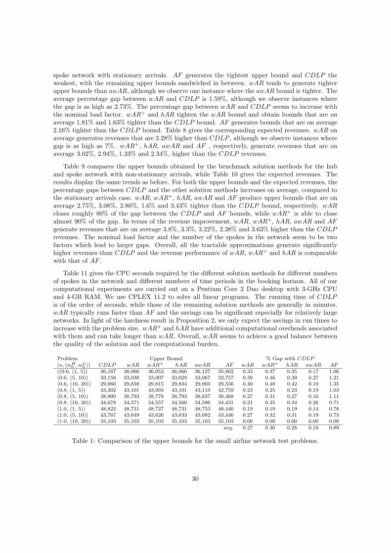
spoke network with stationary arrivals. AF generates the tightest upper bound and CDLP theweakest, with the remaining upper bounds sandwiched in between. wAR tends to generate tighterupper bounds than awAR, although we observe one instance where the awAR bound is tighter. Theaverage percentage gap between wAR and CDLP is 1.59%, although we observe instances wherethe gap is as high as 2.73%. The percentage gap between wAR and CDLP seems to increase withthe nominal load factor. wAR+ and hAR tighten the wAR bound and obtain bounds that are onaverage 1.81% and 1.63% tighter than the CDLP bound. AF generates bounds that are on average2.16% tighter than the CDLP bound. Table 8 gives the corresponding expected revenues. wAR onaverage generates revenues that are 2.28% higher than CDLP , although we observe instances wheregap is as high as 7%. wAR+, hAR, awAR and AF , respectively, generate revenues that are onaverage 3.02%, 2.94%, 1.33% and 2.34%, higher than the CDLP revenues.
Table 9 compares the upper bounds obtained by the benchmark solution methods for the huband spoke network with non-stationary arrivals, while Table 10 gives the expected revenues. Theresults display the same trends as before. For both the upper bounds and the expected revenues, thepercentage gaps between CDLP and the other solution methods increases on average, compared tothe stationary arrivals case. wAR, wAR+, hAR, awAR and AF produce upper bounds that are onaverage 2.75%, 3.08%, 2.80%, 1.6% and 3.43% tighter than the CDLP bound, respectively. wARcloses roughly 80% of the gap between the CDLP and AF bounds, while wAR+ is able to closealmost 90% of the gap. In terms of the revenue improvement, wAR, wAR+, hAR, awAR and AFgenerate revenues that are on average 3.8%, 3.3%, 3.22%, 2.38% and 3.63% higher than the CDLPrevenues. The nominal load factor and the number of the spokes in the network seem to be twofactors which lead to larger gaps. Overall, all the tractable approximations generate significantlyhigher revenues than CDLP and the revenue performance of wAR, wAR+ and hAR is comparablewith that of AF .
Table 11 gives the CPU seconds required by the different solution methods for different numbersof spokes in the network and different numbers of time periods in the booking horizon. All of ourcomputational experiments are carried out on a Pentium Core 2 Duo desktop with 3-GHz CPUand 4-GB RAM. We use CPLEX 11.2 to solve all linear programs. The running time of CDLPis of the order of seconds, while those of the remaining solution methods are generally in minutes.wAR typically runs faster than AF and the savings can be significant especially for relatively largenetworks. In light of the hardness result in Proposition 2, we only expect the savings in run times toincrease with the problem size. wAR+ and hAR have additional computational overheads associatedwith them and can take longer than wAR. Overall, wAR seems to achieve a good balance betweenthe quality of the solution and the computational burden.
Problem Upper Bound % Gap with CDLP(κ, (wH
0 , wL0 )) CDLP wAR wAR+ hAR awAR AF wAR wAR+ hAR awAR AF
((0.6, (1, 5)) 36,187 36,066 36,053 36,060 36,127 35,802 0.33 0.37 0.35 0.17 1.06(0.6, (5, 10)) 33,158 33,030 33,007 33,029 33,067 32,757 0.39 0.46 0.39 0.27 1.21(0.6, (10, 20)) 29,960 29,838 29,815 29,834 29,903 29,556 0.40 0.48 0.42 0.19 1.35(0.8, (1, 5)) 43,202 43,101 43,093 43,101 43,119 42,759 0.23 0.25 0.23 0.19 1.03(0.8, (5, 10)) 38,900 38,793 38,778 38,793 38,837 38,468 0.27 0.31 0.27 0.16 1.11(0.8, (10, 20)) 34,678 34,571 34,557 34,560 34,586 34,431 0.31 0.35 0.34 0.26 0.71(1.0, (1, 5)) 48,822 48,731 48,727 48,731 48,753 48,440 0.19 0.19 0.19 0.14 0.78(1.0, (5, 10)) 43,767 43,649 43,626 43,633 43,682 43,446 0.27 0.32 0.31 0.19 0.73(1.0, (10, 20)) 35,103 35,103 35,103 35,103 35,103 35,103 0.00 0.00 0.00 0.00 0.00
avg. 0.27 0.30 0.28 0.18 0.89
Table 1: Comparison of the upper bounds for the small airline network test problems.
30
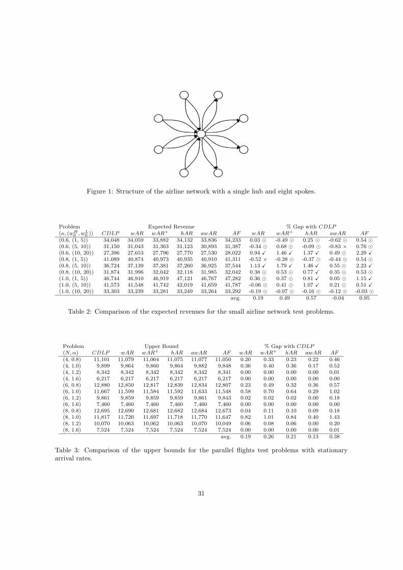
Figure 1: Structure of the airline network with a single hub and eight spokes.
Problem Expected Revenue % Gap with CDLP(κ, (wH
0 , wL0 )) CDLP wAR wAR+ hAR awAR AF wAR wAR+ hAR awAR AF
(0.6, (1, 5)) 34,048 34,059 33,882 34,132 33,836 34,233 0.03 ⊙ -0.49 ⊙ 0.25 ⊙ -0.62 ⊙ 0.54 ⊙(0.6, (5, 10)) 31,150 31,043 31,363 31,123 30,893 31,387 -0.34 ⊙ 0.68 ⊙ -0.09 ⊙ -0.83 × 0.76 ⊙(0.6, (10, 20)) 27,396 27,653 27,796 27,770 27,530 28,022 0.94 X 1.46 X 1.37 X 0.49 ⊙ 2.29 X(0.8, (1, 5)) 41,089 40,874 40,973 40,935 40,910 41,311 -0.52 × -0.28 ⊙ -0.37 ⊙ -0.44 ⊙ 0.54 ⊙(0.8, (5, 10)) 36,724 37,139 37,381 37,260 36,925 37,544 1.13 X 1.79 X 1.46 X 0.55 ⊙ 2.23 X(0.8, (10, 20)) 31,874 31,996 32,042 32,118 31,985 32,042 0.38 ⊙ 0.53 ⊙ 0.77 X 0.35 ⊙ 0.53 ⊙(1.0, (1, 5)) 46,744 46,910 46,919 47,121 46,767 47,282 0.36 ⊙ 0.37 ⊙ 0.81 X 0.05 ⊙ 1.15 X(1.0, (5, 10)) 41,573 41,548 41,742 42,019 41,659 41,787 -0.06 ⊙ 0.41 ⊙ 1.07 X 0.21 ⊙ 0.51 X(1.0, (10, 20)) 33,303 33,239 33,281 33,249 33,264 33,292 -0.19 ⊙ -0.07 ⊙ -0.16 ⊙ -0.12 ⊙ -0.03 ⊙
avg. 0.19 0.49 0.57 -0.04 0.95
Table 2: Comparison of the expected revenues for the small airline network test problems.
Problem Upper Bound % Gap with CDLP(N,α) CDLP wAR wAR+ hAR awAR AF wAR wAR+ hAR awAR AF(4, 0.8) 11,101 11,079 11,064 11,075 11,077 11,050 0.20 0.33 0.23 0.22 0.46(4, 1.0) 9,899 9,864 9,860 9,864 9,882 9,848 0.36 0.40 0.36 0.17 0.52(4, 1.2) 8,342 8,342 8,342 8,342 8,342 8,341 0.00 0.00 0.00 0.00 0.01(4, 1.6) 6,217 6,217 6,217 6,217 6,217 6,217 0.00 0.00 0.00 0.00 0.00(6, 0.8) 12,880 12,850 12,817 12,839 12,834 12,807 0.23 0.49 0.32 0.36 0.57(6, 1.0) 11,667 11,599 11,584 11,592 11,633 11,548 0.58 0.70 0.64 0.29 1.02(6, 1.2) 9,861 9,859 9,859 9,859 9,861 9,843 0.02 0.02 0.02 0.00 0.18(6, 1.6) 7,460 7,460 7,460 7,460 7,460 7,460 0.00 0.00 0.00 0.00 0.00(8, 0.8) 12,695 12,690 12,681 12,682 12,684 12,673 0.04 0.11 0.10 0.09 0.18(8, 1.0) 11,817 11,720 11,697 11,718 11,770 11,647 0.82 1.01 0.84 0.40 1.43(8, 1.2) 10,070 10,063 10,062 10,063 10,070 10,049 0.06 0.08 0.06 0.00 0.20(8, 1.6) 7,524 7,524 7,524 7,524 7,524 7,524 0.00 0.00 0.00 0.00 0.01
avg. 0.19 0.26 0.21 0.13 0.38
Table 3: Comparison of the upper bounds for the parallel flights test problems with stationaryarrival rates.
31
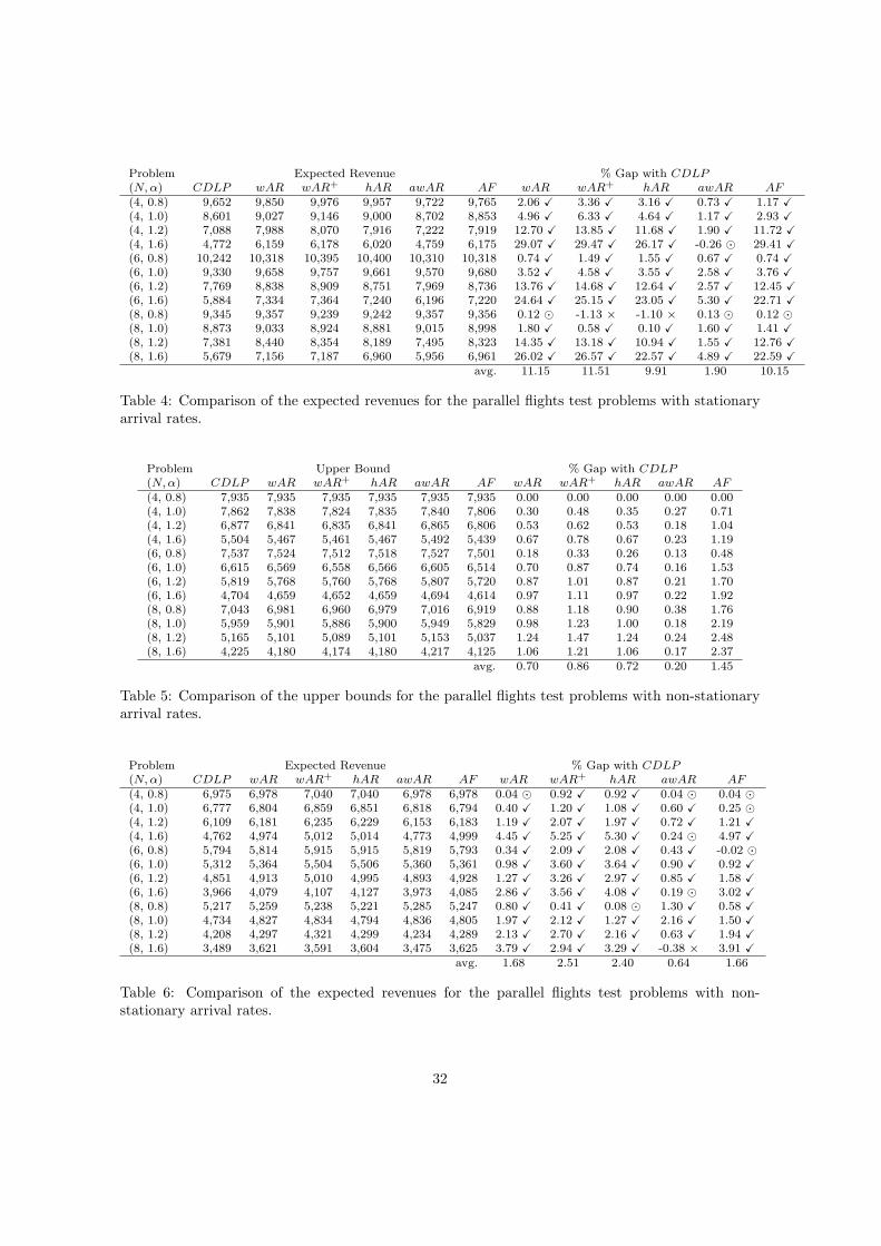
Problem Expected Revenue % Gap with CDLP(N,α) CDLP wAR wAR+ hAR awAR AF wAR wAR+ hAR awAR AF(4, 0.8) 9,652 9,850 9,976 9,957 9,722 9,765 2.06 X 3.36 X 3.16 X 0.73 X 1.17 X(4, 1.0) 8,601 9,027 9,146 9,000 8,702 8,853 4.96 X 6.33 X 4.64 X 1.17 X 2.93 X(4, 1.2) 7,088 7,988 8,070 7,916 7,222 7,919 12.70 X 13.85 X 11.68 X 1.90 X 11.72 X(4, 1.6) 4,772 6,159 6,178 6,020 4,759 6,175 29.07 X 29.47 X 26.17 X -0.26 ⊙ 29.41 X(6, 0.8) 10,242 10,318 10,395 10,400 10,310 10,318 0.74 X 1.49 X 1.55 X 0.67 X 0.74 X(6, 1.0) 9,330 9,658 9,757 9,661 9,570 9,680 3.52 X 4.58 X 3.55 X 2.58 X 3.76 X(6, 1.2) 7,769 8,838 8,909 8,751 7,969 8,736 13.76 X 14.68 X 12.64 X 2.57 X 12.45 X(6, 1.6) 5,884 7,334 7,364 7,240 6,196 7,220 24.64 X 25.15 X 23.05 X 5.30 X 22.71 X(8, 0.8) 9,345 9,357 9,239 9,242 9,357 9,356 0.12 ⊙ -1.13 × -1.10 × 0.13 ⊙ 0.12 ⊙(8, 1.0) 8,873 9,033 8,924 8,881 9,015 8,998 1.80 X 0.58 X 0.10 X 1.60 X 1.41 X(8, 1.2) 7,381 8,440 8,354 8,189 7,495 8,323 14.35 X 13.18 X 10.94 X 1.55 X 12.76 X(8, 1.6) 5,679 7,156 7,187 6,960 5,956 6,961 26.02 X 26.57 X 22.57 X 4.89 X 22.59 X
avg. 11.15 11.51 9.91 1.90 10.15
Table 4: Comparison of the expected revenues for the parallel flights test problems with stationaryarrival rates.
Problem Upper Bound % Gap with CDLP(N,α) CDLP wAR wAR+ hAR awAR AF wAR wAR+ hAR awAR AF(4, 0.8) 7,935 7,935 7,935 7,935 7,935 7,935 0.00 0.00 0.00 0.00 0.00(4, 1.0) 7,862 7,838 7,824 7,835 7,840 7,806 0.30 0.48 0.35 0.27 0.71(4, 1.2) 6,877 6,841 6,835 6,841 6,865 6,806 0.53 0.62 0.53 0.18 1.04(4, 1.6) 5,504 5,467 5,461 5,467 5,492 5,439 0.67 0.78 0.67 0.23 1.19(6, 0.8) 7,537 7,524 7,512 7,518 7,527 7,501 0.18 0.33 0.26 0.13 0.48(6, 1.0) 6,615 6,569 6,558 6,566 6,605 6,514 0.70 0.87 0.74 0.16 1.53(6, 1.2) 5,819 5,768 5,760 5,768 5,807 5,720 0.87 1.01 0.87 0.21 1.70(6, 1.6) 4,704 4,659 4,652 4,659 4,694 4,614 0.97 1.11 0.97 0.22 1.92(8, 0.8) 7,043 6,981 6,960 6,979 7,016 6,919 0.88 1.18 0.90 0.38 1.76(8, 1.0) 5,959 5,901 5,886 5,900 5,949 5,829 0.98 1.23 1.00 0.18 2.19(8, 1.2) 5,165 5,101 5,089 5,101 5,153 5,037 1.24 1.47 1.24 0.24 2.48(8, 1.6) 4,225 4,180 4,174 4,180 4,217 4,125 1.06 1.21 1.06 0.17 2.37
avg. 0.70 0.86 0.72 0.20 1.45
Table 5: Comparison of the upper bounds for the parallel flights test problems with non-stationaryarrival rates.
Problem Expected Revenue % Gap with CDLP(N,α) CDLP wAR wAR+ hAR awAR AF wAR wAR+ hAR awAR AF(4, 0.8) 6,975 6,978 7,040 7,040 6,978 6,978 0.04 ⊙ 0.92 X 0.92 X 0.04 ⊙ 0.04 ⊙(4, 1.0) 6,777 6,804 6,859 6,851 6,818 6,794 0.40 X 1.20 X 1.08 X 0.60 X 0.25 ⊙(4, 1.2) 6,109 6,181 6,235 6,229 6,153 6,183 1.19 X 2.07 X 1.97 X 0.72 X 1.21 X(4, 1.6) 4,762 4,974 5,012 5,014 4,773 4,999 4.45 X 5.25 X 5.30 X 0.24 ⊙ 4.97 X(6, 0.8) 5,794 5,814 5,915 5,915 5,819 5,793 0.34 X 2.09 X 2.08 X 0.43 X -0.02 ⊙(6, 1.0) 5,312 5,364 5,504 5,506 5,360 5,361 0.98 X 3.60 X 3.64 X 0.90 X 0.92 X(6, 1.2) 4,851 4,913 5,010 4,995 4,893 4,928 1.27 X 3.26 X 2.97 X 0.85 X 1.58 X(6, 1.6) 3,966 4,079 4,107 4,127 3,973 4,085 2.86 X 3.56 X 4.08 X 0.19 ⊙ 3.02 X(8, 0.8) 5,217 5,259 5,238 5,221 5,285 5,247 0.80 X 0.41 X 0.08 ⊙ 1.30 X 0.58 X(8, 1.0) 4,734 4,827 4,834 4,794 4,836 4,805 1.97 X 2.12 X 1.27 X 2.16 X 1.50 X(8, 1.2) 4,208 4,297 4,321 4,299 4,234 4,289 2.13 X 2.70 X 2.16 X 0.63 X 1.94 X(8, 1.6) 3,489 3,621 3,591 3,604 3,475 3,625 3.79 X 2.94 X 3.29 X -0.38 × 3.91 X
avg. 1.68 2.51 2.40 0.64 1.66
Table 6: Comparison of the expected revenues for the parallel flights test problems with non-stationary arrival rates.
32
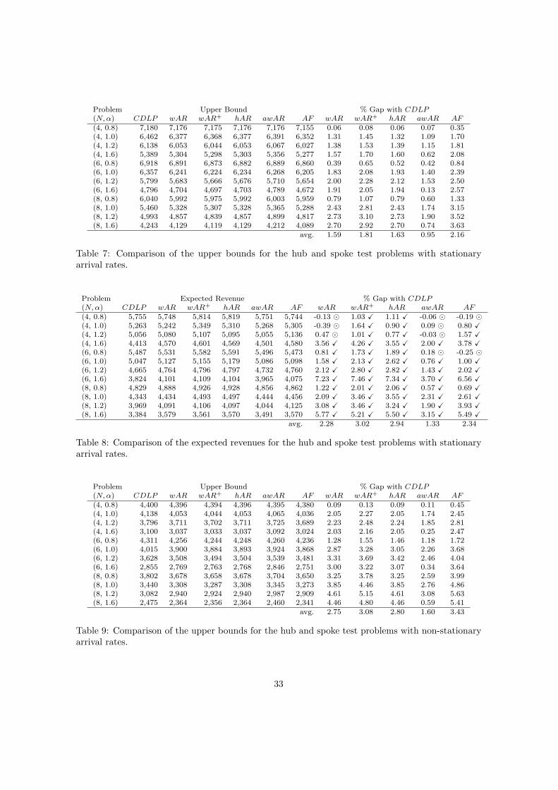
Problem Upper Bound % Gap with CDLP(N,α) CDLP wAR wAR+ hAR awAR AF wAR wAR+ hAR awAR AF(4, 0.8) 7,180 7,176 7,175 7,176 7,176 7,155 0.06 0.08 0.06 0.07 0.35(4, 1.0) 6,462 6,377 6,368 6,377 6,391 6,352 1.31 1.45 1.32 1.09 1.70(4, 1.2) 6,138 6,053 6,044 6,053 6,067 6,027 1.38 1.53 1.39 1.15 1.81(4, 1.6) 5,389 5,304 5,298 5,303 5,356 5,277 1.57 1.70 1.60 0.62 2.08(6, 0.8) 6,918 6,891 6,873 6,882 6,889 6,860 0.39 0.65 0.52 0.42 0.84(6, 1.0) 6,357 6,241 6,224 6,234 6,268 6,205 1.83 2.08 1.93 1.40 2.39(6, 1.2) 5,799 5,683 5,666 5,676 5,710 5,654 2.00 2.28 2.12 1.53 2.50(6, 1.6) 4,796 4,704 4,697 4,703 4,789 4,672 1.91 2.05 1.94 0.13 2.57(8, 0.8) 6,040 5,992 5,975 5,992 6,003 5,959 0.79 1.07 0.79 0.60 1.33(8, 1.0) 5,460 5,328 5,307 5,328 5,365 5,288 2.43 2.81 2.43 1.74 3.15(8, 1.2) 4,993 4,857 4,839 4,857 4,899 4,817 2.73 3.10 2.73 1.90 3.52(8, 1.6) 4,243 4,129 4,119 4,129 4,212 4,089 2.70 2.92 2.70 0.74 3.63
avg. 1.59 1.81 1.63 0.95 2.16
Table 7: Comparison of the upper bounds for the hub and spoke test problems with stationaryarrival rates.
Problem Expected Revenue % Gap with CDLP(N,α) CDLP wAR wAR+ hAR awAR AF wAR wAR+ hAR awAR AF(4, 0.8) 5,755 5,748 5,814 5,819 5,751 5,744 -0.13 ⊙ 1.03 X 1.11 X -0.06 ⊙ -0.19 ⊙(4, 1.0) 5,263 5,242 5,349 5,310 5,268 5,305 -0.39 ⊙ 1.64 X 0.90 X 0.09 ⊙ 0.80 X(4, 1.2) 5,056 5,080 5,107 5,095 5,055 5,136 0.47 ⊙ 1.01 X 0.77 X -0.03 ⊙ 1.57 X(4, 1.6) 4,413 4,570 4,601 4,569 4,501 4,580 3.56 X 4.26 X 3.55 X 2.00 X 3.78 X(6, 0.8) 5,487 5,531 5,582 5,591 5,496 5,473 0.81 X 1.73 X 1.89 X 0.18 ⊙ -0.25 ⊙(6, 1.0) 5,047 5,127 5,155 5,179 5,086 5,098 1.58 X 2.13 X 2.62 X 0.76 X 1.00 X(6, 1.2) 4,665 4,764 4,796 4,797 4,732 4,760 2.12 X 2.80 X 2.82 X 1.43 X 2.02 X(6, 1.6) 3,824 4,101 4,109 4,104 3,965 4,075 7.23 X 7.46 X 7.34 X 3.70 X 6.56 X(8, 0.8) 4,829 4,888 4,926 4,928 4,856 4,862 1.22 X 2.01 X 2.06 X 0.57 X 0.69 X(8, 1.0) 4,343 4,434 4,493 4,497 4,444 4,456 2.09 X 3.46 X 3.55 X 2.31 X 2.61 X(8, 1.2) 3,969 4,091 4,106 4,097 4,044 4,125 3.08 X 3.46 X 3.24 X 1.90 X 3.93 X(8, 1.6) 3,384 3,579 3,561 3,570 3,491 3,570 5.77 X 5.21 X 5.50 X 3.15 X 5.49 X
avg. 2.28 3.02 2.94 1.33 2.34
Table 8: Comparison of the expected revenues for the hub and spoke test problems with stationaryarrival rates.
Problem Upper Bound % Gap with CDLP(N,α) CDLP wAR wAR+ hAR awAR AF wAR wAR+ hAR awAR AF(4, 0.8) 4,400 4,396 4,394 4,396 4,395 4,380 0.09 0.13 0.09 0.11 0.45(4, 1.0) 4,138 4,053 4,044 4,053 4,065 4,036 2.05 2.27 2.05 1.74 2.45(4, 1.2) 3,796 3,711 3,702 3,711 3,725 3,689 2.23 2.48 2.24 1.85 2.81(4, 1.6) 3,100 3,037 3,033 3,037 3,092 3,024 2.03 2.16 2.05 0.25 2.47(6, 0.8) 4,311 4,256 4,244 4,248 4,260 4,236 1.28 1.55 1.46 1.18 1.72(6, 1.0) 4,015 3,900 3,884 3,893 3,924 3,868 2.87 3.28 3.05 2.26 3.68(6, 1.2) 3,628 3,508 3,494 3,504 3,539 3,481 3.31 3.69 3.42 2.46 4.04(6, 1.6) 2,855 2,769 2,763 2,768 2,846 2,751 3.00 3.22 3.07 0.34 3.64(8, 0.8) 3,802 3,678 3,658 3,678 3,704 3,650 3.25 3.78 3.25 2.59 3.99(8, 1.0) 3,440 3,308 3,287 3,308 3,345 3,273 3.85 4.46 3.85 2.76 4.86(8, 1.2) 3,082 2,940 2,924 2,940 2,987 2,909 4.61 5.15 4.61 3.08 5.63(8, 1.6) 2,475 2,364 2,356 2,364 2,460 2,341 4.46 4.80 4.46 0.59 5.41
avg. 2.75 3.08 2.80 1.60 3.43
Table 9: Comparison of the upper bounds for the hub and spoke test problems with non-stationaryarrival rates.
33
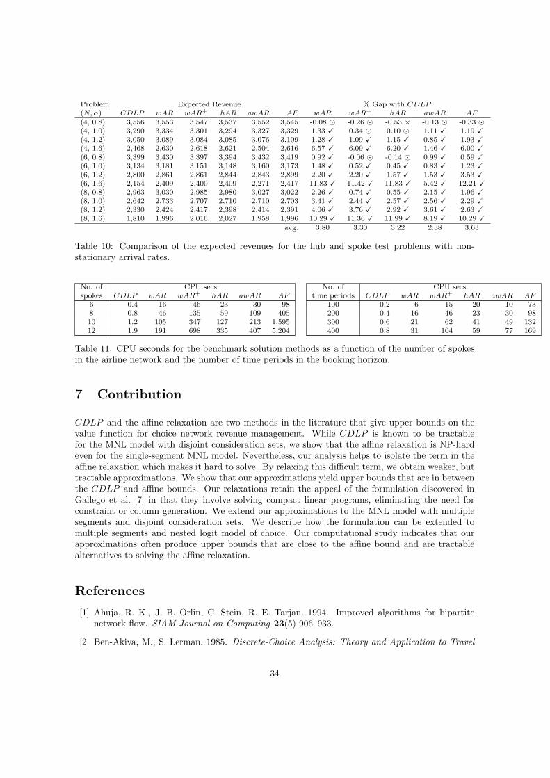
Problem Expected Revenue % Gap with CDLP(N,α) CDLP wAR wAR+ hAR awAR AF wAR wAR+ hAR awAR AF(4, 0.8) 3,556 3,553 3,547 3,537 3,552 3,545 -0.08 ⊙ -0.26 ⊙ -0.53 × -0.13 ⊙ -0.33 ⊙(4, 1.0) 3,290 3,334 3,301 3,294 3,327 3,329 1.33 X 0.34 ⊙ 0.10 ⊙ 1.11 X 1.19 X(4, 1.2) 3,050 3,089 3,084 3,085 3,076 3,109 1.28 X 1.09 X 1.15 X 0.85 X 1.93 X(4, 1.6) 2,468 2,630 2,618 2,621 2,504 2,616 6.57 X 6.09 X 6.20 X 1.46 X 6.00 X(6, 0.8) 3,399 3,430 3,397 3,394 3,432 3,419 0.92 X -0.06 ⊙ -0.14 ⊙ 0.99 X 0.59 X(6, 1.0) 3,134 3,181 3,151 3,148 3,160 3,173 1.48 X 0.52 X 0.45 X 0.83 X 1.23 X(6, 1.2) 2,800 2,861 2,861 2,844 2,843 2,899 2.20 X 2.20 X 1.57 X 1.53 X 3.53 X(6, 1.6) 2,154 2,409 2,400 2,409 2,271 2,417 11.83 X 11.42 X 11.83 X 5.42 X 12.21 X(8, 0.8) 2,963 3,030 2,985 2,980 3,027 3,022 2.26 X 0.74 X 0.55 X 2.15 X 1.96 X(8, 1.0) 2,642 2,733 2,707 2,710 2,710 2,703 3.41 X 2.44 X 2.57 X 2.56 X 2.29 X(8, 1.2) 2,330 2,424 2,417 2,398 2,414 2,391 4.06 X 3.76 X 2.92 X 3.61 X 2.63 X(8, 1.6) 1,810 1,996 2,016 2,027 1,958 1,996 10.29 X 11.36 X 11.99 X 8.19 X 10.29 X
avg. 3.80 3.30 3.22 2.38 3.63
Table 10: Comparison of the expected revenues for the hub and spoke test problems with non-stationary arrival rates.
No. of CPU secs. No. of CPU secs.spokes CDLP wAR wAR+ hAR awAR AF time periods CDLP wAR wAR+ hAR awAR AF
6 0.4 16 46 23 30 98 100 0.2 6 15 20 10 738 0.8 46 135 59 109 405 200 0.4 16 46 23 30 9810 1.2 105 347 127 213 1,595 300 0.6 21 62 41 49 13212 1.9 191 698 335 407 5,204 400 0.8 31 104 59 77 169
Table 11: CPU seconds for the benchmark solution methods as a function of the number of spokesin the airline network and the number of time periods in the booking horizon.
7 Contribution
CDLP and the affine relaxation are two methods in the literature that give upper bounds on thevalue function for choice network revenue management. While CDLP is known to be tractablefor the MNL model with disjoint consideration sets, we show that the affine relaxation is NP-hardeven for the single-segment MNL model. Nevertheless, our analysis helps to isolate the term in theaffine relaxation which makes it hard to solve. By relaxing this difficult term, we obtain weaker, buttractable approximations. We show that our approximations yield upper bounds that are in betweenthe CDLP and affine bounds. Our relaxations retain the appeal of the formulation discovered inGallego et al. [7] in that they involve solving compact linear programs, eliminating the need forconstraint or column generation. We extend our approximations to the MNL model with multiplesegments and disjoint consideration sets. We describe how the formulation can be extended tomultiple segments and nested logit model of choice. Our computational study indicates that ourapproximations often produce upper bounds that are close to the affine bound and are tractablealternatives to solving the affine relaxation.
References
[1] Ahuja, R. K., J. B. Orlin, C. Stein, R. E. Tarjan. 1994. Improved algorithms for bipartitenetwork flow. SIAM Journal on Computing 23(5) 906–933.
[2] Ben-Akiva, M., S. Lerman. 1985. Discrete-Choice Analysis: Theory and Application to Travel
34
Demand . MIT Press, Cambridge, MA.
[3] Bodea, T., M. Ferguson, L. Garrow. 2009. Choice-based revenue management: Data from amajor hotel chain. Manufacturing and Service Operations Management 11 356–361.
[4] Bront, J. J. M., I. Mendez-Dıaz, G. Vulcano. 2009. A column generation algorithm for choice-based network revenue management. Operations Research 57(3) 769–784.
[5] Davis, J. M., G. Gallego, H. Topaloglu. 2014. Assortment optimization under variants of thenested logit model. Operations Research (forthcoming) .
[6] Gallego, G., G. Iyengar, R. Phillips, A. Dubey. 2004. Managing flexible products on a network.Tech. Rep. TR-2004-01, Dept of Industrial Engineering, Columbia University, NY, NY.
[7] Gallego, G., R. Ratliff, S. Shebalov. 2010. A general attraction model and an efficient formula-tion for the network revenue management problem. Tech. rep., Department of IEOR, ColumbiaUniversity, available at http://www.columbia.edu/~gmg2/, retrieved Jan 13, 2012.
[8] Kunnumkal, S., H. Topaloglu. 2010. A new dynamic programming decomposition method forthe network revenue management problem with customer choice behavior. Production andOperations Management 19(5) 575–590.
[9] Liu, Q., G. J. van Ryzin. 2008. On the choice-based linear programming model for networkrevenue management. Manufacturing and Service Operations Management 10(2) 288–310.
[10] Meissner, J., A. K. Strauss. 2012. Network revenue management with inventory-sensitive bidprices and customer choice. European Journal of Operational Research 216(2) 459–468.
[11] Meissner, J., A. K. Strauss, K. T. Talluri. 2013. An enhanced concave programming methodfor choice network revenue management. Production and Operations Management 22(1) 71–87.
[12] Newman, J.P., M. Ferguson, L. Garrow, T. Jacobs. 2012. Estimation of choice-based modelsusing sales data from a single firm. Tech. rep., Georgia Institute of Technology.
[13] Peeters, R. 2003. The maximum edge biclique problem is NP-complete. Discrete AppliedMathematics 131 651–654.
[14] Rusmevichientong, P., D. Shmoys, C. Tong, H. Topaloglu. 2014. Assortment optimizationunder the multinomial logit model with random choice parameters. Production and OperationsManagement (forthcoming) .
[15] Strauss, A.K, K. T. Talluri. 2012. A tractable consideration set structure for network revenuemanagement. Tech. rep., Working Paper 1303, Department of Economics, Universitat PompeuFabra, available at http://www.econ.upf.edu/en/research/onepaper.php?id=1215.
[16] Talluri, K. T. 2009. A finite-population revenue management model and a risk-ratio procedurefor the joint estimation of population size and parameters. Tech. rep., Working Paper 1141,Department of Economics, Universitat Pompeu Fabra, Barcelona, Spain.
[17] Talluri, K. T. 2014. New formulations for choice network revenue management. INFORMSJournal of Computing (to appear) .
[18] Talluri, K. T., G. J. van Ryzin. 2004. Revenue management under a general discrete choicemodel of consumer behavior. Management Science 50(1) 15–33.
35
[19] Talluri, K. T., G. J. van Ryzin. 2004. The Theory and Practice of Revenue Management .Kluwer, New York, NY.
[20] Topaloglu, H. 2013. Joint stocking and product offer decisions under the multinomial logitmodel. Production and Operations Management 22 1182–1199.
[21] Vossen, T. W. M., D Zhang. 2012. A dynamic disaggregation approach to approximate linearprograms for network revenue management. Tech. rep., Leeds School of Business, University ofColorado at Boulder, Boulder, CO.
[22] Vulcano, G., G. van Ryzin, W. Chaar. 2010. A choice-based revenue management: An empiricalstudy of estimation and optimization. MSOM 12(3) 371–392.
[23] Zhang, D., D. Adelman. 2009. An approximate dynamic programming approach to networkrevenue management with customer choice. Transportation Science 43(3) 381–394.
Appendix A: A continuous relaxation of the affine separationproblem
We show that wAR gives a tighter upper bound than a continuous relaxation of the AF separationproblem. We first describe the continuous relaxation and then show that wAR gives a tighter upperbound than the continuous relaxation. We use the following result, which follows from Theorem 1 in[20]. Throughout, we assume that the choice probabilities are according to the MNL choice modeland that the no-purchase preference weight is normalized to 1.
Theorem 1. Let H = {∑S hSPj(S) | 0 ≤ hS ≤ 1,
∑S hS = 1} and let Y = {(y0, {yj | ∀j}) | y0 +∑
j yj = 1, yj/wj − y0 ≤ 0, ∀j, yj , y0 ≥ 0}. We have H = Y.
Note that in Theorem 1 above, we can interpret yj as being the sales rate of product j. We nowgive an equivalent formulation of the AF separation problem in terms of the sales rates. Recall,from constraints (11) that the AF separation problem is to check if
βt ≥ ΠRAFt (γ) = maxS
∑j
λPj(S)
fj − ∑i∈Ij
τ∑k=t+1
γi,k
−∑i
γi,t1[i∈IS ]
.
Introducing variables hS to indicate if set S is offered and qi to indicate if resource i is open, andnoting that we write i ∈ IS whenever there is a j ∈ S with i ∈ Ij , the above maximization problemcan be equivalently written as
ΠRAFt (γ) = maxh,q
∑S
hS
∑j
λPj(S)
fj − ∑i∈Ij
τ∑k=t+1
γi,k
−∑i
γi,tqi
s.t
(∑S
Pj(S)hS
)/wj ≤ qi, ∀i ∈ Ij , j (44)∑
S
hS = 1
hS ∈ {0, 1}, qi ∈ {0, 1}.
36
We note that since Pj(S) > 0 for j ∈ S and Pj(S) = 0 for j /∈ S, constraints (44) ensure thatqi = 1 for all i ∈ IS with hS = 1. Now observe that we can replace the integrality constraint onhS with 0 ≤ hS ≤ 1 without affecting the optimal objective function value. After doing this and byappealing to Theorem 1, we can obtain ΠRAFt (γ), through the following equivalent, sales-rate based,formulation:
ΠRAFt (γ) = maxy,q
∑j
λ
fj − ∑i∈Ij
τ∑k=t+1
γi,k
yj −∑i
γi,tqi (45)
s.t yj/wj ≤ qi, ∀i ∈ Ij , j (46)
y0 +∑j
yj = 1 (47)
yj/wj − y0 ≤ 0 ∀j (48)
yj , y0 ≥ 0, qi ∈ {0, 1}. (49)
The above, sales-rate based formulation motivates our continuous relaxation of the AF separationproblem, where we relax the integrality requirement on qi by replacing it with the constraint 0 ≤qi ≤ 1 and solve an LP. In other words, if we let ΠAFCR
t (γ) denote the optimal objective functionvalue of the continuous relaxation of (45)–(49), we replace the AF constraint βt ≥ ΠRAFt (γ) withβt ≥ ΠAFCR
t (γ). It is clear that by separating over the continuous relaxation, we get an upper boundthat is weaker than AF . We show below that the resulting upper bound is weaker than the wARbound as well. We first take the dual of the continuous relaxation of (45)–(49), which after somesimplifications is
ΠAFCRt (γ) = min
π,z
∑i
∑j∈Ji
πi,j − γi,t
+∑j
zj
s.t∑i∈Ij
πi,j/wj +∑j′
zj′ + zj/wj ≥ λ
fj − ∑i∈Ij
τ∑k=t+1
γi,k
∀j
∑j∈Ji
πi,j − γi,t ≥ 0 ∀i
πi,j , zj ≥ 0.
Folding the dual back into RAF by following the same steps as in §4.3, we obtain the following LP:
V AFCR = minβ,γ,π,z
∑t
βt +∑t
∑i
γi,tr1i
s.t βt −∑i
∑j∈Ji
πi,j,t +∑i
γi,t −∑j
zj,t ≥ 0 ∀t
(AFCR)∑i∈Ij
πi,j,t/wj +∑j′
zj′,t + zj,t/wj + λτ∑
k=t+1
∑i∈Ij
γi,k ≥ λfj ∀j, t
∑j∈Ji
πi,j,t − γi,t ≥ 0 ∀i, t
γi,t, zj,t, πi,j,t ≥ 0.
37
Taking the dual of AFCR and after some simplifications we get
V dAFCR = maxx,ρ
∑t
∑j
λfjxj,t
s.t x0,t + λ
t−1∑s=1
∑j∈Ji
xj,s +∑j
xj,t − ρi,t ≤ r1i ∀i, t
(dAFCR) x0,t +∑j
xj,t = 1 ∀t
xj,twj
− 1 + ρi,t ≤ 0, ∀i, j ∈ Ji, t
xj,twj
− x0,t ≤ 0 ∀j, t
x0,t, xj,t, ρi,t ≥ 0.
We have the following lemma.
Lemma 4. V wAR ≤ V AFCR
ProofNote that the second constraint in dAFCR implies that x0,t ≤ 1. Therefore,
xj,t
wj− x0,t + ρi,t ≥
xj,t
wj− 1+ ρi,t. Since ρi,t ≥ 0, we also have
xj,t
wj− x0,t + ρi,t ≥ xj,t
wj− x0,t. Comparing the constraints
of dAFCR with those of dwAR, we see that any feasible solution to dwAR is also feasible to dAFCR.The result follows by noting that dAFCR and dwAR have the same objective function.
2
Appendix B: Alternative weak affine relaxation
In this section we describe a complementary, tractable relaxation that uses a different bound thanweak affine relaxation. We refer to this method as alternative weak affine relaxation (awAR). Weshow that it also gives an upper bound on the value function and that this bound is weaker thanthe AF bound. We describe awAR for the single-segment MNL model, but all of the developmentgoes through when there are multiple segments by following the steps in §5.
awAR is based on the following identity:
Proposition 6. γS,t
(∑j∈S wj
)≥∑i,j
[1[i∈IS ] + 1[j∈S] − 1
]γi,twj+
∑i
[1− 1[i∈IS ]
] (∑j∈Ji
γi,twj
).
ProofThe right hand side can be written as
γS,t
∑j∈S
wj
−∑
{i,j |1[i∈IS ]=0,1[j∈S]=0}
γi,twj +∑i
[1− 1[i∈IS ]
]∑j∈Ji
γi,twj
.
38
So it is enough to show that
−∑
{i,j |1[i∈IS ]=0,1[j∈S]=0}
γi,twj +∑i
[1− 1[i∈IS ]
]∑j∈Ji
γi,twj
≤ 0.
Examining the term,
−∑
{i,j |1[i∈IS ]=0,1[j∈S]=0}
γi,twj +∑i
[1− 1[i∈IS ]
]∑j∈Ji
γi,twj
= −
∑{i,j |1[i∈IS ]=0,1[j∈S]=0}
γi,twj +∑i ∈IS
γi,t
∑j∈Ji
wj
= −
∑{i,j | i ∈IS ,j ∈S}
γi,twj +∑i ∈IS
γi,t
∑j∈Ji
wj
= −
∑{i,j | i ∈IS ,j ∈S,i ∈Ij}
γi,twj −∑i∈IS
γi,t
∑j∈Ji
wj
+∑i ∈IS
γi,t
∑j∈Ji
wj
≤ 0,
where the last equality follows from the fact that for all i ∈ {i | i ∈ IS} we cannot have a j ∈ S withi ∈ Ij .
2
Proposition 6 implies that ΠAFt (β, γ) ≤ ΠawARt (β, γ) where
ΠawARt (β, γ) = maxS
−γS,t −∑i,j
[1[i∈IS ] + 1[j∈S] − 1
]γi,twj −
∑i
[1− 1[i∈IS ]
]∑j∈Ji
γi,twj
−∑j∈S
wj
βt + λ
i∑∈Ij
∑k=t+1
γi,k
− fj
. (50)
We replace the right hand side of constraint (16) with ΠawARt (β, γ) and solve the LP
V awAR = minβ,γ
∑t
βt +∑t
∑i
γi,tr1i
(awAR) s.t. βt ≥ ΠawARt (β, γ) ∀tγi,t ≥ 0.
Lemma 1 now implies that V AF ≤ V awAR.
Finally, we note that the awAR bound can be computed in a tractable manner since the sep-aration problem (50) can be solved as the following integer program with a totally-unimodular
39
constraint matrix:
ΠawARt (β, γ) = maxq,u
−∑j
wj
βt + λ
∑i∈Ij
τ∑k=t+1
γi,k
− fj
uj −∑i,j
[uj + qi − 1] γi,twj
−∑i
[1− qi] γi,t
∑j∈Ji
wj
−∑i
γi,tqi
s.t. (22)− (24).
This can be folded into the original problem to obtain a compact formulation the same way as in§4.3; we omit the details.
40