Journal of Sound and Vibration (1998) 215(3), 547–569Article No. sv981709

LINEAR DAMPING MODELS FOR STRUCTURALVIBRATION

J. W

Department of Engineering, University of Cambridge, Trumpington Street,Cambridge CB2 1PZ, England

(Received 12 January 1998, and in final form 24 April 1998)

Linear damping models for structural vibration are examined: first the familiardissipation-matrix model, then the general linear model. In both cases, an approximationof small damping is used to obtain simple expressions for damped natural frequencies,complex mode shapes, and transfer functions. Results for transfer functions can beexpressed in the form of very direct extensions of the familiar expression for the undampedcase. This allows a detailed discussion of the implications of the various damping modelsfor the interpretation of measured transfer functions, especially in the context ofexperimental modal analysis. In the case of a dissipation-matrix model, it would be possiblein principle to determine all the model parameters from measurements. In the case of thegeneral model, however, there is a fundamental ambiguity which prevents fulldetermination of the model from measurements on a single structure.

7 1998 Academic Press

1. INTRODUCTION

All structures exhibit vibration damping, but despite a large literature on the subjectdamping remains one of the least well-understood aspects of general vibration analysis.The major reason for this is the absence of a universal mathematical model to representdamping forces. There are excellent reasons why the stiffness and inertia properties of ageneral discrete system, executing small vibrations around a position of stable equilibrium,may be approximated via the familiar stiffness and mass matrices. These simply representthe first non-trivial terms which do not vanish when the potential and kinetic energyfunctions are Taylor-expanded for small amplitudes of motion [1]. Nothing so simple canbe done to represent damping, because it is not in general clear which state variables thedamping forces will depend on. A commonly-used model, originated by Rayleigh [1],supposes that instantaneous generalized velocities are the only relevant state variables.Taylor expansion then leads to a model which encapsulates damping behaviour in adissipation matrix, directly analogous to the mass and stiffness matrices. This model willbe examined in some detail in this paper.

However, it is important to avoid the widespread misconception that this is the onlylinear model of vibration damping. It is perfectly possible for damping forces to dependon values of other quantities, or equivalently to depend, via convolution integrals, on thepast history of the motion. Any such model which guarantees that the energy dissipationrate is non-negative can be a potential candidate to represent the damping of a givenstructure. The dissipation-matrix model is just one among many such models.

The appropriate choice of model depends, of course, on the detailed mechanism(s) ofdamping. Unfortunately, these mechanisms are more varied and less well-understood thanthe physical mechanisms governing stiffness and inertia. A very brief review is useful to

0022–460X/98/330547+23 $30.00/0 7 1998 Academic Press

. 548

set the scene. In broad terms, structural damping mechanisms can be divided into threeclasses: (1) energy dissipation distributed throughout the bulk material making up thestructure, which can generically be called ‘‘material damping’’; (2) dissipation associatedwith junctions or interfaces between parts of the structure, generically ‘‘boundarydamping’’; and (3) dissipation associated with a fluid in contact with the structure,involving either local viscous effects or radiation away into the fluid.

Material damping can arise from a variety of microstructural mechanisms (see e.g.,reference [2]) but for small strains it is often adequate to represent it through an equivalentlinear, viscoelastic continuum model of the material. Damping can then be taken intoaccount via the ‘‘viscoelastic correspondence principle’’, which leads to the conceptof complex moduli [3]. For sinusoidal motion at a given frequency v, the effects ofviscoelasticity can be exactly represented by replacing each of the real elastic constantsof the material by a suitable complex value. The number of independent elastic constantsfor a given material is governed by its microscopic symmetries as usual—an isotropicmaterial requires two, a general orthotropic material requires nine and so on.

It is important to keep in mind that complex moduli must be defined in the frequencydomain. Although it is often found empirically that complex moduli are almostindependent of frequency in the low audio range, considerations of causality [4] show thatit is not possible for the complex moduli to be entirely independent of frequency. If inverseFourier transformation is used to obtain results in the time domain, this inevitablefrequency dependence of the complex moduli must be taken into account. Failure to dothis properly leads to the notion of ‘‘a differential equation with frequency-dependentcoefficients’’, which is all too often encountered in the literature. As has been pointed outforcibly by Crandall [4], this is a mathematical nonsense because it mixes time-domain andfrequency-domain concepts, and is likely to lead to fallacious results. In particular, itdisguises the distinction between linear and non-linear models: the cases with constantcoefficients and frequency-dependent coefficients are often described as ‘‘linear’’ and‘‘non-linear’’, respectively, when in reality both are linear models.

‘‘Boundary damping’’ is less easy to model than material damping, but it is of crucialimportance in most engineering structures. When damping is measured on a built-upstructure like a ship or a building, it is commonly found to be at least an order ofmagnitude higher than the intrinsic material damping of the main components of thestructure. This difference is attributed to effects such as frictional micro-slipping at jointsand air-pumping in riveted seams, but this attribution is usually based on negative evidence(‘‘what else could it be?’’) rather than on any attempt at detailed modelling. A familiarexample would be a window pane in a substantial masonry wall. The intrinsic dampingof glass is extremely low, but the damping of an in-situ window is far higher. Theimpedance mismatch to the wall is very high, so the energy is presumably being lostprimarily in boundary effects associated with the putty joint holding the glass to the frame,or perhaps the bolts and cement holding the frame to the wall.

In such a system the energy loss mechanism would no doubt be significantly non-linearif examined in detail, and if there is a justification for approximating the behaviour by alinear theory it probably depends on an assumption of ‘‘small damping’’. This issue hasbeen discussed by Heckl [5, 6], who found that linear theory produced acceptable responsepredictions for panels whose main damping mechanism arose from a bolted-on beam. (Heattributed the damping mechanism primarily to air-pumping between beam and panel.)

Is the ‘‘dissipation matrix’’ model of damping suitable for describing any of these effects?For some systems it is certainly appropriate—examples might be vehicle suspensions with‘‘shock absorbers’’ which are approximately classical dashpots, and other systems in whichfluid viscosity is the main energy dissipation mechanism. However, for most physical

549

mechanisms of material or boundary damping it is far from obvious that instantaneousgeneralized velocities will be the only state variables determining the rate of energydissipation, even to a first approximation. In this paper the dissipation-matrix model isconsidered, and then the results are compared with those from the most general linearmodel of damping. In both cases, a small-damping approximation is used to obtain simpleexpressions for complex frequencies and mode shapes, and for transfer functions.

Within the scope of this approximation, it is possible to address some general questions.Given a particular physical system, how could one determine experimentally whether aparticular damping model (such as a dissipation-matrix model) is appropriate? If aparticular model can be fitted to a set of measurements to satisfactory accuracy, does thatmean that the underlying physical mechanisms have been well represented? Will the effectof structural modifications be well predicted? Could an entirely different damping modelbe fitted equally well to the same set of measurements? Would that matter for the accuracyof prediction of system behaviour, or of the efficacy of vibration-control measures?

A question of particular interest concerns the ‘‘complex mode shapes’’ often revealedby experimental modal analysis [7]. Within the small-damping approximation, it will turnout to be rather easy to examine the significance of such complex shapes. It will be shownthat the pole-fitting approach to experimental modal analysis can indeed be used todiscover the correct complex modes, even for the most general linear model of dampingforces. Modal analysis might thus be able to give an experimental procedure fordetermining the parameter values of a given damping model, and of testing the validityof different damping models. However, care must be exercised because it is not a prioriobvious that reciprocity between excitation and observing points will necessarily hold ingeneral.

2. SMALL DAMPING IN THE DISSIPATION-MATRIX MODEL

2.1.

A discrete system with N degrees of freedom, executing small vibrations about a positionof stable equilibrium and with damping governed by a dissipation matrix, obeys thegoverning equations

My+Cy+Ky= f, (1)

where M, C and K are the mass, dissipation and stiffness matrices respectively, y is thevector of generalized co-ordinates, and f is the vector of generalized forces driving thevibration. By analogy with the kinetic and potential energy functions, Rayleigh’sdissipation function is defined by

F= 12ytCy, (2)

and is equal to half the rate of energy dissipation. The dissipation matrix is symmetric andpositive semi-definite.

Treatments in the literature of the coupled equations (1) usually follow one of tworoutes. Either it is assumed that C is simultaneously diagonalizable with M and K, so-calledproportional damping, or else the equations are recast into the form of 2N coupledfirst-order equations (e.g., reference [8]), which allows solutions to be computed readilybut which loses much of the intuitive immediacy of the familiar treatment of the undampedcase via normal modes. Instead, a route pioneered by Rayleigh himself is followed here,and approximate solutions of equation (1) are considered which assume that the terms ofthe dissipation matrix are small but not otherwise constrained. The motivation for this lies

. 550

in application to engineering systems which one would consider studying by experimentalmodal analysis—in such systems damping is invariably small, typically of the order of 1%of critical damping.

Consider first the undamped natural frequencies vn and corresponding mode shapevectors u(n): these satisfy

Ku(n) =v2n Mu(n), n=1, . . . , N, (3)

and the vectors may be normalized as usual by requiring

u(n)tMu(n) = 1, n=1, . . . , N. (4)

Now for free motion (i.e., f=0) of the damped system, the complex frequencies will bethe roots of

det [−v2M+ivC+K]=0. (5)

For small damping, one would expect to find roots of this equation close to 2vn for eachvalue of n, with corresponding displacement vectors y close to u(n). (Special cases involvingdegeneracies will be ignored throughout this paper.) Denote these complex solutions vn

and u(n). Seek a solution

u(n) = sN

j=1

aju(j) where an =1, =aj =�1 (j$ n). (6)

Substituting into equation (1), multiplying on the left by the transposed vector u(k)t andusing the orthogonality properties of the undamped modes yields

−v2ak +iv sj

C'kjaj +v2kak =0, (7)

where

C'kj = u(k)tCu(j) (8)

is the dissipation matrix expressed in normal co-ordinates. Using equation (6), the nthequation of the set (7) yields

v2n − v2

n +ivnC'nn 1 0,

so that

vn 12vn +iC'nn /2, (9)

while the kth equation (k$ n) yields

ak 12ivnC'kn

(v2n −v2

k ),

so that

u(n) 1 u(n) + i sk$ n

vnC'knu(k)

(v2n −v2

k ). (10)

These are Rayleigh’s results [1, section 102, equations (5) and (6)]. Equation (9) shows thatthe damped natural frequencies depend (to this order of approximation) only on thediagonal terms of the dissipation matrix in normal co-ordinates. Equation (10) shows that

kk

k k

c

y1 y2 y3

m m m

551

the off-diagonal terms of the transformed dissipation matrix C' govern the modified ‘‘modeshapes’’, which are now in general complex. Within this model the complex modes consistapproximately of a real part which is the undamped mode shape, and an imaginary partwhich is a mixture of the other undamped mode shapes. It follows that the imaginary partshould be orthogonal to the real part (with respect to the mass or stiffness matrices).

The extra contributions to mode shape are weighted to favour modes close in naturalfrequency to the one in question because of the term in the denominator. When k and nrefer to two adjacent modes, the weighting factor can be rewritten, approximately, using

vnC'kn

(v2n −v2

k )1 1

2mgkn

where

gkn =C'kn /C'nn ,

and m is the modal overlap factor of the two modes. Thus, significantly complex modesare to be expected whenever the modal overlap is not small and the off-diagonal dampingterms are comparable with the diagonal terms.

2.2.

One useful application of these approximations lies in the fact that the dampedfrequencies and mode shapes can be deduced readily from the undamped ones. Thus anelastic solution, whether analytic or based on, for example, finite-element computation, canbe readily augmented to a damped solution without the necessity to assume proportionaldamping or to solve a more complicated problem (e.g., using the first-order formulation).It is rather rare in a structural vibration problem to need more accuracy than theseequations yield: in practice the damping model is likely to be uncertain, and normally oneneither expects nor requires estimates of damping to be more accurate than, perhaps,220%.

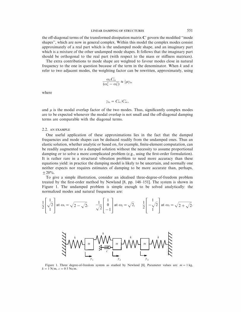
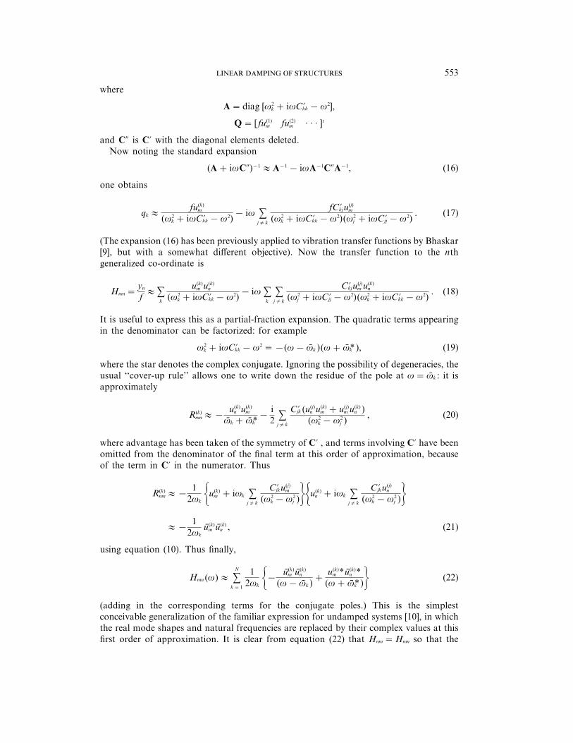
To give a simple illustration, consider an idealised three-degree-of-freedom problemtreated by the first-order method by Newland [8, pp. 148–151]. The system is shown inFigure 1. The undamped problem is simple enough to be solved analytically: thenormalized modes and natural frequencies are:

12 & 1

z21 ' at v1 =z2−z2,

1z2 & 1

0−1' at v2 =z2,

12 & 1

−z21 ' at v3 =z2+z2.

Figure 1. Three degree-of-freedom system as studied by Newland [8]. Parameter values are: m=1 kg,k=1 N/m, c=0·3 Ns/m.

. 552

The dissipation matrix is

C= &000 00·30

000',

so that

C'= & 1/21/z21/2

1/z20

−1/z2

1/2−1/z2

1/2 '&000 00·30

000'& 1/2

1/z21/2

1/z20

−1/z2

1/2−1/z2

1/2 '= & 0·15

0−0·15

000

−0·150

0·15 '.Substitution into equation (9) thus gives the approximate damped frequencies as follows:

v1 1v1 +0·075i, v2 1v2, v3 1v3 +0·075i, (11)

with corresponding approximate mode shapes:

u(1) 1 & 1/21/z21/2 '+ iv1

v23 −v2

1(−0·15)& 1/2

−1/z21/2 '1 & 1/2

1/z21/2 '−i0·041& 1/2

−1/z21/2 ', (12a)

u(2) 1 u(2), (12b)

u(3) 1 & 1/2−1/z2

1/2 '+ iv3

v21 −v2

3(−0·15)& 1/2

1/z21/2 '1 & 1/2

−1/z21/2 '+i0·098& 1/2

1/z21/2 '. (12c)

These all agree with Newland’s results to excellent accuracy.

2.3.

The same small-damping approximation can be used to obtain a surprisingly simpleexpression for the matrix of transfer functions (receptances, mobilities etc.). Suppose thatthe forcing vector f is zero for all entries except the mth, which has harmonic forcing f eivt.Write the response vector

y= sj

qju(j) eivt. (13)

Substituting into equation (1) and multiplying on the left by u(k)t gives

−v2qk +iv sj

C'kjqj +v2kqk = u(k)tf= fu(k)

m (14)

or

[A+ivC0]q=Q, (15)

553

where

A=diag [v2k +ivC'kk −v2],

Q=[ fu(1)m fu(2)

m · · · ]t

and C0 is C' with the diagonal elements deleted.Now noting the standard expansion

(A+ivC0)−1 1A−1 − ivA−1C0A−1, (16)

one obtains

qk 1fu(k)

m

(v2k +ivC'kk −v2)

− iv sj$ k

fC'kju(j)m

(v2k +ivC'kk −v2)(v2

j +ivC'jj −v2). (17)

(The expansion (16) has been previously applied to vibration transfer functions by Bhaskar[9], but with a somewhat different objective). Now the transfer function to the nthgeneralized co-ordinate is

Hmn =yn

f1 s

k

u(k)m u(k)

n

(v2k +ivC'kk −v2)

− iv sk

sj$ k

C'kju(j)m u(k)

n

(v2j +ivC'jj −v2)(v2

k +ivC'kk −v2). (18)

It is useful to express this as a partial-fraction expansion. The quadratic terms appearingin the denominator can be factorized: for example

v2k +ivC'kk −v2 =−(v− vk )(v+ v*k ), (19)

where the star denotes the complex conjugate. Ignoring the possibility of degeneracies, theusual ‘‘cover-up rule’’ allows one to write down the residue of the pole at v= vk : it isapproximately

R(k)mn 1−

u(k)n u(k)

m

vk + v*k−

i2

sj$ k

C'jk (u(j)n u(k)

m + u(j)m u(k)

n )(v2

k −v2j )

, (20)

where advantage has been taken of the symmetry of C' , and terms involving C' have beenomitted from the denominator of the final term at this order of approximation, becauseof the term in C' in the numerator. Thus

R(k)mn 1−

12vk 6u(k)

m +ivk sj$ k

C'jku(j)m

(v2k −v2

j )76u(k)n +ivk s

j$ k

C'jku(j)n

(v2k −v2

j )71−

12vk

u(k)m u(k)

n , (21)

using equation (10). Thus finally,

Hmn (v)1 sN

k=1

12vk 6− u(k)

m u(k)n

(v− vk )+

u(k)m *u(k)

n *(v+ v*k )7 (22)

(adding in the corresponding terms for the conjugate poles.) This is the simplestconceivable generalization of the familiar expression for undamped systems [10], in whichthe real mode shapes and natural frequencies are replaced by their complex values at thisfirst order of approximation. It is clear from equation (22) that Hnm =Hmn so that the

. 554

principle of reciprocity between excitation and observing points (or generalizedco-ordinates) applies. Reciprocity should not be taken for granted in all linear vibrationproblems, though. It is certainly not obvious that it will hold for linear damping modelsother than the one considered so far.

For this case in which the damping is represented by a dissipation matrix, a result verysimilar to equation (22) can be proved exactly using the first-order formalism [11]. Thedetails are given in the Appendix. The term in braces turns out to be exactly correct,provided the exact complex frequencies and mode shapes are used. But the factor (1/2vk )is replaced by a more complicated expression which reduces to this value in thezero-damping limit. The reason for presenting the approximate analysis in this section isthat when one proceeds to the case of general linear damping there is no equivalent ofthe first-order method, but the approximate analysis carries over very straightforwardly.

3. GENERAL LINEAR DAMPING

3.1.

The next step is to put the dissipation-matrix model in the context of the most generallinear model of damping in a discrete system. Suppose that the main stiffness and inertiabehaviour of the system has been represented by potential and kinetic energy functions,approximated as quadratic forms for small-amplitude motion and thus described via theusual stiffness and mass matrices. Any other internal forces within the system, includingthose responsible for dissipation of energy, will now appear as generalized forces. If thegeneralized co-ordinates are qk (t), k=1, . . . , N then motion of the system correspondingto each co-ordinate will in general result in contributions to all N generalized forces Qj .For linear behaviour the individual contributions can be expressed as convolutionintegrals, and the total generalized force is simply a sum of these:

Qj (t)=− sN

k=1 gt

t=−a

gjk (t− t)qk (t) dt. (23)

The negative sign and the choice of qk rather than qk within this expression are purely forconvenience—integration by parts would give an expression involving qk instead, withkernel functions gjk (t). The particular case in which the kernel functions are all Dirac deltafunctions and their matrix of coefficients is symmetric recovers the dissipation-matrixmodel of the previous section. The kernel functions gjk (t), or others closely related to them,are described under many different names in the literatures of different subjects: examplesare ‘‘retardation functions’’, ‘‘heredity functions’’, ‘‘after-effect functions’’ and ‘‘relaxationfunctions’’. Note that any set of generalized co-ordinates may be used in this formalism,including normal co-ordinates, in which the mass and stiffness matrices have beendiagonalised.

The rate of energy dissipation is now given by

2F= sj

qjQj = sj

sk

qj gt

t=−a

gjk (t− t)qk (t) dt. (24)

Any set of kernel functions which guarantee that this function is positive semi-definite givesa model which does not obviously contradict the laws of physics. From this definition,there is no reason in general to expect the matrix gjk (t) to be symmetric. A singlecounter-example is sufficient to demonstrate this. If the kernels are all delta functions but

555

with a skew-symmetric matrix of coefficients, the resulting model describes what areusually called ‘‘gyrostatic’’ [1] or ‘‘gyroscopic’’ [12] forces. It is obvious from equation (24)that this is a conservative effect, since the dissipation rate is zero as the terms cancel inpairs. This case is not ruled out by the criterion of non-negative energy dissipation. Indeed,such gyroscopic forces arise occasionally in the modelling of physical phenomena.

This example suggests that one might separate ‘‘damping forces’’ from other internalforces by expressing the matrix of kernels as the sum of a symmetric and a skew-symmetricpart. It is easiest to formulate the argument in the frequency domain. Suppose the systemis forced in some way at frequency v, so that the kth generalized co-ordinate respondsas qk eivt. The mean rate of energy dissipation by internal forces is then

2F=12

sj

Re (q*j Qj )=v2

2Re 6sj,k q*j Gjk (v)qk7, (25)

where * denotes the complex conjugate, and Gjk (v) is the Fourier transform of gjk (t).Decompose this matrix G into the sum of Hermitian-symmetric and Hermitian-antisym-metric parts:

G=G(s) +G(a) 0 12[G+G*t]+ 1

2[G−G*t]. (26)

It is then clear that G(a) contributes nothing to the dissipation rate in equation (25), sinceeach pair of terms consists of the difference between a number and its complex conjugate.All ‘‘damping’’ forces are described by G(s), while G(a) describes what might be called‘‘generalized gyroscopic forces’’. Whether this distinction carries any physical significance,however, will depend on the detailed mechanisms of the internal forces.

3.2.

For harmonic excitation of a single generalized co-ordinate of a discrete system subjectto the generalized forces (23), the set of equations of motion equivalent to (14) is

−v2qk +iv sj

G'kjqj +v2kqk = fu(k)

m , (27)

where

G'kj = u(k)tGu(j) (28)

is expressed in normal co-ordinates, exactly analogous to equation (8). The only differencesbetween equations (27) and (14) are that G'kj may depend on frequency while C'kj did not,and that G'kj may not be symmetric. To obtain the set of transfer functions analogous toequation (18) involves inverting the matrix

D=diag [v2k −v2]+ ivG'. (29)

Before obtaining an explicit expression for the inverse using the small-dampingapproximation, it is worth noting an important deduction which is not a priori obvious.All transfer functions will have poles corresponding to the zeros of the determinant of D,and these poles are therefore guaranteed to be the same for all possible transfer functions,apart from special cases where a residue happens to be zero. There may also be additionalpoles associated with the frequency-dependence of the terms of G', but it is the former setof poles which includes the ‘‘damped resonances’’ if damping is in some sense light.

It will now be assumed that damping is light, in the sense that the terms =G'kj (v)= aresmall for frequencies within the range of interest, covering the undamped resonance

. 556

frequencies of the system. We do not rule out the possibility that these terms might notbe small at very low or very high frequencies, depending on the particular mechanism(s)responsible for the internal forces. For example, in the experimental characterization ofmaterial damping it is common to measure ‘‘heredity functions’’ gkj (t) and approximatethem well by a weighted sum of exponential decays [2]. This would correspond to one ormore poles on the imaginary v axis in the corresponding functions Gkj (v), so that largevalues might be obtained at very low frequencies.

The calculation of complex frequencies and mode shapes, to first order in the terms ofthe damping matrix, follows the analysis of section 2.1 very closely. To this order, whenan approximation is sought to the nth mode, it is sufficient to evaluate the relevant termsGkj (v) at the undamped frequency vn . (If the functions Gkj (v) were to vary rapidly withfrequency near the mode in question this approximation might be inadequate, butempirically that eventuality seems unlikely for the damping mechanisms normallyoperating in structures.) It follows that the complex frequency is given by

vn 12vn +iG'nn (vn )/2, (30)

and the corresponding mode shape by

u(n) 1 u(n) + i sk$ n

vnG'kn (vn )u(k)

(v2n −v2

k ). (31)

In a sense, G'kj (vj ) is an ‘‘effective dissipation matrix’’ for this problem, but it is notsymmetric because the different rows of the matrix are evaluated at different frequencies.Also, since the values are in general complex the structure of the complex mode shapesis slightly less simple than before. It is no longer the case that the real part is,approximately, the undamped mode shape, with the correction terms being purelyimaginary.

The same approximation can be applied to calculate the matrix of transfer functions asin section 2.3. Analogous to equation (15), write equation (27) in the form

[B+ivG0]q=Q, (32)

where

B=diag [v2k +ivG'kk (vk )−v2],

and G0 is G' with the diagonal terms deleted. Using expression (16) to invert B+ivG0,the transfer functions corresponding to equation (18) are given by

Hmn 1 sk

u(k)m u(k)

n

(v2k +ivG'kk (vk )−v2)

−iv sk

sj$ k

G'kj (v)u(j)m u(k)

n

(v2j +ivG'jj (vj )−v2)(v2

k +ivG'kk (vk )−v2)

+(terms arising from poles of G') (33)

y1

k1 k2

S

y2

m

P P

m

557

and the residue of the pole at v= vk , corresponding to equation (20), is

R(k)mn 1−

u(k)n u(k)

m

(vk + v*k )−

i2

sj$ k

G'kj (vk )u(j)n u(k)

m +G'jk (vk )u(j)m u(k)

n

(v2k −v2

j )

1−1

2vk 6u(k)m +ivk s

j$ k

G'kj (vk )u(j)m

(v2k −v2

j )76u(k)n +ivk s

j$ k

G'jk (vk )u(j)n

(v2k −v2

j )7. (34).

The second bracketed term here is the complex mode component u(k)n , but now the first

term does not correspond to the component u(k)m , unless the matrix G' is symmetric (as

opposed to Hermitian-symmetric). The transfer function matrix now takes the form

Hmn (v)1 sN

k=1 6 R(k)mn

(v− vk )−

R(k)mn*

(v+ v*k )7+(terms arising from poles of G'). (35)

Note that for this general model of damping forces, reciprocity will not necessarily befound.

3.3.

To illustrate the procedure outlined, and to explore the accuracy of the small-dampingapproximation, a very simple idealized example will be studied in detail. Consider thesystem shown in Figure 2, in which two oscillators are coupled by a spring, and also inparallel by an element which will provide the damping forces. This element will bemodelled as a ‘‘Maxwell element’’, a spring of stiffness C in series with a linear dashpotof rate R. The equations of motion of this system are

my1 + k1y1 +S(y1 − y2)+P= f1

my2 + k2y2 −S(y1 − y2)−P= f2 7, (36)

where the force P across the viscoelastic element satisfies

P=C gt

−a

(y1(t)− y2(t)) e−l(t− t) dt, (37)

with

l=C/R.

Figure 2. Two-degree-of-freedom model system. The shaded bar represents a viscoelastic element whosebehaviour is defined in the text.

. 558

The mass and stiffness matrices are thus

M=m$1 00 1%, K=$k1 +S

−S−S

k2 +S%, (38)

and the matrix of kernel functions is

g(t)=C e−lt$ 1 −1−1 1%, (39)

with Fourier transform

G=C

(iv+ l) $ 1 −1−1 1%. (40)

Since this matrix G is symmetric, reciprocity will hold for this system. The matrices G(s)

and G(a) in this case are simply the real and imaginary parts of G. The dissipation isassociated with the ‘‘resistive’’ real part, while the ‘‘reactive’’ imaginary part describesconservative effects. This is a case where there seems to be no very interesting physicalsignificance in this separation. Note that any model of a system in which the internal forceswere represented by a sum of forces like P here, acting between pairs of points with equaland opposite forces whose line of action is along the line joining the points, will give asymmetric matrix. One might guess that many types and distributions of internal forcecould be modelled in this way, so that symmetric matrices might occur quite commonly.

If the applied forces are harmonic at frequency v, the (exact) response is the solutionof the equations

$−mv2 + k1 +S+ivC/(iv+ l)−S−ivC/(iv+ l)

−S−ivC/(iv+ l)−mv2 + k2 +S+ivC/(iv+ l)%$x1

x2%=$f1

f2%. (41)

The determinant of this matrix, after slight manipulation, is

1(iv+ l)

{(k1 −mv2)(k2 −mv2)(iv+ l)+ (k1 + k2 −2mv2)[(S+C)iv+Sl]}. (42)

Poles of the transfer functions will arise at the zeros of this determinant. The numeratoris a 5th-order polynomial in iv with real coefficients, so as well as the two pairs ofcomplex-conjugate roots corresponding to the damped resonance frequencies of thistwo-degree-of-freedom system, there must be a fifth root which is real. This correspondsto a pole on the imaginary v-axis associated with the internal behaviour of the dampingmodel.

In terms of this determinant, the matrix of transfer functions can be trivially writtendown. At first sight there appears to be an additional pole where iv+ l=0, from theterms of the matrix involving C, but this is cancelled by a corresponding factor in thedenominator of the determinant. Since the determinant is a quintic expression, it is notpossible to find the roots analytically and thus work out the exact expansion in partialfractions corresponding to the approximate version equation (35). Instead, it is easy tocompute the approximate transfer functions from equation (35), in which the addition poledue to the damping model is simply ignored. These can then be compared with the exacttransfer functions deduced from the matrix inversion.

300

10

30

100

33010 100 300 1000

S (N/m)

C (

N/m

)

559

The undamped problem is trivial to solve. The undamped natural frequencies satisfy

2mv2 = k1 + k2 +2S2z(k1 − k2)2 +4S2, (43)

and in terms of these frequencies the mode shapes have the displacement ratios

x1

x2=

(k1 +S−mv2)S

. (44)

These mode shapes and frequencies exhibit the familiar ‘‘veering’’ behaviour when the twosprings k1 and k2 are close to equality, provided S$ 0 [13]. The modes must bemass-normalized, they can then be used to transform the matrix G into normalco-ordinates according to equation (28). Evaluating the rows of this matrix at the twoundamped natural frequencies, the approximate complex frequencies and complex modescan be calculated. Since G is symmetric, the residues R(k)

mn are given directly in terms of thesecomplex modes, and the approximate transfer functions can thus be computed by equation(35).

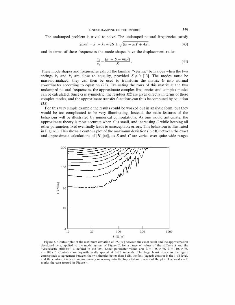
For this very simple example the results could be worked out in analytic form, but theywould be too complicated to be very illuminating. Instead, the main features of thebehaviour will be illustrated by numerical computations. As one would anticipate, theapproximate theory is most accurate when C is small, and increasing C while keeping allother parameters fixed eventually leads to unacceptable errors. This behaviour is illustratedin Figure 3. This shows a contour plot of the maximum deviation (in dB) between the exactand approximate calculations of =H12(v)=, as S and C are varied over quite wide ranges

Figure 3. Contour plot of the maximum deviation of =H12(v)= between the exact result and the approximationdeveloped here, applied to the model system of Figure 2, for a range of values of the stiffness S and the‘‘viscoelastic stiffness’’ C defined in the text. Other parameter values are: k1 =1000 N/m, k2 =1100 N/m,l=100 s−1. Contours are logarithmically spaced at 1-dB intervals. The large blank space in the figurecorresponds to agreement between the two theories better than 1 dB, the first (jagged) contour is the 1-dB level,and the contour levels are monotonically increasing into the top left-hand corner of the plot. The solid circlemarks the case treated in Figure 4.

–180

–90

0

0 5 10 15 20 25 30 35 40 45

Frequency (rad/s)

Ph

ase

(d

egre

es)

–70

–60

–50

–40

–30

–20

–10

(a)

H11

(d

B)

. 560

while k1, k2 and l are held fixed at values given in the caption. This deviation gives areasonable measure of the adequacy of the approximate theory: when the prediction iswithin 1 dB of the exact result for all frequencies the approximate theory is presumablyaccurate enough for all practical purposes, but once the deviation grows to a few dB itbecomes less convincing. The jagged form of the lower contours in Figure 3 arises fromnumerical resolution, together with the fact that the measure calculated is a maximumdeviation, and as parameter values change the frequency at which the maximum deviationoccurs can jump.

The detailed behaviour for a case near the threshold of acceptability is shown inFigure 4. It corresponds to the point marked in Figure 3, close to the 5-dB contour. Itcan be seen that the deviation of =H12(v)= is indeed a good measure of the general behaviourof this case. The phase deviation and the deviations of H11 and H22 all follow similarpatterns. The detailed modal results for this case are as follows: the undamped frequenciesand mode vectors are

v1 =32·2211, u1 =$0·85070·5257%,

Figure 4(a)—(Caption page 562)

–360

–90

–180

–270

0

0 5 10 15 20 25 30 35 40 45

Frequency (rad/s)

Ph

ase

(d

egre

es)

–70

–60

–50

–40

–30

–20

–10

(b)

H12

(d

B)

–80

–90

561

Figure 4(b)—(Caption overleaf )

v2 =35·5219, u2 =$−0·52570·8507%, (45)

and the approximate complex values from equations (30) and (31) are

v1 1 32·2519+0·0956i, u1 1$0·8309−0·0614i0·5577+0·0993i%,

v2 1 36·1194+1·6822i, u2 1$−0·5639−0·1073i0·8271−0·0663i%. (46)

The two modal damping factors are quite different in this case: in terms of Q-factors, givenfor small damping by

Qj 1Re (vj )

2 Im (vj ), (47)

–180

–90

0 5 10 15 20 25 30 35 40 45

Frequency (rad/s)

Ph

ase

(d

egre

es)

–70

–60

–50

–40

–30

–20

–10(c)

H22

(d

B)

0

. 562

Figure 4(c)

Figure 4. Comparisons between exact theory (solid lines) and approximate theory (dashed lines) for the threetransfer functions of the system shown in Figure 2: (a) H11(v); (b) H12(v); (c) H22(v). Parameter values are:k1 =1000 N/m, k2 =1100 N/m, S=100 N/m, C=200 N/m, l=100 s−1.

they are

Q1 1 169, Q2 1 10·7. (48)

The reason is that the coupling spring S is sufficiently strong that the system is within the‘‘veering range’’, with modes involving significant motion of both masses, as shown byequation (45). The lower of these two modes involves motion of the two masses in the samedirection, with little extension of the ‘‘viscoelastic’’ element and hence little damping, butthe higher mode involves motion of the masses in opposite directions, and thus much moredamping. Notice that the corresponding mode shape is also changed quite substantiallyfrom the undamped case: one element has an imaginary part which is 19% of its real part,a significantly complex mode. The approximate theory is near the edge of acceptabilitywhen one mode has a Q-factor of 10, very high damping for most structural vibrationapplications. This gives a strong indication that the approximate theory might be usefulfor a wide range of practical problems. Indeed, it is questionable whether there are manyreal systems with modal Q-factors this low in which the damping obeys a linear modelto the required accuracy.

563

The general features of Figure 3 are now easy to explain. For all values of S, thedeviation increases with increasing C as expected. Less immediately obvious is that for agiven value of C, decreasing S increases the deviation. The reason lies in the ‘‘veering’’phenomenon. The mode shapes of this system are very sensitive to the strength of couplingbetween the two masses: for weak coupling, towards the left of the figure, the modes consist(approximately) of separate oscillation of the two masses, but for stronger coupling,towards the right of the figure, they tend towards symmetric and antisymmetric motionof the masses, as described for the case shown in Figure 4. This strength of coupling arisesfrom the parallel combination of the spring S and the viscoelastic element. If the springis strong, a relatively large force from the viscoelastic element still represents a smallperturbation, and the approximate theory works well. However, if the spring S is weak,the net coupling strength is influenced strongly by the viscoelastic element, and it is notsurprising that the perturbation approximation is less good.

Finally, it should be noted that the omission of the contribution associated with theadditional pole of the damping model has made very little difference to the accuracy ofprediction. Even at very low frequencies, the exact and approximate calculations of allthree transfer functions remain in good agreement in amplitude and phase.

4. IMPLICATIONS FOR EXPERIMENTAL MODAL ANALYSIS

4.1. -

Equations (10) and (22) generalize readily from discrete to continuous systems, the modevectors becoming continuous functions of position in the system and the number of modesbecoming infinite. Thus, any system with small damping which can be described by aRayleigh dissipation function should have transfer functions which are well approximatedby equation (22), and which are described exactly by equation (A9). This fact can be usedto predict the results of measurements designed to find mode shapes.

The most common method of experimental modal analysis involves measuring manytransfer functions, usually with a fixed observation point and exciting the structure at manydifferent points using an impulse hammer. Various computational schemes may be usedto identify the poles of these transfer functions, and then to calculate the spatial variationof the residue of a given pole as the excitation point moves. It is immediately clear fromequation (22) that if damping forces are well-represented by a dissipation matrix, the resultof such a measurement does indeed reveal the complex mode corresponding to the chosenpole, as given by equation (10). Also, for this case the principle of reciprocity betweenexcitation and observing points (or generalized co-ordinates) applies: it does not matterwhether the excitation point or the observation point is moved around.

If a set of measurements satisfies the requirement of reciprocity, a dissipation-matrixmodel of damping is a possible candidate, and one might try to extract the parametersof such a model from the measurements. A natural approach is to determine the complexmode shapes (and the diagonal damping terms) by pole-fitting, then use the simpleexpression (10) to determine the off-diagonal terms of the dissipation matrix C'. This wouldinvolve determining the ‘‘undamped’’ modes from the real part of the measured shapes,then expressing the imaginary part of a given complex mode as a linear combination ofthese undamped modes. The coefficients of such an expression would directly give valuesfor C'kn . If the measurements are truly reciprocal, the matrix C' deduced in this way willautomatically be symmetric. Carrying this procedure through in practice would, of course,raise questions of numerical methods and accuracy which are not explored further here.

Often, complex modes are regarded as simply a nuisance when they appear in a modaltest. However, the analysis of section 2 shows that for a general dissipation matrix,

. 564

complex modes appear at the same order of approximation as complex (i.e., damped)natural frequencies. Only for the special case of proportional damping do the modesremain real in the presence of damping. Necessary and sufficient conditions on thedissipation matrix for this to occur have been given by Caughey and O’Kelly [14].However, the concept of proportional damping seems to be entirely a matter ofmathematical convenience. There is no obvious justification for expecting physical systemsto exhibit this effect, and complex modes should be regarded as the norm.

Tracking the poles of transfer functions is not the only approach to experimentaldetermination of mode shapes. A common alternative is to use a ‘‘full-field’’ visualizationtechnique. Typically the structure would be driven at one or more points, with a sinusoidalexcitation tuned to match a resonant peak. Efforts may be made to suppress nearby modesby making the excitation pattern orthogonal to them. For example, in a system havinga plane of symmetry one might use symmetrically-placed drive points driven in antiphaseto excite antisymmetric modes but not symmetric ones. The response field would then beobserved by, for example, holographic means or scanning laser vibrometry.

Not surprisingly, such a method sometimes shows phase differences between differentpoints on the system. These are often described as ‘‘complex modes’’, but one can nowsee easily that they are not in general the same as the complex modes defined earlier. Asimple counter-example is sufficient. Consider a long, uniform, one-dimensional systemwith uniformly distributed viscous damping, such as a long beam undergoing flexuralvibration when submerged in oil. Such a system has a dissipation matrix with the samediagonal form as the mass matrix, so this is a system with proportional damping [1]. Themodes, defined as the free motion of the system corresponding to a given (complex) naturalfrequency, are still purely real in this case. A particular mode involves a certain vibrationpattern in the rod which decays exponentially in time without phase difference betweendifferent points.

If this system is driven at a point with a real frequency v, in order to make a full-fieldmeasurement, the response pattern will show phase differences. If the rod is long, onewould expect to see traces of outgoing waves from the excitation point, which are notentirely matched by reflected waves to form pure standing waves. The reason can be simplystated in terms of travelling-wave components of the motion: the modes have realwavenumbers but (slightly) complex frequencies. If driven at a real frequency, thewavenumber inevitably becomes slightly complex. The two are directly related via thegroup velocity of the system. This problem could only be circumvented if the excitationwas distributed over the entire system in such a way as to be orthogonal to all the othermodes. But to do that would involve knowing the mode shapes in detail in advance, whichdefeats the point of the measurement.

The conclusion seems to be that such full-field methods, although very powerful forshowing the general character of modes, would require considerable care in interpretationif used to study complex modes and damping models. As an example, consider the practiceof using arrangements of driving to eliminate contributions from nearby modes. Equation(10) shows that, in the presence of off-diagonal damping terms in a dissipation matrixmodel, the main perturbation to a given mode shape comes from an admixture of the othermodes, predominantly those closest in frequency. These contributions are in quadraturewith the original ‘‘undamped’’ component of the mode. So according to this model, thedriving arrangement must eliminate any in-phase contribution of the neighbouring modebut not remove a quadrature component. Apart from the practical difficulties of doing thisreliably, there is a hint of circular logic here: to use this fact deliberately in the design ofthe driving is to assume that a dissipation-matrix model of damping is appropriate at theoutset.

565

4.2.

What happens if the methodology of experimental modal analysis is applied to a systemdescribed by the more general damping model of section 3? The first comment to be madeis that the basic methodology of experimental modal analysis should still be applicable tothis rather general class of systems, since it is based on fitting a fixed set of complex polefrequencies to a set of measured transfer functions, and it was shown from equation (29)that the set of poles associated with structural resonances will be the same in all transferfunctions.

One consequence of equation (35) for experimental modal analysis is that for this generalmodel of damping forces, reciprocity will not necessarily be found. However, if the spatialvariation of the residue of one pole is tracked as the observation point (but not theexcitation point) is varied, the result will accurately reproduce the form of the complexmode corresponding to that pole. No assumption has been made about the form of G'except that its terms are small, so this conclusion remains true in the presence ofgeneralized gyroscopic forces as well as truly dissipative forces. If the internal forces ina given system were to behave as in the example of section 3.3, then reciprocity would hold,and the measurement could be made in the usual way by moving the excitation point.

A thorough experimental study aimed at establishing which damping model wasappropriate to a given system, and determining the relevant parameter values, mightproceed by the following steps. First, tests would be made to check for linearity. Ifnon-sinusoidal response to sinusoidal driving, or amplitude-dependence of measuredtransfer functions, were seen, then there would be little point in trying to fit the fine detailsof a linear model. If the system passes this test, a set of transfer functions would bemeasured. Enough measurements must be made to check carefully for failures ofreciprocity. If reciprocity is verified to sufficient accuracy, the simpler version of the generaldamping model with a symmetric matrix should be expected to hold, and it might eventranspire that a dissipation-matrix model will be adequate.

In any case, the next step is to identify the set of poles, and fit the residues of these polesin all the measured transfer functions. If all the modal Q-factors exceed 20 or so, the resultsof the simple example from section 3.3 suggest that the small-damping approximate theorywill be sufficiently accurate to interpret the results with some confidence. In that case thecomplex mode shapes can be deduced, bearing in mind that if reciprocity does not holdthen results must be deduced from variation of the observation point rather than thedriving point. The final stage is to attempt to invert equations (10) or (31) to deduce theparameters of the damping model.

If a dissipation-matrix model is adequate, then there is in principle just enough dataavailable to determine the full set of parameters. The diagonal terms of the dissipationmatrix are deduced from the complex frequencies, via equation (9). To determine theoff-diagonal terms, it would be necessary to express the complex modes as a linearcombination of the undamped mode shapes, each coefficient of this expansion giving thevalue of one term of the dissipation matrix in normal co-ordinates. The undamped modeshapes would be approximated by the real parts of the complex mode shapes. Ideally, thesewould be checked for orthogonality with respect to the mass matrix, then advantage couldbe taken of this fact to carry out the decomposition of the imaginary parts into a modalsum. To carry out this sequence of steps would be a tall order in terms of computationalaccuracy, but it is certainly conceivable. The final check on whether the dissipation-matrixmodel is valid would be made by checking whether the matrix C'jk deduced was symmetric.Recall that this question is unrelated to the issue of reciprocity: the derivation of equation(10) makes no use of symmetry.

. 566

If the more general linear model of damping is relevant, then things are much moredifficult: there simply is not enough information available, even from a perfectmeasurement, to determine the model completely. The same sequence of steps could befollowed, but there are two problems in the final stage. The first problem is that there isno longer a direct experimental way to deduce the undamped mode shapes. It is conceivablethat this could be overcome by a combination of theoretical modelling and careful dataanalysis, but it would be a very tall order. The second problem is even more serious—evenif the decomposition of complex modes into a linear combination of undamped modescould be carried out, the results would only give very sketchy information about thedamping model. The reason is that each element G'jk is an unknown function of frequency,and all one can deduce from equation (31) is the value of this function sampled at theparticular frequency vk . It seems clear that many different damping models might happento give the same complex value at this particular frequency, and thus be indistinguishableby this measurement method.

Admittedly, this argument has omitted one consideration. If it were possible to findreliably the additional poles associated with the damping model, then the theory ofcomplex functions might in principle allow the frequency-dependent behaviour to bededuced on the assumption that the functions G'jk are all analytic except at isolated poles.However, this seems a very slender hope in practice. Probably, one would need to havesome knowledge of the relevant damping model based on knowledge of the physicalmechanisms operating to resolve the serious ambiguity outlined in the previous paragraph.

It thus appears that measurements confined to a certain frequency bandwidth could befitted equally well by a variety of different damping models. Since all these models fit thefull set of transfer functions well, it is reasonable to ask whether the ambiguity overdamping models is important. Under some circumstances, it might not matter at all. Inthat case, one might as well fit a dissipation-matrix model if the experimentally-determinedmatrix is symmetric within the bounds of experimental accuracy. However, for somepurposes of engineering design the ambiguity about damping models might be quitesignificant, especially if the purpose of the measurements on a structure were to predictthe effect of structural modifications. If the damping model is wrong, the spatial variationof the energy dissipation is probably not represented correctly. Recall that the proposedmeasurements are made in normal co-ordinates, and have to be transformed back to givespatial information. That might lead to quite misleading predictions of the effect of alocalized change to the structure. This issue would merit further study.

5. CONCLUSIONS

The vibration behaviour of systems with linear damping has been analyzed in somedetail, both for the case when the damping forces can be expressed through a dissipationmatrix and for the more general case where nothing is assumed beyond linearity. In bothcases, an approximation of ‘‘small damping’’ was made, and this allowed very simpleexpressions to be calculated for the damped natural frequencies, complex mode shapes andtransfer functions. The formulae for transfer functions follow very closely the familiarresult for undamped systems, giving them considerable intuitive appeal. The approximateforms can be found by simple post-processing of the results of an undamped calculation,such as a finite-element computation. A simple numerical example was presented, forwhich it was found that the approximate results gave satisfactory accuracy over a very widerange of parameter values.

The theory has useful implications for the interpretation of results in experimental modalanalysis. It has been shown that, within the limits of this approximation, it should be

567

possible to determine reliably the correct complex modes of any structure for which themechanism of damping is linear to sufficient accuracy. Furthermore, these complex modeshapes can be analyzed to give information about the damping model. It has been shownthat it is not in general possible to determine the correct damping model for a structureby purely empirical means, but the class of possible models can in principle be identified.The problem is that a damping model is specified by a matrix of frequency-dependentfunctions, but for a given structure each of these functions can only be observed at thefrequency of one particular normal mode, via the residue of the corresponding pole in atransfer function. To resolve this fundamental ambiguity would presumably requiredetailed modelling of the physical mechanisms of damping.

ACKNOWLEDGMENTS

The author is grateful to Professor Robin Langley for the result given in the Appendix,and to him and Professor David Newland for useful discussions on this material.

REFERENCES

1. L R 1897 Theory of Sound (two volumes). New York: Dover Publications; secondedition, 1945 re-issue.

2. C. W. B 1973 Journal of Sound and Vibration 29, 129–153. Material damping: an introductoryreview of mathematical models, measures and experimental techniques.

3. D. R. B 1960 Theory of Linear Viscoelasticity. London: Pergamon Press.4. S. H. C 1970 Journal of Sound and Vibration 11, 3–18. The role of damping in vibration

theory.5. M. H 1962 Journal of the Acoustical Society of America 34, 803–808. Measurements of

absorption coefficients of plates.6. L. C, M. H and E. E. U 1972 Structure-borne Sound. Berlin: Springer-Verlag.7. D. J. E 1984 Modal Testing: Theory and Practice. Taunton: Research Studies Press.8. D. E. N 1989 Mechanical Vibration Analysis and Computation. Harlow: Longman

Scientific and Technical.9. A. B 1995 Journal of Sound and Vibration 184, 59–72. Estimates of errors in the frequency

responses of non-classically damped systems.10. E. S 1968 Simple and Complex Vibratory Systems. Pennsylvania: Pennsylvania State

University Press.11. R. S. L 1997 Personal communication.12. R. H. L and R. G. D J 1995 Theory and Application of Statistical Energy Analysis.

Boston: Butterworth-Heineman.13. N. C. P and C. D. M 1986 Journal of Sound and Vibration 106, 451–463. Comments

on curve veering in eigenvalue problems.14. T. K. C and M. E. J. O’K 1965 Journal of Applied Mechanics 32, 583–588. Classical

normal modes in damped linear dynamic systems.

APPENDIX

Equations (1) can be recast in first-order form (see e.g., reference [8]) as

z=Az+F, (A1)

in terms of the state vector and force vector

z=$yy%, F=$ 0M−1f%,

. 568

and the 2N×2N matrix

A=$ 0−M−1K

I−M−1C%.

Assuming the eigenvalues lj (=ivj ) of this matrix are distinct, each is associated with aright eigenvector v(j)

r and a left eigenvector v(j)l :

Av(j)r = ljv(j)

r , v(j)tl A= ljv(j)t

l

or

AR=RL, LA=LL (A2)

where R has the right eigenvectors as its columns, L has the left eigenvectors as its rows,and L=diag (lj ).

For distinct eigenvalues lj , lk , the left and right eigenvectors are orthogonal:

v(j)tl v(k)

r =0 (j$ k).

If one normalizes so that

v(j)tl v(j)

r =1, (A3)

then

L=R−1. (A4)

Thus, from equation (A2)

A=RLL,

and so from equation (A1)

z=[ivI−A]−1F=[ivRL−RLL]−1F=R diag 0 1iv− lj1LF=0s

2N

j=1

v(j)r v(j)t

l

iv− lj1F. (A5)

This expresses the matrix of transfer functions in partial fraction form, which must nowbe related to equation (22). Note that

v(j)r =$ u(j)

lj u(j)%in terms of the complex modes of the second-order system as defined earlier. Now let

v(j)l =$v(j)

1

v(j)2 %.

Then from equation (A1),

6ljv(j)t1 =−v(j)t

2 M−1Kljv(j)t

2 = v(j)t1 − v(j)t

2 M−1C(A6)

from which it follows that

[l2j M+ ljC+K](M−1v(j)

2 )=0,

569

so that

M−1v(j)2 = ajv(j)

r (A7)

for some scalar multiple aj . The value is determined by the normalization condition (A3).Substitution from (A6) yields

aj =1

lj u(j)tMu(j) − l−1j u(j)tKu(j) . (A8)

Using the second-order governing equation for this mode, this can be re-written

aj =1

2lj u(j)tMu(j) + u(j)tCu(j)

(=1/2ivj for the undamped case with the usual normalization.)Combining equations (A5) and (A7), and recalling that the first-order modes occur in

complex-conjugate pairs with eigenvalues ivk , −iv*k , one obtains

Hmn (v)= sN

k=1

iak6− u(k)m u(k)

n

(v− vk )+

u(k)m *u(k)

n *(v+ v*k )7. (A9)

This is written in a form immediately comparable with equation (22).