A Guide to linear dynamic analysis with DampingThis guide starts from the applications of linear dynamic response and its role in FEA simulation. Fundamental concepts and principles will be introduced such as equations of motion, types of vibration, role of damping in engineering, linear dynamic analyses, etc.

CourtesyofFacultyofMechanicalEngineeringandMechatronics;WestPomeranianUniversityofTechnology,Poland

Page 2

About the Author:

My name is Cyprien Rusu, I am a French CAEengineer who wants to teach the right bases of FEASimulation to designers, engineers and everyoneaspiring to get it right!Hundreds of FEA students followed my free FEAwebinars on Youtube, read my blog articles onfeaforall.com and joined my FEA courses to learnmore and improve their understanding of FEA andbecome better engineers!

I have also taught FEA seminars to FEA engineers from all over theworld…

Do you want to join my free FEA course?

Click on the link below and join the course to get a basicunderstanding of the FEA foundations that you need to have:

Join the free FEA course

Page 2

1. Dynamic Analysis Application

Dynamic analysis is strongly related to vibrations.

Vibrations are generally defined as fluctuations of a mechanical or structural system about an equilibrium position. Vibrations are initiated when an inertia element is displaced from its equilibrium position due to an energy imported to the system through an external source.

Vibrations as the science is one of the first courses where most engineers to apply the knowledge obtained from mathematics and basic engineering science courses to solve practical problems. Solution of practical problems in vibrations requires modeling of physical systems. A system is abstracted from its surroundings. Usually assumptions appropriate to the system are made.

Basic engineering science, mathematics and numerical methods are applied to derive a computer based model.

Vibrations induced by an unbalanced helicopter blade while rotating at high speeds can lead to the blade's failure and catastrophe for the helicopter. Excessive vibrations of pumps, compressors, turbo-machinery, and other industrial machines can induce vibrations of the surrounding structure, leading to inefficient operation of the machines while the noise produced can cause human discomfort.

Vibrations occur in many mechanical and structural systems. Without being controlled, vibrations can lead to catastrophic situations.

Vibrations of machine tools or machine tool chatter can lead to improper machining of parts. Structural failure can occur because of large dynamic stresses developed during earthquakes or even wind induced vibrations.

Figure 1: 1940 Tacoma Narrows Bridge failure

Figure 2: Failed compressor components

Page 3

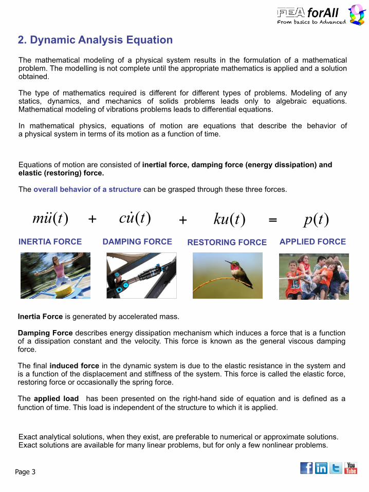
2. Dynamic Analysis Equation

The mathematical modeling of a physical system results in the formulation of a mathematical problem. The modelling is not complete until the appropriate mathematics is applied and a solution obtained. The type of mathematics required is different for different types of problems. Modeling of any statics, dynamics, and mechanics of solids problems leads only to algebraic equations. Mathematical modeling of vibrations problems leads to differential equations.

In mathematical physics, equations of motion are equations that describe the behavior of a physical system in terms of its motion as a function of time.

Exact analytical solutions, when they exist, are preferable to numerical or approximate solutions. Exact solutions are available for many linear problems, but for only a few nonlinear problems.

)(tum !! )(tuc ! )(tku )(tpAPPLIED FORCEINERTIA FORCE DAMPING FORCE RESTORING FORCE

=+ +

Equations of motion are consisted of inertial force, damping force (energy dissipation) and elastic (restoring) force.

The overall behavior of a structure can be grasped through these three forces.

Inertia Force is generated by accelerated mass. Damping Force describes energy dissipation mechanism which induces a force that is a function of a dissipation constant and the velocity. This force is known as the general viscous damping force. The final induced force in the dynamic system is due to the elastic resistance in the system and is a function of the displacement and stiffness of the system. This force is called the elastic force, restoring force or occasionally the spring force. The applied load has been presented on the right-hand side of equation and is defined as a function of time. This load is independent of the structure to which it is applied.

Page 4

2.1 Single Degree of Freedom System

)()()()( tkutuctumtp ++= !!!

2.2 Equation of Motion for Single Degree of Freedom System

System parameters are represented in the model, and their values should be known in order to determine the response of the system to a particular excitation.

State variables are a minimum set of variables, which completely represent the dynamic state of a system at any given time t. For a simple SDOF oscillator an appropriate set of state variables would be the displacement u and the velocity du/dt.

The equation of motion for SDOF mechanical system may be derived using the free-body diagram approach.

Simple mechanical system is schematically shown in Figure 3. The inputs (or excitation) applied to the system are represented by the force p(t). The outputs (or response) of the system are represented by the displacement u(t). The system boundary (real or imaginary) demarcates the region of interest in the analysis. What is outside the system boundary is the environment in which the system operates.

System Response (Outputs)

System Excitation (Inputs)

Environment

Dynamic System State of Variables

Parameters (m, c, k)

System Boundary

u(t)

Figure 3: A Mechanical dynamic system

m – mass c – damping coefficient k – stiffness coefficient p(t) – applied force

Figure 4: SDOF free body diagram.

Page 5

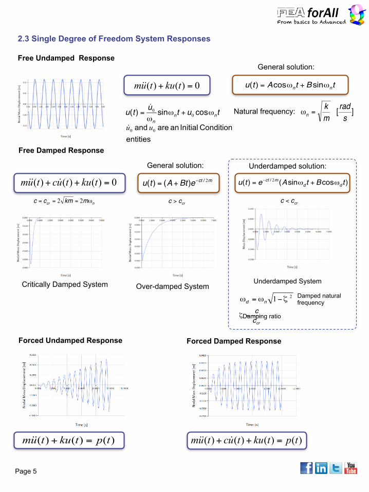
2.3 Single Degree of Freedom System Responses

Free Undamped Response

Free Damped Response

0)()( =+ tkutum !!

)()()( tptkutum =+!! )()()()( tptkutuctum =++ !!!

0)()()( =++ tkutuctum !!!

Forced Undamped Response

tututu nnn

ωωω

cossin)( 00 +=! ][

srad

mk

n =ω

entities Condition Initial an are and 00 uu!

Natural frequency:

mcteBtAtu 2/)()( −+=

Critically Damped System Over-damped SystemUnderdamped System

ncr mkmcc ω22 === crcc >

General solution:

)cossin()( / tBtAetu ddmct ωω += − 2

21 ζωω −= nd

crcc

=ζ

tBtAtu nn ωω sincos)( +=

General solution:

crcc <

Underdamped solution:

Damped natural frequency

Damping ratio

Forced Damped Response

Page 6

3. Dynamic Analysis Types

Structure

Mass StiffnessNatural

Frequencies

Normal Mode Shapes

Analysis of the Normal Modes or Natural Frequencies of a structure is a search for it’s resonant frequencies. By understanding the dynamic characteristics of a structure experiencing oscillation or periodic loads, we can prevents resonance and damage of the structure.

Natural Frequency – the actual measure of frequency, [Hz] or similar units Normal Mode shape – the characteristic deflected shape of a structure as it resonates

Constraints

3.1 Eigenvalue Analysis/Normal Modes/Modal

Load in Time Domain

Structure

Mass Stiffness

Response in Time Domain

Constraints

DampingExecuted in the time domain, it obtains the solution of a dynamic equation of equilibrium when a dynamic load is being applied to a structure.

Though the load and boundary conditions required for a transient response analysis are similar to those of a static analysis, a difference is that load is defined as a function of time.

3.2 Transient Analysis

Load in Freq. Domain

Structure

Mass Stiffness

Response in Freq. Domain

Constraints

DampingA technique to determine the steady state response of a structure according to sinusoidal ( harmonic) loads of known frequency.

Frequency Response is best visualised as a response to a structure on a shaker table. Adjusting the frequency input to the table gives a range of responses.

)sin()()()( tFtkutuctum ω=++ !!!

3.3 Frequency Response Analysis

lead phase frequency driving or input −− ϕω

222

22-1 )/()(

)sin(/)(n

n

tkFtuωζω

ωω

θω

+

+=

Figure 5: SDOF frequency response - Displacement

Figure 6: Shaking table for frequency response experiment

Page 7

4. Dynamic Loading TypesDynamic loads can be applied directly on your model or as time or frequency dependent static loadings.

- Time domain based loading types - Frequency domain based loading types

Figure 8. Dynamic Analysis Solution Types and Methods.

Dynamic Analysis

Direct Integration Method

Modal Superposition Method

Normal Modal Analysis (Eigenvalue Analysis)

Transient Response Analysis Frequency Response Analysis Shock and Response Analysis*

Linear or Nonlinear Analysis

Linear Analysis

*Not Covered in this guide

4.1 Solution MethodsFigure 7. Domain dependent Static Loading.

Page 8

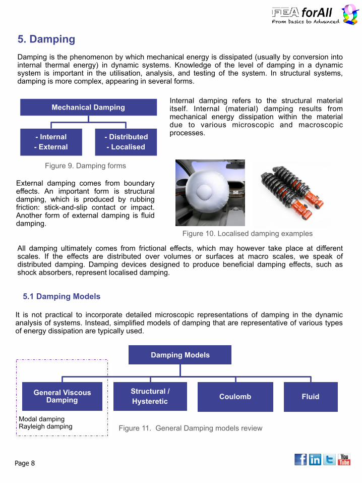
Damping is the phenomenon by which mechanical energy is dissipated (usually by conversion into internal thermal energy) in dynamic systems. Knowledge of the level of damping in a dynamic system is important in the utilisation, analysis, and testing of the system. In structural systems, damping is more complex, appearing in several forms.

5. Damping

Mechanical Damping

- Internal - External

- Distributed - Localised

Damping Models

General Viscous Damping

Structural / Hysteretic Coulomb Fluid

Internal damping refers to the structural material itself. Internal (material) damping results from mechanical energy dissipation within the material due to various microscopic and macroscopic processes.

All damping ultimately comes from frictional effects, which may however take place at different scales. If the effects are distributed over volumes or surfaces at macro scales, we speak of distributed damping. Damping devices designed to produce beneficial damping effects, such as shock absorbers, represent localised damping.

5.1 Damping Models

It is not practical to incorporate detailed microscopic representations of damping in the dynamic analysis of systems. Instead, simplified models of damping that are representative of various types of energy dissipation are typically used.

External damping comes from boundary effects. An important form is structural damping, which is produced by rubbing friction: stick-and-slip contact or impact. Another form of external damping is fluid damping.

Modal damping Rayleigh damping

Figure 10. Localised damping examples

Figure 11. General Damping models review

Figure 9. Damping forms

There are many types of damping: Proportional Damping (Rayleigh; classic)

- Hysteretic/Structural Damping - Direct Damping values - Frequency dependent damping - Modal Damping - Coulomb damping, requires special modelling techniques

Page 9

- BUSH 1D element Property - Damper element Property

- Rayleigh Damping (Proportional)

5.2 Damping Models

5.3 Damping Model input for:

- Structural Damping

- Discrete Viscous Damping

- Defined via Material Card

- Defined via Material Card and Analysis Case Manager

- Overall and Elemental Damping

- Modal Damping- Defined via Analysis Case Manager and Functions

- Coulomb Damping- Defined by combination of elements and

features

Page 10

Various projects require dynamic analysis. Here are a few examples:

6. Dynamic Analysis Project Applications

Mod

e

Frequenc

y1ND 1,046 Hz

2ND 1,778 Hz

3ND 1,801 Hz

4ND 9,457 Hz

5ND 9,679 Hz

6ND 10,217 Hz

In this project, the performance of a cellphone speaker is evaluated under different sound pressure levels.

Displacement / Frequency

Firstly modal analysis was performed to determine natural frequencies of the speaker components. Then frequency response analysis was performed to calculate stresses and deformation shapes of the speaker components according to different frequency spectrums.

From the right image, we can see different mode shapes of the structure. We can also observe that maximum displacement was 0.4 mm, it occurred at around 1000Hz. At this frequency the suspension structure reached its maximum stress of 250MPa.

Stress

Case 2 Resonance avoidance of ultra large AC servo robot

In this case a dynamic characteristics of a servo robot arm was investigated both to avoid resonance during machine operation and to ensure structural safety during earthquakes.

From the image we can confirm the necessity for resonance avoidance design in order to avoid the resonance which happens at 15Hz under repetitive load.

Stresses were equally calculated under seismic load through response spectrum analysis.

Resonance frequency range

Mode Natural Frequency

1st Mode 6.0Hz

2nd Mode 8.2Hz

3rd Mode 14.6Hz

Stress distribution under seismic load

Case 1 Performance evaluation of a mobile speaker through sound pressure level (SPL) analysis

Page 10

Case 3 Brake Disc Squeal Analysis

In this project the dynamic characteristics of brake disc were reviewed to avoid squeal noise caused by vibration. Through frequency response analysis, we can observe that at around 7000 Hz, frequencies of Nodal Diameter Mode and In-Plane Compression Mode are very close, where squeal noise is most likely to occur. Therefore, a design modification is needed to separate 2 frequencies to avoid squealing problems.

Case 4 Safety analysis of marine refrigeration machine under vibration

In this project, natural frequency analysis and frequency response analysis were performed to predict the happening of cracks on the body and piping of a marine refrigeration machine under vibration loads.

ModeNatural

frequency2ND 1027 Hz

3ND 2394 Hz

4ND 3897 Hz

5ND 5468 Hz

1st IPC 7014 Hz

6ND 7045 Hz

7ND 8592 Hz

8ND 10068 Hz

2nd IPC 10285 Hz

1st IPC

6ND

0.0001

0.001

0.01

0.1

1

10

100

0 10 20 30 40 50 60 70 80 90 100Frequency

Frequency Response Function

X-direction

Y-direction

Z-direction

0.0001

0.001

0.01

0.1

1

10

100

0 10 20 30 40 50 60 70 80 90 100Frequency

Frequency Response Function

X-direction

Y-direction

Z-direction

0.0001

0.001

0.01

0.1

1

10

100

0 10 20 30 40 50 60 70 80 90 100Frequency

Frequency Response Function

X-direction

Y-direction

Z-direction

Pipe① Part frequency response Pipe② Part frequency response

Pipe③ Part frequency response

Resonant displacement distribution

1

23

Resonant stress distribution

Do you want to join my free« FEA Foundations » course?

Join the free FEA course

Website:feaforall.comEmail:cyprien@feaforall.comTelephone:+82-31-789-4040

Contact