Linear Algebra

Done Wrong

Sergei Treil

Department of Mathematics, Brown University

Copyright c© Sergei Treil, 2004, 2009

Preface

The title of the book sounds a bit mysterious. Why should anyone read thisbook if it presents the subject in a wrong way? What is particularly done“wrong” in the book?

Before answering these questions, let me first describe the target audi-ence of this text. This book appeared as lecture notes for the course “HonorsLinear Algebra”. It supposed to be a first linear algebra course for math-ematically advanced students. It is intended for a student who, while notyet very familiar with abstract reasoning, is willing to study more rigorousmathematics that is presented in a “cookbook style” calculus type course.Besides being a first course in linear algebra it is also supposed to be afirst course introducing a student to rigorous proof, formal definitions—inshort, to the style of modern theoretical (abstract) mathematics. The targetaudience explains the very specific blend of elementary ideas and concreteexamples, which are usually presented in introductory linear algebra textswith more abstract definitions and constructions typical for advanced books.

Another specific of the book is that it is not written by or for an alge-braist. So, I tried to emphasize the topics that are important for analysis,geometry, probability, etc., and did not include some traditional topics. Forexample, I am only considering vector spaces over the fields of real or com-plex numbers. Linear spaces over other fields are not considered at all, sinceI feel time required to introduce and explain abstract fields would be betterspent on some more classical topics, which will be required in other dis-ciplines. And later, when the students study general fields in an abstractalgebra course they will understand that many of the constructions studiedin this book will also work for general fields.

iii

iv Preface

Also, I treat only finite-dimensional spaces in this book and a basisalways means a finite basis. The reason is that it is impossible to say some-thing non-trivial about infinite-dimensional spaces without introducing con-vergence, norms, completeness etc., i.e. the basics of functional analysis.And this is definitely a subject for a separate course (text). So, I do notconsider infinite Hamel bases here: they are not needed in most applica-tions to analysis and geometry, and I feel they belong in an abstract algebracourse.

Notes for the instructor. There are several details that distinguish thistext from standard advanced linear algebra textbooks. First concerns thedefinitions of bases, linearly independent, and generating sets. In the bookI first define a basis as a system with the property that any vector admitsa unique representation as a linear combination. And then linear indepen-dence and generating system properties appear naturally as halves of thebasis property, one being uniqueness and the other being existence of therepresentation.

The reason for this approach is that I feel the concept of a basis is a muchmore important notion than linear independence: in most applications wereally do not care about linear independence, we need a system to be a basis.For example, when solving a homogeneous system, we are not just lookingfor linearly independent solutions, but for the correct number of linearlyindependent solutions, i.e. for a basis in the solution space.

And it is easy to explain to students, why bases are important: theyallow us to introduce coordinates, and work with Rn (or Cn) instead ofworking with an abstract vector space. Furthermore, we need coordinatesto perform computations using computers, and computers are well adaptedto working with matrices. Also, I really do not know a simple motivationfor the notion of linear independence.

Another detail is that I introduce linear transformations before teach-ing how to solve linear systems. A disadvantage is that we did not proveuntil Chapter 2 that only a square matrix can be invertible as well as someother important facts. However, having already defined linear transforma-tion allows more systematic presentation of row reduction. Also, I spend alot of time (two sections) motivating matrix multiplication. I hope that Iexplained well why such a strange looking rule of multiplication is, in fact,a very natural one, and we really do not have any choice here.

Many important facts about bases, linear transformations, etc., like thefact that any two bases in a vector space have the same number of vectors,are proved in Chapter 2 by counting pivots in the row reduction. While mostof these facts have “coordinate free” proofs, formally not involving Gaussian

Preface v

elimination, a careful analysis of the proofs reveals that the Gaussian elim-ination and counting of the pivots do not disappear, they are just hiddenin most of the proofs. So, instead of presenting very elegant (but not easyfor a beginner to understand) “coordinate-free” proofs, which are typicallypresented in advanced linear algebra books, we use “row reduction” proofs,more common for the “calculus type” texts. The advantage here is that it iseasy to see the common idea behind all the proofs, and such proofs are easierto understand and to remember for a reader who is not very mathematicallysophisticated.

I also present in Section 8 of Chapter 2 a simple and easy to rememberformalism for the change of basis formula.

Chapter 3 deals with determinants. I spent a lot of time presenting amotivation for the determinant, and only much later give formal definitions.Determinants are introduced as a way to compute volumes. It is shown thatif we allow signed volumes, to make the determinant linear in each column(and at that point students should be well aware that the linearity helps alot, and that allowing negative volumes is a very small price to pay for it),and assume some very natural properties, then we do not have any choiceand arrive to the classical definition of the determinant. I would like toemphasize that initially I do not postulate antisymmetry of the determinant;I deduce it from other very natural properties of volume.

Note, that while formally in Chapters 1–3 I was dealing mainly with realspaces, everything there holds for complex spaces, and moreover, even forthe spaces over arbitrary fields.

Chapter 4 is an introduction to spectral theory, and that is where thecomplex space Cn naturally appears. It was formally defined in the begin-ning of the book, and the definition of a complex vector space was also giventhere, but before Chapter 4 the main object was the real space Rn. Nowthe appearance of complex eigenvalues shows that for spectral theory themost natural space is the complex space Cn, even if we are initially dealingwith real matrices (operators in real spaces). The main accent here is on thediagonalization, and the notion of a basis of eigesnspaces is also introduced.

Chapter 5 dealing with inner product spaces comes after spectral theory,because I wanted to do both the complex and the real cases simultaneously,and spectral theory provides a strong motivation for complex spaces. Otherthen the motivation, Chapters 4 and 5 do not depend on each other, and aninstructor may do Chapter 5 first.

Although I present the Jordan canonical form in Chapter 9, I usuallydo not have time to cover it during a one-semester course. I prefer to spendmore time on topics discussed in Chapters 6 and 7 such as diagonalization

vi Preface

of normal and self-adjoint operators, polar and singular values decomposi-tion, the structure of orthogonal matrices and orientation, and the theoryof quadratic forms.

I feel that these topics are more important for applications, then theJordan canonical form, despite the definite beauty of the latter. However, Iadded Chapter 9 so the instructor may skip some of the topics in Chapters6 and 7 and present the Jordan Decomposition Theorem instead.

I also included (new for 2009) Chapter 8, dealing with dual spaces andtensors. I feel that the material there, especially sections about tensors, is abit too advanced for a first year linear algebra course, but some topics (forexample, change of coordinates in the dual space) can be easily included inthe syllabus. And it can be used as an introduction to tensors in a moreadvanced course. Note, that the results presented in this chapter are truefor an arbitrary field.

I had tried to present the material in the book rather informally, prefer-ring intuitive geometric reasoning to formal algebraic manipulations, so toa purist the book may seem not sufficiently rigorous. Throughout the bookI usually (when it does not lead to the confusion) identify a linear transfor-mation and its matrix. This allows for a simpler notation, and I feel thatoveremphasizing the difference between a transformation and its matrix mayconfuse an inexperienced student. Only when the difference is crucial, forexample when analyzing how the matrix of a transformation changes underthe change of the basis, I use a special notation to distinguish between atransformation and its matrix.

Contents

Preface iii

Chapter 1. Basic Notions 1

§1. Vector spaces 1

§2. Linear combinations, bases. 6

§3. Linear Transformations. Matrix–vector multiplication 12

§4. Linear transformations as a vector space 17

§5. Composition of linear transformations and matrix multiplication. 18

§6. Invertible transformations and matrices. Isomorphisms 23

§7. Subspaces. 30

§8. Application to computer graphics. 31

Chapter 2. Systems of linear equations 39

§1. Different faces of linear systems. 39

§2. Solution of a linear system. Echelon and reduced echelon forms 40

§3. Analyzing the pivots. 46

§4. Finding A−1 by row reduction. 52

§5. Dimension. Finite-dimensional spaces. 54

§6. General solution of a linear system. 56

§7. Fundamental subspaces of a matrix. Rank. 59

§8. Representation of a linear transformation in arbitrary bases.Change of coordinates formula. 68

Chapter 3. Determinants 75

vii

viii Contents

§1. Introduction. 75

§2. What properties determinant should have. 76

§3. Constructing the determinant. 78

§4. Formal definition. Existence and uniqueness of the determinant. 86

§5. Cofactor expansion. 89

§6. Minors and rank. 95

§7. Review exercises for Chapter 3. 96

Chapter 4. Introduction to spectral theory (eigenvalues andeigenvectors) 99

§1. Main definitions 100

§2. Diagonalization. 105

Chapter 5. Inner product spaces 115

§1. Inner product in Rn and Cn. Inner product spaces. 115

§2. Orthogonality. Orthogonal and orthonormal bases. 123

§3. Orthogonal projection and Gram-Schmidt orthogonalization 127

§4. Least square solution. Formula for the orthogonal projection 133

§5. Adjoint of a linear transformation. Fundamental subspacesrevisited. 138

§6. Isometries and unitary operators. Unitary and orthogonalmatrices. 142

§7. Rigid motions in Rn 147

§8. Complexification and decomplexification 149

Chapter 6. Structure of operators in inner product spaces. 157

§1. Upper triangular (Schur) representation of an operator. 157

§2. Spectral theorem for self-adjoint and normal operators. 159

§3. Polar and singular value decompositions. 164

§4. What do singular values tell us? 172

§5. Structure of orthogonal matrices 178

§6. Orientation 184

Chapter 7. Bilinear and quadratic forms 189

§1. Main definition 189

§2. Diagonalization of quadratic forms 191

§3. Silvester’s Law of Inertia 196

§4. Positive definite forms. Minimax characterization of eigenvaluesand the Silvester’s criterion of positivity 198

Contents ix

§5. Positive definite forms and inner products 204

Chapter 8. Dual spaces and tensors 207

§1. Dual spaces 207

§2. Dual of an inner product space 214

§3. Adjoint (dual) transformations and transpose. Fundamentalsubspace revisited (once more) 217

§4. What is the difference between a space and its dual? 222

§5. Multilinear functions. Tensors 229

§6. Change of coordinates formula for tensors. 237

Chapter 9. Advanced spectral theory 243

§1. Cayley–Hamilton Theorem 243

§2. Spectral Mapping Theorem 247

§3. Generalized eigenspaces. Geometric meaning of algebraicmultiplicity 249

§4. Structure of nilpotent operators 256

§5. Jordan decomposition theorem 262

Index 265

Chapter 1

Basic Notions

1. Vector spaces

A vector space V is a collection of objects, called vectors (denoted in thisbook by lowercase bold letters, like v), along with two operations, additionof vectors and multiplication by a number (scalar) 1 , such that the following8 properties (the so-called axioms of a vector space) hold:

The first 4 properties deal with the addition:

1. Commutativity: v + w = w + v for all v,w ∈ V ; A question arises,“How one can mem-orize the above prop-erties?” And the an-swer is that one doesnot need to, see be-low!

2. Associativity: (u + v) + w = u + (v + w) for all u,v,w ∈ V ;

3. Zero vector: there exists a special vector, denoted by 0 such thatv + 0 = v for all v ∈ V ;

4. Additive inverse: For every vector v ∈ V there exists a vector w ∈ Vsuch that v + w = 0. Such additive inverse is usually denoted as−v;

The next two properties concern multiplication:

5. Multiplicative identity: 1v = v for all v ∈ V ;

1We need some visual distinction between vectors and other objects, so in this book we usebold lowercase letters for vectors and regular lowercase letters for numbers (scalars). In some (moreadvanced) books Latin letters are reserved for vectors, while Greek letters are used for scalars; in

even more advanced texts any letter can be used for anything and the reader must understandfrom the context what each symbol means. I think it is helpful, especially for a beginner to have

some visual distinction between different objects, so a bold lowercase letters will always denote a

vector. And on a blackboard an arrow (like in ~v) is used to identify a vector.

1

2 1. Basic Notions

6. Multiplicative associativity: (αβ)v = α(βv) for all v ∈ V and allscalars α, β;

And finally, two distributive properties, which connect multipli-cation and addition:

7. α(u + v) = αu + αv for all u,v ∈ V and all scalars α;

8. (α+ β)v = αv + βv for all v ∈ V and all scalars α, β.

Remark. The above properties seem hard to memorize, but it is not nec-essary. They are simply the familiar rules of algebraic manipulations withnumbers, that you know from high school. The only new twist here is thatyou have to understand what operations you can apply to what objects. Youcan add vectors, and you can multiply a vector by a number (scalar). Ofcourse, you can do with number all possible manipulations that you havelearned before. But, you cannot multiply two vectors, or add a number toa vector.

Remark. It is not hard to show that zero vector 0 is unique. It is also easyto show that given v ∈ V the inverse vector −v is unique.

In fact, properties 3 and 4 can be deduced from the properties 5, 6 and8: they imply that 0 = 0v for any v ∈ V , and that −v = (−1)v.

If the scalars are the usual real numbers, we call the space V a realvector space. If the scalars are the complex numbers, i.e. if we can multiplyvectors by complex numbers, we call the space V a complex vector space.

Note, that any complex vector space is a real vector space as well (if wecan multiply by complex numbers, we can multiply by real numbers), butnot the other way around.

It is also possible to consider a situation when the scalars are elementsIf you do not knowwhat a field is, donot worry, since inthis book we con-sider only the caseof real and complexspaces.

of an arbitrary field F. In this case we say that V is a vector space overthe field F. Although many of the constructions in the book (in particular,everything in Chapters 1–3) work for general fields, in this text we consideronly real and complex vector spaces, i.e. F is always either R or C.

Note, that in the definition of a vector space over an arbitrary field, werequire the set of scalars to be a field, so we can always divide (without aremainder) by a non-zero scalar. Thus, it is possible to consider vector spaceover rationals, but not over the integers.

1. Vector spaces 3

1.1. Examples.

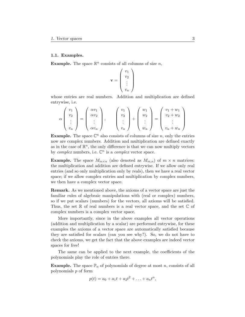
Example. The space Rn consists of all columns of size n,

v =

v1

v2...vn

whose entries are real numbers. Addition and multiplication are definedentrywise, i.e.

α

v1

v2...vn

=

αv1

αv2...

αvn

,

v1

v2...vn

+

w1

w2...wn

=

v1 + w1

v2 + w2...

vn + wn

Example. The space Cn also consists of columns of size n, only the entriesnow are complex numbers. Addition and multiplication are defined exactlyas in the case of Rn, the only difference is that we can now multiply vectorsby complex numbers, i.e. Cn is a complex vector space.

Example. The space Mm×n (also denoted as Mm,n) of m × n matrices:the multiplication and addition are defined entrywise. If we allow only realentries (and so only multiplication only by reals), then we have a real vectorspace; if we allow complex entries and multiplication by complex numbers,we then have a complex vector space.

Remark. As we mentioned above, the axioms of a vector space are just thefamiliar rules of algebraic manipulations with (real or complex) numbers,so if we put scalars (numbers) for the vectors, all axioms will be satisfied.Thus, the set R of real numbers is a real vector space, and the set C ofcomplex numbers is a complex vector space.

More importantly, since in the above examples all vector operations(addition and multiplication by a scalar) are performed entrywise, for theseexamples the axioms of a vector space are automatically satisfied becausethey are satisfied for scalars (can you see why?). So, we do not have tocheck the axioms, we get the fact that the above examples are indeed vectorspaces for free!

The same can be applied to the next example, the coefficients of thepolynomials play the role of entries there.

Example. The space Pn of polynomials of degree at most n, consists of allpolynomials p of form

p(t) = a0 + a1t+ a2t2 + . . .+ ant

n,

4 1. Basic Notions

where t is the independent variable. Note, that some, or even all, coefficientsak can be 0.

In the case of real coefficients ak we have a real vector space, complexcoefficient give us a complex vector space.

Question: What are zero vectors in each of the above examples?

1.2. Matrix notation. An m × n matrix is a rectangular array with mrows and n columns. Elements of the array are called entries of the matrix.

It is often convenient to denote matrix entries by indexed letters: thefirst index denotes the number of the row, where the entry is, and the secondone is the number of the column. For example

(1.1) A = (aj,k)m,j=1,

nk=1 =

a1,1 a1,2 . . . a1,n

a2,1 a2,2 . . . a2,n...

......

am,1 am,2 . . . am,n

is a general way to write an m× n matrix.

Very often for a matrix A the entry in row number j and column numberk is denoted by Aj,k or (A)j,k, and sometimes as in example (1.1) above thesame letter but in lowercase is used for the matrix entries.

Given a matrix A, its transpose (or transposed matrix) AT , is definedby transforming the rows of A into the columns. For example

(1 2 34 5 6

)T=

1 42 53 6

.

So, the columns of AT are the rows of A and vise versa, the rows of AT arethe columns of A.

The formal definition is as follows: (AT )j,k = (A)k,j meaning that the

entry of AT in the row number j and column number k equals the entry ofA in the row number k and row number j.

The transpose of a matrix has a very nice interpretation in terms oflinear transformations, namely it gives the so-called adjoint transformation.We will study this in detail later, but for now transposition will be just auseful formal operation.

One of the first uses of the transpose is that we can write a columnvector x ∈ Rn as x = (x1, x2, . . . , xn)T . If we put the column vertically, itwill use significantly more space.

1. Vector spaces 5

Exercises.

1.1. Let x = (1, 2, 3)T , y = (y1, y2, y3)T , z = (4, 2, 1)T . Compute 2x, 3y, x + 2y−3z.

1.2. Which of the following sets (with natural addition and multiplication by ascalar) are vector spaces. Justify your answer.

a) The set of all continuous functions on the interval [0, 1];

b) The set of all non-negative functions on the interval [0, 1];

c) The set of all polynomials of degree exactly n;

d) The set of all symmetric n × n matrices, i.e. the set of matrices A ={aj,k}nj,k=1 such that AT = A.

1.3. True or false:

a) Every vector space contains a zero vector;

b) A vector space can have more than one zero vector;

c) An m× n matrix has m rows and n columns;

d) If f and g are polynomials of degree n, then f + g is also a polynomial ofdegree n;

e) If f and g are polynomials of degree at most n, then f + g is also apolynomial of degree at most n

1.4. Prove that a zero vector 0 of a vector space V is unique.

1.5. What matrix is the zero vector of the space M2×3?

1.6. Prove that the additive inverse inverse, defined in Axiom 4 of a vector spaceis unique.

6 1. Basic Notions

2. Linear combinations, bases.

Let V be a vector space, and let v1,v2, . . . ,vp ∈ V be a collection of vectors.A linear combination of vectors v1,v2, . . . ,vp is a sum of form

α1v1 + α2v2 + . . .+ αpvp =

p∑k=1

αkvk.

Definition 2.1. A system of vectors v1,v2, . . .vn ∈ V is called a basis (forthe vector space V ) if any vector v ∈ V admits a unique representation asa linear combination

v = α1v1 + α2v2 + . . .+ αnvn =

n∑k=1

αkvk.

The coefficients α1, α2, . . . , αn are called coordinates of the vector v (in thebasis, or with respect to the basis v1,v2, . . . ,vn).

Another way to say that v1,v2, . . . ,vn is a basis is to say that for anypossible choice of the right side v, the equation x1v1 +x2v2 +. . .+xmvn = v(with unknowns xk) has a unique solution.

Before discussing any properties of bases2, let us give few a examples,showing that such objects exist, and that it makes sense to study them.

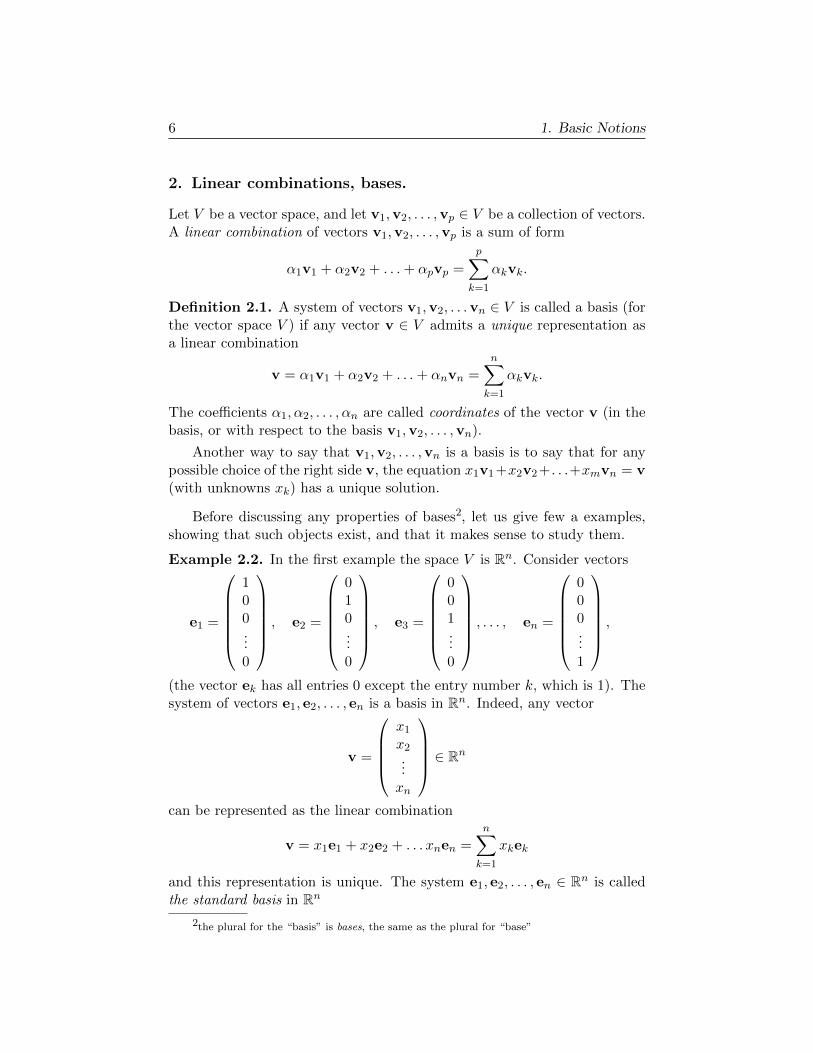
Example 2.2. In the first example the space V is Rn. Consider vectors

e1 =

100...0

, e2 =

010...0

, e3 =

001...0

, . . . , en =

000...1

,

(the vector ek has all entries 0 except the entry number k, which is 1). Thesystem of vectors e1, e2, . . . , en is a basis in Rn. Indeed, any vector

v =

x1

x2...xn

∈ Rn

can be represented as the linear combination

v = x1e1 + x2e2 + . . . xnen =

n∑k=1

xkek

and this representation is unique. The system e1, e2, . . . , en ∈ Rn is calledthe standard basis in Rn

2the plural for the “basis” is bases, the same as the plural for “base”

2. Linear combinations, bases. 7

Example 2.3. In this example the space is the space Pn of the polynomialsof degree at most n. Consider vectors (polynomials) e0, e1, e2, . . . , en ∈ Pndefined by

e0 := 1, e1 := t, e2 := t2, e3 := t3, . . . , en := tn.

Clearly, any polynomial p, p(t) = a0 +a1t+a2t2 + . . .+ant

n admits a uniquerepresentation

p = a0e0 + a1e1 + . . .+ anen.

So the system e0, e1, e2, . . . , en ∈ Pn is a basis in Pn. We will call it thestandard basis in Pn.

Remark 2.4. If a vector space V has a basis v1,v2, . . . ,vn, then any vectorv is uniquely defined by its coefficients in the decomposition v =

∑nk=1 αkvk. This is a very im-

portant remark, thatwill be used through-out the book. It al-lows us to translateany statement aboutthe standard columnspace Rn (or, moregenerally Fn) to avector space V witha basis v1,v2, . . . ,vn

So, if we stack the coefficients αk in a column, we can operate with themas if they were column vectors, i.e. as with elements of Rn (or Fn if V is avector space over a field F; most important cases are F = R of F = C, butthis also works for general fields F).

Namely, if v =∑n

k=1 αkvk and w =∑n

k=1 βkvk, then

v + w =n∑k=1

αkvk +n∑k=1

βkvk =n∑k=1

(αk + βk)vk,

i.e. to get the column of coordinates of the sum one just need to add thecolumns of coordinates of the summands. Similarly, to get the coordinatesof αv we need simply to multiply the column of coordinates of v by α.

2.1. Generating and linearly independent systems. The definitionof a basis says that any vector admits a unique representation as a linearcombination. This statement is in fact two statements, namely that the rep-resentation exists and that it is unique. Let us analyze these two statementsseparately.

If we only consider the existence we get the following notion

Definition 2.5. A system of vectors v1,v2, . . . ,vp ∈ V is called a generatingsystem (also a spanning system, or a complete system) in V if any vectorv ∈ V admits representation as a linear combination

v = α1v1 + α2v2 + . . .+ αpvp =

p∑k=1

αkvk.

The only difference from the definition of a basis is that we do not assumethat the representation above is unique.

8 1. Basic Notions

The words generating, spanning and complete here are synonyms. I per-sonally prefer the term complete, because of my operator theory background.Generating and spanning are more often used in linear algebra textbooks.

Clearly, any basis is a generating (complete) system. Also, if we have abasis, say v1,v2, . . . ,vn, and we add to it several vectors, say vn+1, . . . ,vp,then the new system will be a generating (complete) system. Indeed, we canrepresent any vector as a linear combination of the vectors v1,v2, . . . ,vn,and just ignore the new ones (by putting corresponding coefficients αk = 0).

Now, let us turn our attention to the uniqueness. We do not want toworry about existence, so let us consider the zero vector 0, which alwaysadmits a representation as a linear combination.

Definition. A linear combination α1v1 +α2v2 + . . .+αpvp is called trivialif αk = 0 ∀k.

A trivial linear combination is always (for all choices of vectorsv1,v2, . . . ,vp) equal to 0, and that is probably the reason for the name.

Definition. A system of vectors v1,v2, . . . ,vp ∈ V is called linearly inde-pendent if only the trivial linear combination (

∑pk=1 αkvk with αk = 0 ∀k)

of vectors v1,v2, . . . ,vp equals 0.

In other words, the system v1,v2, . . . ,vp is linearly independent iff theequation x1v1 + x2v2 + . . .+ xpvp = 0 (with unknowns xk) has only trivialsolution x1 = x2 = . . . = xp = 0.

If a system is not linearly independent, it is called linearly dependent.By negating the definition of linear independence, we get the following

Definition. A system of vectors v1,v2, . . . ,vp is called linearly dependentif 0 can be represented as a nontrivial linear combination, 0 =

∑pk=1 αkvk.

Non-trivial here means that at least one of the coefficient αk is non-zero.This can be (and usually is) written as

∑pk=1 |αk| 6= 0.

So, restating the definition we can say, that a system is linearly depen-dent if and only if there exist scalars α1, α2, . . . , αp,

∑pk=1 |αk| 6= 0 such

thatp∑

k=1

αkvk = 0.

An alternative definition (in terms of equations) is that a system v1,v2, . . . ,vp is linearly dependent iff the equation

x1v1 + x2v2 + . . .+ xpvp = 0

(with unknowns xk) has a non-trivial solution. Non-trivial, once again againmeans that at least one of xk is different from 0, and it can be written as∑p

k=1 |xk| 6= 0.

2. Linear combinations, bases. 9

The following proposition gives an alternative description of linearly de-pendent systems.

Proposition 2.6. A system of vectors v1,v2, . . . ,vp ∈ V is linearly de-pendent if and only if one of the vectors vk can be represented as a linearcombination of the other vectors,

(2.1) vk =

p∑j=1j 6=k

βjvj .

Proof. Suppose the system v1,v2, . . . ,vp is linearly dependent. Then thereexist scalars αk,

∑pk=1 |αk| 6= 0 such that

α1v1 + α2v2 + . . .+ αpvp = 0.

Let k be the index such that αk 6= 0. Then, moving all terms except αkvkto the right side we get

αkvk = −p∑j=1j 6=k

αjvj .

Dividing both sides by αk we get (2.1) with βj = −αj/αk.On the other hand, if (2.1) holds, 0 can be represented as a non-trivial

linear combination

vk −p∑j=1j 6=k

βjvj = 0.

�

Obviously, any basis is a linearly independent system. Indeed, if a systemv1,v2, . . . ,vn is a basis, 0 admits a unique representation

0 = α1v1 + α2v2 + . . .+ αnvn =

n∑k=1

αkvk.

Since the trivial linear combination always gives 0, the trivial linear combi-nation must be the only one giving 0.

So, as we already discussed, if a system is a basis it is a complete (gen-erating) and linearly independent system. The following proposition showsthat the converse implication is also true.

Proposition 2.7. A system of vectors v1,v2, . . . ,vn ∈ V is a basis if and In many textbooksa basis is definedas a complete andlinearly independentsystem. By Propo-sition 2.7 this defini-tion is equivalent toours.

only if it is linearly independent and complete (generating).

10 1. Basic Notions

Proof. We already know that a basis is always linearly independent andcomplete, so in one direction the proposition is already proved.

Let us prove the other direction. Suppose a system v1,v2, . . . ,vn is lin-early independent and complete. Take an arbitrary vector v ∈ V . Since thesystem v1,v2, . . . ,vn is linearly complete (generating), v can be representedas

v = α1v1 + α2v2 + . . .+ αnvn =n∑k=1

αkvk.

We only need to show that this representation is unique.

Suppose v admits another representation

v =n∑k=1

αkvk.

Thenn∑k=1

(αk − αk)vk =n∑k=1

αkvk −n∑k=1

αkvk = v − v = 0.

Since the system is linearly independent, αk − αk = 0 ∀k, and thus therepresentation v = α1v1 + α2v2 + . . .+ αnvn is unique. �

Remark. In many textbooks a basis is defined as a complete and linearlyindependent system (by Proposition 2.7 this definition is equivalent to ours).Although this definition is more common than one presented in this text, Iprefer the latter. It emphasizes the main property of a basis, namely thatany vector admits a unique representation as a linear combination.

Proposition 2.8. Any (finite) generating system contains a basis.

Proof. Suppose v1,v2, . . . ,vp ∈ V is a generating (complete) set. If it islinearly independent, it is a basis, and we are done.

Suppose it is not linearly independent, i.e. it is linearly dependent. Thenthere exists a vector vk which can be represented as a linear combination ofthe vectors vj , j 6= k.

Since vk can be represented as a linear combination of vectors vj , j 6= k,any linear combination of vectors v1,v2, . . . ,vp can be represented as a linearcombination of the same vectors without vk (i.e. the vectors vj , 1 ≤ j ≤ p,j 6= k). So, if we delete the vector vk, the new system will still be a completeone.

If the new system is linearly independent, we are done. If not, we repeatthe procedure.

Repeating this procedure finitely many times we arrive to a linearlyindependent and complete system, because otherwise we delete all vectorsand end up with an empty set.

2. Linear combinations, bases. 11

So, any finite complete (generating) set contains a complete linearlyindependent subset, i.e. a basis. �

Exercises.

2.1. Find a basis in the space of 3× 2 matrices M3×2.

2.2. True or false:

a) Any set containing a zero vector is linearly dependent

b) A basis must contain 0;

c) subsets of linearly dependent sets are linearly dependent;

d) subsets of linearly independent sets are linearly independent;

e) If α1v1 + α2v2 + . . .+ αnvn = 0 then all scalars αk are zero;

2.3. Recall, that a matrix is called symmetric if AT = A. Write down a basis in thespace of symmetric 2 × 2 matrices (there are many possible answers). How manyelements are in the basis?

2.4. Write down a basis for the space of

a) 3× 3 symmetric matrices;

b) n× n symmetric matrices;

c) n× n antisymmetric (AT = −A) matrices;

2.5. Let a system of vectors v1,v2, . . . ,vr be linearly independent but not gen-erating. Show that it is possible to find a vector vr+1 such that the systemv1,v2, . . . ,vr,vr+1 is linearly independent. Hint: Take for vr+1 any vector thatcannot be represented as a linear combination

∑rk=1 αkvk and show that the system

v1,v2, . . . ,vr,vr+1 is linearly independent.

2.6. Is it possible that vectors v1,v2,v3 are linearly dependent, but the vectorsw1 = v1 + v2, w2 = v2 + v3 and w3 = v3 + v1 are linearly independent?

12 1. Basic Notions

3. Linear Transformations. Matrix–vector multiplication

A transformation T from a set X to a set Y is a rule that for each argumentThe words “trans-formation”, “trans-form”, “mapping”,“map”, “operator”,“function” all denotethe same object.

(input) x ∈ X assigns a value (output) y = T (x) ∈ Y .

The set X is called the domain of T , and the set Y is called the targetspace or codomain of T .

We write T : X → Y to say that T is a transformation with the domainX and the target space Y .

Definition. Let V , W be vector spaces. A transformation T : V → W iscalled linear if

1. T (u + v) = T (u) + T (v) ∀u,v ∈ V ;

2. T (αv) = αT (v) for all v ∈ V and for all scalars α.

Properties 1 and 2 together are equivalent to the following one:

T (αu + βv) = αT (u) + βT (v) for all u,v ∈ V and for all scalars α, β.

3.1. Examples. You dealt with linear transformation before, may be with-out even suspecting it, as the examples below show.

Example. Differentiation: Let V = Pn (the set of polynomials of degree atmost n), W = Pn−1, and let T : Pn → Pn−1 be the differentiation operator,

T (p) := p′ ∀p ∈ Pn.

Since (f + g)′ = f ′ + g′ and (αf)′ = αf ′, this is a linear transformation.

Example. Rotation: in this example V = W = R2 (the usual coordinateplane), and a transformation Tγ : R2 → R2 takes a vector in R2 and rotatesit counterclockwise by γ radians. Since Tγ rotates the plane as a whole,it rotates as a whole the parallelogram used to define a sum of two vectors(parallelogram law). Therefore the property 1 of linear transformation holds.It is also easy to see that the property 2 is also true.

Example. Reflection: in this example again V = W = R2, and the trans-formation T : R2 → R2 is the reflection in the first coordinate axis, see thefig. It can also be shown geometrically, that this transformation is linear,but we will use another way to show that.

Namely, it is easy to write a formula for T ,

T(( x1

x2

))=

(x1

−x2

)and from this formula it is easy to check that the transformation is linear.

3. Linear Transformations. Matrix–vector multiplication 13

Figure 1. Rotation

Example. Let us investigate linear transformations T : R → R. Any suchtransformation is given by the formula

T (x) = ax where a = T (1).

Indeed,

T (x) = T (x× 1) = xT (1) = xa = ax.

So, any linear transformation of R is just a multiplication by a constant.

3.2. Linear transformations Rn → Rm. Matrix–column multiplica-tion. It turns out that a linear transformation T : Rn → Rm also can berepresented as a multiplication, not by a number, but by a matrix.

Let us see how. Let T : Rn → Rm be a linear transformation. Whatinformation do we need to compute T (x) for all vectors x ∈ Rn? My claimis that it is sufficient to know how T acts on the standard basis e1, e2, . . . , enof Rn. Namely, it is sufficient to know n vectors in Rm (i.e. the vectors ofsize m),

a1 = T (e1), a2 := T (e2), . . . , an := T (en).

14 1. Basic Notions

Indeed, let

x =

x1

x2...xn

.

Then x = x1e1 + x2e2 + . . .+ xnen =∑n

k=1 xkek and

T (x) = T (n∑k=1

xkek) =n∑k=1

T (xkek) =n∑k=1

xkT (ek) =n∑k=1

xkak.

So, if we join the vectors (columns) a1,a2, . . . ,an together in a matrixA = [a1,a2, . . . ,an] (ak being the kth column of A, k = 1, 2, . . . , n), thismatrix contains all the information about T .

Let us show how one should define the product of a matrix and a vector(column) to represent the transformation T as a product, T (x) = Ax. Let

A =

a1,1 a1,2 . . . a1,n

a2,1 a2,2 . . . a2,n...

......

am,1 am,2 . . . am,n

.

Recall, that the column number k of A is the vector ak, i.e.

ak =

a1,k

a2,k...

am,k

.

Then if we want Ax = T (x) we get

Ax =

n∑k=1

xkak = x1

a1,1

a2,1...

am,1

+ x2

a1,2

a2,2...

am,2

+ . . .+ xn

a1,n

a2,n...

am,n

.

So, the matrix–vector multiplication should be performed by the follow-ing column by coordinate rule:

multiply each column of the matrix by the corresponding coordi-nate of the vector.

Example.(1 2 33 2 1

) 123

= 1

(13

)+ 2

(22

)+ 3

(31

)=

(1410

).

3. Linear Transformations. Matrix–vector multiplication 15

The “column by coordinate” rule is very well adapted for parallel com-puting. It will be also very important in different theoretical constructionslater.

However, when doing computations manually, it is more convenient tocompute the result one entry at a time. This can be expressed as the fol-lowing row by column rule:

To get the entry number k of the result, one need to multiply rownumber k of the matrix by the vector, that is, if Ax = y, thenyk =

∑nj=1 ak,jxj , k = 1, 2, . . .m;

here xj and yk are coordinates of the vectors x and y respectively, and aj,kare the entries of the matrix A.

Example.(1 2 34 5 6

) 123

=

(1 · 1 + 2 · 2 + 3 · 34 · 1 + 5 · 2 + 6 · 3

)=

(1432

)

3.3. Linear transformations and generating sets. As we discussedabove, linear transformation T (acting from Rn to Rm) is completely definedby its values on the standard basis in Rn.

The fact that we consider the standard basis is not essential, one canconsider any basis, even any generating (spanning) set. Namely,

A linear transformation T : V → W is completely defined by itsvalues on a generating set (in particular by its values on a basis).

So, if v1,v2, . . . ,vn is a generating set (in particular, if it is a basis) in V ,and T and T1 are linear transformations T, T1 : V →W such that

Tvk = T1vk, k = 1, 2, . . . , n

then T = T1.

3.4. Conclusions.

• To get the matrix of a linear transformation T : Rn → Rm one needsto join the vectors ak = Tek (where e1, e2, . . . , en is the standardbasis in Rn) into a matrix: kth column of the matrix is ak, k =1, 2, . . . , n.

• If the matrix A of the linear transformation T is known, then T (x)can be found by the matrix–vector multiplication, T (x) = Ax. Toperform matrix–vector multiplication one can use either “column bycoordinate” or “row by column” rule.

16 1. Basic Notions

The latter seems more appropriate for manual computations.The former is well adapted for parallel computers, and will be usedin different theoretical constructions.

For a linear transformation T : Rn → Rm, its matrix is usually denotedas [T ]. However, very often people do not distinguish between a linear trans-formation and its matrix, and use the same symbol for both. When it doesnot lead to confusion, we will also use the same symbol for a transformationand its matrix.

Since a linear transformation is essentially a multiplication, the notationThe notation Tv isoften used instead ofT (v).

Tv is often used instead of T (v). We will also use this notation. Note thatthe usual order of algebraic operations apply, i.e. Tv + u means T (v) + u,not T (v + u).

Remark. In the matrix–vector multiplication Ax the number of columnsIn the matrix vectormultiplication usingthe “row by column”rule be sure that youhave the same num-ber of entries in therow and in the col-umn. The entriesin the row and inthe column shouldend simultaneously:if not, the multipli-cation is not defined.

of the matrix A matrix must coincide with the size of the vector x, i.e. avector in Rn can only be multiplied by an m× n matrix.

It makes sense, since an m × n matrix defines a linear transformationRn → Rm, so vector x must belong to Rn.

The easiest way to remember this is to remember that if performingmultiplication you run out of some elements faster, then the multiplicationis not defined. For example, if using the “row by column” rule you runout of row entries, but still have some unused entries in the vector, themultiplication is not defined. It is also not defined if you run out of vector’sentries, but still have unused entries in the row.

Remark. One does not have to restrict himself to the case of Rn withstandard basis: everything described in this section works for transformationbetween arbitrary vector spaces as long as there is a basis in the domain andin the target space. of course, if one changes a basis, the matrix of the lineartransformation will be different. This will be discussed later in Section 8.

Exercises.

3.1. Multiply:

a)

(1 2 34 5 6

) 132

;

b)

1 20 12 0

( 13

);

c)

1 2 0 00 1 2 00 0 1 20 0 0 1

1234

;

4. Linear transformations as a vector space 17

d)

1 2 00 1 20 0 10 0 0

1234

.

3.2. Let a linear transformation in R2 be the reflection in the line x1 = x2. Findits matrix.

3.3. For each linear transformation below find it matrix

a) T : R2 → R3 defined by T (x, y)T = (x+ 2y, 2x− 5y, 7y)T ;

b) T : R4 → R3 defined by T (x1, x2, x3, x4)T = (x1 +x2 +x3 +x4, x2−x4, x1 +3x2 + 6x4)T ;

c) T : Pn → Pn, Tf(t) = f ′(t) (find the matrix with respect to the standardbasis 1, t, t2, . . . , tn);

d) T : Pn → Pn, Tf(t) = 2f(t) + 3f ′(t) − 4f ′′(t) (again with respect to thestandard basis 1, t, t2, . . . , tn).

3.4. Find 3× 3 matrices representing the transformations of R3 which:

a) project every vector onto x-y plane;

b) reflect every vector through x-y plane;

c) rotate the x-y plane through 30◦, leaving z-axis alone.

3.5. Let A be a linear transformation. If z is the center of the straight interval[x, y], show that Az is the center of the interval [Ax,Ay]. Hint: What does it meanthat z is the center of the interval [x, y]?

4. Linear transformations as a vector space

What operations can we perform with linear transformations? We can al-ways multiply a linear transformation for a scalar, i.e. if we have a lineartransformation T : V →W and a scalar α we can define a new transforma-tion αT by

(αT )v = α(Tv) ∀v ∈ V.It is easy to check that αT is also a linear transformation:

(αT )(α1v1 + α2v2) = α(T (α1v1 + α2v2)) by the definition of αT

= α(α1Tv1 + α2Tv2) by the linearity of T

= α1αTv1 + α2αTv2 = α1(αT )v1 + α2(αT )v2

If T1 and T2 are linear transformations with the same domain and targetspace (T1 : V → W and T2 : V → W , or in short T1, T2 : V → W ),then we can add these transformations, i.e. define a new transformationT = (T1 + T2) : V →W by

(T1 + T2)v = T1v + T2v ∀v ∈ V.

18 1. Basic Notions

It is easy to check that the transformation T1 + T2 is a linear one, one justneeds to repeat the above reasoning for the linearity of αT .

So, if we fix vector spaces V and W and consider the collection of alllinear transformations from V to W (let us denote it by L(V,W )), we candefine 2 operations on L(V,W ): multiplication by a scalar and addition.It can be easily shown that these operations satisfy the axioms of a vectorspace, defined in Section 1.

This should come as no surprise for the reader, since axioms of a vectorspace essentially mean that operation on vectors follow standard rules ofalgebra. And the operations on linear transformations are defined as tosatisfy these rules!

As an illustration, let us write down a formal proof of the first distribu-tive law (axiom 7) of a vector space. We want to show that α(T1 + T2) =αT1 + αT2. For any v ∈ V

α(T1 + T2)v = α((T1 + T2)v) by the definition of multiplication

= α(T1v + T2v) by the definition of the sum

= αT1v + αT2v by Axiom 7 for W

= (αT1 + αT2)v by the definition of the sum

So indeed α(T1 + T2) = αT1 + αT2.

Remark. Linear operations (addition and multiplication by a scalar) onlinear transformations T : Rn → Rm correspond to the respective operationson their matrices. Since we know that the set of m× n matrices is a vectorspace, this immediately implies that L(Rn,Rm) is a vector space.

We presented the abstract proof above, first of all because it work forgeneral spaces, for example, for spaces without a basis, where we cannotwork with coordinates. Secondly, the reasonings similar to the abstract onepresented here, are used in many places, so the reader will benefit fromunderstanding it.

And as the reader gains some mathematical sophistication, he/she willsee that this abstract reasoning is indeed a very simple one, that can beperformed almost automatically.

5. Composition of linear transformations and matrixmultiplication.

5.1. Definition of the matrix multiplication. Knowing matrix–vectormultiplication, one can easily guess what is the natural way to define the

5. Composition of linear transformations and matrix multiplication. 19

product AB of two matrices: Let us multiply by A each column of B (matrix-vector multiplication) and join the resulting column-vectors into a matrix.Formally,

if b1,b2, . . . ,br are the columns of B, then Ab1, Ab2, . . . , Abr arethe columns of the matrix AB.

Recalling the row by column rule for the matrix–vector multiplication weget the following row by column rule for the matrices

the entry (AB)j,k (the entry in the row j and column k) of theproduct AB is defined by

(AB)j,k = (row #j of A) · (column #k of B)

Formally it can be rewritten as

(AB)j,k =∑l

aj,lbl,k,

if aj,k and bj,k are entries of the matrices A and B respectively.

I intentionally did not speak about sizes of the matrices A and B, butif we recall the row by column rule for the matrix–vector multiplication, wecan see that in order for the multiplication to be defined, the size of a rowof A should be equal to the size of a column of B.

In other words the product AB is defined if and only if A is an m × nand B is n× r matrix.

5.2. Motivation: composition of linear transformations. One canask yourself here: Why are we using such a complicated rule of multiplica-tion? Why don’t we just multiply matrices entrywise?

And the answer is, that the multiplication, as it is defined above, arisesnaturally from the composition of linear transformations.

Suppose we have two linear transformations, T1 : Rn → Rm and T2 :Rr → Rn. Define the composition T = T1 ◦ T2 of the transformations T1, T2

as

T (x) = T1(T2(x)) ∀x ∈ Rr.Note that T1(x) ∈ Rn. Since T1 : Rn → Rm, the expression T1(T2(x)) is welldefined and the result belongs to Rm. So, T : Rr → Rm. We will usually

identify a lineartransformation andits matrix, but inthe next fewparagraphs we willdistinguish them

It is easy to show that T is a linear transformation (exercise), so it isdefined by an m × r matrix. How one can find this matrix, knowing thematrices of T1 and T2?

Let A be the matrix of T1 and B be the matrix of T2. As we discussed inthe previous section, the columns of T are vectors T (e1), T (e2), . . . , T (er),

20 1. Basic Notions

where e1, e2, . . . , er is the standard basis in Rr. For k = 1, 2, . . . , r we have

T (ek) = T1(T2(ek)) = T1(Bek) = T1(bk) = Abk

(operators T2 and T1 are simply the multiplication by B and A respectively).

So, the columns of the matrix of T are Ab1, Ab2, . . . , Abr, and that isexactly how the matrix AB was defined!

Let us return to identifying again a linear transformation with its matrix.Since the matrix multiplication agrees with the composition, we can (andwill) write T1T2 instead of T1 ◦ T2 and T1T2x instead of T1(T2(x)).

Note that in the composition T1T2 the transformation T2 is applied first!Note: order oftransformations! The way to remember this is to see that in T1T2x the transformation T2

meets x fist.

Remark. There is another way of checking the dimensions of matrices in aproduct, different form the row by column rule: for a composition T1T2 tobe defined it is necessary that T2x belongs to the domain of T1. If T2 actsfrom some space, say Rr to Rn, then T1 must act from Rn to some space,say Rm. So, in order for T1T2 to be defined the matrices of T1 and T2 shouldbe of sizes m × n and n × r respectively—the same condition as obtainedfrom the row by column rule.

Example. Let T : R2 → R2 be the reflection in the line x1 = 3x2. It isa linear transformation, so let us find its matrix. To find the matrix, weneed to compute Te1 and Te2. However, the direct computation of Te1 andTe2 involves significantly more trigonometry than a sane person is willingto remember.

An easier way to find the matrix of T is to represent it as a compositionof simple linear transformation. Namely, let γ be the angle between thex1 axis and the line x1 = 3x2, and let T0 be the reflection in the x1-axis.Then to get the reflection T we can first rotate the plane by the angle −γ,moving the line x1 = 3x2 to the x1-axis, then reflect everything in the x1

axis, and then rotate the plane by γ, taking everything back. Formally itcan be written as

T = RγT0R−γ

(note the order of terms!), where Rγ is the rotation by γ. The matrix of T0

is easy to compute,

T0 =

(1 00 −1

),

5. Composition of linear transformations and matrix multiplication. 21

the rotation matrices are known

Rγ =

(cos γ − sin γsin γ cos γ,

),

R−γ =

(cos(−γ) − sin(−γ)sin(−γ) cos(−γ),

)=

(cos γ sin γ− sin γ cos γ,

)To compute sin γ and cos γ take a vector in the line x1 = 3x2, say a vector(3, 1)T . Then

cos γ =first coordinate

length=

3√32 + 12

=3√10

and similarly

sin γ =second coordinate

length=

1√32 + 12

=1√10

Gathering everything together we get

T = RγT0R−γ =1√10

(3 −11 3

)(1 00 −1

)1√10

(3 1−1 3

)=

1

10

(3 −11 3

)(1 00 −1

)(3 1−1 3

)It remains only to perform matrix multiplication here to get the final result.

�

5.3. Properties of matrix multiplication. Matrix multiplication enjoysa lot of properties, familiar to us from high school algebra:

1. Associativity: A(BC) = (AB)C, provided that either left or rightside is well defined;

2. Distributivity: A(B + C) = AB + AC, (A + B)C = AC + BC,provided either left or right side of each equation is well defined;

3. One can take scalar multiplies out: A(αB) = αAB.

This properties are easy to prove. One should prove the correspondingproperties for linear transformations, and they almost trivially follow fromthe definitions. The properties of linear transformations then imply theproperties for the matrix multiplication.

The new twist here is that the commutativity fails:

matrix multiplication is non-commutative, i.e. generally formatrices AB 6= BA.

One can see easily it would be unreasonable to expect the commutativity ofmatrix multiplication. Indeed, let A and B be matrices of sizes m× n andn× r respectively. Then the product AB is well defined, but if m 6= r, BAis not defined.

22 1. Basic Notions

Even when both products are well defined, for example, when A and Bare n×n (square) matrices, the multiplication is still non-commutative. If wejust pick the matrices A and B at random, the chances are that AB 6= BA:we have to be very lucky to get AB = BA.

5.4. Transposed matrices and multiplication. Given a matrix A, itstranspose (or transposed matrix) AT is defined by transforming the rows ofA into the columns. For example(

1 2 34 5 6

)T=

1 42 53 6

.

So, the columns of AT are the rows of A and vise versa, the rows of AT arethe columns of A.

The formal definition is as follows: (AT )j,k = (A)k,j meaning that the

entry of AT in the row number j and column number k equals the entry ofA in the row number k and row number j.

The transpose of a matrix has a very nice interpretation in terms oflinear transformations, namely it gives the so-called adjoint transformation.We will study this in detail later, but for now transposition will be just auseful formal operation.

One of the first uses of the transpose is that we can write a columnvector x ∈ Rn as x = (x1, x2, . . . , xn)T . If we put the column vertically, itwill use significantly more space.

A simple analysis of the row by columns rule shows that

(AB)T = BTAT ,

i.e. when you take the transpose of the product, you change the order of theterms.

5.5. Trace and matrix multiplication. For a square (n × n) matrixA = (aj,k) its trace (denoted by traceA) is the sum of the diagonal entries

traceA =

n∑k=1

ak,k.

Theorem 5.1. Let A and B be matrices of size m×n and n×m respectively(so the both products AB and BA are well defined). Then

trace(AB) = trace(BA)

We leave the proof of this theorem as an exercise, see Problem 5.6 below.There are essentially two ways of proving this theorem. One is to compute

6. Invertible transformations and matrices. Isomorphisms 23

the diagonal entries of AB and of BA and compare their sums. This methodrequires some proficiency in manipulating sums in

∑notation.

If you are not comfortable with algebraic manipulations, there is anotherway. We can consider two linear transformations, T and T1, acting fromMn×m to R = R1 defined by

T (X) = trace(AX), T1(X) = trace(XA)

To prove the theorem it is sufficient to show that T = T1; the equality forX = B gives the theorem.

Since a linear transformation is completely defined by its values on agenerating system, we need just to check the equality on some simple ma-trices, for example on matrices Xj,k, which has all entries 0 except the entry1 in the intersection of jth column and kth row.

Exercises.

5.1. Let

A =

(1 23 1

), B =

(1 0 23 1 −2

), C =

(1 −2 3−2 1 −1

), D =

−221

a) Mark all the products that are defined, and give the dimensions of the

result: AB, BA, ABC, ABD, BC, BCT , BTC, DC, DTCT .

b) Compute AB, A(3B + C), BTA, A(BD), (AB)D.

5.2. Let Tγ be the matrix of rotation by γ in R2. Check by matrix multiplicationthat TγT−γ = T−γTγ = I

5.3. Multiply two rotation matrices Tα and Tβ (it is a rare case when the multi-plication is commutative, i.e. TαTβ = TβTα, so the order is not essential). Deduceformulas for sin(α+ β) and cos(α+ β) from here.

5.4. Find the matrix of the orthogonal projection in R2 onto the line x1 = −2x2.Hint: What is the matrix of the projection onto the coordinate axis x1?

5.5. Find linear transformations A,B : R2 → R2 such that AB = 0 but BA 6= 0.

5.6. Prove Theorem 5.1, i.e. prove that trace(AB) = trace(BA).

5.7. Construct a non-zero matrix A such that A2 = 0.

5.8. Find the matrix of the reflection through the line y = −2x/3. Perform all themultiplications.

6. Invertible transformations and matrices. Isomorphisms

6.1. Identity transformation and identity matrix. Among all lineartransformations, there is a special one, the identity transformation (opera-tor) I, Ix = x, ∀x.

24 1. Basic Notions

To be precise, there are infinitely many identity transformations: forany vector space V , there is the identity transformation I = I

V: V → V ,

IV

x = x, ∀x ∈ V . However, when it is does not lead to the confusionwe will use the same symbol I for all identity operators (transformations).We will use the notation I

Vonly we want to emphasize in what space the

transformation is acting.

Clearly, if I : Rn → Rn is the identity transformation in Rn, its matrixOften, the symbol Eis used in Linear Al-gebra textbooks forthe identity matrix.I prefer I, since it isused in operator the-ory.

is an n× n matrix

I = In =

1 0 . . . 00 1 . . . 0...

.... . .

...0 0 . . . 1

(1 on the main diagonal and 0 everywhere else). When we want to emphasizethe size of the matrix, we use the notation In; otherwise we just use I.

Clearly, for an arbitrary linear transformation A, the equalities

AI = A, IA = A

hold (whenever the product is defined).

6.2. Invertible transformations.

Definition. Let A : V → W be a linear transformation. We say thatthe transformation A is left invertible if there exist a linear transformationB : W → V such that

BA = I (I = IV

here).

The transformation A is called right invertible if there exists a linear trans-formation C : W → V such that

AC = I (here I = IW

).

The transformations B and C are called left and right inverses of A. Note,that we did not assume the uniqueness of B or C here, and generally leftand right inverses are not unique.

Definition. A linear transformation A : V → W is called invertible if it isboth right and left invertible.

Theorem 6.1. If a linear transformation A : V →W is invertible, then itsleft and right inverses B and C are unique and coincide.

Corollary. A transformation A : V → W is invertible if and only if thereVery often this prop-erty is used as thedefinition of an in-vertible transforma-tion

exists a unique linear transformation (denoted A−1), A−1 : W → V suchthat

A−1A = IV, AA−1 = I

W.

6. Invertible transformations and matrices. Isomorphisms 25

The transformation A−1 is called the inverse of A.

Proof of Theorem 6.1. Let BA = I and AC = I. Then

BAC = B(AC) = BI = B.

On the other hand

BAC = (BA)C = IC = C,

and therefore B = C.

Suppose for some transformation B1 we have B1A = I. Repeating theabove reasoning with B1 instead of B we get B1 = C. Therefore the leftinverse B is unique. The uniqueness of C is proved similarly. �

Definition. A matrix is called invertible (resp. left invertible, right invert-ible) if the corresponding linear transformation is invertible (resp. left in-vertible, right invertible).

Theorem 6.1 asserts that a matrix A is invertible if there exists a uniquematrix A−1 such that A−1A = I, AA−1 = I. The matrix A−1 is called(surprise) the inverse of A.

Examples.

1. The identity transformation (matrix) is invertible, I−1 = I;

2. The rotation Rγ

Rγ =

(cos γ − sin γsin γ cos γ

)is invertible, and the inverse is given by (Rγ)−1 = R−γ . This equalityis clear from the geometric description of Rγ , and it also can bechecked by the matrix multiplication;

3. The column (1, 1)T is left invertible but not right invertible. One ofthe possible left inverses in the row (1/2, 1/2).

To show that this matrix is not right invertible, we just noticethat there are more than one left inverse. Exercise: describe allleft inverses of this matrix.

4. The row (1, 1) is right invertible, but not left invertible. The column(1/2, 1/2)T is a possible right inverse.

Remark 6.2. An invertible matrix must be square (n × n). Moreover, ifa square matrix A has either left of right inverse, it is invertible. So, it is An invertible matrix

must be square (tobe proved later)

sufficient to check only one of the identities AA−1 = I, A−1A = I.

This fact will be proved later. Until we prove this fact, we will not useit. I presented it here only to stop student from trying wrong directions.

26 1. Basic Notions

6.2.1. Properties of the inverse transformation.

Theorem 6.3 (Inverse of the product). If linear transformations A and Bare invertible (and such that the product AB is defined), then the productInverse of a product:

(AB)−1 = B−1A−1.Note the change oforder

AB is invertible and

(AB)−1 = B−1A−1

(note the change of the order!)

Proof. Direct computation shows:

(AB)(B−1A−1) = A(BB−1)A−1 = AIA−1 = AA−1 = I

and similarly

(B−1A−1)(AB) = B−1(A−1A)B = B−1IB = B−1B = I

�

Remark 6.4. The invertibility of the product AB does not imply the in-vertibility of the factors A and B (can you think of an example?). However,if one of the factors (either A or B) and the product AB are invertible, thenthe second factor is also invertible.

We leave the proof of this fact as an exercise.

Theorem 6.5 (Inverse of AT ). If a matrix A is invertible, then AT is alsoinvertible and

(AT )−1 = (A−1)T

Proof. Using (AB)T = BTAT we get

(A−1)TAT = (AA−1)T = IT = I,

and similarly

AT (A−1)T = (A−1A)T = IT = I.

�

And finally, if A is invertible, then A−1 is also invertible, (A−1)−1 = A.

So, let us summarize the main properties of the inverse:

1. If A is invertible, then A−1 is also invertible, (A−1)−1 = A;

2. If A and B are invertible and the product AB is defined, then ABis invertible and (AB)−1 = B−1A−1.

3. If A is invertible, then AT is also invertible and (AT )−1 = (A−1)T .

6. Invertible transformations and matrices. Isomorphisms 27

6.3. Isomorphism. Isomorphic spaces. An invertible linear transfor-mation A : V →W is called an isomorphism. We did not introduce anythingnew here, it is just another name for the object we already studied.

Two vector spaces V and W are called isomorphic (denoted V ∼= W ) ifthere is an isomorphism A : V →W .

Isomorphic spaces can be considered as different representation of thesame space, meaning that all properties and constructions involving vectorspace operations are preserved under isomorphism.

The theorem below illustrates this statement.

Theorem 6.6. Let A : V → W be an isomorphism, and let v1,v2, . . . ,vnbe a basis in V . Then the system Av1, Av2, . . . , Avn is a basis in W .

We leave the proof of the theorem as an exercise.

Remark. In the above theorem one can replace “basis” by “linearly inde-pendent”, or “generating”, or “linearly dependent”—all these properties arepreserved under isomorphisms.

Remark. If A is an isomorphism, then so is A−1. Therefore in the abovetheorem we can state that v1,v2, . . . ,vn is a basis if and only if Av1, Av2,. . . , Avn is a basis.

The inverse to the Theorem 6.6 is also true

Theorem 6.7. Let A : V → W be a linear map,and let v1,v2, . . . ,vn andw1,w2, . . . ,wn are bases in V and W respectively. If Avk = wk, k =1, 2, . . . , n, then A is an isomorphism.

Proof. Define the inverse transformation A−1 by A−1wk = vk, k = 1,2, . . . , n (as we know, a linear transformation is defined by its values on abasis). �

Examples.

1. Let A : Rn+1 → Pn (Pn is the set of polynomials∑n

k=0 aktk of degree

at most n) is defined by

Ae1 = 1, Ae2 = t, . . . , Aen = tn−1, Aen+1 = tn

By Theorem 6.7 A is an isomorphism, so Pn ∼= Rn+1.

2. Let V be a (real) vector space with a basis v1,v2, . . . ,vn. Definetransformation A : Rn → V by Any real vector

space with a basis isisomorphic to Rn .

Aek = vk, k = 1, 2, . . . , n,

where e1, e2, . . . , en is the standard basis in Rn. Again by Theorem6.7 A is an isomorphism, so V ∼= Rn.

28 1. Basic Notions

3. M2×3∼= R6;

4. More generally, Mm×n ∼= Rm·n

6.4. Invertibility and equations.

Theorem 6.8. Let A : X → Y be a linear transformation. Then A isDoesn’t this remindyou of a basis? invertible if and only if for any right side b ∈ Y the equation

Ax = b

has a unique solution x ∈ X.

Proof. Suppose A is invertible. Then x = A−1b solves the equation Ax =b. To show that the solution is unique, suppose that for some other vectorx1 ∈ X

Ax1 = b

Multiplying this identity by A−1 from the left we get

A−1Ax = A−1b,

and therefore x1 = A−1b = x. Note that both identities, AA−1 = I andA−1A = I were used here.

Let us now suppose that the equation Ax = b has a unique solution xfor any b ∈ Y . Let us use symbol y instead of b. We know that given y ∈ Ythe equation

Ax = y

has a unique solution x ∈ X. Let us call this solution B(y).

Note that B(y) is defined for all y ∈ Y , so we defined a transformationB : Y → X.

Let us check that B is a linear transformation. We need to show thatB(αy1+βy2) = αB(y1)+βB(y2). Let xk := B(yk), k = 1, 2, i.e. Axk = yk,k = 1, 2. Then

A(αx1 + βx2) = αAx1 + βAx2 = αy2 + βy2,

which means

B(αy1 + βy2) = αB(y1) + βB(y2).

And finally, let us show that B is indeed the inverse of A. Take x ∈ Xand let y = Ax, so by the definition of B we have x = By. Then for allx ∈ X

BAx = By = x,

so BA = I. Similarly, for arbitrary y ∈ Y let x = By, so y = Ax. Then forall y ∈ Y

ABy = Ax = y

so AB = I. �

6. Invertible transformations and matrices. Isomorphisms 29

Recalling the definition of a basis we get the following corollary of The-orem 6.7.

Corollary 6.9. An m × n matrix is invertible if and only if its columnsform a basis in Rm.

Exercises.

6.1. Prove, that if A : V → W is an isomorphism (i.e. an invertible linear trans-formation) and v1,v2, . . . ,vn is a basis in V , then Av1, Av2, . . . , Avn is a basis inW .

6.2. Find all right inverses to the 1 × 2 matrix (row) A = (1, 1). Conclude fromhere that the row A is not left invertible.

6.3. Find all left inverses of the column (1, 2, 3)T

6.4. Is the column (1, 2, 3)T right invertible? Justify

6.5. Find two matrices A and B that AB is invertible, but A and B are not. Hint:square matrices A and B would not work. Remark: It is easy to construct suchA and B in the case when AB is a 1× 1 matrix (a scalar). But can you get 2× 2matrix AB? 3× 3? n× n?

6.6. Suppose the product AB is invertible. Show that A is right invertible and Bis left invertible. Hint: you can just write formulas for right and left inverses.

6.7. Let A be n× n matrix. Prove that if A2 = 0 then A is not invertible

6.8. Suppose AB = 0 for some non-zero matrix B. Can A be invertible? Justify.

6.9. Write matrices of the linear transformations T1 and T2 in R5, defined as follows:T1 interchanges the coordinates x2 and x4 of the vector x, and T2 just adds to thecoordinate x2 a times the coordinate x4, and does not change other coordinates,i.e.

T1

x1

x2

x3

x4

x5

=

x1

x4

x3

x2

x5

, T2

x1

x2

x3

x4

x5

=

x1

x2 + ax4

x3

x4

x5

;

here a is some fixed number.

Show that T1 and T2 are invertible transformations, and write the matrices ofthe inverses. Hint: it may be simpler, if you first describe the inverse transforma-tion, and then find its matrix, rather than trying to guess (or compute) the inversesof the matrices T1, T2.

6.10. Find the matrix of the rotation in R3 through the angle α around the vector(1, 2, 3)T . We assume that rotation is counterclockwise if we sit at the tip of thevector and looking at the origin.

You can present the answer as a product of several matrices: you don’t haveto perform the multiplication.

6.11. Give examples of matrices (say 2× 2) such that:

30 1. Basic Notions

a) A+B is not invertible although both A and B are invertible;

b) A+B is invertible although both A and B are not invertible;

c) All of A, B and A+B are invertible

6.12. Let A be an invertible symmetric (AT = A) matrix. Is the inverse of Asymmetric? Justify.

7. Subspaces.

A subspace of a vector space V is a non-empty subset V0 ⊂ V of V which isclosed under the vector addition and multiplication by scalars, i.e.

1. If v ∈ V0 then αv ∈ V0 for all scalars α;

2. For any u,v ∈ V0 the sum u + v ∈ V0;

Again, the conditions 1 and 2 can be replaced by the following one:

αu + βv ∈ V0 for all u,v ∈ V0, and for all scalars α, β.

Note, that a subspace V0 ⊂ V with the operations (vector additionand multiplication by scalars) inherited from V , is a vector space. Indeed,because all operations are inherited from the vector space V they mustsatisfy all eight axioms of the vector space. The only thing that couldpossibly go wrong, is that the result of some operation does not belong toV0. But the definition of a subspace prohibits this!

Now let us consider some examples:

1. Trivial subspaces of a space V , namely V itself and {0} (the subspaceconsisting only of zero vector). Note, that the empty set ∅ is not avector space, since it does not contain a zero vector, so it is not asubspace.

With each linear transformation A : V →W we can associate the followingtwo subspaces:

2. The null space, or kernel of A, which is denoted as NullA or KerAand consists of all vectors v ∈ V such that Av = 0

3. The range RanA is defined as the set of all vectors w ∈ W whichcan be represented as w = Av for some v ∈ V .

If A is a matrix, i.e. A : Rm → Rn, then recalling column by coordinate ruleof the matrix–vector multiplication, we can see that any vector w ∈ RanAcan be represented as a linear combination of columns of the matrix A. Thatexplains why the term column space (and notation ColA) is often used forthe range of the matrix. So, for a matrix A, the notation ColA is often usedinstead of RanA.

And now the last example.

8. Application to computer graphics. 31

4. Given a system of vectors v1,v2, . . . ,vr ∈ V its linear span (some-times called simply span) L{v1,v2, . . . ,vr} is the collection of allvectors v ∈ V that can be represented as a linear combinationv = α1v1 + α2v2 + . . . + αrvr of vectors v1,v2, . . . ,vr. The no-tation span{v1,v2, . . . ,vr} is also used instead of L{v1,v2, . . . ,vr}

It is easy to check that in all of these examples we indeed have subspaces.We leave this an an exercise for the reader. Some of the statements will beproved later in the text.

Exercises.

7.1. Let X and Y be subspaces of a vector space V . Prove that X∩Y is a subspaceof V .

7.2. Let V be a vector space. For X,Y ⊂ V the sum X + Y is the collection of allvectors v which can be represented as v = x + y, x ∈ X, y ∈ Y . Show that if Xand Y are subspaces of V , then X + Y is also a subspace.

7.3. Let X be a subspace of a vector space V , and let v ∈ V , v /∈ X. Prove thatif x ∈ X then x + v /∈ X.

7.4. Let X and Y be subspaces of a vector space V . Using the previous exercise,show that X ∪ Y is a subspace if and only if X ⊂ Y or Y ⊂ X.

7.5. What is the smallest subspace of the space of 4 × 4 matrices which containsall upper triangular matrices (aj,k = 0 for all j > k), and all symmetric matrices(A = AT )? What is the largest subspace contained in both of those subspaces?

8. Application to computer graphics.

In this section we give some ideas of how linear algebra is used in computergraphics. We will not go into the details, but just explain some ideas.In particular we explain why manipulation with 3 dimensional images arereduced to multiplications of 4× 4 matrices.

8.1. 2-dimensional manipulation. The x-y plane (more precisely, a rec-tangle there) is a good model of a computer monitor. Any object on amonitor is represented as a collection of pixels, each pixel is assigned a spe-cific color. Position of each pixel is determined by the column and row,which play role of x and y coordinates on the plane. So a rectangle on aplane with x-y coordinates is a good model for a computer screen: and agraphical object is just a collection of points.

Remark. There are two types of graphical objects: bitmap objects, whereevery pixel of an object is described, and vector object, where we describeonly critical points, and graphic engine connects them to reconstruct theobject. A (digital) photo is a good example of a bitmap object: every pixelof it is described. Bitmap object can contain a lot of points, so manipulations

32 1. Basic Notions

with bitmaps require a lot of computing power. Anybody who has editeddigital photos in a bitmap manipulation program, like Adobe Photoshop,knows that one needs quite a powerful computer, and even with modernand powerful computers manipulations can take some time.

That is the reason that most of the objects, appearing on a computerscreen are vector ones: the computer only needs to memorize critical points.For example, to describe a polygon, one needs only to give the coordinatesof its vertices, and which vertex is connected with which. Of course, notall objects on a computer screen can be represented as polygons, some, likeletters, have curved smooth boundaries. But there are standard methodsallowing one to draw smooth curves through a collection of points, for exam-ple Bezier splines, used in PostScript and Adobe PDF (and in many otherformats).

Anyhow, this is the subject of a completely different book, and we willnot discuss it here. For us a graphical object will be a collection of points(either wireframe model, or bitmap) and we would like to show how one canperform some manipulations with such objects.

The simplest transformation is a translation (shift), where each point(vector) v is translated by a, i.e. the vector v is replaced by v + a (nota-tion v 7→ v + a is used for this). Vector addition is very well adapted tocomputers, so the translation is easy to implement.

Note, that the translation is not a linear transformation (if a 6= 0): whileit preserves the straight lines, it does not preserve 0.

All other transformation used in computer graphics are linear. The firstone that comes to mind is rotation. The rotation by γ around the origin 0is given by the multiplication by the rotation matrix Rγ we discussed above,

Rγ =

(cos γ − sin γsin γ cos γ

).

If we want to rotate around a point a, we first need to translate the pictureby −a, moving the point a to 0, then rotate around 0 (multiply by Rγ) andthen translate everything back by a.

Another very useful transformation is scaling, given by a matrix(a 00 b

),

a, b ≥ 0. If a = b it is uniform scaling which enlarges (reduces) an object,preserving its shape. If a 6= b then x and y coordinates scale differently; theobject becomes “taller” or “wider”.

8. Application to computer graphics. 33

Another often used transformation is reflection: for example the matrix(1 00 −1

),

defines the reflection through x-axis.

We will show later in the book, that any linear transformation in R2 canbe represented either as a composition of scaling rotations and reflections.However it is sometimes convenient to consider some different transforma-tions, like the shear transformation, given by the matrix(

1 tanϕ0 1

).

This transformation makes all objects slanted, the horizontal lines remainhorizontal, but vertical lines go to the slanted lines at the angle ϕ to thehorizontal ones.

8.2. 3-dimensional graphics. Three-dimensional graphics is more com-plicated. First we need to be able to manipulate 3-dimensional objects, andthen we need to represent it on 2-dimensional plane (monitor).

The manipulations with 3-dimensional objects is pretty straightforward,we have the same basic transformations: translation, reflection through aplane, scaling, rotation. Matrices of these transformations are very similarto the matrices of their 2× 2 counterparts. For example the matrices 1 0 0

0 1 00 0 −1

,

a 0 00 b 00 0 c

,

cos γ − sin γ 0sin γ cos γ 0

0 0 1

represent respectively reflection through x-y plane, scaling, and rotationaround z-axis.

Note, that the above rotation is essentially 2-dimensional transforma-tion, it does not change z coordinate. Similarly, one can write matrices forthe other 2 elementary rotations around x and around y axes. It will beshown later that a rotation around an arbitrary axis can be represented asa composition of elementary rotations.

So, we know how to manipulate 3-dimensional objects. Let us nowdiscuss how to represent such objects on a 2-dimensional plane. The simplestway is to project it to a plane, say to the x-y plane. To perform suchprojection one just needs to replace z coordinate by 0, the matrix of thisprojection is 1 0 0

0 1 00 0 0

.

34 1. Basic Notions

x

y

z

F

Figure 2. Perspective projection onto x-y plane: F is the center (focalpoint) of the projection

Such method is often used in technical illustrations. Rotating an objectand projecting it is equivalent to looking at it from different points. However,this method does not give a very realistic picture, because it does not takeinto account the perspective, the fact that the objects that are further awaylook smaller.

To get a more realistic picture one needs to use the so-called perspectiveprojection. To define a perspective projection one needs to pick a point (thecenter of projection or the focal point) and a plane to project onto. Theneach point in R3 is projected into a point on the plane such that the point,its image and the center of the projection lie on the same line, see Fig. 2.

This is exactly how a camera works, and it is a reasonable first approx-imation of how our eyes work.

Let us get a formula for the projection. Assume that the focal point is(0, 0, d)T and that we are projecting onto x-y plane, see Fig. 3 a). Considera point v = (x, y, z)T , and let v∗ = (x∗, y∗, 0)T be its projection. Analyzingsimilar triangles see Fig. 3 b), we get that

x∗

d=

x

d− z ,so

x∗ =xd

d− z =x

1− z/d,

and similarly

y∗ =y

1− z/d.

8. Application to computer graphics. 35

x

x∗

z

d−z

(x, y, z)

(x∗, y∗, 0)

x

z

y

(0, 0, d)a) b)

Figure 3. Finding coordinates x∗, y∗ of the perspective projection ofthe point (x, y, z)T .

Note, that this formula also works if z > d and if z < 0: you can draw thecorresponding similar triangles to check it.

Thus the perspective projection maps a point (x, y, z)T to the point(x

1−z/d ,y

1−z/d , 0)T

.

This transformation is definitely not linear (because of z in the denomi-nator). However it is still possible to represent it as a linear transformation.To do this let us introduce the so-called homogeneous coordinates.

In the homogeneous coordinates, every point in R3 is represented by 4coordinates, the last, 4th coordinate playing role of the scaling coefficient.Thus, to get usual 3-dimensional coordinates of the vector v = (x, y, z)T

from its homogeneous coordinates (x1, x2, x3, x4)T one needs to divide allentries by the last coordinate x4 and take the first 3 coordinates 3 (if x4 = 0this recipe does not work, so we assume that the case x4 = 0 correspondsto the point at infinity).

Thus in homogeneous coordinates the vector v∗ can be represented as(x, y, 0, 1−z/d)T , so in homogeneous coordinates the perspective projection

3If we multiply homogeneous coordinates of a point in R2 by a non-zero scalar, we do not

change the point. In other words, in homogeneous coordinates a point in R3 is represented by aline through 0 in R4.

36 1. Basic Notions

is a linear transformation:xy0

1− z/d

=

1 0 0 00 1 0 00 0 0 00 0 −1/d 1

xyz1

.

Note that in the homogeneous coordinates the translation is also a lineartransformation:

x+ a1

y + a2

z + a3

1

=

1 0 0 a1

0 1 0 a2

0 0 1 a3

0 0 0 1

xyz1

.

But what happen if the center of projection is not a point (0, 0, d)T butsome arbitrary point (d1, d2, d3)T . Then we first need to apply the transla-tion by −(d1, d2, 0)T to move the center to (0, 0, d3)T while preserving thex-y plane, apply the projection, and then move everything back translatingit by (d1, d2, 0)T . Similarly, if the plane we project to is not x-y plane, wemove it to the x-y plane by using rotations and translations, and so on.

All these operations are just multiplications by 4 × 4 matrices. Thatexplains why modern graphic cards have 4× 4 matrix operations embeddedin the processor.

Of course, here we only touched the mathematics behind 3-dimensionalgraphics, there is much more. For example, how to determine which parts ofthe object are visible and which are hidden, how to make realistic lighting,shades, etc.

Exercises.

8.1. What vector in R3 has homogeneous coordinates (10, 20, 30, 5)?

8.2. Show that a rotation through γ can be represented as a composition of twoshear-and-scale transformations

T1 =

(1 0

sin γ cos γ

), T2 =

(sec γ − tan γ

0 1

).

In what order the transformations should be taken?

8.3. Multiplication of a 2-vector by an arbitrary 2 × 2 matrix usually requires 4multiplications.

Suppose a 2× 1000 matrix D contains coordinates of 1000 points in R2. Howmany multiplications is required to transform these points using 2 arbitrary 2 × 2matrices A and B. Compare 2 possibilities, A(BD) and (AB)D.

8. Application to computer graphics. 37

8.4. Write 4×4 matrix performing perspective projection to x-y plane with center(d1, d2, d3)T .

8.5. A transformation T in R3 is a rotation about the line y = x+3 in the x-y planethrough an angle γ. Write a 4× 4 matrix corresponding to this transformation.

You can leave the result as a product of matrices.

Chapter 2

Systems of linearequations

1. Different faces of linear systems.

There exist several points of view on what a system of linear equations, or inshort a linear system is. The first, naıve one is, that it is simply a collectionof m linear equations with n unknowns x1, x2, . . . , xn,

a1,1x1 + a1,2x2 + . . . + a1,nxn = b1a2,1x1 + a2,2x2 + . . . + a2,nxn = b2. . .

am,1x1 + am,2x2 + . . . + am,nxn = bm .

To solve the system is to find all n-tuples of numbers x1, x2, . . . , xn whichsatisfy all m equations simultaneously.

If we denote x := (x1, x2, . . . , xn)T ∈ Rn, b = (b1, b2, . . . , bm)T ∈ Rm,and

A =

a1,1 a1,2 . . . a1,n

a2,1 a2,2 . . . a2,n...

......

am,1 am,2 . . . am,n

,

then the above linear system can be written in the matrix form (as a matrix-vector equation)

Ax = b.

To solve the above equation is to find all vectors x ∈ Rn satisfying Ax = b.

39

40 2. Systems of linear equations

And finally, recalling the “column by coordinate” rule of the matrix-vector multiplication, we can write the system as a vector equation

x1a1 + x2a2 + . . .+ xnan = b,

where ak is the kth column of the matrix A, ak = (a1,k, a2,k, . . . , am,k)T ,

k = 1, 2, . . . , n.

Note, these three examples are essentially just different representationsof the same mathematical object.

Before explaining how to solve a linear system, let us notice that it doesnot matter what we call the unknowns, xk, yk or something else. So, allthe information necessary to solve the system is contained in the matrix A,which is called the coefficient matrix of the system and in the vector (rightside) b. Hence, all the information we need is contained in the followingmatrix

a1,1 a1,2 . . . a1,n b1a2,1 a2,2 . . . a2,n b2

......

......

am,1 am,2 . . . am,n bm

which is obtained by attaching the column b to the matrix A. This matrix iscalled the augmented matrix of the system. We will usually put the verticalline separating A and b to distinguish between the augmented matrix andthe coefficient matrix.

2. Solution of a linear system. Echelon and reduced echelonforms

Linear system are solved by the Gauss–Jordan elimination (which is some-times called row reduction). By performing operations on rows of the aug-mented matrix of the system (i.e. on the equations), we reduce it to a simpleform, the so-called echelon form. When the system is in the echelon form,one can easily write the solution.

2.1. Row operations. There are three types of row operations we use:

1. Row exchange: interchange two rows of the matrix;

2. Scaling: multiply a row by a non-zero scalar a;

3. Row replacement: replace a row # k by its sum with a constantmultiple of a row # j; all other rows remain intact;

It is clear that the operations 1 and 2 do not change the set of solutionsof the system; they essentially do not change the system.

2. Solution of a linear system. Echelon and reduced echelon forms 41

As for the operation 3, one can easily see that it does not lose solutions.Namely, let a “new” system be obtained from an “old” one by a row oper-ation of type 3. Then any solution of the “old” system is a solution of the“new” one.

To see that we do not gain anything extra, i.e. that any solution of the“new” system is also a solution of the “old” one, we just notice that rowoperation of type 3 are reversible, i.e. the “old’ system also can be obtainedfrom the “new” one by applying a row operation of type 3 (can you saywhich one?)

2.1.1. Row operations and multiplication by elementary matrices. There isanother, more “advanced” explanation why the above row operations arelegal. Namely, every row operation is equivalent to the multiplication of thematrix from the left by one of the special elementary matrices.

Namely, the multiplication by the matrix

j k

j

k

1...

.... . .

...... 0

1...

.... . . . . . . . . 0 . . . . . . . . . 1

... 1...

.... . .

...... 1

.... . . . . . . . . 1 . . . . . . . . . 0

1

0 . . .

1

just interchanges the rows number j and number k. Multiplication by thematrix

k

1...

. . .... 0

1 0. . . . . . 0 a 0

0 1

0 . . . 00 1

42 2. Systems of linear equations

multiplies the row number k by a. Finally, multiplication by the matrix

j

k

1...

.... . .

...... 0

. . . . . . 1 . . . 0...

. . ....

. . . . . . a . . . 1. . .0

1

adds to the row #k row #j multiplied by a, and leaves all other rows intact.A way to describe

(or to remember)these elementarymatrices: they areobtained from I byapplying thecorresponding rowoperation to it

To see, that the multiplication by these matrices works as advertised,one can just see how the multiplications act on vectors (columns).

Note that all these matrices are invertible (compare with reversibility ofrow operations). The inverse of the first matrix is the matrix itself. To getthe inverse of the second one, one just replaces a by 1/a. And finally, theinverse of the third matrix is obtained by replacing a by −a. To see thatthe inverses are indeed obtained this way, one again can simply check howthey act on columns.

So, performing a row operation on the augmented matrix of the systemAx = b is equivalent to the multiplication of the system (from the left) bya special invertible matrix E. Left multiplying the equality Ax = b by Ewe get that any solution of the equation

Ax = b

is also a solution of

EAx = Eb.

Multiplying this equation (from the left) by E−1 we get that any of itssolutions is a solution of the equation

E−1EAx = E−1Eb,

which is the original equation Ax = b. So, a row operation does not changethe solution set of a system.

2.2. Row reduction. The main step of row reduction consists of threesub-steps:

1. Find the leftmost non-zero column of the matrix;

2. Make sure, by applying row operations of type 1 (row exchange), ifnecessary, that the first (the upper) entry of this column is non-zero.This entry will be called the pivot entry or simply the pivot;

2. Solution of a linear system. Echelon and reduced echelon forms 43

3. “Kill” (i.e. make them 0) all non-zero entries below the pivot byadding (subtracting) an appropriate multiple of the first row fromthe rows number 2, 3, . . . ,m.

We apply the main step to a matrix, then we leave the first row alone andapply the main step to rows 2, . . . ,m, then to rows 3, . . . ,m, etc.

The point to remember is that after we subtract a multiple of a row fromall rows below it (step 3), we leave it alone and do not change it in any way,not even interchange it with another row.

After applying the main step finitely many times (at most m), we getwhat is called the echelon form of the matrix.

2.2.1. An example of row reduction. Let us consider the following linearsystem:

x1 + 2x2 + 3x3 = 13x1 + 2x2 + x3 = 72x1 + x2 + 2x3 = 1

The augmented matrix of the system is 1 2 3 13 2 1 72 1 2 1

Subtracting 3·Row#1 from the second row, and subtracting 2·Row#1 fromthe third one we get: 1 2 3 1

3 2 1 72 1 2 1

−3R1

−2R1

∼

1 2 3 10 −4 −8 40 −3 −4 −1

Multiplying the second row by −1/4 we get 1 2 3 1

0 1 2 −10 −3 −4 −1

Adding 3·Row#2 to the third row we obtain 1 2 3 1

0 1 2 −10 −3 −4 −1

−3R2 ∼

1 2 3 10 1 2 −10 0 2 −4

Now we can use the so called back substitution to solve the system. Namely,from the last row (equation) we get x3 = −2. Then from the second equationwe get

x2 = −1− 2x3 = −1− 2(−2) = 3,

and finally, from the first row (equation)

x1 = 1− 2x2 − 3x3 = 1− 6 + 6 = 1.

44 2. Systems of linear equations

So, the solution is x1 = 1x2 = 3,x3 = −2,

or in vector form

x =

13−2

or x = (1, 3,−2)T . We can check the solution by multiplying Ax, where Ais the coefficient matrix.

Instead of using back substitution, we can do row reduction from downto top, killing all the entries above the main diagonal of the coefficientmatrix: we start by multiplying the last row by 1/2, and the rest is prettyself-explanatory: 1 2 3 1

0 1 2 −10 0 1 −2

−3R3

−2R3 ∼

1 2 0 70 1 0 30 0 1 −2

−2R2

∼

1 0 0 10 1 0 30 0 1 −2

and we just read the solution x = (1, 3,−2)T off the augmented matrix.

We leave it as an exercise to the reader to formulate the algorithm forthe backward phase of the row reduction.

2.3. Echelon form. A matrix is in echelon form if it satisfies the followingtwo conditions:

1. All zero rows (i.e. the rows with all entries equal 0), if any, are belowall non-zero entries.

For a non-zero row, let us call the leftmost non-zero entry the leading entry.Then the second property of the echelon form can be formulated as follows:

2. For any non-zero row its leading entry is strictly to the right of theleading entry in the previous row.

The leading entry in each row in echelon form is also called pivot entry,Pivots: leading(rightmost non-zeroentries) in a row.

or simply pivot, because these entries are exactly the pivots we used in therow reduction.

A particular case of the echelon form is the so-called triangular form.We got this form in our example above. In this form the coefficient matrix issquare (n×n), all its entries on the main diagonal are non-zero, and all the

2. Solution of a linear system. Echelon and reduced echelon forms 45

entries below the main diagonal are zero. The right side, i.e. the rightmostcolumn of the augmented matrix can be arbitrary.

After the backward phase of the row reduction, we get what the so-called reduced echelon form of the matrix: coefficient matrix equal I, as inthe above example, is a particular case of the reduced echelon form.

The general definition is as follows: we say that a matrix is in the reducedechelon form, if it is in the echelon form and

3. All pivot entries are equal 1;

4. All entries above the pivots are 0. Note, that all entries below thepivots are also 0 because of the echelon form.

To get reduced echelon form from echelon form, we work from the bottomto the top and from the right to the left, using row replacement to kill allentries above the pivots.

An example of the reduced echelon form is the system with the coefficientmatrix equal I. In this case, one just reads the solution from the reducedechelon form. In general case, one can also easily read the solution fromthe reduced echelon form. For example, let the reduced echelon form of thesystem (augmented matrix) be 1 2 0 0 0 1

0 0 1 5 0 2

0 0 0 0 1 3

;

here we boxed the pivots. The idea is to move the variables, correspondingto the columns without pivot (the so-called free variables) to the right side.Then we can just write the solution.

x1 = 1− 2x2

x2 is freex3 = 2− 5x4

x4 is freex5 = 3

or in the vector form

x =

1− 2x2

x2

1− 5x4

x4

3

=

10103

+ x2

−21000

+ x4

00−510

One can also find the solution from the echelon form by using back sub-

stitution: the idea is to work from bottom to top, moving all free variablesto the right side.

46 2. Systems of linear equations

Exercises.

2.1. Write the systems of equations below in matrix form and as vector equations:

a)

x1 + 2x2 − x3 = −12x1 + 2x2 + x3 = 13x1 + 5x2 − 2x3 = −1

b)

x1 − 2x2 − x3 = 1

2x1 − 3x2 + x3 = 63x1 − 5x2 = 7x1 + 5x3 = 9

c)

x1 + 2x2 + 2x4 = 6

3x1 + 5x2 − x3 + 6x4 = 172x1 + 4x2 + x3 + 2x4 = 122x1 − 7x3 + 11x4 = 7

d)

x1 − 4x2 − x3 + x4 = 32x1 − 8x2 + x3 − 4x4 = 9−x1 + 4x2 − 2x3 + 5x4 = −6

e)

x1 + 2x2 − x3 + 3x4 = 22x1 + 4x2 − x3 + 6x4 = 5

x2 + 2x4 = 3

f)

2x1 − 2x2 − x3 + 6x4 −2x5 = 1x1 − x2 + x3 + 2x4 −x5 = 2

4x1 − 4x2 + 5x3 + 7x4 −x5 = 6

g)

3x1 − x2 + x3 − x4 + 2x5 = 5x1 − x2 − x3 − 2x4 − x5 = 2

5x1 − 2x2 + x3 − 3x4 + 3x5 = 102x1 − x2 − 2x4 + x5 = 5

Solve the systems. Write the answers in the vector form.

2.2. Find all solutions of the vector equation

x1v1 + x2v2 + x3v3 = 0,

where v1 = (1, 1, 0)T , v2 = (0, 1, 1)T and v3 = (1, 0, 1)T . What conclusion can youmake about linear independence (dependence) of the system of vectors v1,v2,v3?

3. Analyzing the pivots.

All questions about existence of a solution and it uniqueness can be answeredby analyzing pivots in the echelon (reduced echelon) form of the augmentedmatrix of the system. First of all, let us investigate the question of whenis the equation Ax = b inconsistent, i.e. when it does not have a solution.The answer follows immediately, if one just thinks about it:

3. Analyzing the pivots. 47

a system is inconsistent (does not have a solution) if and onlyif there is a pivot in the last column of an echelon form of theaugmented matrix, i.e. iff an echelon form of the augmented matrixhas a row

(0 0 . . . 0 b

), b 6= 0 in it.

Indeed, such a row correspond to the equation 0x1 + 0x2 + . . .+ 0xn = b 6= 0that does not have a solution. If we don’t have such a row, we just makethe reduced echelon form and then read the solution off it.

Now, three more statements. Note, they all deal with the coefficientmatrix, and not with the augmented matrix of the system.

1. A solution (if it exists) is unique iff there are no free variables, thatis if and only if the echelon form of the coefficient matrix has a pivotin every column;

2. Equation Ax = b is consistent for all right sides b if and only if theechelon form of the coefficient matrix has a pivot in every row.

3. Equation Ax = b has a unique solution for any right side b if andonly if echelon form of the coefficient matrix A has a pivot in everycolumn and every row.

The first statement is trivial, because free variables are responsible forall non-uniqueness. I should only emphasize that this statement does notsay anything about the existence.

The second statement is a tiny bit more complicated. If we have a pivotin every row of the coefficient matrix, we cannot have the pivot in the lastcolumn of the augmented matrix, so the system is always consistent, nomatter what the right side b is.

Let us show that if we have a zero row in the echelon form of the coeffi-cient matrix A, then we can pick a right side b such that the system Ax = bis not consistent. Let Ae echelon form of the coefficient matrix A. Then

Ae = EA,

where E is the product of elementary matrices, corresponding to the rowoperations, E = EN , . . . , E2, E1. If Ae has a zero row, then the last row isalso zero. Therefore, if we put be = (0, . . . , 0, 1)T (all entries are 0, exceptthe last one), then the equation

Aex = be

does not have a solution. Multiplying this equation by E−1 from the left,an recalling that E−1Ae = A, we get that the equation

Ax = E−1be

does not have a solution.

48 2. Systems of linear equations

Finally, statement 3 immediately follows from statements 1 and 2. �

From the above analysis of pivots we get several very important corol-laries. The main observation we use is

In echelon form, any row and any column have no more than 1pivot in it (it can have 0 pivots)

3.1. Corollaries about linear independence and bases. Dimension.Questions as to when a system of vectors in Rn is a basis, a linearly inde-pendent or a spanning system, can be easily answered by the row reduction.

Proposition 3.1. Let us have a system of vectors v1,v2, . . . ,vm ∈ Rn, andlet A = [v1,v2, . . . ,vm] be an n × m matrix with columns v1,v2, . . . ,vm.Then

1. The system v1,v2, . . . ,vm is linearly independent iff echelon form ofA has a pivot in every column;

2. The system v1,v2, . . . ,vm is complete in Rn (spanning, generating)iff echelon form of A has a pivot in every row;

3. The system v1,v2, . . . ,vm is a basis in Rn iff echelon form of A hasa pivot in every column and in every row.

Proof. The system v1,v2, . . . ,vm ∈ Rn is linearly independent if and onlyif the equation

x1v1 + x2v2 + . . .+ xmvm = 0

has the unique (trivial) solution x1 = x2 = . . . = xm = 0, or equivalently,the equation Ax = 0 has unique solution x = 0. By statement 1 above, ithappens if and only if there is a pivot in every column of the matrix.

Similarly, the system v1,v2, . . . ,vm ∈ Rn is complete in Rn if and onlyif the equation

x1v1 + x2v2 + . . .+ xmvm = b

has a solution for any right side b ∈ Rn. By statement 2 above, it happensif and only if there is a pivot in every row in echelon form of the matrix.

And finally, the system v1,v2, . . . ,vm ∈ Rn is a basis in Rn if and onlyif the equation

x1v1 + x2v2 + . . .+ xmvm = b

has unique solution for any right side b ∈ Rn. By statement 3 this happensif and only if there is a pivot in every column and in every row of echelonform of A. �

Proposition 3.2. Any linearly independent system of vectors in Rn cannothave more than n vectors in it.

3. Analyzing the pivots. 49

Proof. Let a system v1,v2, . . . ,vm ∈ Rn be linearly independent, and letA = [v1,v2, . . . ,vm] be the n×m matrix with columns v1,v2, . . . ,vm. ByProposition 3.1 echelon form of A must have a pivot in every column, whichis impossible if m > n (number of pivots cannot be more than number ofrows). �

Proposition 3.3. Any two bases in a vector space V have the same numberof vectors in them.

Proof. Let v1,v2, . . . ,vn and w1,w2, . . . ,wm be two different bases in V .Without loss of generality we can assume that n ≤ m. Consider an isomor-phism A : Rn → V defined by

Aek = vk, k = 1, 2, . . . n,

where e1, e2, . . . , en is the standard basis in Rn.

Since A−1 is also an isomorphism, the system

A−1w1, A−1w2, . . . , A

−1wm

is a basis (see Theorem 6.6 in Chapter 1). So it is linearly independent,and by Proposition 3.2, m ≤ n. Together with the assumption n ≤ m thisimplies that m = n. �

The statement below is a particular case of the above proposition.

Proposition 3.4. Any basis in Rn must have exactly n vectors in it.

Proof. This fact follows immediately from the previous proposition, butthere is also a direct proof. Let v1,v2, . . . ,vm be a basis in Rn and let A bethe n×m matrix with columns v1,v2, . . . ,vm. The fact that the system isa basis, means that the equation

Ax = b

has a unique solution for any (all possible) right side b. The existence meansthat there is a pivot in every row (of a reduced echelon form of the matrix),hence the number of pivots is exactly n. The uniqueness mean that there ispivot in every column of the coefficient matrix (its echelon form), so

m = number of columns = number of pivots = n

�

Proposition 3.5. Any spanning (generating) set in Rn must have at leastn vectors.

Proof. Let v1,v2, . . . ,vm be a complete system in Rn, and let A be n×mmatrix with columns v1,v2, . . . ,vm. Statement 2 of Proposition 3.1 implies

50 2. Systems of linear equations

that echelon form of A has a pivot in every row. Since number of pivotscannot exceed the number of columns, n ≤ m. �

3.2. Corollaries about invertible matrices.

Proposition 3.6. A matrix A is invertible if and only if its echelon formhas pivot in every column and every row.

Proof. As it was discussed in the beginning of the section, the equationAx = b has a unique solution for any right side b if and only if the echelonform of A has pivot in every row and every column. But, we know, seeTheorem 6.8 in Chapter 1, that the matrix (linear transformation) A isinvertible if and only if the equation Ax = b has a unique solution for anypossible right side b.

There is also an alternative proof. We know that a matrix is invertibleif and only if its columns form a basis in (see Corollary 6.9 in Section 6.4,Chapter 1). Proposition 3.4 above states that it happens if and only if thereis a pivot in every row and every column. �

The above proposition immediately implies the following

Corollary 3.7. An invertible matrix must be square (n× n).

Proposition 3.8. If a square (n × n) matrix is left invertible, or if it isright right invertible, then it is invertible. In other words, to check theinvertibility of a square matrix A it is sufficient to check only one of theconditions AA−1 = 1, A−1A = I.

Note, that this proposition applies only to square matrices!

Proof. We know that matrix A is invertible if and only if the equationAx = b has a unique solution for any right side b. This happens if and onlyif the echelon form of the matrix A has pivots in every row and in everycolumn.

If a matrix A is left invertible, the equation Ax = 0 has unique solutionx = 0. Indeed, if B is a left inverse of A (i.e. BA = I), and x satisfies

Ax = 0,

then multiplying this identity by B from the left we get x = 0, so thesolution is unique. Therefore, the echelon form of A has pivots in every row.If the matrix A is square (n× n), the echelon form also has pivots in everycolumn, so the matrix is invertible.

If a matrix A is right invertible, and C is its right inverse (AC = I),then for x = Cb, b ∈ Rn

Ax = ACb = Ib = b.

3. Analyzing the pivots. 51

Therefore, for any right side b the equation Ax = b has a solution x = Cb.Thus, echelon form of A has pivots in every row. If A is square, it also hasa pivot in every column, so A is invertible. �

Exercises.

3.1. For what value of b the system 1 2 22 4 61 2 3

x =

14b

has a solution. Find the general solution of the system for this value of b.

3.2. Determine, if the vectors1100

,

1010

,

0011

,

0101

are linearly independent or not.

Do these four vectors span R4? (In other words, is it a generating system?)

3.3. Determine, which of the following systems of vectors are bases in R3:

a) (1, 2,−1)T , (1, 0, 2)T , (2, 1, 1)T ;

b) (−1, 3, 2)T , (−3, 1, 3)T , (2, 10, 2)T ;

c) (67, 13,−47)T , (π,−7.84, 0)T , (3, 0, 0)T .

3.4. Do the polynomials x3 + 2x, x2 + x + 1, x3 + 5 generate (span) P3? Justifyyour answer

3.5. Can 5 vectors in R4 be linearly independent? Justify your answer.

3.6. Prove or disprove: If the columns of a square (n × n) matrix A are linearlyindependent, so are the columns of A2 = AA.

3.7. Prove or disprove: If the columns of a square (n × n) matrix A are linearlyindependent, so are the rows of A3 = AAA.

3.8. Show, that if the equation Ax = 0 has unique solution (i.e. if echelon form ofA has pivot in every column), then A is left invertible. Hint: elementary matricesmay help.Note: It was shown in the text, that if A is left invertible, then the equationAx = 0 has unique solution. But here you are asked to prove the converse of thisstatement, which was not proved.Remark: This can be a very hard problem, for it requires deep understandingof the subject. However, when you understand what to do, the problem becomesalmost trivial.

3.9. Is the reduced echelon form of a matrix unique? Justify your conclusion.

Namely, suppose that by performing some row operations (not necessarily fol-lowing any algorithm) we end up with a reduced echelon matrix. Do we always

52 2. Systems of linear equations

end up with the same matrix, or can we get different ones? Note that we are onlyallowed to perform row operations, the “column operations”’ are forbidden.

Hint: What happens if you start with an invertible matrix? Also, are the pivotsalways in the same columns, or can it be different depending on what row operationsyou perform? If you can tell what the pivot columns are without reverting to rowoperations, then the positions of pivot columns do not depend on them.

4. Finding A−1 by row reduction.

As it was discussed above, an invertible matrix must be square, and its eche-lon form must have pivots in every row and every column. Therefore reducedechelon form of an invertible matrix is the identity matrix I. Therefore,

Any invertible matrix is row equivalent (i.e. can be reduced by rowoperations) to the identity matrix.

Now let us state a simple algorithm of finding the inverse of an n × nmatrix:

1. Form an augmented n×2n matrix (A | I) by writing the n×n identitymatrix right of A;

2. Performing row operations on the augmented matrix transform A tothe identity matrix I;

3. The matrix I that we added will be automatically transformed toA−1;

4. If it is impossible to transform A to the identity by row operations,A is not invertible

There are several possible explanations of the above algorithm. Thefirst, a naıve one, is as follows: we know that (for an invertible A) the vectorA−1b is the solution of the equation Ax = b. So to find the column numberk of A−1 we need to find the solution of Ax = ek, where e1, e2, . . . , en is thestandard basis in Rn. The above algorithm just solves the equations

Ax = ek, k = 1, 2, . . . , n

simultaneously!

Let us also present another, more “advanced” explanation. As we dis-cussed above, every row operation can be realized as a left multiplicationby an elementary matrix. Let E1, E2, . . . , EN be the elementary matricescorresponding to the row operation we performed, and let E = EN · · ·E2E1

4. Finding A−1 by row reduction. 53

be their product.1 We know that the row operations transform A to iden-tity, i.e. EA = I, so E = A−1. But the same row operations transform theaugmented matrix (A | I) to (EA |E) = (I |A−1). �

This “advanced” explanation using elementary matrices implies an im-portant proposition that will be often used later.

Theorem 4.1. Any invertible matrix can be represented as a product ofelementary matrices.

Proof. As we discussed in the previous paragraph, A−1 = EN · · ·E2E1, so

A = (A−1)−1 = E−11 E−1

2 · · ·E−1N .

�

An Example. Suppose we want to find the inverse of the matrix 1 4 −2−2 −7 7

3 11 −6

.

Augmenting the identity matrix to it and performing row reduction we get 1 4 −2 1 0 0−2 −7 7 0 1 0

3 11 −6 0 0 1

+2R1

−3R1

∼

1 4 −2 1 0 00 1 3 2 1 00 −1 0 −3 0 1

+R2

∼

1 4 −2 1 0 00 1 3 2 1 00 0 3 −1 1 1

×3∼

3 12 −6 3 0 00 1 3 2 1 00 0 3 −1 1 1

+2R3

−R3 ∼

Here in the last row operation we multiplied the first row by 3 to avoidfractions in the backward phase of row reduction. Continuing with the rowreduction we get 3 12 0 1 2 2

0 1 0 3 0 −10 0 3 −1 1 1

−12R2

∼

3 0 0 −35 2 140 1 0 3 0 −10 0 3 −1 1 1

Dividing the first and the last row by 3 we get the inverse matrix −35/3 2/3 14/3

3 0 −1−1/3 1/3 1/3

1Although it does not matter here, but please notice, that if the row operation E1 was

performed first, E1 must be the rightmost term in the product

54 2. Systems of linear equations

Exercises.

4.1. Find the inverse of the matrices 1 2 13 7 32 3 4

,

1 −1 21 1 −21 1 4

.

Show all steps

5. Dimension. Finite-dimensional spaces.

Definition. The dimension dimV of a vector space V is the number ofvectors in a basis.

For a vector space consisting only of zero vector 0 we put dimV = 0. IfV does not have a (finite) basis, we put dimV =∞.

If dimV is finite, we call the space V finite-dimensional; otherwise wecall it infinite-dimensional

Proposition 3.3 asserts that the dimension is well defined, i.e. that itdoes not depend on the choice of a basis.

Proposition 2.8 from Chapter 1 states that any finite spanning systemin a vector space V contains a basis. This immediately implies the following

Proposition 5.1. A vector space V is finite-dimensional if and only if ithas a finite spanning system.

Suppose, that we have a system of vectors in a finite-dimensional vectorspace, and we want to check if it is a basis (or if it is linearly independent,or if it is complete)? Probably the simplest way is to use an isomorphismA : V → Rn, n = dimE to move the problem to Rn, where all such questionscan be answered by row reduction (studying pivots).

Note, that if dimV = n, then there always exists an isomorphism A :V → Rn. Indeed, if dimV = n then there exists a basis v1,v2, . . . ,vn ∈ V ,and one can define an isomorphism A : V → Rn by

Avk = ek, k = 1, 2, . . . , n.

As an example, let us give the following two corollaries of the abovePropositions 3.2, 3.5:

Proposition 5.2. Any linearly independent system in a finite-dimensionalvector space V cannot have more than dimV vectors in it.

Proof. Let v1,v2, . . . ,vm ∈ V be a linearly independent system, and letA : V → Rn be an isomorphism. Then Av1, Av2, . . . , Avm is a linearlyindependent system in Rn, and by Proposition 3.2 m ≤ n. �

5. Dimension. Finite-dimensional spaces. 55

Proposition 5.3. Any generating system in a finite-dimensional vectorspace V must have at least dimV vectors in it.

Proof. Let v1,v2, . . . ,vm ∈ V be a complete system in V , and let A : V →Rn be an isomorphism. Then Av1, Av2, . . . , Avm is a complete system inRn, and by Proposition 3.5 m ≥ n. �

5.1. Completing a linearly independent system to a basis. The fol-lowing statement will play an important role later.

Proposition 5.4 (Completion to a basis). A linearly independent systemof vectors in a finite-dimensional space can be completed to a basis, i.e. ifv1,v2, . . . ,vr are linearly independent vectors in a finite-dimensional vectorspace V then one can find vectors vr+1,vr+2 . . . ,vn such that the system ofvectors v1,v2, . . . ,vn is a basis in V .

Proof. Let n = dimV and let r < n (if r = n then the system v1,v2, . . . ,vris already a basis, and the case r > n is impossible). Take any vector notbelonging to span{v1,v2, . . . ,vr} and call it vr+1 (one can always do thatbecause the system v1,v2, . . . ,vr is not generating). By Exercise 2.5 fromChapter 1 the system v1,v2, . . . ,vr,vr+1 is linearly independent. Repeatthe procedure with the new system to get vector vr+2, and so on.

We will stop the process when we get a generating system. Note, thatthe process cannot continue infinitely, because a linearly independent systemof vectors in V cannot have more than n = dimV vectors. �

Exercises.

5.1. True or false:

a) Every vector space that is generated by a finite set has a basis;

b) Every vector space has a (finite) basis;

c) A vector space cannot have more than one basis;

d) If a vector space has a finite basis, then the number of vectors in everybasis is the same.

e) The dimension of Pn is n;

f) The dimension on Mm×n is m+ n;

g) If vectors v1,v2, . . . ,vn generate (span) the vector space V , then everyvector in V can be written as a linear combination of vector v1,v2, . . . ,vnin only one way;

h) Every subspace of a finite-dimensional space is finite-dimensional;

i) If V is a vector space having dimension n, then V has exactly one subspaceof dimension 0 and exactly one subspace of dimension n.

5.2. Prove that if V is a vector space having dimension n, then a system of vectorsv1,v2, . . . ,vn in V is linearly independent if and only if it spans V .

56 2. Systems of linear equations

5.3. Prove that a linearly independent system of vectors v1,v2, . . . ,vn in a vectorspace V is a basis if and only if n = dimV .

5.4. (An old problem revisited: now this problem should be easy) Is it possible thatvectors v1,v2,v3 are linearly dependent, but the vectors w1 = v1+v2, w2 = v2+v3

and w3 = v3 + v1 are linearly independent? Hint: What dimension the subspacespan(v1,v2,v3) can have?

5.5. Let vectors u,v,w be a basis in V . Show that u + v + w, v + w, w is also abasis in V .

5.6. Consider in the space R5 vectors v1 = (2,−1, 1, 5,−3)T , v2 = (3,−2, 0, 0, 0)T ,v3 = (1, 1, 50,−921, 0)T .

a) Prove that vectors are linearly independent

b) Complete this system of vectors to a basis

If you do part b) first you can do everything without any computations.

6. General solution of a linear system.

In this short section we discuss the structure of the general solution (i.e. ofthe solution set) of a linear system.

We call a system Ax = b homogeneous, if the right side, b = 0, i.e. ahomogeneous system is a system of form Ax = 0.

With each systemAx = b

we can associate a homogeneous system just by putting b = 0.

Theorem 6.1 (General solution of a linear equation). Let a vector x1 satisfythe equation Ax = b, and let H be the set of all solutions of the associatedhomogeneous system

Ax = 0.

Then the set{x = x1 + xh : xh ∈ H}

is the set of all solutions of the equation Ax = b.

In other words, this theorem can be stated as

General solutionof Ax = b

=A particular solu-tion of Ax = b

+General solutionof Ax = 0

.

Proof. Fix a vector x1 satisfying Ax1 = b. Let a vector xh satisfy Axh

= 0.Then for x = x1 + xh we have

Ax = A(x1 + xh) = Ax1 +Axh = b + 0 = b,

so any x of formx = x1 + xh, xh ∈ H

6. General solution of a linear system. 57

is a solution of Ax = b.

Now let x be satisfy Ax = b. Then for xh := x− x1 we get

Axh = A(x− x1) = Ax−Ax1 = b− b = 0,

so xh ∈ H. Therefore any solution x of Ax = b can be represented asx = x1 + xh with some xh ∈ H. �

The power of this theorem is in its generality. It applies to all linearequations, we do not have to assume here that vector spaces are finite-dimensional. You will meet this theorem in differential equations, integralequations, partial differential equations, etc. Besides showing the struc-ture of the solution set, this theorem allows one to separate investigationof uniqueness from the study of existence. Namely, to study uniqueness,we only need to analyze uniqueness of the homogeneous equation Ax = 0,which always has a solution.

There is an immediate application in this course: this theorem allows usto check a solution of a system Ax = b. For example, consider a system

2 3 1 4 −91 1 1 1 −31 1 1 2 −52 2 2 3 −8

x =

176814

.

Performing row reduction one can find the solution of this system

(6.1) x =

31020

+ x3

−21100

+ x5

2−1021

, x3, x5 ∈ R.

The parameters x3, x5 can be denoted here by any other letters, t and s, forexample; we keeping notation x3 and x5 here only to remind us that theycame from the corresponding free variables.

Now, let us suppose, that we are just given this solution, and we wantto check whether or not it is correct. Of course, we can repeat the rowoperations, but this is too time consuming. Moreover, if the solution wasobtained by some non-standard method, it can look differently from whatwe get from the row reduction. For example the formula

(6.2) x =

31020

+ s

−21100

+ t

00121

, s, t ∈ R

58 2. Systems of linear equations

gives the same set as (6.1) (can you say why?); here we just replaced the lastvector in (6.1) by its sum with the second one. So, this formula is differentfrom the solution we got from the row reduction, but it is neverthelesscorrect.

The simplest way to check that (6.1) and (6.2) give us correct solutions,is to check that the first vector (3, 1, 0, 2, 0)T satisfies the equation Ax = b,and that the other two (the ones with the parameters x3 and x5 or s and t infront of them) should satisfy the associated homogeneous equation Ax = 0.

If this checks out, we will be assured that any vector x defined by (6.1)or (6.2) is indeed a solution.

Note, that this method of checking the solution does not guarantee that(6.1) (or (6.2)) gives us all the solutions. For example, if we just somehowmiss the term with x2, the above method of checking will still work fine.

So, how can we guarantee, that we did not miss any free variable, andthere should not be extra term in (6.1)?

What comes to mind, is to count the pivots again. In this example, ifone does row operations, the number of pivots is 3. So indeed, there shouldbe 2 free variables, and it looks like we did not miss anything in (6.1).

To be able to prove this, we will need new notions of fundamental sub-spaces and of rank of a matrix. I should also mention, that in this particularexample, one does not have to perform all row operations to check that thereare only 2 free variables, and that formulas (6.1) and (6.2) both give correctgeneral solution.

Exercises.

6.1. True or false

a) Any system of linear equations has at least one solution;

b) Any system of linear equations has at most one solution;

c) Any homogeneous system of linear equations has at least one solution;

d) Any system of n linear equations in n unknowns has at least one solution;

e) Any system of n linear equations in n unknowns has at most one solution;

f) If the homogeneous system corresponding to a given system of a linearequations has a solution, then the given system has a solution;

g) If the coefficient matrix of a homogeneous system of n linear equations inn unknowns is invertible, then the system has no non-zero solution;

h) The solution set of any system of m equations in n unknowns is a subspacein Rn;

i) The solution set of any homogeneous system of m equations in n unknownsis a subspace in Rn.

7. Fundamental subspaces of a matrix. Rank. 59

6.2. Find a 2 × 3 system (2 equations with 3 unknowns) such that its generalsolution has a form 1

10

+ s

121

, s ∈ R.

7. Fundamental subspaces of a matrix. Rank.

As we discussed above in Section 7 of Chapter 1, with any linear transfor-mation A : V → W we can associate two subspaces, namely, its kernel, ornull space

KerA = NullA := {v ∈ V : Av = 0} ⊂ V,and its range

RanA = {w ∈W : w = Av for some v ∈ V } ⊂W.In other words, the kernel KerA is the solution set of the homogeneousequation Ax = 0, and the range RanA is exactly the set of all right sidesb ∈W for which the equation Ax = b has a solution.

If A is an m× n matrix, i.e. a mapping from Rn to Rm, then it followsfrom the “column by coordinate” rule of the matrix multiplication that anyvector w ∈ RanA can be represented as a linear combination of columns ofA. This explains the name column space (notation ColA), which is oftenused instead of RanA.

If A is a matrix, then in addition to RanA and KerA one can alsoconsider the range and kernel for the transposed matrix AT . Often the termrow space is used for RanAT and the term left null space is used for KerAT

(but usually no special notation is introduced).

The four subspaces RanA, KerA, RanAT , KerAT are called the funda-mental subspaces of the matrix A. In this section we will study importantrelations between the dimensions of the four fundamental subspaces.

We will need the following definition, which is one of the fundamentalnotions of Linear Algebra

Definition. Given a linear transformation (matrix) A its rank, rankA, isthe dimension of the range of A

rankA := dim RanA.

7.1. Computing fundamental subspaces and rank. To compute thefundamental subspaces and rank of a matrix, one needs to do echelon re-duction. Namely, let A be the matrix, and Ae be its echelon form

1. The pivot columns of the original matrix A (i.e. the columns whereafter row operations we will have pivots in the echelon form) give usa basis (one of many possible) in RanA.

60 2. Systems of linear equations

2. The pivot rows of the echelon from Ae give us a basis in the rowspace. Of course, it is possible just to transpose the matrix, andthen do row operations. But if we already have the echelon form ofA, say by computing RanA, then we get RanAT for free.

3. To find a basis in the null space KerA one needs to solve the homo-geneous equation Ax = 0: the details will be seen from the examplebelow.

Example. Consider a matrix1 1 2 2 12 2 1 1 13 3 3 3 21 1 −1 −1 0

.

Performing row operations we get the echelon form1 1 2 2 1

0 0 −3 −3 −1

0 0 0 0 00 0 0 0 0

(the pivots are boxed here). So, the columns 1 and 3 of the original matrix,i.e. the columns

1231

,

223−1

give us a basis in RanA. We also get a basis for the row space RanAT forfree: the first and second row of the echelon form of A, i.e. the vectors

11221

,

00−3−3−1

(we put the vectors vertically here. The question of whether to put vectorshere vertically as columns, or horizontally as rows is is really a matter ofconvention. Our reason for putting them vertically is that although we callRanAT the row space we define it as a column space of AT )

To compute the basis in the null space KerA we need to solve the equa-tion Ax = 0. Compute the reduced echelon form of A, which in this example

7. Fundamental subspaces of a matrix. Rank. 61

is 1 1 0 0 1/3

0 0 1 1 1/30 0 0 0 00 0 0 0 0

.

Note, that when solving the homogeneous equation Ax = 0, it is not neces-sary to write the whole augmented matrix, it is sufficient to work with thecoefficient matrix. Indeed, in this case the last column of the augmentedmatrix is the column of zeroes, which does not change under row opera-tions. So, we can just keep this column in mind, without actually writingit. Keeping this last zero column in mind, we can read the solution off thereduced echelon form above:

x1 = −x2 − 13x5,

x2 is free,x3 = −x4 − 1

3x5

x4 is free,x5 is free,

or, in the vector form

(7.1) x =

−x2 − 1

3x5

x2

−x4 − 13x5

x4

x5

= x2

−11000

+ x4

00−110

+ x5

−1/3

0−1/3

01

The vectors at each free variable, i.e. in our case the vectors

−11000

,

00−110

,

−1/3

0−1/3

01

form a basis in KerA.

Unfortunately, there is no shortcut for finding a basis in KerAT , onemust solve the equation ATx = 0. The knowledge of the echelon form of Adoes not help here.

7.2. Explanation of the computing bases in the fundamental sub-spaces. So, why do the above methods indeed give us bases in the funda-mental subspaces?

62 2. Systems of linear equations

7.2.1. The null space KerA. The case of the null space KerA is probablythe simplest one: since we solved the equation Ax = 0, i.e. found all thesolutions, then any vector in KerA is a linear combination of the vectors weobtained. Thus, the vectors we obtained form a spanning system in KerA.To see that the system is linearly independent, let us multiply each vectorby the corresponding free variable and add everything, see (7.1). Then foreach free variable xk, the entry number k of the resulting vector is exactlyxk, see (7.1) again, so the only way this vector (the linear combination) canbe 0 is when all free variables are 0.

7.2.2. The column space RanA. Let us now explain why the method forfinding a basis in the column space RanA works. First of all, notice thatthe pivot columns of the reduced echelon form Are of A form a basis inRanAre (not in the column space of the original matrix, but of its reducedechelon form!). Since row operations are just left multiplications by invert-ible matrices, they do not change linear independence. Therefore, the pivotcolumns of the original matrix A are linearly independent.

Let us now show that the pivot columns of A span the column spaceof A. Let v1,v2, . . . ,vr be the pivot columns of A, and let v be an arbi-trary column of A. We want to show that v can be represented as a linearcombination of the pivot columns v1,v2, . . . ,vr,

v = α1v1 + α2v2 + . . .+ αrvr.

the reduced echelon form Are is obtained from A by the left multiplication

Are = EA,

where E is a product of elementary matrices, so E is an invertible matrix.The vectors Ev1, Ev2, . . . , Evr are the pivot columns of Are, and the columnv of A is transformed to the column Ev of Are. Since the pivot columnsof Are form a basis in RanAre, vector Ev can be represented as a linearcombination

Ev = α1Ev1 + α2Ev2 + . . .+ αrEvr.

Multiplying this equality by E−1 from the left we get the representation

v = α1v1 + α2v2 + . . .+ αrvr,

so indeed the pivot columns of A span RanA.

7.2.3. The row space RanAT . It is easy to see that the pivot rows of theechelon form Ae of A are linearly independent. Indeed, let w1,w2, . . . ,wr

be the transposed (since we agreed always to put vectors vertically) pivotrows of Ae. Suppose

α1w1 + α2w2 + . . .+ αrwr = 0.

7. Fundamental subspaces of a matrix. Rank. 63

Consider the first non-zero entry of w1. Since for all other vectorsw2,w3, . . . ,wr the corresponding entries equal 0 (by the definition of eche-lon form), we can conclude that α1 = 0. So we can just ignore the first termin the sum.

Consider now the first non-zero entry of w2. The corresponding entriesof the vectors w3, . . . ,wr are 0, so α2 = 0. Repeating this procedure, weget that αk = 0 ∀k = 1, 2, . . . , r.

To see that vectors w1,w2, . . . ,wr span the row space, one can noticethat row operations do not change the row space. This can be obtaineddirectly from analyzing row operations, but we present here a more formalway to demonstrate this fact.

For a transformation A and a set X let us denote by A(X) the set of allelements y which can represented as y = A(x), x ∈ X,

A(X) := {y = A(x) : x ∈ X} .

If A is an m×n matrix, and Ae is its echelon form, Ae is obtained fromA be left multiplication

Ae = EA,

where E is an m ×m invertible matrix (the product of the correspondingelementary matrices). Then

RanATe = Ran(ATET ) = AT (RanET ) = AT (Rm) = RanAT ,

so indeed RanAT = RanATe .

7.3. The Rank Theorem. Dimensions of fundamental subspaces.There are many applications in which one needs to find a basis in columnspace or in the null space of a matrix. For example, as it was shown above,solving a homogeneous equation Ax = 0 amounts to finding a basis inthe null space KerA. Finding a basis in the column space means simplyextracting a basis from a spanning set, by removing unnecessary vectors(columns).

However, the most important application of the above methods of com-puting bases of fundamental subspaces is the relations between their dimen-sions.

Theorem 7.1 (The Rank Theorem). For a matrix A

rankA = rankAT .

This theorem is often stated as follows:

The column rank of a matrix coincides with its row rank.

64 2. Systems of linear equations

The proof of this theorem is trivial, since dimensions of both RanA andRanAT are equal to the number of pivots in the echelon form of A.

The following theorem is gives us important relations between dimen-sions of the fundamental spaces. It is often also called the Rank Theorem

Theorem 7.2. Let A be an m×n matrix, i.e. a linear transformation fromRn to Rm. Then

1. dim KerA+ dim RanA = dim KerA+ rankA = n (dimension of thedomain of A);

2. dim KerAT + dim RanAT = dim KerAT + rankAT =dim KerAT + rankA = m (dimension of the target space of A);

Proof. The proof, modulo the above algorithms of finding bases in thefundamental subspaces, is almost trivial. The first statement is simply thefact that the number of free variables (dim KerA) plus the number of basicvariables (i.e. the number of pivots, i.e. rankA) adds up to the number ofcolumns (i.e. to n).

The second statement, if one takes into account that rankA = rankAT

is simply the first statement applied to AT . �

As an application of the above theorem, let us recall the example fromSection 6. There we considered a system

2 3 1 4 −91 1 1 1 −31 1 1 2 −52 2 2 3 −8

x =

176814

,

and we claimed that its general solution given by

x =

31020

+ x3

−21100

+ x5

2−1021

, x3, x5 ∈ R,

or by

x =

31020

+ s

−21100

+ t

00121

, s, t ∈ R.

We checked in Section 6 that a vector x given by either formula is indeeda solution of the equation. But, how can we guarantee that any of theformulas describe all solutions?

7. Fundamental subspaces of a matrix. Rank. 65

First of all, we know that in either formula, the last 2 vectors (the onesmultiplied by the parameters) belong to KerA. It is easy to see that ineither case both vectors are linearly independent (two vectors are linearlydependent if and only if one is a multiple of the other).

Now, let us count dimensions: interchanging the first and the secondrows and performing first round of row operations

−2R1

−R1

−2R1

1 1 1 1 −32 3 1 4 −91 1 1 2 −52 2 2 3 −8

∼

1 1 1 1 −30 1 −1 2 −30 0 0 1 −20 0 0 1 −2

we see that there are three pivots already, so rankA ≥ 3. (Actually, wealready can see that the rank is 3, but it is enough just to have the estimatehere). By Theorem 7.2, rankA+ dim KerA = 5, hence dim KerA ≤ 2, andtherefore there cannot be more than 2 linearly independent vectors in KerA.Therefore, last 2 vectors in either formula form a basis in KerA, so eitherformula give all solutions of the equation.

An important corollary of the rank theorem, is the following theoremconnecting existence and uniqueness for linear equations.

Theorem 7.3. Let A be an m× n matrix. Then the equation

Ax = b

has a solution for every b ∈ Rm if and only if the dual equation

ATx = 0

has a unique (only the trivial) solution. (Note, that in the second equationwe have AT , not A).

Proof. The proof follows immediately from Theorem 7.2 by counting thedimensions. We leave the details as an exercise to the reader. �

There is a very nice geometric interpretation of the second rank the-orem (Theorem 7.2). Namely, statement 1 of the theorem says, that if atransformation A : Rn → Rm has trivial kernel (KerA = {0}), then thedimensions of the domain Rn and of the range RanA coincide. If the ker-nel is non-trivial, then the transformation “kills” dim KerA dimensions, sodim RanA = n− dim KerA.

7.4. Completion of a linearly independent system to a basis. AsProposition 5.4 from Section 5 above asserts, any linearly independent sys-tem can be completer to a basis, i.e. given inearly independent vectorsv1,v2, . . . ,vr in a finite-dimensional vector space V , one can find vectors

66 2. Systems of linear equations

vr+1,vr+2 . . . ,vn such that the system of vectors v1,v2, . . . ,vn is a basis inV .

Theoretically, the proof of this proposition give us an algorithm of findingthe vectors vr+1,vr+2 . . . ,vn, but this algorithm does not look too practical.

Ideas of this section give us a more practical way to perform the com-pletion to a basis.

First of all notice, that if an m×n matrix is in an echelon form, then itsnon-zero rows (which are clearly linearly independent) can be easily com-pleted to a basis in the whole space Rn; one just need to add some rows inappropriate places, so the resulting matrix is still in the echelon form andhas pivots in every column.

Then, the non-zero rows of the new matrix form a basis, and we canorder it any way we want, because property of being basis does not dependon the ordering.

Suppose now, that we have linearly independent vectors v1,v2, . . . ,vr,vk ∈ Rn. Consider the matrix A with rows vT1 ,v

T2 , . . . ,v

Tr and perform row

operations to get the echelon form Ae. As we discussed above, the rows ofAe can be easily completed to a basis in Rn. And it turns out that the samevectors, that complete rows of Ae to a basis complete to a basis the originalvectors v1,v2, . . . ,vr.

To see that, let vectors vr+1, . . . ,vn complete the rows of Ae to a basis inRn. Then, if we add to a matrix Ae rows vTr+1, . . . ,v

Tn , we get an invertible

matrix. Let call this matrix Ae, and let A be the matrix obtained from A

by adding rows vTr+1, . . . ,vTn . The matrix Ae can be obtained from A by

row operations, so

Ae = EA,

where E is the product of the corresponding elementary matrices. Then

A = E−1 and A is invertible as a product of invertible matrices.

But that means that the rows of A form a basis in Rn, which is exactlywhat we need.

Remark. The method of completion to a basis described above may be notthe simplest one, but one of its principal advantages is that it works forvector spaces over an arbitrary field.

Exercises.

7.1. True or false:

a) The rank of a matrix equal to the number of its non-zero columns;

b) The m× n zero matrix is the only m× n matrix having rank 0;

c) Elementary row operations preserve rank;

7. Fundamental subspaces of a matrix. Rank. 67

d) Elementary column operations do not necessarily preserve rank;

e) The rank of a matrix is equal to the maximum number of linearly inde-pendent columns in the matrix;

f) The rank of a matrix is equal to the maximum number of linearly inde-pendent rows in the matrix;

g) The rank of an n× n matrix is at most n;

h) An n× n matrix having rank n is invertible.

7.2. A 54 × 37 matrix has rank 31. What are dimensions of all 4 fundamentalsubspaces?

7.3. Compute rank and find bases of all four fundamental subspaces for the matrices 1 1 00 1 11 1 0

,

1 2 3 1 11 4 0 1 20 2 −3 0 11 0 0 0 0

.

7.4. Prove that if A : X → Y and V is a subspace ofX then dimAV ≤ rankA. (AVhere means the subspace V transformed by the transformation A, i.e. any vector inAV can be represented as Av, v ∈ V ). Deduce from here that rank(AB) ≤ rankA.

Remark: Here one can use the fact that if V ⊂ W then dimV ≤ dimW . Do youunderstand why is it true?

7.5. Prove that if A : X → Y and V is a subspace of X then dimAV ≤ dimV .Deduce from here that rank(AB) ≤ rankB.

7.6. Prove that if the product AB of two n×n matrices is invertible, then both Aand B are invertible. Even if you know about determinants, do not use them, wedid not cover them yet. Hint: use previous 2 problems.

7.7. Prove that if Ax = 0 has unique solution, then the equation ATx = b has asolution for every right side b.Hint: count pivots

7.8. Write a matrix with the required property, or explain why no such matrixexist

a) Column space contains (1, 0, 0)T , (0, 0, 1)T , row space contains (1, 1)T ,(1, 2)T ;

b) Column space is spanned by (1, 1, 1)T , nullspace is spanned by (1, 2, 3)T ;

c) Column space is R4, row space is R3.

Hint: Check first if the dimensions add up.

7.9. If A has the same four fundamental subspaces as B, does A = B?

7.10. Complete the rows of a matrixe3 3 4 0 −π 6 −20 0 2 −1 πe 1 10 0 0 0 3 −3 20 0 0 0 0 0 1

68 2. Systems of linear equations

to a basis in R7.

7.11. For a matrix 1 2 −1 2 32 2 1 5 53 6 −3 0 24−1 −4 4 −7 11

find bases in its column and row spaces.

7.12. For the matrix in the previous problem, complete the basis in the row spaceto a basis in R5

7.13. For the matrix

A =

(1 ii −1

)compute RanA and KerA. What can you say about relation between these sub-spaces?

7.14. Is it possible that for a real matrix A RanA = KerAT ? Is it possible for acomplex A?

7.15. Complete the vectors (1, 2,−1, 2, 3)T , (2, 2, 1, 5, 5)T , (−1,−4, 4, 7,−11)T toa basis in R5.

8. Representation of a linear transformation in arbitrarybases. Change of coordinates formula.

The material we have learned about linear transformations and their matri-ces can be easily extended to transformations in abstract vector spaces withfinite bases. In this section we will distinguish between a linear transforma-tion T and its matrix, the reason being that we consider different bases, soa linear transformation can have different matrix representation.

8.1. Coordinate vector. Let V be a vector space with a basis B :={b1,b2, . . . ,bn}. Any vector v ∈ V admits a unique representation as alinear combination

v = x1b1 + x2b2 + . . .+ xnbn =n∑k=1

xkbk.

The numbers x1, x2, . . . , xn are called the coordinates of the vector v inthe basis B. It is convenient to join these coordinates into the so-calledcoordinate vector of v relative to the basis B, which is the column vector

[v]B :=

x1

x2...xn

∈ Rn.

8. Change of coordinates 69

Note that the mapping

v 7→ [v]Bis an isomorphism between V and Rn. It transforms the basis v1,v2, . . . ,vnto the standard basis e1, e2, . . . , en in Rn.

8.2. Matrix of a linear transformation. Let T : V → W be a lineartransformation, and letA = {a1,a2, . . . ,an}, B := {b1,b2, . . . ,bm} be basesin V and W respectively.

A matrix of the transformation T in (or with respect to) the bases Aand B is an m × n matrix, denoted by [T ]BA , which relates the coordinatevectors [Tv]B and [v]A ,

[Tv]B = [T ]BA [v]A ;

notice the balance of symbols A and B here: this is the reason we put thefirst basis A into the second position.

The matrix [T ]BA is easy to find: its kth column is just the coordinatevector [Tak]B (compare this with finding the matrix of a linear transforma-tion from Rn to Rm).

As in the case of standard bases, composition of linear transformationsis equivalent to multiplication of their matrices: one only has to be a bitmore careful about bases. Namely, let T1 : X → Y and T2 : Y → Z be lineartransformation, and let A,B and C be bases in X, Y and Z respectively.Then for the composition T = T2T1,

T : X → Z, Tx := T2(T1(x))

we have

(8.1) [T ]CA = [T2T1]CA = [T2]CB [T1]BA

(notice again the balance of indices here).

The proof here goes exactly as in the case of Rn spaces with standardbases, so we do not repeat it here. Another possibility is to transfer every-thing to the spaces Rn via the coordinate isomorphisms v 7→ [v]B . Then onedoes not need any proof, everything follows from the results about matrixmultiplication.

8.3. Change of coordinate matrix. Let us have two bases A ={a1,a2, . . . ,an} and B = {b1,b2, . . . ,bn} in a vector space V . Considerthe identity transformation I = IV and its matrix [I]BA in these bases. Bythe definition

[v]B = [I]BA [v]A , ∀v ∈ V,

70 2. Systems of linear equations

i.e. for any vector v ∈ V the matrix [I]BA transforms its coordinates in thebasis A into coordinates in the basis B. The matrix [I]BA is often called thechange of coordinates (from the basis A to the basis B) matrix.

The matrix [I]BA is easy to compute: according to the general rule offinding the matrix of a linear transformation, its kth column is the coordi-nate representation [ak]B of kth element of the basis A

Note that

[I]AB = ([I]BA)−1,

(follows immediately from the multiplication of matrices rule (8.1)), so anychange of coordinate matrix is always invertible.

8.3.1. An example: change of coordinates from the standard basis. Let ourspace V be Rn, and let us have a basis B = {b1,b2, . . . ,bn} there. Wealso have the standard basis S = {e1, e2, . . . , en} there. The change ofcoordinates matrix [I]SB is easy to compute:

[I]SB = [b1,b2, . . . ,bn] =: B,

i.e. it is just the matrix B whose kth column is the vector (column) vk. Andin the other direction

[I]BS = ([I]SB)−1 = B−1.

For example, consider a basis

B =

{(12

),

(21

)}in R2, and let S denote the standard basis there. Then

[I]SB =

(1 22 1

)=: B

and

[I]BS = [I]−1SB = B−1 =

1

3

(−1 2

2 −1

)(we know how to compute inverses, and it is also easy to check that theabove matrix is indeed the inverse of B)

8.3.2. An example: going through the standard basis. In the space of poly-nomials of degree at most 1 we have bases

A = {1, 1 + x}, and B = {1 + 2x, 1− 2x},and we want to find the change of coordinate matrix [I]BA .

Of course, we can always take vectors from the basis A and try to de-compose them in the basis B; it involves solving linear systems, and we knowhow to do that.

8. Change of coordinates 71

However, I think the following way is simpler. In P1 we also have thestandard basis S = {1, x}, and for this basis

[I]SA =

(1 10 1

)=: A, [I]SB =

(1 12 −2

)=: B,

and taking the inverses

[I]AS = A−1 =

(1 −10 1

), [I]BS = B−1 =

1

4

(2 12 −1

).

Then

[I]BA = [I]BS [I]SA = B−1A =1

4

(2 12 −1

)(1 10 1

)and Notice the balance

of indices here.[I]AB = [I]AS [I]SB = A−1B =

(1 −10 1

)(1 12 −2

)8.4. Matrix of a transformation and change of coordinates. Let

T : V →W be a linear transformation, and let A, A be two bases in V and

let B, B be two bases in W . Suppose we know the matrix [T ]BA , and we

would like to find the matrix representation with respect to new bases A,

B, i.e. the matrix [T ]BA

. The rule is very simple:

to get the matrix in the “new” bases one has to surround thematrix in the “old” bases by change of coordinates matrices.

I did not mention here what change of coordinate matrix should go where,because we don’t have any choice if we follow the balance of indices rule.Namely, matrix representation of a linear transformation changes accordingto the formula Notice the balance

of indices.[T ]BA

= [I]BB

[T ]BA [I]AA

The proof can be done just by analyzing what each of the matrices does.

8.5. Case of one basis: similar matrices. Let V be a vector space andlet A = {a1,a2, . . . ,an} be a basis in V . Consider a linear transformationT : V → V and let [T ]AA be its matrix in this basis (we use the same basisfor “inputs” and “outputs”)

The case when we use the same basis for “inputs” and “outputs” isvery important (because in this case we can multiply a matrix by itself), solet us study this case a bit more carefully. Notice, that very often in this [T ]A is often used in-

stead of [T ]AA . It isshorter, but two in-dex notation is bet-ter adapted to thebalance of indicesrule.

case the shorter notation [T ]A is used instead of [T ]AA . However, the twoindex notation [T ]AA is better adapted to the balance of indices rule, so Irecommend using it (or at least always keep it in mind) when doing changeof coordinates.

72 2. Systems of linear equations

Let B = {b1,b2, . . . ,bn} be another basis in V . By the change ofcoordinate rule above

[T ]BB = [I]BA [T ]AA [I]ABRecalling that

[I]BA = [I]−1AB

and denoting Q := [I]AB , we can rewrite the above formula as

[T ]BB = Q−1[T ]AAQ.

This gives a motivation for the following definition

Definition 8.1. We say that a matrix A is similar to a matrix B if thereexists an invertible matrix Q such that A = Q−1BQ.

Since an invertible matrix must be square, it follows from counting di-mensions, that similar matrices A and B have to be square and of the samesize. If A is similar to B, i.e. if A = Q−1BQ, then

B = QAQ−1 = (Q−1)−1A(Q−1)

(since Q−1 is invertible), therefore B is similar to A. So, we can just saythat A and B are similar.

The above reasoning shows, that it does not matter where to put Qand where Q−1: one can use the formula A = QBQ−1 in the definition ofsimilarity.

The above discussion shows, that one can treat similar matrices as dif-ferent matrix representation of the same linear operator (transformation).

Exercises.

8.1. True or false

a) Every change of coordinate matrix is square;

b) Every change of coordinate matrix is invertible;

c) The matrices A and B are called similar if B = QTAQ for some matrix Q;

d) The matrices A and B are called similar if B = Q−1AQ for some matrixQ;

e) Similar matrices do not need to be square.

8.2. Consider the system of vectors

(1, 2, 1, 1)T , (0, 1, 3, 1)T , (0, 3, 2, 0)T , (0, 1, 0, 0)T .

a) Prove that it is a basis in R4. Try to do minimal amount of computations.

b) Find the change of coordinate matrix that changes the coordinates in thisbasis to the standard coordinates in R4 (i.e. to the coordinates in thestandard basis e1, . . . , e4).

8. Change of coordinates 73

8.3. Find the change of coordinates matrix that changes the coordinates in thebasis 1, 1 + t in P1 to the coordinates in the basis 1− t, 2t.8.4. Let T be the linear operator in R2 defined (in the standard coordinates) by

T

(xy

)=

(3x+ yx− 2y

)Find the matrix of T in the standard basis and in the basis

(1, 1)T , (1, 2)T .

8.5. Prove, that if A and B are similar matrices then traceA = traceB. Hint:recall how trace(XY ) and trace(Y X) are related.

8.6. Are the matrices (1 32 2

)and

(0 24 2

)similar? Justify.

Chapter 3

Determinants

1. Introduction.

The reader probably already met determinants in calculus or algebra, atleast the determinants of 2× 2 and 3× 3 matrices. For a 2× 2 matrix(

a bc d

)the determinant is simply ad− bc; the determinant of a 3× 3 matrix can befound by the “Star of David” rule.

In this chapter we would like to introduce determinants for n×n matri-ces. I don’t want just to give a formal definition. First I want to give somemotivation, and then derive some properties the determinant should have.Then if we want to have these properties, we do not have any choice, andarrive to several equivalent definitions of the determinant.

It is more convenient to start not with the determinant of a matrix, butwith determinant of a system of vectors. There is no real difference here,since we always can join vectors together (say as columns) to form a matrix.

Let us have n vectors v1,v2, . . . ,vn in Rn (notice that the number ofvectors coincide with dimension), and we want to find the n-dimensionalvolume of the parallelepiped determined by these vectors.

The parallelepiped determined by the vectors v1,v2, . . . ,vn can be de-fined as the collection of all vectors v ∈ Rn that can be represented as

v = t1v1 + t2v2 + . . .+ tnvn, 0 ≤ tk ≤ 1 ∀k = 1, 2, . . . , n.

It can be easily visualized when n = 2 (parallelogram) and n = 3 (paral-lelepiped). So, what is the n-dimensional volume?

75

76 3. Determinants

If n = 2 it is area; if n = 3 it is indeed the volume. In dimension 1 is itjust the length.

Finally, let us introduce some notation. For a system of vectors (col-umns) v1,v2, . . . ,vn we will denote its determinant (that we are going toconstruct) as D(v1,v2, . . . ,vn). If we join these vectors in a matrix A (col-umn number k of A is vk), then we will use the notation detA,

detA = D(v1,v2, . . . ,vn)

Also, for a matrix

A =

a1,1 a1,2 . . . a1,n

a2,1 a2,2 . . . a2,n...

......

an,1 an,2 . . . an,n

its determinant is often is denoted by∣∣∣∣∣∣∣∣∣

a1,1 a1,2 . . . a1,n

a2,1 a2,2 . . . a2,n...

......

an,1 an,2 . . . an,n

∣∣∣∣∣∣∣∣∣ .

2. What properties determinant should have.

We know, that for dimensions 2 and 3 “volume” of a parallelepiped is de-termined by the base times height rule: if we pick one vector, then heightis the distance from this vector to the subspace spanned by the remainingvectors, and the base is the (n−1)-dimensional volume of the parallelepipeddetermined by the remaining vectors.

Now let us generalize this idea to higher dimensions. For a momentwe do not care about how exactly to determine height and base. We willshow, that if we assume that the base and the height satisfy some naturalproperties, then we do not have any choice, and the volume (determinant)is uniquely defined.

2.1. Linearity in each argument. First of all, if we multiply vector v1

by a positive number a, then the height (i.e. the distance to the linear spanL(v2, . . . ,vn)) is multiplied by a. If we admit negative heights (and negativevolumes), then this property holds for all scalars a, and so the determinantD(v1,v2, . . . ,vn) of the system v1,v2, . . . ,vn should satisfy

D(αv1,v2, . . . ,vn) = αD(v1,v2, . . . ,vn).

2. What properties determinant should have. 77

Of course, there is nothing special about vector v1, so for any index k

(2.1) D(v1, . . . , αvkk, . . . ,vn) = αD(v1, . . . ,vk

k, . . . ,vn)

To get the next property, let us notice that if we add 2 vectors, then the“height” of the result should be equal the sum of the “heights” of summands,i.e. that

(2.2) D(v1, . . . ,uk + vk︸ ︷︷ ︸k

, . . . ,vn) =

D(v1, . . . ,ukk, . . . ,vn) +D(v1, . . . ,vk

k, . . . ,vn)

In other words, the above two properties say that the determinant of nvectors is linear in each argument (vector), meaning that if we fix n − 1vectors and interpret the remaining vector as a variable (argument), we geta linear function.

Remark. We already know that linearity is a very nice property, that helpsin many situations. So, admitting negative heights (and therefore negativevolumes) is a very small price to pay to get linearity, since we can alwaysput on the absolute value afterwards.

In fact, by admitting negative heights, we did not sacrifice anything! Tothe contrary, we even gained something, because the sign of the determinantcontains some information about the system of vectors (orientation).

2.2. Preservation under “column replacement”. The next propertyalso seems natural. Namely, if we take a vector, say vj , and add to it amultiple of another vector vk, the “height” does not change, so

(2.3) D(v1, . . . ,vj + αvk︸ ︷︷ ︸j

, . . . ,vkk, . . . ,vn)

= D(v1, . . . ,vjj

, . . . ,vkk, . . . ,vn)

In other words, if we apply the column operation of the third type, thedeterminant does not change.

Remark. Although it is not essential here, let us notice that the secondpart of linearity (property (2.2)) is not independent: it can be deduced fromproperties (2.1) and (2.3).

We leave the proof as an exercise for the reader.

2.3. Antisymmetry. The next property the determinant should have, is Functions of severalvariables thatchange sign whenone interchangesany two argumentsare calledantisymmetric.

that if we interchange 2 vectors, the determinant changes sign:

(2.4) D(v1, . . . ,vkj, . . . ,vj

k

, . . . ,vn) = −D(v1, . . . ,vjj

, . . . ,vkk, . . . ,vn).

78 3. Determinants

At first sight this property does not look natural, but it can be deducedfrom the previous ones. Namely, applying property (2.3) three times, andthen using (2.1) we get

D(v1, . . . ,vjj

, . . . ,vkk, . . . ,vn) =

= D(v1, . . . ,vjj

, . . . ,vk − vj︸ ︷︷ ︸k

, . . . ,vn)

= D(v1, . . . ,vj + (vk − vj)︸ ︷︷ ︸j

, . . . ,vk − vj︸ ︷︷ ︸k

, . . . ,vn)

= D(v1, . . . ,vkj, . . . ,vk − vj︸ ︷︷ ︸

k

, . . . ,vn)

= D(v1, . . . ,vkj, . . . , (vk − vj)− vk︸ ︷︷ ︸

k

, . . . ,vn)

= D(v1, . . . ,vkj, . . . ,−vj

k

, . . . ,vn)

= −D(v1, . . . ,vkj, . . . ,vj

k

, . . . ,vn).

2.4. Normalization. The last property is the easiest one. For the stan-dard basis e1, e2, . . . , en in Rn the corresponding parallelepiped is the n-dimensional unit cube, so

(2.5) D(e1, e2, . . . , en) = 1.

In matrix notation this can be written as

det(I) = 1

3. Constructing the determinant.

The plan of the game is now as follows: using the properties that as wedecided in Section 2 the determinant should have, we derive other propertiesof the determinant, some of them highly non-trivial. We will show how touse these properties to compute the determinant using our old friend—rowreduction.

Later, in Section 4, we will show that the determinant, i.e. a functionwith the desired properties exists and unique. After all we have to be surethat the object we are computing and studying exists.

3.1. Basic properties. We will use the following basic properties of thedeterminant:

3. Constructing the determinant. 79

1. Determinant is linear in each column, i.e. in vector notation for everyindex k

D(v1, . . . , αuk + βvk︸ ︷︷ ︸k

, . . . ,vn) =

αD(v1, . . . ,ukk, . . . ,vn) + βD(v1, . . . ,vk

k, . . . ,vn)

for all scalars α, β.

2. Determinant is antisymmetric, i.e. if one interchanges two columns,the determinant changes sign.

3. Normalization property: det I = 1.

All these properties were discussed above in Section 2. The first propertyis just the (2.1) and (2.2) combined. The second one is (2.4), and the last oneis the normalization property (2.5). Note, that we did not use property (2.3):it can be deduced from the above three. These three properties completelydefine determinant!

3.2. Properties of determinant deduced from the basic properties.

Proposition 3.1. For a square matrix A the following statements hold:

1. If A has a zero column, then detA = 0.

2. If A has two equal columns, then detA = 0;

3. If one column of A is a multiple of another, then detA = 0;

4. If columns of A are linearly dependent, i.e. if the matrix is not in-vertible, then detA = 0.

Proof. Statement 1 follows immediately from linearity. If we multiply thezero column by zero, we do not change the matrix and its determinant. Butby the property 1 above, we should get 0.

The fact that determinant is antisymmetric, implies statement 2. In-deed, if we interchange two equal columns, we change nothing, so the deter-minant remains the same. On the other hand, interchanging two columnschanges sign of determinant, so

detA = −detA,

which is possible only if detA = 0.

Statement 3 is immediate corollary of statement 2 and linearity.

To prove the last statement, let us first suppose that the first vector v1

is a linear combination of the other vectors,

v1 = α2v2 + α3v3 + . . .+ αnvn =

n∑k=2

αkvk.

80 3. Determinants

Then by linearity we have (in vector notation)

D(v1,v2, . . . ,vn) = D

(( n∑k=2

αkvk),v2,v3, . . . ,vn

)

=n∑k=2

αkD(vk,v2,v3, . . . ,vn)

and each determinant in the sum is zero because of two equal columns.

Let us now consider general case, i.e. let us assume that the systemv1,v2, . . . ,vn is linearly dependent. Then one of the vectors, say vk can berepresented as a linear combination of the others. Interchanging this vectorwith v1 we arrive to the situation we just treated, so

D(v1, . . . ,vkk, . . . ,vn) = −D(vk, . . . ,v1

k, . . . ,vn) = −0 = 0,

so the determinant in this case is also 0. �

The next proposition generalizes property (2.3). As we already havesaid above, this property can be deduced from the three “basic” propertiesof the determinant, we are using in this section.

Proposition 3.2. The determinant does not change if we add to a col-Note, that adding toa column a multipleof itself is prohibitedhere. We can onlyadd multiples of theother columns.

umn a linear combination of the other columns (leaving the other columnsintact). In particular, the determinant is preserved under “column replace-ment” (column operation of third type).

Proof. Fix a vector vk, and let u be a linear combination of the othervectors,

u =∑j 6=k

αjvj .

Then by linearity

D(v1, . . . ,vk + u︸ ︷︷ ︸k

, . . . ,vn) = D(v1, . . . ,vkk, . . . ,vn) +D(v1, . . . ,u

k, . . . ,vn),

and by Proposition 3.2 the last term is zero. �

3.3. Determinants of diagonal and triangular matrices. Now we areready to compute determinant for some important special classes of matrices.The first class is the so-called diagonal matrices. Let us recall that a squarematrix A = {aj,k}nj,j=1 is called diagonal if all entries off the main diagonalare zero, i.e. if aj,k = 0 for all j 6= k. We will often use the notation

3. Constructing the determinant. 81

diag{a1, a2, . . . , an} for the diagonal matrixa1 0 . . . 00 a2 . . . 0...

.... . . 0

0 0 . . . an

.

Since a diagonal matrix diag{a1, a2, . . . , an} can be obtained from theidentity matrix I by multiplying column number k by ak,

Determinant of a diagonal matrix equal the product of the diago-nal entries,

det(diag{a1, a2, . . . , an}) = a1a2 . . . an.

The next important class is the class of so-called triangular matrices. Asquare matrix A = {aj,k}nj,j=1 is called upper triangular if all entries belowthe main diagonal are 0, i.e. if aj,k = 0 for all k < j. A square matrix iscalled lower triangular if all entries above the main are 0, i.e if aj,k = 0 for allj < k. We call a matrix triangular, if it is either lower or upper triangularmatrix.

It is easy to see that

Determinant of a triangular matrix equals to the product of thediagonal entries,

detA = a1,1a2,2 . . . an,n.

Indeed, if a triangular matrix has zero on the main diagonal, it is notinvertible (this can easily be checked by column operations) and thereforeboth sides equal zero. If all diagonal entries are non-zero, then using columnreplacement (column operations of third type) one can transform the matrixinto a diagonal one with the same diagonal entries: For upper triangularmatrix one should first subtract appropriate multiples of the first columnfrom the columns number 2, 3, . . . , n, “killing” all entries in the first row,then subtract appropriate multiples of the second column from columnsnumber 3, . . . , n, and so on.

To treat the case of lower triangular matrices one has to do “columnreduction” from the left to the right, i.e. first subtract appropriate multiplesof the last column from columns number n− 1, . . . , 2, 1, and so on.

3.4. Computing the determinant. Now we know how to compute de-terminants, using their properties: one just need to do column reduction(i.e. row reduction for AT ) keeping track of column operations changingthe determinant. Fortunately, the most often used operation—row replace-ment, i.e. operation of third type does not change the determinant. So we

82 3. Determinants

only need to keep track of interchanging of columns and of multiplication ofcolumn by a scalar.

If an echelon form of AT does not have pivots in every column (androw), then A is not invertible, so detA = 0. If A is invertible, we arrive ata triangular matrix, and detA is the product of diagonal entries times thecorrection from column interchanges and multiplications.

The above algorithm implies that detA can be zero only if a matrix Ais not invertible. Combining this with the last statement of Proposition 3.1we get

Proposition 3.3. detA = 0 if and only if A is not invertible. An equivalentstatement: detA 6= 0 if and only if A is invertible.

Note, that although we now know how to compute determinants, thedeterminant is still not defined. One can ask: why don’t we define it asthe result we get from the above algorithm? The problem is that formallythis result is not well defined: that means we did not prove that differentsequences of column operations yield the same answer.

3.5. Determinants of a transpose and of a product. Determinantsof elementary matrices. In this section we prove two important theorems

Theorem 3.4 (Determinant of a transpose). For a square matrix A,

detA = det(AT ).

This theorem implies that for all statement about columns we discussedabove, the corresponding statements about rows are also true. In particular,determinants behave under row operations the same way they behave undercolumn operations. So, we can use row operations to compute determinants.

Theorem 3.5 (Determinant of a product). For n× n matrices A and B

det(AB) = (detA)(detB)

In other words

Determinant of a product equals product of determinants.

To prove both theorem we need the following lemma

Lemma 3.6. For a square matrix A and an elementary matrix E (of thesame size)

det(AE) = (detA)(detE)

3. Constructing the determinant. 83

Proof. The proof can be done just by direct checking: determinants ofspecial matrices are easy to compute; right multiplication by an elemen-tary matrix is a column operation, and effect of column operations on thedeterminant is well known.

This can look like a lucky coincidence, that the determinants of elemen-tary matrices agree with the corresponding column operations, but it is nota coincidence at all.

Namely, for a column operation the corresponding elementary matrixcan be obtained from the identity matrix I by this column operation. So, itsdeterminant is 1 (determinant of I) times the effect of the column operation.

And that is all! It may be hard to realize at first, but the above para-graph is a complete and rigorous proof of the lemma! �

Applying N times Lemma 3.6 we get the following corollary.

Corollary 3.7. For any matrix A and any sequence of elementary matricesE1, E2, . . . , EN (all matrices are n× n)

det(AE1E2 . . . EN ) = (detA)(detE1)(detE2) . . . (detEN )

Lemma 3.8. Any invertible matrix is a product of elementary matrices.

Proof. We know that any invertible matrix is row equivalent to the identitymatrix, which is its reduced echelon form. So

I = ENEN−1 . . . E2E1A,

and therefore any invertible matrix can be represented as a product of ele-mentary matrices,

A = E−11 E−1

2 . . . E−1N−1E

−1N I = E−1

1 E−12 . . . E−1

N−1E−1N

(inverse of an elementary matrix is an elementary matrix). �

Proof of Theorem 3.4. First of all, it can be easily checked, that for anelementary matrix E we have detE = det(ET ). Notice, that it is sufficient toprove the theorem only for invertible matrices A, since if A is not invertiblethen AT is also not invertible, and both determinants are zero.

By Lemma 3.8 matrix A can be represented as a product of elementarymatrices,

A = E1E2 . . . EN ,

and by Corollary 3.7 the determinant of A is the product of determinantsof the elementary matrices. Since taking the transpose just transposeseach elementary matrix and reverses their order, Corollary 3.7 implies thatdetA = detAT . �

84 3. Determinants

Proof of Theorem 3.5. Let us first suppose that the matrix B is invert-ible. Then Lemma 3.8 implies that B can be represented as a product ofelementary matrices

B = E1E2 . . . EN ,

and so by Corollary 3.7

det(AB) = (detA)[(detE1)(detE2) . . . (detEN )] = (detA)(detB).

If B is not invertible, then the product AB is also not invertible, andthe theorem just says that 0 = 0.

To check that the product AB = C is not invertible, let us assume thatit is invertible. Then multiplying the identity AB = C by C−1 from the left,we get C−1AB = I, so C−1A is a left inverse of B. So B is left invertible,and since it is square, it is invertible. We got a contradiction. �

3.6. Summary of properties of determinant. First of all, let us sayonce more, that determinant is defined only for square matrices! Sincewe now know that detA = det(AT ), the statements that we knew aboutcolumns are true for rows too.

1. Determinant is linear in each row (column) when the other rows(columns) are fixed.

2. If one interchanges two rows (columns) of a matrix A, the determi-nant changes sign.

3. For a triangular (in particular, for a diagonal) matrix its determinantis the product of the diagonal entries. In particular, det I = 1.

4. If a matrix A has a zero row (or column), detA = 0.

5. If a matrix A has two equal rows (columns), detA = 0.

6. If one of the rows (columns) of A is a linear combination of the otherrows (columns), i.e. if the matrix is not invertible, then detA = 0;

More generally,

7. detA = 0 if and only if A is not invertible, or equivalently

8. detA 6= 0 if and only if A is invertible.

9. detA does not change if we add to a row (column) a linear combi-nation of the other rows (columns). In particular, the determinantis preserved under the row (column) replacement, i.e. under the row(column) operation of the third kind.

10. detAT = detA.

11. det(AB) = (detA)(detB).And finally,

12. If A is an n× n matrix, then det(aA) = an detA.

3. Constructing the determinant. 85

The last property follows from the linearity of the determinant, if werecall that to multiply a matrix A by a we have to multiply each row by a,and that each multiplication multiplies the determinant by a.

Exercises.

3.1. If A is an n× n matrix, how are the determinants detA and det(5A) related?Remark: det(5A) = 5 detA only in the trivial case of 1× 1 matrices

3.2. How are the determinants detA and detB related if

a)

A =

a1 a2 a3

b1 b2 b3c1 c2 c3

, B =

2a1 3a2 5a3

2b1 3b2 5b32c1 3c2 5c3

;

b)

A =

a1 a2 a3

b1 b2 b3c1 c2 c3

, B =

3a1 4a2 + 5a1 5a3

3b1 4b2 + 5b1 5b33c1 4c2 + 5c1 5c3

.

3.3. Using column or row operations compute the determinants∣∣∣∣∣∣0 1 2−1 0 −3

2 3 0

∣∣∣∣∣∣ ,∣∣∣∣∣∣

1 2 34 5 67 8 9

∣∣∣∣∣∣ ,∣∣∣∣∣∣∣∣

1 0 −2 3−3 1 1 2

0 4 −1 12 3 0 1

∣∣∣∣∣∣∣∣ ,∣∣∣∣ 1 x

1 y

∣∣∣∣ .3.4. A square (n×n) matrix is called skew-symmetric (or antisymmetric) if AT =−A. Prove that if A is skew-symmetric and n is odd, then detA = 0. Is this truefor even n?

3.5. A square matrix is called nilpotent if Ak = 0 for some positive integer k. Showthat for a nilpotent matrix A detA = 0.

3.6. Prove that if the matrices A and B are similar, than detA = detB.

3.7. A square matrix Q is called orthogonal if QTQ = I. Prove that if Q is anorthogonal matrix then detQ = ±1.

3.8. Show that ∣∣∣∣∣∣1 x x2

1 y y2

1 z z2

∣∣∣∣∣∣ = (z − x)(z − y)(y − x).

This is a particular case of the so-called Vandermonde determinant.

3.9. Let points A, B and C in the plane R2 have coordinates (x1, y1), (x2, y2) and(x3, y3) respectively. Show that the area of triangle ABC is the absolute value of

1

2

∣∣∣∣∣∣1 x1 y1

1 x2 y2

1 x3 y3

∣∣∣∣∣∣ .Hint: use row operations and geometric interpretation of 2×2 determinants (area).

86 3. Determinants

3.10. Let A be a square matrix. Show that block triangular matrices(I ∗0 A

),

(A ∗0 I

),

(I 0∗ A

),

(A 0∗ I

)all have determinant equal to detA. Here ∗ can be anything.

The following problems illustrate the power of block matrix notation.

3.11. Use the previous problem to show that if A and C are square matrices, then

det

(A B0 C

)= detA detC.

Hint:

(A B0 C

)=

(I B0 C

)(A 00 I

).

3.12. Let A be m× n and B be n×m matrices. Prove that

det

(0 A−B I

)= det(AB).

Hint: While it is possible to transform the matrix by row operations to a formwhere the determinant is easy to compute, the easiest way is to right multiply the

matrix by

(I 0B I

).

4. Formal definition. Existence and uniqueness of thedeterminant.

In this section we arrive to the formal definition of the determinant. Weshow that a function, satisfying the basic properties 1, 2, 3 from Section 3exists, and moreover, such function is unique, i.e. we do not have any choicein constructing the determinant.

Consider an n × n matrix A = {aj,k}nj,k=1, and let v1,v2, . . . ,vn be itscolumns, i.e.

vk =

a1,k

a2,k...

an,k

= a1,ke1 + a2,ke2 + . . .+ an,ken =

n∑j=1

aj,kej .

Using linearity of the determinant we expand it in the first column v1:

(4.1) D(v1,v2, . . . ,vn) =

D(

n∑j=1

aj,1ej ,v2, . . . ,vn) =

n∑j=1

aj,1D(ej ,v2, . . . ,vn).

4. Formal definition. Existence and uniqueness of the determinant. 87

Then we expand it in the second column, then in the third, and so on. Weget

D(v1,v2, . . . ,vn) =

n∑j1=1

n∑j2=1

. . .

n∑jn=1

aj1,1aj2,2 . . . ajn,nD(ej1 .ej2 , . . . ejn).

Notice, that we have to use a different index of summation for each column:we call them j1, j2, . . . , jn; the index j1 here is the same as the index j in(4.1).

It is a huge sum, it contains nn terms. Fortunately, some of the terms arezero. Namely, if any 2 of the indices j1, j2, . . . , jn coincide, the determinantD(ej1 .ej2 , . . . ejn) is zero, because there are two equal columns here.

So, let us rewrite the sum, omitting all zero terms. The most convenientway to do that is using the notion of a permutation. Informally, a per-mutation of an ordered set {1, 2, . . . , n} is a rearrangement of its elements.A convenient formal way to represent such a rearrangement is by using afunction

σ : {1, 2, . . . , n} → {1, 2, . . . , n},where σ(1), σ(2), . . . , σ(n) gives the new order of the set 1, 2, . . . , n. Inother words, the permutation σ rearranges the ordered set 1, 2, . . . , n intoσ(1), σ(2), . . . , σ(n).

Such function σ has to be one-to-one (different values for different ar-guments) and onto (assumes all possible values from the target space). Thefunctions which are one-to-one and onto are called bijections, and they giveone-to-one correspondence between the domain and the target space.1

Although it is not directly relevant here, let us notice, that it is well-known in combinatorics, that the number of different perturbations of the set{1, 2, . . . , n} is exactly n!. The set of all permutations of the set {1, 2, . . . , n}will be denoted Perm(n).

Using the notion of a permutation, we can rewrite the determinant as

D(v1,v2, . . . ,vn) =∑σ∈Perm(n)

aσ(1),1aσ(2),2 . . . aσ(n),nD(eσ(1), eσ(2), . . . , eσ(n)).

1 There is another canonical way to represent permutation by a bijection σ, namely in this

representation σ(k) gives new position of the element number k. In this representation σ rearrangesσ(1), σ(2), . . . , σ(n) into 1, 2, . . . , n.

While in the first representation it is easy to write the function if you know the rearrangement

of the set 1, 2, . . . , n, the second one is more adapted to the composition of permutations: itcoincides with the composition of functions. Namely if we first perform the permutation that

correspond to a function σ and then one that correspond to τ , the resulting permutation will

correspond to τ ◦ σ.

88 3. Determinants

The matrix with columns eσ(1), eσ(2), . . . , eσ(n) can be obtained from theidentity matrix by finitely many column interchanges, so the determinant

D(eσ(1), eσ(2), . . . , eσ(n))

is 1 or −1 depending on the number of column interchanges.

To formalize that, we define the sign (denoted signσ) of a permutationσ to be 1 if an even number of interchanges is necessary to rearrange then-tuple 1, 2, . . . , n into σ(1), σ(2), . . . , σ(n), and sign(σ) = −1 if the numberof interchanges is odd.

It is a well-known fact from the combinatorics, that the sign of permuta-tion is well defined, i.e. that although there are infinitely many ways to getthe n-tuple σ(1), σ(2), . . . , σ(n) from 1, 2, . . . , n, the number of interchangesis either always odd or always even.

One of the ways to show that is to introduce an alternative definition.Let us count the numberK of pairs (j, k), j, k ∈ {1, 2, . . . , n}, j < k such thatσ(j) > σ(k), and see if the number is even or odd. We call the permutationodd if K is odd and even if K is even. Then define signum of σ to be (−1)K .We want to show that signum and sign coincide, so sign is well defined.

If σ(k) = k ∀k, then the number of such pairs is 0, so signum of suchidentity permutation is 1. Note also, that any elementary transpose, whichinterchange two neighbors, changes the signum of a permutation, because itchanges (increases or decreases) the number of the pairs exactly by 1. So,to get from a permutation to another one always needs an even number ofelementary transposes if the permutation have the same signum, and an oddnumber if the signums are different.

Finally, any interchange of two entries can be achieved by an odd num-ber of elementary transposes. This implies that signum changes under aninterchange of two entries. So, to get from 1, 2, . . . , n to an even permuta-tion (positive signum) one always need even number of interchanges, andodd number of interchanges is needed to get an odd permutation (negativesignum). That means signum and sign coincide, and so sign is well defined.

So, if we want determinant to satisfy basic properties 1–3 from Section3, we must define it as

(4.2) detA =∑

σ∈Perm(n)

aσ(1),1aσ(2),2 . . . aσ(n),n sign(σ),

where the sum is taken over all permutations of the set {1, 2, . . . , n}.If we define the determinant this way, it is easy to check that it satisfies

the basic properties 1–3 from Section 3. Indeed, it is linear in each column,because for each column every term (product) in the sum contains exactlyone entry from this column.

5. Cofactor expansion. 89

Interchanging two columns of A just adds an extra interchange to theperturbation, so right side in (4.2) changes sign. Finally, for the identitymatrix I, the right side of (4.2) is 1 (it has one non-zero term).

Exercises.

4.1. Suppose the permutation σ takes (1, 2, 3, 4, 5) to (5, 4, 1, 2, 3).

a) Find sign of σ;

b) What does σ2 := σ ◦ σ do to (1, 2, 3, 4, 5)?

c) What does the inverse permutation σ−1 do to (1, 2, 3, 4, 5)?

d) What is the sign of σ−1?

4.2. Let P be a permutation matrix, i.e. an n× n matrix consisting of zeroes andones and such that there is exactly one 1 in every row and every column.

a) Can you describe the corresponding linear transformation? That will ex-plain the name.

b) Show that P is invertible. Can you describe P−1?

c) Show that for some N > 0

PN := PP . . . P︸ ︷︷ ︸N times

= I.

Use the fact that there are only finitely many permutations.

4.3. Why is there an even number of permutations of (1, 2, . . . , 9) and why areexactly half of them odd permutations? Hint: This problem can be hard to solvein terms of permutations, but there is a very simple solution using determinants.

4.4. If σ is an odd permutation, explain why σ2 is even but σ−1 is odd.

5. Cofactor expansion.

For an n × n matrix A = {aj,k}nj,k=1 let Aj,k denotes the (n − 1) × (n − 1)matrix obtained from A by crossing out row number j and column numberk.

Theorem 5.1 (Cofactor expansion of determinant). Let A be an n × nmatrix. For each j, 1 ≤ j ≤ n, determinant of A can be expanded in therow number j as

detA =

aj,1(−1)j+1 detAj,1 + aj,2(−1)j+2 detAj,2 + . . .+ aj,n(−1)j+n detAj,n

=

n∑k=1

aj,k(−1)j+k detAj,k.

90 3. Determinants

Similarly, for each k, 1 ≤ k ≤ n, the determinant can be expanded in thecolumn number k,

detA =

n∑j=1

aj,k(−1)j+k detAj,k.

Proof. Let us first prove the formula for the expansion in row number 1.The formula for expansion in row number k then can be obtained fromit by interchanging rows number 1 and k. Since detA = detAT , columnexpansion follows automatically.

Let us first consider a special case, when the first row has one nonzero term a1,1. Performing column operations on columns 2, 3, . . . , n wetransform A to the lower triangular form. The determinant of A then canbe computed as

the product of diagonalentries of the triangularmatrix

× correcting factor fromthe column operations

.

But the product of all diagonal entries except the first one (i.e. withouta1,1) times the correcting factor is exactly detA1,1, so in this particular casedetA = a1,1 detA1,1.

Let us now consider the case when all entries in the first row except a1,2

are zeroes. This case can be reduced to the previous one by interchangingcolumns number 1 and 2, and therefore in this case detA = (−1) detA1,2.

The case when a1,3 is the only non-zero entry in the first row, can bereduced to the previous one by interchanging rows 2 and 3, so in this casedetA = a1,3 detA1,3.

Repeating this procedure we get that in the case when a1,k is the only

non-zero entry in the first row detA = (−1)1+ka1,k detA1,k.2

In the general case, linearity of the determinant in each row implies that

detA = detA(1) + detA(2) + . . .+ detA(n) =n∑k=1

detA(k)

2In the case when a1,k is the only non-zero entry in the first row it may be tempting toexchange columns number 1 and number k, to reduce the problem to the case a1,1 6= 0. However,

when we exchange columns 1 and k we change the order of other columns: if we just cross outcolumn number k, then column number 1 will be the first of the remaining columns. But, if

we exchange columns 1 and k, and then cross out column k (which is now the first one), then

the column 1 will be now column number k − 1. To avoid the complications of keeping track ofthe order of columns, we can, as we did above, exchange columns number k and k − 1, reducing

everything to the situation we treated on the previous step. Such an operation does not change

the order for the rest of the columns.

5. Cofactor expansion. 91

where the matrix A(k) is obtained from A by replacing all entries in the firstrow except a1,k by 0. As we just discussed above

detA(k) = (−1)1+ka1,k detA1,k,

so

detA =n∑k=1

(−1)1+ka1,k detA1,k.

To get the cofactor expansion in the second row, we can interchangethe first and second rows and apply the above formula. The row exchangechanges the sign, so we get

detA = −n∑k=1

(−1)1+ka2,k detA2,k =n∑k=1

(−1)2+ka2,k detA2,k.

Exchanging rows 3 and 2 and expanding in the second row we get formula

detA =n∑k=1

(−1)3+ka3,k detA3,k,

and so on.

To expand the determinant detA in a column one need to apply the rowexpansion formula for AT . �

Definition. The numbers

Cj,k = (−1)j+k detAj,k

are called cofactors.

Using this notation, the formula for expansion of the determinant in therow number j can be rewritten as

detA = aj,1Cj,1 + aj,2Cj,2 + . . .+ aj,nCj,n =n∑k=1

aj,kCj,k.

Similarly, expansion in the row number k can be written as

detA = a1,kC1,k + a2,kC2,k + . . .+ an,kCn,k =

n∑j=1

aj,kCj,k

Remark. Very often the cofactor expansion formula is used as the definition Very often thecofactor expansionformula is used asthe definition ofdeterminant.

of determinant. It is not difficult to show that the quantity given by thisformula satisfies the basic properties of the determinant: the normalizationproperty is trivial, the proof of antisymmetry is easy. However, the proof oflinearity is a bit tedious (although not too difficult).

92 3. Determinants

Remark. Although it looks very nice, the cofactor expansion formula is notsuitable for computing determinant of matrices bigger than 3× 3.

As one can count it requires n! multiplications, and n! grows very rapidly.For example, cofactor expansion of a 20× 20 matrix require 20! ≈ 2.4 · 1018

multiplications: it would take a computer performing a billion multiplica-tions per second over 77 years to perform the multiplications.

On the other hand, computing the determinant of an n×n matrix usingrow reduction requires (n3 + 2n− 3)/3 multiplications (and about the samenumber of additions). It would take a computer performing a million oper-ations per second (very slow, by today’s standards) a fraction of a secondto compute the determinant of a 100× 100 matrix by row reduction.

It can only be practical to apply the cofactor expansion formula in higherdimensions if a row (or a column) has a lot of zero entries.

However, the cofactor expansion formula is of great theoretical impor-tance, as the next section shows.

5.1. Cofactor formula for the inverse matrix. The matrix C ={Cj,k}nj,k=1 whose entries are cofactors of a given matrix A is called thecofactor matrix of A.

Theorem 5.2. Let A be an invertible matrix and let C be its cofactor matrix.Then

A−1 =1

detACT .

Proof. Let us find the product ACT . The diagonal entry number j isobtained by multiplying jth row of A by jth column of A (i.e. jth row ofC), so

(ACT )j,j = aj,1Cj,1 + aj,2Cj,2 + . . .+ aj,nCj,n = detA,

by the cofactor expansion formula.

To get the off diagonal terms we need to multiply kth row of A by jthcolumn of CT , j 6= k, to get

ak,1Cj,1 + ak,2Cj,2 + . . .+ ak,nCj,n.

It follows from the cofactor expansions formula (expanding in jth row) thatthis is the determinant of the matrix obtained from A by replacing rownumber j by the row number k (and leaving all other rows as they were).But the rows j and k of this matrix coincide, so the determinant is 0. So, alloff-diagonal entries of ACT are zeroes (and all diagonal ones equal detA),thus

ACT = (detA) I.

5. Cofactor expansion. 93

That means that the matrix 1detA CT is a right inverse of A, and since A is

square, it is the inverse. �

Recalling that for an invertible matrix A the equation Ax = b has aunique solution

x = A−1b =1

detACTb,

we get the following corollary of the above theorem.

Corollary 5.3 (Cramer’s rule). For an invertible matrix A the entry numberk of the solution of the equation Ax = b is given by the formula

xk =detBkdetA

,

where the matrix Bk is obtained from A by replacing column number k of Aby the vector b.

5.2. Some applications of the cofactor formula for the inverse.

Example (Inverting 2 × 2 matrices). The cofactor formula really shineswhen one needs to invert a 2× 2 matrix

A =

(a bc d

).

The cofactors are just entries (1× 1 matrices), the cofactor matrix is(d −b−c a

),

so the inverse matrix A−1 is given by the formula

A−1 =1

detA

(d −b−c a

).

While the cofactor formula for the inverse does not look practical fordimensions higher than 3, it has a great theoretical value, as the examplesbelow illustrate.

Example (Matrix with integer inverse). Suppose that we want to constructa matrix A with integer entries, such that its inverse also has integer entries(inverting such matrix would make a nice homework problem: no messingwith fractions). If detA = 1 and its entries are integer, the cofactor formulafor inverses implies that A−1 also have integer entries.

Note, that it is easy to construct an integer matrix A with detA = 1:one should start with a triangular matrix with 1 on the main diagonal, andthen apply several row or column replacements (operations of the third type)to make the matrix look generic.

94 3. Determinants

Example (Inverse of a polynomial matrix). Another example is to considera polynomial matrix A(x), i.e. a matrix whose entries are not numbers butpolynomials aj,k(x) of the variable x. If detA(x) ≡ 1, then the inversematrix A−1(x) is also a polynomial matrix.

If detA(x) = p(x) 6≡ 0, it follows from the cofactor expansion that p(x)is a polynomial, so A−1(x) is a has rational entries: moreover, p(x) is amultiple of each denominator.

Exercises.

5.1. Evaluate the determinants using any method∣∣∣∣∣∣0 1 11 2 −56 −4 3

∣∣∣∣∣∣ ,∣∣∣∣∣∣∣∣

1 −2 3 −12−5 12 −14 19−9 22 −20 31−4 9 −14 15

∣∣∣∣∣∣∣∣ .5.2. Use row (column) expansion to evaluate the determinants. Note, that youdon’t need to use the first row (column): picking row (column) with many zeroeswill simplify your calculations.∣∣∣∣∣∣

1 2 01 1 51 −3 0

∣∣∣∣∣∣ ,∣∣∣∣∣∣∣∣

4 −6 −4 42 1 0 00 −3 1 3−2 2 −3 −5

∣∣∣∣∣∣∣∣ .5.3. For the n× n matrix

A =

0 0 0 . . . 0 a0

−1 0 0 . . . 0 a1

0 −1 0 . . . 0 a2

......

.... . .

......

0 0 0 . . . 0 an−2

0 0 0 . . . −1 an−1

compute det(A + tI), where I is n × n identity matrix. You should get a nice ex-pression involving a0, a1, . . . , an−1 and t. Row expansion and induction is probablythe best way to go.

5.4. Using cofactor formula compute inverses of the matrices(1 23 4

),

(19 −173 −2

),

(1 03 5

),

1 1 02 1 20 1 1

.

5.5. Let Dn be the determinant of the n× n tridiagonal matrix

1 −1 01 1 −1

1. . .

. . .

. . . 1 −10 1 1

.

6. Minors and rank. 95

Using cofactor expansion show that Dn = Dn−1 + Dn−2. This yields that thesequence Dn is the Fibonacci sequence 1, 2, 3, 5, 8, 13, 21, . . .

5.6. Vandermonde determinant revisited. Our goal is to prove the formula∣∣∣∣∣∣∣∣∣1 c0 c20 . . . cn01 c1 c21 . . . cn1...

......

...1 cn c2n . . . cnn

∣∣∣∣∣∣∣∣∣ =∏

0≤j<k≤n

(ck − cj)

for the (n+ 1)× (n+ 1) Vandermonde determinant.

We will apply induction. To do this

a) Check that the formula holds for n = 1, n = 2.

b) Call the variable cn in the last row x, and show that the determinant is apolynomial of degree n, A0 +A1x+A2x

2 + . . .+Anxn, with the coefficients

Ak depending on c0, c1, . . . , cn−1.

c) Show that the polynomial has zeroes at x = c0, c1, . . . , cn−1, so it can berepresented as An · (x− c0)(x− c1) . . . (x− cn−1), where An as above.

d) Assuming that the formula for the Vandermonde determinant is true forn− 1, compute An and prove the formula for n.

6. Minors and rank.

For a matrix A let us consider its k×k submatrix, obtained by taking k rowsand k columns. The determinant of this matrix is called a minor of order k.Note, that an m × n matrix has

(mk

)·(nk

)different k × k submatrices, and

so it has(mk

)·(nk

)minors of order k.

Theorem 6.1. For a non-zero matrix A its rank equals to the maximalinteger k such that there exists a non-zero minor of order k.

Proof. Let us first show, that if k > rankA then all minors of order k are 0.Indeed, since the dimension of the column space RanA is rankA < k, anyk columns of A are linearly dependent. Therefore, for any k × k submatrixof A its column are linearly dependent, and so all minors of order k are 0.

To complete the proof we need to show that there exists a non-zerominor of order k = rankA. There can be many such minors, but probablythe easiest way to get such a minor is to take pivot rows and pivot column(i.e. rows and columns of the original matrix, containing a pivot). Thisk×k submatrix has the same pivots as the original matrix, so it is invertible(pivot in every column and every row) and its determinant is non-zero. �

This theorem does not look very useful, because it is much easier toperform row reduction than to compute all minors. However, it is of greattheoretical importance, as the following corollary shows.

96 3. Determinants

Corollary 6.2. Let A = A(x) be an m×n polynomial matrix (i.e. a matrixwhose entries are polynomials of x). Then rankA(x) is constant everywhere,except maybe finitely many points, where the rank is smaller.

Proof. Let r be the largest integer such that rankA(x) = r for some x. Toshow that such r exists, we first try r = min{m,n}. If there exists x suchthat rankA(x) = r, we found r. If not, we replace r by r− 1 and try again.After finitely many steps we either stop or hit 0. So, r exists.

Let x0 be a point such that rankA(x0) = r, and letM be a minor of orderk such that M(x0) 6= 0. Since M(x) is the determinant of a k×k polynomialmatrix, M(x) is a polynomial. Since M(x0) 6= 0, it is not identically zero,so it can be zero only at finitely many points. So, everywhere except maybefinitely many points rankA(x) ≥ r. But by the definition of r, rankA(x) ≤ rfor all x. �

7. Review exercises for Chapter 3.

7.1. True or false

a) Determinant is only defined for square matrices.

b) If two rows or columns of A are identical, then detA = 0.

c) If B is the matrix obtained from A by interchanging two rows (or columns),then detB = detA.

d) If B is the matrix obtained from A by multiplying a row (column) of A bya scalar α, then detB = detA.

e) If B is the matrix obtained from A by adding a multiple of a row to someother row, then detB = detA.

f) The determinant of a triangular matrix is the product of its diagonal en-tries.

g) det(AT ) = −det(A).

h) det(AB) = det(A) det(B).

i) A matrix A is invertible if and only if detA 6= 0.

j) If A is an invertible matrix, then det(A−1) = 1/det(A).

7.2. Let A be an n× n matrix. How are det(3A), det(−A) and det(A2) related todetA.

7.3. If the entries of both A and A−1 are integers, is it possible that detA = 3?Hint: what is det(A) det(A−1)?

7.4. Let v1,v2 be vectors in R2 and let A be the 2×2 matrix with columns v1,v2.Prove that |detA| is the area of the parallelogram with two sides given by thevectors v1,v2.

7. Review exercises for Chapter 3. 97

Consider first the case when v1 = (x1, 0)T . To treat general case v1 = (x1, y1)T

left multiply A by a rotation matrix that transforms vector v1 into (x1, 0)T . Hint:what is the determinant of a rotation matrix?

The following problem illustrates relation between the sign of the determinantand the so-called orientation of a system of vectors.

7.5. Let v1, v2 be vectors in R2. Show that D(v1,v2) > 0 if and only if thereexists a rotation Tα such that the vector Tαv1 is parallel to e1 (and looking in thesame direction), and Tαv2 is in the upper half-plane x2 > 0 (the same half-planeas e2).

Hint: What is the determinant of a rotation matrix?

Chapter 4

Introduction tospectral theory(eigenvalues andeigenvectors)

Spectral theory is the main tool that helps us to understand the structureof a linear operator. In this chapter we consider only operators acting froma vector space to itself (or, equivalently, n × n matrices). If we have sucha linear transformation A : V → V , we can multiply it by itself, take anypower of it, or any polynomial.

The main idea of spectral theory is to split the operator into simpleblocks and analyze each block separately.

To explain the main idea, let us consider difference equations. Manyprocesses can be described by the equations of the following type

xn+1 = Axn, n = 0, 1, 2, . . . ,

where A : V → V is a linear transformation, and xn is the state of thesystem at the time n. Given the initial state x0 we would like to know thestate xn at the time n, analyze the long time behavior of xn, etc. 1

1The difference equations are discrete time analogues of the differential equation x′(t) =

Ax(t). To solve the differential equation, one needs to compute etA :=∑∞k=0 t

kAn/k!, and

spectral theory also helps in doing this.

99

100 4. Introduction to spectral theory

At the first glance the problem looks trivial: the solution xn is given bythe formula xn = Anx0. But what if n is huge: thousands, millions? Orwhat if we want to analyze the behavior of xn as n→∞?

Here the idea of eigenvalues and eigenvectors comes in. Suppose thatAx0 = λx0, where λ is some scalar. Then A2x0 = λ2x0, A

3x0 = λ3x0, . . . ,Anx0 = λnx0, so the behavior of the solution is very well understood

In this section we will consider only operators in finite-dimensional spac-es. Spectral theory in infinitely many dimensions if significantly more com-plicated, and most of the results presented here fail in infinite-dimensionalsetting.

1. Main definitions

1.1. Eigenvalues, eigenvectors, spectrum. A scalar λ is called aneigenvalue of an operator A : V → V if there exists a non-zero vectorv ∈ V such that

Av = λv.

The vector v is called the eigenvector of A (corresponding to the eigenvalueλ).

If we know that λ is an eigenvalue, the eigenvectors are easy to find: onejust has to solve the equation Ax = λx, or, equivalently

(A− λI)x = 0.

So, finding all eigenvectors, corresponding to an eigenvalue λ is simply find-ing the nullspace of A − λI. The nullspace Ker(A − λI), i.e. the set of alleigenvectors and 0 vector, is called the eigenspace.

The set of all eigenvalues of an operator A is called spectrum of A, andis usually denoted σ(A).

1.2. Finding eigenvalues: characteristic polynomials. A scalar λ isan eigenvalue if and only if the nullspace Ker(A− λI) is non-trivial (so theequation (A− λI)x = 0 has a non-trivial solution).

Let A act on Rn (i.e. A : Rn → Rn). Since the matrix of A is square,A − λI has a non-trivial nullspace if and only if it is not invertible. Weknow that a square matrix is not invertible if and only if its determinant is0. Therefore

λ ∈ σ(A), i.e. λ is an eigenvalue of A ⇐⇒ det(A− λI) = 0

If A is an n × n matrix, the determinant det(A − λI) is a polynomial ofdegree n of the variable λ. This polynomial is called the characteristicpolynomial of A. So, to find all eigenvalues of A one just needs to computethe characteristic polynomial and find all its roots.

1. Main definitions 101

This method of finding the spectrum of an operator is not very practicalin higher dimensions. Finding roots of a polynomial of high degree canbe a very difficult problem, and it is impossible to solve the equation ofdegree higher than 4 in radicals. So, in higher dimensions different numericalmethods of finding eigenvalues and eigenvectors are used.

1.3. Characteristic polynomial of an operator. So we know how tofind the spectrum of a matrix. But how do we find eigenvalues of an operatoracting in an abstract vector space? The recipe is simple:

Take an arbitrary basis, and compute eigenvalues of the matrix ofthe operator in this basis.

But how do we know that the result does not depend on a choice of thebasis?

There can be several possible explanations. One is based on the notionof similar matrices. Let us recall that square matrices A and B are calledsimilar if there exist an invertible matrix S such that

A = SBS−1.

Note, that determinants of similar matrices coincide. Indeed

detA = det(SBS−1) = detS detB detS−1 = detB

because detS−1 = 1/detS. Note that if A = SBS−1 then

A− λI = SBS−1 − λSIS−1 = S(BS−1 − λIS−1) = S(B − λI)S−1,

so the matrices A− λI and B − λI are similar. Therefore

det(A− λI) = det(B − λI),

i.e.

characteristic polynomials of similar matrices coincide.

If T : V → V is a linear transformation, and A and B are two bases inV , then

[T ]AA = [I]AB [T ]BB [I]BAand since [I]BA = ([I]AB)−1 the matrices [T ]AA and [T ]BB are similar.

In other words, matrices of a linear transformation in different bases aresimilar.

Therefore, we can define the characteristic polynomial of an operatoras the characteristic polynomial of its matrix in some basis. As we havediscussed above, the result does not depend on the choice of the basis, socharacteristic polynomial of an operator is well defined.

102 4. Introduction to spectral theory

1.4. Multiplicities of eigenvalues. Let us remind the reader, that if p isa polynomial, and λ is its root (i.e. p(λ) = 0) then z − λ divides p(z), i.e. pcan be represented as p(z) = (z − λ)q(z), where q is some polynomial. Ifq(λ) = 0, then q also can be divided by z − λ, so (z − λ)2 divides p and soon.

The largest positive integer k such that (z − λ)k divides p(z) is calledthe multiplicity of the root λ.

If λ is an eigenvalue of an operator (matrix) A, then it is a root of thecharacteristic polynomial p(z) = det(A − zI). The multiplicity of this rootis called the (algebraic) multiplicity of the eigenvalue λ.

Any polynomial p(z) =∑n

k=0 akzk of degree n has exactly n complex

roots, counting multiplicity. The words counting multiplicities mean that ifa root has multiplicity d we have to count it d times. In other words, p canbe represented as

p(z) = an(z − λ1)(z − λ2) . . . (z − λn).

where λ1, λ2, . . . , λn are its complex roots, counting multiplicities.

There is another notion of multiplicity of an eigenvalue: the dimension ofthe eigenspace Ker(A−λI) is called geometric multiplicity of the eigenvalueλ.

Geometric multiplicity is not as widely used as algebraic multiplicity.So, when people say simply “multiplicity” they usually mean algebraic mul-tiplicity.

Let us mention, that algebraic and geometric multiplicities of an eigen-value can differ.

Proposition 1.1. Geometric multiplicity of an eigenvalue cannot exceed itsalgebraic multiplicity.

Proof. See Exercise 1.9 below. �

1.5. Trace and determinant.

Theorem 1.2. Let A be n×n matrix, and let λ1, λ2, . . . , λn be its eigenvalues(counting multiplicities). Then

1. traceA = λ1 + λ2 + . . .+ λn.

2. detA = λ1λ2 . . . λn.

Proof. See Exercises 1.10, 1.11 below. �

1. Main definitions 103

1.6. Eigenvalues of a triangular matrix. Computing eigenvalues isequivalent to finding roots of a characteristic polynomial of a matrix (orusing some numerical method), which can be quite time consuming. How-ever, there is one particular case, when we can just read eigenvalues off thematrix. Namely

eigenvalues of a triangular matrix (counting multiplicities) are ex-actly the diagonal entries a1,1, a2,2, . . . , an,n

By triangular here we mean either upper or lower triangular matrix.Since a diagonal matrix is a particular case of a triangular matrix (it is bothupper and lower triangular

the eigenvalues of a diagonal matrix are its diagonal entries

The proof of the statement about triangular matrices is trivial: we needto subtract λ from the diagonal entries of A, and use the fact that deter-minant of a triangular matrix is the product of its diagonal entries. We getthe characteristic polynomial

det(A− λI) = (a1,1 − λ)(a2,2 − λ) . . . (an,n − λ)

and its roots are exactly a1,1, a2,2, . . . , an,n.

Exercises.

1.1. True or false:

a) Every linear operator in an n-dimensional vector space has n distinct eigen-values;

b) If a matrix has one eigenvector, it has infinitely many eigenvectors;

c) There exists a square real matrix with no real eigenvalues;

d) There exists a square matrix with no (complex) eigenvectors;

e) Similar matrices always have the same eigenvalues;

f) Similar matrices always have the same eigenvectors;

g) The sum of two eigenvectors of a matrix A is always an eigenvector;

h) The sum of two eigenvectors of a matrix A corresponding to the sameeigenvalue λ is always an eigenvector.

1.2. Find characteristic polynomials, eigenvalues and eigenvectors of the followingmatrices: (

4 −52 −3

),

(2 1−1 4

),

1 3 3−3 −5 −3

3 3 1

.

1.3. Compute eigenvalues and eigenvectors of the rotation matrix(cosα − sinαsinα cosα

).

Note, that the eigenvalues (and eigenvectors) do not need to be real.

104 4. Introduction to spectral theory

1.4. Compute characteristic polynomials and eigenvalues of the following matrices:1 2 5 670 2 3 60 0 −2 50 0 0 3

,

2 1 0 20 π 43 20 0 16 10 0 0 54

,

4 0 0 01 3 0 02 4 e 03 3 1 1

,

4 0 0 01 0 0 02 4 0 03 3 1 1

.

Do not expand the characteristic polynomials, leave them as products.

1.5. Prove that eigenvalues (counting multiplicities) of a triangular matrix coincidewith its diagonal entries

1.6. An operator A is called nilpotent if Ak = 0 for some k. Prove that if A isnilpotent, then σ(A) = {0} (i.e. that 0 is the only eigenvalue of A).

1.7. Show that characteristic polynomial of a block triangular matrix(A ∗0 B

),

where A and B are square matrices, coincides with det(A− λI) det(B − λI). (UseExercise 3.11 from Chapter 3).

1.8. Let v1,v2, . . . ,vn be a basis in a vector space V . Assume also that the first kvectors v1,v2, . . . ,vk of the basis are eigenvectors of an operator A, correspondingto an eigenvalue λ (i.e. that Avj = λvj , j = 1, 2, . . . , k). Show that in this basisthe matrix of the operator A has block triangular form(

λIk ∗0 B

),

where Ik is k × k identity matrix and B is some (n− k)× (n− k) matrix.

1.9. Use the two previous exercises to prove that geometric multiplicity of aneigenvalue cannot exceed its algebraic multiplicity.

1.10. Prove that determinant of a matrix A is the product of its eigenvalues (count-ing multiplicities).

Hint: first show that det(A − λI) = (λ1 − λ)(λ2 − λ) . . . (λn − λ), whereλ1, λ2, . . . , λn are eigenvalues (counting multiplicities). Then compare the freeterms (terms without λ) or plug in λ = 0 to get the conclusion.

1.11. Prove that the trace of a matrix equals the sum of eigenvalues in three steps.First, compute the coefficient of λn−1 in the right side of the equality

det(A− λI) = (λ1 − λ)(λ2 − λ) . . . (λn − λ).

Then show that det(A− λI) can be represented as

det(A− λI) = (a1,1 − λ)(a2,2 − λ) . . . (an,n − λ) + q(λ)

where q(λ) is polynomial of degree at most n − 2. And finally, comparing thecoefficients of λn−1 get the conclusion.

2. Diagonalization. 105

2. Diagonalization.

Suppose an operator (matrix)A has a basis B = v1,v2, . . .vn of eigenvectors,and let λ1, λ2, . . . , λn be the corresponding eigenvalues. Then the matrix ofA in this basis is the diagonal matrix with λ1, λ2, . . . , λn on the diagonal

[A]BB = diag{λ1, λ2, . . . , λn} =

λ1

λ20

. . .

0 λn

.

Therefore, it is easy to find an Nth power of the operator A. Namely, itsmatrix in the basis B is

[AN ]BB = diag{λN1 , λN2 , . . . , λNn } =

λN1

λN20

. . .

0 λNn

.

Moreover, functions of the operator are also very easy to compute: for ex-

ample the operator (matrix) exponent etA is defined as etA = I+tA+t2A2

2!+

t3A3

3!+ . . . =

∞∑k=0

tkAk

k!, and its matrix in the basis B is

[AN ]BB = diag{eλ1t, eλ2t, . . . , eλnt} =

eλ1t

eλ2t0

. . .

0 eλnt

.

To find the matrices in the standard basis S, we need to recall that thechange of coordinate matrix [I]SB is the matrix with columns v1,v2, . . . ,vn.Let us call this matrix S, then

A = [A]SS = S

λ1

λ20

. . .

0 λn

S−1 = SDS−1,

where we use D for the diagonal matrix in the middle.

106 4. Introduction to spectral theory

Similarly

AN = SDNS−1 = S

λN1

λN20

. . .

0 λNn

S−1

and similarly for etA.

Another way of thinking about powers (or other functions) of diagonaliz-able operators is to see that if operator A can be represented as A = SDS−1,then

AN = (SDS−1)(SDS−1) . . . (SDS−1)︸ ︷︷ ︸N times

= SDNS−1

and it is easy to compute the Nth power of a diagonal matrix.

The following theorem is almost trivial.

Theorem 2.1. A matrix A admits a representation A = SDS−1, where Dis a diagonal matrix if and only if there exists a basis of eigenvectors of A.

Proof. We already discussed above that if there is a basis of eigenvectors,then the matrix admits the representation A = SDS−1, where S = [I]SBis the change of coordinate matrix from coordinates in the basis B to thestandard coordinates.

On the other hand if the matrix admits the representation A = SDS−1

with a diagonal matrix D, then columns of S are eigenvectors of A (columnnumber k corresponds to the kth diagonal entry of D). Since S is invertible,its columns form a basis. �

Theorem 2.2. Let λ1, λ2, . . . , λr be distinct eigenvalues of A, and letv1,v2, . . . ,vr be the corresponding eigenvectors. Then vectors v1,v2, . . . ,vrare linearly independent.

Proof. We will use induction on r. The case r = 1 is trivial, because bythe definition an eigenvector is non-zero, and a system consisting of onenon-zero vector is linearly independent.

Suppose that the statement of the theorem is true for r − 1. Supposethere exists a non-trivial linear combination

(2.1) c1v1 + c2v2 + . . .+ crvr =

r∑k=1

ckvk = 0.

2. Diagonalization. 107

Applying A − λrI to (2.1) and using the fact that (A − λrI)vr = 0 weget

r−1∑k=1

ck(λk − λr)vk = 0.

By the induction hypothesis vectors v1,v2, . . . ,vr−1 are linearly indepen-dent, so ck(λk − λr) = 0 for k = 1, 2, . . . , r − 1. Since λk 6= λr we canconclude that ck = 0 for k < r. Then it follows from (2.1) that cr = 0,i.e. we have the trivial linear combination. �

Corollary 2.3. If an operator A : V → V has exactly n = dimV distinct While very simple,this is a very impor-tant statement, andit will be used a lot!Please remember it.

eigenvalues, then it is diagonalizable.

Proof. For each eigenvalue λk let vk be a corresponding eigenvector (justpick one eigenvector for each eigenvalue). By Theorem 2.2 the systemv1,v2, . . . ,vn is linearly independent, and since it consists of exactly n =dimV vectors it is a basis. �

2.1. Bases of subspaces (AKA direct sums of subspaces). LetV1, V2, . . . , Vp be subspaces of a vector space V . We say that the systemof subspaces is a basis in V if any vector v ∈ V admits a unique represen-tation as a sum

(2.2) v = v1 + v2 + . . .+ vp =

p∑k=1

vk, vk ∈ Vk.

We also say, that a system of subspaces V1, V2, . . . , Vp is linearly independentif the equation

v1 + v2 + . . .+ vp = 0, vk ∈ Vkhas only trivial solution (vk = 0 ∀k = 1, 2, . . . , p).

Another way to phrase that is to say that a system of subspacesV1, V2, . . . , Vp is linearly independent if and only if any system of non-zerovectors vk, where vk ∈ Vk, is linearly independent.

We say that the system of subspaces V1, V2, . . . , Vp is generating (orcomplete, or spanning) if any vector v ∈ V admits representation as (2.2)(may be not unique).

Remark 2.4. From the above definition one can immediately see that The-orem 2.1 states in fact that the system of eigenspaces Ek of an operatorA

Ek := Ker(A− λkI), λk ∈ σ(A),

is linearly independent.

108 4. Introduction to spectral theory

Remark 2.5. It is easy to see that similarly to the bases of vectors, asystem of subspaces V1, V2, . . . , Vp is a basis if and only if it is generatingand linearly independent. We leave the proof of this fact as an exercise forthe reader.

There is a simple example of a basis of subspaces. Let V be a vectorspace with a basis v1,v2, . . . ,vn. Split the set of indices 1, 2, . . . , n intop subsets Λ1,Λ2, . . . ,Λp, and define subspaces Vk := span{vj : j ∈ Λk}.Clearly the subspaces Vk form a basis of V .

The following theorem shows that in the finite-dimensional case it isessentially the only possible example of a basis of subspaces.

Theorem 2.6. Let V1, V2, . . . , Vp be a basis of subspaces, and let us havein each subspace Vk a basis (of vectors) Bk2. Then the union ∪kBk of thesebases is a basis in V .

To prove the theorem we need the following lemma

Lemma 2.7. Let V1, V2, . . . , Vp be a linearly independent family of subspac-es, and let us have in each subspace Vk a linearly independent system Bk ofvectors 3 Then the union B := ∪kBk is a linearly independent system.

Proof. The proof of the lemma is almost trivial, if one thinks a bit aboutit. The main difficulty in writing the proof is a choice of a appropriatenotation. Instead of using two indices (one for the number k and the otherfor the number of a vector in Bk, let us use “flat” notation.

Namely, let n be the number of vectors in B := ∪kBk. Let us order theset B, for example as follows: first list all vectors from B1, then all vectorsin B2, etc, listing all vectors from Bp last.

This way, we index all vectors in B by integers 1, 2, . . . , n, and the set ofindices {1, 2, . . . , n} splits into the sets Λ1,Λ2, . . . ,Λp such that the set Bkconsists of vectors bj : j ∈ Λk.

Suppose we have a non-trivial linear combination

(2.3) c1b1 + c2b2 + . . .+ cnbn =n∑j=1

cjbj = 0.

Denote

vk =∑j∈Λk

cjbj .

2We do not list the vectors in Bk, one just should keep in mind that each Bk consists offinitely many vectors in Vk

3Again, here we do not name each vector in Bk individually, we just keep in mind that each

set Bk consists of finitely many vectors.

2. Diagonalization. 109

Then (2.3) can be rewritten as

v1 + v2 + . . .+ vp = 0.

Since vk ∈ Vk and the system of subspaces Vk is linearly independent, vk = 0∀k. Than means that for every k∑

j∈Λk

cjbj = 0,

and since the system of vectors bj : j ∈ Λk (i.e. the system Bk) are linearlyindependent, we have cj = 0 for all j ∈ Λk. Since it is true for all Λk, wecan conclude that cj = 0 for all j. �

Proof of Theorem 2.6. To prove the theorem we will use the same nota-tion as in the proof of Lemma 2.7, i.e. the system Bk consists of vectors bj ,j ∈ Λk.

Lemma 2.7 asserts that the system of vectors bj , j =, 12, . . . , n is linearlyindependent, so it only remains to show that the system is complete.

Since the system of subspaces V1, V2, . . . , Vp is a basis, any vector v ∈ Vcan be represented as

v = v1p1 + v2p2 + . . .+ v=p=

p∑k=1

vk, vk ∈ Vk.

Since the vectors bj , j ∈ Λk form a basis in Vk, the vectors vk can berepresented as

vk =∑j∈Λk

cjbj ,

and therefore v =∑n

j=1 cjbj . �

2.2. Criterion of diagonalizability. First of all let us mention a simplenecessary condition. Since for a diagonal matrix D = diag{λ1, λ2, . . . , λn}

det(D − λI) = (λ1 − λ)(λ2 − λ) . . . (λn − λ),

we see that if an operator A is diagonalizable, its characteristic polynomialsplits into the product of monomials. Note, that any polynomial can bedecomposed into the product of monomials, if we allow complex coefficients(i.e. complex eigenvalues).

In what follows we always assume that the characteristic polynomialsplits into the product of monomials, either by working in a complex vec-tor space, or simply assuming that A has exactly n = dimV eigenvalues(counting multiplicity).

110 4. Introduction to spectral theory

Theorem 2.8. An operator A : V → V is diagonalizable if and only iffor each eigenvalue λ the dimension of the eigenspace Ker(A− λI) (i.e. thegeometric multiplicity) coincides with the algebraic multiplicity of λ.

Proof. First of all let us note, that for a diagonal matrix, the algebraicand geometric multiplicities of eigenvalues coincide, and therefore the sameholds for the diagonalizable operators.

Let us now prove the other implication. Let λ1, λ2, . . . , λp be eigenval-ues of A, and let Ek := Ker(A − λkI) be the corresponding eigenspaces.According to Remark 2.4, the subspaces Ek, k = 1, 2, . . . , p are linearlyindependent.

Let Bk be a basis in Ek. By Lemma 2.7 the system B = ∪kBk is alinearly independent system of vectors.

We know that each Bk consists of dimEk(= multiplicity of λk) vectors.So the number of vectors in B equal to the sum of multiplicities of eigen-vectors λk, which is exactly n = dimV . So, we have a linearly independentsystem of dimV eigenvectors, which means it is a basis. �

2.3. Some example.

2.3.1. Real eigenvalues. Consider the matrix

A =

(1 28 1

).

Its characteristic polynomial is equal to∣∣∣∣ 1− λ 28 1− λ

∣∣∣∣ = (1− λ)2 − 16

and its roots (eigenvalues) are λ = 5 and λ = −3. For the eigenvalue λ = 5

A− 5I =

(1− 5 2

8 1− 5

)=

(−4 28 −4

)A basis in its nullspace consists of one vector (1, 2)T , so this is the corre-sponding eigenvector.

Similarly, for λ = −3

A− λI = A+ 3I =

(4 28 4

)and the eigenspace Ker(A + 3I) is spanned by the vector (1,−2)T . Thematrix A can be diagonalized as

A =

(1 28 1

)=

(1 12 −2

)(5 00 −3

)(1 12 −2

)−1

2. Diagonalization. 111

2.3.2. Complex eigenvalues. Consider the matrix

A =

(1 2−2 1

).

Its characteristic polynomial is∣∣∣∣ 1− λ 2−2 1− λ

∣∣∣∣ = (1− λ)2 + 22

and the eigenvalues (roots of the characteristic polynomial are λ = 1 ± 2i.For λ = 1 + 2i

A− λI =

(−2i 2−2 −2i

)This matrix has rank 1, so the eigenspace Ker(A − λT ) is spanned by onevector, for example by (1, i)T .

Since the matrix A is real, we do not need to compute an eigenvectorfor λ = 1− 2i: we can get it for free by taking the complex conjugate of theabove eigenvector, see Exercise 2.2 below. So, for λ = 1−2i a correspondingeigenvector is (1,−i)T , and so the matrix A can be diagonalized as

A =

(1 1i −i

)(1 + 2i 0

0 1− 2i

)(1 1i −i

)−1

.

2.3.3. A non-diagonalizable matrix. Consider the matrix

A =

(1 10 1

).

Its characteristic polynomial is∣∣∣∣ 1− λ 10 1− λ

∣∣∣∣ = (1− λ)2,

so A has an eigenvalue 1 of multiplicity 2. But, it is easy to see thatdim Ker(A − I) = 1 (1 pivot, so 2 − 1 = 1 free variable). Therefore, thegeometric multiplicity of the eigenvalue 1 is different from its algebraic mul-tiplicity, so A is not diagonalizable.

There is also an explanation which does not use Theorem 2.8. Namely,we got that the eigenspace Ker(A− 1I) is one dimensional (spanned by thevector (1, 0)T ). If A were diagonalizable, it would have a diagonal form(

1 00 1

)in some basis,4 and so the dimension of the eigenspace wold be 2.

Therefore A cannot be diagonalized.

4Note, that the only linear transformation having matrix

(1 0

0 1

)in some basis is the

identity transformation I. Since A is definitely not the identity, we can immediately conclude

that A cannot be diagonalized, so counting dimension of the eigenspace is not necessary.

112 4. Introduction to spectral theory

Exercises.

2.1. Let A be n× n matrix. True or false:

a) AT has the same eigenvalues as A.

b) AT has the same eigenvectors as A.

c) If A is is diagonalizable, then so is AT .

Justify your conclusions.

2.2. Let A be a square matrix with real entries, and let λ be its complex eigenvalue.Suppose v = (v1, v2, . . . , vn)T is a corresponding eigenvector, Av = λv. Prove thatthe λ is an eigenvalue of A and Av = λv. Here v is the complex conjugate of thevector v, v := (v1, v2, . . . , vn)T .

2.3. Let

A =

(4 31 2

).

Find A2004 by diagonalizing A.

2.4. Construct a matrix A with eigenvalues 1 and 3 and corresponding eigenvectors(1, 2)T and (1, 1)T . Is such a matrix unique?

2.5. Diagonalize the following matrices, if possible:

a)

(4 −21 1

).

b)

(−1 −1

6 4

).

c)

−2 2 65 1 −6−5 2 9

(λ = 2 is one of the eigenvalues)

2.6. Consider the matrix

A =

2 6 −60 5 −20 0 4

.

a) Find its eigenvalues. Is it possible to find the eigenvalues without comput-ing?

b) Is this matrix diagonalizable? Find out without computing anything.

c) If the matrix is diagonalizable, diagonalize it.

2.7. Diagonalize the matrix 2 0 60 2 40 0 4

.

2.8. Find all square roots of the matrix

A =

(5 2−3 0

)i.e. find all matrices B such that B2 = A. Hint: Finding a square root of adiagonal matrix is easy. You can leave your answer as a product.

2. Diagonalization. 113

2.9. Let us recall that the famous Fibonacci sequence:

0, 1, 1, 2, 3, 5, 8, 13, 21, . . .

is defined as follows: we put ϕ0 = 0, ϕ1 = 1 and define

ϕn+2 = ϕn+1 + ϕn.

We want to find a formula for ϕn. To do this

a) Find a 2× 2 matrix A such that(ϕn+2

ϕn+1

)= A

(ϕn+1

ϕn

)Hint: Add the trivial equation ϕn+1 = ϕn+1 to the Fibonacci relationϕn+2 = ϕn+1 + ϕn.

b) Diagonalize A and find a formula for An.

c) Noticing that(ϕn+1

ϕn

)= An

(ϕ1

ϕ0

)= An

(10

)find a formula for ϕn. (You will need to compute an inverse and performmultiplication here).

d) Show that the vector (ϕn+1/ϕn, 1)T converges to an eigenvector of A.What do you think, is it a coincidence?

2.10. Let A be a 5 × 5 matrix with 3 eigenvalues (not counting multiplicities).Suppose we know that one eigenspace is three-dimensional. Can you say if A isdiagonalizable?

2.11. Give an example of a 3× 3 matrix which cannot be diagonalized. After youconstructed the matrix, can you make it “generic”, so no special structure of thematrix could be seen?

2.12. Let a matrix A satisfies A5 = 0. Prove that A cannot be diagonalized. Moregenerally, any nilpotent matrix, i.e. a matrix satisfying AN = 0 for some N cannotbe diagonalized.

2.13. Eigenvalues of a transposition:

a) Consider the transformation T in the space M2×2 of 2×2 matrices, T (A) =AT . Find all its eigenvalues and eigenvectors. Is it possible to diagonalizethis transformation? Hint: While it is possible to write a matrix of thislinear transformation in some basis, compute characteristic polynomial,and so on, it is easier to find eigenvalues and eigenvectors directly from thedefinition.

b) Can you do the same problem but in the space of n× n matrices?

2.14. Prove that two subspaces V1 and V2 are linearly independent if and only ifV1 ∩ V2 = {0}.

Chapter 5

Inner product spaces

1. Inner product in Rn and Cn. Inner product spaces.

1.1. Inner product and norm in Rn. In dimensions 2 and 3, we definedthe length of a vector x (i.e. the distance from its endpoint to the origin) bythe Pythagorean rule, for example in R3 the length of the vector is definedas

‖x‖ =√x2

1 + x22 + x2

3.

It is natural to generalize this formula for all n, to define the norm of thevector x ∈ Rn as

‖x‖ =√x2

1 + x22 + . . .+ x2

n.

The word norm is used as a fancy replacement for the word length.

The dot product in R3 was defined as x · y = x1y2 + x2y2 + x3y3, wherex = (x1, x2, x3)T and y = (y1, y2, y3)T .

Similarly, in Rn one can define the inner product (x,y) of two vectors While the notationx · y and term “dotproduct” is oftenused for the innerproduct, for reasonswhich will be clearlater, we prefer thenotation (x,y)

x = (x1, x2, . . . , xn)T , y = (y1, y2, . . . , yn)T by

(x,y) := x1y1 + x2y2 + . . .+ xnyn = yTx,

so ‖x‖ =√

(x,x).

Note, that yTx = xTy, and we use the notation yTx only to be consis-tent.

1.2. Inner product and norm in Cn. Let us now define norm and innerproduct for Cn. As we have seen before, the complex space Cn is the mostnatural space from the point of view of spectral theory: even if one starts

115

116 5. Inner product spaces

from a matrix with real coefficients (or operator on a real vectors space),the eigenvalues can be complex, and one needs to work in a complex space.

For a complex number z = x+ iy, we have |z|2 = x2 +y2 = zz. If z ∈ Cnis given by

z =

z1

z2...zn

=

x1 + iy1

x2 + iy2...

xn + iyn

,

it is natural to define its norm ‖z‖ by

‖z‖2 =n∑k=1

(x2k + y2

k) =

n∑k=1

|zk|2.

Let us try to define an inner product on Cn such that ‖z‖2 = (z, z). One ofthe choices is to define (z,w) by

(z,w) = z1w1 + z2w2 + . . .+ znwn =n∑k=1

zkwk,

and that will be our definition of the standard inner product in Cn.

To simplify the notation, let us introduce a new notion. For a matrix

A let us define its Hermitian adjoint, or simply adjoint A∗ by A∗ = AT

,meaning that we take the transpose of the matrix, and then take the complexconjugate of each entry. Note, that for a real matrix A, A∗ = AT .

Using the notion of A∗, one can write the standard inner product in Cnas

(z,w) = w∗z.

Remark. It is easy to see that one can define a different inner product in Cn suchthat ‖z‖2 = (z, z), namely the inner product given by

(z,w)1 = z1w1 + z2w2 + . . .+ znwn = z∗w.

We did not specify what properties we want the inner product to satisfy, but z∗wand w∗z are the only reasonable choices giving ‖z‖2 = (z, z).

Note, that the above two choices of the inner product are essentially equivalent:the only difference between them is notational, because (z,w)1 = (w, z).

While the second choice of the inner product looks more natural, the first one,(z,w) = w∗z is more widely used, so we will use it as well.

1.3. Inner product spaces. The inner product we defined for Rn and Cnsatisfies the following properties:

1. (Conjugate) symmetry: (x,y) = (y,x); note, that for a real space,this property is just symmetry, (x,y) = (y,x);

1. Inner product in Rn and Cn. Inner product spaces. 117

2. Linearity: (αx + βy, z) = α(x, z) + β(y, z) for all vector x,y, z andall scalars α, β;

3. Non-negativity: (x,x) ≥ 0 ∀x;

4. Non-degeneracy: (x,x) = 0 if and only if x = 0.

Let V be a (complex or real) vector space. An inner product on V is afunction, that assign to each pair of vectors x, y a scalar, denoted by (x,y)such that the above properties 1–4 are satisfied.

Note that for a real space V we assume that (x,y) is always real, andfor a complex space the inner product (x,y) can be complex.

A space V together with an inner product on it is called an inner productspace. Given an inner product space, one defines the norm on it by

‖x‖ =√

(x,x).

1.3.1. Examples.

Example 1.1. Let V be Rn or Cn. We already have an inner product(x,y) = y∗x =

∑nk=1 xkyk defined above.

This inner product is called the standard inner product in Rn or Cn

We will use symbol F to denote both C and R. When we have somestatement about the space Fn, it means the statement is true for both Rnand Cn.

Example 1.2. Let V be the space Pn of polynomials of degree at most n.Define the inner product by

(f, g) =

∫ 1

−1f(t)g(t)dt.

It is easy to check, that the above properties 1–4 are satisfied.

This definition works both for complex and real cases. In the real casewe only allow polynomials with real coefficients, and we do not need thecomplex conjugate here.

Let us recall, that for a square matrix A, its trace is defined as the sumof the diagonal entries,

traceA :=

n∑k=1

ak,k.

Example 1.3. For the space Mm×n of m × n matrices let us define theso-called Frobenius inner product by

(A,B) = trace(B∗A).

118 5. Inner product spaces

Again, it is easy to check that the properties 1–4 are satisfied, i.e. that weindeed defined an inner product.

Note, that

trace(B∗A) =∑j,k

Aj,kBj,k,

so this inner product coincides with the standard inner product in Cmn.

1.4. Properties of inner product. The statements we get in this sectionare true for any inner product space, not only for Fn. To prove them we useonly properties 1–4 of the inner product.

First of all let us notice, that properties 1 and 2 imply that

2′. (x, αy + βz) = α(x,y) + β(x, z).

Indeed,

(x, αy + βz) = (αy + βz,x) = α(y,x) + β(z,x) =

= α(y,x) + β (z,x) = α(x,y) + β(x, z)

Note also that property 2 implies that for all vectors x

(0,x) = (x,0) = 0.

Lemma 1.4. Let x be a vector in an inner product space V . Then x = 0 ifand only if

(1.1) (x,y) = 0 ∀y ∈ V.

Proof. Since (0,y) = 0 we only need to show that (1.1) implies x = 0.Putting y = x in (1.1) we get (x,x) = 0, so x = 0. �

Applying the above lemma to the difference x− y we get the following

Corollary 1.5. Let x,y be vectors in an inner product space V . The equalityx = y holds if and only if

(x, z) = (y, z) ∀z ∈ V.

The following corollary is very simple, but will be used a lot

Corollary 1.6. Suppose two operators A,B : X → Y satisfy

(Ax,y) = (Bx,y) ∀x ∈ X, ∀y ∈ Y.Then A = B

Proof. By the previous corollary (fix x and take all possible y’s) we getAx = Bx. Since this is true for all x ∈ X, the transformations A and Bcoincide. �

1. Inner product in Rn and Cn. Inner product spaces. 119

The following property relates the norm and the inner product.

Theorem 1.7 (Cauchy–Schwarz inequality).

|(x,y)| ≤ ‖x‖ · ‖y‖.

Proof. The proof we are going to present, is not the shortest one, but itshow where the main ideas came from.

Let us consider the real case first. If y = 0, the statement is trivial, sowe can assume that y 6= 0. By the properties of an inner product, for allscalar t

0 ≤ ‖x− ty‖2 = (x− ty,x− ty) = ‖x‖2 − 2t(x,y) + t2‖y‖2.In particular, this inequality should hold for t = (x,y)

‖y‖21, and for this point

the inequality becomes

0 ≤ ‖x‖2 − 2(x,y)2

‖y‖2 +(x,y)2

‖y‖2 = ‖x‖2 − (x,y)2

‖y‖2 ,

which is exactly the inequality we need to prove.

There are several possible ways to treat the complex case. One is toreplace x by αx, where α is a complex constant, |α| = 1 such that (αx,y)is real, and then repeat the proof for the real case.

The other possibility is again to consider

0 ≤ ‖x− ty‖2 = (x− ty,x− ty) = (x,x− ty)− t(y,x− ty)

= ‖x‖2 − t(y,x)− t(x,y) + |t|2‖y‖2.

Substituting t = (x,y)‖y‖2 = (y,x)

‖y‖2 into this inequality, we get

0 ≤ ‖x‖2 − |(x,y)|2‖y‖2

which is the inequality we need.

Note, that the above paragraph is in fact a complete formal proof of thetheorem. The reasoning before that was only to explain why do we need topick this particular value of t. �

An immediate Corollary of the Cauchy–Schwarz Inequality is the follow-ing lemma.

Lemma 1.8 (Triangle inequality). For any vectors x, y in an inner productspace

‖x + y‖ ≤ ‖x‖+ ‖y‖.1That is the point where the above quadratic polynomial has a minimum: it can be computed,

for example by taking the derivative in t and equating it to 0

120 5. Inner product spaces

Proof.

‖x + y‖2 = (x + y,x + y) = ‖x‖2 + ‖y‖2 + (x,y) + (y,x)

≤ ‖x‖2 + ‖y‖2 + 2|(x,y)|≤ ‖x‖2 + ‖y‖2 + 2‖x‖ · ‖y‖ = (‖x‖+ ‖y‖)2.

�

The following polarization identities allow one to reconstruct the innerproduct from the norm:

Lemma 1.9 (Polarization identities). For x,y ∈ V

(x,y) =1

4

(‖x + y‖2 − ‖x− y‖2

)if V is a real inner product space, and

(x,y) =1

4

∑α=±1,±i

α‖x + αy‖2

if V is a complex space.

The lemma is proved by direct computation. We leave the proof as anexercise for the reader.

Another important property of the norm in an inner product space canbe also checked by direct calculation.

Lemma 1.10 (Parallelogram Identity). For any vectors u,v

‖u + v‖2 + ‖u− v‖2 = 2(‖u‖2 + ‖v‖2).

In 2-dimensional space this lemma relates sides of a parallelogram withits diagonals, which explains the name. It is a well-known fact from planargeometry.

1.5. Norm. Normed spaces. We have proved before that the norm ‖v‖satisfies the following properties:

1. Homogeneity: ‖αv‖ = |α| · ‖v‖ for all vectors v and all scalars α.

2. Triangle inequality: ‖u + v‖ ≤ ‖u‖+ ‖v‖.3. Non-negativity: ‖v‖ ≥ 0 for all vectors v.

4. Non-degeneracy: ‖v‖ = 0 if and only if v = 0.

Suppose in a vector space V we assigned to each vector v a number ‖v‖such that above properties 1–4 are satisfied. Then we say that the functionv 7→ ‖v‖ is a norm. A vector space V equipped with a norm is called anormed space.

1. Inner product in Rn and Cn. Inner product spaces. 121

Any inner product space is a normed space, because the norm ‖v‖ =√(v,v) satisfies the above properties 1–4. However, there are many other

normed spaces. For example, given p, 1 < p < ∞ one can define the norm‖ · ‖p on Rn or Cn by

‖x‖p = (|x1|p + |x2|p + . . .+ |xn|p)1/p =

(n∑k=1

|xk|p)1/p

.

One can also define the norm ‖ · ‖∞ (p =∞) by

‖x‖∞ = max{|xk| : k = 1, 2, . . . , n}.The norm ‖ · ‖p for p = 2 coincides with the regular norm obtained fromthe inner product.

To check that ‖ · ‖p is indeed a norm one has to check that it satisfiesall the above properties 1–4. Properties 1, 3 and 4 are very easy to check,we leave it as an exercise for the reader. The triangle inequality (property2) is easy to check for p = 1 and p =∞ (and we proved it for p = 2).

For all other p the triangle inequality is true, but the proof is not sosimple, and we will not present it here. The triangle inequality for ‖ · ‖peven has special name: its called Minkowski inequality, after the Germanmathematician H. Minkowski.

Note, that the norm ‖ · ‖p for p 6= 2 cannot be obtained from an innerproduct. It is easy to see that this norm is not obtained from the standardinner product in Rn (Cn). But we claim more! We claim that it is impossibleto introduce an inner product which gives rise to the norm ‖ · ‖p, p 6= 2.

This statement is actually quite easy to prove. By Lemma 1.10 anynorm obtained from an inner must satisfy the Parallelogram Identity. It iseasy to see that the Parallelogram Identity fails for the norm ‖ · ‖p, p 6= 2,and one can easily find a counterexample in R2, which then gives rise to acounterexample in all other spaces.

In fact, the Parallelogram Identity, as the theorem below asserts com-pletely characterizes norms obtained from an inner product.

Theorem 1.11. A norm in a normed space is obtained from some innerproduct if and only if it satisfies the Parallelogram Identity

‖u + v‖2 + ‖u− v‖2 = 2(‖u‖2 + ‖v‖2) ∀u,v ∈ V.

Lemma 1.10 asserts that a norm obtained from an inner product satisfiesthe Parallelogram Identity.

The inverse implication is more complicated. If we are given a norm,and this norm came from an inner product, then we do not have any choice;this inner product must be given by the polarization identities, see Lemma

122 5. Inner product spaces

1.9. But, we need to show that (x,y) which we got from the polarizationidentities is indeed an inner product, i.e. that it satisfies all the properties.It is indeed possible to check if the norm satisfies the parallelogram identity,but the proof is a bit too involved, so we do not present it here.

Exercises.

1.1. Compute

(3 + 2i)(5− 3i),2− 3i

1− 2i, Re

(2− 3i

1− 2i

), (1 + 2i)3, Im((1 + 2i)3).

1.2. For vectors x = (1, 2i, 1 + i)T and y = (i, 2− i, 3)T compute

a) (x,y), ‖x‖2, ‖y‖2, ‖y‖;b) (3x, 2iy), (2x, ix + 2y);

c) ‖x + 2y‖.Remark: After you have done part a), you can do parts b) and c) without actuallycomputing all vectors involved, just by using the properties of inner product.

1.3. Let ‖u‖ = 2, ‖v‖ = 3, (u,v) = 2 + i. Compute

‖u + v‖2, ‖u− v‖2, (u + v,u− iv), (u + 3iv, 4iu).

1.4. Prove that for vectors in a inner product space

‖x± y‖2 = ‖x‖2 + ‖y‖2 ± 2 Re(x,y)

Recall that Re z = 12 (z + z)

1.5. Explain why each of the following is not an inner product on a given vectorspace:

a) (x,y) = x1y1 − x2y2 on R2;

b) (A,B) = trace(A+B) on the space of real 2× 2 matrices’

c) (f, g) =∫ 1

0f ′(t)g(t)dt on the space of polynomials; f ′(t) denotes derivative.

1.6 (Equality in Cauchy–Schwarz inequality). Prove that

|(x,y)| = ‖x‖ · ‖y‖if and only if one of the vectors is a multiple of the other. Hint: Analyze the proofof the Cauchy–Schwarz inequality.

1.7. Prove the parallelogram identity for an inner product space V ,

‖x + y‖2 + ‖x− y‖2 = 2(‖x‖2 + ‖y‖2).

1.8. Let v1,v2, . . . ,vn be a spanning set (in particular a basis) in an inner productspace V . Prove that

a) If (x,v) = 0 for all v ∈ V , then x = 0;

b) If (x,vk) = 0 ∀k, then x = 0;

c) If (x,vk) = (y,vk) ∀k, then x = y.

2. Orthogonality. Orthogonal and orthonormal bases. 123

1.9. Consider the space R2 with the norm ‖ · ‖p, introduced in Section 1.5. Forp = 1, 2,∞ draw the “unit ball” Bp in the norm ‖ · ‖p

Bp := {x ∈ R2 : ‖x‖p ≤ 1}.Can you guess what the balls Bp for other p look like?

2. Orthogonality. Orthogonal and orthonormal bases.

Definition 2.1. Two vectors u and v are called orthogonal (also perpen-dicular) if (u,v) = 0. We will write u ⊥ v to say that the vectors areorthogonal.

Note, that for orthogonal vectors u and v we have the following, so-calledPythagorean identity:

‖u + v‖2 = ‖u‖2 + ‖v‖2 if u ⊥ v.

The proof is straightforward computation,

‖u + v‖2 = (u + v,u + v) = (u,u) + (v,v) + (u,v) + (v,u) = ‖u‖2 + ‖v‖2

((u,v) = (v,u) = 0 because of orthogonality).

Definition 2.2. We say that a vector v is orthogonal to a subspace E if vis orthogonal to all vectors w in E.

We say that subspaces E and F are orthogonal if all vectors in E areorthogonal to F , i.e. all vectors in E are orthogonal to all vectors in F

The following lemma shows how to check that a vector is orthogonal toa subspace.

Lemma 2.3. Let E be spanned by vectors v1,v2, . . . ,vr. Then v ⊥ E ifand only if

v ⊥ vk, ∀k = 1, 2, . . . , r.

Proof. By the definition, if v ⊥ E then v is orthogonal to all vectors in E.In particular, v ⊥ vk, k = 1, 2, . . . , r.

On the other hand, let v ⊥ vk, k = 1, 2, . . . , r. Since the vectors vk spanE, any vector w ∈ E can be represented as a linear combination

∑rk=1 αkvk.

Then

(v,w) =

r∑k=1

αk(v,vk) = 0,

so v ⊥ w. �

Definition 2.4. A system of vectors v1,v2, . . . ,vn is called orthogonal ifany two vectors are orthogonal to each other (i.e. if (vj ,vk) = 0 for j 6= k).

If, in addition ‖vk‖ = 1 for all k, we call the system orthonormal.

124 5. Inner product spaces

Lemma 2.5 (Generalized Pythagorean identity). Let v1,v2, . . . ,vn be anorthogonal system. Then∥∥∥∥∥

n∑k=1

αkvk

∥∥∥∥∥2

=

n∑k=1

|αk|2‖vk‖2

This formula looks particularly simple for orthonormal systems, where‖vk‖ = 1.

Proof of the Lemma.∥∥∥∥∥n∑k=1

αkvk

∥∥∥∥∥2

=( n∑k=1

αkvk,

n∑j=1

αjvj

)=

n∑k=1

n∑j=1

αkαj(vk,vj).

Because of orthogonality (vk,vj) = 0 if j 6= k. Therefore we only need tosum the terms with j = k, which gives exactly

n∑k=1

|αk|2(vk,vk) =n∑k=1

|αk|2‖vk‖2.

�

Corollary 2.6. Any orthogonal system v1,v2, . . . ,vn of non-zero vectors islinearly independent.

Proof. Suppose for some α1, α2, . . . , αn we have∑n

k=1 αkvk = 0. Then bythe Generalized Pythagorean identity (Lemma 2.5)

0 = ‖0‖2 =n∑k=1

|αk|2‖vk‖2.

Since ‖vk‖ 6= 0 (vk 6= 0) we conclude that

αk = 0 ∀k,

so only the trivial linear combination gives 0. �

Remark. In what follows we will usually mean by an orthogonal system anorthogonal system of non-zero vectors. Since the zero vector 0 is orthogonalto everything, it always can be added to any orthogonal system, but it isreally not interesting to consider orthogonal systems with zero vectors.

2.1. Orthogonal and orthonormal bases.

Definition 2.7. An orthogonal (orthonormal) system v1,v2, . . . ,vn whichis also a basis is called an orthogonal (orthonormal) basis.

2. Orthogonality. Orthogonal and orthonormal bases. 125

It is clear that in dimV = n then any orthogonal system of n non-zerovectors is an orthogonal basis.

As we studied before, to find coordinates of a vector in a basis oneneeds to solve a linear system. However, for an orthogonal basis findingcoordinates of a vector is much easier. Namely, suppose v1,v2, . . . ,vn is anorthogonal basis, and let

x = α1v1 + α2v2 + . . .+ αnvn =

n∑j=1

αjvj .

Taking inner product of both sides of the equation with v1 we get

(x,v1) =n∑j=1

αj(vj ,v1) = α1(v1,v1) = α1‖v1‖2

(all inner products (vj ,v1) = 0 if j 6= 1), so

α1 =(x,v1)

‖v1‖2.

Similarly, multiplying both sides by vk we get

(x,vk) =n∑j=1

αj(vj ,vk) = αk(vk,vk) = αk‖vk‖2

so

(2.1) αk =(x,vk)

‖vk‖2.

Therefore,

to find coordinates of a vector in an orthogonal basis one does notneed to solve a linear system, the coordinates are determined bythe formula (2.1).

This formula is especially simple for orthonormal bases, when ‖vk‖ = 1.

Namely, if v1,v2, . . . ,vn is an orthonormal basis, any vector v can berepresented as

(2.2) v =n∑k=1

(v,vk)vk.

This formula is sometimes called (a baby version of) the abstract orthogonalFourier decomposition. The classical (non-abstract) Fourier decompositiondeals with a concrete orthonormal system (sines and cosines or complexexponentials). We cal this formula a baby version because the real Fourierdecomposition deals with infinite orthonormal systems.

126 5. Inner product spaces

Remark 2.8. The importance of orthonormal bases is that if we fix anorthonormal basis in an inner product space V , we can work with coordinatesin this basis the same way we work with vectors in Cn. Namely, as it wasThis is a very impor-

tant remark allowingone to translate anystatement aboutthe standard innerproduct space Cnto an inner productspace with andorthonormal basisv1,v2, . . . ,vn

discussed in the very beginning of the book, see Remark 2.4 in Chapter1, if we have a vector space V (over a field F) with a basis v1,v2, . . . ,vn,then we can perform the standard vector operations (vector addition andmultiplication by a scalar) by working with the columns of coordinates inthe basis v1,v2, . . . ,vn absolutely the same way we work with vectors in thestandard coordinate space Fn.

Exercise 2.3 below shows that if we have an orthonormal basis in aninner product space V , we can compute the inner product of 2 vectors inV by taking columns of their coordinates in this orthonormal basis andcomputing the standard inner product (in Cn or Rn) of these columns.

As it will be shown below in Section 3 any finite-dimensional inner prod-uct space has an orthonormal basis. Thus, the standard inner product spacesCn (or Rn in the case of real spaces) are essentially the only examples of afinite-dimensional inner product spaces.

Exercises.

2.1. Find all vectors in R4 orthogonal to vectors (1, 1, 1, 1)T and (1, 2, 3, 4)T .

2.2. Let A be a real m× n matrix. Describe (RanAT )⊥, (RanA)⊥

2.3. Let v1,v2, . . . ,vn be an orthonormal basis in V .

a) Prove that for any x =∑nk=1 αkvk, y =

∑nk=1 βkvk

(x,y) =

n∑k=1

αkβk.

b) Deduce from this the Parseval’s identity

(x,y) =

n∑k=1

(x,vk)(y,vk)

c) Assume now that v1,v2, . . . ,vn is only orthogonal basis, not orthonormal.Can you write down the Parseval’s identity in this case?

This problem shows that if we have an orthonormal basis, we can use thecoordinates in this basis absolutely the same way we use the standard coordinatesin Cn (or Rn).

The problem below shows that we can define an inner product by declaring abasis to be an orthonormal one.

2.4. Let V be a vector space and let v1,v2, . . . ,vn be a basis in V . For x =∑nk=1 αkvk, y =

∑nk=1 βkvk define 〈x,y〉 :=

∑nk=1 αkβk.

Prove that 〈x,y〉 defines an inner product in V .

3. Orthogonal projection and Gram-Schmidt orthogonalization 127

2.5. Find the orthogonal projection of a vector (1, 1, 1, 1)T onto the subspacespanned by the vectors v1 = (1, 3, 1, 1)T and v2 = (2,−1, 1, 0)T (note that v1 ⊥ v2).

2.6. Find the distance from a vector (1, 2, 3, 4) to the subspace spanned by thevectors v1 = (1,−1, 1, 0)T and v2 = (1, 2, 1, 1)T (note that v1 ⊥ v2). Can you findthe distance without actually computing the projection? That would simplify thecalculations.

2.7. True or false: if E is a subspace of V , then dimE+dim(E⊥) = dimV ? Justify.

2.8. Let P be the orthogonal projection onto a subspace E of an inner product spaceV , dimV = n, dimE = r. Find the eigenvalues and the eigenvectors (eigenspaces).Find the algebraic and geometric multiplicities of each eigenvalue.

2.9. (Using eigenvalues to compute determinants).

a) Find the matrix of the orthogonal projection onto the one-dimensionalsubspace in Rn spanned by the vector (1, 1, . . . , 1)T ;

b) Let A be the n×n matrix with all entries equal 1. Compute its eigenvaluesand their multiplicities (use the previous problem);

c) Compute eigenvalues (and multiplicities) of the matrix A − I, i.e. of thematrix with zeroes on the main diagonal and ones everywhere else;

d) Compute det(A− I).

3. Orthogonal projection and Gram-Schmidtorthogonalization

Recalling the definition of orthogonal projection from the classical planar(2-dimensional) geometry, one can introduce the following definition. Let Ebe a subspace of an inner product space V .

Definition 3.1. For a vector v its orthogonal projection PEv onto thesubspace E is a vector w such that

1. w ∈ E ;

2. v −w ⊥ E.

We will use notation w = PEv for the orthogonal projection.

After introducing an object, it is natural to ask:

1. Does the object exist?

2. Is the object unique?

3. How does one find it?

We will show first that the projection is unique. Then we present amethod of finding the projection, proving its existence.

The following theorem shows why the orthogonal projection is importantand also proves that it is unique.

128 5. Inner product spaces

Theorem 3.2. The orthogonal projection w = PEv minimizes the distancefrom v to E, i.e. for all x ∈ E

‖v −w‖ ≤ ‖v − x‖.Moreover, if for some x ∈ E

‖v −w‖ = ‖v − x‖,then x = w.

Proof. Let y = w − x. Then

v − x = v −w + w − x = v −w + y.

Since v −w ⊥ E we have y ⊥ v −w and so by Pythagorean Theorem

‖v − x‖2 = ‖v −w‖2 + ‖y‖2 ≥ ‖v −w‖2.Note that equality happens only if y = 0 i.e. if x = w. �

The following proposition shows how to find an orthogonal projection ifwe know an orthogonal basis in E.

Proposition 3.3. Let v1,v2, . . . ,vr be an orthogonal basis in E. Then theorthogonal projection PEv of a vector v is given by the formula

PE

v =

r∑k=1

αkvk, where αk =(v,vk)

‖vk‖2.

In other words

(3.1) PE

v =r∑

k=1

(v,vk)

‖vk‖2vk.

Note that the formula for αk coincides with (2.1), i.e. this formula foran orthogonal system (not a basis) gives us a projection onto its span.

Remark 3.4. It is easy to see now from formula (3.1) that the orthogonalprojection P

Eis a linear transformation.

One can also see linearity of PE

directly, from the definition and unique-ness of the orthogonal projection. Indeed, it is easy to check that for any xand y the vector αx + βy− (αP

Ex− βP

Ey) is orthogonal to any vector in

E, so by the definition PE

(αx + βy) = αPE

x + βPE

y.

Remark 3.5. Recalling the definition of inner product in Cn and Rn onecan get from the above formula (3.1) the matrix of the orthogonal projectionPE

onto E in Cn (Rn) is given by

(3.2) PE

=

r∑k=1

1

‖vk‖2vkv

∗k

3. Orthogonal projection and Gram-Schmidt orthogonalization 129

where columns v1,v2, . . . ,vr form an orthogonal basis in E.

Proof of Proposition 3.3. Let

w :=

r∑k=1

αkvk, where αk =(v,vk)

‖vk‖2.

We want to show that v − w ⊥ E. By Lemma 2.3 it is sufficient to showthat v −w ⊥ vk, k = 1, 2, . . . , n. Computing the inner product we get fork = 1, 2, . . . , r

(v −w,vk) = (v,vk)− (w,vk) = (v,vk)−r∑j=1

αj(vj ,vk)

= (v,vk)− αk(vk,vk) = (v,vk)−(v,vk)

‖vk‖2‖vk‖2 = 0.

�

So, if we know an orthogonal basis in E we can find the orthogonalprojection onto E. In particular, since any system consisting of one vectoris an orthogonal system, we know how to perform orthogonal projectiononto one-dimensional spaces.

But how do we find an orthogonal projection if we are only given a basisin E? Fortunately, there exists a simple algorithm allowing one to get anorthogonal basis from a basis.

3.1. Gram-Schmidt orthogonalization algorithm. Suppose we havea linearly independent system x1,x2, . . . ,xn. The Gram-Schmidt methodconstructs from this system an orthogonal system v1,v2, . . . ,vn such that

span{x1,x2, . . . ,xn} = span{v1,v2, . . . ,vn}.Moreover, for all r ≤ n we get

span{x1,x2, . . . ,xr} = span{v1,v2, . . . ,vr}

Now let us describe the algorithm.

Step 1. Put v1 := x1. Denote by E1 := span{x1} = span{v1}.Step 2. Define v2 by

v2 = x2 − PE1x2 = x2 −(x2,v1)

‖v1‖2v1.

Define E2 = span{v1,v2}. Note that span{x1,x2} = E2.

Step 3. Define v3 by

v3 := x3 − PE2x3 = x3 −(x3,v1)

‖v1‖2v1 −

(x3,v2)

‖v2‖2v2

130 5. Inner product spaces

Put E3 := span{v1,v2,v3}. Note that span{x1,x2,x3} = E3. Note alsothat x3 /∈ E2 so v3 6= 0.

. . .

Step r + 1. Suppose that we already made r steps of the process, con-structing an orthogonal system (consisting of non-zero vectors) v1,v2, . . . ,vrsuch that Er := span{v1,v2, . . . ,vr} = span{x1,x2, . . . ,xr}. Define

vr+1 := xr+1 − PErxr+1 = xr+1 −r∑

k=1

(xr+1,vk)

‖vk‖2vk

Note,that xr+1 /∈ Er so vr+1 6= 0.

. . .

Continuing this algorithm we get an orthogonal system v1,v2, . . . ,vn.

3.2. An example. Suppose we are given vectors

x1 = (1, 1, 1)T , x2 = (0, 1, 2)T , x3 = (1, 0, 2)T ,

and we want to orthogonalize it by Gram-Schmidt. On the first step define

v1 = x1 = (1, 1, 1)T .

On the second step we get

v2 = x2 − PE1x2 = x2 −(x2,v1)

‖v1‖2v1.

Computing

(x2,v1) =( 0

12

,

111

) = 3, ‖v1‖2 = 3,

we get

v2 =

012

− 3

3

111

=

−101

.

Finally, define

v3 = x3 − PE2x3 = x3 −(x3,v1)

‖v1‖2v1 −

(x3,v2)

‖v2‖2v2.

Computing

( 102

,

111

) = 3,( 1

02

,

−101

) = 1, ‖v1‖2 = 3, ‖v2‖2 = 2

3. Orthogonal projection and Gram-Schmidt orthogonalization 131

(‖v1‖2 was already computed before) we get

v3 =

102

− 3

3

111

− 1

2

−101

=

12−1

12

Remark. Since the multiplication by a scalar does not change the orthog-onality, one can multiply vectors vk obtained by Gram-Schmidt by anynon-zero numbers.

In particular, in many theoretical constructions one normalizes vectorsvk by dividing them by their respective norms ‖vk‖. Then the resultingsystem will be orthonormal, and the formulas will look simpler.

On the other hand, when performing the computations one may wantto avoid fractional entries by multiplying a vector by the least commondenominator of its entries. Thus one may want to replace the vector v3

from the above example by (1,−2, 1)T .

3.3. Orthogonal complement. Decomposition V = E ⊕ E⊥.

Definition. For a subspace E its orthogonal complement E⊥ is the set ofall vectors orthogonal to E,

E⊥ := {x : x ⊥ E}.

If x,y ⊥ E then for any linear combination αx + βy ⊥ E (can you seewhy?). Therefore E⊥ is a subspace.

By the definition of orthogonal projection any vector in an inner productspace V admits a unique representation

v = v1 + v2, v1 ∈ E, v2 ⊥ E (eqv. v2 ∈ E⊥)

(where clearly v1 = PE

v).

This statement is often symbolically written as V = E ⊕ E⊥, whichmean exactly that any vector admits the unique decomposition above.

The following proposition gives an important property of the orthogonalcomplement.

Proposition 3.6. For a subspace E

(E⊥)⊥ = E.

The proof is left as an exercise, see Exercise 3.7 below.

Exercises.

3.1. Apply Gram–Schmidt orthogonalization to the system of vectors (1, 2,−2)T ,(1,−1, 4)T , (2, 1, 1)T .

132 5. Inner product spaces

3.2. Apply Gram–Schmidt orthogonalization to the system of vectors (1, 2, 3)T ,(1, 3, 1)T . Write the matrix of orthogonal projection onto 2-dimensional subspacespanned by these vectors.

3.3. Complete an orthogonal system obtained in the previous problem to an or-thogonal basis in R3, i.e. add to the system some vectors (how many?) to get anorthogonal basis.

Can you describe how to complete an orthogonal system to an orthogonal basisin general situation of Rn or Cn?

3.4. Find the distance from a vector (2, 3, 1)T to the subspace spanned by thevectors (1, 2, 3)T , (1, 3, 1)T . Note, that I am only asking to find the distance to thesubspace, not the orthogonal projection.

3.5 (Legendre’s polynomials:). Let an inner product on the space of polynomials

be defined by (f, g) =∫ 1

−1f(t)g(t)dt. Apply Gram-Schmidt orthogonalization to

the system 1, t, t2, t3.

Legendre’s polynomials are particular case of the so-called orthogonal polyno-mials, which play an important role in many branches of mathematics.

3.6. Let P = PE be the matrix of an orthogonal projection onto a subspace E.Show that

a) The matrix P is self-adjoint, meaning that P ∗ = P .

b) P 2 = P .

Remark: The above 2 properties completely characterize orthogonal projection,i.e. any matrix P satisfying these properties is the matrix of some orthogonal pro-jection. We will discuss this some time later.

3.7. Show that for a subspace E we have (E⊥)⊥ = E. Hint: It is easy to seethat E is orthogonal to E⊥ (why?). To show that any vector x orthogonal to E⊥

belongs to E use the decomposition V = E ⊕ E⊥ from Section 3.3 above.

3.8. Suppose P is the orthogonal projection onto a subspace E, and Q is theorthogonal projection onto the orthogonal complement E⊥.

a) What are P +Q and PQ?

b) Show that P −Q is its own inverse.

4. Least square solution. Formula for the orthogonal projection 133

4. Least square solution. Formula for the orthogonalprojection

As it was discussed before in Chapter 2, the equation

Ax = b

has a solution if and only if b ∈ RanA. But what do we do to solve anequation that does not have a solution?

This seems to be a silly question, because if there is no solution, thenthere is no solution. But, situations when we want to solve an equation thatdoes not have a solution can appear naturally, for example, if we obtainedthe equation from an experiment. If we do not have any errors, the right sideb belongs to the column space RanA, and equation is consistent. But, inreal life it is impossible to avoid errors in measurements, so it is possible thatan equation that in theory should be consistent, does not have a solution.So, what one can do in this situation?

4.1. Least square solution. The simplest idea is to write down the error

‖Ax− b‖and try to find x minimizing it. If we can find x such that the error is 0,the system is consistent and we have exact solution. Otherwise, we get theso-called least square solution.

The term least square arises from the fact that minimizing ‖Ax− b‖ isequivalent to minimizing

‖Ax− b‖2 =m∑k=1

|(Ax)k − bk|2 =m∑k=1

∣∣∣ n∑j=1

Ak,jxj − bk∣∣∣2

i.e. to minimizing the sum of squares of linear functions.

There are several ways to find the least square solution. If we are inRn, and everything is real, we can forget about absolute values. Then wecan just take partial derivatives with respect to xj and find the where all ofthem are 0, which gives us minimum.

4.1.1. Geometric approach. However, there is a simpler way of finding theminimum. Namely, if we take all possible vectors x, then Ax gives us allpossible vectors in RanA, so minimum of ‖Ax− b‖ is exactly the distancefrom b to RanA. Therefore the value of ‖Ax− b‖ is minimal if and only ifAx = PRanAb, where PRanA stands for the orthogonal projection onto thecolumn space RanA.

So, to find the least square solution we simply need to solve the equation

Ax = PRanAb.

134 5. Inner product spaces

If we know an orthogonal basis v1,v2, . . . ,vn in RanA, we can find vectorPRanAb by the formula

PRanAb =n∑k=1

(b,vk)

‖vk‖2vk.

If we only know a basis in RanA, we need to use the Gram–Schmidt orthog-onalization to obtain an orthogonal basis from it.

So, theoretically, the problem is solved, but the solution is not verysimple: it involves Gram–Schmidt orthogonalization, which can be compu-tationally intensive. Fortunately, there exists a simpler solution.

4.1.2. Normal equation. Namely, Ax is the orthogonal projection PRanAbif and only if b−Ax ⊥ RanA (Ax ∈ RanA for all x).

If a1,a2, . . . ,an are columns of A, then the condition Ax ⊥ RanA canbe rewritten as

b−Ax ⊥ ak, ∀k = 1, 2, . . . , n.

That means

0 = (b−Ax,ak) = a∗k(b−Ax) ∀k = 1, 2, . . . , n.

Joining rows a∗k together we get that these equations are equivalent to

A∗(b−Ax) = 0,

which in turn is equivalent to the so-called normal equation

A∗Ax = A∗b.

A solution of this equation gives us the least square solution of Ax = b.

Note, that the least square solution is unique if and only if A∗A isinvertible.

4.2. Formula for the orthogonal projection. As we already discussedabove, if x is a solution of the normal equation A∗Ax = A∗b (i.e. a leastsquare solution of Ax = b), then Ax = PRanAb. So, to find the orthogonalprojection of b onto the column space RanA we need to solve the normalequation A∗Ax = A∗b, and then multiply the solution by A.

If the operator A∗A is invertible, the solution of the normal equationA∗Ax = A∗b is given by x = (A∗A)−1A∗b, so the orthogonal projectionPRanAb can be computed as

PRanAb = A(A∗A)−1A∗b.

Since this is true for all b,

PRanA = A(A∗A)−1A∗

is the formula for the matrix of the orthogonal projection onto RanA.

4. Least square solution. Formula for the orthogonal projection 135

The following theorem implies that for an m × n matrix A the matrixA∗A is invertible if and only if rankA = n.

Theorem 4.1. For an m× n matrix A

KerA = Ker(A∗A).

Indeed, according to the rank theorem KerA = {0} if and only rank Ais n. Therefore Ker(A∗A) = {0} if and only if rankA = n. Since the matrixA∗A is square, it is invertible if and only if rankA = n.

We leave the proof of the theorem as an exercise. To prove the equalityKerA = Ker(A∗A) one needs to prove two inclusions Ker(A∗A) ⊂ KerAand KerA ⊂ Ker(A∗A). One of the inclusion is trivial, for the other one usethe fact that

‖Ax‖2 = (Ax, Ax) = (A∗Ax,x).

4.3. An example: line fitting. Let us introduce a few examples wherethe least square solution appears naturally. Suppose that we know that twoquantities x and y are related by the law y = a+ bx. The coefficients a andb are unknown, and we would like to find them from experimental data.

Suppose we run the experiment n times, and we get n pairs (xk, yk),k = 1, 2, . . . , n. Ideally, all the points (xk, yk) should be on a straight line,but because of errors in measurements, it usually does not happen: the pointare usually close to some line, but not exactly on it. That is where the leastsquare solution helps!

Ideally, the coefficients a and b should satisfy the equations

a+ bxk = yk, k = 1, 2, . . . , n

(note that here, xk and yk are some fixed numbers, and the unknowns area and b). If it is possible to find such a and b we are lucky. If not, thestandard thing to do, is to minimize the total quadratic error

n∑k=1

|a+ bxk − yk|2.

But, minimizing this error is exactly finding the least square solution of thesystem

1 x1

1 x2...

...1 xn

[ab

]=

y1

y2...yn

(recall, that xk yk are some given numbers, and the unknowns are a and b).

136 5. Inner product spaces

4.3.1. An example. Suppose our data (xk, yk) consist of pairs

(−2, 4), (−1, 2), (0, 1), (2, 1), (3, 1).

Then we need to find the least square solution of1 −21 −11 01 21 3

[ab

]=

42111

Then

A∗A =

(1 1 1 1 1−2 −1 0 2 3

)1 −21 −11 01 21 3

=

(5 22 18

)

and

A∗b =

(1 1 1 1 1−2 −1 0 2 3

)42111

=

(9−5

)

so the normal equation A∗Ax = A∗b is rewritten as(5 22 18

)(ab

)=

(9−5

).

The solution of this equation is

a = 2, b = −1/2,

so the best fitting straight line is

y = 2− 1/2x.

4.4. Other examples: curves and planes. The least square method isnot limited to the line fitting. It can also be applied to more general curves,as well as to surfaces in higher dimensions.

The only constraint here is that the parameters we want to find beinvolved linearly. The general algorithm is as follows:

1. Find the equations that your data should satisfy if there is exact fit;

2. Write these equations as a linear system, where unknowns are theparameters you want to find. Note, that the system need not to beconsistent (and usually is not);

3. Find the least square solution of the system.

4. Least square solution. Formula for the orthogonal projection 137

4.4.1. An example: curve fitting. For example, suppose we know that therelation between x and y is given by the quadratic law y = a+ bx+ cx2, sowe want to fit a parabola y = a+ bx+ cx2 to the data. Then our unknownsa, b, c should satisfy the equations

a+ bxk + cx2k = yk, k = 1, 2, . . . , n

or, in matrix form 1 x1 x2

1

1 x2 x22

......

...1 xn x2

n

a

bc

=

y1

y2...yn

For example, for the data from the previous example we need to find theleast square solution of

1 −2 41 −1 11 0 01 2 41 3 9

a

bc

=

42111

.

Then

A∗A =

1 1 1 1 1−2 −1 0 2 34 1 0 4 9

1 −2 41 −1 11 0 01 2 41 3 9

=

5 2 182 18 2618 26 114

and

A∗b =

1 1 1 1 1−2 −1 0 2 34 1 0 4 9

42111

=

9−531

.

Therefore the normal equation A∗Ax = A∗b is 5 2 182 18 2618 26 114

abc

=

9−531

which has the unique solution

a = 86/77, b = −62/77, c = 43/154.

Therefore,

y = 86/77− 62x/77 + 43x2/154

is the best fitting parabola.

138 5. Inner product spaces

4.4.2. Plane fitting. As another example, let us fit a plane z = a + bx + cyto the data

(xk, yk, zk) ∈ R3, k = 1, 2, . . . n.

The equations we should have in the case of exact fit are

a+ bxk + cyk = zk, k = 1, 2, . . . , n,

or, in the matrix form1 x1 y1

1 x2 y2...

......

1 xn yn

a

bc

=

z1

z2...zn

.

So, to find the best fitting plane, we need to find the best square solution ofthis system (the unknowns are a, b, c).

Exercises.

4.1. Find the least square solution of the system 1 00 11 1

x =

110

4.2. Find the matrix of the orthogonal projection P onto the column space of 1 1

2 −1−2 4

.

Use two methods: Gram–Schmidt orthogonalization and formula for the projection.

Compare the results.

4.3. Find the best straight line fit (least square solution) to the points (−2, 4),(−1, 3), (0, 1), (2, 0).

4.4. Fit a plane z = a+ bx+ cy to four points (1, 1, 3), (0, 3, 6), (2, 1, 5), (0, 0, 0).

To do that

a) Find 4 equations with 3 unknowns a, b, c such that the plane pass throughall 4 points (this system does not have to have a solution);

b) Find the least square solution of the system.

5. Adjoint of a linear transformation. Fundamentalsubspaces revisited.

5.1. Adjoint matrices and adjoint operators. Let as recall that for anm × n matrix A its Hermitian adjoint (or simply adjoint) A∗ is defined by

A∗ := AT . In other words, the matrix A∗ is obtained from the transposedmatrix AT by taking complex conjugate of each entry.

5. Adjoint of a linear transformation. Fundamental subspaces revisited.139

The following identity is the main property of adjoint matrix:

(Ax,y) = (x, A∗y) ∀x,y ∈ Cn.

Before proving this identity, let us introduce some useful formulas. Let usrecall that for transposed matrices we have the identity (AB)T = BTAT .Since for complex numbers z and w we have zw = z w, the identity

(AB)∗ = B∗A∗

holds for the adjoint.

Also, since (AT )T = A and z = z,

(A∗)∗ = A.

Now, we are ready to prove the main identity:

(Ax,y) = y∗Ax = (A∗y)∗x = (x, A∗y);

the first and the last equalities here follow from the definition of inner prod-uct in Fn, and the middle one follows from the fact that

(A∗x)∗ = x∗(A∗)∗ = x∗A.

5.1.1. Uniqueness of the adjoint. The above main identity (Ax,y)= (x, A∗y) is often used as the definition of the adjoint operator. Let usfirst notice that the adjoint operator is unique: if a matrix B satisfies

(Ax,y) = (x, By) ∀x,y,then B = A∗. Indeed, by the definition of A∗

(x, A∗y) = (x, By) ∀xand therefore by Corollary 1.5 A∗y = By. Since it is true for all y, thelinear transformations, and therefore the matrices A∗ and B coincide.

5.1.2. Adjoint transformation in abstract setting. The above main identity(Ax,y) = (x, A∗y) can be used to define the adjoint operator in abstractsetting, where A : V → W is an operator acting from one inner productspace to another. Namely, we define A∗ : W → V to be the operatorsatisfying

(Ax,y) = (x, A∗y) ∀x ∈ V, ∀y ∈W.Why does such an operator exists? We can simply construct it: considerorthonormal bases A = v1,v2, . . . ,vn in V and B = w1,w2, . . . ,wm in W .If [A]BA is the matrix of A with respect to these bases, we define the operatorA∗ by defining its matrix [A∗]AB as

[A∗]AB = ([A]BA)∗.

We leave the proof that this indeed gives the adjoint operator as an exercisefor the reader.

140 5. Inner product spaces

Note, that the reasoning in the above Sect. 5.1.1 implies that the adjointoperator is unique.

5.1.3. Useful formulas. Below we present the properties of the adjoint op-erators (matrices) we will use a lot. We leave the proofs as an exercise forthe reader.

1. (A+B)∗ = A∗ +B∗;

2. (αA)∗ = αA∗;

3. (AB)∗ = B∗A∗;

4. (A∗)∗ = A;

5. (y, Ax) = (A∗y,x).

5.2. Relation between fundamental subspaces.

Theorem 5.1. Let A : V →W be an operator acting from one inner productspace to another. Then

1. KerA∗ = (RanA)⊥;

2. KerA = (RanA∗)⊥;

3. RanA = (KerA∗)⊥;

4. RanA∗ = (KerA)⊥.

Proof. First of all, let us notice, that since for a subspace E we have(E⊥)⊥ = E, the statements 1 and 3 are equivalent. Similarly, for the samereason, the statements 2 and 4 are equivalent as well. Finally, statement 2is exactly statement 1 applied to the operator A∗ (here we use the fact that(A∗)∗ = A).

So, to prove the theorem we only need to prove statement 1.

We will present 2 proofs of this statement: a “matrix” proof, and an“invariant”, or “coordinate-free” one.

In the “matrix” proof, we assume that A is an m × n matrix, i.e. thatA : Fn → Fm. The general case can be always reduced to this one bypicking orthonormal bases in V and W , and considering the matrix of A inthis bases.

Let a1,a2, . . . ,an be the columns of A. Note, that x ∈ (RanA)⊥ if andonly if x ⊥ ak (i.e. (x,ak) = 0) ∀k = 1, 2, . . . , n.

By the definition of the inner product in Fn, that means

0 = (x,ak) = a∗k x ∀k = 1, 2, . . . , n.

Since a∗k is the row number k of A∗, the above n equalities are equivalent tothe equation

A∗x = 0.

5. Adjoint of a linear transformation. Fundamental subspaces revisited.141

So, we proved that x ∈ (RanA)⊥ if and only if A∗x = 0, and that is exactlythe statement 1.

Now, let us present the “coordinate-free” proof. The inclusion x ∈(RanA)⊥ means that x is orthogonal to all vectors of the form Ay, i.e. that

(x, Ay) = 0 ∀y.Since (x, Ay) = (A∗x,y), the last identity is equivalent to

(A∗x,y) = 0 ∀y,and by Lemma 1.4 this happens if and only if A∗x = 0. So we proved thatx ∈ (RanA)⊥ if and only if A∗x = 0, which is exactly the statement 1 ofthe theorem. �

The above theorem makes the structure of the operator A and the geom-etry of fundamental subspaces much more transparent. It follows from thistheorem that the operator A can be represented as a composition of orthog-onal projection onto RanA∗ and an isomorphism from RanA∗ to RanA.

Exercises.

5.1. Show that for a square matrix A the equality det(A∗) = det(A) holds.

5.2. Find matrices of orthogonal projections onto all 4 fundamental subspaces ofthe matrix

A =

1 1 11 3 22 4 3

.

Note, that really you need only to compute 2 of the projections. If you pick anappropriate 2, the other 2 are easy to obtain from them (recall, how the projectionsonto E and E⊥ are related).

5.3. Let A be an m× n matrix. Show that KerA = Ker(A∗A).

To do that you need to prove 2 inclusions, Ker(A∗A) ⊂ KerA and KerA ⊂Ker(A∗A). One of the inclusions is trivial, for the other one use the fact that

‖Ax‖2 = (Ax, Ax) = (A∗Ax,x).

5.4. Use the equality KerA = Ker(A∗A) to prove that

a) rankA = rank(A∗A);

b) If Ax = 0 has only trivial solution, A is left invertible. (You can just writea formula for a left inverse).

5.5. Suppose, that for a matrix A the matrix A∗A is invertible, so the orthogonalprojection onto RanA is given by the formula A(A∗A)−1A∗. Can you write formulasfor the orthogonal projections onto the other 3 fundamental subspaces (KerA,KerA∗, RanA∗)?

142 5. Inner product spaces

5.6. Let a matrix P be self-adjoint (P ∗ = P ) and let P 2 = P . Show that P is thematrix of an orthogonal projection. Hint: consider the decomposition x = x1 +x2,x1 ∈ RanP , x2 ⊥ RanP and show that Px1 = x1, Px2 = 0. For one of theequalities you will need self-adjointness, for the other one the property P 2 = P .

6. Isometries and unitary operators. Unitary and orthogonalmatrices.

6.1. Main definitions.

Definition. An operator U : X → Y is called an isometry, if it preservesthe norm,

‖Ux‖ = ‖x‖ ∀x ∈ X.

The following theorem shows that an isometry preserves the inner prod-uct

Theorem 6.1. An operator U : X → Y is an isometry if and only if itpreserves the inner product, i.e if and only if

(x,y) = (Ux, Uy) ∀x,y ∈ X.

Proof. The proof uses the polarization identities (Lemma 1.9). For exam-ple, if X is a complex space

(Ux, Uy) =1

4

∑α=±1,±i

α‖Ux + αUy‖2

=1

4

∑α=±1,±i

α‖U(x + αy)‖2

=1

4

∑α=±1,±i

α‖x + αy‖2 = (x,y).

Similarly, for a real space X

(Ux, Uy) =1

4

(‖Ux + Uy‖2 − ‖Ux− Uy‖2

)=

1

4

(‖U(x + y)‖2 − ‖U(x− y)‖2

)=

1

4

(‖x + y‖2 − ‖x− y‖2

)= (x,y).

�

Lemma 6.2. An operator U : X → Y is an isometry if and only if U∗U = I.

Proof. If U∗U = I, then by the definition of adjoint operator

(x,x) = (U∗Ux,x) = (Ux, Ux) ∀x ∈ X.

6. Isometries and unitary operators. Unitary and orthogonal matrices. 143

Therefore ‖x‖ = ‖Ux‖, and so U is an isometry.

On the other hand, if U is an isometry, then by the definition of adjointoperator and by Theorem 6.1 we have for all x ∈ X

(U∗Ux,y) = (Ux, Uy) = (x,y) ∀y ∈ X,

and therefore by Corollary 1.5 U∗Ux = x. Since it is true for all x ∈ X, wehave U∗U = I. �

The above lemma implies that an isometry is always left invertible (U∗

being a left inverse).

Definition. An isometry U : X → Y is called a unitary operator if it isinvertible.

Proposition 6.3. An isometry U : X → Y is a unitary operator if andonly if dimX = dimY .

Proof. Since U is an isometry, it is left invertible, and since dimX = dimY ,it is invertible (a left invertible square matrix is invertible).

On the other hand, if U : X → Y is invertible, dimX = dimY (onlysquare matrices are invertible, isomorphic spaces have equal dimensions).

�

A square matrix U is called unitary if U∗U = I, i.e. a unitary matrix isa matrix of a unitary operator acting in Fn.

A unitary matrix with real entries is called an orthogonal matrix. Inother words, an orthogonal matrix is a matrix of a unitary operator actingin the real space Rn.

Few properties of unitary operators:

1. For a unitary transformation U , U−1 = U∗;

2. If U is unitary, U∗ = U−1 is also unitary;

3. If U is a isometry, and v1,v2, . . . ,vn is an orthonormal basis, thenUv1, Uv2, . . . , Uvn is an orthonormal system. Moreover, if U isunitary, Uv1, Uv2, . . . , Uvn is an orthonormal basis.

4. A product of unitary operators is a unitary operator as well.

6.2. Examples. First of all, let us notice, that

a matrix U is an isometry if and only if its columns form an or-thonormal system.

144 5. Inner product spaces

This statement can be checked directly by computing the product U∗U .

It is easy to check that the columns of the rotation matrix(cosα − sinαsinα cosα

)are orthogonal to each other, and that each column has norm 1. Therefore,the rotation matrix is an isometry, and since it is square, it is unitary. Sinceall entries of the rotation matrix are real, it is an orthogonal matrix.

The next example is more abstract. Let X and Y be inner productspaces, dimX = dimY = n, and let x1,x2, . . . ,xn and y1,y2, . . . ,yn beorthonormal bases in X and Y respectively. Define an operator U : X → Yby

Uxk = yk, k = 1, 2, . . . , n.

Since for a vector x = c1x1 + c2x2 + . . .+ cnxn

‖x‖2 = |c1|2 + |c2|2 + . . .+ |cn|2

and

‖Ux‖2 = ‖U(n∑k=1

ckxk)‖2 = ‖n∑k=1

ckyk‖2 =n∑k=1

|ck|2,

one can conclude that ‖Ux‖ = ‖x‖ for all x ∈ X, so U is a unitary operator.

6.3. Properties of unitary operators.

Proposition 6.4. Let U be a unitary matrix. Then

1. |detU | = 1. In particular, for an orthogonal matrix detU = ±1;

2. If λ is an eigenvalue of U , then |λ| = 1

Remark. Note, that for an orthogonal matrix, an eigenvalue (unlike thedeterminant) does not have to be real. Our old friend, the rotation matrixgives an example.

Proof of Proposition 6.4. Let detU = z. Since det(U∗) = det(U), seeProblem 5.1, we have

|z|2 = zz = det(U∗U) = detI = 1,

so | detU | = |z| = 1. Statement 1 is proved.

To prove statement 2 let us notice that if Ux = λx then

‖Ux‖ = ‖λx‖ = |λ| · ‖x‖,so |λ| = 1. �

6. Isometries and unitary operators. Unitary and orthogonal matrices. 145

6.4. Unitary equivalent operators.

Definition. Operators (matrices) A and B are called unitarily equivalent ifthere exists a unitary operator U such that A = UBU∗.

Since for a unitary U we have U−1 = U∗, any two unitary equivalentmatrices are similar as well.

The converse is not true, it is easy to construct a pair of similar matrices,which are not unitarily equivalent.

The following proposition gives a way to construct a counterexample.

Proposition 6.5. A matrix A is unitarily equivalent to a diagonal one ifand only if it has an orthogonal (orthonormal) basis of eigenvectors.

Proof. Let A = UBU∗ and let Bx = λx. Then AUx = UBU∗Ux =UBx = U(λx) = λUx, i.e. Ux is an eigenvector of A.

So, let A be unitarily equivalent to a diagonal matrix D, i.e. let A =UDU∗. The vectors ek of the standard basis are eigenvectors of D, sothe vectors Uek are eigenvectors of A. Since U is unitary, the systemUe1, Ue2, . . . , Uen is an orthonormal basis.

Now let A has an orthogonal basis u1,u2, . . . ,un of eigenvectors. Divid-ing each vector uk by its norm if necessary, we can always assume that thesystem u1,u2, . . . ,un is an orthonormal basis. Let D be the matrix of A inthe basis B = u1,u2, . . . ,un. Clearly, D is a diagonal matrix.

Denote by U the matrix with columns u1,u2, . . . ,un. Since the columnsform an orthonormal basis, U is unitary. The standard change of coordinateformula implies

A = [A]SS = [I]SB [A]BB [I]BS = UDU−1

and since U is unitary, A = UDU∗. �

Exercises.

6.1. Orthogonally diagonalize the following matrices,(1 22 1

),

(0 −11 0

),

0 2 22 0 22 2 0

i.e. for each matrix A find a unitary matrix U and a diagonal matrix D such thatA = UDU∗

6.2. True or false: a matrix is unitarily equivalent to a diagonal one if and only ifit has an orthogonal basis of eigenvectors.

6.3. Prove the polarization identities

(Ax,y) =1

4

[(A(x + y),x + y)− (A(x− y),x− y)

](real case, A = A∗),

146 5. Inner product spaces

and

(Ax,y) =1

4

∑α=±1,±i

α(A(x + αy),x + αy) (complex case, A is arbitrary).

6.4. Show that a product of unitary (orthogonal) matrices is unitary (orthogonal)as well.

6.5. Let U : X → X be a linear transformation on a finite-dimensional innerproduct space. True or false:

a) If ‖Ux‖ = ‖x‖ for all x ∈ X, then U is unitary.

b) If ‖Uek‖ = ‖ek‖, k = 1, 2 . . . , n for some orthonormal basis e1, e2, . . . , en,then U is unitary.

Justify your answers with a proof or a counterexample.

6.6. Let A and B be unitarily equivalent n× n matrices.

a) Prove that trace(A∗A) = trace(B∗B).

b) Use a) to prove thatn∑

j,k=1

|Aj,k|2 =

n∑j,k=1

|Bj,k|2.

c) Use b) to prove that the matrices(1 22 i

)and

(i 41 1

)are not unitarily equivalent.

6.7. Which of the following pairs of matrices are unitarily equivalent:

a)

(1 00 1

)and

(0 11 0

).

b)

(0 11 0

)and

(0 1/21/2 0

).

c)

0 1 0−1 0 0

0 0 1

and

2 0 00 −1 00 0 0

.

d)

0 1 0−1 0 0

0 0 1

and

1 0 00 −i 00 0 i

.

e)

1 1 00 2 20 0 3

and

1 0 00 2 00 0 3

.

Hint: It is easy to eliminate matrices that are not unitarily equivalent: remember,that unitarily equivalent matrices are similar, and trace, determinant and eigenval-ues of similar matrices coincide.

Also, the previous problem helps in eliminating non unitarily equivalent matri-ces.

7. Rigid motions in Rn 147

Finally, a matrix is unitarily equivalent to a diagonal one if and only if it hasan orthogonal basis of eigenvectors.

6.8. Let U be a 2×2 orthogonal matrix with detU = 1. Prove that U is a rotationmatrix.

6.9. Let U be a 3× 3 orthogonal matrix with detU = 1. Prove that

a) 1 is an eigenvalue of U .

b) If v1,v2,v3 is an orthonormal basis, such that Uv1 = v1 (remember, that1 is an eigenvalue), then in this basis the matrix of U is 1 0 0

0 cosα − sinα0 sinα cosα

,

where α is some angle.Hint: Show, that since v1 is an eigenvector of U , all entries below 1

must be zero, and since v1 is also an eigenvector of U∗ (why?), all entriesright of 1 also must be zero. Then show that the lower right 2× 2 matrixis an orthogonal one with determinant 1, and use the previous problem.

7. Rigid motions in Rn

A rigid motion in an inner product space V is a transformation f : V → Vpreserving the distance between point, i.e. such that

‖f(x)− f(y)‖ = ‖x− y‖ ∀x,y ∈ V.

Note, that in the definition we do not assume that the transformation f islinear.

Clearly, any unitary transformation is a rigid motion. Another exampleof a rigid motion is a translation (shift) by a ∈ V , f(x) = x + a.

The main result of this section is the following theorem, stating that anyrigid motion in a real inner product space is a composition of an orthogonaltransformation and a translation.

Theorem 7.1. Let f be a rigid motion in a real inner product space X, andlet T (x) := f(x)− f(0). Then T is an orthogonal transformation.

To prove this theorem we need the following simple lemma.

Lemma 7.2. Let T be as defined in Theorem 7.1. Then for all x,y ∈ X1. ‖Tx‖ = ‖x‖;2. ‖T (x)− T (y)‖ = ‖x− y‖;3. (T (x), T (y)) = (x,y).

148 5. Inner product spaces

Proof. To prove statement 1 notice that

‖T (x)‖ = ‖f(x)− f(0)‖ = ‖x− 0‖ = ‖x‖.Statement 2 follows from the following chain of identities:

‖T (x)− T (y)‖ = ‖(f(x)− f(0))− (f(y)− f(0))‖= ‖f(x)− f(y)‖ = ‖x− y‖.

An alternative explanation would that T is a composition of 2 rigidmotions (f followed by the translation by a = −f(0)), and one can easilysee that a composition of rigid motions is a rigid motion. Since T (0) = 0,and so ‖T (x)‖ = ‖T (x)− T (0)‖, statement 1 can be treated as a particularcase of statement 2.

To prove statement 3, let us notice that in a real inner product space

‖T (x)− T (y)‖2 = ‖T (x)‖2 + ‖T (y)‖2 − 2(T (x), T (y)),

and

‖x− y‖2 = ‖x‖2 + ‖y‖2 − 2(x,y).

Recalling that ‖T (x)− T (y)‖ = ‖x− y‖ and ‖T (x)‖ = ‖x‖, ‖T (y)‖ = ‖y‖,we immediately get the desired conclusion. �

Proof of Theorem 7.1. First of all notice that for all x ∈ X‖T (x)‖ = ‖f(x)− f(0)‖ = ‖x− 0‖ = ‖x‖,

so T preserves the norm, ‖Tx‖ = ‖x‖.We would like to say that the identyty ‖Tx‖ = ‖x‖ means T is an

isometry, but to be able to say that we need to prove that T is a lineartransformation.

To do that, let us fix an orthonormal basis e1, e2, . . . , en in X, and letbk := T (ek), k = 1, 2, . . . , n. Since T preserves the inner product (statement3 of Lemma 7.2), we can conclude that b1,b2, . . . ,bn is an orthonormalsystem. In fact, since dimX = n (because basis e1, e2, . . . , en consists of nvectors), we can conclude that b1,b2, . . . ,bn is an orthonormal basis.

Let x =∑n

k=1 αkek. Recall that by the abstract orthogonal Fourierdecomposition (2.2) we have that αk = (x, ek). Applying the abstract or-thogonal Fourier decomposition (2.2) to T (x) and the orthonormal basisb1,b2, . . . ,bn we get

T (x) =n∑k=1

(T (x),bk)bk.

Since

(T (x),bk) = (T (x), T (ek)) = (x, ek) = αk,

8. Complexification and decomplexification 149

we get that

T( n∑k=1

αkek

)=

n∑k=1

αkbk.

This means that T is a linear transformation whose matrix with respectto the bases S := e1, e2, . . . , en and B := b1,b2, . . . ,bn is identity matrix,[T ]B,S = I.

An alternative way to show that T is a linear transformation is thefollowing direct calculation

‖T (x + αy)− (T (x) + αT (y))‖2 = ‖(T (x + αy)− T (x))− αT (y)‖2

= ‖T (x + αy)− T (x)‖2 + α2‖T (y)‖2 − 2α(T (x + αy)− T (x), T (y))

= ‖x + αy − x‖2 + α2‖y‖2 − 2α(T (x + αy), T (y)) + 2α(T (x), T (y))

= α2‖y‖2 + α2‖y‖2 − 2α(x + αy,y) + 2α(x,y)

= 2α2‖y‖2 − 2α(x,y)− 2α2(y,y) + 2α(x,y) = 0

Therefore

T (x− αy) = T (x) + αT (y),

which implies that T is linear (taking x = 0 or α = 1 we get two propertiesfrom the definition of a linear transformation).

So, T is a linear transformation satisfying ‖Tx‖ = ‖x‖, i.e. T is anisometry. Since T : X → X, T is unitary transformation (see Proposition6.3). That completes the proof, since an orthogonal transformation is simplya unitary transformation in a real inner product space. �

Exercises.

7.1. Give an example of a rigid motion T in Cn, T (0) = 0, which is not a lineartransformation.

8. Complexification and decomplexification

This section is probably a bit more abstract than the rest of the chapter,and can be skipped at the first reading.

8.1. Decomplexification.

8.1.1. Decomplexification of a vector space. Any complex vector space canbe interpreted a real vector space: we just need to forget that we can multiplyvectors by complex numbers and act as only multiplication by real numbersis allowed.

For example, the space Cn is canonically identified with the real spaceR2n: each complex coordinate zk = xk + iyk gives us 2 real ones xk and yk.

150 5. Inner product spaces

“Canonically” here means that this is a standard, most natural way ofidentifying Cn and R2n. Note, that while the above definition gives us acanonical way to get real coordinates from complex ones, it does not sayanything about ordering real coordinates.

In fact, there are two standard ways to order the coordinates xk, yk.One way is to take first the real parts and then the imaginary parts, so theordering is x1, x2, . . . , xn, y1, y2, . . . , yn. The other standard alternative isthe ordering x1, y1, x2, y2, . . . , xn, yn. The material of this section does notdepend on the choice of ordering of coordinates, so the reader does not haveto worry about picking an ordering.

8.1.2. Decomplexification of an inner product. It turns out that if we aregiven a complex inner product (in a complex space), we can in a canonicalway get from it a real inner product. To see how we can do that, let asfirst consider the above example of Cn canonically identifies with R2n. Let(x,y)C denote the standard inner product in Cn, and (x,y)R be the standard

inner product in R2n (note that the standard inner product in Rn does notdepend on the ordering of coordinates). Then (see Exercise 8.1 below)

(8.1) (x,y)R = Re(x,y)C

This formula can be used to canonically define a real inner product fromthe complex one in general situation. Namely, it is an easy exercise to showthat if (x,y)C is an inner product in a complex inner product space, then(x,y)R defined by (8.1) is a real inner product (on the corresponding realspace).

Summarizing we can say that

To decomplexify a complex inner product space we simply “for-get” that we can multiply by complex numbers, i.e. we only allowmultiplication by reals. The canonical real inner product in thedecomplexified space is given by formula (8.1)

Remark. Any (complex) linear linear transformation on Cn (or, more gen-erally, on a complex vector space) gives as a real linear transformation: it issimply the fact that if T (αx + βy) = αTx + βTy holds for α, β ∈ C, thenit of course holds for α, β ∈ R.

The converse is not true, i.e. a (real) linear transformation on the de-complexification R2n of Cn does not always give a (complex) linear trans-formation of Cn (the same in the abstract settings).

For example, if one considers the case n = 1, then the multiplication by acomplex number z (general form of a linear transformation in C1) treated asa linear transformation in R2 has a very specific structure (can you describeit?).

8. Complexification and decomplexification 151

8.2. Complexification. We can also do a converse, namely get a complexinner product space from a real one: in fact, you probably already did itbefore, without paying much attention to it.

Namely, given a real inner product space Rn we can obtain a complexspace Cn out of it by allowing complex coordinates (with the standard innedproduct in both cases). The space Rn in this case will be a real2subspace ofCn consisting of vectors with real coordinates.

Abstractly, this construction can be described as follows: given a realinner product space X we can define its complexification XC as the collectionof all pairs [x1,x2], x1,x2 ∈ X with the inner product given by(

[x1,x2], [y1,y2])XC

= (x1,y1)X

+ (x2,y2)X

;

if X = Rn then the vector x1 consists of real parts of complex coordinatesof Cn and the vector x2 of the imaginary parts.

The addition and multiplication by a real number α are defined coordinate-wise,

[x1,x2] + [y1,y2] = [x1 + y1,x2 + y2], α[x1,x2] = [αx1, αx2].

To define multiplication by complex numbers we define multiplication by ias

i[x1,x2] = [−x2,x1]

and define multiplication by arbitrary complex numbers using second dis-tributive property (α+ β)v = αv + βv.

The easiest way to see that everything is well defined, is to fix an or-thonormal basis and see what this construction gives us in coordinates. Thenwe can see that if we treat vector x1 as the vector consisting of the real partsof complex cordinates, and vector x2 as the vector consisting of imaginaryparts of coordinates, then this construction is exactly the standard complex-ification of Rn (by allowing complex coordinates) described above.

The fact that we can express this construction in coordinate-free way,without picking a basis and working with coordinates, means that the resultdoes not depend on the choice of a basis.

So, the easiest way to think about complexification is probably as follows:

To construct a complexification of a real vector space X we canpick an orthonormal basis and then work with coordinates, allow-ing the complex ones. The resulting space does not depend on thechoice of a basis; we can get from one coordinates to the othersby the standard change of coordinate formula.

2Real subspace mean the set closed with respect to sum and multiplication by real numbers

152 5. Inner product spaces

Note, that any linear transformation T in the real space X gives rise toa linear transformation TC in the complexification XC .

The easiest way to see that is to fix a basis and to work in a coordinaterepresentation: in this case TC has the same matrix as T . In the abstractrepresentation we can write

TC [x1,x2] = [Tx1, Tx2].

On the other hand, not all linear transformations in XC can be obtainedfrom the transformations in X; if we do complexification in coordinates,only the transformations with real matrices work.

Note, that this is completely opposite to the situation in the case ofdecomplexification, described in Section 8.1.

An attentive reader probably already noticed that the operations of com-plexification and decomplixification are not the inverse of each other. First,the space and its complexification have the same dimension, while the de-complixification of an n-dimensional space has dimension 2n. Moreover, aswe just discussed, the relation between real and complex linear transforma-tions is completely opposite in these cases.

In the next section we discuss the operation, inverse in some sense todecomplexification.

8.3. Introducing complex structure to a real space. The constructiondescribed in this section works only for real spaces of even dimension.

8.3.1. An elementary way to introduce a complex structure. Let X be a realinner product space of dimension 2n. We want invert the decomplexificationprocedure to introduce a complex structure on X, i.e. to identify this spacewith a complex space such that its decomplexification (see Section 8.1) giveus the original space X. The simplest idea is to fix an orthonormal basis inX and then split the coordinates in this basis into two equal parts.

We than treat one half of the coordinates (say coordinates x1, x2, . . . , xn)as real parts of complex coordinates, and treat the rest as the imaginaryparts. Then we have to join real and imaginary parts together: for exampleif we treat x1, x2, . . . , xn as real parts and xn+1, xn+2, . . . , x2n as imaginaryparts, we can define complex coordinates zk = xk + ixn+k.

Of course, the result will generally depend on the choice of the orthonor-mal basis and on the way we split the real coordinates into real and imagi-nary parts and on how we join them.

One can also see from the decomplexification construction described inSection 8.1 that all complex structures on a real inner product space X canbe obtained in this way.

8. Complexification and decomplexification 153

8.3.2. From elementary to abstract construction of complex structure. Theabove construction can be described in an abstract, coordinate-free way.Namely, let us split the space X as X = E ⊕ E⊥, where E is a subspace,dimE = n (so dimE⊥ = n as well), and let U0 : E → E⊥ be a unitary(more precisely, orthogonal, since our spaces are real) transformation.

Note, that if v1,v2, . . . ,vn is an orthonormal basis in E, then the systemU0v1, U0v2, . . . , U0vn is an orthonormal basis in E⊥, so

v1,v2, . . . ,vn, U0v1, U0v2, . . . , U0vn

is an orthonormal basis in the whole space X.

If x1, x2, . . . , x2n are coordinates of a vector x in this basis, and wetreat xk + ixn+k, k = 1, 2, . . . , n as complex coordinates of x, then themultiplication by i is represented by the orthogonal transformation U whichis given in the orthogonal basis of subspaces E,E⊥ by the block matrix

U =

(0 −U∗0U0 0

).

This means that

i

(x1

x2

)= U

(x1

x2

)=

(0 −U∗0U0 0

)(x1

x2

)x1 ∈ E, x2 ∈ E⊥.

Clearly, U is an orthogonal transformation such that U2 = −I. There-fore, any complex structure on X is given by an orthogonal transformationU , satisfying U2 = −I; the transformation U gives us the multiplication bythe imaginary unit i.

The converse is also true, namely any orthogonal transformation U sat-isfying U2 = −I defines a complex structure on a real inner product spaceX. Let us explain how.

8.3.3. An abstract construction of complex structure. Let us first consideran abstract explanation. To define a complex structure, we need to definethe multiplication of vectors by complex numbers (initially we only canmultiply by real numbers). In fact we need only to define the multiplicationby i, the rest will follow from linearity in the original real space. And themultiplication by i is given by the orthogonal transformation U satisfyingU2 = −I.

Namely, if the multiplication by i is given by U , ix = Ux, then thecomplex multiplication must be defined by

(8.2) (α+ βi)x := αx + βUx = (αI + βU)x, α, β ∈ R, x ∈ X.We will use this formula now as the definition of complex multiplication.

154 5. Inner product spaces

It is not hard to check that for the complex multiplication defined aboveby (8.2) all axioms of comples wector space are satisfied. One can see that,for example by using linearity in the real space X and noticing that thatwith respect to algebraic operations (addition and multiplication) the lineartransformations of form

αI = βU, α, β ∈ R,

behave absolutely the same way as complex numbers α+ βi, i.e such trans-formations give us a representation of the field of complex numbers C.

This means that first, a sum and a product of transformations of the formαI+βU is a transformation of the same form, and to get the coeeficients α,β of the result we can perform the operation on the corresponding complexnumbers and take the real and imaginary parts of the result. Note, thathere we need the identity U2 = −I, but we do not need the fact that U isan orthogonal transformation.

Thus, we got the structure of a complex vector space. To get a complexinner product space we need to introduce complex inner product, such thatthe original real inner product is the real part of it.

We really do not have nay choice here: noticing that for a complex innerproduct

Im(x,y) = Re[−i(x,y)R

]= Re(x, iy)R ,

we see that the only way to define the complex inner product is

(8.3) (x,y)C := (x,y)R + i(x, Uy)R .

Let us show that this is indeed an inner product. We will need the factthat U∗ = −U , see Exercise 8.4 below (by U∗ here we mean the adjoint withrespect to the original real inner product).

To show that (y,x)C = (x,y)C we use the udentity U∗ = −U andsymmetry of the real inner product:

(y,x)C = (y,x)R + i(y, Ux)

= (x,y)R + i(Ux,y)R= (x,y)R − i(x, Uy)R

= (x,y)R + i(x, Uy)R

= (x,y)C .

To prove the linearity of the complex inner product, let us first noticethat (x,y)C is real linear in the first (in fact in each) argument, i.e. that(αx + βy, z)C = α(x, z)C + β(y, z)C for α, β ∈ R; this is true because eachsummand in the right side of (8.3) is real linear in argument.

8. Complexification and decomplexification 155

Using real linearity of (x,y)C and the identity U∗ = −U (which impliesthat (Ux,y)R = −(x, Uy)R) together with the orthogonality of U , we getthe following chain of equalities

((αI + βU)x,y)C = α(x,y)C + β(Ux,y)C

= α(x,y)C + β[(Ux,y)R + i(Ux, Uy)R

]= α(x,y)C + β

[−(x, Uy)R + i(x,y)R

]= α(x,y)C + βi

[(x,y)R + i(x, Uy)R

]= α(x,y)C + βi(x,y)C = (α+ βi)(x,y)C ,

which proves complex linearity.

Finally, to prove non-negativity of (x,x)C let us notice (see Exercise 8.3below) that (x, Ux)R = 0, so

(x,x)C = (x,x)R = ‖x‖2 ≥ 0.

8.3.4. The abstract construction via the elementary one. For a reader who isnot comfortable with such “high brow” and abstract proof, there is another,more hands on, explanation.

Namely, it can be shown, see Exercise 8.5 below, that there exists asubspace E, dimE = n (recall that dimX = 2n), such that the matrix of Uwith respect to the decomposition X = E ⊕ E⊥ is given by

U =

(0 −U∗0U0 0

),

where U0 : E → E⊥ is some orthogonal transformation.

Let v1,v2, . . . ,vn be an orthonormal basis in E. Then the systemU0v1, U0v2, . . . , U0vn is an orthonormal basis in E⊥, so

v1,v2, . . . ,vn, U0v1, U0v2, . . . , U0vn

is an orthonormal basis in the whole space X. Considering the coordinatesx1, x2, . . . , x2n in this basis and treating xk + ixn+k as complex coordinates,we get an elementary, “coordinate” way of defining complex structure, whichwas already described above. But if we look carefully, we see that multipli-cation by i is given by the transformation U : it is trivial for x ∈ E and fory ∈ E⊥, and so it is true for all real linear combinations of αx + βy, i.e. forall vectors in X.

But that means that the abstract introduction of complex structureand the corresponding elementary approach give us the same result! Andsince the elementary approach clearly gives us the a complex structure, theabstract approach gives us the same complex structure.

156 5. Inner product spaces

Exercises.

8.1. Prove formula (8.1). Namely, show that if

x = (z1, z2, . . . , zn)T , y = (w1, w2, . . . , wn)T ,

zk = xk + iyk, wk = uk + ivk, xk, yk, uk, vk ∈ R, then

Re( n∑k=1

zkwk

)=

n∑k=1

xkuk +

n∑k=1

ykvk.

8.2. Show that if (x,y)C is an inner product in a complex inner product space,then (x,y)R defined by (8.1) is a real inner product space.

8.3. Let U be an orthogonal transformation (in a real inner product space X),satisfying U2 = −I. Prove that for all x ∈ X

Ux ⊥ x.

8.4. Show, that if U is an orthogonal transformation satisfying U2 = −I, thenU∗ = −U .

8.5. Let U be an orthogonal transformation in a real inner product space, satisfyingU2 = −I. Show that in this case dimX = 2n, and that there exists a subspaceE ⊂ X, dimE = n, and an orthogonal transformation U0 : E → E⊥ such that Uin the decomposition X = E ⊕ E⊥ is given by the block matrix

U =

(0 −U∗0U0 0

).

This statement can be easily obtained from Theorem 5.1 of Chapter 6, if one notesthat the only rotationRα in R2 satisfyingR2

α = −I are rotations through α = ±π/2.

However, one can find an elementary proof here, not using this theorem. Forexample, the statement is trivial if dimX = 2: in this case we can take for E anyone-dimensional subspace, see Exercise 8.3.

Then it is not hard to show, that such operator U does not exists in R2, andone can use induction in dimX to complete the proof.

Chapter 6

Structure of operatorsin inner productspaces.

In this chapter we again assuming that all spaces are finite-dimensional.

1. Upper triangular (Schur) representation of an operator.

Theorem 1.1. Let A : X → X be an operator acting in a complex innerproduct space. There exists an orthonormal basis u1,u2, . . . ,un in X suchthat the matrix of A in this basis is upper triangular.

In other words, any n × n matrix A can be represented as A = UTU∗,where U is a unitary, and T is an upper triangular matrix.

Proof. We prove the theorem using the induction in dimX. If dimX = 1the theorem is trivial, since any 1× 1 matrix is upper triangular.

Suppose we proved that the theorem is true if dimX = n − 1, and wewant to prove it for dimX = n.

Let λ1 be an eigenvalue of A, and let u1, ‖u1‖ = 1 be a correspondingeigenvector, Au1 = λ1u1. Denote E = u⊥1 , and let v2, . . . ,vn be someorthonormal basis in E (clearly, dimE = dimX−1 = n−1), so u1,v2, . . . ,vn

157

158 6. Structure of operators in inner product spaces.

is an orthonormal basis in X. In this basis the matrix of A has the form

(1.1)

λ1 ∗0... A1

0

;

here all entries below λ1 are zeroes, and ∗ means that we do not care whatentries are in the first row right of λ1.

We do care enough about the lower right (n− 1)× (n− 1) block, to giveit name: we denote it as A1.

Note, that A1 defines a linear transformation in E, and since dimE =n − 1, the induction hypothesis implies that there exists an orthonormalbasis (let us denote it as u2, . . . ,un) in which the matrix of A1 is uppertriangular.

So, matrix of A in the orthonormal basis u1,u2, . . . ,un has the form(1.1), where matrix A1 is upper triangular. Therefore, the matrix of A inthis basis is upper triangular as well. �

Remark. Note, that the subspace E = u⊥1 introduced in the proof is not invariantunder A, i.e. the inclusion AE ⊂ E does not necessarily hold. That means that A1

is not a part of A, it is some operator constructed from A.

Note also, that AE ⊂ E if and only if all entries denoted by ∗ (i.e. all entriesin the first row, except λ1) are zero.

Remark. Note, that even if we start from a real matrix A, the matrices Uand T can have complex entries. The rotation matrix(

cosα − sinαsinα cosα

), α 6= kπ, k ∈ Z

is not unitarily equivalent (not even similar) to a real upper triangular ma-trix. Indeed, eigenvalues of this matrix are complex, and the eigenvalues ofan upper triangular matrix are its diagonal entries.

Remark. An analogue of Theorem 1.1 can be stated and proved for anarbitrary vector space, without requiring it to have an inner product. Inthis case the theorem claims that any operator have an upper triangularform in some basis. A proof can be modeled after the proof of Theorem 1.1.An alternative way is to equip V with an inner product by fixing a basis inV and declaring it to be an orthonormal one, see Problem 2.4 in Chapter 5.

Note, that the version for inner product spaces (Theorem 1.1) is strongerthan the one for the vector spaces, because it says that we always can findan orthonormal basis, not just a basis.

The following theorem is a real-valued version of Theorem 1.1

2. Spectral theorem for self-adjoint and normal operators. 159

Theorem 1.2. Let A : X → X be an operator acting in a real innerproduct space. Suppose that all eigenvalues of A are real. Then there existsan orthonormal basis u1,u2, . . . ,un in X such that the matrix of A in thisbasis is upper triangular.

In other words, any real n × n matrix A can be represented as T =UTU∗ = UTUT , where U is an orthogonal, and T is a real upper triangularmatrices.

Proof. To prove the theorem we just need to analyze the proof of Theorem1.1. Let us assume (we can always do this without loss of generality) thatthe operator (matrix) A acts in Rn.

Suppose, the theorem is true for (n − 1) × (n − 1) matrices. As in theproof of Theorem 1.1 let λ1 be a real eigenvalue of A, u1 ∈ Rn, ‖u1‖ = 1 bea corresponding eigenvector, and let v2, . . . ,vn be on orthonormal system(in Rn) such that u1,v2, . . . ,vn is an orthonormal basis in Rn.

The matrix of A in this basis has form (1.1), where A1 is some realmatrix.

If we can prove that matrix A1 has only real eigenvalues, then we aredone. Indeed, then by the induction hypothesis there exists an orthonormalbasis u2, . . . ,un in E = u⊥1 such that the matrix of A1 in this basis isupper triangular, so the matrix of A in the basis u1,u2, . . . ,un is also uppertriangular.

To show that A1 has only real eigenvalues, let us notice that

det(A− λI) = (λ1 − λ) det(A1 − λ)

(take the cofactor expansion in the first row, for example), and so any eigen-value of A1 is also an eigenvalue of A. But A has only real eigenvalues! �

Exercises.

1.1. Use the upper triangular representation of an operator to give an alternativeproof of the fact that determinant is the product and the trace is the sum ofeigenvalues counting multiplicities.

2. Spectral theorem for self-adjoint and normal operators.

In this section we deal with matrices (operators) which are unitarily equiv-alent to diagonal matrices.

Let us recall that an operator is called self-adjoint if A = A∗. A matrixof a self-adjoint operator (in some orthonormal basis), i.e. a matrix satisfyingA∗ = A is called a Hermitian matrix.

160 6. Structure of operators in inner product spaces.

The terms self-adjoint and Hermitian essentially mean the same. Usu-ally people say self-adjoint when speaking about operators (transforma-tions), and Hermitian when speaking about matrices. We will try to followthis convention, but since we often do not distinguish between operators andtheir matrices, we will sometimes mix both terms.

Theorem 2.1. Let A = A∗ be a self-adjoint operator in an inner productspace X (the space can be complex or real). Then all eigenvalues of A arereal, and there exists and orthonormal basis of eigenvectors of A in X.

This theorem can be restated in matrix form as follows

Theorem 2.2. Let A = A∗ be a self-adjoint (and therefore square) matrix.Then A can be represented as

A = UDU∗,

where U is a unitary matrix and D is a diagonal matrix with real entries.

Moreover, if the matrix A is real, matrix U can be chosen to be real(i.e. orthogonal).

Proof. To prove Theorems 2.1 and 2.2 let us first apply Theorem 1.1 (The-orem 1.2 if X is a real space) to find an orthonormal basis in X such thatthe matrix of A in this basis is upper triangular. Now let us ask ourself aquestion: What upper triangular matrices are self-adjoint?

The answer is immediate: an upper triangular matrix is self-adjoint ifand only if it is a diagonal matrix with real entries. Theorem 2.1 (and soTheorem 2.2) is proved. �

Let us give an independent proof to the fact that eigenvalues of a self-adjoint operators are real. Let A = A∗ and Ax = λx, x 6= 0. Then

(Ax,x) = (λx,x) = λ(x,x) = λ‖x‖2.On the other hand,

(Ax,x) = (x, A∗x) = (x, Ax) = (x, λx) = λ(x,x) = λ‖x‖2,so λ‖x‖2 = λ‖x‖2. Since ‖x‖ 6= 0 (x 6= 0), we can conclude λ = λ, so λ isreal.

It also follows from Theorem 2.1 that eigenspaces of a self-adjoint oper-ator are orthogonal. Let us give an alternative proof of this result.

Proposition 2.3. Let A = A∗ be a self-adjoint operator, and let u,v be itseigenvectors, Au = λu, Av = µv. Then, if λ 6= µ, the eigenvectors u andv are orthogonal.

2. Spectral theorem for self-adjoint and normal operators. 161

Proof. This proposition follows from the spectral theorem (Theorem 1.1),but here we are giving a direct proof. Namely,

(Au,v) = (λu,v) = λ(u,v).

On the other hand

(Au,v) = (u, A∗v) = (u, Av) = (u, µv) = µ(u,v) = µ(u,v)

(the last equality holds because eigenvalues of a self-adjoint operator arereal), so λ(u,v) = µ(u,v). If λ 6= µ it is possible only if (u,v) = 0. �

Now let us try to find what matrices are unitarily equivalent to a diagonalone. It is easy to check that for a diagonal matrix D

D∗D = DD∗.

Therefore A∗A = AA∗ if the matrix of A in some orthonormal basis isdiagonal.

Definition. An operator (matrix) N is called normal if N∗N = NN∗.

Clearly, any self-adjoint operator (A∗A = AA∗) is normal. Also, anyunitary operator U : X → X is normal since U∗U = UU∗ = I.

Note, that a normal operator is an operator acting in one space, not from one

space to another. So, if U is a unitary operator acting from one space to another,

we cannot say that U is normal.

Theorem 2.4. Any normal operator N in a complex vector space has anorthonormal basis of eigenvectors.

In other words, any matrix N satisfying N∗N = NN∗ can be representedas

N = UDU∗,

where U is a unitary matrix, and D is a diagonal one.

Remark. Note, that in the above theorem even if N is a real matrix, wedid not claim that matrices U and D are real. Moreover, it can be easilyshown, that if D is real, N must be self-adjoint.

Proof of Theorem 2.4. To prove Theorem 2.4 we apply Theorem 1.1 toget an orthonormal basis, such that the matrix of N in this basis is uppertriangular. To complete the proof of the theorem we only need to show thatan upper triangular normal matrix must be diagonal.

We will prove this using induction in the dimension of matrix. The caseof 1× 1 matrix is trivial, since any 1× 1 matrix is diagonal.

162 6. Structure of operators in inner product spaces.

Suppose we have proved that any (n − 1) × (n − 1) upper triangularnormal matrix is diagonal, and we want to prove it for n× n matrices. LetN be n× n upper triangular normal matrix. We can write it as

N =

a1,1 a1,2 . . . a1,n

0... N1

0

where N1 is an upper triangular (n− 1)× (n− 1) matrix.

Let us compare upper left entries (first row first column) of N∗N andNN∗. Direct computation shows that that

(N∗N)1,1 = a1,1a1,1 = |a1,1|2

and

(NN∗)1,1 = |a1,1|2 + |a1,2|2 + . . .+ |a1,n|2.So, (N∗N)1,1 = (NN∗)1,1 if and only if a1,2 = . . . = a1,n = 0. Therefore,the matrix N has the form

N =

a1,1 0 . . . 0

0... N1

0

It follows from the above representation that

N∗N =

|a1,1|2 0 . . . 0

0... N∗1N1

0

, NN∗ =

|a1,1|2 0 . . . 0

0... N1N

∗1

0

so N∗1N1 = N1N

∗1 . That means the matrix N1 is also normal, and by the

induction hypothesis it is diagonal. So the matrix N is also diagonal. �

The following proposition gives a very useful characterization of normaloperators.

Proposition 2.5. An operator N : X → X is normal if and only if

‖Nx‖ = ‖N∗x‖ ∀x ∈ X.

Proof. Let N be normal, N∗N = NN∗. Then

‖Nx‖2 = (Nx, Nx) = (N∗Nx,x) = (NN∗x,x) = (N∗x, N∗x) = ‖N∗x‖2

so ‖Nx‖ = ‖N∗x‖.Now let

‖Nx‖ = ‖N∗x‖ ∀x ∈ X.

2. Spectral theorem for self-adjoint and normal operators. 163

The Polarization Identities (Lemma 1.9 in Chapter 5) imply that for allx,y ∈ X

(N∗Nx,y) = (Nx, Ny) =∑

α=±1,±iα‖Nx + αNy‖2

=∑

α=±1,±iα‖N(x + αy)‖2

=∑

α=±1,±iα‖N∗(x + αy)‖2

=∑

α=±1,±iα‖N∗x + αN∗y‖2

= (N∗x, N∗y) = (NN∗x,y)

and therefore (see Corollary 1.6) N∗N = NN∗. �

Exercises.

2.1. True or false:

a) Every unitary operator U : X → X is normal.

b) A matrix is unitary if and only if it is invertible.

c) If two matrices are unitarily equivalent, then they are also similar.

d) The sum of self-adjoint operators is self-adjoint.

e) The adjoint of a unitary operator is unitary.

f) The adjoint of a normal operator is normal.

g) If all eigenvalues of a linear operator are 1, then the operator must beunitary or orthogonal.

h) If all eigenvalues of a normal operator are 1, then the operator is identity.

i) A linear operator may preserve norm but not the inner product.

2.2. True or false: The sum of normal operators is normal? Justify your conclusion.

2.3. Show that an operator unitarily equivalent to a diagonal one is normal.

2.4. Orthogonally diagonalize the matrix,

A =

(3 22 3

).

Find all square roots of A, i.e. find all matrices B such that B2 = A.

Note, that all square roots of A are self-adjoint.

2.5. True or false: any self-adjoint matrix has a self-adjoint square root. Justify.

2.6. Orthogonally diagonalize the matrix,

A =

(7 22 4

),

i.e. represent it as A = UDU∗, where D is diagonal and U is unitary.

164 6. Structure of operators in inner product spaces.

Among all square roots of A, i.e. among all matrices B such that B2 = A, findone that has positive eigenvalues. You can leave B as a product.

2.7. True or false:

a) A product of two self-adjoint matrices is self-adjoint.

b) If A is self-adjoint, then Ak is self-adjoint.

Justify your conclusions

2.8. Let A be m× n matrix. Prove that

a) A∗A is self-adjoint.

b) All eigenvalues of A∗A are non-negative.

c) A∗A+ I is invertible.

2.9. Give a proof if the statement is true, or give a counterexample if it is false:

a) If A = A∗ then A+ iI is invertible.

b) If U is unitary, U + 34I is invertible.

c) If a matrix A is real, A− iI is invertible.

2.10. Orthogonally diagonalize the rotation matrix

Rα =

(cosα − sinαsinα cosα

),

where α is not a multiple of π. Note, that you will get complex eigenvalues in thiscase.

2.11. Orthogonally diagonalize the matrix

A =

(cosα sinαsinα − cosα

).

Hints: You will get real eigenvalues in this case. Also, the trigonometric identitiessin 2x = 2 sinx cosx, sin2 x = (1 − cos 2x)/2, cos2 x = (1 + cos 2x)/2 (applied tox = α/2) will help to simplify expressions for eigenvectors.

2.12. Can you describe the linear transformation with matrix A from the previousproblem geometrically? Is has a very simple geometric interpretation.

2.13. Prove that a normal operator with unimodular eigenvalues (i.e. with alleigenvalues satisfying |λk| = 1) is unitary. Hint: Consider diagonalization

2.14. Prove that a normal operator with real eigenvalues is self-adjoint.

3. Polar and singular value decompositions.

3.1. Positive definite operators. Square roots.

Definition. A self adjoint operator A : X → X is called positive definite if

(Ax,x) > 0 ∀x 6= 0,

3. Polar and singular value decompositions. 165

and it is called positive semidefinite if

(Ax,x) ≥ 0 ∀x ∈ X.

We will use the notation A > 0 for positive definite operators, and A ≥ 0for positive semi-definite.

The following theorem describes positive definite and semidefinite oper-ators.

Theorem 3.1. Let A = A∗. Then

1. A > 0 if and only if all eigenvalues of A are positive.

2. A ≥ 0 if and only if all eigenvalues of A are non-negative.

Proof. Pick an orthonormal basis such that matrix of A in this basis isdiagonal (see Theorem 2.1). To finish the proof it remains to notice that adiagonal matrix is positive definite (positive semidefinite) if and only if allits diagonal entries are positive (non-negative). �

Corollary 3.2. Let A = A∗ ≥ 0 be a positive semidefinite operator. Thereexists a unique positive semidefinite operator B such that B2 = A

Such B is called (positive) square root of A and is denoted as√A or

A1/2.

Proof. Let us prove that√A exists. Let v1,v2, . . . ,vn be an orthonor-

mal basis of eigenvectors of A, and let λ1, λ2, . . . , λn be the correspondingeigenvalues. Note, that since A ≥ 0, all λk ≥ 0.

In the basis v1,v2, . . . ,vn the matrix of A is a diagonal matrixdiag{λ1, λ2, . . . , λn} with entries λ1, λ2, . . . , λn on the diagonal. Define thematrix of B in the same basis as diag{

√λ1,√λ2, . . . ,

√λn}.

Clearly, B = B∗ ≥ 0 and B2 = A.

To prove that such B is unique, let us suppose that there exists an op-erator C = C∗ ≥ 0 such that C2 = A. Let u1,u2, . . . ,un be an orthonormalbasis of eigenvalues of C, and let µ1, µ2, . . . , µn be the corresponding eigen-values (note that µk ≥ 0 ∀k). The matrix of C in the basis u1,u2, . . . ,unis a diagonal one diag{µ1, µ2, . . . , µn}, and therefore the matrix of A = C2

in the same basis is diag{µ21, µ

22, . . . , µ

2n}. This implies that any eigenvalue

λ of A is of form µ2k, and, moreover, if Ax = λx, then Cx =

√λx.

Therefore in the basis v1,v2, . . . ,vn above, the matrix of C has thediagonal form diag{

√λ1,√λ2, . . . ,

√λn}, i.e. B = C. �

166 6. Structure of operators in inner product spaces.

3.2. Modulus of an operator. Singular values. Consider an operatorA : X → Y . Its Hermitian square A∗A is a positive semidefinite operatoracting in X. Indeed,

(A∗A)∗ = A∗A∗∗ = A∗A

and

(A∗Ax,x) = (Ax, Ax) = ‖Ax‖2 ≥ 0 ∀x ∈ X.Therefore, there exists a (unique) positive-semidefinite square root R =√A∗A. This operator R is called the modulus of the operator A, and is

often denoted as |A|.The modulus of A shows how “big” the operator A is:

Proposition 3.3. For a linear operator A : X → Y

‖|A|x‖ = ‖Ax‖ ∀x ∈ X.

Proof. For any x ∈ X‖|A|x‖2 = (|A|x, |A|x) = (|A|∗|A|x,x) = (|A|2x,x)

= (A∗Ax,x) = (Ax, Ax) = ‖Ax‖2

�

Corollary 3.4.

KerA = Ker |A| = (Ran |A|)⊥.

Proof. The first equality follows immediately from Proposition 3.3, the sec-ond one follows from the identity KerT = (RanT ∗)⊥ (|A| is self-adjoint). �

Theorem 3.5 (Polar decomposition of an operator). Let A : X → X be anoperator (square matrix). Then A can be represented as

A = U |A|,where U is a unitary operator.

Remark. The unitary operator U is generally not unique. As one will seefrom the proof of the theorem, U is unique if and only if A is invertible.

Remark. The polar decomposition A = U |A| also holds for operators A :X → Y acting from one space to another. But in this case we can onlyguarantee that U is an isometry from Ran |A| = (KerA)⊥ to Y .

If dimX ≤ dimY this isometry can be extended to the isometry fromthe whole X to Y (if dimX = dimY this will be a unitary operator).

Proof of Theorem 3.5. Consider a vector x ∈ Ran |A|. Then vector xcan be represented as x = |A|v for some vector v ∈ X.

3. Polar and singular value decompositions. 167

Define U0x := Av. By Proposition 3.3

‖U0x‖ = ‖Av‖ = ‖|A|v‖ = ‖x‖

so it looks like U is an isometry from Ran |A| to X.

But first we need to prove that U0 is well defined. Let v1 be anothervector such that x = |A|v1. But x = |A|v = |A|v1 means that v − v1 ∈Ker |A| = KerA (cf Corollary 3.4), so Av = Av1, meaning that U0x is welldefined.

By the construction A = U0|A|. We leave as an exercise for the readerto check that U0 is a linear transformation.

To extend U0 to a unitary operator U , let us find some unitary transfor-mation U1 : KerA → (RanA)⊥ = KerA∗. It is always possible to do this,since for square matrices dim KerA = dim KerA∗ (the Rank Theorem).

It is easy to check that U = U0 + U1 is a unitary operator, and thatA = U |A|. �

3.3. Singular values. Singular value decomposition.

Definition. Eigenvalues of |A| are called the singular values of A. In otherwords, if λ1, λ2, . . . , λn are eigenvalues of A∗A, then

√λ1,√λ2, . . . ,

√λn are

singular values of A.

Consider an operator A : X → Y , and let σ1, σ2, . . . , σn be the singularvalues of A counting multiplicities. Assume also that σ1, σ2, . . . , σr are thenon-zero singular values of A, counting multiplicities. That means σk = 0for k > r.

By the definition of singular values σ21, σ

22, . . . , σ

2n are eigenvalues of

A∗A, and let v1,v2, . . . ,vn be an orthonormal basis of eigenvectors of A∗A,A∗Avk = σ2

kvk.

Proposition 3.6. The system

wk :=1

σkAvk, k = 1, 2, . . . , r

is an orthonormal system.

Proof.

(Avj , Avk) = (A∗Avj ,vk) = (σ2jvj ,vk) = σ2

j (vj ,vk) =

{0, j 6= kσ2j , j = k

since v1,v2, . . . ,vr is an orthonormal system. �

168 6. Structure of operators in inner product spaces.

In the notation of the above proposition, the operator A can be repre-sented as

(3.1) A =r∑

k=1

σkwkv∗k,

or, equivalently

(3.2) Ax =r∑

k=1

σk(x,vk)wk.

Indeed, we know that v1,v2, . . . ,vn is an orthonormal basis in X. Thensubstituting x = vj into the right side of (3.2) we get

r∑k=1

σk(vj ,vk)wk = σj(vj ,vj)wj = σjwj = Avj if j = 1, 2, . . . , r,

andr∑

k=1

σk(v∗kvj)wk = 0 = Avj for j > r.

So the operators in the left and right sides of (3.1) coincide on the basisv1,v2, . . . ,vn, so they are equal.

Definition. The above decomposition (3.1) (or (3.2)) is called the singularvalue decomposition of the operator A

Remark. Singular value decomposition is not unique. Why?

Lemma 3.7. Let A can be represented as

A =r∑

k=1

σkwkv∗k

where σk > 0 and v1,v2, . . . ,vr, w1,w2, . . . ,wr are some orthonormal sys-tems.

Then this representation gives a singular value decomposition of A.

Proof. We only need to show that vk are eigenvalues of A∗A, A∗Avk =σ2kvk. Since w1,w2, . . . ,wr is an orthonormal system,

w∗kwj = (wj ,wk) = δk,j :=

{0, j 6= k1, j = k,

and therefore

A∗A =

r∑k=1

σ2kvkv

∗k.

3. Polar and singular value decompositions. 169

Since v1,v2, . . . ,vr is an orthonormal system

A∗Avj =r∑

k=1

σ2kvkv

∗kvj = σ2

jvj

thus vk are eigenvectors of A∗A. �

Corollary 3.8. Let

A =

r∑k=1

σkwkv∗k

be a singular value decomposition of A. Then

A∗ =r∑

k=1

σkvkw∗k

is a singular value decomposition of A∗

3.4. Matrix representation of the singular value decomposition.The singular value decomposition can be written in a nice matrix form.Namely, let us assume that A : Fn → Fm, where F is either C or R (we canalways do that by fixing orthonormal bases in X and Y and working withcoordinates in these bases). Let σ1, σ2, . . . , σr be non-zero singular values ofA, and let

A =r∑

k=1

σkwkv∗k

be the singular value decomposition of A.

As one can easily see, this equality can be rewritten as

(3.3) A = W ΣV ∗,

where Σ = diag{σ1, σ2, . . . , σr} and V and W are matrices with columnsv1,v2, . . . ,vr and w1,w2, . . . ,wr respectively. (Can you tell what is thesize of each matrix?)

Note, that since v1,v2, . . . ,vr and w1,w2, . . . ,wr are orthonormal sys-

tems, the matrices V and W are isometries. Note also that r = rankA, seeExercise 3.1 below.

If the matrix A is invertible, then m = n = r, the matrices V , W are

unitary and Σ is an invertible diagonal matrix.

It turn out that it is always possible to write a representation simi-

lar (3.3) with unitary V and W instead of V and W , and in many situa-tions it is more convenient to work with such representation. To write thisrepresentation one needs first to complete the systems v1,v2, . . . ,vr andw1,w2, . . . ,wr to orthogonal bases in Fn and Fm respectively.

170 6. Structure of operators in inner product spaces.

Recall, that to complete, say v1,v2, . . . ,vr to an orthonormal basis inFn one just needs to find and orthonormal basis vr+1, . . . ,vn in KerV ∗; thenthe system v1,v2, . . . ,vn will be an orthonormal basis in Fn. And one canalways get an orthonormal basis from an arbitrary one using Gram–Schmidtorthogonalization.

Then A can be represented as

(3.4) A = WΣV ∗,

where V ∈ Mn×n and W ∈ Mm×m are unitary matrices with columnsv1,v2, . . . ,vn and w1,w2, . . . ,wm respectively, and Σ is a “diagonal” m×nmatrix

(3.5) Σj,k =

{σk j = k ≤ r :0 otherwise.

In other words, to get the matrix Σ one has to take the diagonal matrixdiag{σ1, σ2, . . . , σr} and make it to an m×n matrix by adding extra zeroes“south and east”.

Remark. In the literature, the words “singular value decomposition” (SVD)usually mean decomposition (3.4). The representation (3.3) is sometimescalled the reduced or compact form of SVD.

Remark 3.9. Another way to interpret the singular value decompositionA = WΣV ∗ is to say that Σ is the matrix of A in the (orthonormal) basesA = v1,v2, . . . ,vn and B := w1,w2, . . . ,wn, i.e that Σ = [A]B,A .

We will use this interpretation later.

3.4.1. From singular value decomposition to the polar decomposition. Note,that if we know the singular value decomposition A = WΣV ∗ of a squarematrix A, we can write a polar decomposition of A:

(3.6) A = WΣV ∗ = (WV ∗)(V ΣV ∗) = U |A|where |A| = V ΣV ∗ and U = WV ∗.

To see that this indeed give us a polar decomposition let us notice thatV ΣV ∗ is a self-adjoint, positive semidefinite operator and that

A∗A = V ΣW ∗WΣV ∗ = V ΣΣV ∗ = V ΣV ∗V ΣV ∗ = (V ΣV ∗)2.

So by the definition of |A| as the unique positive semidefinite square rootof A∗A, we can see that |A| = V ΣV ∗. The transformation WV ∗ is clearlyunitary, as a product of two unitary transformations, so (3.6) indeed givesus a polar decomposition of A.

Note, that this reasoning only works for square matrices, because if A isnot square, then the product V Σ is not defined (dimensions do not match,can you see how?).

3. Polar and singular value decompositions. 171

Exercises.

3.1. Show that the number of non-zero singular values of a matrix A coincides withits rank.

3.2. True or false: a real matrix A (i.e. a matrix with real entries) admits a realsingular value decomposition, i.e. a decomposition A = WΣV ∗, where all matricesare real. Justify.

3.3. Find the singular value decomposition A =

r∑k=1

skwkv∗k for the following ma-

trices A: (2 30 2

),

7 10 05 5

,

1 10 1−1 1

.

3.4. Let A be an invertible matrix, and let A = WΣV ∗ be its singular valuedecomposition. Find a singular value decomposition for A∗ and A−1.

3.5. Find singular value decomposition A = WΣV ∗ where V and W are unitarymatrices for the following matrices:

a) A =

−3 16 −26 −2

;

b) A =

(3 2 22 3 −2

).

3.6. Find singular value decomposition of the matrix

A =

(2 30 2

)Use it to find

a) max‖x‖≤1 ‖Ax‖ and the vectors where the maximum is attained;

b) min‖x‖=1 ‖Ax‖ and the vectors where the minimum is attained;

c) the image A(B) of the closed unit ball in R2, B = {x ∈ R2 : ‖x‖ ≤ 1}.Describe A(B) geometrically.

3.7. Show that for a square matrix A, |detA| = det |A|.

3.8. True or false

a) Singular values of a matrix are also eigenvalues of the matrix.

b) Singular values of a matrix A are eigenvalues of A∗A.

c) Is s is a singular value of a matrix A and c is a scalar, then |c|s is a singularvalue of cA.

d) The singular values of any linear operator are non-negative.

e) Singular values of a self-adjoint matrix coincide with its eigenvalues.

172 6. Structure of operators in inner product spaces.

3.9. Let A be an m × n matrix. Prove that non-zero eigenvalues of the matricesA∗A and AA∗ (counting multiplicities) coincide.

Can you say when zero eigenvalue of A∗A and zero eigenvalue of AA∗ have thesame multiplicity?

3.10. Let s be the largest singular value of an operator A, and let λ be the eigen-value of A with largest absolute value. Show that |λ| ≤ s.3.11. Show that the rank of a matrix is the number of its non-zero singular values(counting multiplicities).

3.12. Show that the operator norm of a matrix A coincides with its Frobeniusnorm if and only if the matrix has rank one. Hint: The previous problem mighthelp.

3.13. For the matrix A

A =

(2 −30 2

)describe the inverse image of the unit ball, i.e. the set of all x ∈ R2 such that‖Ax‖ ≤ 1. Use singular value decomposition.

4. What do singular values tell us?

As we discussed above, the singular value decomposition is simply diago-nalization with respect to two different orthonormal bases. Since we havetwo different bases here, we cannot say much about spectral properties of anoperator from its singular value decomposition. For example, the diagonalentries of Σ in the singular value decomposition (3.5) are not the eigenvaluesof A. Note, that for A = WΣV ∗ as in (3.5) we generally have An 6= WΣnV ∗,so this diagonalization does not help us in computing functions of a matrix.

However, as the examples below show, singular values tell us a lot aboutso-called metric properties of a linear transformation.

Final remark: performing singular value decomposition requires findingeigenvalues and eigenvectors of the Hermitian (self-adjoint) matrix A∗A. Tofind eigenvalues we usually computed characteristic polynomial, found itsroots, and so on... This looks like quite a complicated process, especially ifone takes into account that there is no formula for finding roots of polyno-mials of degree 5 and higher.

However, there are very effective numerical methods of find eigenvaluesand eigenvectors of a hermitian matrix up to any given precision. Thesemethods do not involve computing the characteristic polynomial and findingits roots. They compute approximate eigenvalues and eigenvectors directlyby an iterative procedure. Because a Hermitian matrix has an orthogonalbasis of eigenvectors, these methods work extremely well.

4. What do singular values tell us? 173

We will not discuss these methods here, it goes beyond the scope ofthis book. However, you should believe me that there are very effective nu-merical methods for computing eigenvalues and eigenvectors of a Hermitianmatrix and for finding the singular value decomposition. These methods areextremely effective, and just a little more computationally intensive thansolving a linear system.

4.1. Image of the unit ball. Consider for example the following problem:let A : Rn → Rm be a linear transformation, and let B = {x ∈ Rn : ‖x‖ ≤ 1}be the closed unit ball in Rn. We want to describe A(B), i.e. we want tofind out how the unit ball is transformed under the linear transformation.

Let us first consider the simplest case when A is a diagonal matrix A =diag{σ1, σ2, . . . , σn}, σk > 0, k = 1, 2, . . . , n. Then for x = (x1, x2, . . . , xn)T

and (y1, y2, . . . , yn)T = y = Ax we have yk = σkxk (equivalently, xk =yk/σk) for k = 1, 2, . . . , n, so

y = (y1, y2, . . . , yn)T = Ax for ‖x‖ ≤ 1,

if and only if the coordinates y1, y2, . . . , yn satisfy the inequality

y21

σ21

+y2

2

σ22

+ · · ·+ y2n

σ2n

=

n∑k=1

y2k

σ2k

≤ 1

(this is simply the inequality ‖x‖2 =∑

k |xk|2 ≤ 1).

The set of points in Rn satisfying the above inequalities is called an el-lipsoid. If n = 2 it is an ellipse with half-axes σ1 and σ2, for n = 3 it isan ellipsoid with half-axes σ1, σ2 and σ2. In Rn the geometry of this setis also easy to visualize, and we call that set an ellipsoid with half axesσ1, σ2, . . . , σn. The vectors e1, e2, . . . , en or, more precisely the correspond-ing lines are called the principal axes of the ellipsoid.

The singular value decomposition essentially says that any operator in aninner product space is diagonal with respect to a pair of orthonormal bases,see Remark 3.9. Namely, consider the orthogonal bases A = v1,v2, . . . ,vnand B = w1,w2, . . . ,wn from the singular value decomposition. Then thematrix of A in these bases is diagonal

[A]B,A = diag{σn : n = 1, 2, . . . , n}.Assuming that all σk > 0 and essentially repeating the above reasoning, itis easy to show that any point y = Ax ∈ A(B) if and only if it satisfies theinequality

y21

σ21

+y2

2

σ22

+ · · ·+ y2n

σ2n

=

n∑k=1

y2k

σ2k

≤ 1.

where y1, y2, . . . , yn are coordinates of y in the orthonormal basis B =w1,w2, . . . ,wn, not in the standard one. Similarly, (x1, x2, . . . , xn)T = [x]A .

174 6. Structure of operators in inner product spaces.

But that is essentially the same ellipsoid as before, only “rotated” (withdifferent but still orthogonal principal axes)!

There is also an alternative explanation which is presented below.

Consider the general case, when the matrix A is not necessarily square,and (or) not all singular values are non-zero. Consider first the case of a“diagonal” matrix Σ of form (3.5). It is easy to see that the image ΣB ofthe unit ball B is the ellipsoid (not in the whole space but in the Ran Σ)with half axes σ1, σ2, . . . , σr.

Consider now the general case, A = WΣV ∗, where V , W are unitaryoperators. Unitary transformations do not change the unit ball (becausethey preserve norm), so V ∗(B) = B. We know that Σ(B) is an ellipsoid inRan Σ with half-axes σ1, σ2, . . . , σr. Unitary transformations do not changegeometry of objects, so W (Σ(B)) is also an ellipsoid with the same half-axes.It is not hard to see from the decomposition A = WΣV ∗ (using the fact thatboth W and V ∗ are invertible) that W transforms Ran Σ to RanA, so wecan conclude:

the image A(B) of the closed unit ball B is an ellipsoid in RanAwith half axes σ1, σ2, . . . , σr. Here r is the number of non-zerosingular values, i.e. the rank of A.

4.2. Operator norm of a linear transformation. Given a linear trans-formation A : X → Y let us consider the following optimization problem:find the maximum of ‖Ax‖ on the closed unit ball B = {x ∈ X : ‖x ≤ 1}.

Again, singular value decomposition allows us to solve the problem. Fora diagonal matrix A with non-negative entries the maximum is exactly max-imal diagonal entry. Indeed, let s1, s2, . . . , sr be non-zero diagonal entries ofA and let s1 be the maximal one. Since for x = (x1, x2, . . . , xn)T

(4.1) Ax =

r∑k=1

skxkek,

we can conclude that

‖Ax‖2 =

r∑k=1

s2k|xk|2 ≤ s2

1

r∑k=1

|xk|2 = s21 · ‖x‖2,

so ‖Ax‖ ≤ s1‖x‖. On the other hand, ‖Ae1‖ = ‖s1e1‖ = s1‖e1‖, so indeeds1 is the maximum of ‖Ax‖ on the closed unit ball B. Note, that in theabove reasoning we did not assume that the matrix A is square; we onlyassumed that all entries outside the “main diagonal” are 0, so formula (4.1)holds.

To treat the general case let us consider the singular value decompo-sition (3.5), A = WΣV , where W , V are unitary operators, and Σ is the

4. What do singular values tell us? 175

diagonal matrix with non-negative entries. Since unitary transformationsdo not change the norm, one can conclude that the maximum of ‖Ax‖ onthe unit ball B is the maximal diagonal entry of Σ i.e. that

the maximum of ‖Ax‖ on the unit ball B is the maximal singularvalue of A.

Definition. The quantity max{‖Ax‖ : x ∈ X, ‖x‖ ≤ 1} is called the oper-ator norm of A and denoted ‖A‖.

It is an easy exercise to see that ‖A‖ satisfies all properties of the norm:

1. ‖αA‖ = |α| · ‖A‖;2. ‖A+B‖ ≤ ‖A‖+ ‖B‖;3. ‖A‖ ≥ 0 for all A;

4. ‖A‖ = 0 if and only if A = 0,

so it is indeed a norm on a space of linear transformations from from X toY .

One of the main properties of the operator norm is the inequality

‖Ax‖ ≤ ‖A‖ · ‖x‖,which follows easily from the homogeneity of the norm ‖x‖.

In fact, it can be shown that the operator norm ‖A‖ is the best (smallest)number C ≥ 0 such that

‖Ax‖ ≤ C‖x‖ ∀x ∈ X.This is often used as a definition of the operator norm.

On the space of linear transformations we already have one norm, theFrobenius, or Hilbert-Schmidt norm ‖A‖2,

‖A‖22 = trace(A∗A).

So, let us investigate how these two norms compare.

Let s1, s2, . . . , sr be non-zero singular values of A (counting multiplici-ties), and let s1 be the largest eigenvalues. Then s2

1, s22, . . . , s

2r are non-zero

eigenvalues of A∗A (again counting multiplicities). Recalling that the traceequals the sum of the eigenvalues we conclude that

‖A‖22 = trace(A∗A) =r∑

k=1

s2k.

On the other hand we know that the operator norm of A equals its largestsingular value, i.e. ‖A‖ = s1. So we can conclude that ‖A‖ ≤ ‖A‖2, i.e. that

the operator norm of a matrix cannot be more than its Frobeniusnorm.

176 6. Structure of operators in inner product spaces.

This statement also admits a direct proof using the Cauchy–Schwarz in-equality, and such a proof is presented in some textbooks. The beauty ofthe proof we presented here is that it does not require any computationsand illuminates the reasons behind the inequality.

4.3. Condition number of a matrix. Suppose we have an invertiblematrix A and we want to solve the equation Ax = b. The solution, ofcourse, is given by x = A−1b, but we want to investigate what happens ifwe know the data only approximately.

That happens in the real life, when the data is obtained, for example bysome experiments. But even if we have exact data, round-off errors duringcomputations by a computer may have the same effect of distorting the data.

Let us consider the simplest model, suppose there is a small error in theright side of the equation. That means, instead of the equation Ax = b weare solving

Ax = b + ∆b,

where ∆b is a small perturbation of the right side b.

So, instead of the exact solution x of Ax = b we get the approximatesolution x+∆x of A(x+∆x) = b+∆b. We are assuming that A is invertible,so ∆x = A−1∆b.

We want to know how big is the relative error in the solution ‖∆x‖/‖x‖in comparison with the relative error in the right side ‖∆b‖/‖b‖. It is easyto see that

‖∆x‖‖x‖ =

‖A−1∆b‖‖x‖ =

‖A−1∆b‖‖b‖

‖b‖‖x‖ =

‖A−1∆b‖‖b‖

‖Ax‖‖x‖ .

Since ‖A−1∆b‖ ≤ ‖A−1‖ · ‖∆b‖ and ‖Ax‖ ≤ ‖A‖ · ‖x‖ we can conclude that

‖∆x‖‖x‖ ≤ ‖A

−1‖ · ‖A‖ · ‖∆b‖‖b‖ .

The quantity ‖A‖·‖A−1‖ is called the condition number of the matrix A.It estimates how the relative error in the solution x depends on the relativeerror in the right side b.

Let us see how this quantity is related to singular values. Let the num-bers s1, s2, . . . , sn be the singular values of A, and let us assume that s1 is thelargest singular value and sn is the smallest. We know that the (operator)norm of an operator equals its largest singular value, so

‖A‖ = s1, ‖A−1‖ =1

sn,

so

‖A‖ · ‖A−1‖ =s1

sn.

4. What do singular values tell us? 177

In other words

The condition number of a matrix equals to the ratio of the largestand the smallest singular values.

We deduced above that ‖∆x‖‖x‖ ≤ ‖A−1‖ · ‖A‖ · ‖∆b‖

‖b‖ . It is not hard to see

that this estimate is sharp, i.e. that it is possible to pick the right side band the error ∆b such that we have equality

‖∆x‖‖x‖ = ‖A−1‖ · ‖A‖ · ‖∆b‖

‖b‖ .

We just put b = w1 and ∆b = αwn, where w1 and wn are respectively thefirst and the last column of the matrix W in the singular value decompositionA = WΣV ∗, and α 6= 0 is an arbitrary scalar. Here, as usual, the singularvalues are assumed to be in non-increasing order s1 ≥ s2 ≥ . . . ≥ sn, so s1

is the largest and sn is the smallest eigenvalue.

We leave the details as an exercise for the reader.

A matrix is called well conditioned if its condition number is not too big.If the condition number is big, the matrix is called ill conditioned. What is“big” here depends on the problem: with what precision you can find yourright side, what precision is required for the solution, etc.

4.4. Effective rank of a matrix. Theoretically, the rank of a matrix iseasy to compute: one just needs to row reduce matrix and count pivots.However, in practical applications not everything is so easy. The main rea-son is that very often we do not know the exact matrix, we only know itsapproximation up to some precision.

Moreover, even if we know the exact matrix, most computer programsintroduce round-off errors in the computations, so effectively we cannot dis-tinguish between a zero pivot and a very small pivot.

A simple naıve idea of working with round-off errors is as follows. Whencomputing the rank (and other objects related to it, like column space,kernel, etc) one simply sets up a tolerance (some small number) and if thepivot is smaller than the tolerance, count it as zero. The advantage ofthis approach is its simplicity, since it is very easy to program. However,the main disadvantage is that is is impossible to see what the tolerance isresponsible for. For example, what do we lose is we set the tolerance equalto 10−6? How much better will 10−8 be?

While the above approach works well for well conditioned matrices, it isnot very reliable in the general case.

A better approach is to use singular values. It requires more computa-tions, but gives much better results, which are easier to interpret. In this

178 6. Structure of operators in inner product spaces.

approach we also set up some small number as a tolerance, and then per-form singular value decomposition. Then we simply treat singular valuessmaller than the tolerance as zero. The advantage of this approach is thatwe can see what we are doing. The singular values are the half-axes of theellipsoid A(B) (B is the closed unit ball), so by setting up the tolerance wejust deciding how “thin” the ellipsoid should be to be considered “flat”.

Exercises.

4.1. Find norms and condition numbers for the following matrices:

a) A =

(4 01 3

).

b) A =

(5 3−3 3

).

For the matrix A from part a) present an example of the right side b and theerror ∆b such that

‖∆x‖‖x‖ = ‖A‖ · ‖A−1‖ · ‖∆b‖

‖b‖ ;

here Ax = b and A∆x = ∆b.

4.2. Let A be a normal operator, and let λ1, λ2, . . . , λn be its eigenvalues (countingmultiplicities). Show that singular values of A are |λ1|, |λ2|, . . . , |λn|.

4.3. Find singular values, norm and condition number of the matrix

A =

2 1 11 2 11 1 2

You can do this problem practically without any computations, if you use theprevious problem and can answer the following questions:

a) What are singular values (eigenvalues) of an orthogonal projection PE ontosome subspace E?

b) What is the matrix of the orthogonal projection onto the subspace spannedby the vector (1, 1, 1)T ?

c) How the eigenvalues of the operators T and aT + bI, where a and b arescalars, are related?

Of course, you can also just honestly do the computations.

5. Structure of orthogonal matrices

An orthogonal matrix U with detU = 1 is often called a rotation. Thetheorem below explains this name.

5. Structure of orthogonal matrices 179

Theorem 5.1. Let U be an orthogonal operator in Rn and let detU = 1.1

Then there exists an orthonormal basis v1,v2, . . . ,vn such that the matrixof U in this basis has the block diagonal form

Rϕ1

Rϕ2

0. . .

Rϕk0In−2k

,

where Rϕk are 2-dimensional rotations,

Rϕk =

(cosϕk − sinϕksinϕk cosϕk

)and In−2k stands for the identity matrix of size (n− 2k)× (n− 2k).

Proof. We know that if p is a polynomial with real coefficient and λ is itscomplex root, p(λ) = 0, then λ is a root of p as well, p(λ) = 0 (this caneasily be checked by plugging λ into p(z) =

∑nk=0 akz

k).

Therefore, all complex eigenvalues of a real matrix A can be split intopairs λk, λk.

We know, that eigenvalues of a unitary matrix have absolute value 1,so all complex eigenvalues of A can be written as λk = cosαk + i sinαk,λk = cosαk − i sinαk.

Fix a pair of complex eigenvalues λ and λ, and let u ∈ Cn be theeigenvector of U , Uu = λu. Then Uu = λu. Now, split u into real andimaginary parts, i.e. define

x := Re u = (u + u)/2, y = Im u = (u− u)/(2i),

so u = x+ iy (note, that x,y are real vectors, i.e. vectors with real entries).Then

Ux = U1

2(u + u) =

1

2(λu + λu) = Re(λu).

Similarly,

Uy =1

2iU(u− u) =

1

2i(λu− λu) = Im(λu).

Since λ = cosα+ i sinα, we have

λu = (cosα+ i sinα)(x+ iy) = ((cosα)x−(sinα)y)+ i((cosα)y+(sinα)x).

so

Ux = Re(λu) = (cosα)x−(sinα)y, Uy = Im(λu) = (cosα)y+(sinα)x.

1For an orthogonal matrix U detU = ±1.

180 6. Structure of operators in inner product spaces.

In other word, U leaves the 2-dimensional subspace Eλ spanned by the vec-tors x,y invariant and the matrix of the restriction of U onto this subspaceis the rotation matrix

R−α =

(cosα sinα− sinα cosα

).

Note, that the vectors u and u (eigenvectors of a unitary matrix, cor-responding to different eigenvalues) are orthogonal, so by the PythagoreanTheorem

‖x‖ = ‖y‖ =

√2

2‖u‖.

It is easy to check that x ⊥ y, so x,y is an orthogonal basis in Eλ. If wemultiply each vector in the basis x,y by the same non-zero number, we donot change matrices of linear transformations, so without loss of generalitywe can assume that ‖x‖ = ‖y‖ = 1 i.e. that x,y is an orthogonal basis inEλ.

Let us complete the orthonormal system v1 = x,v2 = y to an orthonor-mal basis in Rn. Since UEλ ⊂ Eλ, i.e. Eλ is an invariant subspace of U , thematrix of U in this basis has the block triangular form

R−α ∗

0 U1

where 0 stands for the (n− 2)× 2 block of zeroes.

Since the rotation matrix R−α is invertible, we have UEλ = Eλ. There-fore

U∗Eλ = U−1Eλ = Eλ,

so the matrix of U in the basis we constructed is in fact block diagonal,R−α 0

0 U1

.

Since U is unitary

I = U∗U =

I 0

0 U∗1U1

,

so, since U1 is square, it is also unitary.

5. Structure of orthogonal matrices 181

If U1 has complex eigenvalues we can apply the same procedure to de-crease its size by 2 until we are left with a block that has only real eigenval-ues. Real eigenvalues can be only +1 or −1, so in some orthonormal basisthe matrix of U has the form

R−α1

R−α2

0. . .

R−αd−Ir0

Il

;

here Ir and Il are identity matrices of size r× r and l× l respectively. SincedetU = 1, the multiplicity of the eigenvalue −1 (i.e. r) must be even.

Note, that the 2 × 2 matrix −I2 can be interpreted as the rotationthrough the angle π. Therefore, the above matrix has the form given in theconclusion of the theorem with ϕk = −αk or ϕk = π �

Let us give a different interpretation of Theorem 5.1. Define Tj to be arotation thorough ϕj in the plane spanned by the vectors vj , vj+1. ThenTheorem 5.1 simply says that U is the composition of the rotations Tj , j =1, 2, . . . , k. Note, that because the rotations Tj act in mutually orthogonalplanes, they commute, i.e. it does not matter in what order we take thecomposition. So, the theorem can be interpreted as follows:

Any rotation in Rn can be represented as a composition of at mostn/2 commuting planar rotations.

If an orthogonal matrix has determinant −1, its structure is describedby the following theorem.

Theorem 5.2. Let U be an orthogonal operator in Rn, and let detU =−1.Then there exists an orthonormal basis v1,v2, . . . ,vn such that the ma-trix of U in this basis has block diagonal form

Rϕ1

Rϕ2

0. . .

RϕkIr0 −1

,

where r = n− 2k − 1 and Rϕk are 2-dimensional rotations,

Rϕk =

(cosϕk − sinϕksinϕk cosϕk

)

182 6. Structure of operators in inner product spaces.

and In−2k stands for the identity matrix of size (n− 2k)× (n− 2k).

We leave the proof as an exercise for the reader. The modification thatone should make to the proof of Theorem 5.1 are pretty obvious.

Note, that it follows from the above theorem that an orthogonal 2 × 2matrix U with determinant −1 is always a reflection.

Let us now fix an orthonormal basis, say the standard basis in Rn.We call an elementary rotation2 a rotation in the xj-xk plane, i.e. a lineartransformation which changes only the coordinates xj and xk, and it actson these two coordinates as a plane rotation.

Theorem 5.3. Any rotation U (i.e. an orthogonal transformation U withdetU = 1) can be represented as a product at most n(n − 1)/2 elementaryrotations.

To prove the theorem we will need the following simple lemmas.

Lemma 5.4. Let x = (x1, x2)T ∈ R2. There exists a rotation Rα of R2

which moves the vector x to the vector (a, 0)T , where a =√x1

1 + x22.

The proof is elementary, and we leave it as an exercise for the reader.One can just draw a picture or/and write a formula for Rα.

Lemma 5.5. Let x = (x1, x2, . . . , xn)T ∈ Rn. There exist n− 1 elementaryrotations R1, R2, . . . , Rn−1 such that Rn−1 . . . , R2R1x = (a, 0, 0, . . . , 0)T ,

where a =√x2

1 + x22 + . . .+ x2

n.

Proof. The idea of the proof of the lemma is very simple. We use anelementary rotation R1 in the xn−1-xn plane to “kill” the last coordinate ofx (Lemma 5.4 guarantees that such rotation exists). Then use an elementaryrotation R2 in xn−2-xn−1 plane to “kill” the coordinate number n−1 of R1x(the rotation R2 does not change the last coordinate, so the last coordinateof R2R1x remains zero), and so on. . .

For a formal proof we will use induction in n. The case n = 1 is trivial,since any vector in R1 has the desired form. The case n = 2 is treated byLemma 5.4.

Assuming now that Lemma is true for n − 1, let us prove it for n. ByLemma 5.4 there exists a 2× 2 rotation matrix Rα such that

Rα

(xn−1

xn

)=

(an−1

0

),

2This term is not widely accepted.

5. Structure of orthogonal matrices 183

where an−1 =√x2n−1 + x2

n. So if we define the n × n elementary rotation

R1 by

R1 =

(In−2 0

0 Rα

)(In−2 is (n− 2)× (n− 2) identity matrix), then

R1x = (x1, x2, . . . , xn−2, an−1, 0)T .

We assumed that the conclusion of the lemma holds for n− 1, so thereexist n− 2 elementary rotations (let us call them R2, R3, . . . , Rn−1) in Rn−1

which transform the vector (x1, x2, . . . , xn−1, an−1)T ∈ Rn−1 to the vector(a, 0, . . . , 0)T ∈ Rn−1. In other words

Rn−1 . . . R3R2(x1, x2, . . . , xn−1, an−1)T = (a, 0, . . . , 0)T .

We can always assume that the elementary rotations R2, R3, . . . , Rn−1

act in Rn, simply by assuming that they do not change the last coordinate.Then

Rn−1 . . . R3R2R1x = (a, 0, . . . , 0)T ∈ Rn.Let us now show that a =

√x2

1 + x22 + . . .+ x2

n. It can be easily checkeddirectly, but we apply the following indirect reasoning. We know that or-thogonal transformations preserve the norm, and we know that a ≥ 0.But, then we do not have any choice, the only possibility for a is a =√x2

1 + x22 + . . .+ x2

n. �

Lemma 5.6. Let A be an n × n matrix with real entries. There exist el-ementary rotations R1, R2, . . . , RN , N ≤ n(n − 1)/2 such that the matrixB = RN . . . R2R1A is upper triangular, and, moreover, all its diagonal en-tries except the last one Bn,n are non-negative.

Proof. We will use induction in n. The case n = 1 is trivial, since we cansay that any 1× 1 matrix is of desired form.

Let us consider the case n = 2. Let a1 be the first column of A. ByLemma 5.4 there exists a rotation R which “kills” the second coordinate ofa1, making the first coordinate non-negative. Then the matrix B = RA isof desired form.

Let us now assume that lemma holds for (n − 1) × (n − 1) matrices,and we want to prove it for n × n matrices. For the n × n matrix A let a1

be its first column. By Lemma 5.5 we can find n − 1 elementary rotations(say R1, R2, . . . , Rn−1 which transform a1 into (a, 0, . . . , 0)T . So, the matrixRn−1 . . . R2R1A has the following block triangular form

Rn−1 . . . R2R1A =

(a ∗0 A1

),

184 6. Structure of operators in inner product spaces.

where A1 is an (n− 1)× (n− 1) block.

We assumed that lemma holds for n−1, so A1 can be transformed by atmost (n−1)(n−2)/2 rotations into the desired upper triangular form. Note,that these rotations act in Rn−1 (only on the coordinates x2, x3, . . . , xn), butwe can always assume that they act on the whole Rn simply by assumingthat they do not change the first coordinate. Then, these rotations do notchange the vector (a, 0, . . . , 0)T (the first column of Rn−1 . . . R2R1A), so thematrix A can be transformed into the desired upper triangular form by atmost n− 1 + (n− 1)(n− 2)/2 = n(n− 1)/2 elementary rotations. �

Proof of Theorem 5.3. By Lemma 5.5 there exist elementary rotationsR1, R2, . . . , RN such that the matrix U1 = RN . . . R2R2U is upper triangular,and all diagonal entries, except maybe the last one, are non-negative.

Note, that the matrix U1 is orthogonal. Any orthogonal matrix is nor-mal, and we know that an upper triangular matrix can be normal only if itis diagonal. Therefore, U1 is a diagonal matrix.

We know that an eigenvalue of an orthogonal matrix can either be 1 or−1, so we can have only 1 or −1 on the diagonal of U1. But, we know thatall diagonal entries of U1, except may be the last one, are non-negative, soall the diagonal entries of U1, except may be the last one, are 1. The lastdiagonal entry can be ±1.

Since elementary rotations have determinant 1, we can conclude thatdetU1 = detU = 1, so the last diagonal entry also must be 1. So U1 = I,and therefore U can be represented as a product of elementary rotationsU = R−1

1 R−12 . . . R−1

N . Here we use the fact that the inverse of an elementaryrotation is an elementary rotation as well. �

6. Orientation

6.1. Motivation. In Figures 1, 2 below we see 3 orthonormal bases in R2

and R3 respectively. In each figure, the basis b) can be obtained from thestandard basis a) by a rotation, while it is impossible to rotate the standardbasis to get the basis c) (so that ek goes to vk ∀k).

You have probably heard the word “orientation” before, and you prob-ably know that bases a) and b) have positive orientation, and orientation ofthe bases c) is negative. You also probably know some rules to determinethe orientation, like the right hand rule from physics. So, if you can see abasis, say in R3, you probably can say what orientation it has.

But what if you only given coordinates of the vectors v1,v2,v3? Ofcourse, you can try to draw a picture to visualize the vectors, and then to

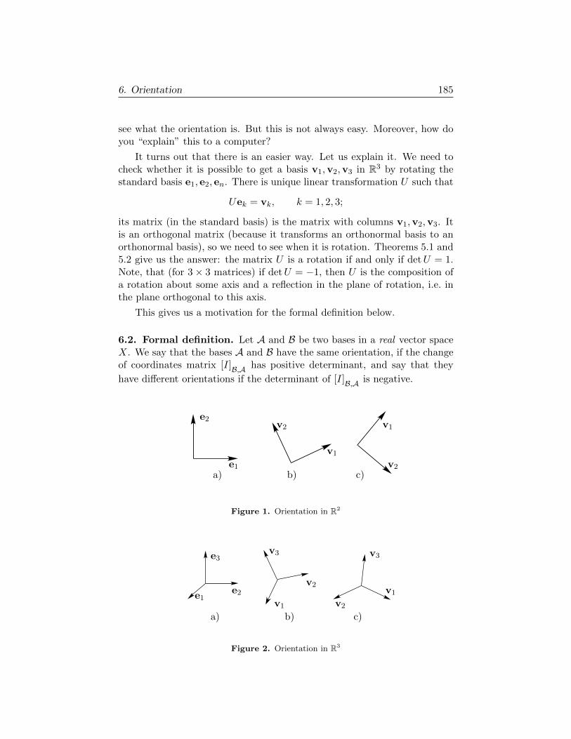
6. Orientation 185

see what the orientation is. But this is not always easy. Moreover, how doyou “explain” this to a computer?

It turns out that there is an easier way. Let us explain it. We need tocheck whether it is possible to get a basis v1,v2,v3 in R3 by rotating thestandard basis e1, e2, en. There is unique linear transformation U such that

Uek = vk, k = 1, 2, 3;

its matrix (in the standard basis) is the matrix with columns v1,v2,v3. Itis an orthogonal matrix (because it transforms an orthonormal basis to anorthonormal basis), so we need to see when it is rotation. Theorems 5.1 and5.2 give us the answer: the matrix U is a rotation if and only if detU = 1.Note, that (for 3× 3 matrices) if detU = −1, then U is the composition ofa rotation about some axis and a reflection in the plane of rotation, i.e. inthe plane orthogonal to this axis.

This gives us a motivation for the formal definition below.

6.2. Formal definition. Let A and B be two bases in a real vector spaceX. We say that the bases A and B have the same orientation, if the changeof coordinates matrix [I]B,A has positive determinant, and say that they

have different orientations if the determinant of [I]B,A is negative.

e1

e2

v1

v2 v1

v2a) b) c)

Figure 1. Orientation in R2

e1

e3

e2v1

v2

v3

v1

v2

v3

a) b) c)

Figure 2. Orientation in R3

186 6. Structure of operators in inner product spaces.

Note, that since [I]A,B = [I]−1B,A , one can use the matrix [I]A,B in the

definition.

We usually assume that the standard basis e1, e2, . . . , en in Rn has pos-itive orientation. In an abstract space one just needs to fix a basis anddeclare that its orientation is positive.

If an orthonormal basis v1,v2, . . . ,vn in Rn has positive orientation(i.e. the same orientation as the standard basis) Theorems 5.1 and 5.2 saythat the basis v1,v2, . . . ,vn is obtained from the standard basis by a rota-tion.

6.3. Continuous transformations of bases and orientation.

Definition. We say that a basis A = {a1,a2, . . . ,an} can be continuouslytransformed to a basis B = {b1,b2, . . . ,bn} if there exists a continuousfamily of bases V(t) = {v1(t),v2(t), . . . ,vn(t)}, t ∈ [a, b] such that

vk(a) = ak, vk(b) = bk, k = 1, 2 . . . , n.

“Continuous family of bases” mean that the vector-functions vk(t) are con-tinuous (their coordinates in some bases are continuous functions) and,which is essential, the system v1(t),v2(t), . . . ,vn(t) is a basis for all t ∈ [a, b].

Note, that performing a change of variables, we can always assume, ifnecessary that [a, b] = [0, 1].

Theorem 6.1. Two bases A = {a1,a2, . . . ,an} and B = {b1,b2, . . . ,bn}have the same orientation, if and only if one of the bases can be continuouslytransformed to the other.

Proof. Suppose the basis A can be continuously transformed to the basisB, and let V(t), t ∈ [a, b] be a continuous family of bases, performing thistransformation. Consider a matrix-function V (t) whose columns are thecoordinate vectors [vk(t)]A of vk(t) in the basis A.

Clearly, the entries of V (t) are continuous functions and V (a) = I,V (b) = [I]A,B. Note, that because V(t) is always a basis, detV (t) is neverzero. Then, the Intermediate Value Theorem asserts that detV (a) anddetV (b) has the same sign. Since detV (a) = det I = 1, we can concludethat

det[I]A,B = detV (b) > 0,

so the bases A and B have the same orientation.

To prove the opposite implication, i.e. the “only if” part of the theorem,one needs to show that the identity matrix I can be continuously trans-formed through invertible matrices to any matrix B satisfying detB > 0.In other words, that there exists a continuous matrix-function V (t) on an

6. Orientation 187

interval [a, b] such that for all t ∈ [a, b] the matrix V (t) is invertible and suchthat

V (a) = I, V (b) = B.

We leave the proof of this fact as an exercise for the reader. There are severalways to prove that, on of which is outlined in Problems 6.2—6.5 below. �

Exercises.

6.1. Let Rα be the rotation through α, so its matrix in the standard basis is(cosα − sinαsinα cosα

).

Find the matrix of Rα in the basis v1,v2, where v1 = e2, v2 = e1.

6.2. Let Rα be the rotation matrix

Rα =

(cosα − sinαsinα cosα

).

Show that the 2 × 2 identity matrix I2 can be continuously transformed throughinvertible matrices into Rα.

6.3. Let U be an n×n orthogonal matrix, and let detU > 0. Show that the n×nidentity matrix In can be continuously transformed through invertible matrices intoU . Hint: Use the previous problem and representation of a rotation in Rn as aproduct of planar rotations, see Section 5.

6.4. Let A be an n×n positive definite Hermitian matrix, A = A∗ > 0. Show thatthe n × n identity matrix In can be continuously transformed through invertiblematrices into A. Hint: What about diagonal matrices?

6.5. Using polar decomposition and Problems 6.3, 6.4 above, complete the proofof the “only if” part of Theorem 6.3

Chapter 7

Bilinear and quadraticforms

1. Main definition

1.1. Bilinear forms on Rn. A bilinear form on Rn is a function L =L(x,y) of two arguments x,y ∈ Rn which is linear in each argument, i.e. suchthat

1. L(αx1 + βx2,y) = αL(x1,y) + βL(x2,y);

2. L(x, αy1 + βy2) = αL(x,y1) + βL(x,y2).

One can consider bilinear form whose values belong to an arbitrary vectorspace, but in this book we only consider forms that take real values.

If x = (x1, x2, . . . , xn)T and y = (y1, y2, . . . , yn)T , a bilinear form can bewritten as

L(x,y) =n∑

j,k=1

aj,kxkyj ,

or in matrix form

L(x,y) = (Ax,y)

where

A =

a1,1 a1,2 . . . a1,n

a2,1 a2,2 . . . a2,n...

.... . .

...an,1 an,2 . . . an,n

.

The matrix A is determined uniquely by the bilinear form L.

189

190 7. Bilinear and quadratic forms

1.2. Quadratic forms on Rn. There are several equivalent definition ofa quadratic form.

One can say that a quadratic form on Rn is the “diagonal” of a bilinearform L, i.e. that any quadratic form Q is defined by Q[x] = L(x,x) =(Ax,x).

Another, more algebraic way, is to say that a quadratic form is a homo-geneous polynomial of degree 2, i.e. that Q[x] is a polynomial of n variablesx1, x2, . . . , xn having only terms of degree 2. That means that only termsax2

k and cxjxk are allowed.

There many ways (in fact, infinitely many) to write a quadratic formQ[x] as Q[x] = (Ax,x). For example, the quadratic form Q[x] = x2

1 +x2

2 − 4x1x2 on R2 can be represented as (Ax,x) where A can be any of thematrices (

1 −40 1

),

(1 0−4 1

),

(1 −2−2 1

).

In fact, any matrix A of form(1 a− 4−a 1

)will work.

But if we require the matrix A to be symmetric, then such a matrix isunique:

Any quadratic form Q[x] on Rn admits unique representationQ[x] = (Ax,x) where A is a (real) symmetric matrix.

For example, for the quadratic form

Q[x] = x21 + 3x2

2 + 5x23 + 4x1x2 − 16x1x3 + 7x2x3

on R3, the corresponding symmetric matrix A is 1 2 −82 3 3.5−8 3.5 5

.

1.3. Quadratic forms on Cn. One can also define a quadratic form on Cn(or any complex inner product space) by taking a self-adjoint transformationA = A∗ and defining Q by Q[x] = (Ax,x). While our main examples willbe in Rn, all the theorems are true in the setting of Cn as well. Bearing thisin mind, we will always use A∗ instead of AT

The only essential difference with the real case is that in the complexcase we do not have any freedom of choice: if the quadratic form is real, thecorresponding matrix has to be Hermitian (self-adjoint).

2. Diagonalization of quadratic forms 191

Note that if A = A∗ then

(Ax,x) = (x, A∗x) = (x, Ax) = (Ax,x),

so (Ax,x) ∈ R.

The converse is also true.

Lemma 1.1. Let (Ax,x) is real for all x ∈ Cn. Then A = A∗.

We leave the proof as an exercise for the reader, see Problem 1.4 below

Exercises.

1.1. Find the matrix of the bilinear form L on R3,

L(x,y) = x1y1 + 2x1y2 + 14x1y3− 5x2y1 + 2x2y2− 3x2y3 + 8x3y1 + 19x3y2− 2x3y3.

1.2. Define the bilinear form L on R2 by

L(x,y) = det[x,y],

i.e. to compute L(x,y) we form a 2× 2 matrix with columns x,y and compute itsdeterminant.

Find the matrix of L.

1.3. Find the matrix of the quadratic form Q on R3

Q[x] = x21 + 2x1x2 − 3x1x3 − 9x2

2 + 6x2x3 + 13x23.

1.4. Prove Lemma 1.1 above.

Hint: Consider the expression (A(x + zy),x + zy) and show that if it is real

for all z ∈ C then (Ax,y) = (y, A∗x)

2. Diagonalization of quadratic forms

You have probably met quadratic forms before, when you studied secondorder curves in the plane. Maybe you even studied the second order surfacesin R3.

We want to present a unified approach to classification of such objects.Suppose we are given a set in Rn defined by the equation Q[x] = 1, whereQ is some quadratic form. If Q has some simple form, for example if thecorresponding matrix is diagonal, i.e. if Q[x] = a1x

21 + a2x

22 + . . .+ anx

2n, we

can easily visualize this set, especially if n = 2, 3. In higher dimensions, itis also possible, if not to visualize, then to understand the structure of theset very well.

So, if we are given a general, complicated quadratic form, we want tosimplify it as much as possible, for example to make it diagonal. The stan-dard way of doing that is the change of variables.

192 7. Bilinear and quadratic forms

2.1. Orthogonal diagonalization. Let us have a quadratic form Q[x] =(Ax,x) in Rn. Introduce new variables y = (y1, y2, . . . , yn)T ∈ Rn, withy = S−1x, where S is some invertible n× n matrix, so x = Sy.

Then,

Q[x] = Q[Sy] = (ASy, Sy) = (S∗ASy,y),

so in the new variables y the quadratic form has matrix S∗AS.

So, we want to find an invertible matrix S such that the matrix S∗AS isdiagonal. Note, that it is different from the diagonalization of matrices wehad before: we tried to represent a matrix A as A = SDS−1, so the matrixD = S−1AS was diagonal. However, for orthogonal matrices U , we haveU∗ = U−1, and we can orthogonally diagonalize symmetric matrices. So wecan apply the orthogonal diagonalization we studied before to the quadraticforms.

Namely, we can represent the matrix A as A = UDU∗ = UDU−1.Recall, that D is a diagonal matrix with eigenvalues of A on the diagonal,and U is the matrix of eigenvectors (we need to pick an orthogonal basis ofeigenvectors). Then D = U∗AU , so in the variables y = U−1x the quadraticform has diagonal matrix.

Let us analyze the geometric meaning of the orthogonal diagonalization.The columns u1,u2, . . . ,un of the orthogonal matrix U form an orthonor-mal basis in Rn, let us call this basis B. The change of coordinate matrix[I]S,B from this basis to the standard one is exactly U . We know that

y = (y1, y2, . . . , yn)T = U−1x, so the coordinates y1, y2, . . . , yn can be inter-preted as coordinates of the vector x in the new basis u1,u2, . . . ,un.

So, orthogonal diagonalization allows us to visualize very well the setQ[x] = 1, or a similar one, as long as we can visualize it for diagonal matrices.

Example. Consider the quadratic form of two variables (i.e. quadratic formon R2), Q(x, y) = 2x2 +2y2 +2xy. Let us describe the set of points (x, y)T ∈R2 satisfying Q(x, y) = 1.

The matrix A of Q is

A =

(2 11 2

).

Orthogonally diagonalizing this matrix we can represent it as

A = U

(3 00 1

)U∗, where U =

1√2

(1 −11 1

),

or, equivalently

U∗AU =

(3 00 1

)=: D.

2. Diagonalization of quadratic forms 193

The set {y : (Dy,y) = 1} is the ellipse with half-axes 1/√

3 and 1. There-fore the set {x ∈ R2 : (Ax,x) = 1}, is the same ellipse only in the basis( 1√

2, 1√

2)T , (− 1√

2, 1√

2)T , or, equivalently, the same ellipse, rotated π/4.

2.2. Non-orthogonal diagonalization. Orthogonal diagonalization in-volves computing eigenvalues and eigenvectors, so it may be difficult to dowithout computers for n > 2. There is another way of diagonalization basedon completion of squares, which is easier to do without computers.

Let us again consider the quadratic form of two variables, Q[x] = 2x21 +

2x1x2 + 2x22 (it is the same quadratic form as in the above example, only

here we call variables not x, y but x1, x2). Since

2

(x1 +

1

2x2

)2

= 2

(x2

1 + 2x11

2x2 +

1

4x2

2

)= 2x2

1 + 2x1x2 +1

2x2

2

(note, that the first two terms coincide with the first two terms of Q), weget

2x21 + 2x1x2 + 2x2

2 = 2

(x1 +

1

2x2

)2

+3

2x2

2 = 2y21 +

3

2y2

2,

where y1 = x1 + 12x2 and y2 = x2.

The same method can be applied to quadratic form of more than 2variables. Let us consider, for example, a form Q[x] in R3,

Q[x] = x21 − 6x1x2 + 4x1x3 − 6x2x3 + 8x2

2 − 3x23.

Considering all terms involving the first variable x1 (the first 3 terms in thiscase), let us pick a full square or a multiple of a full square which has exactlythese terms (plus some other terms).

Since

(x1 − 3x2 + 2x3)2 = x21 − 6x1x2 + 4x1x3 − 12x2x3 + 9x2

2 + 4x23

we can rewrite the quadratic form as

(x1 − 3x2 + 2x3)2 − x22 + 6x2x3 − 7x2

3.

Note, that the expression −x22 + 6x2x3 − 7x2

3 involves only variables x2 andx3. Since

−(x2 − 3x3)2 = −(x22 − 6x2x3 + 9x2

3) = −x22 + 6x2x3 − 9x2

3

we have

−x22 + 6x2x3 − 7x2

3 = −(x2 − 3x3)2 + 2x23.

Thus we can write the quadratic form Q as

Q[x] = (x1 − 3x2 + 2x3)2 − (x2 − 3x3)2 + 2x23 = y2

1 − y22 + 2y2

3

where

y1 = x1 − 3x2 + 2x3, y2 = x2 − 3x3, y3 = x3.

194 7. Bilinear and quadratic forms

There is another way of performing non-orthogonal diagonalization of aquadratic form. The idea is to perform row operations on the matrix A ofthe quadratic form. The difference with the row reduction (Gauss–Jordanelimination) is that after each row operation we need to perform the samecolumn operation, the reason for that being that we want to make the matrixS∗AS diagonal.

Let us explain how everything works on an example. Suppose we wantto diagonalize a quadratic form with matrix

A =

1 −1 3−1 2 1

3 1 1

.

We augment the matrix A by the identity matrix, and perform on the aug-mented matrix (A|I) row/column operations. After each row operation wehave to perform on the matrix A the same column operation. We get 1 −1 3 1 0 0

−1 2 1 0 1 03 1 1 0 0 1

+R1 ∼

1 −1 3 1 0 00 1 4 1 1 03 1 1 0 0 1

∼ 1 0 3 1 0 0

0 1 4 1 1 03 4 1 0 0 1

−3R1

∼

1 0 3 1 0 00 1 4 1 1 00 4 −8 −3 0 1

∼ 1 0 0 1 0 0

0 1 4 1 1 00 4 −8 −3 0 1

−4R2

∼

1 0 0 1 0 00 1 4 1 1 00 0 −24 −7 −4 1

∼ 1 0 0 1 0 0

0 1 0 1 1 00 0 −24 −7 −4 1

.

Note, that we perform column operations only on the left side of the aug-mented matrix

We get the diagonal D matrix on the left, and the matrix S∗ on theright, so D = S∗AS, 1 0 0

0 1 00 0 −24

=

1 0 01 1 0−7 −4 1

1 −1 3−1 2 1

3 1 1

1 1 −70 1 −40 0 1

.

Let us explain why the method works. A row operation is a left multipli-cation by an elementary matrix. The corresponding column operation isthe right multiplication by the transposed elementary matrix. Therefore,performing row operations E1, E2, . . . , EN and the same column operationswe transform the matrix A to

(2.1) EN . . . E2E1AE∗1E∗2 . . . E

∗N = EAE∗.

2. Diagonalization of quadratic forms 195

As for the identity matrix in the right side, we performed only row operationson it, so the identity matrix is transformed to

EN . . . E2E1I = EI = E.

If we now denote E∗ = S we get that S∗AS is a diagonal matrix, and thematrix E = S∗ is the right half of the transformed augmented matrix.

In the above example we got lucky, because we did not need to inter-change two rows. This operation is a bit tricker to perform. It is quitesimple if you know what to do, but it may be hard to guess the correct rowoperations. Let us consider, for example, a quadratic form with the matrix

A =

(0 11 0

)If we want to diagonalize it by row and column operations, the simplestidea would be to interchange rows 1 and 2. But we also must to performthe same column operation, i.e. interchange columns 1 and 2, so we will endup with the same matrix.

So, we need something more non-trivial. The identity

2x1x2 =1

2

[(x1 + x2)2 − (x1 − x2)2

]gives us the idea for the following series of row operations:(

0 1 1 01 0 0 1

)−1

2R1∼(

0 1 1 01 −1/2 −1/2 1

)∼(

0 1 1 01 −1 −1/2 1

)+R1 ∼

(1 0 1/2 11 −1 −1/2 1

)∼(

1 0 1/2 10 −1 −1/2 1

).

Non-orthogonal diagonalization gives us a simple description of a setQ[x] = 1 in a non-orthogonal basis. It is harder to visualize, then the rep-resentation given by the orthogonal diagonalization. However, if we are notinterested in the details, for example if it is sufficient for us to know that theset is ellipsoid (or hyperboloid, etc), then the non-orthogonal diagonalizationis an easier way to get the answer.

Remark. For quadratic forms with complex entries, the non-orthogonal di-agonalization works the same way as in the real case, with the only difference,that the corresponding “column operations” have the complex conjugate co-efficient.

The reason for that is that if a row operation is given by left multiplica-tion by an elementary matrix Ek, then the corresponding column operationis given by the right multiplication by E∗k , see (2.1).

196 7. Bilinear and quadratic forms

Note that formula (2.1) works in both complex and reals cases: in realcase we could write ETk instead of E∗k , but using Hermitian adjoint allowsus to have the same formula in both cases.

Exercises.

2.1. Diagonalize the quadratic form with the matrix

A =

1 2 12 3 21 2 1

.

Use two methods: completion of squares and row operations. Which one do youlike better?

Can you say if the matrix A is positive definite or not?

2.2. For the matrix A

A =

2 1 11 2 11 1 2

orthogonally diagonalize the corresponding quadratic form, i.e. find a diagonal ma-trix D and a unitary matrix U such that D = U∗AU .

3. Silvester’s Law of Inertia

As we discussed above, there are many ways to diagonalize a quadratic form.Note, that a resulting diagonal matrix is not unique. For example, if we gota diagonal matrix

D = diag{λ1, λ2, . . . , λn},we can take a diagonal matrix

S = diag{s1, s2, . . . , sn}, sk ∈ R, sk 6= 0

and transform D to

S∗DS = diag{s21λ1, s

22λ2, . . . , s

2nλn}.

This transformation changes the diagonal entries of D. However, it does notchange the signs of the diagonal entries. And this is always the case!

Namely, the famous Silvester’s Law of Inertia states that:

For a Hermitian matrix A (i.e. for a quadratic form Q[x] =(Ax,x)) and any of its diagonalization D = S∗AS, the numberof positive (negative, zero) diagonal entries of D depends only onA, but not on a particular choice of diagonalization.

Here we of course assume that S is an invertible matrix, and D is a diagonalone.

3. Silvester’s Law of Inertia 197

The idea of the proof of the Silvester’s Law of Inertia is to express thenumber of positive (negative, zero) diagonal entries of a diagonalizationD = S∗AS in terms of A, not involving S or D.

We will need the following definition.

Definition. Given an n × n symmetric matrix A = A∗ (a quadratic formQ[x] = (Ax,x) on Rn) we call a subspace E ⊂ Rn positive (resp. negative,resp. neutral) if

(Ax,x) > 0 (resp. (Ax,x) < 0, resp. (Ax,x) = 0)

for all x ∈ E, x 6= 0.

Sometimes, to emphasize the role of A we will say A-positive (A negative,A-neutral).

Theorem 3.1. Let A be an n× n symmetric matrix, and let D = S∗AS beits diagonalization by an invertible matrix S. Then the number of positive(resp. negative) diagonal entries of D coincides with the maximal dimensionof an A-positive (resp. A-negative) subspace.

The above theorem says that if r+ is the number of positive diagonalentries of D, then there exists an A-positive subspace E of dimension r+,but it is impossible to find a positive subspace E with dimE > r+.

We will need the following lemma, which can be considered a particularcase of the above theorem.

Lemma 3.2. Let D be a diagonal matrix D = diag{λ1, λ2, . . . , λn}. Thenthe number of positive (resp. negative) diagonal entries of D coincides withthe maximal dimension of a D-positive (resp. D-negative) subspace.

Proof. By rearranging the standard basis in Rn (changing the numeration)we can always assume without loss of generality that the positive diagonalentries of D are the first r+ diagonal entries.

Consider the subspace E+ spanned by the first r+ coordinate vectorse1, e2, . . . , er+ . Clearly E+ is a D-positive subspace, and dimE+ = r+.

Let us now show that for any other D-positive subspace E we havedimE ≤ r+. Consider the orthogonal projection P = P

E+,

Px = (x1, x2, . . . , xr+ , 0 . . . , 0)T , x = (x1, x2, . . . , xn)T .

For a D-positive subspace E define an operator T : E → E+ by

Tx = Px, ∀x ∈ E.In other words, T is the restriction of the projection P : P is defined onthe whole space, but we restricted its domain to E and target space to E+.

198 7. Bilinear and quadratic forms

We got an operator acting from E to E+, and we use a different letter todistinguish it from P .

Note, that KerT = {0}. Indeed, let for x = (x1, x2, . . . , xn)T ∈ E wehave Tx = Px = 0. Then, by the definition of P

x1 = x2 = . . . = xr+ = 0,

and therefore

(Dx,x) =n∑

k=r++1

λkx2k ≤ 0 (λk ≤ 0 for k > r+).

But x belongs to a D-positive subspace E, so the inequality (Dx,x) ≤ 0holds only for x = 0.

Let us now apply the Rank Theorem (Theorem 7.1 from Chapter 2).First of all, rankT = dim RanT ≤ dimE+ = r+ because RanT ⊂ E+. Bythe Rank Theorem, dim KerT + rankT = dimE. But we just proved thatKerT = {0}, i.e. that dim KerT = 0, so

dimE = rankT ≤ dimE+ = r+.

To prove the statement about negative entries, we just apply the abovereasoning to the matrix −D. �

Proof of Theorem 3.1. Let D = S∗AS be a diagonalization of A. Since

(Dx,x) = (S∗ASx,x) = (ASx, Sx)

it follows that for any D-positive subspace E, the subspace SE is an A-positive subspace. The same identity implies that for any A-positive sub-space F the subspace S−1F is D-positive.

Since S and S−1 are invertible transformations, dimE = dimSE anddimF = dimS−1F . Therefore, for any D positive subspace E we can findan A-positive subspace (namely SE) of the same dimension, and vice versa:for any A-positive subspace F we can find a D-positive subspace (namelyS−1F ) of the same dimension. Therefore the maximal possible dimensions ofa A-positive and a D-positive subspace coincide, and the theorem is proved.

The case of negative diagonal entries treated similarly, we leave thedetails as an exercise to the reader. �

4. Positive definite forms. Minimax characterization ofeigenvalues and the Silvester’s criterion of positivity

Definition. A quadratic form Q is called

• Positive definite if Q[x] > 0 for all x 6= 0.

• Positive semidefinite if Q[x] ≥ 0 for all x.

4. Positive definite forms. Minimax. Silvester’s criterion 199

• Negative definite if Q[x] < 0 for all x 6= 0.

• Negative semidefinite if Q[x] ≤ 0 for all x.

• Indefinite if it take both positive and negative values, i.e. if thereexist vectors x1 and x2 such that Q[x1] > 0 and Q[x2] < 0.

Definition. A symmetric matrix A = A∗ is called positive definite (negativedefinite, etc. . . ) if the corresponding quadratic form Q[x] = (Ax,x) ispositive definite (negative definite, etc. . . ).

Theorem 4.1. Let A = A∗. Then

1. A is positive definite iff all eigenvalues of A are positive.

2. A is positive semidefinite iff all eigenvalues of A are non-negative.

3. A is negative definite iff all eigenvalues of A are negative.

4. A is negative semidefinite iff all eigenvalues of A are non-positive.

5. A is indefinite iff it has both positive and negative eigenvalues.

Proof. The proof follows trivially from the orthogonal diagonalization. In-deed, there is an orthonormal basis in which matrix of A is diagonal, andfor diagonal matrices the theorem is trivial. �

Remark. Note, that to find whether a matrix (a quadratic form) is positivedefinite (negative definite, etc) one does not have to compute eigenvalues.By Silvester’s Law of Inertia it is sufficient to perform an arbitrary, notnecessarily orthogonal diagonalization D = S∗AS and look at the diagonalentries of D.

4.1. Silvester’s criterion of positivity. It is an easy exercise to see thata 2× 2 matrix

A =

(a bb c

)is positive definite if and only if

(4.1) a > 0 and detA = ac− b2 > 0

Indeed, if a > 0 and detA = ac− b2 > 0, then c > 0, so traceA = a+ c > 0.So we know that if λ1, λ2 are eigenvalues of A then λ1λ2 > 0 (detA > 0)and λ1 + λ2 = traceA > 0. But that only possible if both eigenvalues arepositive. So we have proved that conditions (4.1) imply that A is positivedefinite. The opposite implication is quite simple, we leave it as an exercisefor the reader.

200 7. Bilinear and quadratic forms

This result can be generalized to the case of n×n matrices. Namely, fora matrix A

A =

a1,1 a1,2 . . . a1,n

a2,1 a2,2 . . . a2,n...

.... . .

...an,1 an,2 . . . an,n

let us consider its all upper left submatrices

A1 = (a1,1), A2 =

(a1,1 a1,2

a2,1 a2,2

), A3 =

a1,1 a1,2 a1,3

a2,1 a2,2 a2,3

a3,1 a3,2 a3,3

, . . . , An = A

Theorem 4.2 (Silvester’s Criterion of Positivity). A matrix A = A∗ ispositive definite if and only if

detAk > 0 for all k = 1, 2, . . . , n.

First of all let us notice that if A > 0 then Ak > 0 also (can you explainwhy?). Therefore, since all eigenvalues of a positive definite matrix arepositive, see Theorem 4.1, detAk > 0 for all k.

One can show that if detAk > 0 ∀k then all eigenvalues of A are posi-tive by analyzing diagonalization of a quadratic form using row and columnoperations, which was described in Section 2.2. The key here is the obser-vation that if we perform row/column operations in natural order (i.e. firstsubtracting the first row/column from all other rows/columns, then sub-tracting the second row/columns from the rows/columns 3, 4, . . . , n, and soon. . . ), and if we are not doing any row interchanges, then we automaticallydiagonalize quadratic forms Ak as well. Namely, after we subtract first andsecond rows and columns, we get diagonalization of A2; after we subtractthe third row/column we get the diagonalization of A2, and so on.

Since we are performing only row replacement we do not change thedeterminant. Moreover, since we are not performing row exchanges andperforming the operations in the correct order, we preserve determinants ofAk. Therefore, the condition detAk > 0 guarantees that each new entry inthe diagonal is positive.

Of course, one has to be sure that we can use only row replacements, andperform the operations in the correct order, i.e. that we do not encounterany pathological situation. If one analyzes the algorithm, one can see thatthe only bad situation that can happen is the situation where at some stepwe have zero in the pivot place. In other words, if after we subtracted thefirst k rows and columns and obtained a diagonalization of Ak, the entry inthe k + 1st row and k + 1st column is 0. We leave it as an exercise for thereader to show that this is impossible. �

4. Positive definite forms. Minimax. Silvester’s criterion 201

The proof we outlined above is quite simple. However, let us present, inmore detail, another one, which can be found in more advanced textbooks.I personally prefer this second proof, for it demonstrates some importantconnections.

We will need the following characterization of eigenvalues of a hermitianmatrix.

4.2. Minimax characterization of eigenvalues. Let us recall that thecodimension of a subspace E ⊂ X is by the definition the dimension of itsorthogonal complement, codimE = dim(E⊥). Since for a subspace E ⊂ X,dimX = n we have dimE + dimE⊥ = n, we can see that codimE =dimX − dimE.

Recall that the trivial subspace {0} has dimension zero, so the wholespace X has codimension 0.

Theorem 4.3 (Minimax characterization of eigenvalues). Let A = A∗ bean n× n matrix, and let λ1 ≥ λ2 ≥ . . . ≥ λn be its eigenvalues taken in thedecreasing order. Then

λk = maxE:

dimE=k

minx∈E‖x‖=1

(Ax,x) = minF :

codimF=k−1

maxx∈F‖x‖=1

(Ax,x).

Let us explain in more details what the expressions like max min andmin max mean. To compute the first one, we need to consider all subspacesE of dimension k. For each such subspace E we consider the set of all x ∈ Eof norm 1, and find the minimum of (Ax,x) over all such x. Thus for eachsubspace we obtain a number, and we need to pick a subspace E such thatthe number is maximal. That is the max min.

The min max is defined similarly.

Remark. A sophisticated reader may notice a problem here: why do themaxima and minima exist? It is well known, that maximum and minimumhave a nasty habit of not existing: for example, the function f(x) = x hasneither maximum nor minimum on the open interval (0, 1).

However, in this case maximum and minimum do exist. There are twopossible explanations of the fact that (Ax,x) attains maximum and mini-mum. The first one requires some familiarity with basic notions of analysis:one should just say that the unit sphere in E, i.e. the set {x ∈ E : ‖x‖ = 1}is compact, and that a continuous function (Q[x] = (Ax,x) in our case) ona compact set attains its maximum and minimum.

Another explanation will be to notice that the function Q[x] = (Ax,x),x ∈ E is a quadratic form on E. It is not difficult to compute the matrixof this form in some orthonormal basis in E, but let us only note that thismatrix is not A: it has to be a k × k matrix, where k = dimE.

202 7. Bilinear and quadratic forms

It is easy to see that for a quadratic form the maximum and minimumover a unit sphere is the maximal and minimal eigenvalues of its matrix.

As for optimizing over all subspaces, we will prove below that the max-imum and minimum do exist.

Proof of Theorem 4.3. First of all, by picking an appropriate orthonor-mal basis, we can assume without loss of generality that the matrix A isdiagonal, A = diag{λ1, λ2, . . . , λn}.

Pick subspaces E and F , dimE = k, codimF = k − 1, i.e. dimE =n−k+1. Since dimE+dimF > n, there exists a non-zero vector x0 ∈ E∩F .By normalizing it we can assume without loss of generality that ‖x0‖ = 1.We can always arrange the eigenvalues in decreasing order, so let us assumethat λ1 ≥ λ2 ≥ . . . ≥ λn.

Since x belongs to the both subspaces E and F

minx∈E‖x‖=1

(Ax,x) ≤ (Ax0,x0) ≤ maxx∈F‖x‖=1

(Ax,x).

We did not assume anything except dimensions about the subspaces E andF , so the above inequality

(4.2) minx∈E‖x‖=1

(Ax,x) ≤ maxx∈F‖x‖=1

(Ax,x).

holds for all pairs of E and F of appropriate dimensions.

Define

E0 := span{e1, e2, . . . , ek}, F0 := span{ek, ek+1, ek+2, . . . , en}.Since for a self-adjoint matrix B, the maximum and minimum of (Bx,x) overthe unit sphere {x : ‖x‖ = 1} are the maximal and the minimal eigenvaluerespectively (easy to check on diagonal matrices), we get that

minx∈E0‖x‖=1

(Ax,x) = maxx∈F0‖x‖=1

(Ax,x) = λk.

It follows from (4.2) that for any subspace E, dimE = k

minx∈E‖x‖=1

(Ax,x) ≤ maxx∈F0‖x‖=1

(Ax,x) = λk

and similarly, for any subspace F of codimension k − 1,

maxx∈F‖x‖=1

(Ax,x) ≥ minx∈E0‖x‖=1

(Ax,x) = λk.

But on subspaces E0 and F0 both maximum and minimum are λk, somin max = max min = λk. �

4. Positive definite forms. Minimax. Silvester’s criterion 203

Corollary 4.4 (Intertwining of eigenvalues). Let A = A∗ = {aj,k}nj,k=1

be a self-adjoint matrix, and let A = {aj,k}n−1j,k=1 be its submatrix of size

(n− 1)× (n− 1). Let λ1, λ2, . . . , λn and µ1, µ2, . . . , µn−1 be the eigenvalues

of A and A respectively, taken in decreasing order. Then

λ1 ≥ µ1 ≥ λ2 ≥ µ2 ≥ . . . ≥ λn−1 ≥ µn−1 ≥ λn.i.e.

λk ≥ µk ≥ λk+1, k = 1, 2, . . . , n− 1

Proof. Let X ⊂ Fn be the subspace spanned by the first n−1 basis vectors,

X = span{e1, e2, . . . , en−1}. Since (Ax,x) = (Ax,x) for all x ∈ X, Theorem4.3 implies that

µk = maxE⊂X

dimE=k

minx∈E‖x‖=1

(Ax,x).

To get λk we need to get maximum over the set of all subspaces E of Fn,

dimE = k, i.e. take maximum over a bigger set (any subspace of X is asubspace of Fn). Therefore

µk ≤ λk.(the maximum can only increase, if we increase the set).

On the other hand, any subspace E ⊂ X of codimension k − 1 (here

we mean codimension in X) has dimension n − 1 − (k − 1) = n − k, so itscodimension in Fn is k. Therefore

µk = minE⊂X

dimE=n−k

maxx∈E‖x‖=1

(Ax,x) ≤ minE⊂Fn

dimE=n−kmaxx∈E‖x‖=1

(Ax,x) = λk+1

(minimum over a bigger set can only be smaller). �

Proof of Theorem 4.2. If A > 0, then Ak > 0 for k = 1, 2, . . . , n as well(can you explain why?). Since all eigenvalues of a positive definite matrixare positive (see Theorem 4.1), detAk > 0 for all k = 1, 2, . . . , n.

Let us now prove the other implication. Let detAk > 0 for all k. Wewill show, using induction in k, that all Ak (and so A = An) are positivedefinite.

Clearly A1 is positive definite (it is 1 × 1 matrix, so A1 = detA1).Assuming that Ak−1 > 0 (and detAk > 0) let us show that Ak is positivedefinite. Let λ1, λ2, . . . , λk and µ1, µ2, . . . , µk−1 be eigenvalues of Ak andAk−1 respectively. By Corollary 4.4

λj ≥ µj > 0 for j = 1, 2, . . . , k − 1.

Since detAk = λ1λ2 . . . λk−1λk > 0, the last eigenvalue λk must also bepositive. Therefore, since all its eigenvalues are positive, the matrix Ak ispositive definite. �

204 7. Bilinear and quadratic forms

Exercises.

4.1. Using Silvester’s Criterion of Positivity check if the matrices

A =

4 2 12 3 −11 −1 2

, B =

3 −1 2−1 4 −2

2 −2 1

are positive definite or not.

Are the matrices −A, A3 and A−1, A+B−1, A+B, A−B positive definite?

4.2. True or false:

a) If A is positive definite, then A5 is positive definite.

b) If A is negative definite, then A8 is negative definite.

c) If A is negative definite, then A12 is positive definite.

d) If A is positive definite and B is negative semidefinite, then A−B is positivedefinite.

e) If A is indefinite, and B is positive definite, then A+B is indefinite.

5. Positive definite forms and inner products

Let V be an inner product space and let B = v1,v2, . . . ,vn be a basis (notnecessarily orthogonal) in V . Let A = {aj,k}nj.k=1 be the matrix defined by

aj,k = (vk,vj).

If x =∑

k xkvk and y =∑

k ykvk, then

(x,y) =

∑k

xkvk,∑j

yjvj

=n∑

k,j=1

xkyj(vk,vj)

=

n∑j=1

n∑k=1

aj,kxkyj = (A[x]B, [y]B)Cn ,

where ( · , · )Cn stands for the standard inner product in Cn. One can im-mediately see that A is a positive definite matrix (why?).

So, when one works with coordinates in an arbitrary (not necessarilyorthogonal) basis in an inner product space, the inner product (in terms ofcoordinates) is not computed as the standard inner product in Cn, but withthe help of a positive definite matrix A as described above.

Note, that this A-inner product coincides with the standard inner prod-uct in Cn if and only if A = I, which happens if and only if the basisv1,v2, . . . ,vn is orthonormal.

Conversely, given a positive definite matrix A one can define a non-standard inner product (A-inner product) in Cn by

(x,y)A := (Ax,y)Cn , x,y ∈ Cn.

5. Positive definite forms and inner products 205

One can easily check that (x,y)A is indeed an inner product, i.e. that prop-erties 1–4 from Section 1.3 of Chapter 5 are satisfied.

Chapter 8

Dual spaces andtensors

All vector spaces in this chapter are finite-dimensional.

1. Dual spaces

1.1. Linear functionals and the dual space. Change of coordinatesin the dual space.

Definition 1.1. A linear functional on a vector space V (over a field F) isa linear transformation L : V → F.

This special class of linear transformation sufficiently important to de-serve a separate name.

If one thinks of vectors as of some physical objects, like force or velocity,then one can think of a linear functional as a (linear) measurement, thatgives you some a scalar quantity as the result: think about force or velocityin a given direction.

Definition 1.2. A collection of all linear functionals on a finite-dimensional1

vector space V is called the dual of V and is usually denoted as V ′ or V ∗

As it was discussed earlier in Section 4 of Chapter 1, the collectionL(V,W ) of all linear transformations acting from V to W is a vector space

1We consider here only finite-dimensional spaces because for infinite-dimensional spaces the

dual space consists not of all but only of the so-called bounded linear functionals. Without givingthe precise definition, let us only mention than in the finite-dimensional case (both the domainand the target space are finite-dimensional) all linear transformations are bounded, and we do notneed to mention the word bounded

207

208 8. Dual spaces and tensors

(with naturally defined operations of addition and multiplication by a scalar.So, the dual space V ′ = L(V,F) is a vector space.

Let us consider an example. Let the space V be Rn, what is its dual? Aswe know, a linear transformation T : Rn → Rm is represented by an m× nmatrix, so a linear functional on Rn (i.e. a linear transformation L : Rn → Ris given by an 1 × n matrix (row), let us denote it by [L]. The collectionof all such rows is isomorphic to Rn (isomorphism is given by taking thetranspose [L]→ [L]T ).

So, the dual of Rn is Rn itself. The same holds true for Cn, of course, aswell as for Fn, where F is an arbitrary field. Since the space V over a fieldF (here we mostly interested in the case F = R or F = C) of dimension n isisomorphic to Fn, and the dual to Fn is isomorphic to Fn, we can concludethat the dual V ′ is isomorphic to V

Thus, the definition of the dual space is starting to look a bit silly, sinceit does not appear to give us anything new.

However, that is not the case! If we look carefully, we can see that thedual space is indeed a new object. To see that, let us analyze how the entriesof the matrix [L] (which we can call the coordinates of L) change when wechange the basis in V .

1.1.1. Change of coordinates formula. Let

A = {a1,a2, . . . ,an}, B = {b1,b2, . . . ,bn}be two bases in V , and let [L]A = [L]S,A and [L]B = [L]S,B be the matrices ofL in the bases A and B respectively (we suppose that the basis in the targetspace of scalars is always the standard one, so we can skip the subscript Sin the notation). Then recalling the change of coordinate rule from Section8.4 in Chapter 2 we get that

[L]B = [L]A[I]A,B.

Recall that for a vector v ∈ V its coordinates in different bases are relatedby the formula

[v]B = [I]B,A[v]A,

and that

[I]A,B = [I]−1B,A.

If we denote S := [I]B,A, so [v]B = S[v]A, the entries of the vectors [L]TBand [L]TA are related by the formula

(1.1) [L]TB = (S−1)T [L]TA

(since we usually represent a vector as a column of its coordinates, we use[L]TA and [L]TB instead of [L]A and [L]B)

Saying it in words

1. Dual spaces 209

If S is the change of coordinate matrix (from old coordinates tothe new ones) in X, then the change of coordinate matrix in thedual space X ′ is (S−1)T .

So, the dual space V ′ of V while isomorphic to V is indeed a differentobject: the difference is in how the coordinates in V and V ′ change whenone changes the basis in V .

Remark. One can ask: why can’t we pick a basis in X and some completelyunrelated basis in the dual X ′? Of course, we can do that, but imagine, whatwould it take to compute L(x), knowing coordinates of x in some basis andcoordinates of L in some completely unrelated basis.

So, if we want (knowing the coordinates of a vector x in some basis)to compute the action of a linear functional L using the standard rules ofmatrix algebra, i.e. to multiply a row (the functional) by a column (thevector), we have no choice: the “coordinates” of the linear functional Lshould be the entries of its matrix (in the same basis).

As we can see later, see Section 1.3 below, the entries (“coordinates”)of a linear functional are indeed the coordinates in some basis (the so-calleddual basis.

1.1.2. A uniqueness theorem.

Lemma 1.3. Let v ∈ V . If L(v) = 0 for all L ∈ V ′ then v = 0. As acorollary, if L(v1) = L(v2) for all L ∈ V ′, then v1 = v2

Proof. Fix a basis B in V . Then

L(v) = [L]B[v]B.

Picking different matrices (i.e. different L) we can easily see that [v]B = 0.Indeed, if

Lk = [0, . . . , 0, 1k, 0, . . . , 0]

then the equality

Lk[v]B = 0

implies that kth coordinate of [v]B is 0.

Using this equality for all k we conclude that [v]B = 0, so v = 0. �

1.2. Second dual. As we discussed above, the dual space V ′ is a vectorspace, so one can consider its dual V ′′ = (V ′)′. It looks like one that canconsider the dual V ′′′ of V ′′ and so on. . . However, the fun stops with V ′′

because

The second dual V ′′ is canonically (i.e. in a natural way) isomor-phic to V

210 8. Dual spaces and tensors

Let us decipher this statement. Any vector v ∈ V canonically defines alinear functional Lv on V ′ (i.e. an element of the second dual V ′′ by the rule

Lv(f) = f(v) ∀f ∈ V ′

It is easy to check that the mapping T : V → V ′′, Tv = Lv is a lineartransformation.

Note, that KerT = {0}. Indeed, if Tv = 0, then

f(v) = 0 ∀f ∈ V ′,

and by Lemma 1.3 above we have v = 0.

Since dimV ′′ = dimV ′ = dimV , the condition KerT = {0} implies thatT is an invertible transformation (isomorphism).

The isomorphism T is very natural, (at least for a mathematician). Inparticular, it was defined without using a basis, so it does not depend onthe choice of basis. So, informally we say that V ′′ is canonically isomorphicto V : the rigorous statement is that the map T described above (which weconsider to be a natural and canonical) is an isomorphism from V to V ′′.

1.3. Dual, a.k.a. biorthogonal bases. In the previous sections, we sev-eral times referred to the entries of the matrix of a linear functional L ascoordinates. But coordinates in this book usually means the coordinates insome basis. Are the “coordinates’ of a linear functional really coordinatesin some basis? Turns out the answer is “yes”, so the terminology remainsconsistent.

Let us find the basis corresponding to the coordinates of L ∈ V ′. Let{b1,b2, . . . ,bn} be a basis in V . For L ∈ V ′, let [L]B = [L1, L2, . . . , Ln] beits matrix (row) in the basis B. Consider linear functionals b′1,b

′2, . . . ,b

′n ∈

V ′ defined by

(1.2) b′k(bj) = δk,j

where δk,j is the Kroneker delta,

δk.j =

{1, j = k0 j 6= k

Recall, that a linear transformation is defined by its action on a basis, sothe functionals b′k are well defined.

then (1.2) can be rewritten as b′k(bj) = δk, j.

As one can easily see, the functional L can be represented as

L =∑

Lkb′k.

1. Dual spaces 211

Indeed, take an arbitrary v =∑

k αkbk ∈ V , so [v]B = [α1, α2, . . . , αn]T .By linearity and definition of b′k

b′k(v) = b′k

∑j

αjbj

=∑j

αjv′k(bj) = αk.

ThereforeLv = [L]B[v]B =

∑k

Lkαk =∑k

Lkb′k(v).

Since this identity holds for all v ∈ V , we conclude that L =∑

k Lkb′k.

Since we did not assume anything about L ∈ V ′, we have just shownthat any linear functional L can be represented as a linear combination ofb′1,b

′2, . . . ,b

′n, so the system b′1,b

′2, . . . ,b

′n is generating.

Let us show that this system is linearly independent (and so it is a basis).Let 0 =

∑k Lkb

′k. Then for an arbitrary j = 1, 2, . . . , n

0 = 0bj =

(∑k

Lkb′k

)(bj) =

∑k

Lkb′k(bj) = Lj

so Lj = 0. Therefore, all Lk are 0 and the system is linearly independent.

So, the system b′1,b′2, . . . ,b

′n is indeed a basis in the dual space V ′ and

the entries of [L]B are coordinates of L with respect to the basis B.

Definition 1.4. Let b1,b2, . . . ,bn be a basis in V . The system of vectors

b′1,b′2, . . . ,b

′n ∈ V ′,

uniquely defined by the equation (1.2) is called the dual (or biorthogonal)basis to b1,b2, . . . ,bn.

Note that we have shown that the dual system to a basis is a basis. Notealso that in b′1,b

′2, . . . ,b

′n is the dual system to a basis b1,b2, . . . ,bn, then

b1,b2, . . . ,bn is the dual to the basis b′1,b′2, . . . ,b

′n

1.3.1. Abstract non-orthogonal Fourier decomposition. The dual system canbe used for computing the coordinates in the basis b1,b2, . . . ,bn. Letb1,b2, . . . ,bn be the biorthogonal system to b1,b2, . . . ,bn, and let v =∑

k αkbk. Then, as it was shown before

b′j(v) = bj

(∑k

αkbk

)=∑k

αkbj(bk) = αjb′j(bj) = αj ,

so αk = b′k(v). Then we can write

(1.3) v =∑k

b′k(v)bk.

In other words,

212 8. Dual spaces and tensors

The kth coordinate of a vector v in a basis B = {b1,b2, . . . ,bn}is b′k(v)}, where B′ = {b′1,b′2, . . . ,b′n} is the dual basis.

This formula is called (a baby version of) the abstract non-orthogonalFourier decomposition of v (in the basis b1,b2, . . . ,bn). The reason for thisname will be clear later in Section 2.3.

Remark 1.5. Let A = {a1,a2, . . . ,an} and B = {b1,b2, . . . ,bm} be basesin X and Y respectively, and let B′ = {b′1,b′2, . . . ,b′m} be the dual basis toB. Then the matrix [T ]B,A =: A = {ak,j}mk=1

nj=1 of the transformation T in

the bases A, B is given by

ak,j = b′k(Taj), j = 1, 2, . . . , n, k = 1, 2, . . . ,m.

1.4. Examples of dual systems. The first example we consider is a trivialone. Let V be Rn (or Cn) and let e1, e2, . . . , en be the standard basis there.The dual space will be the space of n-dimensional row vectors, which isisomorphic to Rn (or Cn in the complex case), and the standard basis thereis the dual to e1, e2, . . . , en. The standard basis in (Rn)′ (or in (Cn)′ iseT1 , e

T2 , . . . , e

Tn ) obtained from e1, e2, . . . , en by transposition.

1.4.1. Taylor formula. The next example is more interesting. Let us con-sider the space Pn of polynomials of degree at most n. As we know, thepowers {ek}nk=0, e(t) = tn form the standard basis in this space. What isthe dual to this basis?

The answer might be tricky to guess, but it is very easy to check whenyou know it. Namely, consider the linear functionals e′k ∈ (Pn)′, k =0, 1, . . . , n, acting on polynomials as follows:

e′k(p) :=1

k!

dk

dtkp(t)

∣∣t=0

=1

k!p(k)(0);

here we use the usual agreement that 0! = 1 and d0f/dt0 = f .

Since

dk

dtkjj =

{j(j − 1) . . . (j − k + 1)tj−k, k ≤ j0 k > j

we can easily see that the system {e′k}nk=0 is the dual to the system of powers{ek}nk=0.

Applying (1.3) to the above system {ek}nk=0 and its dual we get thatany polynomial p of degree at most n can be represented as

(1.4) p(t) =

n∑k=0

p(k)(0)

k!tk

This formula is well-known in Calculus as the Taylor formula for polyno-mials. More precisely, this is a particular case of the Taylor formula, the

1. Dual spaces 213

so-called Maclaurin formula. The general Taylor formula

p(t) =n∑k=0

p(k)(a)

k!(t− a)k

can be obtained from (1.4) by applying it to the polynomial p(τ − a) andthen denoting t := τ − a. It also can be obtained by considering powers(t− a)k, k = 0, 1, . . . , n and finding the dual system the same way we did itfor tk.2

1.4.2. Lagrange interpolation. Our next example deals with the so-calledLagrange interpolating formula. Let a1, a2, . . . , an+1 be distinct points (inR or C), and let Pn be the space of polynomials of degree at most n. Definefunctionals fk ∈ P′n by

fk(p) = p(ak) ∀p ∈ Pn.

What is the dual of this system of functionals? Note, that while it is nothard to show that the functionals fk are linearly independent, and so (sincedim(Pn)′ = dimPn = n+ 1) form a basis in (Pn)′, we do not need that. Wewill construct the dual system directly, and then will be able to see that thesystem f1, f2, . . . , fn+1 is indeed a basis.

Namely, let us define the polynomials pk, k = 1, 2, . . . , n+ 1 as

pk(t) =∏j:j 6=k

(t− aj)/ ∏

j:j 6=k(ak − aj)

where j in the products runs from 1 to n + 1. Clearly pk(ak) = 1 andpk(aj) = 0 if j 6= k, so indeed the system p1, p2, . . . , pn+1 is dual to thesystem f1, f2, . . . , fn+1.

There is a little detail here, since the notion of a dual system was definedonly for a basis, and we did not prove that either of the systems is one.But one can immediately see that the system p1, p2, . . . , pn+1 is linearlyindependent (can you explain why?), and since it contains n + 1 = dimPnvectors, it is a basis. Therefore, the system of functionals f1, f2, . . . , fn+1 isalso a basis in the dual space (Pn)′.

Remark. Note, that we did not just got lucky here, this is a general phe-nomenon. Namely, as Problem 1.1 below asserts, any system of vectorshaving a “‘dual” one must be linearly independent. So, constructing a dualsystem is a way of proving linear independence (and an easy one, if you cando it easily as in the above example).

2 Note, that the general Taylor formula says more than the formula for polynomials obtained

here: it says that any n times differentiable function can be approximated near the point a by itsTaylor polynomial. Moreover, if the function is n+ 1 times differentiable, it allows us to estimate

the error. The above formula for polynomials serves as a motivation and a starting point for thegeneral case

214 8. Dual spaces and tensors

Applying formula (1.3) to the above example one can see that the(unique) polynomial p, deg p ≤ n satisfying

(1.5) p(ak) = yk, k = 1, 2, . . . , n+ 1

can be reconstructed by the formula

(1.6) p(t) =n+1∑k=1

ykpk(t).

This formula is well -known in mathematics as the “Lagrange interpolationformula”.

Exercises.

1.1. Let v1,v2, . . . ,vr be a system of vectors in X such that there exists a systemv′1,v

′2, . . . ,v

′r of linear functionals such that

v′k(vj) =

{1, j = k0 j 6= k

a) Show that the system v1,v2, . . . ,vr is linearly independent.

b) Show that if the system v1,v2, . . . ,vr is not generating, then the “biorthog-onal” system v′1,v

′2, . . . ,v

′r is not unique. Hint: Probably the easiest way

to prove that is to complete the system v1,v2, . . . ,vr to a basis, see Propo-sition 5.4 from Chapter 2

1.2. Prove that given distinct points a1, a2, . . . , an+1 and values y1, y2, . . . , yn+1

(not necessarily distinct) the polynomial p, deg p ≤ n satisfying (1.5) is unique.Try to prove it using the ideas from linear algebra, and not what you know aboutpolynomials.

2. Dual of an inner product space

Let us recall that there is no inner product space over an arbitrary field,that all our inner product spaces are either real or complex.

2.1. Riesz representation theorem.

Theorem 2.1 (Riesz representation theorem). Let H be an inner productspace. Given a linear functional L on H there exists a unique vector y ∈ Hsuch that

(2.1) L(v) = (v,y) ∀v ∈ H.

Proof. Fix an orthonormal basis e1, e2, . . . , en in H, and let

[L] = [L1, L2, . . . , Ln]

be the matrix of L in this basis. Define vector y by

(2.2) y :=∑k

Lkek,

2. Dual of an inner product space 215

where Lk denotes the complex conjugate of Lk. In the case of a real spacethe conjugation does nothing and can be simply ignored.

We claim that y satisfies (2.1).

Indeed, take an arbitrary vector v =∑

k αkek. Then

[v] = [α1, α2, . . . , αn]T

andL(v) = [L][v] =

∑k

Lkαk.

On the other hand Recall that if weknow coordinates of2 vectors in an or-thonormal basis, wecan compute the in-ner product by tak-ing these coordinateand computing thestandard inner prod-uct in Cn (or Rn).

(v,y) =∑k

αkLk =∑k

αkLk

so (2.1) holds.

To show that the vector y is unique, let us assume that y satisfies (2.1).Then for k = 1, 2, . . . , n

(ek,y) = L(ek) = Lk,

so (y, ek) = Lk. Then, using the formula for the decomposition in theorthonormal basis, see Section 2.1 of Chapter 5 we get

y =∑k

(y, ek)ek =∑k

Lkek

which means that any vector satisfying (2.1) must be represented by (2.2).�

Remark. While the statement of the theorem does not require a basis,the proof presented above utilizes an orthonormal basis in H, although theresulting vector y does not depend on the choice of the basis3. An advantageof this proof is that it gives a formula for computing the representing vectory.

2.2. Is an inner product space a dual to itself? One can say thataccording to the above Theorem 2.1 asserts that the dual of an inner productspace H is (canonically isomorphic to) the space H itself. This is indeedthe case if H is a real inner product space; however if H is a complex space,one needs to be a bit more careful. Namely, the mapping y 7→ Ly thatthat maps a vector y ∈ H to the linear functional Ly as in Theorem 2.1(Ly(v) = (v,y) is not a linear one.

More precisely, while it is easy to show that

(2.3) Ly1+y2 = Ly1 + Ly2 ,

3 An alternative proof that does need a basis is also possible. This alternative proof, thatworks in infinite-dimensional case, uses strong convexity of the unit ball in the inner product space

together with the idea of completeness from analysis

216 8. Dual spaces and tensors

it follows from the definition of Ly and properties of inner product that

(2.4) Lαy(v) = (v, αy) = α(v,y) = αLy(v),

so Lαy = αLy.

In other words, one can say that the dual of a complex inner productspace is the space itself but with the different linear structure: adding 2 vec-tors is equivalent to adding corresponding linear functionals, but multiplyinga vector by α is equivalent to multiplying the corresponding functional byα.

A transformation T satisfying T (αx +βy) = αTx +βTy is some-times called a conjugate linear transformation.

So, for a complex inner product space H its dual can be canonically iden-tified with H by a conjugate linear isomorphism (i.e. invertible conjugatelinear transformation)

Of course, for a real inner product space the complex conjugation canbe simply ignored (because α is real), so the map y 7→ Ly is a linear one.In this case we can, indeed say that the dual of an inner product space His the space itself.

In both, real and complex cases, we nevertheless can say that the dualof an inner product space can be canonically identified with the space itself.

2.3. Biorthogonal systems and orthonormal bases.

Definition 2.2. Let b1,b2, . . . ,bn be a basis in an inner product space H.The unique system b′1,b

′2, . . . ,b

′n in H defined by

(bj ,b′k) = δj,k,

where δj,k is the Kroneker delta, is called the biorthogonal or dual to thebasis b1,b2, . . . ,bn.

This definition clearly agrees with Definition 1.4, if one identifies thedual H ′ with H as it was discussed above. Then it follows immediatelyfrom the discussion in Section 1.3 that the dual system b′1,b

′2, . . . ,b

′n to a

basis b1,b2, . . . ,bn is uniquely defined and forms a basis, and that the dualto b′1,b

′2, . . . ,b

′n is b1,b2, . . . ,bn.

The abstract non-orthogonal Fourier decomposition formula (1.3) canbe rewritten as

v =

n∑k=1

(v,b′k)bk

3. Adjoint (dual) transformations and transpose 217

Note, that an orthonormal basis is dual to itself. So, if e1, e2, . . . , en isan orthonormal basis, the above formula is rewritten as

v =

n∑k=1

(v, ek)ek

which is the classical (orthogonal) abstract Fourier decomposition, see for-mula (2.2) in Section 2.1 of Chapter 5.

3. Adjoint (dual) transformations and transpose.Fundamental subspace revisited (once more)

By analogy with the case of an inner product spaces, see Theorem 2.1, it iscustomary to write L(v), where L is a linear functional (i.e. L ∈ V ′, v ∈ V )in the form resembling inner product

L(v) = 〈v, L〉

Note, that the expression 〈v, L〉 is linear in both arguments, unlike the innerproduct which in the case of a complex space is linear in the first argumentand conjugate linear in the second. So, to distinguish it from the innerproduct, we use the angular brackets.4

Note also, that while in the inner product both vectors belong to thesame space, v and L above belong to different spaces: in particular, wecannot add them.

3.1. Dual (adjoint) transformation.

Definition 3.1. Let A : X → Y be a linear transformation. The transfor-mation A′ : Y ′ → X ′ (X ′ and Y ′ are dual spaces for X and Y respectively)such that

〈Ax,y′〉 = 〈x, A′y′〉 ∀x ∈ X,y′ ∈ Y ′

is called the adjoint (dual) to A.

Of course, it is not a priori clear why the transformation A′ exists. Belowwe will show that indeed such transformation exists, and moreover, it isunique.

4This notation, while widely used, is far from the standard. Sometimes (v, L) is used,sometimes the angular brackets are used for the inner product. So, encountering expression like

that in the text, one has to be very careful to distinguish inner product from the action of a linearfunctional.

218 8. Dual spaces and tensors

3.1.1. Dual transformation for the case A : Fn → Fm. Let us first considerthe case when X = Fn, Y = Fm (F here is, as usual, either R or C, buteverything works for the case of arbitrary fields)

As usual, we identify a vector v in Fn with the column of its coordinates,and a linear transformation with it matrix (in the standard basis).

The dual of Fn is, as it was discussed above, the space of rows of size n,so we can identify its with Fn. Again, we will treat an element of (Fn)′ as acolumn vector of its coordinates.

Under these agreements we have for x ∈ Fn and x′ ∈ (Fn)′

x′(x) = 〈x,x′〉 = (x′)Tx

where the right side is the product of matrices (or a row and a column).Then, for arbitrary x ∈ X = Fn and y′ ∈ Y ′ = (Fm)′

〈Ax,y′〉 = (y′)TAx = (ATy′)Tx = 〈x, ATy〉(the expressions in the middle are products of matrices).

So we have proved that the adjoint transformation exists. let us showthat it is unique. Assume that for some transformation B

〈Ax,y′〉 = 〈x, By′〉 ∀x ∈ Fn, ∀y′ ∈ (Fm)′.

That means that for arbitrary

〈x, (AT −B)y′〉 = 0, ∀x ∈ Fn,∀y′ ∈ (Fm)′

By taking for x and y′ the vectors from the standard bases in Fn and (Fm) ∼=Fm respectively we get that the matrices B and AT coincide. �

So, for X = Fn, Y = Fm

The dual transformation A′ exists, and is unique. Moreover, itsmatrix (in the standard bases) equals AT (the transpose of thematrix of A)

3.1.2. Dual transformation in the abstract setting. Now, let us consider thegeneral case. In fact, we do not need to do much, since everything can bereduced to the case of spaces Fn.

Namely, let us fix bases A = a1,a2, . . . ,an in X, and B = b1,b2, . . . ,bmin Y , and let A′ = a′1,a

′2, . . . ,a

′n and B = b′1,b

′2, . . . ,b

′m be their dual bases

(in X ′ and Y ′ respectively). For a vector v (from a space or its dual) we asusual denote by [v]B the column of its coordinates in the basis B. Then

〈x,x′〉 = ([x′]A′)T [x]A, ∀x ∈ X ∀x′ ∈ X ′,

i.e. instead of working with x ∈ X and x′ ∈ X ′ we can work with columnstheir coordinates (in the dual bases A and A′ respectively) absolutely thesame way we do in in the case of Fn. Of course, the same works for Y , so

3. Adjoint (dual) transformations and transpose 219

working with columns of coordinates and then translating everything backto the abstract setting we get that the dual transformation exists in uniquein this case as well.

Moreover, using the fact (which we just proved) that for A : Fn → Fmthe matrix of A′ is AT we get

(3.1) [A′]A′,B′ = ([A]B,A)T ,

or in plain English

The matrix of the dual transformation in the dual basis is thetranspose of the matrix of the transformation in the original bases.

Remark 3.2. Note, that while we used basis to construct the dual trans-formation, the resulting transformation does not depend on the choice of abasis.

3.1.3. A coordinate-free way to define the dual transformation. Let us nowpresent another, more “high brow” way of defining the dual of a lineartransformation. Namely, for x ∈ X, y′ ∈ Y let us fix for a moment y′ andtreat the expression 〈Ax,y′〉 = y′(Ax) as a function of x. It is easy to seethat this is a composition of two linear transformations (which ones?) andso it is a linear function of x, i.e. a linear functional on X, i.e. an elementof X ′.

Let us call this linear functional B(y′) to emphasize the fact that itdepends on y′. Since we can do this for every y′ ∈ Y ′, we can define thetransformation B : Y ′ → X ′ such that

〈Ax,y′〉 = 〈x, B(y′)〉

Our next step is to show that B is a linear transformation. Note, thatsince the transformation B was defined in rather indirect way, we cannotsee immediately from the definition that it is linear. To show the linearityof B let us take y′1,y

′2 ∈ Y ′. For x ∈ X

〈x, B(αy′1 + βy′2)〉 = 〈Ax, αy′1 + βy′2〉 by the definition of B

= α〈Ax,y′1〉+ β〈Ax,y′2〉 by linearity

= α〈x, B(y′1)〉+ β〈x, B(y′2)〉 by the definition of B

= 〈x, αB(y′1) + βB(y′2)〉 by linearity

Since this identity is true for all x, we conclude that B(αy′1 + βy′2) =αB(y′1) + βB(y′2), i.e. that B is linear.

The main advantage of this approach that it does not require a basis, soit can be (and is) used in the infinite-dimensional situation. However, theproof that we presented above in Sections 3.1.1, 3.1.2 gives a constructive

220 8. Dual spaces and tensors

way to compute the dual transformation, so we used that proof instead ofmore general coordinate-free one.

Remark 3.3. Note, that the above coordinate-free approach can be used todefine the Hermitian adjoint of as operator in an inner product space. Theonly addition to the reasoning presented above will be the use of the RieszRepresentation Theorem (Theorem 2.1). We leave the details as an exerciseto the reader, see Problem 3.2 below.

3.2. Annihilators and relations between fundamental subspaces.

Definition 3.4. Let X be a vector space and let E ⊂ X. The annihilatorof E, denoted by E⊥ is the set of all x′ ∈ X ′ such that 〈x,x′〉 = 0 for allx ∈ E.

Using the fact that X ′′ is canonically isomorphic to X (see Section 1.2we say that for E ⊂ X ′ its annihilator E⊥ consists of all vectors x ∈ X suchthat 〈x,x′〉 = 0 for all x′ ∈ X ′

Remark 3.5. Sometimes for E ⊂ X ′ the symbol E⊥ is used for the annihi-lator, to distinguish from the case E ⊂ X. However, because of the naturalisomorphism of X ′′ and X there is no real difference in these two cases, sowe will always use E⊥.

Distinguishing the cases E ⊂ X and E ⊂ E′ makes a lot of sense in theinfinite-dimensional situation, where X ′′ is not always canonically isomor-phic to X.

The spaces such that X ′′ canonically isomorphic to X have a specialname: they are called reflexive spaces.

Proposition 3.6. Let E be a subspace of X. Then (E⊥)⊥ = E

This proposition looks absolutely like Proposition 3.6 from Chapter 5.However its proof is a bit more complicated, since the suggested proof ofProposition 3.6 from Chapter 5 heavily used the inner product space struc-ture: it used the decomposition X = E ⊕ E⊥, which is not true in oursituation because, for example, E and E⊥ are in different spaces.

Proof. Let v1,v2, . . . ,vr be a basis in E (recall that all spaces in thischapter are assumed to be finite-dimensional), so E = span{v1,v2, . . . ,vr}.

By Proposition 5.4 from Chapter 2 the system can be extended to abasis in all X, i.e. one can find vectors vr+1, . . . ,vn (n = dimX) such thatv1,v2, . . . ,vn is a basis in X.

Let v′1,v′2, . . . ,v

′n be the dual basis to v1,v2, . . . ,vn. By Problem 3.3

E⊥ = span{v′r+1, . . . ,v′n}. Applying again this problem to E⊥ we get that

(E⊥)⊥ = span{v1,v2, . . . ,vn} = E.

3. Adjoint (dual) transformations and transpose 221

�

The following theorem is analogous to Theorem 5.1 from Chapter 5

Theorem 3.7. Let A : X → Y be an operator acting from one vector spaceto another. Then

1. KerA′ = (RanA)⊥;

2. KerA = (RanA′)⊥;

3. RanA = (KerA′)⊥;

4. RanA′ = (KerA)⊥.

Proof. First of all, let us notice, that since for a subspace E we have(E⊥)⊥ = E, the statements 1 and 3 are equivalent. Similarly, for the samereason, the statements 2 and 4 are equivalent as well. Finally, statement 2 isexactly statement 1 applied to the operator A′ (here we use the trivial factfact that (A′)′ = A, which is true, for example, because of the correspondingfact for the transpose).

So, to prove the theorem we only need to prove statement 1.

Recall that A′ : Y ′ → X ′. The inclusion y′ ∈ (RanA)⊥ means that y′

annihilates all vectors of the form Ax, i.e. that

〈Ax,y′〉 = 0 ∀x ∈ X.Since 〈Ax,y′〉 = 〈x, A′y′〉, the last identity is equivalent to

〈x, A′y′〉 = 0 ∀x ∈ X.But that means that A′y′ = 0 (A′y′ is a zero functional).

So we have proved that y′ ∈ (RanA)⊥ iff A′y′ = 0, or equivalently iffy′ ∈ KerA′. �

Exercises.

3.1. Prove that if for linear transformations T, T1 : X → Y

〈Tx,y′〉 = 〈T1x,y′〉

for all x ∈ X and for all y′ ∈ Y ′, then T = T1.

Probably one of the easiest ways of proving this is to use Lemma 1.3.

3.2. Combine the Riesz Representation Theorem (Theorem 2.1) with the reason-ing in Section 3.1.3 above to present a coordinate-free definition of the Hermitianadjoint of an operator in an inner product space.

The next problem gives a way to prove Proposition 3.6

3.3. Let v1,v2, . . . ,vn be a basis in X and let v′1,v′2, . . . ,v

′n be its dual basis. Let

E := span{v1,v2, . . . ,vr}, r < n. Prove that E⊥ = span{v′r+1, . . . ,v′n}.

222 8. Dual spaces and tensors

3.4. Use the previous problem to prove that for a subspace E ⊂ X

dimE + dimE⊥ = dimX.

4. What is the difference between a space and its dual?

We know that the dual space X ′ has the same dimension as X, so thespace and its dual are isomorphic. So one can think that really there is nodifference between the space and its dual. However, as we discussed abovein Section 1.1, when we change basis in the space X the coordinates in Xand in X ′ change according to different rules, see formula (1.1) above.

On the other hand, using the natural isomorphism of X and X ′′ we cansay that X is the dual of X ′. From this point of view, there is no differencebetween X and X ′: we can start from X and say that X ′ is its dual, or wecan do it the other way around and start from X ′.

We already used this point of view above, for example in the proof ofTheorem 3.7.

Note also, that the change of coordinate formula (1.1) (see also the

boxed statement below it) agrees with this point of view: if S := (S−1)T ,

then (S−1)T = S, so we get the change of coordinate formula in X from theone in X ′ by the same rule!

4.1. Isomorphisms between X and X ′. There are infinitely many pos-sibilities to define an isomorphism between X and X ′.

If X = Fn then the most natural way to identify X and X ′ is to identifythe standard basis in Fn with the one in (Fn)′. In this case the action of alinear functional will be given by the “inner product type” expression

〈v,v′〉 = (v′)Tv.

To generalize this to the general case one has to fix a basis B = b1,b2, . . . ,bnin X and consider the dual basis B′ = b1,b2, . . . ,bn, and define an isomor-phism T : X → X ′ by Tbk = b′k, k = 1, 2, . . . , n.

This isomorphism is natural in some sense, but it depends on the choiceof the basis, so in general there is no natural way to identify X and X ′.

The exception to this is case when X is a real inner product space: theRiesz representation theorem (Theorem 2.1)gives a natural way to identifya linear functional with a vector in X. Note that this approach works onlyfor real inner product spaces. In the complex case, the Riesz representationtheorem gives a natural identification of X and X ′, but this identification isnot linear but a conjugate linear.

4. What is the difference between a space and its dual? 223

4.2. An example: velocities (differential operators) and differen-tial forms as vectors and linear functionals. To illustrate the relationsbetween vectors and linear functional, let us consider an example from mul-tivariable calculus, which gives rise to important ideas like tangent andcotangent bundles in differential geometry.

Let us recall the notion of the path integral (of the second kind) fromthe calculus. Recall that a path γ in Rn is defined by its parameterization,i.e. by a function

t 7→ x(t) = (x1(t), x2(t), . . . , xn(t))T

acting from an interval [a, b] to Rn. If ω is the so-called differential form(differential 1-form),

ω = f1(x)dx1 + f2(x)dx2 + . . .+ fn(x)dxn,

the path integral ∫γω =

∫γf1dx1 + f2dx2 + . . .+ fndxn

is computed by substituting x(t) = (x1(t), x2(t), . . . , xn(t))T in the expres-sion, i.e.

∫γ ω is computed as∫ b

a

(f1(x(t))

dx1(t)

dt+ f2(x(t))

dx2(t)

dt+ . . .+ fn(x(t))

dxn(t)

dt

)dt.

In other words, at each moment t we have to evaluate the velocity

v =dx(t)

dt=

(dx1(t)

dt,dx2(t)

dt, . . . ,

dxn(t)

dt

)T,

apply to it the linear functional f = (f1, f2, . . . , fn), f(v) =∑n

k=1 fkvk (herefk = fk(x(t)) but for a fixed t each fk is just a number, so we simply rightfk), and then integrate the result (which depends on t) with respect to t.

4.2.1. Velocities as vectors. Let us fix t and analyze f(v). We will show thataccording to the rules of Calculus, the coordinates of v change as coordinatesof a vector, and the coordinates of f as the coordinates of a linear functional(covector). Let us assume as it is customary in Calculus, that xk are thecoordinates in the standard basis in Rn, and let B = {b1,b2, . . . ,bn} be adifferent basis in Rn. We will use notation xk to denote the coordinates ofa vector x = (x1, x2, . . . , xn)T , i.e. [x]B = (x1, x2, . . . , xn)T .

Let A = {ak,j}nk,j=1 be the change of coordinates matrix, A = [I]B,S , so

the new coordinates xk are expressed in terms of the old ones as

xk =

n∑j=1

ak,jxj , k = 1, 2, . . . , n.

224 8. Dual spaces and tensors

So the new coordinates vk of the vector v are obtained from its old coordi-nates vk as

vk =n∑j=1

ak,jvj , k = 1, 2, . . . , n.

4.2.2. Differential forms as linear functionals (covectors). Let us now cal-culate the differential form

(4.1) ω =n∑k=1

fkdxk

in terms of new coordinates xk. The change of coordinates matrix from thenew to the old ones is A−1. Let A−1 = {ak,j}nk,j=1, so

xk =

n∑j=1

ak,j xj , and dxk =

n∑j=1

ak,jdxj , k = 1, 2, . . . , n.

Substituting this into (4.1) we get

ω =

n∑k=1

fk

n∑j=1

ak,jdxj

=n∑j=1

(n∑k=1

ak,jfk

)dxj

=

n∑j=1

fjdxj

where

fj =n∑k=1

ak,jfk.

But that is exactly the change of coordinate rule for the dual space! So

according to the rules of Calculus, the coefficients of a differential1-form change by the same rule as coordinates in the dual space

So, according to the accepted rules of Calculus, the coordinates of ve-locity v change as coordinates of a vector and coefficients (coordinates) of adifferential 1-form change as the entries of a linear functional. In the differ-ential the set of all velocities is called the tangent space, and the set of alldifferential 1 forms is its dual and is called the cotangent space.

4. What is the difference between a space and its dual? 225

4.2.3. Differential operators as vectors. As we discussed above, in differen-tial geometry vectors are represented by velocities, i.e. by the derivativesdx(t)/dt. This is a simple and intuitively clear point of view, but sometimesit is viewed as a bit naıve.

More “highbrow” point of view, also used in differential geometry (al-though in more advanced texts) is that vectors are represented by a differ-ential operators

(4.2) D =∑k

vk∂

∂xk.

The informal reason for that is the following. Suppose we want to computethe derivative of a function Φ along the path given by the function t 7→ x(t),i.e. the derivative

dΦ(x(t))

dt.

By the Chain Rule, at a given time t

dΦ(x(t))

dt=

n∑k=1

(∂Φ

∂xk

∣∣∣x=x(t)

)x′k(t) = DΦ

∣∣x=x(t)

,

where the differential operator D is given by (4.2) with vk = x′k(t).

Of course, we need to show that the coefficient vk of a differential formchange according to the change of coordinate rule for vectors. This is in-tuitively clear, and can be easily shown by using the multivariable ChainRule. We leave this as an exercise for the reader, see Problem 4.1 below.

4.3. The case of a real inner product space. As we already discussedabove, it follows from the Riesz Representation Theorem (Theorem 2.1) thata real inner product space X and its dual X ′ are canonically isomorphic.Thus we can say that vectors and functionals live in the same space whichmakes things both simpler and more confusing.

Remark. First of all let us note, that if the change of coordinates matrix Sis orthogonal (S−1 = ST ), then (S−1)T = S. Therefore, for an orthogonalchange of coordinate matrix the coordinates of a vector and of a linearfunctional change according to the same rule, so one cannot really see adifference between a vector and a functional.

The change of coordinate matrix is orthogonal, for example, if we changefrom one orthonormal basis to another.

4.3.1. Einstein notation, metric tensor. Let B = {b1,b2, . . . ,bn be a ba-sis in a real inner product space X and let B′ = {b′1,b′2, . . . ,b′n} be thedual basis (we identify the dual space X ′ with X via Riesz RepresentationTheorem, so b′k can be assumed to be in X).

226 8. Dual spaces and tensors

Here we present the standard in differential geometry notation (the so-called Einstein notation) for working with coordinates in these bases. Sincewe will only be working with coordinates, we can assume that we are workingin the space Rn with the non-standard inner product ( · , · )G defined by thepositive definite matrix G = {gj,k}nj,k=1, gj,k = (vk,vj)X , which is oftencalled the metric tensor,

(4.3) (x,y) = (x,y)G

=n∑j=1

n∑k=1

gj,kxjyk, x,y ∈ Rn

(see Section 5 in Chapter 7).

To distinguish between vectors and linear functionals (co-vectors) it isagreed to write the coordinates of a vector with indices as superscripts andthe coordinates a a linear functional with indices as subscripts: thus xj ,j = 1, 2, . . . , n denotes the coordinates of a vector x and fk, k = 1, 2, . . . , ndenotes the coordinates of a linear functional f .

Remark. Putting indices as superscripts can be confusing, since one willneed to distinguish it from the power. However, this is a standard and widelyused notation, so we need to get acquainted with it. While I personally,like a lot of mathematicians, prefer using coordinate-free notation, all finalcomputations are done in coordinates, so the coordinate notation has to beused. And as far as coordinate notations go, you will see that this notationis quite convenient to work with.

Another convention in the Einstein notation is that whenever in a prod-uct the same index appear in the subscript and superscript, it means oneneeds to sum up in this index. Thus xjfj means

∑j x

jfj , so we can write

f(x) = xjfj . The same convention holds when we have more than one indexof summation, so (4.3) can be rewritten in this notation as

(4.4) (x,y) = gj,kxkyj , x,y ∈ Rn

(mathematicians are lazy and are always trying to avoid writing extra sym-bols, whenever they can).

Finally, the last convention in the Einstein notation is the preservationof the position of the indices: id we do not sum over an index, it remains inthe same position (subscript or superscript) as it was before. Thus we can

write yj = ajkxk, but not fj = ajkx

k, because the index j must remain as asuperscript.

Note, that to compute the inner product of 2 vectors, knowing theircoordinates is not sufficient. One also needs to know the matrix A (whichis often called the metric tensor). This agrees with the Einstein notation:if we try to write (x,y) as the standard inner product, the expression xkyk

4. What is the difference between a space and its dual? 227

means just the product of coordinates, since for the summation we need thesame index both as the subscript and the superscript. The expression (4.4),on the other hand, fit this convention perfectly.

4.3.2. Covariant and contravariant coordinates. Lovering and raising theindices. Let us recall that we have a basis b1,b2, . . . ,bn in a real innerproduct space, and that b′1,b

′2, . . . ,b

′n, b′k ∈ X is its dual basis (we identify

X with its dual X ′ via Riesz Representation Theorem, so b′k are in X).

Given a vector x ∈ X it can be represented as

x =

n∑k=1

(x,b′k)bk =:

n∑k=1

xkbk, and as(4.5)

x =n∑k=1

(x,bk)b′k =:

n∑k=1

xkb′k.(4.6)

The coordinates xk are called the covariant coordinates of the vector x andthe coordinates xk are called the contravariant coordinates.

Now let us ask ourselves a question: how can one get covariant coordi-nates of a vector from the contravariant ones?

According to the Einstein notation, we use the contravariant coordinatesworking with vectors, and covariant ones for linear functionals (i.e. when weinterpret a vector x ∈ X as a linear functional). We know (see (4.6)) thatxk = (x,bk), so

xk = (x,bk) =(∑

j

xjbj ,bk

)=∑j

xj(bj ,bk) =∑j

gk,jxj ,

or in the Einstein notation

xk = gk,jxj .

In other words,

the metric tensor G is the change of coordinates matrix from con-travariant coordinates xk to the covariant ones xk.

The operation of getting from contravariant coordinates to covariant iscalled lowering of the indices.

Note the following interpretation of the formula (4.4) for the inner prod-uct: as we know for the vector x we get his covariant coordinate as xj =

gj,kxk, so (x,y) = xjy

j . Similarly, because G is symmetric, we can say that

yk = gj,kyk and that (x,y) = xkyk. In other words

To compute the inner product of two vectors, one first needs touse the metric tensor G to lower indices of one vector, and then,treating this vector as a functional compute its value on the othervector.

228 8. Dual spaces and tensors

Of course, we can also change from covariant coordinates xj to con-travariant ones xj (raise the indices). Since

(x1, x2, . . . , xn)T = G(x1, x2, . . . , xn)T ,

we get that

(x1, x2, . . . , xn)T = G−1(x1, x2, . . . , xn)T

so the change of coordinate matrix in this case is G−1.

Since, as we know, the change of coordinate matrix is the metric tensor,we can immediately conclude that G−1 is the metric tensor in covariantG−1 is the metric

tensor in covariantcoordinates.

coordinates, i.e. that if G−1 = {gk,j}nk,j=1 then

(x,y) = gk,jxjyk.

Remark. Note, that if one looks at the big picture, the covariant and con-travariant coordinates are completely interchangeable. It is just the matterof which one of the bases in the dual pair B and B′ we assign to be the“primary” one and which one to be the dual.

What to chose as a “primary” object, and what as the “dual” one de-pends mostly on accepted conventions.

Remark 4.1. Einstein notation is usually used in differential, and espe-cially Riemannian geometry, where vectors are identified with velocities andcovectors (linear functionals) with the differential 1-forms, see Section 4.2above. Vectors and covectors here are clearly different objects and formwhat is called tangent and cotangent spaces respectively.

In Riemannian geometry one then introduces inner product (i.e. themetric tensor, if one thinks in terms of coordinates) on the tangent space,which allows us identify vectors and covectors (linear functionals). In coor-dinate representation this identification is done by lowering/raising indices,as described above.

4.4. Conclusions. Let us summarize the above discussion on whether ornot a space is different from its dual.

In short, the answer is “Yes”, they are different objects. Although in thefinite-dimensional case, which is treated in this book, they are isomorphic,nothing is usually gained from the identification of a space and its dual.

Even in the simplest case of Fn it is useful to think that the elements ofFn are columns and the elements of its dual are rows (even though, whendoing manipulations with the elements of the dual space we often put therows vertically). More striking examples are ones considered in Sections1.4.1 and 1.4.2 dealing with Taylor formula and Lagrange interpolation.One can clearly see there that the linear functionals are indeed completely

5. Multilinear functions. Tensors 229

different objects than polynomials, and that hardly anything can be gainedby identifying functionals with the polynomials.

For inner product spaces the situation is different, because such spacescan be canonically identified with their duals. This identification is linearfor real inner product spaces, so a real inner product space is canonicallyisomorphic to its dual. In the case of complex spaces, this identification isonly conjugate linear, but it is nevertheless very helpful to identify a linearfunctional with a vector and use the inner product space structure and ideaslike orthogonality, self-adjointness, orthogonal projections, etc.

However, sometimes even in the case of real inner product spaces, it ismore natural to consider the space and its dual as different objects. For ex-ample, in Riemannian geometry, see Remark 4.1 above vector and covectorscome from different objects, velocities and differential 1-forms respectively.Even though the introduction of the metric tensor allows us to identifyvectors and covectors, it is sometimes more convenient to remember theirorigins think of them as of different objects.

Exercises.

4.1. Let D be a differential operator

D =

n∑k=1

vk∂

∂xk.

Show, using the chain rule, that if we change a basis and write D in new coordinates,its coefficients vk change according to the change of coordinates rule for vectors.

5. Multilinear functions. Tensors

5.1. Multilinear functions.

Definition 5.1. Let V1, V2, . . . , Vp, V be vector spaces (over the same fieldF). A multilinear (p-linear) map with values in V is a function F of p vectorvariables v1,v2, . . . ,vp, vk ∈ Vk, with the target space V , which is linear ineach variable vk. In other words, it means that if we fix all variables exceptvk we get a linear map, and this should be true for all k = 1, 2, . . . , p. Wewill use the symbol L(V1, V2, . . . , Vp;V ) for the set of all such multilinearfunctions.

If the target space V is the field of scalars F, we call F a multilinearfunctional, or tensor. The number p is called the valency of the multilinearfunctional (tensor). Thus, tensor of valency 1 is a linear functional, tensorof valency 2 is called a bilinear form.

230 8. Dual spaces and tensors

Example. Let fk ∈ (Vk)′. Define a polylinear functional F = f1⊗f2⊗. . .⊗fp

by multiplying the functionals fk,

(5.1) f1 ⊗ f2 ⊗ . . .⊗ fp(v1,v2, . . . ,vp) = f1(v1)f2(v2) . . . fp(vp),

for vk ∈ Vk, k = 1, 2, . . . , p. The polylinear functional f1 ⊗ f2 ⊗ . . . ⊗ fp iscalled the tensor product of functionals fk.

5.1.1. Multilinear functions form vector space. Notice, that in the spaceL(V1, V2, . . . , Vp;V ) one can introduce the natural operations of additionand multiplication by a scalar,

(F1 + F2)(v1,v2, . . . ,vp) := F1(v1,v2, . . . ,vp) + F2(v1,v2, . . . ,vp),

(αF1)(v1,v2, . . . ,vp) := αF1(v1,v2, . . . ,vp),

where F1, F2 ∈ L(V1, V2, . . . , Vp;V ), α ∈ F.

Equipped with these operations, the space L(V1, V2, . . . , Vp;V ) is a vectorspace.

To see that we first need to show that F1 + F2 and αF1 are multilinearfunctions. Since “multilinear” means that it is linear in each argument sepa-rately (with all the other variables fixed), this follows from the correspondingfact about linear transformation; namely from the fact that the sum of lineartransformations and a scalar multiple of a linear transformation are lineartransformations, cf. Section 4 of Chapter 1.

Then it is easy to show that L(V1, V2, . . . , Vp;V ) satisfies all axioms ofvector space; one just need to use the fact that V satisfies these axioms. Weleave the details as an exercise for the reader. He/she can look at Section4 of Chapter 1, where it was shown that the set of linear transformationssatisfies axiom 7. Literally the same proof work for multilinear functions;the proof that all other axioms are also satisfied is very similar.

5.1.2. Dimension of L(V1, V2, . . . , Vp;V ). Let B1,B2, . . . ,Bp be bases in thespaces V1, V2, . . . , Vp respectively. Since a linear transformation is definedby its action on a basis, a multilinear function F ∈ L(V1, V2, . . . , Vp;V ) isdefined by its values on all tuples

b1j1 ,b

2j2 , . . . ,b

pjp, bkjk ∈ Bk.

Since there are exactly

(dimV1)(dimV2) . . . (dimVp)

such tuples, and each F (b1j1,b2

j2, . . . ,bpjp) is determined by dimV coordi-

nates (in some basis in V ). we can conclude that F ∈ L(V1, V2, . . . , Vp;V ) isdetermined by (dimV1)(dimV2) . . . (dimVp)(dimV ) entries. In other words

dimL(V1, V2, . . . , Vp;V ) = (dimV1)(dimV2) . . . (dimVp)(dimV ).

5. Multilinear functions. Tensors 231

in particular, if the target space is the field of scalars F (i.e. if we are dealingwith multilinear functionals)

dimL(V1, V2, . . . , Vp;F) = (dimV1)(dimV2) . . . (dimVp).

It is easy to find a basis in L(V1, V2, . . . , Vp;F). Namely, let for k =

1, 2, . . . , p the system Bk = {bkj }dimVkj=1 be a basis in Vk and let B′ = {bkj }dimVk

j=1

be its dual system, bkj ∈ V ′k.

Proposition 5.2. The system

b1j1 ⊗ b2

j2 ⊗ . . .⊗ bpjp , 1 ≤ jk ≤ dimVk, k = 1, 2, . . . , p,

is a basis in the space L(V1, V2, . . . , Vp;F).

Here b1j1⊗ b2

j2⊗ . . .⊗ bpjp is the tensor product of functionals, as defined

in (5.1).

Proof. We want to represent F as

(5.2) F =∑

j1,j2,...,jp

αj1,j2,...,jpb1j1 ⊗ b2

j2 ⊗ . . .⊗ bpjp

Since bj(bl) = δj,l, we have

b1j1 ⊗ b2

j2 ⊗ . . .⊗ bpjp(b1j1 ,b

2j2 , . . . ,b

pjp

) = 1 and(5.3)

b1j1 ⊗ b2

j2 ⊗ . . .⊗ bpjp(b1j′1,b2

j′2, . . . ,bpj′p

) = 0(5.4)

for any collection of indices j′1, j′2, . . . , j

′p different from j1, j2, . . . , jp.

Therefore, applying (5.2) to the tuple b1j1,b2

j2, . . . ,bpjp we get

αj1,j2,...,jp = F (b1j1 ,b

2j2 , . . . ,b

pjp

),

so the representation (5.2) is unique (if exists).

On the other hand, defining αj1,j2,...,jp := F (b1j1,b2

j2, . . . ,bpjp) and using

(5.3) and (5.4), we can see that the equality (5.2) holds on all tuples ofform b1

j1,b2

j2, . . . ,bpjp . So decomposition (5.2) holds, so we indeed have a

basis. �

5.2. Tensor Products.

Definition. Let V1, V2, . . . , Vp be vector spaces. The tensor product

V1 ⊗ V2 ⊗ . . .⊗ Vpof spaces Vk is simply the set L(V ′1 , V

′2 , . . . , V

′p ;F) of multilinear functionals;

here V ′k is the dual of Vk.

232 8. Dual spaces and tensors

Remark 5.3. By Proposition 5.2 we get that if Bk = {bkj }dimVkj=1 is a basis

in Vk for k = 1, 2, . . . , p, then the system

(5.5) b1j1 ⊗ b2

j2 ⊗ . . .⊗ bpjp , 1 ≤ jk ≤ dimVk, k = 1, 2, . . . , p,

is a basis in V1 ⊗ V2 ⊗ . . .⊗ Vp.Here we treat a vector vk ∈ Vk as a linear functional on V ′k; the tensor

product of vectors v1 ⊗ v2 ⊗ . . .⊗ vp is the defined according to (5.1).

Remark. The tensor product v1 ⊗ v2 ⊗ . . .⊗ vp of vectors is clearly linearin each argument vk. In other words, the map (v1,v2, . . . ,vp) 7→ v1 ⊗ v2 ⊗. . . ⊗ vp is a multilinear functional with values in V1 ⊗ V2 ⊗ . . . ⊗ Vp. Weleave the proof as an exercise for a reader, see Problem 5.1 below

Remark. Note, that the set {v1 ⊗ v2 ⊗ . . . ⊗ vp : vk ∈ Vk} of tensorproducts of vectors is strictly less than V1 ⊗ V2 ⊗ . . .⊗ Vp, see Problem 5.2below.

5.2.1. Lifting a multilinear function to a linear transformation on the tensorproduct.

Proposition 5.4. For any multilinear function F ∈ L(V1, V2, . . . , Vp;V )there exists a unique linear transformation T : V1 ⊗ V2 ⊗ . . . ⊗ Vp → Vextending F , i.e. such that

(5.6) F (v1,v2, . . . ,vp) = T v1 ⊗ v2 ⊗ . . .⊗ vp,

for all choices of vectors vk ∈ Vk, 1 ≤ k ≤ p.

Remark. If T : V1 ⊗ V2 ⊗ . . . ⊗ Vp → V is a linear transformation, thentrivially the function F ,

F (v1,v2, . . . ,vp) := T v1 ⊗ v2 ⊗ . . .⊗ vp,

is a multilinear function in L(V1, V2, . . . , Vp;V ). This follows immediatelyfrom the fact that the expression v1⊗v2⊗ . . .⊗vp is linear in each variablevk.

Proof of Proposition 5.4. Define T on the basis (5.5) by

Tb1j1 ⊗ b2

j2 ⊗ . . .⊗ bpjp = F (b1j1 ,b

2j2 , . . . ,b

pjp

)

and then extend it by linearity to all space V1 ⊗ V2 ⊗ . . .⊗ Vp. To completethe proof we need to show that (5.6) holds for all choices of vectors vk ∈ Vk,1 ≤ k ≤ p (we now know that only when each vk is one of the vectors bkjk).

To prove that, let us decompose vk as

vk =∑jk

αkjkbkjk, k = 1, 2, . . . , p.

5. Multilinear functions. Tensors 233

Using linearity in each variable vk we get

v1 ⊗ v2 ⊗ . . .⊗ vp =∑

j1,j2,...,jp

α1j1α

2j2 , . . . , α

pjp

b1j1 ⊗ b2

j2 ⊗ . . .⊗ bpjp ,

F (v1,v2, . . . ,vp) =∑

j1,j2,...,jp

α1j1α

2j2 , . . . , α

pjpF (b1

j1 ,b2j2 , . . . ,b

pjp

)

so by the definition of T identity (5.6) holds. �

5.2.2. Dual of a tensor product. As one can easily see, the dual of the tensorproduct V1⊗V2⊗. . .⊗Vp is the tensor product of dual spaces V ′1⊗V ′2⊗. . .⊗V ′p .

Indeed, by Proposition 5.4 and remark after it, there is a natural one-to-one correspondence between multilinear functionals in L(V1, V2, . . . , Vp,F)(i.e. the elements of V ′1 ⊗ V ′2 ⊗ . . .⊗ V ′n) and the linear transformations T :V1⊗V2⊗. . .⊗Vp → F (i.e. with the elements of the dual of V1⊗V2⊗. . .⊗Vp).

Note, that the bases from Remark 5.3 and Proposition 5.2 are the dualbases (in V1 ⊗ V2 ⊗ . . .⊗ Vp and V ′1 ⊗ V ′2 ⊗ . . .⊗ V ′n respectively). Knowingthe dual bases allows us easily calculate the duality between the spacesV1 ⊗ V2 ⊗ . . . ⊗ Vp and V ′1 ⊗ V ′2 ⊗ . . . ⊗ V ′p , i.e. the expression 〈x,x′〉, x ∈V1 ⊗ V2 ⊗ . . .⊗ Vp, x′ ∈ V ′1 ⊗ V ′2 ⊗ . . .⊗ V ′p

5.3. Covariant and contravariant tensors. Let X1, X2, . . . , Xp be vec-tor spaces, and let Vk be either Xk or X ′k, k = 1, 2, . . . , p. For a multilinearfunction F ∈ L(V1, V2, . . . , Vp;V ) we say that that it is covariant in variablevk ∈ Vk if Vk = Xk and contravariant in this variable if Vk = X ′k.

If a multilinear function is covariant (contravariant) in all variables, wesay that the multilinear function is covariant (contravariant). In general, ifa function is covariant in r variables and contravariant in s variables, we saythat the multilinear function is r-covariant s-contravariant (or simply (r, s)multilinear function, or that its valency is (r, s)).

Thus, a linear functional can be interpreted as 1-covariant tensor (recall,that we use the word tensor for the case of functionals, i.e. when the targetspace is the field of scalars F). By duality, a vector can be interpreted as1-contravariant tensor.

Remark. At first the terminology might look a bit confusing: if a variableis a vector (not a functional), it is a covariant variable but a contravariantobject. But notice, that we did not say here a “covariant variable”: we saidthat if vk ∈ Xk then the mulitilinear function is covariant in the variablevk. So, the covariant object is not vk, but the “slot” in the tensor where weput it!

So there is no contradiction, we put the contravariant objects into co-variant slots and vice versa.

234 8. Dual spaces and tensors

Sometimes, slightly abusing the language, people talk about covariant(contravariant) variables or arguments. But it is usually meant that thecorresponding “slots” in the tensor are covariant (contravariant), and notthe variables as objects.

5.3.1. Linear transformations as tensors. A linear transformation T : X1 →X2 can be interpreted as 1-covariant 1-contravariant tensor. Namely, thebilinear functional F ,

F (x1,x′2) := 〈Tx1,x

′2〉, x1 ∈ X1,x

′2 ∈ X ′2

is covariant in the first variable x1 and contravariant in the second one x′2.

Conversely,

Proposition 5.5. Given a 1-1 tensor F ∈ L(X1, X′2;F), there exists a

unique linear transformation T : X1 → X2 such that

(5.7) F (x1,x′2) := 〈Tx1,x

′2〉,

for all x1 ∈ X2, x′2 ∈ X ′2.

Proof. First of all note, that the uniqueness is a trivial corollary of Lemma1.3, cf. Problem 3.1 above. So we only need to prove existence of T .

Let Bk = {bkj }dimXkj=1 be a basis in Xk, and let B′k = {bkj }dimXk

j=1 be the

dual basis in X ′k, k = 1, 2. Then define the matrix A = {ak,j}dimX2k=1

dimX1j=1

by

ak,j = F (b1j , b

2k).

Define T to be the operator with matrix [T ]B2,B1 = A. Clearly (see Remark1.5)

(5.8) 〈Tb1j , b

2k〉 = ak,j = F (b1

j , b2k)

which implies the equality (5.7). This can be easily seen by decomposingx1 =

∑j αjbj and x′2 =

∑k βkb

′k and using linearity in each argument.

Another, more high brow explanation is that the tensors in left and theright sides of (5.7) coincide on a basis in X1⊗X ′2 (see Remark 5.3 about thebasis), so they coincide. To be more precise, one should lift the bilinear formsto the linear transformations (functionals) X1 ⊗ X ′2 → F (see Proposition5.4), and since the transformations coincide on a basis, they are equal.

One can also give an alternative, coordinate-free proof of existence of T ,along the lines of the coordinate-free definition of the dual space (see Section3.1.3). Namely, if we fix x1, the function F (x1,x

′2) is a linear in x′2, so it is

a linear functional on X ′2, i.e. a vector in X2.

Let us call this vector T (x1). So we defined a transformation T : X1 →X2. One can easily show that T is a linear transformation by essentially

5. Multilinear functions. Tensors 235

repeating the reasoning from Section 3.1.3. The equality (5.7) follows au-thomatically from the definition of T . �

Remark. Note that we also can say that the function F from Proposition5.5 defines not the transformation T , but its adjoint. Apriori, without as-suming anything (like order of variables and its interpretation) we cannotdistinguish between a transformation and its adjoint.

Remark. Note, that if we would like to follow the Einstein notation, theentries aj,k of the matrix A = [T ]B2,B1 of the transformation T should be

written as ajk. Then if xk, k = 1, 2, . . . ,dimX1 are the coordinates of thevector x ∈ X1, the jth coordinate of y = Tx is given by

yj = ajkxk.

Recall the here we skip the sign of summation, but we mean the sum overk. Note also, that we preserve positions of the indices, so the index j staysupstairs. The index k does not appear in the left side of the equation becausewe sum over this index in the right side, and its got “killed”.

Similarly, if xj , j = 1, 2, . . . ,dimX2 are the coordinates of the vectorx′ ∈ X ′2, then kth coordinate of y′ := T ′x′ is given by

yk = ajkxj

(again, skipping the sign of summation over j). Again, since we preservethe position of the indices, so the index k in yk is a subscript.

Note, that since x ∈ X1 and y = Tx ∈ X2 are vectors, according to theconventions of the Einstein notation, the indices in their coordinates indeedshould be written as superscripts.

Similarly, x′ ∈ X ′2 and y′ = T ′x′ ∈ X ′1 are covectors, so indices in theircoordinates should be written as subscripts.

The Einstein notation emphasizes the fact mentioned in the previousremark, that a 1-covariant 1-contravariant tensor gives us both a linear

transformation and its adjoint: the expression ajkxk gives the action of T ,

and ajkxj gives the action of its adjoint T ′.

5.3.2. Polylinear transformations as tensors. More generally, any polylin-ear transformation can be interpreted as a tensor. Namely, given a poly-linear transformation F ∈ L(V1, V2, . . . , Vp;V ) one can define the tensor

F ∈ L(V1, V2, . . . , Vp, V′;F) by

(5.9) F (v1,v2, . . . ,vp,v′) = 〈F (v1,v2, . . . ,vp),v

′〉, vk ∈ Vk,v′ ∈ V ′.

Conversely,

236 8. Dual spaces and tensors

Proposition 5.6. Given a tensor F ∈ L(V1, V2, . . . , Vp, V′;F) there exists a

unique polylinear transformation F ∈ L(V1, V2, . . . , Vp;V ) such that (5.9) issatisfied.

Proof. By Proposition 5.4 the tensor F can be extended to a linear trans-

formation (functional) T : V1 ⊗ V2 ⊗ . . .⊗ Vp ⊗ V ′ → F such that

F (v1,v2, . . . ,vp,v′) = T (v1 ⊗ v2 ⊗ . . .⊗ vp ⊗ v′)

for all vk ∈ Vk, v′ ∈ V ′.If w ∈W := V1 ⊗ V2 ⊗ . . .⊗ Vp and v′ ∈ V ′, then

w ⊗ v′ ∈ V1 ⊗ V2 ⊗ . . .⊗ Vp ⊗ V ′.So, we can define a bilinear functional (tensor) G ∈ L(W,V ′;F) by

G(w,v′) := T (w ⊗ v).

By Proposition 5.5, G gives rise to a linear transformation, i.e. there existsa unique linear transformation T : W → V such that

G(w,v′) = 〈Tw,v′〉 ∀w ∈W, ∀v′ ∈ V ′.And the linear transformation T gives us the polylinear map

F ∈ L(V1, V2, . . . , Vp;V )

by

F (v1,v2, . . . ,vp) = T (v1 ⊗ v2 ⊗ . . .⊗ vp),

see Remark after Proposition 5.4.

The uniqueness of the transformation F , is, as in Proposition 5.5, is atrivial corollary of Lemma 1.3. We leave the details as an exercise for thereader. �

This section shows that

tensors are universal objects in polylinear algebra, since any poly-linear transformation can be interpreted as a tensor and vice versa.

Exercises.

5.1. Show that the tensor product v1 ⊗ v2 ⊗ . . . ⊗ vp of vectors is linear in eachargument vk.

5.2. Show that the set {v1⊗v2⊗ . . .⊗vp : vk ∈ Vk} of tensor products of vectorsis strictly less than V1 ⊗ V2 ⊗ . . .⊗ Vp.

5.3. Prove that the transformation F from Proposition 5.6 is unique.

6. Change of coordinates formula for tensors. 237

6. Change of coordinates formula for tensors.

The main reason for the differentiation of covariant and contravariant vari-ables is that under the change of bases, their coordinates change accordingto different rules. Thus, the entries of covariant and contravariant vectorschange according to different rules as well.

In this section we going to investigate this in details. Note, that coor-dinate representations are extremely important, since, for example, all nu-merical computations (unlike the theoretical investigations) are performedusing some coordinate system.

6.1. Coordinate representation of a tensor. Let F be an r-covariants-contravariant tensor, r + s = p. Let x1, . . . ,xr be covariant variables(xk ∈ Xk), and f1, . . . , fs be the contravariant ones (fk ∈ X ′k). Let uswrite the covariant variables first, so the the tensor will be written as

F (x1, . . . ,xr, f1, . . . , fs). For k = 1, 2, . . . , p fix a basis Bk = {b(k)j }dimXk

j=1

in Xk, and let B′k = {b(k)j }dimXk

j=1 be the dual basis in X ′k.

For a vector xk ∈ Xk let xj(k), j = 1, 2, . . . ,dimXk be its coordinates in

the basis Bk, and similarly, if fk ∈ X ′k let f(k)j , j = 1, 2, . . . ,dimXk be its

coordinates in the dual basis B′k (note that in agreement with the Einsteinnotation, the coordinates of the vector are indexed by a superscript, and thecoordinate of a covector re indexed by a subscript).

Proposition 6.1. Denote

(6.1) ϕk1,...,ksj1,...,jr:= F (b

(1)j1, . . . ,b

(r)jr, b

(r+1)k1

, . . . , b(r+s)ks

).

Then, in the Einstein notation

(6.2) F (x1, . . . ,xr, f1, . . . , fs) = ϕk1,...,ksj1,...,jrxj1(1) . . . x

jr(r)f

(1)k1

. . . f(s)ks

(the summation here is over the indices j1, . . . , jr and k1, . . . , ks).

Note that we use the notation (1), . . . , (r) and (1), . . . , (s) to emphasizethat these are not the indices: the numbers in parenthesis just show theorder of argument. Thus, right side of (6.2) does not have any indices left(all indices were used in summation), so it is just a number (for fixed xksand fks).

Proof of Proposition 6.1. To show that (6.1) implies (6.2) we first noticethat (6.1) means that (6.2) hods when xjs and fks are the elements of thecorresponding bases. Decomposing each argument xj and fk in the corre-sponding basis and using linearity in each argument we can easily get (6.2).The computation is rather simple, but because there are a lot of indices, theformulas could be quite big and could look quite frightening.

238 8. Dual spaces and tensors

To avoid writing too many huge formulas, we leave this computation tothe reader as an exercise.

We do not want the reader to feel cheated, so we present a different,more “high brow” (abstract) explanation, which does not require any com-putations! Namely, let us notice that the expressions in the left and theright side of (6.2) define tensors. By Proposition 5.4 they can be lifted tolinear functionals on the tensor product X1⊗ . . .⊗Xr ⊗X ′r+1⊗ . . .⊗X ′r+s.

Rephrasing what we discussed in the beginning of the proof, we can saythat (6.1) means that the functional coincide on all vectors

b(1)j1⊗ . . .⊗ b

(r)jr⊗ b

(r+1)k1

⊗ . . .⊗ b(r+s)ks

of a basis in the tensor product, so the functionals (and therefore the tensors)are equal. �

The entries ϕk1,...,ksj1,...,jrare called the entries of the tensor F in the bases

Bk, k = 1, 2, . . . , p.

Now, let for k = 1, 2, . . . p, Ak be a basis in Xk (and A′k be the dualbasis in X ′k). We want to investigate how the entries of the tensor F changewhen we change the bases from Bk to Ak.

6.2. Change of coordinate formulas in Einstein notation. Let usfirst consider the familiar cases of vectors and linear functionals, consideredabove in Section 1.1.1 but write everything down using the Einstein notation.Let we have in X two bases, B and A and let

A = [A]A,B

be the change of coordinates matrix from B to A. For a vector x ∈ X letxk be its coordinates in the basis B and xk be the coordinates in the basisA. Similarly, for f ∈ X ′ let fk denote the coordinates in the basis B′ and

fk–the coordinates in the basis A′ (B′ and A′ are the dual bases to B andA respectively).

Denote by (A)jk the entries of the matrix A: to be consistent with theEinstein notation the superscript j denotes the number of the row. Thenwe can write the change of coordinate formula as

(6.3) xj = (A)jkxk.

Similarly, let (A−1)kj be the entries of A−1: again superscript is used todenote the number of the row. Then we can write the change of coordinateformula for the dual space as

(6.4) fj = (A−1)kj fk;

6. Change of coordinates formula for tensors. 239

the summation here is over the index k (i.e. along the columns of A−1), sothe change of coordinate matrix in this case is indeed (A−1)T .

Let us emphasize that we did not prove anything here: we only rewroteformula (1.1) from Section 1.1.1 using the Einstein notation.

Remark. While it is not needed in what follows, let us play a bit more withthe Einstein notation. Namely, the equations

A−1A = I and AA−1 = I

can be rewritten in the Einstein notation as

(A)jk(A−1)kl = δj,l and (A−1)kj (A)jl = δk,l

respectively.

6.3. Change of coordinates formula for tensors. Now we are readyto give the change of coordinate formula for general tensors.

For k = 1, 2, . . . , p := r+ s let Ak := [I]A,B be the change of coordinates

matrices, and let A−1k be their inverses.

As in Section 6.2 we denote by (A)jk the entries of a matrix A, with theagreement that superscript gives the number of the column.

Proposition 6.2. Given an r-covariant s-contravariant tensor F let

ϕk1,...,ksj1,...,jrand ϕk1,...,ksj1,...,jr

be its entries in the bases Bk (the old ones) and Ak (the new ones) respec-tively. In the above notation

ϕk1,...,ksj1,...,jr= ϕ

k′1,...,k′s

j′1,...,j′r

(A−11 )

j′1j1. . . (A−1

r )j′rjr

(Ar+1)k1k′1. . . (Ar+s)

ksk′s

(the summation here is in the indices j′1, . . . , j′r and k′1, . . . , ks).

Because of many indices, the formula in this proposition looks very com-plicated. However if one understands the main idea, the formula will turnout to be quite simple and easy to memorize.

To explain the main idea let us, sightly abusing the language, expressthis formula “in plain English”. namely, we can say, that

To express the “new” tensor entries ϕk1,...,ksj1,...,jrin terms of the “old”

ones ϕk1,...,ksj1,...,jr, one needs for each covariant index (subscript) apply

the covariant rule (6.4), and for each contravariant index (super-script) apply the contravariant rule (6.3)

Proof of Proposition 6.2. Informally, the idea of the proof is very simple:we just change the bases one at a time, applying each time the change

240 8. Dual spaces and tensors

of coordinate formulas (6.3) or (6.4), depending on whether the tensor iscovariant or contravariant in the corresponding variable.

To write the rigorous formal proof we will use the induction in r anss (the number of covariant and contravariant arguments of the tensor).Proposition is true for r = 1, s = 0 and for r = 0, s = 1, see (6.4) or(6.3) respectively.

Assuming now that the proposition is proved for some p and s, let usprove it for r + 1, s and for r, s+ 1.

Let us do the latter case, the other one is done similarly. The maid ideais that we first change p = r + s bases and use the induction hypothesis;then we change the last one and use (6.3).

Namely, let ϕk1,...,ks+1

j1,...,jrbe the entries of an (r, s+1) tensor F in the bases

A1, . . . ,Ap,Bp+1, p = r + s.

Let us fix the index ks+1 and consider the r-covariant s-contravariant

tensor F (x1, . . . ,xr, f1, . . . , fs, b(r+s+1)s+1 ), where x1, . . . ,xr, f1, . . . , fs are the

variables. Clearly

ϕk1,...,ks,ks+1

j1,...,jrand ϕ

k1,...,ks,ks+1

j1,...,jr

are its entries in the bases B1, . . . ,Bp and A1, . . . ,Ap respectively (can yousee why?) Recall, that the index ks+1 here is fixed.

By the induction hypothesis

(6.5) ϕk1,...,ks,ks+1

j1,...,jr= ϕ

k′1,...,k′s,ks+1

j′1,...,j′r

(A−11 )

j′1j1. . . (A−1

r )j′rjr

(Ar+1)k1k′1. . . (Ar+s)

ksk′s.

Note, that we did not assume anything about the index ks+1, so (6.5) holdsfor all ks+1.

Now let us fix indices j1, . . . , jr, k1, . . . , ks and consider 1-contravarianttensor

F (a(1)j1, . . . ,a

(r)jr, a

(r+1)k1

, . . . , a(r+s)ks

, fs+1)

of the variable fs+1. Here a(k)j are the vectors in the basis Ak and a

(k)j are

the vectors in the dual basis A′k.It is again easy to see that

ϕk1,...,ks,ks+1

j1,...,jrand ϕ

k1,...,ks,ks+1

j1,...,jr,

js+1 = 1, 2, . . . ,dimXp+1, are the indices of this functional in the bases Bp+1

and Ap+1 respectively. According to (6.3)

ϕk1,...,ks,ks+1

j1,...,jr= ϕ

k1,...,ks,k′s+1

j1,...,jr(Ap+1)

ks+1

k′s+1,

and since we did not assume anything about the indices j1, . . . , jr, k1, . . . , ks,the above identity holds for all their combinations. Combining this with(6.5) we get that the proposition holds for tensors of valency (r, s+ 1).

6. Change of coordinates formula for tensors. 241

The case of valency (r + 1, s) is treated absolutely the same way: theonly difference is that in the end we get a 1-covariant tensor and use (6.4)instead of (6.3). �

Chapter 9

Advanced spectraltheory

1. Cayley–Hamilton Theorem

Theorem 1.1 (Cayley–Hamilton). Let A be a square matrix, and let p(λ) =det(A− λI) be its characteristic polynomial. Then p(A) = 0.

A wrong proof. The proof looks ridiculously simple: plugging A insteadof λ in the definition of the characteristic polynomial we get

p(A) = det(A−AI) = det 0 = 0.

�

But this is a wrong proof! To see why, let us analyze what the theoremstates. It states, that if we compute the characteristic polynomial

det(A− λI) = p(λ) =

n∑k=0

ckλk

and then plug matrix A instead of λ to get

p(A) :=

n∑k=0

ckAk = c0I + c1A+ . . .+ cnA

n

then the result will be zero matrix.

It is not clear why we get the same result if we just plug A instead ofλ in the determinant det(A − λI). Moreover, it is easy to see that withthe exception of trivial case of 1× 1 matrices we will get a different object.Namely, A − AI is zero matrix, and its determinant is just the number 0.

243

244 9. Advanced spectral theory

But p(A) is a matrix, and the theorem claims that this matrix is the zeromatrix. Thus we are comparing apples and oranges. Even though in bothcases we got zero, these are different zeroes: he number zero and the zeromatrix!

Let us present another proof, which is based on some ideas from analysis.This proof illus-trates an importantidea that often itis sufficient to con-sider only a typical,generic situation.It is going beyondthe scope of thebook, but let usmention, withoutgoing into details,that a generic(i.e. typical) matrixis diagonalizable.

A “continuous” proof. The proof is based on several observations. Firstof all, the theorem is trivial for diagonal matrices, and so for matrices similarto diagonal (i.e. for diagonalizable matrices), see Problem 1.1 below.

The second observation is that any matrix can be approximated (as closeas we want) by diagonalizable matrices. Since any operator has an uppertriangular matrix in some orthonormal basis (see Theorem 1.1 in Chapter6), we can assume without loss of generality that A is an upper triangularmatrix.

We can perturb diagonal entries of A (as little as we want), to make them

all different, so the perturbed matrix A is diagonalizable (eigenvalues of a atriangular matrix are its diagonal entries, see Section 1.6 in Chapter 4, andby Corollary 2.3 in Chapter 4 an n × n matrix with n distinct eigenvaluesis diagonalizable).

As I just mentioned, we can perturb the diagonal entries of A as little

as we want, so Frobenius norm ‖A− A‖2 is as small as we want. Thereforeone can find a sequence of diagonalizable matrices Ak such that Ak → A ask →∞ for example such that ‖Ak − A‖2 → 0 as k →∞). It can be shownthat the characteristic polynomials pk(λ) = det(Ak − λI) converge to thecharacteristic polynomial p(λ) = det(A− λI) of A. Therefore

p(A) = limk→∞

pk(Ak).

But as we just discussed above the Cayley–Hamilton Theorem is trivial fordiagonalizable matrices, so pk(Ak) = 0. Therefore p(A) = limk→∞ 0 =0. �

This proof is intended for a reader who is comfortable with such ideasfrom analysis as continuity and convergence1. Such a reader should be ableto fill in all the details, and for him/her this proof should look extremelyeasy and natural.

However, for others, who are not comfortable yet with these ideas, theproof definitely may look strange. It may even look like some kind of cheat-ing, although, let me repeat that it is an absolutely correct and rigorousproof (modulo some standard facts in analysis). So, let us resent another,

1Here I mean analysis, i.e. a rigorous treatment of continuity, convergence, etc, and notcalculus, which, as it is taught now, is simply a collection of recipes.

1. Cayley–Hamilton Theorem 245

proof of the theorem which is one of the “standard” proofs from linear al-gebra textbooks.

A “standard” proof. We know, see Theorem 6.1.1 from Chapter 6, thatany square matrix is unitary equivalent to an upper triangular one. Since forany polynomial p we have p(UAU−1) = Up(A)U−1, and the characteristicpolynomials of unitarily equivalent matrices coincide, it is sufficient to provethe theorem only for upper triangular matrices.

So, let A be an upper triangular matrix. We know that diagonal entriesof a triangular matrix coincide with it eigenvalues, so let λ1, λ2, . . . , λn beeigenvalues of A ordered as they appear on the diagonal, so

A =

λ1 ∗

λ2

. . .

0 λn

.

The characteristic polynomial p(z) = det(A − zI) of A can be representedas p(z) = (λ1 − z)(λ2 − z) . . . (λn − z) = (−1)n(z − λ1)(z − λ2) . . . (z − λn),so

p(A) = (−1)n(A− λ1I)(A− λ2I) . . . (A− λnI).

Define subspaces Ek := span{e1, e2, . . . , ek}, where e1, e2, . . . , en is thestandard basis in Cn. Since the matrix of A is upper triangular, the sub-spaces Ek are so-called invariant subspaces of the operator A, i.e. AEk ⊂ Ek(meaning that Av ∈ Ek for all v ∈ Ek). Moreover, since for any v ∈ Ek andany λ

(A− λI)v = Av − λv ∈ Ek,because both Av and λv are in Ek. Thus (A − λI)Ek ⊂ Ek, i.e. Ek is aninvariant subspace of A− λI.

We can say even more about the the subspace (A − λkI)Ek. Namely,(A − λkI)ek ∈ span{e1, e2, . . . , ek−1}, because only the first k − 1 entriesof the kth column of the matrix of A− λkI can be non-zero. On the otherhand, for j < k we have (A− λk)ej ∈ Ej ⊂ Ek (because Ej is an invariantsubspace of A− λkI).

Take any vector v ∈ Ek. By the definition of Ek it can be repre-sented as a linear combination of the vectors e1, e2, . . . , ek. Since all vectorse1, e2, . . . , ek are transformed by A − λkI to some vectors in Ek−1, we canconclude that

(1.1) (A− λkI)v ∈ Ek−1 ∀v ∈ Ek.

246 9. Advanced spectral theory

Take an arbitrary vector x ∈ Cn = En. Applying (1.1) inductively withk = n, n− 1, . . . 1 we get

x1 := (A− λnI)x ∈ En−1,

x2 := (A− λn−1I)x1 = (A− λn−1I)(A− λnI)x ∈ En−2,

. . .

xn := (A− λ2I)xn−1 = (A− λ2I) . . . (A− λn−1I)(A− λnI)x ∈ E1.

The last inclusion mean that xn = αe1. But (A− λ1I)e1 = 0, so

0 = (A− λ1I)xn = (A− λ1I)(A− λ2I) . . . (A− λnI)x.

Therefore p(A)x = 0 for all x ∈ Cn, which means exactly that p(A) = 0. �

Exercises.

1.1 (Cayley–Hamilton Theorem for diagonalizable matrices). As discussed in theabove section, the Cayley–Hamilton theorem states that if A is a square matrix,and

p(λ) = det(A− λI) =

n∑k=0

ckλk

is its characteristic polynomial, them p(A) :=∑nk=0 ckA

k = 0 (we assuming, thatby definition A0 = I).

Prove this theorem for the special case when A is similar to a diagonal matrix,A = SDS−1.

Hint: If D = diag{λ1, λ2, . . . , λn} and p is any polynomial, can you computep(D)? What about p(A)?

2. Spectral Mapping Theorem 247

2. Spectral Mapping Theorem

2.1. Polynomials of operators. Let us also recall that for a square ma-trix (an operator) A and for a polynomial p(z) =

∑Nk=1 akz

k the operatorp(A) is defined by substituting A instead of the independent variable,

p(A) :=N∑k=1

akAk = a0I + a1A+ a2A

2 + . . .+ aNAN ;

here we agree that A0 = I.

We know that generally matrix multiplication is not commutative, i.e.generally AB 6= BA so the order is essential. However

AkAj = AjAk = Ak+j ,

and from here it is easy to show that for arbitrary polynomials p and q

p(A)q(A) = q(A)p(A) = R(A)

where R(z) = p(z)q(z).

That means that when dealing only with polynomials of an operatorA, one does not need to worry about non-commutativity, and act like A issimply an independent (scalar) variable. In particular, if a polynomial p(z)can be represented as a product of monomials

p(z) = a(z − z1)(z − z2) . . . (z − zN ),

where z1, z2, . . . , zN are the roots of p, then p(A) can be represented as

p(A) = a(A− z1I)(A− z2I) . . . (A− zNI)

2.2. Spectral Mapping Theorem. Let us recall that the spectrum σ(A)of a square matrix (an operator) A is the set of all eigenvalues of A (notcounting multiplicities).

Theorem 2.1 (Spectral Mapping Theorem). For a square matrix A and anarbitrary polynomial p

σ(p(A)) = p(σ(A)).

In other words, µ is an eigenvalue of p(A) if and only if µ = p(λ) for someeigenvalue λ of A.

Note, that as stated, this theorem does not say anything about multi-plicities of the eigenvalues.

Remark. Note, that one inclusion is trivial. Namely, if λ is an eigenvalue ofA, Ax = λx for some x 6= 0, then Akx = λkx, and p(A)x = p(λ)x, so p(λ)is an eigenvalue of p(A). That means that the inclusion p(σ(A)) ⊂ σ(p(A))is trivial.

248 9. Advanced spectral theory

If we consider a particular case µ = 0 of the above theorem, we get thefollowing corollary.

Corollary 2.2. Let A be a square matrix with eigenvalues λ1, λ2, . . . , λnand let p be a polynomial. Then p(A) is invertible if and only if

p(λk) 6= 0 ∀k = 1, 2, . . . , n.

Proof of Theorem 2.1. As it was discussed above, the inclusion

p(σ(A)) ⊂ σ(p(A))

is trivial.

To prove the opposite inclusion σ(p(A)) ⊂ p(σ(A)) take a point µ ∈σ(p(A)). Denote q(z) = p(z) − µ, so q(A) = p(A) − µI. Since µ ∈ σ(p(A))the operator q(A) = p(A)− µI is not invertible.

Let us represent the polynomial q(z) as a product of monomials,

q(z) = a(z − z1)(z − z2) . . . (z − zN ).

Then, as it was discussed above in Section 2.1, we can represent

q(A) = a(A− z1I)(A− z2I) . . . (A− zNI).

The operator q(A) is not invertible, so one of the terms A − zkI must benot invertible (because a product of invertible transformations is alwaysinvertible). That means zk ∈ σ(A).

On the other hand zk is a root of q, so

0 = q(zk) = p(zk)− µand therefore µ = p(zk). So we have proved the inclusion σ(p(A)) ⊂ p(σ(A)).

�

Exercises.

2.1. An operator A is called nilpotent if Ak = 0 for some k. Prove that if A isnilpotent, then σ(A) = {0} (i.e. that 0 is the only eigenvalue of A).

Can you do it without using the spectral mapping theorem?

3. Generalized eigenspaces 249

3. Generalized eigenspaces. Geometric meaning of algebraicmultiplicity

3.1. Invariant subspaces.

Definition. Let A : V → V be an operator (linear transformation) in avector space V . A subspace E of the vector space V is called an invariantsubspace of the operator A (or, shortly, A-invariant) if AE ⊂ E, i.e. ifAv ∈ E for all v ∈ E.

If E is A-invariant, then

A2E = A(AE) ⊂ AE ⊂ E,

i.e. E is A2-invariant.

Similarly one can show (using induction, for example), that if AE ⊂ Ethen

AkE ⊂ E ∀k ≥ 1.

This implies that P (A)E ⊂ E for any polynomial p, i.e. that:

any A-invariant subspace E is an invariant subspace of p(A).

If E is an A-invariant subspace, then for all v ∈ E the result Av alsobelongs to E. Therefore we can treat A as an operator acting on E, not onthe whole space V .

Formally, for an A-invariant subspace E we define the so-called restric-tion A|E : E → E of A onto E by

(A|E)v = Av ∀v ∈ E.

Here we changed domain and target space of the operator, but the ruleassigning value to the argument remains the same.

We will need the following simple lemma

Lemma 3.1. Let p be a polynomial, and let E be an A-invariant subspace.Then

p(A|E) = p(A)|E .

Proof. The proof is trivial �

If E1, E2, . . . , Er a basis of A-invariant subspaces, and Ak := A|Ek arethe corresponding restrictions, then, since AEk = AkEk ⊂ Ek, the operatorsAk act independently of each other (do not interact), and to analyze actionof A we can analyze operators Ak separately.

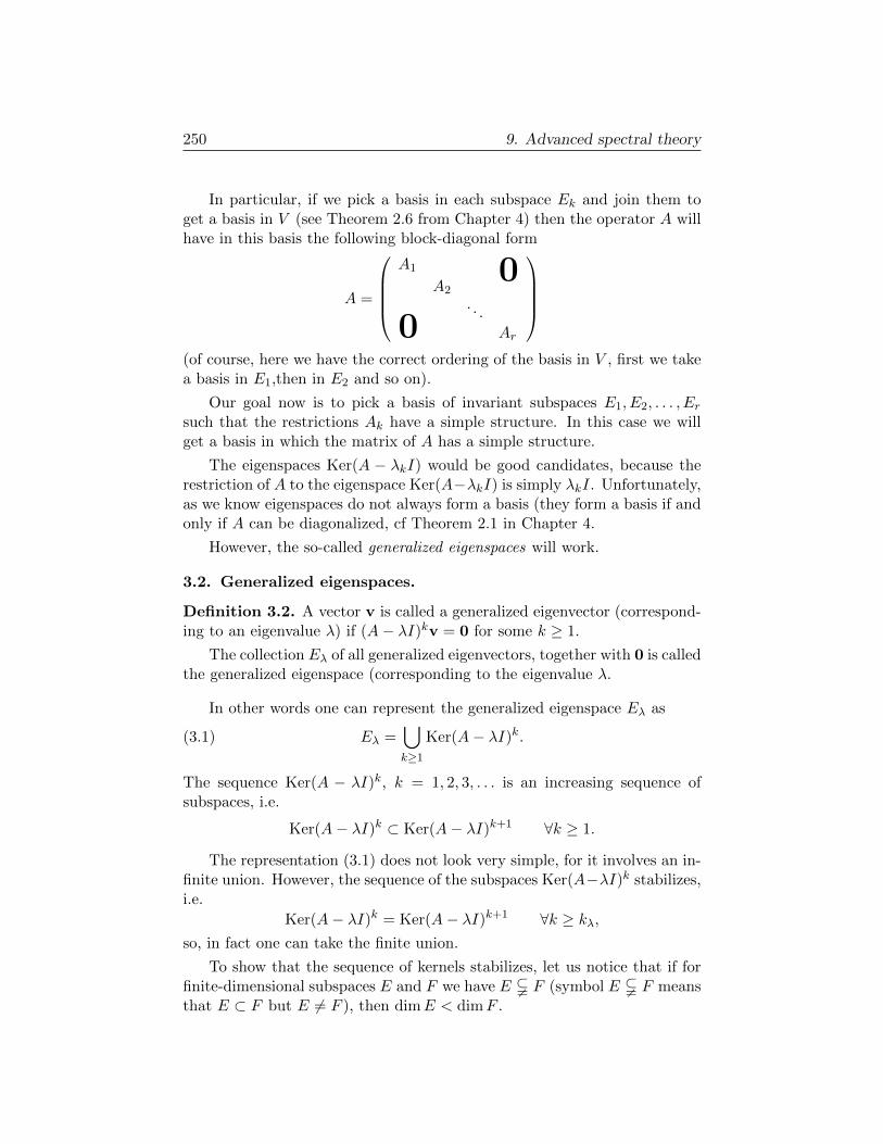
250 9. Advanced spectral theory

In particular, if we pick a basis in each subspace Ek and join them toget a basis in V (see Theorem 2.6 from Chapter 4) then the operator A willhave in this basis the following block-diagonal form

A =

A1

A20

. . .

0 Ar

(of course, here we have the correct ordering of the basis in V , first we takea basis in E1,then in E2 and so on).

Our goal now is to pick a basis of invariant subspaces E1, E2, . . . , Ersuch that the restrictions Ak have a simple structure. In this case we willget a basis in which the matrix of A has a simple structure.

The eigenspaces Ker(A − λkI) would be good candidates, because therestriction of A to the eigenspace Ker(A−λkI) is simply λkI. Unfortunately,as we know eigenspaces do not always form a basis (they form a basis if andonly if A can be diagonalized, cf Theorem 2.1 in Chapter 4.

However, the so-called generalized eigenspaces will work.

3.2. Generalized eigenspaces.

Definition 3.2. A vector v is called a generalized eigenvector (correspond-ing to an eigenvalue λ) if (A− λI)kv = 0 for some k ≥ 1.

The collection Eλ of all generalized eigenvectors, together with 0 is calledthe generalized eigenspace (corresponding to the eigenvalue λ.

In other words one can represent the generalized eigenspace Eλ as

(3.1) Eλ =⋃k≥1

Ker(A− λI)k.

The sequence Ker(A − λI)k, k = 1, 2, 3, . . . is an increasing sequence ofsubspaces, i.e.

Ker(A− λI)k ⊂ Ker(A− λI)k+1 ∀k ≥ 1.

The representation (3.1) does not look very simple, for it involves an in-finite union. However, the sequence of the subspaces Ker(A−λI)k stabilizes,i.e.

Ker(A− λI)k = Ker(A− λI)k+1 ∀k ≥ kλ,so, in fact one can take the finite union.

To show that the sequence of kernels stabilizes, let us notice that if forfinite-dimensional subspaces E and F we have E $ F (symbol E $ F meansthat E ⊂ F but E 6= F ), then dimE < dimF .

3. Generalized eigenspaces 251

Since dim Ker(A− λI)k ≤ dimV < ∞, it cannot grow to infinity, so atsome point

Ker(A− λI)k = Ker(A− λI)k+1.

The rest follows from the lemma below.

Lemma 3.3. Let for some k

Ker(A− λI)k = Ker(A− λI)k+1.

Then

Ker(A− λI)k+r = Ker(A− λI)k+r+1 ∀r ≥ 0.

Proof. Let v ∈ Ker(A− λI)k+r+1, i.e. (A− λI)k+r+1v = 0. Then

w := (A− λI)r ∈ Ker(A− λI)k+1.

But we know that Ker(A − λI)k = Ker(A − λI)k+1 so w ∈ Ker(A − λI)k,which means (A− λI)kw = 0. Recalling the definition of w we get that

(A− λI)k+rv = (A− λI)kw = 0

so v ∈ Ker(A−λI)k+r. We proved that Ker(A−λI)k+r+1 ⊂ Ker(A−λI)k+r.The opposite inclusion is trivial. �

Definition. The number d = d(λ) on which the sequence Ker(A − λI)k

stabilizes, i.e. the number d such that

Ker(A− λI)d−1 $ Ker(A− λI)d = Ker(A− λI)d+1

is called the depth of the eigenvalue λ.

It follows from the definition of the depth, that for the generalizedeigenspace Eλ

(3.2) (A− λI)d(λ)v = 0 ∀v ∈ Eλ.

Now let us summarize, what we know about generalized eigenspaces.

1. Eλ is an invariant subspace of A, AEλ ⊂ Eλ.

2. If d(λ) is the depth of the eigenvalue λ, then

((A− λI)|Eλ)d(λ) = (A|Eλ − λIEλ)d(λ) = 0.

(this is just another way of writing (3.2))

3. σ(A|Eλ) = {λ}, because the operator A|Eλ − λIEλ , is nilpotent, see2, and the spectrum of nilpotent operator consists of one point 0,see Problem 2.1

Now we are ready to state the main result of this section. Let A : V → V .

252 9. Advanced spectral theory

Theorem 3.4. Let σ(A) consists of r points λ1, λ2, . . . , λr, and let Ek :=Eλk be the corresponding generalized eigenspaces. Then the system of sub-space E1, E2, . . . , Er is a basis of subspaces in V .

Remark 3.5. If we join the bases in all generalized eigenspaces Ek, thenby Theorem 2.6 from Chapter 4 we will get a basis in the whole space.In this basis the matrix of the operator A has the block diagonal formA = diag{A1, A2, . . . , Ar}, where Ak := A|Ek , Ek = Eλk . It is also easy to

see, see (3.2) that the operators Nk := Ak − λkIEk are nilpotent, Ndkk = 0.

Proof of Theorem 3.4. Let mk be the multiplicity of the eigenvalue λk,so p(z) =

∏rk=1(z − λk)mk is the characteristic polynomial of A. Define

pk(z) = p(z)/(z − λk)mk =∏j 6=k

(z − λj)mj .

Lemma 3.6.

(3.3) (A− λkI)mk |Ek = 0,

Proof. There are 2 possible simple proofs. The first one is to notice thatmk ≥ dk, where dk is the depth of the eigenvalue λk and use the fact that

(A− λkI)dk |Ek = (Ak − λkIEk)mk = 0,

where Ak := A|Ek (property 2 of the generalized eigenspaces).

The second possibility is to notice that according to the Spectral Map-ping Theorem, see Corollary 2.2, the operator Pk(A)|Ek = pk(Ak) is invert-ible. By the Cayley–Hamilton Theorem (Theorem 1.1)

0 = p(A) = (A− λkI)mkpk(A),

and restriction all operators to Ek we get

0 = p(Ak) = (Ak − λkIEk)mkpk(Ak),

so(Ak − λkIEk)mk = p(Ak)pk(Ak)

−1 = 0 pk(Ak)−1 = 0.

�

To prove the theorem define

q(z) =

r∑k=1

pk(z).

Since pk(λj) = 0 for j 6= k and pk(λk) 6= 0, we can conclude that q(λk) 6= 0for all k. Therefore, by the Spectral Mapping Theorem, see Corollary 2.2,the operator

B = q(A)

is invertible.

3. Generalized eigenspaces 253

Note that BEk ⊂ Ek (any A-invariant subspace is also p(A)-invariant).Since B is an invertible operator, dim(BEk) = dimEk, which together withBEk ⊂ Ek implies BEk = Ek. Multiplying the last identity by B−1 we getthat B−1Ek = Ek, i.e. that Ek is an invariant subspace of B−1.

Note also, that it follows from (3.3) that

pk(A)|Ej = 0 ∀j 6= k,

because pk(A)|Ej = pk(Aj) and pk(Aj) contains the factor (Aj−λjIEj )mj =0.

Define the operators Pk by

Pk = B−1pk(A).

Lemma 3.7. For the operators Pk defined above

1. P1 + P2 + . . .+ Pr = I;

2. Pk|Ej = 0 for j 6= k;

3. RanPk ⊂ Ek;

4. moreover, Pkv = v ∀v ∈ Ek, so, in fact RanPk = Ek.

Proof. Property 1 is trivial:

r∑k=1

Pk = B−1r∑

k=1

Pkpk(A) = B−1B = I.

Property 2 follows from (3.3). Indeed, pk(A) contains the factor (A−λj)mj ,restriction of which to Ej is zero. Therefore pk(A)|Ej = 0 and thus Pk|Ej =

B−1pk(A)|Ej = 0.

To prove property 3, recall that according to Cayley–Hamilton Theoremp(A) = 0. Since p(z) = (z − λk)mkpk(z), we have for w = pk(A)v

(A− λkI)mkw = (A− λkI)mkpk(A)v = p(A)v = 0.

That means, any vector w in Ran pk(A) is annihilated by some power of(A− λkI), which by definition means that Ran pk(A) ⊂ Ek.

To prove the last property, let us notice that it follows from (3.3) thatfor v ∈ Ek

pk(A)v =

r∑j=1

pj(A)v = Bv,

which implies Pkv = B−1Bv = v. �

Now we are ready to complete the proof of the theorem. Take v ∈ Vand define vk = Pkv. Then according to Statement 3 of the above lemma,

254 9. Advanced spectral theory

vk ∈ Ek, and by Statement 1,

v =r∑

k=1

vk,

so v admits a representation as a linear combination.

To show that this representation is unique, we can just note, that if v isrepresented as v =

∑rk=1 vk, vk ∈ Ek, then it follows from the Statements

2 and 4 of the lemma that

Pkv = Pk(v1 + v2 + . . .+ vr) = Pkvk = vk.

�

3.3. Geometric meaning of algebraic multiplicity.

Proposition 3.8. Algebraic multiplicity of an eigenvalue equals the dimen-sion of the corresponding generalized eigenspace.

Proof. According to Remark 3.5, if we joint bases in generalized eigenspacesEk = Eλk to get a basis in the whole space, the matrix of A in any suchbasis has a block-diagonal form diag{A1, A2, . . . , Ar}, where Ak := A|Ek .Operators Nk = Ak − λkIEk are nilpotent, so σ(Nk) = {0}. Therefore,the spectrum of the operator Ak (recall that Ak = Nk − λkI) consists ofone eigenvalue λk of (algebraic) multiplicity nk = dimEk. The multiplicityequals nk because an operator in a finite-dimensional space V has exactlydimV eigenvalues counting multiplicities, and Ak has only one eigenvalue.

Note that we are free to pick bases in Ek, so let us pick them in such away that the corresponding blocks Ak are upper triangular. Then

det(A− λI) =

r∏k=1

det(Ak − λIEk) =

r∏k=1

(λk − λ)nk .

But this means that the algebraic multiplicity of the eigenvalue λk is nk =dimEλk . �

3.4. An important application. The following corollary is very impor-tant for differential equations.

Corollary 3.9. Any operator A in V can be represented as A = D + N ,where D is diagonalizable (i.e. diagonal in some basis) and N is nilpotent(Nm = 0 for some m), and DN = ND.

Proof. As we discussed above, see Remark 3.5, if we join the bases in Ekto get a basis in V , then in this basis A has the block diagonal form A =diag{A1, A2, . . . , Ar}, where Ak := A|Ek , Ek = Eλk . The operators Nk :=Ak−λkIEk are nilpotent, and the operatorD = diag{λ1IE1 , λ2IE2 . . . , λrIEr}

3. Generalized eigenspaces 255

is diagonal (in this basis). Notice also that λkIEkNk = NkλkIEk (iden-tity operator commutes with any operator), so the block diagonal operatorN = diag{N1, N2, . . . , Nr} commutes with D, DN = ND. Therefore, defin-ing N as the block diagonal operator N = diag{N1, N2, . . . , Nr} we get thedesired decomposition. �

This corollary allows us to compute functions of operators. Let us recallthat if p is a polynomial of degree d, then p(a + x) can be computed withthe help of Taylor’s formula

p(a+ x) =d∑

k=0

p(k)(a)

k!xk

This formula is an algebraic identity, meaning that for each polynomial pwe can check that the formula is true using formal algebraic manipulationswith a and x and not caring about their nature.

Since operators D and N commute, DN = ND, the same rules as forusual (scalar) variables apply to them, and we can write (by plugging Dinstead of a and N instead of x

p(A) = p(D +N) =

d∑k=0

p(k)(D)

k!Nk.

Here, to compute the derivative p(k)(D) we first compute the kth derivativeof the polynomial p(x) (using the usual rules from calculus), and then plugD instead of x.

But since N is nilpotent, Nm = 0 for some m, only first m terms canbe non-zero, so

p(A) = p(D +N) =m−1∑k=0

f (k)(D)

k!Nk.

In m is much smaller than d, this formula makes computation of p(A) mucheasier.

The same approach works if p is not a polynomial, but an infinite powerseries. For general power series we have to be careful about convergenceof all the series involved, so we cannot say that the formula is true for anarbitrary power series p(x). However, if the radius of convergence of thepower series is ∞, then everything works fine. In particular, if p(x) = ex,then, using the fact that (ex)′ = ex we get.

eA =m−1∑k=0

eD

k!Nk = eD

m−1∑k=0

1

k!Nk

This formula has important applications in differential equation.

256 9. Advanced spectral theory

Note, that the fact that ND = DN is essential here!

4. Structure of nilpotent operators

Recall, that an operator A in a vector space V is called nilpotent if Ak = 0for some exponent k.

In the previous section we have proved, see Remark 3.5, that if we jointhe bases in all generalized eigenspaces Ek = Eλk to get a basis in thewhole space, then the operator A has in this basis a block diagonal formdiag{A1, A2, . . . , Ar} and operators Ak ca be represented as Ak = λkI+Nk,where Nk are nilpotent operators.

In each generalized eigenspace Ek we want to pick up a basis such thatthe matrix of Ak in this basis has the simplest possible form. Since matrix(in any basis) of the identity operator is the identity matrix, we need to finda basis in which the nilpotent operator Nk has a simple form.

Since we can deal with each Nk separately, we will need to consider thefollowing problem:

For a nilpotent operator A find a basis such that the matrixof A in this basis is simple.

Let see, what does it mean for a matrix to have a simple form. It is easy tosee that the matrix

(4.1)

0 1 0

0 1

0. . .. . . 1

0 0

is nilpotent.

These matrices (together with 1× 1 zero matrices) will be our “buildingblocks”. Namely, we will show that for any nilpotent operator one can finda basis such that the matrix of the operator in this basis has the blockdiagonal form diag{A1, A2, . . . , Ar}, where each Ak is either a block of form(4.1) or a 1× 1 zero block.

Let us see what we should be looking for. Suppose the matrix of anoperator A has in a basis v1,v2, . . . ,vp the form (4.1). Then

Av1 = 0(4.2)

and

Avk+1 = vk, k = 1, 2, . . . , p− 1.(4.3)

4. Structure of nilpotent operators 257

Thus we have to be looking for the chains of vectors v1,v2, . . . ,vp satisfyingthe above relations (4.2), (4.3).

4.1. Cycles of generalized eigenvectors.

Definition. Let A be a nilpotent operator. A chain of non-zero vectorsv1,v2, . . . ,vp satisfying relations (4.2), (4.3) is called a cycle of generalizedeigenvectors of A. The vector v1 is called the initial vector of the cycle, thevector vp is called the end vector of the cycle, and the number p is calledthe length of the cycle.

Remark. A similar definition can be made for an arbitrary operator. Thenall vectors vk must belong to the same generalized eigenspace Eλ, and theymust satisfy the identities

(A− λI)v1 = 0, (A− λI)vk+1 = vk, k = 1, 2, . . . , p− 1,

Theorem 4.1. Let A be a nilpotent operator, and let C1, C2, . . . , Cr be cyclesof its generalized eigenvectors, Ck = vk1 ,v

k2 , . . . ,v

kpk

, pk being the length of

the cycle Ck. Assume that the initial vectors v11,v

21, . . . ,v

r1 are linearly in-

dependent. Then no vector belongs to two cycles, and the union of all thevectors from all the cycles is a linearly independent.

Proof. Let n = p1 + p2 + . . .+ pr be the total number of vectors in all thecycles2. We will use induction in n. If n = 1 the theorem is trivial.

Let us now assume, that the theorem is true for all operators and for allcollection of cycles, as long as the total number of vectors in all the cyclesis strictly less than n.

Without loss of generality we can assume that the vectors vkj span thewhole space V , because, otherwise we can consider instead of the operatorA its restriction onto the invariant subspace span{vkj : k = 1, 2, . . . , r, 1 ≤j ≤ pk}.

Consider the subspace RanA. It follows from the relations (4.2), (4.3)that vectors vkj : k = 1, 2, . . . , r, 1 ≤ j ≤ pk − 1 span RanA. Note that if

pk > 1 then the system vk1 ,vk2 , . . . ,v

kpk−1 is a cycle, and that A annihilates

any cycle of length 1.

Therefore, we have finitely many cycles, and initial vectors of these cyclesare linearly independent, so the induction hypothesis applies, and the vectorsvkj : k = 1, 2, . . . , r, 1 ≤ j ≤ pk − 1 are linearly independent. Since thesevectors also span RanA, we have a basis there. Therefore,

rankA = dim RanA = n− r2Here we just count vectors in each cycle, and add all the numbers. We do not care if some

cycles have a common vector, we count this vector in each cycle it belongs to (of course, accordingto the theorem, it is impossible, but initially we cannot assume that)

258 9. Advanced spectral theory

(we had n vectors, and we removed one vector vkpk from each cycle Ck,k = 1, 2, . . . , r, so we have n− r vectors in the basis vkj : k = 1, 2, . . . , r, 1 ≤j ≤ pk − 1 ). On the other hand Avk1 = 0 for k = 1, 2, . . . , r, and since thesevectors are linearly independent dim KerA ≥ r. By the Rank Theorem(Theorem 7.1 from Chapter 2)

dimV = rankA+ dim KerA = (n− r) + dim KerA ≥ (n− r) + r = n

so dimV ≥ n.

On the other hand V is spanned by n vectors, therefore the vectors vkj :k = 1, 2, . . . , r, 1 ≤ j ≤ pk, form a basis, so they are linearly independent �

4.2. Jordan canonical form of a nilpotent operator.

Theorem 4.2. Let A : V → V be a nilpotent operator. Then V has a basisconsisting of union of cycles of generalized eigenvectors of the operator A.

Proof. We will use induction in n where n = dimV . For n = 1 the theoremis trivial.

Assume that the theorem is true for any operator acting in a space ofdimension strictly less than n.

Consider the subspace X = RanA. X is an invariant subspace of theoperator A, so we can consider the restriction A|X .

Since A is not invertible, dim RanA < dimV , so by the induction hy-pothesis there exist cycles C1, C2, . . . , Cr of generalized eigenvectors such thattheir union is a basis in X. Let Ck = vk1 ,v

k2 , . . . ,v

kpk

, where vk1 is the initialvector of the cycle.

Since the end vector vkpk belong to RanA, one can find a vector vkpk+1

such that Avpk+1 = vkpk . So we can extend each cycle Ck to a bigger cycle

Ck = vk1 ,vk2 , . . . ,v

kpk,vkpk+1. Since the initial vectors vk1 of cycles Ck, k =

1, 2, . . . , r are linearly independent, the above Theorem 4.1 implies that theunion of these cycles is a linearly independent system.

By the definition of the cycle we have vk1 ∈ KerA, and we assumedthat the initial vectors vk1 , k = 1, 2, . . . , r are linearly independent. Let uscomplete this system to a basis in KerA, i.e. let find vectors u1,u2, . . . ,uqsuch that the system v1

1,v21, . . . ,v

r1,u1,u2, . . . ,uq is a basis in KerA (it may

happen that the system vk1 , k = 1, 2, . . . , r is already a basis in KerA, inwhich case we put q = 0 and add nothing).

The vector uj can be treated as a cycle of length 1, so we have a collec-

tion of cycles C1, C2, . . . , Cr,u1,u2, . . . ,uq, whose initial vectors are linearlyindependent. So, we can apply Theorem 4.1 to get that the union of allthese cycles is a linearly independent system.

4. Structure of nilpotent operators 259

To show that it is a basis, let us count the dimensions. We know thatthe cycles C1, C2, . . . , Cr have dim RanA = rankA vectors total. Each cycle

Ck was obtained from Ck by adding 1 vector to it, so the total number of

vectors in all the cycles Ck is rankA+ r.

We know that dim KerA = r + q (because v11,v

21, . . . ,v

r1,u1,u2, . . . ,uq

is a basis there). We added to the cycles C1, C2, . . . , Cr additional q vectors,so we got

rankA+ r + q = rankA+ dim KerA = dimV

linearly independent vectors. But dimV linearly independent vectors is abasis. �

Definition. A basis consisting of a union of cycles of generalized eigen-vectors of a nilpotent operator A (existence of which is guaranteed by theTheorem 4.2) is called a Jordan canonical basis for A.

Note, that such basis is not unique.

Corollary 4.3. Let A be a nilpotent operator. There exists a basis (a Jordancanonical basis) such that the matrix of A in this basis is a block diagonaldiag{A1, A2, . . . , Ar}, where all Ak (except may be one) are blocks of form(4.1), and one of the blocks Ak can be zero.

The matrix of A in a Jordan canonical basis is called the Jordan canoni-cal form of the operator A. We will see later that the Jordan canonical formis unique, if we agree on how to order the blocks (i.e. on how to order thevectors in the basis).

Proof of Corollary 4.3. According to Theorem 4.2 one can find a basisconsisting of a union of cycles of generalized eigenvectors. A cycle of sizep gives rise to a p × p diagonal block of form (4.1), and a cycle of length 1correspond to a 1× 1 zero block. We can join these 1× 1 zero blocks in onelarge zero block (because off-diagonal entries are 0). �

4.3. Dot diagrams. Uniqueness of the Jordan canonical form.There is a good way of visualizing Theorem 4.2 and Corollary 4.3, the so-called dot diagrams. This methods also allows us to answer many naturalquestions, like “is the block diagonal representation given by Corollary 4.3unique?”

Of course, if we treat this question literally, the answer is “no”, for wealways can change the order of the blocks. But, if we exclude such trivialpossibilities, for example by agreeing on some order of blocks (say, if we putall non-zero blocks in decreasing order, and then put the zero block), is therepresentation unique, or not?

260 9. Advanced spectral theory

r r r r r rr r rr r rrr

0 10 1

0 10 1 0

0 00 1

0 10 0

0 10 1

0 00

00

Figure 1. Dot diagram and corresponding Jordan canonical form of anilpotent operator

To better understand the structure of nilpotent operators, described inthe Section 4.1, let us draw the so-called dot diagram. Namely, suppose wehave a basis, which is a union of cycles of generalized eigenvalues. Let usrepresent the basis by an array of dots, so that each column represents acycle. The first row consists of initial vectors of cycles, and we arrange thecolumns (cycles) by their length, putting the longest one to the left.

On the figure 1 we have the dot diagram of a nilpotent operator, as wellas its Jordan canonical form. This dot diagram shows, that the basis has 1cycle of length 5, two cycles of length 3, and 3 cycles of length 1. The cycleof length 5 corresponds to the 5× 5 block of the matrix, the cycles of length3 correspond to two 3 non-zero blocks. Three cycles of length 1 correspondto three zero entries on the diagonal, which we join in the 3× 3 zero block.Here we only giving the main diagonal of the matrix and the diagonal aboveit; all other entries of the matrix are zero.

If we agree on the ordering of the blocks, there is a one-to-one corre-spondence between dot diagrams and Jordan canonical forms (for nilpotentoperators). So, the question about uniqueness of the Jordan canonical formis equivalent to the question about uniqueness of the dot diagram.

To answer this question, let us analyze, how the operator A transformsthe dot diagram. Since the operator A annihilates initial vectors of thecycles, and moves vector vk+1 of a cycle to the vector vk, we can see thatthe operator A acts on its dot diagram by deleting the first (top) row of thediagram.

4. Structure of nilpotent operators 261

The new dot diagram corresponds to a Jordan canonical basis in RanA,and allows us to write down the Jordan canonical form for the restrictionA|RanA.

Similarly, it is not hard to see that the operator Ak removes the firstk rows of the dot diagram. Therefore, if for all k we know the dimensionsdim Ker(Ak), we know the dot diagram of the operator A. Namely, thenumber of dots in the first row is dim KerA, the number of dots in thesecond row is

dim Ker(A2)− dim KerA,

and the number of dots in the kth row is

dim Ker(Ak)− dim Ker(Ak+1).

But this means that the dot diagram, which was initially defined usinga Jordan canonical basis, does not depend on a particular choice of such abasis. Therefore, the dot diagram, is unique! This implies that if we agreeon the order of the blocks, then the Jordan canonical form is unique.

4.4. Computing a Jordan canonical basis. Let us say few words aboutcomputing a Jordan canonical basis for a nilpotent operator. Let p1 be thelargest integer such that Ap1 6= 0 (so Ap1+1 = 0). One can see from theabove analysis of dot diagrams, that p1 is the length of the longest cycle.

Computing operators Ak, k = 1, 2, . . . , p1, and counting dim Ker(Ak) wecan construct the dot diagram of A. Now we want to put vectors instead ofdots and find a basis which is a union of cycles.

We start by finding the longest cycles (because we know the dot diagram,we know how many cycles should be there, and what is the length of eachcycle). Consider a basis in the column space Ran(Ap1). Name the vectorsin this basis v1

1,v21, . . . ,v

r11 , these will be the initial vectors of the cycles.

Then we find the end vectors of the cycles v1p1 ,v

2p1 , . . . ,v

r1p1 by solving the

equations

Ap1vkp1 = vk1 , k = 1, 2, . . . , r1.

Applying consecutively the operator A to the end vector vkp1 , we get all the

vectors vkj in the cycle. Thus, we have constructed all cycles of maximallength.

Let p2 be the length of a maximal cycle among those that are left tofind. Consider the subspace Ran(Ap2), and let dim Ran(Ap2) = r2. SinceRan(Ap1) ⊂ Ran(Ap2), we can complete the basis v1

1,v21, . . . ,v

r11 to a basis

v11,v

21, . . . ,v

r11 ,v

r1+11 , . . . ,vr21 in Ran(Ar2). Then we find end vectors of the

cycles Cr1+1, . . . , Cr2 by solving (for vkp2) the equations

Ap1vkp2 = vk1 , k = r1 + 1, r1 + 2, . . . , r2,

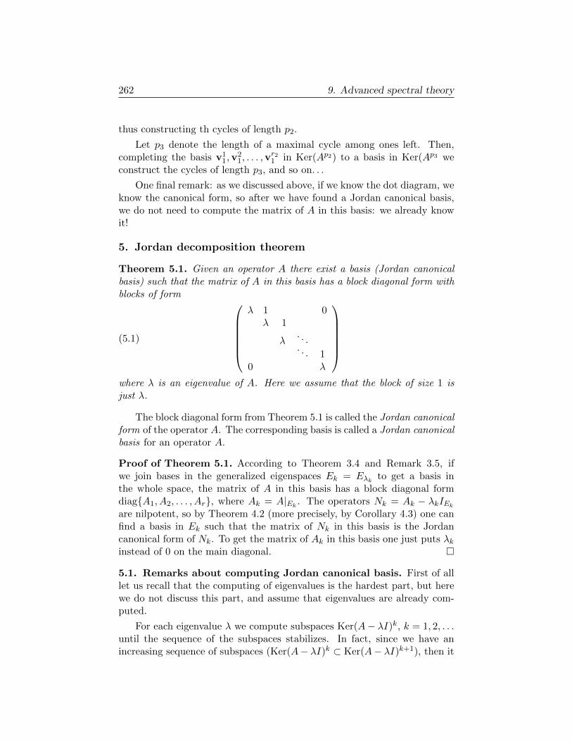
262 9. Advanced spectral theory

thus constructing th cycles of length p2.

Let p3 denote the length of a maximal cycle among ones left. Then,completing the basis v1

1,v21, . . . ,v

r21 in Ker(Ap2) to a basis in Ker(Ap3 we

construct the cycles of length p3, and so on. . .

One final remark: as we discussed above, if we know the dot diagram, weknow the canonical form, so after we have found a Jordan canonical basis,we do not need to compute the matrix of A in this basis: we already knowit!

5. Jordan decomposition theorem

Theorem 5.1. Given an operator A there exist a basis (Jordan canonicalbasis) such that the matrix of A in this basis has a block diagonal form withblocks of form

(5.1)

λ 1 0

λ 1

λ. . .. . . 1

0 λ

where λ is an eigenvalue of A. Here we assume that the block of size 1 isjust λ.

The block diagonal form from Theorem 5.1 is called the Jordan canonicalform of the operator A. The corresponding basis is called a Jordan canonicalbasis for an operator A.

Proof of Theorem 5.1. According to Theorem 3.4 and Remark 3.5, ifwe join bases in the generalized eigenspaces Ek = Eλk to get a basis inthe whole space, the matrix of A in this basis has a block diagonal formdiag{A1, A2, . . . , Ar}, where Ak = A|Ek . The operators Nk = Ak − λkIEkare nilpotent, so by Theorem 4.2 (more precisely, by Corollary 4.3) one canfind a basis in Ek such that the matrix of Nk in this basis is the Jordancanonical form of Nk. To get the matrix of Ak in this basis one just puts λkinstead of 0 on the main diagonal. �

5.1. Remarks about computing Jordan canonical basis. First of alllet us recall that the computing of eigenvalues is the hardest part, but herewe do not discuss this part, and assume that eigenvalues are already com-puted.

For each eigenvalue λ we compute subspaces Ker(A− λI)k, k = 1, 2, . . .until the sequence of the subspaces stabilizes. In fact, since we have anincreasing sequence of subspaces (Ker(A− λI)k ⊂ Ker(A− λI)k+1), then it

5. Jordan decomposition theorem 263

is sufficient only to keep track of their dimension (or ranks of the operators(A − λI)k). For an eigenvalue λ let m = mλ be the number where thesequence Ker(A− λI)k stabilizes, i.e. m satisfies

dim Ker(A− λI)m−1 < dim Ker(A− λI)m = dim Ker(A− λI)m+1.

Then Eλ = Ker(A−λI)m is the generalized eigenspace corresponding to theeigenvalue λ.

After we computed all the generalized eigenspaces there are two possibleways of action. The first way is to find a basis in each generalized eigenspace,so the matrix of the operator A in this basis has the block-diagonal formdiag{A1, A2, . . . , Ar}, where Ak = A|Eλk . Then we can deal with each ma-

trix Ak separately. The operators Nk = Ak −λkI are nilpotent, so applyingthe algorithm described in Section 4.4 we get the Jordan canonical repre-sentation for Nk, and putting λk instead of 0 on the main diagonal, we getthe Jordan canonical representation for the block Ak. The advantage of thisapproach is that we are working with smaller blocks. But we need to findthe matrix of the operator in a new basis, which involves inverting a matrixand matrix multiplication.

Another way is to find a Jordan canonical basis in each of the generalizedeigenspaces Eλk by working directly with the operator A, without splittingit first into the blocks. Again, the algorithm we outlined above in Section4.4 works with a slight modification. Namely, when computing a Jordancanonical basis for a generalized eigenspace Eλk , instead of considering sub-spaces Ran(Ak−λkI)j , which we would need to consider when working withthe block Ak separately, we consider the subspaces (A− λkI)jEλk .

Index

Mm,n, 3

Mm×n, 3

δk,j , see Kroneker delta

adjoint

of an operator, 138

basis, 6

biorthogonal, see basis, dual

dual, 210

of subspaces, 107

orthogonal, 125

orthonormal, 125

coordinates

of a vector in the basis, 6

counting multiplicities, 102

dual basis, 210

dual space, 207

duality, 233

eigenvalue, 100

eigenvector, 100

Einstein notation, 226, 235

entry, entries

of a matrix, 4

of a tensor, 238

Fourier decomposition

abstract, non-orthogonal, 212, 216

abstract, orthogonal, 125, 217

Frobenius norm, 175

functional

linear, 207

generalized eigenspace, 250

generalized eigenvector, 250

generating system, 7

Gram–Schmidt orthogonalization, 129

Hermitian matrix, 159

Hilbert–Schmidt norm, 175

inner product

abstract, 117

in Cn, 116

inner product space, 117

invariant subspace, 245

isometry, 142

Jordan canonical

basis, 259, 262

form, 259, 262

basis

for a nilpotent operator, 259

form

for a nilpotent operator, 259

Jordan decomposition theorem, 262

for a nilpotent operator, 259

Kroneker delta, 210, 216

least square solution, 133

linear combination, 6

trivial, 8

linear functional, 207

linearly dependent, 8

linearly independent, 8

matrix, 4

antisymmetric, 11

265

266 Index

lower triangular, 81symmetric, 5, 11

triangular, 81

upper triangular, 31, 81minor, 95

multilinear function, 229multilinear functional, see tensor

multiplicities

counting, 102multiplicity

algebraic, 102

geometric, 102

norm

operator, 175normal operator, 161

operator norm, 175orthogonal complement, 131

orthogonal projection, 127

polynomial matrix, 94

projectionorthogonal, 127

self-adjoint operator, 159space

dual, 207

Spectral theory, 99spectrum, 100

submatrix, 95

subspaceinvariant, 245

tensor, 229r-covariant s-contravariant, 233

contravariant, 233covariant, 233

trace, 22

transpose, 4triangular matrix, 81

eigenvalues of, 103

unitary operator, 143

valencyof a tensor, 229