Generated using version 3.0 of the official AMS LATEX template

Detecting the ITCZ in instantaneous satellite data using

spatial-temporal statistical modeling: ITCZ climatology in the

east Pacific

Caroline L. Bain ∗ , Jorge De Paz, Jason Kramer,

Gudrun Magnusdottir, Padhraic Smyth,

Hal Stern and Chia-chi Wang†

University of California, Irvine, USA

∗Corresponding author address: Caroline Bain c/o Gudrun Magnusdottir, Department of Earth System

Science, University of California, Irvine, CA 92697.

E-mail: gudrun@uci.edu†now at: Department of Atmospheric Sciences, Chinese Culture University, Taipei, Taiwan

1

ABSTRACT

A Markov random field (MRF) statistical model is introduced, developed and validated for

detecting the east Pacific Intertropical Convergence Zone (ITCZ) in instantaneous satellite

data from May through October. The MRF statistical model uses satellite data at a given

location as well as information from its neighboring points (in time and space) to decide

whether the given point is classified as ITCZ or non-ITCZ. Two different labels of ITCZ

occurrence are produced. IR-only labels result from running the model with 3-hourly in-

frared data available for a 30 yr period, 1980–2009. Data-all labels result from running the

model with additional satellite data (visible and total precipitable water), available from

1995–2008. IR-only labels detect less area of ITCZ than Data-all labels, especially where

the ITCZ is shallower. Yet, qualitatively, the results for the two sets of labels are similar.

The seasonal distribution of the ITCZ through the summer half year is presented, showing

typical location and extent. The ITCZ is mostly confined to the eastern Pacific in May, and

becomes more zonally distributed towards September and October each year. Northward

and westward shifts in the location of the ITCZ occur in line with the seasonal cycle and

warm sea surface temperatures. The ITCZ is quite variable on interannual time scales and

highly correlated with ENSO variability. When we removed the ENSO signal from labels,

interannual variability remained high. The resulting IR-only labels, representing the longer

time series, showed no evidence of a trend in location nor evidence of a trend in area for the

30 yr period.

1

1. Introduction

The Intertropical Convergence Zone (ITCZ) is one of the most recognizable aspects of the

global circulation that can be seen from space. The ITCZ forms as a zonally elongated band

of cloud at low latitudes, where the northeasterly and southeasterly trade winds converge.

The focus of this paper is to introduce a new method which detects the ITCZ using high

temporal and spatial resolution satellite products that have recently been archived. We

apply the method in the Pacific region north of the equator and east of the dateline during

the boreal summer half year (May through October, hereafter summer).

Previous observational studies of the global climatological ITCZ (e.g. Mitchell and Wal-

lace 1992; Waliser and Gautier 1993) focused on the annual cycle in different regions. They

found very distinct longitudinal variations in the ITCZ. In the Indo- western Pacific region

the summer ITCZ is broad in latitude and ill-defined due to the extensive warm pool in the

ocean and monsoonal circulations. However, in the east Pacific the mean summer ITCZ is

narrow and long, generally located at the southern boundary of the east Pacific warm pool,

north of the strongest meridional gradient of sea surface temperature (Raymond et al. 2003).

During the summer the east Pacific ITCZ is particularly visible in instantaneous satellite

fields. During northern hemisphere winter the ITCZ remains in the northern hemisphere,

but its signature is considerably weaker and gets mixed in with signatures of extratropical

frontal systems due to cold air outbreaks (Wang and Magnusdottir 2006, hereafter WM06).

Traditionally, the ITCZ has been identified in terms of time-averaged fields, either in

terms of the seasonal mean outgoing longwave radiation (OLR), or, in more recent years,

in terms of the seasonal mean precipitation. For example (Waliser and Gautier 1993) used

2

thresholding of mean OLR in combination with mean high reflectivity to identify the ITCZ.

A low OLR threshold is chosen, and values below this threshold are considered to represent

clouds that are part of the convection within the ITCZ. To filter out smaller systems an

area limit is often imposed. Little attempt has been made to date to group the low OLR

clouds into a continuous zonally elongated feature, nor to remove noise and accommodate

shallower convection which often characterizes the narrow east Pacific ITCZ region (Zhang

et al. 2004).

Other studies (e.g. Serra and Houze 2002), have referred to the ITCZ as a geographical

region along which westward propagating disturbances (WPDs) tend to propagate zonally.

Weak WPDs (or easterly waves) have been observed to propagate through the ITCZ cloud en-

velope (e.g. Scharenbroich et al. 2010) and in general it is impractical to attempt to separate

the signal of easterly wave out of the ITCZ signal. Magnusdottir and Wang (2008) reached

the same conclusion when using spectral analysis on ERA-40 850hPa relative vorticity. The

line of thinking that easterly waves or WPDs are inseparable from the ITCZ accommodates

the idea that the ITCZ is composed of WPDs, but Gu and Zhang (2002a,b) demonstrated

there is an additional important component to the ITCZ that is not propagating.

Satellite images show that from day to day the ITCZ is highly dynamic and changeable.

The ITCZ can form as a narrow band of convection stretched over an extensive longitudinal

distance (up to 70◦) for hours to days, until its structure breaks down into individual distur-

bances that may move away or dissipate in place. The ITCZ envelope of convection usually

reforms within a day or two of breakdown (WM06). This dynamic ITCZ has been the sub-

ject of dynamical modeling studies (Ferreira and Schubert 1997a; Wang and Magnusdottir

2005; Wang et al. 2010) that concluded that barotropic instability was important in ITCZ

3

breakdown.

The variability in the ITCZ presents a serious challenge to its automatic detection in

instantaneous data. Here we want to focus on the ITCZ as a weather feature that has long

been recognized by satellite meteorologists who analyze instantaneous fields. We use the

following criteria to define the ITCZ:

i. The ITCZ is a predominantly zonal feature.

ii. It is cloudy but there may be cloud-free regions within the envelope of convection and

the convection may be shallow (as represented by rather warm cloud top temperatures).

iii. The ITCZ is a large-scale feature and isolated tropical disturbances, unconnected to

larger cloudy regions, are not part of the ITCZ.

We use satellite fields of infrared (IR), visible (VS) and total precipitable water (TPW) to

find large-scale zonally connected regions of convection.

WM06 present a detailed study of daily variability of the ITCZ in the east Pacific for

five years, 1999-2003, using visual inspection of satellite images. Here we extend their study

by presenting a new method to automate the detection so that a greater number of active

seasons may be analyzed. The new method is based on a statistical model that will produce

the same results given the same data, which may not be true for human identification of the

ITCZ. In other respects, the model seeks to emulate human analysis of the meteorological

feature; looking for continuity in space and time while accommodating different meteorolog-

ical fields. The output from the statistical model is a binary field, referred to as ITCZ labels,

representing the presence (by 1) or absence (by 0) of the ITCZ in the area of interest at each

time point. In this paper we introduce and validate the statistical model as well as present

4

first results focusing mainly on the climatology of the ITCZ, its interannual variability and

seasonal evolution.

The paper is organized as follows: Section 2 describes the input satellite data, section

3 the statistical model and section 4 evaluates our approach to ITCZ detection. Section 5

presents results from two different outputs from the model: a longer (1980–2009) time series

of ITCZ labels obtained using IR data only, and a shorter (1995–2008) time series of labels

obtained using all three sources of data (IR, VS and total precipitable water, TPW). Finally,

section 6 presents concluding remarks.

2. Satellite Data

Satellite IR, VS, and TPW images from 90–180◦W were used for analysis. The VS data

are a measure of reflectivity of clouds, the IR data correspond to cloud-top temperature.

The TPW data give the water vapor content of the entire column in units of equivalent

thickness of liquid water (0–75 mm).

The IR and VS data sets were obtained from the National Climatic Data Center (NCDC)

of NOAA. These two data sets are from the HURSAT Basin data (Knapp 2008) and are

closely related to HURSAT B1 data (Knapp and Kossin 2007), which are derived from ISCCP

B1 data. The data were collected from radiometers on different geostationary satellites. The

IR channel data were recalibrated to reduce inter-satellite differences. The HURSAT Basin

data have the same spatial and temporal resolution as HURSAT B1 data, but are assembled,

gridded and archived for each tropical ocean basin separately1. The IR data set is available

1for more information see www.ncdc.noaa.gov/oa/rsat/hursat

5

every three hours (00 UTC etc.) from 1980-2009 at a spatial resolution of 10 km. We chose

to reduce the spatial resolution of the satellite fields to 0.5◦ in order to reduce the number

of grid points and decrease computation time. Coarsening the grid does not influence the

end result as the ITCZ objects we identify are considerably larger.

The longitudinal extent of our domain (90-180◦W) means that the entire area is in day-

light only once per day (21 UTC) even though global VS data are available every three

hours. Thus the VS data set is only useful once per day, however the statistical model is

able to accommodate for the missing measurements. We also found that the earlier parts of

the record were problematic for the VS channel, therefore the VS data set is only used from

1995–2008.

The TPW data was assembled and archived by Remote Sensing Systems2. The data is a

composite of available microwave data (from the SSM/I, TMI, AMSR-E satellites). It covers

1987–2008, however the earlier part of the record is at lower temporal resolution so we only

use the data for 1995–2008. The data is at a spatial resolution of 0.25◦ that we coarsen to

0.5◦. The images are from 00, 06, 12, 18 UTC and contain data from ± 3 hours, in practice

making them ± 9 hours resolution at each recorded time point. Furthermore, we applied

linear interpolation between the time points, making TPW available at the same time as IR.

To summarize, one data set, IR, is available from 1980–2009. The other two data sets,

VS and TPW, are used for the latter part of the time period or 1995–2008. We therefore

chose to run our analysis of the east Pacific ITCZ twice. First using all three satellite data

sets for the period 1995–2008. Secondly, we ran our analysis for the entire time period,

1980–2009, using the IR data only.

2www.remss.com

6

Since there are two versions of the model with different inputs, it is critical that we have

consistent terminology to identify the output. The term ‘All-data labels’ refers to the set of

ITCZ labels obtained from the MRF model using IR, VS and TPW satellite data as input.

The term ‘IR-only labels’ refers to the set of ITCZ labels obtained from the MRF model

using only IR for input.

3. Method description

The statistical model used to detect the ITCZ incorporates satellite data, a Markov

random field (MRF) that represents ITCZ/ non-ITCZ, and ‘a priori’ information on the

most likely location of the ITCZ. In the following explanation we will use Xijt as an indicator

of the presence (Xijt = 1) or absence (Xijt = 0) of the ITCZ at longitude i, latitude j, and

discretized time t. The corresponding satellite data will be denoted Yijt, a vector comprised

of satellite IR, VS and TPW. Xijt is not directly observable since the ITCZ is not defined

deterministically as a function of satellite data (such as clouds below some temperature are

always ITCZ etc.). Thus, the binary status of ITCZ at each grid point is instead inferred from

satellite data, Yijt, and the status of surrounding grid points in time and space. The final

ITCZ status of each grid point is determined by sampling from the posterior distribution:

P (X|Y ) =P (Y |X)P (X)∑X P (Y |X)P (X)

(1)

where P (Y |X) gives the likelihood of the satellite data Y , given X (ITCZ or non-ITCZ

status). P (X) is a prior distribution on the probability of ITCZ that incorporates nieghbor-

7

hood and spatial information. We describe the specifics of this model, our computational

approach, and other implementation details in the remainder of this section.

a. Learning the distribution of satellite data, P (Y |X)

The model requires knowledge of the satellite values which are characteristic of ITCZ and

non-ITCZ. This information was obtained from training data provided by manual labelling of

satellite data. Three meteorologists identified closed ITCZ regions (if any) at 2100 UTC for

each day during August 2000. The labellers were provided with a graphical user interface

and a tablet board with stylus to maximize precision when labelling the region desired.

They were given VS, IR and TPW at times t − 2, t − 1, t, t + 1 and t + 2 where t was the

time-frame being labelled. The individuals using the tablet board were told to label based

on principles listed in the introduction (section 1). Continuity in time and reconciling the

different meteorological fields are important elements in the manual labeling and constitute

what the statistical model seeks to emulate.

The mean vector and covariance matrix for VS, IR, and TPW, for grid points belonging

to the ITCZ (X = 1) and non-ITCZ (X = 0) were created using the manual labelled data.

The means and covariances were used to produce two Gaussian distributions for the satellite

data Y , conditioned on X = 1 and X = 0. These distributions (for each of VS, IR and

TPW) had different means and variances for ITCZ (X = 1) and non-ITCZ (X = 0), but

also overlapped. If the satellite data at a given grid point falls within the overlap regions,

there is less certainty as to whether X = 1 or X = 0. The Gaussian distribution for X = 1

is less broad than the one for X = 0, as the ITCZ is mostly cloudy, whereas the non-ITCZ is

8

a mixture of cloud and non-cloud. It is assumed that given X, the observed satellite values,

Y , are independent across different grid points and times, so that

P (Y |X) =∏

ijt

P (Yijt|Xijt). (2)

The set of manual labels which performed best against the union of labels (Person 1,

see table 1) was used to train the statistical model. Additional months were subsequently

labelled to check that P (Y |X) did not change significantly, but these labels were not used

for training the final model.

b. A Markov random field model for the ITCZ, P (X)

The Markov random field (MRF) is a mathematical model (Kindermann and Snell 1980;

Geman and Geman 1984; Li 1994; Smyth 1997) that specifies a probability distribution on

the spatial characteristics of the ITCZ. The MRF allows us to incorporate typical spatial

locations for the ITCZ along with the informal notion that if one grid point is part of the

ITCZ then this ought to increase the likelihood that neighboring grid points are also part of

the ITCZ.

In an MRF model the status of a single grid point, Xijt, depends only on grid points that

are immediate neighbors. If we define Nijt as the set of neighbors of Xijt, and X−ijt as the

set of all grid points except our initial grid point, then the Markov property says that

P (Xijt|X−ijt) = P (Xijt|Nijt). (3)

The neighborhood that we use includes the immediate neighbors in the longitude (Xi+1,j,t, Xi−1,j,t),

latitude, (Xi,j+1,t, Xi,j−1,t), and time (Xi,j,t+1, Xi,j,t−1) directions. Figure 1 is a schematic of

9

the neighborhood structure. The MRF can also incorporate a bias or tendency for partic-

ular locations to be part of the ITCZ. This is useful because we know the ITCZ to be a

zonal feature which occurs in tropical latitudes only. To implement this we specify a ‘spatial

prior’, qj, which does not vary in time. We used a longitudinally constant spatial prior with

Gaussian dependence on latitude. Figure 2(a) shows the study region. Figure 2(b) shows

the two spatial priors used for the different ITCZ labels. The spatial prior has its highest

probability density for latitudes between 7.5-10◦N. The values decay as a Gaussian curve,

with a variance of 3 degrees, to a minimum value, qj = 0.05. This is non-zero to allow the

model to diagnose ITCZ in unlikely regions if the signal is particularly strong. Including

TPW as an input tends to link up the convective regions, therefore higher probability val-

ues were required for the spatial prior used to create the IR-only labels. These values were

obtained through a series of sensitivity studies during model validation.

Incorporating all of this information, the conditional probability that characterizes our

MRF can be written as

P (Xijt = 1|X−ijt) ∝ exp(βiI(Xi−1,j,t = 1)

+βiI(Xi+1,j,t = 1) + βjI(Xi,j−1,t = 1) (4)

+βjI(Xi,j+1,t = 1) + βtI(Xi,j,t−1 = 1)

+βtI(Xi,j,t+1 = 1) + βs log(qj))

where I is an indicator function equal to 1 if the condition inside the parentheses is true,

and where βi, βj, βt, βs determine the strength of relationship between each grid point and its

10

zonal, meridional and time neighbors, and its spatial location respectively. The probability

is written as proportional to the specified term because calculating the actual probability re-

quires computing a similar expression for the probability that Xijt = 0 and then normalizing

so that they sum to one. Based on some experimentation with a sample of training data we

set all β values equal to 1. The analysis results are not sensitive to β values. Rather than

optimizing and risk overfitting to the training data, we opted to select a simple intuitive

set of values. Interestingly, strengthening the β’s in the zonal direction did not necessarily

improve the ITCZ output and results obtained by altering the strength of the time or spatial

β’s did not provide systematic improvements over using β = 1.

c. Inferring the presence/absence of ITCZ, P (X|Y )

We take a Bayesian approach to obtain our data-based inferences of the ITCZ. The

training-data based probability model for satellite data given ITCZ status P (Y |X) is com-

bined with the MRF prior distribution on ITCZ status, P (X), to obtain the posterior dis-

tribution for the ITCZ status P (X|Y ) (Gelman et al. 2003). A widely used technique for

making inferences about X given Y , the spatial prior and the model parameters, is via a

Markov chain Monte Carlo (MCMC) algorithm known as Gibbs sampling (Geman and Ge-

man 1984; Gilks et al. 1993). Initial values are first generated for X (each Xijt is set to

either 0 or 1) based on the satellite data. This is done by stochasically assigning Xijt to be

1 with probability

P (Yijt|Xijt = 1)

P (Yijt|Xijt = 1) + P (Yijt|Xijt = 0)(5)

11

and 0 otherwise. This is an initial approximation based on the satellite data alone. These

initial values are then updated sequentially with each grid point updated conditional on

the values of its neighbors. This is done via a conditional probability calculation that is

analogous to the MRF probability given in equation (4) except that it now includes a term

for the satellite data,

P (Xijt|X−ijt, Yijt) ∝ P (Yijt|Xijt) × P (Xijt|X−ijt), (6)

where the second term on the right is the right hand side of equation (4). Gibbs sampling

requires cycling through all grid points to update their values repeatedly, using the most

recent values for all neighboring grid points. Iterations through all grid points are repeated

until the resulting Markov chain is found to have converged to stationary behavior. This

stationary behavior reflects the desired distribution P (X|Y ). We found empirically that 200

iterations were sufficient to obtain stationary behaviour. The next 50 simulations are then

taken as representatives of the posterior distribution. Grid points which are part of the

ITCZ in 50% or more of these 50 simulations are defined as ITCZ in the final output. The

simulations also provide information about the probability of ITCZ being present at each

grid point.

The calculation described here is computationally intensive. To improve efficiency, our

model recognises the neighborhood structure as a 3-dimensional chess board with each grid

point as a square and time serving as the third dimension. The Gibbs sampling update for

the “black” squares depends only on the status of neighboring “white” squares and vice versa.

This means that we can use a vector calculation to simultaneously update all of the “black”

12

squares in a single step rather than use grid point-by-grid point updating. Parallelizing the

computations of disparate time points is also feasible, although not explored in this paper.

d. Post Processing

Post processing is performed on the model output as a form of quality control. Since we

are looking for a large continuous feature, the post processing was designed to eliminate any

noise not removed by the MRF. Post-processing on the ITCZ labels is applied in three steps:

(1) ITCZ regions are closed by dilation and erosion3, joining disjointed areas and smoothing

edges, (2) Any holes are filled in as it is assumed that if a region is surrounded by ‘ITCZ’

then it also must be part of it, and (3) any identified ‘on’ regions that are smaller than 100

grid points (approx 5◦ by 5◦) are removed.

4. Evaluation of ITCZ detection

Figure 3 shows an example of the ITCZ as defined by manual labels, the statistical

model and IR thresholding. The figure demonstrates that both the manual label and the

statistical model incorporated regions of variable cloud top temperatures, grouping together

the envelope of the convective region. The thresholding only uses clouds below a certain

temperature as ‘ITCZ’. Since the ITCZ has not been definitively identified as a binary signal

in instantaneous data, it is difficult to assess the validity of the statistical model. Thus, we

have chosen to evaluate the model against the other techniques we have available to us –

3Documentation on erosion and dilation algorithms at www.mathworks.com/access/helpdesk/help/techdoc

13

manual labels and thresholding of IR and TPW. Different values of thresholds were tested

until an optimum value (which minimized errors in comparison to the union of manual

labellers) was found. For IR this was a cloud-top temperature threshold of 270 K, for TPW

this was a value of 53 mm. Post-processing was performed on the thresholded returns such

that only cloud systems exceeding 200 km in perimeter were used (approximately similar to

Garcia 1985).

Figure 4 describes how the labels were evaluated. A base method considered to be ground

truth and a test method were defined. The test method was scored against the base method

by identifying how many grid points were wrongly identified. Referring to the diagram,

False negative = C/(A + B + C + D), (7)

False positive = B/(A + B + C + D), (8)

Total absolute error = (B + C)/(A + B + C + D). (9)

where A is the region where both the base and test methods agree there is ITCZ, B is ITCZ

in the test method but not the base method, C is ITCZ in the base method and not in the

test method and D is defined as non-ITCZ by both methods. If the base method and the

test method are similar then all three scores are low. In addition to these error measures, a

measure of agreement of overlap that is not affected by the size of the domain is

intersection/union = A/(A + B + C). (10)

This measure is 100 for perfect agreement and 0 when no grid points are identified by both

methods as ITCZ (no overlap).

Scores were calculated for each image in the evaluation data set and table 1 shows the

mean of these errors over the whole month of August 2000. The first block is a comparison

14

of each manual labeller against a union of the other labellers. For example Person 1 labels

are compared to the union of labels from Person 2 and 3. The second block is a comparison

between automated methods and the union of labels from Person 1, 2 and 3. The final blocks

of the table compare the various automated methods to each other. The results are obtained

by comparing labels in the region from 0 to 20◦N and 170◦W to 100◦W. It was found that

the manual labellers were unlikely to label to the edges of the full domain as they could not

see past them, so a narrow comparison region was a more reasonable choice.

One limitation of the error rates is that they can be hard to calibrate; a low score is

good but it is not obvious how to recognize an unacceptably high score. For example, a

total error score of 100 could only be obtained if the test image were the negative image

of the base method image, which is not at all likely. To put the scores in perspective, the

error scores for ‘all domain defined as ITCZ’ and ‘all domain defined as non-ITCZ’ are also

given. The first three columns are the error scores, where a lower score indicates more skill

for the method tested. The results show that overall All-data labels are more similar to

manual labels on all measures than either thresholding method. Thresholded IR generally

underestimates the ITCZ region and thresholded TPW generally overestimates. The IR-only

labels somewhat underestimate the ITCZ region, but not by as much as thresholding IR.

The intersection/union score is shown in the final column of Table 1, where a higher score

indicates more skill. Again, the All-data labels score the best in comparison to the other

automated methods. The IR-only labels are an improvement on thresholded IR, but do

not score as well as thresholded TPW. The bottom section of table 1 compares the various

automatic methods with each other. The labels generated by the MRF model are more

similar to each than the thresholding techniques are to each other. The model labels seem to

15

capture much of the information in the thresholding approaches (they seem to agree fairly

often) and as described above do better at matching the human labellers.

Therefore, by these evaluations, the ITCZ labels generated by the statistical model per-

form better than the other automated techniques against the manual labels by experts, as

well as against the other automated techniques. This justifies using the statistical model

output to assist in studying the climatology and dynamics of the ITCZ.

5. Results: climatology of the ITCZ

The labels of ITCZ show much interannual, intraseasonal and synoptic scale variability,

emphasising the complex dynamic nature of the weather feature. In this Section we present

the composite picture of the ITCZ from All-data labels (available 1995-2008), to provide

the basic climatology and inter-annual variability of ITCZ. We use IR-only labels (available

1980-2009), to investigate long term climatic trends.

Figure 5 shows the mean location of the ITCZ obtained from the sets of ITCZ labels for

the same time period (1995-2008) alongside mean IR for the same period. The plot shows

that qualitatively the labels show similar locations, but they are quantitatively different. The

locations are also comparable to the location of cold mean IR. The ITCZ is diagnosed less

when only IR is used as input. The correlation between the IR-only and All-data labels is

0.989. The All-data labels produce a field that is on average 1.3 times the frequency obtained

from the IR-only labels in the region 0-15◦N (the agreement is higher in the northern portion

where there was no ITCZ present). The IR-only labels give a more conservative estimate

of ITCZ because VS is not included, which may discount low cloud. In addition TPW,

16

which is a smooth field linking up convective regions is not included. Despite this, Fig. 5

demonstrates that the mean location is reproduced for both sets of labels, giving confidence

that statements made about general characteristics from averaged fields are consistent across

the two label data sets.

a. Seasonal evolution of the ITCZ

The time evolution of ITCZ through the season from the All-data labels for 1995-2008

is shown in Fig. 6. The shading represents mean width (in degrees latitude) of the ITCZ

at each longitude. The figure indicates that the ITCZ is most present east of 130◦W at the

beginning of the season, growing steadily in width, reaching an initial peak in late June. As

the boreal summer months progress the ITCZ becomes more zonally distributed. The ITCZ

west of 150◦W becomes wider from the beginning of August till the end of October. In the

eastern part of the domain there is a secondary peak in width in late August, and then a

decline in size in September and October.

Part (b) shows the time evolution of mean area of cloud associated with tropical cyclones

for the whole domain, found using the algorithm described in Appendix A. Tropical cyclone

cloud peaks in August and September, coinciding with a recovery of ITCZ amount in the

east Pacific (the double-peak effect). Therefore it is likely that some of the ITCZ defined

in the east Pacific at this time is attributable to tropical cyclone activity, which is mostly

confined to these longitudes. Another reason for a recovery from the decline in the ITCZ in

late August may be the increase in the number of WPDs associated with African Easterly

Waves, which peak annually in August and September (Thorncroft and Hodges 2001).

17

This image was reproduced using the IR-only labels as well as the thresholded IR and

thresholded TPW data sets (not shown). This confirms that the features observed are

consistent between data sets. The plots are qualitatively similar: the double-peak in the

eastern Pacific ITCZ width is always detected as is the westward spread of ITCZ activity

towards the end of the season. The main differences between different labels are in the

central region (120-150◦W) where clouds are lower and warmer and are therefore less likely

to be detected in labels that only rely on IR data.

Figure 7 shows seasonal mean sea surface temperature (SST) and ITCZ fields followed

by monthly anomalies of ITCZ location overlaid on anomalies of SST. The median anomaly

was used for averaging over the years rather than the mean anomaly to reduce the influence

of the El Nino year in 1997, when the ITCZ was located particularly far south towards the

end of the season.

The mean SST shows a sloping west-south-west, east-north-east orientation in warm

temperatures, with higher temperatures in the far west and far eastern parts of the domain.

Raymond et al. (2006) stated that ITCZ formation in the east Pacific was most likely to occur

in the region of maximum SST gradient on the southern boundary of the SST maximum.

On inspection of the SST data, this location often coincides with the location of the ITCZ

in the region from the Central American coastline to 120◦W. The relationship is the reverse

in the central Pacific (approximately 140◦W to edge of domain bounding box at 180◦W),

where we typically find the ITCZ on the maximum SST gradient north of the SST maximum.

In between these regions there is a transition zone from 120◦W to 140◦W where the ITCZ

coincides with the region of highest SSTs. It should be noted that this transition zone

overlaps with the region, 130◦W to 160◦W, where the clouds are shallower (warmer IR) and

18

ITCZ is least detected if total ITCZ occurrence for each longitude is calculated.

The remaining six panels of Fig. 7 show the correspondence between anomalies in SST

and the ITCZ. The figure demonstrates the migration of the ITCZ northwards, reaching its

maximum latitude in August and September. The redistribution of the ITCZ to the west can

also be observed towards the end of the season. Positive anomalies can be seen in the eastern

Pacific in June and July; these become negative in September and October. These seasonal

shifts in location are consistent with the northward and westward migration of warm SSTs.

Figure 8 shows the median latitudinal distribution of the ITCZ for May to October from

All-data labels. Again, the median was used to reduce the influence from the extreme 1997 El

Nino year. The eastern and western longitudinal regions are shown to highlight the difference

between the eastern and central Pacific. A tilt in the ITCZ from south-west to north-east

is evident from the graphs. This tilt has been found in other observational studies (e.g.

WM06; Magnusdottir and Wang 2008) and in idealized studies (Wang and Magnusdottir

2005; Ferreira and Schubert 1997b), where it arises from advection by the forced vorticity

field. It is also shown that the east Pacific ITCZ covers a larger region at the beginning of

the season, but the envelopes of standard deviation around both curves demonstrates the

considerable variability in the area of ITCZ in May. There is a northwards shift from May

to September of approximately 3 degrees latitude for both east and west domains, but the

southwards tilt to the west remains throughout the season. The redistribution towards the

end of the season is also clear in this plot.

19

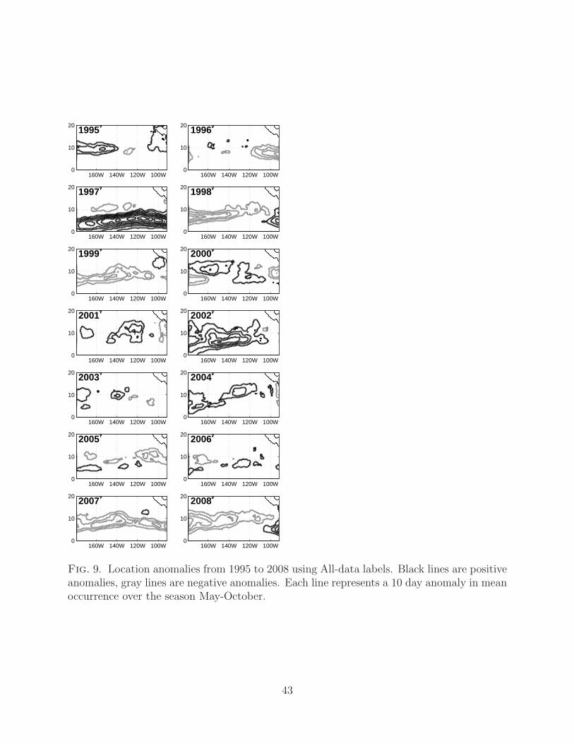
b. Interannual variability

The All-data labels were used to examine interannual variability in location, shown in

Fig. 9. The plots are anomalies from the mean location of ITCZ (Fig. 5(a)). The figure

shows considerable variability in the location of the ITCZ from year to year and especially

demonstrates the strong influence of El Nino. Particularly noticeable are the El Nino events

in 1997 and 2002 when the ITCZ region increased both in size and frequency of occurrence.

The El Nino in 1997 was particularly notable for the large average area of ITCZ – this was

also a strong El Nino event (McPhaden 1999). The La Nina events were in 1995 (weak),

1998, 2000 and 2008. In general, the ITCZ during La Nina is smaller than average in area,

although that was not the case in 2000.

The IR-only labels were used to investigate climatic trends in the ITCZ from 1980 to 2009.

The IR satellite record had some data gaps in the early 1980s and although the statistical

model is able to handle gaps in data, diagnosis is less reliable if data are not available for

several sequential time steps. Therefore IR images where greater than 20% of the image

was missing were removed unless the images on each side in time were more complete. This

led to less information going into the data series in 1980-1991 where on average 2 days per

month were missing or incomplete in the satellite record.

Figure 9 was reproduced using IR-only labels to examine location trends from 1980-2009.

As mentioned at the beginning of the Section, the area of the ITCZ was reduced in the 120-

150W region due to lower cloud not being identified in the IR. Again, there were positive

anomalies in location in El Nino years and mostly negative in La Nina years. However,

the figure is qualitatively similar to Fig. 9. Linear regression was performed to remove the

20

influence of ENSO (in a similar manner to Vimont et al. 2001) on the mean annual ITCZ

location so that climatic trends could be studied. The years where the multivariate ENSO

index (Wolter and Timlin 1998) was greater than 0.5 were selected and the anomalies from

mean location combined and weighted by ENSO index to produce a composite picture of

typical El Nino year ITCZ location anomaly. This typical composite could then be removed

from the El Nino years (weighted by the strength of ENSO). The same was performed for La

Nina years where ENSO index was less than -0.5. By this means, the influence of ENSO was

removed or reduced, and any climatic shifts in the the location of the ITCZ not due to ENSO

should be revealed. Several analyses were done on the resulting data and no significant or

consistent trends in location were found. However, there is much variability from year to

year even after removal of the ENSO signature.

In addition to this analysis, histograms of latitudinal distribution each year were inves-

tigated and again, no climatic shifts in the position of the ITCZ could be detected. This

suggests that any trends in ITCZ location over the 30 years (that are not due to ENSO),

are quite small or non-existent.

Figure 10a shows the mean area of ITCZ from the IR-only labels for May to October

each year, alongside the ENSO index. It should be noted that the time axis (x-axis) is

not continuous. Only the months of May through October are depicted each year. The

plot shows high correlation between the ENSO index and the area covered by ITCZ. The

correlation coefficient is 0.67, confirming the influence of ENSO in determining ITCZ area.

To determine the long term trends in the area of ITCZ independent of ENSO, the ITCZ data

were normalized to vary between 0 and 1 and the normalized ENSO index was removed. The

resulting time series is shown in Fig. 10b. The plot shows that there is no overall trend in

21

ITCZ area over the 30 years but there is much variability in size from one year to the next.

6. Concluding remarks

Our method has identified the ITCZ as a distinct weather feature in the east Pacific in

instantaneous satellite data. The data set has revealed the seasonal evolution of the ITCZ

in the east Pacific and its interannual variability. The location and area of the ITCZ varies

significantly on interannual timescales and is highly correlated with the ENSO index. During

El Nino years there were significant shifts in ITCZ location in tandem with shifts in ocean

warm-pool regions and the average area of the ITCZ was greater than in ENSO-neutral

years. Inspection of the 30 year ITCZ data set using IR-only labels, showed no consistent

trend in the area covered by ITCZ or shifts in ITCZ location when the influence of ENSO

was removed.

The ITCZ climatology of Waliser and Gautier (1993) which used cold cloud thresholding

of the seasonal average to determine the signature of the mean convergence zone, described

the ITCZ in the Pacific in a general sense. The mean latitude location was given as 8◦ N.

This is in general agreement with our results, but moreover our results show the seasonal

migration of the ITCZ and significant interannual variability. The ITCZ location is closely

associated with SST. In the mean fields, the far eastern Pacific ITCZ is located to the south

of the maximum SSTs, whereas in the central Pacific (150-180◦W), the ITCZ is located to

the north of the maximum SSTs.

Our results show that there is a westward shift in ITCZ location throughout boreal

summertime. The ITCZ is more concentrated in the east Pacific in May to July, and more

22

distributed to the central Pacific in September and October. The ITCZ area in the east

Pacific peaks in late June and late August. The secondary maximum could be due to an

increase in the number of tropical cyclones and other WPDs in August.

The application of statistical techniques in identifying the ITCZ has been shown to be

successful. The labels automatically generated from the statistical model present a time-

saving alternative to manual labelling. The model allows vast quantities of data to be

analysed for the presence of meteorological features at relatively little computational cost.

The model uses fast, portable code which can be run on any desktop: to identify the ITCZ

for 6 months of 3-hourly data takes approximately 20 minutes on a parallelized computer

using 8 processors.

The use of the statistical model is ideal for this particular weather feature due to the

ITCZ’s persistent nature (rendering the use of the time component in the Markov random

field highly appropriate), and the need to discard unrelated cloud features in the satellite

images. Validation against manual labellers found that the statistical model was better

equipped to identify coherent structures than thresholding techniques. Furthermore, thresh-

olding of IR will not include low-cloud signatures in the ITCZ that are important for climate

studies (Clement et al. 2009).The primary advantage of the MRF approach over other tech-

niques is its accuracy in determining the ITCZ envelope. The model is able to take expert

opinion, in the form of manual labels, and systematize the evaluation of the phenomenon

over a long time period.

Here we have presented the seasonal and interannual characteristics of the ITCZ, but

other uses of the data take advantage of the high temporal sampling of the new ITCZ

labels (e.g. Bain et al. 2010). The three hourly timescale available in this data set will

23

allow investigations of internal ITCZ dynamical interactions as well as ITCZ relationships

to different tropical features from the Madden-Julian Oscillation to Kelvin waves. Future

work could also experiment to improve the model, perhaps using different neighborhood

structures, adding a time dimension to the location prior, or clarifying the impact of altering

the strength of the β’s. With the success of the method there is also the possibility of

applying the technique to the detection of the ITCZ in other regions of the world. The

model is thus far trained on manual labels of the ITCZ in the Pacific region but has the

potential to be retrained for other global locations if manual labelling is carried out. Post

processing can be tailored to the needs of any user. Another future research possibility

is to apply this MRF approach to tracking non-ITCZ features such as weather systems in

the extra-tropical storm tracks. It also has the potential to be used in other fields such as

oceanography to track ocean eddies or phytoplankton blooms.

Acknowledgments.

The authors would like to acknowledge Ken Knapp at NOAA’s National Climatic Data

Center for providing all IR and VS data from the HURSAT-Basin archive. We would also

like to thank Deborah Smith at Remote Sensing Systems for providing the TPW data from

combined radar satellite instruments. We thank Mark DeMaria for valuable comments during

this research and Yi-Hui Wang for help help with labeling data. This research was supported

by NSF Grant ATM0530926 and NOAA Grant NA09OAR4310132.

24

APPENDIX A

Identification of tropical cyclones

Tropical cyclones produce large cloud signatures that can be embedded or isolated from

the main cloudy region of the ITCZ. It is therefore of interest to know what parts of the

ITCZ labels may be associated with tropical cyclones.

The horizontal extent of tropical cyclones is most often distinguished by regions of sus-

tained wind speed over 17 m s−1, e.g. as specified by the National Hurricane Center4.

However, higher wind speeds do not necessarily equate to the full extent of the cloud cover

associated with the cyclone, and wind speeds are often only above tropical storm speed

within a few degrees of the center of the eye. Therefore a second algorithm using the same

IR satellite data as our statistical model was applied to identify the clouds belonging to

tropical cyclones. Best track data from the HURDAT data set1 was used to establish the

location of the eye of the storm. The data was linearly interpolated from the 6 hourly data

set to every 3 hours. High clouds (< 255 K) overlapping a 9 grid point neighborhood near the

eye were selected, along with any intersecting low cloud (< 270 K), but not non-intersecting

high cloud. In this way if a cyclone was embedded in the ITCZ, the cloud belonging to the

cyclone (only) was distinguished. A maximum radius was defined as 400 km, but this was

rarely reached by the algorithm.

This method was seen as a balance between using more complex methods of pattern

4www.nhc.noaa.gov

25

recognition and simpler methods such as defining a generic circle around all cyclone eyes

as tropical cyclone cloud. The algorithm was able to adapt when cyclone-associated cloud

was unusually positioned, or the cyclone was embedded within a larger cloudy region. The

inferred cyclone data is used in Section 5a, and may be used for future investigations on

interactions between cyclones and the ITCZ.

26

REFERENCES

Bain, C. L., G. Magnusdottir, P. Smyth, and H. Stern, 2010: The Diurnal Cycle of the ITCZ

in the East Pacific. J. Geophys. Res., submitted.

Clement, A., R. Burgerman, and J. Norris, 2009: Observational and model evidence for

positive low-level cloud feedback. Science, 325, 460–464.

Ferreira, R. N. and W. H. Schubert, 1997a: Barotropic aspects of itcz breakdown. J. Atmos.

Sci., 54, 261–285.

Ferreira, R. N. and W. H. Schubert, 1997b: Barotropic aspects of ITCZ breakdown. J.

Atmos. Sci., 54, 261–285.

Garcia, O., 1985: Atlas of highly reflective clouds for the global tropics: 1971-1983. U.S.

Dept. of Commerce, NOAA, Environmental Research Lab., Boulder, CO, 365, [NTIS PB-

87129169.].

Gelman, A., J. B. Carlin, H. S. Stern, and D. B. Rubin, 2003: Bayesian Data Analysis.

Chapman and Hall/CRC: Boca Raton.

Geman, S. and D. Geman, 1984: Stochastic relaxation, Gibbs distribution and the Bayesian

restoration of images. IEEE Transaction on Pattern Analysis and Machine Intelligence,

6, 721–741.

27

Gilks, W., S. Richardson, and D. Spiegelhalter, 1993: Markov Chain Monte Carlo in Practice.

Chapman and Hall/CRC: Boca Raton.

Gu, G. and C. Zhang, 2002a: Cloud components of the ITCZ. J. Geophys. Res., 107, 4565,

dOI:10.1029/2002JD002089.

Gu, G. and C. Zhang, 2002b: Westward-propagating synoptic-scale disturbances and the

ITCZ. J. Atmos. Sci., 59, 1062–1075.

Kindermann, R. and J. L. Snell, 1980: Markov random fields and their application. American

Mathematical Society: Providence, RI.

Knapp, K. R., 2008: Calibration assessment of ISCCP geostationary infrared observations

using HIRS. Journal of Atmos. and Ocean Tech., 25, 183–195.

Knapp, K. R. and J. P. Kossin, 2007: New global tropical cyclone data from ISCCP B1

geostationary satellite observations. J. App. Remote Sensing, 1, 013 505.

Li, S. Z., 1994: Markov Random Field Models in Computer Vision. Lecture Notes in Com-

puter Science. Springer: Heidelberg.

Magnusdottir, G. and Wang, 2008: Intertropical convergence zones during the active season

in daily data. J. Atmos. Sci., 65, 2425–2436.

McPhaden, M. J., 1999: Genesis and evolution of the 1997-98 El Nino. Science, 283, 950–

954.

Mitchell, T. P. and J. M. Wallace, 1992: The annual cycle in equatorial convection and sea

surface temperature. J. Climate, 5, 1140–1156.

28

Raymond, D. J., C. S. Bretherton, and J. Molinari, 2006: Dynamics of the Intertropical

convergence zone of the east Pacific. J. Atmos. Sci., 63, 582–597.

Raymond, D. J., G. B. Raga, C. S. Bretherton, J. Molinari, C. Lopez-Carrillo, and Z. Fuchs,

2003: Convective forcing in the Intertropical convergence zone of the eastern Pacific. J.

Atmos. Sci., 60, 2064–2082.

Scharenbroich, L., G. Magnusdottir, P. Smyth, H. Stern, and C.-C. Wang, 2010: A Bayesian

framework for storm tracking using a hidden state representation. Mon. Weather Rev.

Serra, Y. and R. A. Houze, 2002: Observations of variability on synoptic timescales in the

east Pacific ITCZ. J. Atmos. Sci., 59, 1723–1743.

Smyth, P., 1997: Belief networks, hidden Markov models, and Markov random fields: A

unified view. Pattern Recognition Letters, 18, 1261–1268.

Thorncroft, C. and K. Hodges, 2001: African easterly wave variability and its relationship

to Atlantic tropical cyclone activity. J. Climate, 14, 1166–1179.

Vimont, D. J., D. S. Battisti, and A. C. Hirst, 2001: Footprinting: A seasonal connection

between the tropics and mid-latitudes. Geophys. Res. Lett., 28, 3923–3926.

Waliser, D. E. and C. Gautier, 1993: A satellite-derved climatology of the ITCZ. J. Climate,

6, 2162–2174.

Wang, C.-C., C. Chou, and W.-L. Lee, 2010: Breakdown and reformation of the Intertropical

convergence zone in a moist atmosphere. J. Atmos. Sci., 67, 1247–1260.

29

Wang, C.-C. and G. Magnusdottir, 2005: ITCZ breakdown in the three-dimensional flows.

J. Atmos. Sci., 62, 1497–1512.

Wang, C.-C. and G. Magnusdottir, 2006: The ITCZ in the central and eastern Pacific on

synoptic time scales. Mon. Weather Rev., 134, 1405–1421.

Wolter, K. and M. S. Timlin, 1998: Measuring the strength of ENSO events - how does

1997/98 rank? Weather, 53, 315–324.

Zhang, C., M. McGauley, and N. A. Bond, 2004: Shallow meridional circulation in the

tropical Eastern Pacific. J. Climate, 17, 133–139.

30

List of Tables

1 Table showing the comparisons between a union of the manual labels defined

as ITCZ and each method of detection for August 2000. False negative is

the number of ITCZ grid points not detected by each method divided by

the number of ITCZ grid points. False positive is the number of grid points

incorrectly detected as ITCZ by each method divided by the number of ITCZ

grid points in the union. Results given as percentages where low numbers

indicate better agreement between methods, accept for the final column where

a higher number indicates better agreement. See text for more details. 32

31

Table 1. Table showing the comparisons between a union of the manual labels defined asITCZ and each method of detection for August 2000. False negative is the number of ITCZgrid points not detected by each method divided by the number of ITCZ grid points. Falsepositive is the number of grid points incorrectly detected as ITCZ by each method dividedby the number of ITCZ grid points in the union. Results given as percentages where lownumbers indicate better agreement between methods, accept for the final column where ahigher number indicates better agreement. See text for more details.

Method tested Base method testedagainst

Falsenegative

Falsepositive

Totalabsoluteerror

intersection/union

Person P1 Union P2, P3 5.9 2.3 8.2 57.9Person P2 Union P1, P3 7.2 2.8 10.1 51.4Person P3 Union P1, P2 7.7 2.2 9.9 49.3

All-data labels Union P1, P2, P3 7.5 4.4 11.9 49.2IR-only labels 11.3 2.6 13.9 37.9Threshold IR 12.3 3.7 16.0 32.6Threshold TPW 6.7 9.8 16.4 43.4If all domain ’ITCZ’ 0.0 78.8 78.8 21.2If all domain ’non-ITCZ’ 21.2 0.0 21.2 0.0

All-data labels Threshold IR 1.9 7.3 9.2 53.5IR-only labels 2.2 2.0 4.2 67.5Threshold TPW 2.7 14.3 17.0 35.4If all domain ITCZ 0.0 87.3 87.3 12.7If all domain non-ITCZ 12.7 0.0 12.7 0.0

All-data labels Threshold TPW 8.2 1.9 10.0 57.3IR-only labels 13.9 2.0 15.9 36.6Threshold IR 14.3 2.7 17.0 35.4If all domain ITCZ 0 75.6 75.6 24.4If all domain non-ITCZ 24.4 0 24.4 0

32

List of Figures

1 Schematic of the neighborhood structure used in the MRF. X is the status

of ITCZ or non-ITCZ at grid point i, j, t. Y is the satellite data, and q is the

spatial prior value at the grid point. The binary status of Xi,j,t depends on

Yi,j,t, the status of X in the neighboring grid points in space and time, and qj. 35

2 (a) Map of the study region (black rectangle) split into 3 longitudinal boxes

in gray (used in Section 5). (b) Spatial prior for the model for All-data labels

(solid) and IR-only labels (dashed) as a function of latitude. The spatial prior

gives a starting point for the probability that grid point locations are part of

the ITCZ. Each spatial prior is zonally uniform across the domain. 36

3 ITCZ label for 19 August 2000 at 2100 UTC overlaid on the IR image: (a)

Manual label (union of 3 labellers), (b) Statistical model using IR, VS and

TPW satellite data, (c) Threshold at 270K (without post-processing). Shad-

ing represents the IR image with the temperature scale provided below. The

bold contours mark the ITCZ labels 37

4 Schematic showing the areas that are used to assess the agreement between

ITCZ labels found using different methods. The outline of the ITCZ is shown

by the solid curve for the base method and by the dashed curve for the test

method. 38

5 Fraction of time when ITCZ is present during May-October from 1995-2008

with (a) All-data labels, (b) IR-only labels. (c) Mean IR is shown for com-

parison, where cold temperatures indicate higher cloud tops. 39

33

6 (a) Mean width of ITCZ for (shaded) in degrees latitude versus time of year

using All-data labels (1995-2008). (b) Mean area of cloud (km2)associated

with tropical cyclones versus time of year from 1995-2008. 40

7 (a) Mean SST (shaded) with mean ITCZ days per season contoured every

20 days. (b-g) Monthly anomalies of ITCZ location (contoured) overlaid on

monthly anomalies of SST. All averaged from 1995-2008. The contours repre-

sent median number of days in the month when ITCZ is present in comparison

to the mean, part (a). Black curves are positive anomalies, gray curves are

negative anomalies. The contour interval for the anomalies is 2 days. SST is

in Celsius as shown in the color bars. 41

8 Median latitude of ITCZ distribution in two longitudinal box regions: 90-

120◦W (bold curve) and 150-180◦W (dashed curve). Standard deviation is

shown in the shading. 42

9 Location anomalies from 1995 to 2008 using All-data labels. Black lines are

positive anomalies, gray lines are negative anomalies. Each line represents a

10 day anomaly in mean occurrence over the season May-October. 43

10 (a) Mean area of ITCZ labels in black (monthly means May to October) shown

alongside ENSO index for the same months. (b) Area of mean annual ITCZ

normalized with normalized ENSO index removed. 44

34

X i,j+1,t

i+1,j,tXX i−1,j,t

X i,j−1,t

X i,j,t+1

satellite data

Yi,j,t

LONGITUDE, i

LAT

ITU

DE

, j

TIME, t

image t+1

image t

image t−1jq

Xi,j,t

X i,j,t−1

Fig. 1. Schematic of the neighborhood structure used in the MRF. X is the status of ITCZor non-ITCZ at grid point i, j, t. Y is the satellite data, and q is the spatial prior value at thegrid point. The binary status of Xi,j,t depends on Yi,j,t, the status of X in the neighboringgrid points in space and time, and qj.

35

0 0.2 0.4−10

0

10

20

30

40

50

prior strength

LAT

ITU

DE

(b)All−data

IR−only

150E 180E 150W 120W 90W−10

0

10

20

30

40

50

LONGITUDE

LAT

ITU

DE

(a)

Fig. 2. (a) Map of the study region (black rectangle) split into 3 longitudinal boxes ingray (used in Section 5). (b) Spatial prior for the model for All-data labels (solid) andIR-only labels (dashed) as a function of latitude. The spatial prior gives a starting point forthe probability that grid point locations are part of the ITCZ. Each spatial prior is zonallyuniform across the domain.

36

LAT

ITU

DE

(a) Manual label

180W 160W 140W 120W 100W0

5

10

15

20

25

LAT

ITU

DE

(b) Statisical model (All−data)

180W 160W 140W 120W 100W0

5

10

15

20

25

LAT

ITU

DE

(c) Threshold at 270K

IR Temperature (K)

180W 160W 140W 120W 100W0

5

10

15

20

25

210 220 230 240 250 260 270 280 290 300 310

Fig. 3. ITCZ label for 19 August 2000 at 2100 UTC overlaid on the IR image: (a) Manuallabel (union of 3 labellers), (b) Statistical model using IR, VS and TPW satellite data, (c)Threshold at 270K (without post-processing). Shading represents the IR image with thetemperature scale provided below. The bold contours mark the ITCZ labels

37

BC A

base method test method

Dlimit of domain

Fig. 4. Schematic showing the areas that are used to assess the agreement between ITCZlabels found using different methods. The outline of the ITCZ is shown by the solid curvefor the base method and by the dashed curve for the test method.

38

Fig. 5. Fraction of time when ITCZ is present during May-October from 1995-2008 with(a) All-data labels, (b) IR-only labels. (c) Mean IR is shown for comparison, where coldtemperatures indicate higher cloud tops.

39

0 2 4 6

x 105

Jun

Jul

Aug

Sep

Oct

(b) Area TC cloud

May

(a) Width of the ITCZ (degrees Latitude)

May180W 160W 140W 120W 100W

Jun

Jul

Aug

Sep

Oct

1 2 3 4 5 6 7

Fig. 6. (a) Mean width of ITCZ for (shaded) in degrees latitude versus time of year usingAll-data labels (1995-2008). (b) Mean area of cloud (km2)associated with tropical cyclonesversus time of year from 1995-2008.

40

1

11 11 3

355 7

−7−7−7−5

−5

−5

−5−3

−3

−3

−3

−1

−1

−1−1

(b) MAY

180W 160W 140W 120W 100W0

5

10

15

20

−1.5

−0.5

0.5

1.5

11

1

11

1 3 5

−5 −5−5−5−3

−3

−1

−1

−1

(c) JUN

180W 160W 140W 120W 100W0

5

10

15

20

−1.5

−0.5

0.5

1.5

1

11

1

1

1

3

333

3

3

35−1

−1

(d) JUL

180W 160W 140W 120W 100W0

5

10

15

20

−1.5

−0.5

0.5

1.5

1

11

1

1

1

3

333 3

3

3 33

55

555 7

−3−1

−1−1

(e) AUG

180W 160W 140W 120W 100W0

5

10

15

20

−1.5

−0.5

0.5

1.5

1

1

1

1

1

11 33

35

−5−3−3−3−3−1

−1

−1−1

(f) SEP

180W 160W 140W 120W 100W0

5

10

15

20

−1.5

−0.5

0.5

1.5

1

1

13

355 7

−7−5−5−3

−1

−1

−1−1

−1

−1

−1−1(g) OCT

180W 160W 140W 120W 100W0

5

10

15

20

−1.5

−0.5

0.5

1.5

(a) Mean SST and mean ITCZ

180W 160W 140W 120W 100W0

5

10

15

20

24

26

28

29.5

Fig. 7. (a) Mean SST (shaded) with mean ITCZ days per season contoured every 20 days.(b-g) Monthly anomalies of ITCZ location (contoured) overlaid on monthly anomalies ofSST. All averaged from 1995-2008. The contours represent median number of days in themonth when ITCZ is present in comparison to the mean, part (a). Black curves are positiveanomalies, gray curves are negative anomalies. The contour interval for the anomalies is 2days. SST is in Celsius as shown in the color bars.

41

Fig. 8. Median latitude of ITCZ distribution in two longitudinal box regions: 90-120◦W(bold curve) and 150-180◦W (dashed curve). Standard deviation is shown in the shading.

42

1995

160W 140W 120W 100W0

10

201996

160W 140W 120W 100W0

10

20

1997

160W 140W 120W 100W0

10

201998

160W 140W 120W 100W0

10

20

1999

160W 140W 120W 100W0

10

202000

160W 140W 120W 100W0

10

20

2001

160W 140W 120W 100W0

10

202002

160W 140W 120W 100W0

10

20

2003

160W 140W 120W 100W0

10

202004

160W 140W 120W 100W0

10

20

2005

160W 140W 120W 100W0

10

202006

160W 140W 120W 100W0

10

20

2007

160W 140W 120W 100W0

10

202008

160W 140W 120W 100W0

10

20

Fig. 9. Location anomalies from 1995 to 2008 using All-data labels. Black lines are positiveanomalies, gray lines are negative anomalies. Each line represents a 10 day anomaly in meanoccurrence over the season May-October.

43

1980 1982 1984 1986 1988 1990 1992 1994 1996 1998 2000 2002 2004 2006 2008 20100

2

4

6

Are

a of

ITC

Z (

×106 k

m2 )

year1980 1982 1984 1986 1988 1990 1992 1994 1996 1998 2000 2002 2004 2006 2008 2010

−2

0

2

4

EN

SO

inde

x

(a)

1980 1982 1984 1986 1988 1990 1992 1994 1996 1998 2000 2002 2004 2006 2008 2010

−0.2

−0.1

0

0.1

0.2

year

norm

aliz

ed IT

CZ

are

aw

ith E

NS

O r

emov

ed

(b)

Fig. 10. (a) Mean area of ITCZ labels in black (monthly means May to October) shownalongside ENSO index for the same months. (b) Area of mean annual ITCZ normalized withnormalized ENSO index removed.

44