Light-time computations for the BepiColombo

Radio Science Experiment

G. Tommei1, A. Milani1 and D. Vokrouhlicky2

1 Department of Mathematics, University of Pisa,Largo B. Pontecorvo 5, 56127 Pisa, Italy

e-mail: tommei@dm.unipi.it, milani@dm.unipi.it2 Institute of Astronomy, Charles University,

V Holesovickach 2, CZ-18000 Prague 8, Czech Republice-mail: vokrouhl@cesnet.cz

Abstract

The Radio Science Experiment is one of the on board experiments ofthe Mercury ESA mission BepiColombo that will be launched in 2014.The goals of the experiment are to determine the gravity field of Mer-cury and its rotation state, to determine the orbit of Mercury, to con-strain the possible theories of gravitation (for example by determiningthe post-Newtonian (PN) parameters), to provide the spacecraft positionfor geodesy experiments and to contribute to planetary ephemerides im-provement. This is possible thanks to a new technology which allows toreach great accuracies in the observables range and range rate; it is wellknown that a similar level of accuracy requires studying a suitable modeltaking into account numerous relativistic effects. In this paper we dealwith the modelling of the space-time coordinate transformations neededfor the light-time computations and the numerical methods adopted toavoid rounding-off errors in such computations.

Keywords: Mercury, Interplanetary tracking, Light-time, Relativistic effects,Numerical methods

1 Introduction

BepiColombo is an European Space Agency mission to be launched in 2014,with the goal of an in-depth exploration of the planet Mercury; it has beenidentified as one of the most challenging long-term planetary projects. Onlytwo NASA missions had Mercury as target in the past, the Mariner 10, whichflew by three times in 1974-5 and Messenger, which carried out its flybys onJanuary and October 2008, September 2009 before it starts its year-long orbiterphase in March 2011.

1

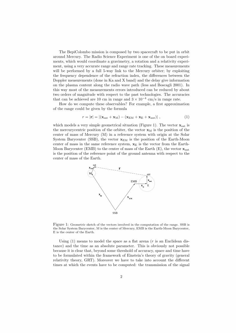
The BepiColombo mission is composed by two spacecraft to be put in orbitaround Mercury. The Radio Science Experiment is one of the on board experi-ments, which would coordinate a gravimetry, a rotation and a relativity experi-ment, using a very accurate range and range rate tracking. These measurementswill be performed by a full 5-way link to the Mercury orbiter; by exploitingthe frequency dependence of the refraction index, the differences between theDoppler measurements (done in Ka and X band) and the delay give informationon the plasma content along the radio wave path (Iess and Boscagli 2001). Inthis way most of the measurements errors introduced can be reduced by abouttwo orders of magnitude with respect to the past technologies. The accuraciesthat can be achieved are 10 cm in range and 3 × 10−4 cm/s in range rate.

How do we compute these observables? For example, a first approximationof the range could be given by the formula

r = |r| = |(xsat + xM) − (xEM + xE + xant)| , (1)

which models a very simple geometrical situation (Figure 1). The vector xsat isthe mercurycentric position of the orbiter, the vector xM is the position of thecenter of mass of Mercury (M) in a reference system with origin at the SolarSystem Barycenter (SSB), the vector xEM is the position of the Earth-Mooncenter of mass in the same reference system, xE is the vector from the Earth-Moon Barycenter (EMB) to the center of mass of the Earth (E), the vector xant

is the position of the reference point of the ground antenna with respect to thecenter of mass of the Earth.

r

xM x

xant

xE

xsat

EM

SSB

M ant

sat

EMB

E

Figure 1: Geometric sketch of the vectors involved in the computation of the range. SSB isthe Solar System Barycenter, M is the center of Mercury, EMB is the Earth-Moon Barycenter,E is the center of the Earth.

Using (1) means to model the space as a flat arena (r is an Euclidean dis-tance) and the time as an absolute parameter. This is obviously not possiblebecause it is clear that, beyond some threshold of accuracy, space and time haveto be formulated within the framework of Einstein’s theory of gravity (generalrelativity theory, GRT). Moreover we have to take into account the differenttimes at which the events have to be computed: the transmission of the signal

2

at the transmit time (tt), the signal at the Mercury orbiter at the time of bounce(tb) and the reception of the signal at the receive time (tr).

Formula (1) is used as a starting point to construct a correct relativisticformulation; with the word “correct” we do not mean all the possible relativisticeffects, but the effects that can be measured by the experiment. This paper dealswith the corrections to apply to this formula to obtain a consistent relativisticmodel for the computations of the observables and the practical implementationof such computations.

In Section 2 we discuss the relativistic four-dimensional reference systemsused and the transformations adopted to make the sums in (1) consistent; ac-cording to (Soffel et al. 2003), with “reference system” we mean a purely math-ematical construction, while a “reference frame” is a some physical realizationof a reference system. The relativistic contribution to the time delay due to theSun’s gravitational field, the Shapiro effect, is described in Section 3. Section 4deals with the theoretical procedure to compute the light-time (range) and theDoppler shift (range rate). In Section 5 we discuss the practical implementationof the algorithms showing how we solve the rounding-off problems.

The equations of motion for the planets Mercury and Earth, including all therelativistic effects (and potential violations of GRT) required to the accuracyof the BepiColombo Radio Science Experiment have already been discussed in(Milani et al. 2010), thus this paper focuses on the computation of the observ-ables.

2 Space-time reference frames and transforma-

tions

The five vectors involved in formula (1) have to be computed at their owntime, the epoch of different events: e.g., xant, xEM and xE are computed atboth the antenna transmit time tt and receive time tr of the signal. xM andxsat are computed at the bounce time tb (when the signal has arrived to theorbiter and is sent back, with correction for the delay of the transponder). Inorder to be able to perform the vector sums and differences, these vectors haveto be converted to a common space-time reference system, the only possiblechoice being some realization of the BCRS (Barycentric Celestial ReferenceSystem). We adopt for now a realization of the BCRS that we call SSB (SolarSystem Barycentric) reference frame and in which the time is a re-definition ofthe TDB (Barycentric Dynamic Time), according to the IAU 2006 ResolutionB31; other possible choices, such as TCB (Barycentric Coordinate Time), onlycan differ by linear scaling. The TDB choice of the SSB time scale entailsalso the appropriate linear scaling of space-coordinates and planetary masses asdescribed for instance in (Klioner 2008) or (Klioner et al. 2010).

The vectors xM, xE, and xEM are already in SSB as provided by numericalintegration and external ephemerides; thus the vectors xant and xsat have to

1See the Resolution at http://www.iau.org/administration/resolutions/ga2006/

3

be converted to SSB from the geocentric and mercurycentric systems, respec-tively. Of course the conversion of reference system implies also the conversionof the time coordinate. There are three different time coordinates to be con-sidered. The currently published planetary ephemerides are provided in TDB.The observations are based on averages of clock and frequency measurements onthe Earth surface: this defines another time coordinate called TT (TerrestrialTime). Thus for each observation the times of transmission tt and receptiontr need to be converted from TT to TDB to find the corresponding positionsof the planets, e.g., the Earth and the Moon, by combining information fromthe pre-computed ephemerides and the output of the numerical integration forMercury and for the Earth-Moon barycenter. This time conversion step is nec-essary for the accurate processing of each set of interplanetary tracking data;the main term in the difference TT-TDB is periodic, with period 1 year andamplitude ≃ 1.6 × 10−3 s, while there is essentially no linear trend, as a resultof a suitable definition of the TDB.

The equation of motion of a mercurycentric orbiter can be approximated, tothe required level of accuracy, by a Newtonian equation provided the indepen-dent variable is the proper time of Mercury. Thus, for the BepiColombo RadioScience Experiment, it is necessary to define a new time coordinate TDM (Mer-cury Dynamic Time), as described in (Milani et al. 2010), containing terms of1-PN order depending mostly upon the distance from the Sun and velocity ofMercury.

From now on, in accordance with (Klioner et al. 2010), we shall call thequantities related to the SSB frame “TDB-compatible”, the quantities relatedto the geocentric frame “TT-compatible”, the quantities related to the mer-curycentric frame “TDM-compatible” and label them TB, TT and TM, respec-tively.

The differential equation giving the local time T as a function of the SSBtime t , which we are currently assuming to be TDB, is the following:

dT

dt= 1 −

1

c2

[

U +v2

2− L

]

, (2)

where U is the gravitational potential (the list of contributing bodies dependsupon the accuracy required: in our implementation we use Sun, Mercury to Nep-tune, Moon) at the planet center and v is the SSB velocity of the same planet.The constant term L is used to perform the conventional rescaling motivatedby removal of secular terms, e.g., for the Earth we use LC (Soffel et al. 2003).

The space-time transformations to perform involve essentially the positionof the antenna and the position of the orbiter. The geocentric coordinatesof the antenna should be transformed into TDB-compatible coordinates; thetransformation is expressed by the formula

xTBant = xTT

ant

(

1 −U

c2− LC

)

−1

2

(

vTBE · xTT

ant

c2

)

vTBE ,

where U is the gravitational potential at the geocenter (excluding the Earthmass), LC = 1.48082686741 × 10−8 is a scaling factor given as definition, sup-

4

posed to be a good approximation for removing secular terms from the trans-formation and vTB

E is the barycentric velocity of the Earth. The next formulacontains the effect on the velocities of the time coordinate change, which shouldbe consistently used together with the coordinate change:

vTBant =

[

vTTant

(

1 −U

c2− LC

)

−1

2

(

vTBE · vTT

ant

c2

)

vTBE

] [

dT

dt

]

.

Note that the previous formula contains the factor dT/dt (expressed by (2))that deals with a time transformation: T is the local time for Earth, that is TT,and t is the corresponding TDB time.

The mercurycentric coordinates of the orbiter have to be transformed intoTDB-compatible coordinates through the formula

xTBsat = xTM

sat

(

1 −U

c2− LCM

)

−1

2

(

vTBM · xTM

sat

c2

)

vTBM ,

where U is the gravitational potential at the center of mass of Mercury (exclud-ing the Mercury mass) and LCM could be used to remove the secular term in thetime transformation (thus defining a TM scale, implying a rescaling of the massof Mercury). We believe this is not necessary: the secular drift of TDM with re-spect to other time scales is significant, see Figure 5 in (Milani et al. 2010), but asimple iterative scheme is very efficient in providing the inverse time transforma-tion. Thus we set LCM = 0, assuming the reference frame is TDM-compatible.As for the antenna we have a formula expressing the velocity transformationthat contains the derivative of time T for Mercury, that is TDM, with respectto time t, that is TDB:

vTBsat =

[

vTMsat

(

1 −U

c2− LCM

)

−1

2

(

vTBM · vTM

sat

c2

)

vTBM

] [

dT

dt

]

.

For these coordinate changes, in every formula we neglected the terms of the SSBacceleration of the planet center (Damour et al. 1994), because they containbeside 1/c2 the additional small parameter (distance from planet center)/(planetdistance to the Sun), which is of the order of 10−4 even for a Mercury orbiter.

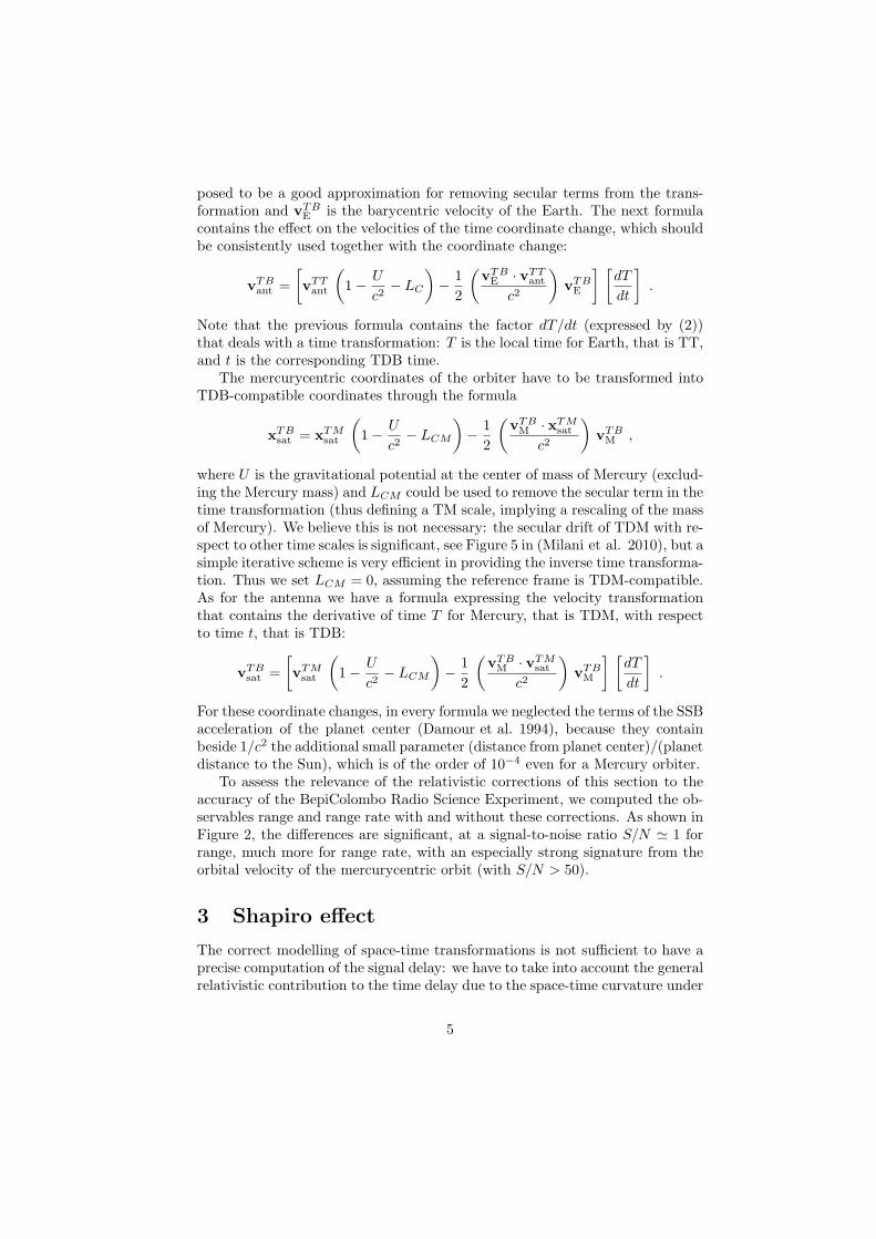
To assess the relevance of the relativistic corrections of this section to theaccuracy of the BepiColombo Radio Science Experiment, we computed the ob-servables range and range rate with and without these corrections. As shown inFigure 2, the differences are significant, at a signal-to-noise ratio S/N ≃ 1 forrange, much more for range rate, with an especially strong signature from theorbital velocity of the mercurycentric orbit (with S/N > 50).

3 Shapiro effect

The correct modelling of space-time transformations is not sufficient to have aprecise computation of the signal delay: we have to take into account the generalrelativistic contribution to the time delay due to the space-time curvature under

5

0 0.05 0.1 0.15 0.2 0.25 0.3 0.35 0.4 0.45−10

−5

0

5Change in the observable

time, days from arc beginning

Ran

ge, c

m

0 0.05 0.1 0.15 0.2 0.25 0.3 0.35 0.4 0.45−0.02

−0.01

0

0.01

0.02

time, days from arc beginning

Ran

ge−

rate

, cm

/s

0 0.05 0.1 0.15 0.2 0.25 0.3 0.35 0.4 0.45−16

−14

−12

−10

−8

−6

−4Change in the observable

time, days from arc beginning

Ran

ge, c

m

0 0.05 0.1 0.15 0.2 0.25 0.3 0.35 0.4 0.45−1.5

−1

−0.5

0

0.5

1

1.5

2x 10

−3

time, days from arc beginning

Ran

ge−

rate

, cm

/s

Figure 2: The difference in the observables range and range rate for one pass of Mercuryabove the horizon for a ground station, by using an hybrid model in which the position andvelocity of the orbiter have not transformed to TDB-compatible quantities and a correct modelin which all quantities are TDB-compatible. Interruptions of the signal are due to spacecraftpassage behind Mercury as seen for the Earth station. Top: for an hybrid model with thesatellite position and velocity not transformed to TDB-compatible. Bottom: for an hybridmodel with the position and velocity of the antenna not transformed to TDB-compatible.

the effect of the Sun’s gravitational field, the Shapiro effect (Shapiro 1964).The Shapiro time delay ∆t at the 1-PN level, according to (Will 1993) and(Moyer 2003), is

∆t =(1 + γ)µ0

c3ln

(

rt + rr + r

rt + rr − r

)

, S(γ) = c∆t

where rt = |rt| and rr = |rr| are the heliocentric distances of the transmitterand the receiver at the corresponding time instants of photon transmission andreception, µ0 is the gravitational mass of the Sun (µ0 = Gm0) and r = |rr −rt|.The planetary terms, similar to the solar one, can also be included but theyare smaller than the accuracy needed for our measurements. Parameter γ isthe only post-Newtonian parameter used for the light-time effect and, in fact,it could be best constrained during superior conjunction (Milani et al. 2002).

6

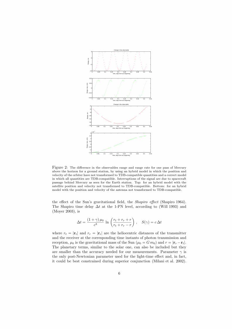
The total amount of the Shapiro effect in range is shown in Figure 3.

0 100 200 300 400 500 600 700 8000

0.5

1

1.5

2

2.5x 10

6 Change in the observable

time, days from arc beginning

Ran

ge, c

m

Figure 3: Total amount of the Shapiro effect in range over 2-year simulation. The sharppeaks correspond to superior conjunctions, when Mercury is “behind the Sun” as seen fromEarth, with values as large as 24 km for radio waves passing at 3 solar radii from the centerof the Sun. Interruptions of the signal are due to spacecraft visibility from the Earth station(in this simulation we assume just one station).

The question arises whether the very high signal to noise in the range requiresother terms in the solar gravity influence, due to either (i) motion of the source,or (ii) higher-order corrections when the radio waves are passing near the Sun,at just a few solar radii (and thus the denominator in the log-function of theShapiro formula is small). The corrections (i) are of the post-Newtonian order1.5 (containing a factor 1/c3), but it has been shown in (Milani et al. 2010)that they are too small to affect our accuracy. The corrections (ii) are of order2, (containing a factor 1/c4), but they can be actually larger for an experimentinvolving Mercury. The relevant correction is most easily obtained by adding1/c4 terms in the Shapiro formula, due to the bending of the light path:

S(γ) =(1 + γ)µ0

c2ln

(

rt + rr + r + (1+γ) µ0

c2

rt + rr − r + (1+γ) µ0

c2

)

.

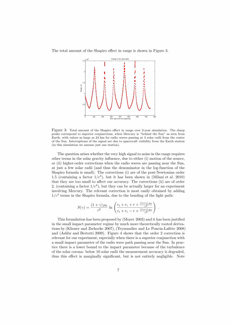
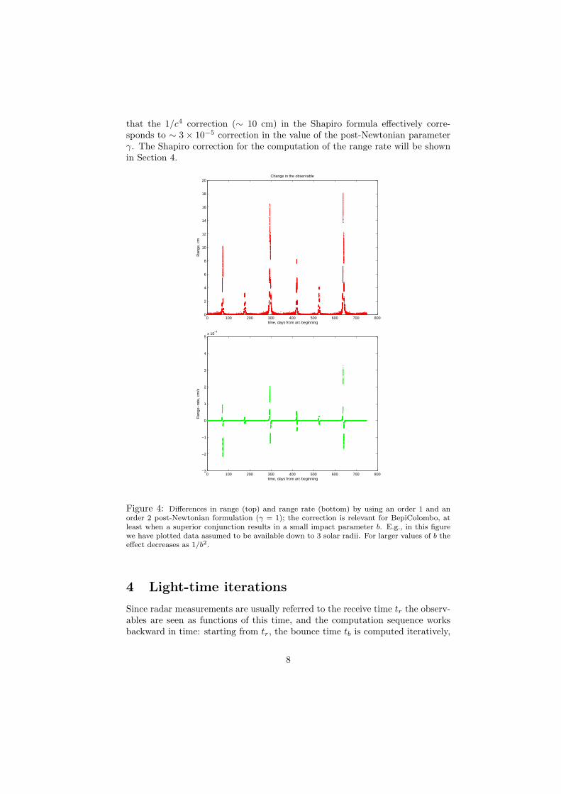
This formulation has been proposed by (Moyer 2003) and it has been justifiedin the small impact parameter regime by much more theoretically rooted deriva-tions by (Klioner and Zschocke 2007), (Teyssandier and Le Poncin-Lafitte 2008)and (Ashby and Bertotti 2009). Figure 4 shows that the order 2 correction isrelevant for our experiment, especially when there is a superior conjunction witha small impact parameter of the radio wave path passing near the Sun. In prac-tice there is a lower bound to the impact parameter because of the turbulenceof the solar corona: below 10 solar radii the measurement accuracy is degraded,thus this effect is marginally significant, but is not entirely negligible. Note

7

that the 1/c4 correction (∼ 10 cm) in the Shapiro formula effectively corre-sponds to ∼ 3 × 10−5 correction in the value of the post-Newtonian parameterγ. The Shapiro correction for the computation of the range rate will be shownin Section 4.

0 100 200 300 400 500 600 700 8000

2

4

6

8

10

12

14

16

18

20Change in the observable

time, days from arc beginning

Ran

ge, c

m

0 100 200 300 400 500 600 700 800−3

−2

−1

0

1

2

3

4

5x 10

−4

time, days from arc beginning

Ran

ge−

rate

, cm

/s

Figure 4: Differences in range (top) and range rate (bottom) by using an order 1 and anorder 2 post-Newtonian formulation (γ = 1); the correction is relevant for BepiColombo, atleast when a superior conjunction results in a small impact parameter b. E.g., in this figurewe have plotted data assumed to be available down to 3 solar radii. For larger values of b theeffect decreases as 1/b2.

4 Light-time iterations

Since radar measurements are usually referred to the receive time tr the observ-ables are seen as functions of this time, and the computation sequence worksbackward in time: starting from tr, the bounce time tb is computed iteratively,

8

and, using this information the transmit time tt is computed.The vectors xTB

M and xTBEM are obtained integrating the post-Newtonian equa-

tions of motion. The vectors xTMsat are obtained by integrating the orbit in the

mercurycentric TDM-compatible frame. The vector xTTant is obtained from a

standard IERS model of Earth rotation, given accurate station coordinates,and xTT

E from lunar ephemerides (Milani and Gronchi 2010). In the followingsubsections we shall describe the procedure to compute the range (Section 4.1)and the range rate (Section 4.2).

4.1 Range

Once the five vectors are available at the appropriate times and in a consistentSSB system, there are two different light-times, the up-leg ∆tup = tb − tt forthe signal from the antenna to the orbiter, and the down-leg ∆tdown = tr − tbfor the return signal. They are defined implicitly by the distances down-leg andup-leg

rdo(tr) = xsat(tb(tr)) + xM(tb(tr)) − xEM(tr) − xE(tr) − xant(tr) ,

rdo(tr) = |rdo(tr)| , c(tr − tb) = rdo(tr) + Sdo(γ) , (3)

rup(tr) = xsat(tb(tr)) + xM(tb(tr)) − xEM(tt(tr)) − xE(tt(tr)) − xant(tt(tr)) ,

rup(tr) = |rup(tr)| , c(tb − tt) = rup(tr) + Sup(γ) , (4)

respectively, with somewhat different Shapiro effects:

Sdo(γ) =(1 + γ)µ0

c2ln

(

rt(tb) + rr(tr) + |rr(tr) − rt(tb)| +(1+γ) µ0

c2

rt(tb) + rr(tr) − |rr(tr) − rt(tb)| +(1+γ) µ0

c2

)

,

Sup(γ) =(1 + γ)µ0

c2ln

(

rt(tt) + rr(tb) + |rr(tb) − rt(tt)| +(1+γ) µ0

c2

rt(tt) + rr(tb) − |rr(tb) − rt(tt)| +(1+γ) µ0

c2

)

.

Note that, for the down-leg, the vector rt refers to the heliocentric position ofthe spacecraft and it is computed at the bounce time, while, for the up-leg, thesame vector refers to the heliocentric position of the antenna and it is computedat the transmit time. This difference occurs also for the vector rr: in the down-leg it refers to the position of the antenna at the receive time, while in the up-legto the position of the spacecraft at the bounce time.

Then tr − tb and tb− tt are the two portions of the light-time, in the time at-tached to the SSB, that is TDB; this provides the computation of tt. Then thesetimes are to be converted back in the time system applicable at the receivingstation, where the time measurement is performed, which is TT (or some otherform of local time, such as the standard UTC). The time tr is already availablein the local time scale, from the original measurement, while tt needs to beconverted back from TDB to TT. The difference between these two TT timesis ∆ttot, from which we can conventionally define r(tr) = c∆ttot/2. Note that

9

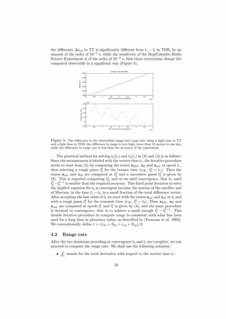
the difference ∆ttot in TT is significantly different from tr − tt in TDB, by anamount of the order of 10−7 s, while the sensitivity of the BepiColombo RadioScience Experiment is of the order of 10−9 s, thus these conversions change thecomputed observable in a significant way (Figure 5).

0 0.5 1 1.5 2 2.5 3 3.5 4

x 104

−1380

−1370

−1360

−1350

−1340

−1330Change in the observable

time, seconds from arc beginning

Ran

ge, c

m

0 0.5 1 1.5 2 2.5 3 3.5 4

x 104

1.08

1.1

1.12

1.14

1.16

1.18x 10

−7

time, seconds from arc beginning

Ran

ge−

rate

, cm

/s

Figure 5: The difference in the observables range and range rate using a light-time in TTand a light time in TDB: the difference in range is very high, more than 13 meters in one day,while the difference in range rate is less than the accuracy of the experiment.

The practical method for solving tb(tr) and tt(tr) in (3) and (4) is as follows.Since the measurement is labeled with the receive time tr, the iterative procedureneeds to start from (3) by computing the states xEM, xE and xant at epoch tr,then selecting a rough guess t0b for the bounce time (e.g., t0b = tr). Then thestates xsat and xM are computed at t0b and a successive guess t1b is given by(3). This is repeated computing t2b , and so on until convergence, that is, untiltkb −tk−1

b is smaller than the required accuracy. This fixed point iteration to solvethe implicit equation for tb is convergent because the motion of the satellite andof Mercury, in the time tr − tb, is a small fraction of the total difference vector.After accepting the last value of tb we start with the states xsat and xM at tb andwith a rough guess t0t for the transmit time (e.g., t0t = tb). Then xEM, xE andxant are computed at epoch t0t and t1t is given by (4), and the same procedureis iterated to convergence, that is to achieve a small enough tkt − tk−1

t . Thisdouble iterative procedure to compute range is consistent with what has beenused for a long time in planetary radar, as described in (Yeomans et al. 1992).We conventionally define r = (rdo + Sdo + rup + Sup)/2.

4.2 Range rate

After the two iterations providing at convergence tb and tt are complete, we canproceed to compute the range rate. We shall use the following notation:

• ddtr

stands for the total derivative with respect to the receive time tr;

10

• ∂∂tb

stands for the partial derivative with respect to the receive time tb;

• ∂∂tt

stands for the partial derivative with respect to the receive time tt.

We rewrite the expression for the Euclidean range (down-leg and up-leg) as ascalar product:

r2do(tr) = [xMs(tb) − xEa(tr)] · [xMs(tb) − xEa(tr)] ,

r2up(tr) = [xMs(tb) − xEa(tt)] · [xMs(tb) − xEa(tt)] ,

where xMs = xM + xsat and xEa = xEM + xE + xant. The light-time equationcontains also the Shapiro terms, thus the range rate observable contains alsoadditive terms dSdo/dtr and dSup/dtr, with significant effects (a few cm/s duringsuperior conjunctions). Since the equations giving tb and tt are still (3) and (4),in computing the time derivatives, we need to take into account that tb = tb(tr)and tt = tt(tr), with non-unit derivatives. By computing the derivative withrespect to the receive time tr we obtain

d

dtr[rdo(tr) + Sdo(tr)] = rdo ·

[

∂xMs(tb)

∂tb

dtbdtr

−dxEa(tr)

dtr

]

+dSdo

dtr(5)

where

rdo =xMs(tb) − xEa(tr)

rdo(tr),

dtbdtr

= 1 −drdo(tr)/dtr + dSdo/dtr

c

and

d

dtr[rup(tr) + Sup(tr)] = rup ·

[

∂xMs(tb)

∂tb

dtbdtr

−∂xEa(tt)

∂tt

dttdtr

]

+dSup

dtr(6)

where

rup =xMs(tb) − xEa(tt)

rup(tr),

dttdtr

= 1 −drdo(tr)/dtr + dSdo/dtr

c−

drup(tr)/dtr + dSup/dtrc

.

The derivatives of the Shapiro effect are

dSdo

dtr=

2 (1 + γ)µ0

c2

[

(

rt(tb) + rr(tr) +(1 + γ)µ0

c2

)2

− |rr(tr) − rt(tb)|2

]

−1

(7)

[

− |rr(tr) − rt(tb)|

(

∂rt

∂tb

dtbdtr

+drr

dtr

)

+

rr(tr) − rt(tb)

|rr(tr) − rt(tb)|·

(

drr

dtr−

∂rt

∂tb

dtbdtr

) (

rt(tb) + rr(tr) +(1 + γ)µ0

c2

)

]

,

11

dSup

dtr=

2 (1 + γ)µ0

c2

[

(

rt(tt) + rr(tb) +(1 + γ)µ0

c2

)2

− |rr(tb) − rt(tt)|2

]

−1

(8)

[

− |rr(tb) − rt(tt)|

(

∂rt

∂tt

dttdtr

+∂rr

∂tb

dtbdtr

)

+

rr(tb) − rt(tt)

|rr(tr) − rt(tb)|·

(

∂rr

∂tb

dtbdtr

−∂rt

∂tt

dttdtr

) (

rt(tt) + rr(tb) +(1 + γ)µ0

c2

)

]

.

Note that, because of different definitions of rt and rr in the down-leg andup-leg (Section 4.1), the term ∂rt/∂tb in the second row of (7) is exactly thesame thing as ∂rr/∂tb in the second row of (8). However, the contribution ofthe time derivatives of the Shapiro effect to the d tb/d tr and d tt/d tr correctivefactors is small, of the order of 10−10, which is marginally significant for theBepiColombo Radio Science Experiment. We conventionally define the rangerate dr/dtr = c(1−dtt/dtr)/2 = (drdo/dtr +dSdo/dtr +drup/dtr +dSup/dtr)/2.These equations are compatible with the equations in (Yeomans et al. 1992),taking into account that they use a single iteration. Equations (7) and (8)are almost never found in the literature and has not been much used in theprocessing of the past radio science experiments (Bertotti et al. 2003) becausethe observable range rate is typically computed as difference of ranges dividedby time; however, for reasons explained in Section 5, these formulas are nownecessary.

Since the time derivatives of the Shapiro effects contain dtb/dtr and dtt/dtr,the equations (5) and (6) are implicit, thus we can again use a fixed point itera-tion. It is also possible to use a very good approximation which solves explicitlyfor drdo/dtr and then for drup/dtr, neglecting the very small contribution ofShapiro terms:

drdo

dtr= rdo·

[

∂xMs(tb)

∂tb

(

1 −dSdo/dtr

c

)

−dxEa(tr)

dtr

] [

1 +1

c

(

∂xMs(tb)

∂tb· rdo

)]

−1

,

where the right hand side is weakly dependent upon drdo/dtr only throughdSdo/dtr, thus a moderately accurate approximation could be used in the com-putation of dSdo/dtr, followed by a single iteration. For the other leg

drup

dtr= rup ·

[

∂xMs(tb)

∂tb

(

1 −drdo(tr)/dtr + dSdo/dtr

c

)

−

∂xEa(tt)

∂tt

(

1 −drdo(tr)/dtr + dSdo/dtr + dSup/dtr

c

)

]

[

1 −1

c

(

∂xEa(tt)

∂tt· rup

)]

−1

All the above computations are in SSB with TDB; however, the frequency mea-surements, at both tt and tr, are done on Earth, that is with a time which is

12

TT. This introduces a change in the measured frequencies at both ends, andbecause this change is not the same (the Earth having moved by about 3×10−4

of its orbit) there is a correction needed to be performed. The quantity weare measuring is essentially the derivative of tt with respect to tr, but in twodifferent time systems (for readability, we use T for TT, t for TDB):

dTt

dTr=

dTt

dtt

dttdtr

dtrdTr

,

where the derivatives of the time coordinate changes are the same as the righthand side of the differential equation giving T as a function of t in the firstfactor and the inverse of the same for the last factor. However, the accuracyrequired is such that the main term with the gravitational mass of the Sun µ0

and the position of the Sun x0 is enough:

dTt

dTr=

[

1 −µ0

|xE(tt) − x0(tt)| c2−

1

2 c2

∣

∣

∣

∣

dxE(tt)

dtt

∣

∣

∣

∣

2]

dttdtr

[

1 −µ0

|xE(tr) − x0(tr)| c2−

1

2 c2

∣

∣

∣

∣

dxE(tr)

dtr

∣

∣

∣

∣

2]

−1

. (9)

Note that we do not need the LC constant term discussed in Section 2 because itcancels in the first and last term in the right hand side of (9). The correction ofthe above formula is required for consistency, but the correction has an order ofmagnitude of 10−7 cm/s and is negligible for the sensitivity of the BepiColomboRadio Science Experiment (Figure 5).

5 Numerical problems and solutions

The computation of the observables, as presented in the previous section, is al-ready complex, but still the list of subtle technicalities is not complete. A prob-lem well known in radio science is that, for top accuracy, the range rate measure-ment cannot be the value dr(tr)/dtr = (drdo(tr)/dtr +dSdo/dtr +drup(tr)/dtr +dSup/dtr)/2. In fact, the measurement is not instantaneous: an accurate mea-sure of a Doppler effect requires to fit the difference of phase between carrierwaves, the one generated at the station and the one returned from space, accu-mulated over some integration time ∆, typically between 10 and 1000 s. Thusthe observable is really a difference of ranges

r(tb + ∆/2) − r(tb − ∆/2)

∆(10)

or, equivalently, an averaged value of range rate over the integration interval

1

∆

∫ tb+∆/2

tb−∆/2

dr(s)

dtrds . (11)

13

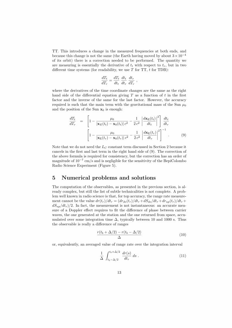
In order to understand the computational difficulty we need to take also intoaccount the orders of magnitude. As said in the introduction, for state of theart of tracking systems, such as those using a multi-frequency link in the X andKa bands, the accuracy of the range measurements can be ≃ 10 cm and theone of range-rate 3 × 10−4 cm/s (over an integration time of 1 000 s). Let ustake an integration time ∆ = 30 s, which is adequate for measuring the gravityfield of Mercury: in fact, if the orbital period of the spacecraft around Mercuryis ≃ 8 000 s, the harmonics of order m = 26 have periods as short as ≃ 150s. The accuracy over 30 s of the range rate measurement can be, by Gaussianstatistics, ≃ 3 × 10−4

√

1 000/30 ≃ 17 × 10−4 cm/s, and the required accuracyin the computation of the difference r(tb +∆/2)−r(tb−∆/2) is ≃ 0.05 cm. Thedistances can be as large as ≃ 2×1013 cm, thus the relative accuracy in the dif-ference needs to be 2.5×10−15. This implies that rounding off is a problem withcurrent computers, with relative rounding off error of ε = 2−52 = 2.2 × 10−16

(Figure 6); extended precision is supported in software, but it has many limi-tations. The practical consequences are that the computer program processingthe tracking observables, at this level of precision and over interplanetary dis-tances, needs to be a mixture of ordinary and extended precision variables. Anyimperfection may result in “banding”, that is residuals showing a discrete setof values, implying that some information corresponding to the real accuracy ofthe measurements has been lost in the digital processing.

0 0.5 1 1.5 2 2.5 3 3.5 4

x 104

−0.2

−0.1

0

0.1

0.2Change in the observable

time, seconds from arc beginning

Ran

ge, c

m

0 0.5 1 1.5 2 2.5 3 3.5 4

x 104

−6

−4

−2

0

2

4x 10

−4

time, seconds from arc beginning

Ran

ge−

rate

, cm

/s

Figure 6: Range and range rate differences due to a change by 10−11 of the C22 harmoniccoefficient: the range rate computed as range difference divided by the integration time of 30s is obscured by the rounding off.

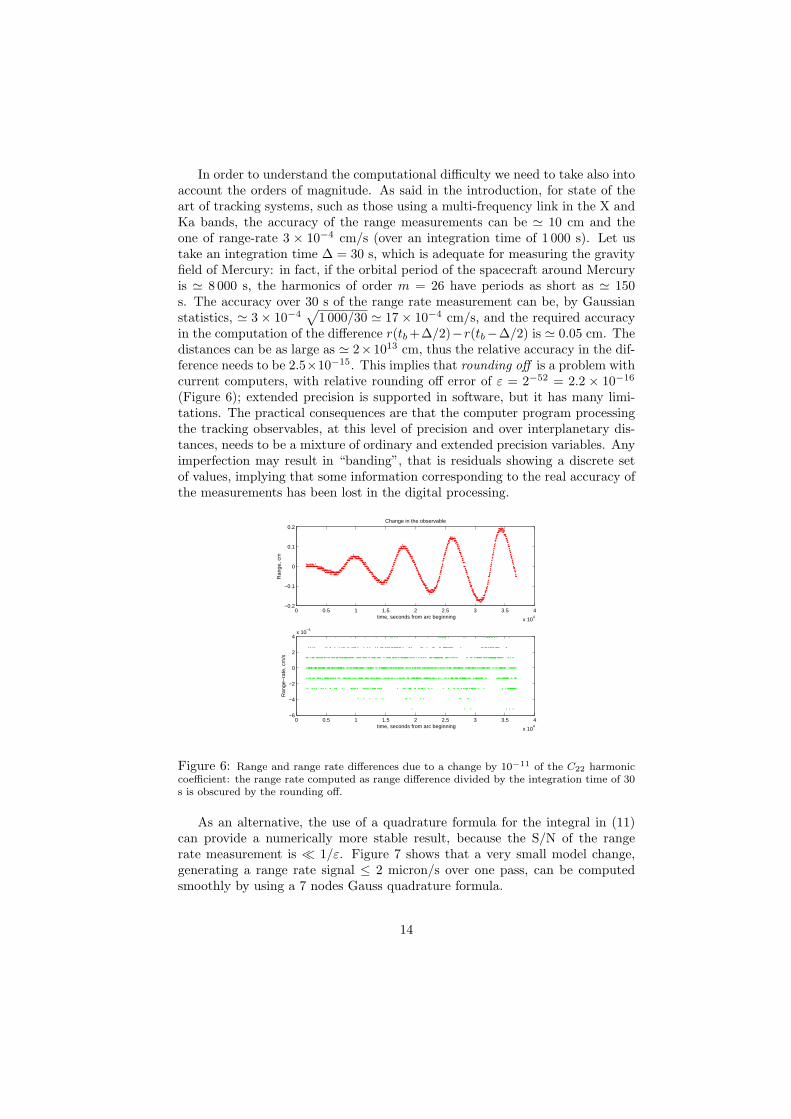
As an alternative, the use of a quadrature formula for the integral in (11)can provide a numerically more stable result, because the S/N of the rangerate measurement is ≪ 1/ε. Figure 7 shows that a very small model change,generating a range rate signal ≤ 2 micron/s over one pass, can be computedsmoothly by using a 7 nodes Gauss quadrature formula.

14

0 0.5 1 1.5 2 2.5 3 3.5 4

x 104

−0.2

−0.1

0

0.1

0.2Change in the observable

time, seconds from arc beginning

Ran

ge, c

m

0 0.5 1 1.5 2 2.5 3 3.5 4

x 104

−1.5

−1

−0.5

0

0.5

1

1.5

2x 10

−4

time, seconds from arc beginning

Ran

ge−

rate

, cm

/s

Figure 7: Range and range rate differences due to a change by 10−11 of the C22 harmoniccoefficient: the range rate computed as an integral is smooth; the difference is marginallysignificant with respect to the measurement accuracy.

6 Conclusions

By combining the results of (Milani et al. 2010) and of this paper, we have com-pleted the task of showing that it is possible to build a consistent relativisticmodel of the dynamics and of the observations for a Mercury orbiter trackedfrom the Earth, at a level of accuracy and self-consistency compatible with thevery demanding requirements of the BepiColombo Radio Science Experiment.In particular, in this paper we have defined the algorithms for the computationof the observables range and range rate, including the reference system effectsand the Shapiro effect. We have shown which computations can be performedexplicitly and which ones need to be obtained from an iterative procedure. Wehave also shown how to push these computations, when implemented in a real-istic computer with rounding-off, to the needed accuracy level, even without thecumbersome usage of quadruple precision. The list of “relativistic corrections”,assuming that we can distinguish their effects separately, is long, and we haveshown that many subtle effects are relevant to the required accuracy. However,in the end what is required is just to be fully consistent with a post-Newtonianformulation to some order, to be adjusted when necessary. Interestingly, thehigh accuracy of BepiColombo radio system may require implementation of thesecond post-Newtonian effects in range.

Acknowledgements The authors thank the anonymous reviewer for his construc-

tive comments useful to improve the presentation of the work. The results of the

research presented in this paper, as well as in the previous one (Milani et al. 2010),

have been performed within the scope of the contract ASI/2007/I/082/06/0 with the

Italian Space Agency. BepiColombo is a scientific space mission of the Science Direc-

torate of the European Space Agency. The work of DV was partially supported by the

15

Czech Grant Agency (grant 202/09/0772) and the Research Program MSM0021620860

of the Czech Ministry of Education.

References

[Ashby and Bertotti 2009] Ashby, N., Bertotti, B.: Accurate light-time correc-tion due to a gravitating mass, ArXiv e-prints, 0912.2705 (2009)

[Bertotti et al. 2003] Bertotti, B., Iess, L., Tortora, P.: A test of general rela-tivity using radio links with the Cassini spacecraft. Nature, 425, 374-376(2003)

[Damour et al. 1994] Damour, T., Soffel, M., Hu, C.: General-relativistic celes-tial mechanics. IV. Theory of satellite motion. Phys. Rev. D, 49, 618-635(1994)

[Iess and Boscagli 2001] Iess, L., Boscagli, G.: Advanced radio science instru-mentation for the mission BepiColombo to Mercury. Plan. Sp. Sci., 49,1597-1608 (2001)

[Klioner and Zschocke 2007] Klioner, S.A., Zschocke, S.: GAIA-CA-TN-LO-SK-002-1 report (2007)

[Klioner 2008] Klioner, S.A.: Relativistic scaling of astronomical quantities andthe system of astronomical units. Astron. Astrophys., 478, 951–958 (2008)

[Klioner et al. 2010] Klioner, S.A., Capitaine, N., Folkner, W., Guinot, B.,Huang, T. Y., Kopeikin, S., Petit, G., Pitjeva, E., Seidelmann, P. K.,Soffel, M.: Units of Relativistic Time Scales and Associated Quantities.In: Klioner, S., Seidelmann, P.K., Soffel, M. (eds.) Relativity in Funda-mental Astronomy: Dynamics, Reference Frames, and Data Analysis, IAUSymposium, 261, 79-84 (2010)

[Milani et al. 2002] Milani, A., Vokrouhlicky, D., Villani, D., Bonanno, C.,Rossi, A.: Testing general relativity with the BepiColombo radio scienceexperiment. Phys. Rev. D, 66, 082001 (2002)

[Milani and Gronchi 2010] Milani A., Gronchi G.F.: Theory of orbit determi-nation. Cambridge University Press (2010)

[Milani et al. 2010] Milani, A., Tommei, G., Vokrouhlicky, D., Latorre, E., Ci-calo, S.: Relativistic models for the BepiColombo radioscience experiment.In: Klioner, S., Seidelmann, P.K., Soffel, M. (eds.) Relativity in Funda-mental Astronomy: Dynamics, Reference Frames, and Data Analysis, IAUSymposium, 261, 356-365 (2010)

[Moyer 2003] Moyer, T.D.: Formulation for Observed and Computed Values ofDeep Space Network Data Types for Navigation. Wiley-Interscience (2003)

16

[Shapiro 1964] Shapiro, I.I.: Fourth test of general relativity. Phys. Rev. Lett.,13, 789-791 (1964)

[Soffel et al. 2003] Soffel, M., Klioner, S.A., Petit, G., Kopeikin, S.M., Bre-tagnon, P., Brumberg, V.A., Capitaine, N., Damour, T., Fukushima, T.,Guinot, B., Huang, T.-Y., Lindegren, L., Ma, C., Nordtvedt, K., Ries,J.C., Seidelmann, P.K., Vokrouhlicky, D., Will, C.M., Xu, C.: The IAU2000 resolutions for astrometry, celestial mechanics, and metrology in therelativistic framework: explanatory supplement. Astron. J., 126, 2687-2706(2003)

[Teyssandier and Le Poncin-Lafitte 2008] Teyssandier, P., Le Poncin-Lafitte,C.: General post-Minkowskian expansion of time transfer functions. Class.Quantum Grav., 25, 145020 (2008)

[Will 1993] Will, C.M.: Theory and experiment in gravitational physics. Cam-bridge University Press (1993)

[Yeomans et al. 1992] Yeomans, D. K., Chodas, P. W., Keesey, M. S., Ostro, S.J., Chandler, J. F., Shapiro, I. I.: Asteroid and comet orbits using radardata. Astron. J., 103, 303-317 (1992)

17