Lifetime-Based Memory Management for Distributed DataProcessing Systems

Lu Lu †, Xuanhua Shi †∗, Yongluan Zhou ‡∗, Xiong Zhang †, Hai Jin †, Cheng Pei †, Ligang He §, Yuanzhen Geng ††Services Computing Technology and System Lab / Big Data Technology and System Lab

Huazhong University of Science and Technology, China‡University of Southern Denmark, Denmark §University of Warwick, UK

†{llu,xhshi,hjin,wxzhang,peicheng,yzgeng}@hust.edu.cn, ‡zhou@imada.sdu.dk, § liganghe@dcs.warwick.ac.uk

ABSTRACTIn-memory caching of intermediate data and eager combin-ing of data in shuffle buffers have been shown to be very ef-fective in minimizing the re-computation and I/O cost in dis-tributed data processing systems like Spark and Flink. How-ever, it has also been widely reported that these techniqueswould create a large amount of long-living data objects inthe heap, which may quickly saturate the garbage collec-tor, especially when handling a large dataset, and hencewould limit the scalability of the system. To eliminate thisproblem, we propose a lifetime-based memory managementframework, which, by automatically analyzing the user-defined functions and data types, obtains the expected life-time of the data objects, and then allocates and releasesmemory space accordingly to minimize the garbage collec-tion overhead. In particular, we present Deca, a concrete im-plementation of our proposal on top of Spark, which trans-parently decomposes and groups objects with similar life-times into byte arrays and releases their space altogetherwhen their lifetimes come to an end. An extensive experi-mental study using both synthetic and real datasets showsthat, in comparing to Spark, Deca is able to 1) reduce thegarbage collection time by up to 99.9%, 2) to achieve up to22.7x speed up in terms of execution time in cases withoutdata spilling and 41.6x speedup in cases with data spilling,and 3) to consume up to 46.6% less memory.

1. INTRODUCTIONDistributed data processing systems, such as Spark [34],

process huge volumes of data in a scale-out fashion. Unliketraditional database systems using declarative query lan-guages and relational (or multidimensional) data models,these systems allow users to implement application logicsthrough User Defined Functions (UDFs) and User DefinedTypes (UDTs) using high-level imperative languages (suchas Java, Scala and C#), which can then be automaticallyparallelized onto a large-scale cluster.

∗Corresponding author

This work is licensed under the Creative Commons Attribution-NonCommercial-NoDerivatives 4.0 International License. To view a copyof this license, visit http://creativecommons.org/licenses/by-nc-nd/4.0/. Forany use beyond those covered by this license, obtain permission by emailinginfo@vldb.org.Proceedings of the VLDB Endowment, Vol. 9, No. 12Copyright 2016 VLDB Endowment 2150-8097/16/08.

Existing researches in these systems mostly focus on scal-ability and fault-tolerance issues in a distributed environ-ment [10, 18, 35]. However some recent studies [11, 24]suggest that the execution efficiency of individual tasks inthese systems is low. A major reason is that both the exe-cution frameworks and user programs of these systems areimplemented using high-level imperative languages runningin managed runtime platforms (such as JVM and .NETCLR). These managed runtime platforms commonly havebuilt-in automatic memory management, which brings sig-nificant memory and CPU overheads in exchange for theease of programming [5, 15, 19].

Furthermore, to improve the performance of multi-stageand iterative computations, recently developed systems sup-port caching of intermediate data in the main memory [28,31, 34] and exploit eager combining and aggregating of datain the shuffling phases [21, 30]. These techniques wouldgenerate massive long-living data objects in the heap, whichusually stay in the memory for a significant portion of thejob execution time. However, the unnecessary continuoustracing and marking of such large amount of long-living ob-jects by the modern tracing-based garbage collectors (GC)would consume significant CPU cycles.

In this paper, we argue that distributed data processingsystems like Spark, should employ a lifetime-based memorymanager, which allocates and releases memory according tothe lifetimes of the data objects rather than relying on aconventional tracing-based GC. To verify this concept, wepresent Deca, an automatic Spark optimizer, which adoptsa lifetime-based memory management scheme for efficientlyreclaiming memory space. Deca automatically analyzes thelifetimes of objects in different data containers in Spark, suchas UDF variables, cached data blocks and shuffle buffers, andthen transparently decomposes and stores a massive numberof objects with similar lifetimes into a few number of bytearrays. In this way, the massive objects essentially bypassthe continuous tracing of the GC and their space can bereleased by the destruction of the byte arrays.

Last but not the least, Deca automatically transforms theuser programs so that the new memory layout is transpar-ent to the users. By using the aforementioned techniques,Deca significantly optimizes the efficiency of Spark’s mem-ory management and at the same time keeps the generalityand expressibility provided in Spark’s programming model.In summary, the main contributions of this paper include:

• We propose a lifetime-based memory managementscheme for distributed data processing systems and im-plement a prototype on top of Spark, which is able to

936

minimize the GC overhead and eliminate the memorybloat problems in Spark.

• We design a method that changes the in-memory rep-resentation of the object graph of each data item bydiscarding all the reference values. The raw data ofthe fields of primitive types in the object graph will becompactly stored as a byte sequence.

• We propose techniques to group byte sequences of dataitems with the same lifetime into a few byte arrays,thereby simplifying space reclamation. Deca automat-ically validates the memory safety of data accessingbased on analysis of memory usage of UDT objects.

• We conduct extensive evaluation on various Spark pro-grams using both synthetic and real datasets. The ex-perimental results demonstrate the superiority of ourapproach by comparing with existing methods.

2. OVERVIEW OF DECA

2.1 Java GCIn typical JVM implementations, a garbage collector at-

tempts to reclaim memory occupied by objects that willno longer be used. A tracing GC traces objects which arereachable by a sequence of references from some root ob-jects. The unreachable ones, which are called garbages, canbe reclaimed. Oracle’s Hotspot JVM implements three GCalgorithms. The default Parallel Scavenge (PS) algorithmsuspends the application and spawns several parallel GCthreads to achieve high throughput. The other two algo-rithms, namely Concurrent Mark-Sweep (CMS) and Garbage-First (G1), attempt to reduce GC latency by spawning con-current GC threads that run simultaneously with the appli-cation threads.

All the above collectors segregate objects into multiplegenerations according to their “ages”. Based on the assump-tion that most objects would soon become garbages, a minorGC, which only attempts to reclaim garbages in the younggeneration, can be run to reclaim enough memory space.However, if there are too many old objects, then a full (ormajor) GC would be run to reclaim space occupied by theold objects. Usually, a full GC is much more expensive thana minor GC.

2.2 Motivating ExampleA major concept of Spark is Resilient Distributed Dataset

(RDD), which is a fault-tolerant dataset that can be pro-cessed in parallel by a set of UDF operations.

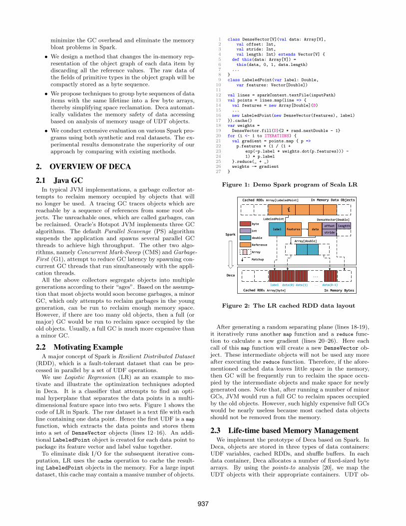
We use Logistic Regression (LR) as an example to mo-tivate and illustrate the optimization techniques adoptedin Deca. It is a classifier that attempts to find an opti-mal hyperplane that separates the data points in a multi-dimensional feature space into two sets. Figure 1 shows thecode of LR in Spark. The raw dataset is a text file with eachline containing one data point. Hence the first UDF is a map

function, which extracts the data points and stores theminto a set of DenseVector objects (lines 12–16). An addi-tional LabeledPoint object is created for each data point topackage its feature vector and label value together.

To eliminate disk I/O for the subsequent iterative com-putation, LR uses the cache operation to cache the result-ing LabeledPoint objects in the memory. For a large inputdataset, this cache may contain a massive number of objects.

1 class DenseVector[V](val data: Array[V],2 val offset: Int,3 val stride: Int,4 val length: Int) extends Vector[V] {5 def this(data: Array[V]) =6 this(data, 0, 1, data.length)7 ...8 }9 class LabeledPoint(var label: Double,

10 var features: Vector[Double])1112 val lines = sparkContext.textFile(inputPath)13 val points = lines.map(line => {14 val features = new Array[Double](D)15 ...16 new LabeledPoint(new DenseVector(features), label)17 }).cache()18 var weights =19 DenseVector.fill(D){2 * rand.nextDouble - 1}20 for (i <- 1 to ITERATIONS) {21 val gradient = points.map { p =>22 p.features * (1 / (1 +23 exp(-p.label * weights.dot(p.features))) -24 1) * p.label25 }.reduce(_ + _)26 weights -= gradient27 }

Figure 1: Demo Spark program of Scala LR

...

i

featureslabel

double

Reference

Cached RDD：Array[LabeledPoint]

Array

byte

Cached RDD：Array[byte]

label data(0) data(1) data(D-1)...

int

offsetdata

stride

lenghth

LabeledPoint DenseVector[Double]

Array[double]

Spark

Deca

In Memory Data Objects

In Memory Bytes

Matchup

Figure 2: The LR cached RDD data layout

After generating a random separating plane (lines 18-19),it iteratively runs another map function and a reduce func-tion to calculate a new gradient (lines 20–26). Here eachcall of this map function will create a new DenseVector ob-ject. These intermediate objects will not be used any moreafter executing the reduce function. Therefore, if the afore-mentioned cached data leaves little space in the memory,then GC will be frequently run to reclaim the space occu-pied by the intermediate objects and make space for newlygenerated ones. Note that, after running a number of minorGCs, JVM would run a full GC to reclaim spaces occupiedby the old objects. However, such highly expensive full GCswould be nearly useless because most cached data objectsshould not be removed from the memory.

2.3 Life-time based Memory ManagementWe implement the prototype of Deca based on Spark. In

Deca, objects are stored in three types of data containers:UDF variables, cached RDDs, and shuffle buffers. In eachdata container, Deca allocates a number of fixed-sized bytearrays. By using the points-to analysis [20], we map theUDT objects with their appropriate containers. UDT ob-

937

jects are then stored in the byte arrays after eliminatingthe unnecessary object headers and object references. Thiscompact layout would not only minimize the memory con-sumption of data objects but also dramatically reduce theoverhead of GC, because GC only needs to trace a few bytearrays instead of a huge number of UDT objects. One cansee that the size of each byte array should not be too smallor too large, otherwise it would incur high GC overheads orlarge unused memory spaces.

As an example, the LabeledPoint objects in the LR pro-gram can be transformed into byte arrays as shown in Fig-ure 2. Here, all the reference variables (in orange color, suchas features and data), as well as the headers of all the ob-jects are eliminated. All the cached LabeledPoint objectsare stored into byte arrays.

The challenge of employing such a compact layout is thatthe space allocated to each object is fixed. Therefore, wehave to ensure that the size of an object would not exceedits allocated space during execution so that it will not dam-age the data layout. This is easy for some types of fields,such as primitive types, but less obvious for others. Codeanalysis is necessary to identify the change patterns of theobjects’ sizes. Such an analysis may have a global scope.For example, a global code analysis may identify that thefeatures arrays of all the LabeledPoint objects (created inline 14 in Figure 1) actually have the same fixed size D, whichis a global constant. Furthermore, the features field of aLabeledPoint object is only assigned in the LabeledPoint

constructor. Therefore, all the LabeledPoint objects actu-ally have the same fixed size. Another interesting pattern isthat in Spark applications, objects in cached RDDs or shufflebuffers are often generated sequentially and their sizes willnot be changed once they are completely generated. Identi-fying such useful patterns by a sophisticated code analysis isnecessary to ensure the safety of decomposing UDT objectsand storing them compactly into byte arrays.

As mentioned earlier, during the execution of programsin a system like Spark, the lifetimes of data containers cre-ated by the framework can be pre-determined explicitly. Forexample, the lifetimes of objects in a cached RDD is deter-mined by the invocations of cache() and unpersist() in theprogram. Recall that the UDT objects stored in the compactbyte arrays would bypass the GC. We put the UDT objectswith the same lifetime into the same container. For exam-ple, the cached LabeledPoint objects in LR have the samelifetime, so they are stored in the same container. When acontainer’s lifetime comes to an end, we simply release allthe references of the byte arrays in the container, then theGC can reclaim the whole space occupied by the massiveamount of objects.

Lastly, Deca modifies the application code by replacingthe codes of object creation, field access and UDT methodswith new codes that directly write and read the byte arrays.

3. UDT CLASSIFICATION ANALYSIS

3.1 Data-size and Size-type of ObjectsTo allocate enough memory space for objects, we have to

estimate the object sizes and their change patterns duringruntime. Due to the complexity of object models, to accu-rately estimate the size of a UDT, we have to dynamicallytraverse the runtime object reference graph of each targetobject and compute the total memory consumption. Such a

dynamic analysis is too costly at runtime, especially with alarge number of objects. Therefore we opt for static analysiswhich only uses static object reference graphs and would notincur any runtime overhead. We define the data-size of anobject to be the sum of the sizes of the primitive-type fieldsin its static object reference graph. An object’s data-size isonly an upper bound of the actual memory consumption ofits raw data, if one considers the cases with object sharing.

To see if UDT objects can be safely decomposed into bytesequences, we should examine how their data-sizes changeduring runtime. There are two types of UDTs that can meetthe safety requirement: 1) the data-sizes of all the instancesof the UDT are identical and do not change during runtime;or 2) the data-sizes of all the instances of the UDT do notchange during runtime. We call these two kinds of UDTs asStatic Fixed-Sized Type (SFST) and Runtime Fixed-Sized Type (RFST) respectively.

In addition, we call UDTs that have type-dependency cy-cles in their type definition graphs as Recursively-DefinedType. Even without object sharing, the instances of thesetypes can have reference cycles in their object graphs. There-fore, they cannot be safely decomposed. Furthermore, anyUDT that does not belong to any of the aforementionedtypes is called a Variable-Sized Type (VST). Once a VSTobject is constructed, its data-size may change due to fieldassignments and method invocations during runtime.

The objective of the UDT classification analysis is to gen-erate the Size-Type of each target UDT according to theabove definitions. As demonstrated in Figure 2, Deca de-composes a set of objects into primitive values and storesthem contiguously into compact byte sequences in a bytearray. A safe decomposition requires that the original UDTobjects are either of an SFST or an RFST. Otherwise theoperations that expand the byte sequences occupied by anobject may overwrite the data of the subsequent objects inthe same byte array. Furthermore, as we will discuss later,an SFST can be safely decomposed in more cases than anRFST. On the other hand, objects that do not belong toan SFST or an RFST will not be decomposed into byte se-quences in Deca. Apparently, to maximize the effect of ourapproach, we should avoid overestimating the variability ofthe data-size of the UDTs, which is the design goal of ourfollowing algorithms.

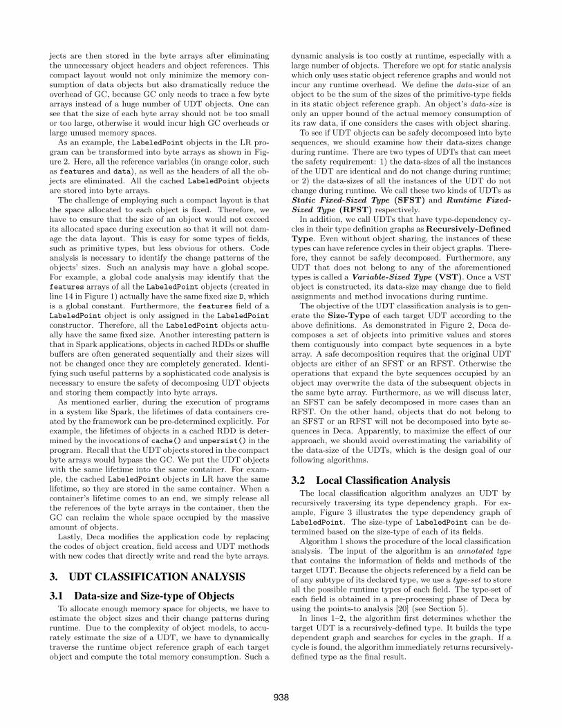
3.2 Local Classification AnalysisThe local classification algorithm analyzes an UDT by

recursively traversing its type dependency graph. For ex-ample, Figure 3 illustrates the type dependency graph ofLabeledPoint. The size-type of LabeledPoint can be de-termined based on the size-type of each of its fields.

Algorithm 1 shows the procedure of the local classificationanalysis. The input of the algorithm is an annotated typethat contains the information of fields and methods of thetarget UDT. Because the objects referenced by a field can beof any subtype of its declared type, we use a type-set to storeall the possible runtime types of each field. The type-set ofeach field is obtained in a pre-processing phase of Deca byusing the points-to analysis [20] (see Section 5).

In lines 1–2, the algorithm first determines whether thetarget UDT is a recursively-defined type. It builds the typedependent graph and searches for cycles in the graph. If acycle is found, the algorithm immediately returns recursively-defined type as the final result.

938

Algorithm 1: Local Classification Analysis

Input : The top-level annotated type T ;Output: The size-type of T ;

1 build the type dependency graph G for T ;2 if G contains the circle path then return RecurDef;3 else return AnalyzeType(T);

4 Function AnalyzeType(targ)5 if targ is a primitive type then return StaticFixed;6 else if targ is an array type then7 fe ← array element field of targ ;8 if AnalyzeField(fe) = StaticFixed then9 return RuntimeFixed;

10 else return Variable;

11 else12 result← StaticFixed;13 foreach field f of type targ do14 tmp← AnalyzeField(f);15 if tmp = Variable then return Variable;16 else if tmp = RuntimeFixed then17 result← RuntimeFixed;18 end

19 end20 return result;

21 end

22 end

23 Function AnalyzeField(farg)24 result← StaticFixed;25 foreach runtime type t in farg .getTypeSet do26 tmp← AnalyzeType(t);27 if tmp = Variable then return Variable;28 else if tmp = RuntimeFixed then29 if farg is not final then return Variable;30 else result← RuntimeFixed;

31 end32 end33 return result;34 end

Two indirect-recursive functions, AnalyzeType (lines 4–22) and AnalyzeField (lines 23–34), are used to further de-termine the size-type of the target UDT. The stop conditionof the recursion is when the current type is a primitive type(line 5). We treat each array type as having a length fieldand an element field. Since different instances of an arraytype can have different lengths, arrays with static fixed-sizedelements will be considered as an RFST (lines 8–9).

We define a total ordering of the variability of the size-types (except the recursively-defined type) as follows:SFST < RFST < V ST . Based on this order, the size-typeof each UDT is determined by its field that has the highestvariability (lines 12–20). Furthermore, each field’s final size-type is determined by the type with the highest variability inits type-set. But a non-final field of an RFST will be finallyclassified as VST, because the same field can possibly pointto objects with different data-sizes (lines 28-29). Considerthat whenever we find a VST field, the top-level UDT mustalso be classified as a VST. In this case, the function canimmediately returns without further traversing the graph.

We take the type LabeledPoint in Figure 1 as a run-ning example. In Figure 3, every field has a type-set witha single element and the declared type of each filed is equalto its corresponding runtime type except that the features

field has a declared type (Vector), while its runtime type isDenseVector. Moreover, for a more sophisticated implemen-tation of logistic regression with high-dimensional data sets,

LabeledPoint

Variable-SizedRuntime Fixed-SizedStatic Fixed-Sized

DenseVector[Double]

var Vector[Double] features

Array[Double]

val Array[Double] data

Double label

Double

Int offset

Int

Int stride

Int

Int length

Int

Double (i)

Double

Int length

Int

Figure 3: An example of the local classification

the features field can have both DenseVector andSparseVector in its type-set.

Since there is no cycle in the type dependency graph,LabeledPoint is not a recursively-defined type. As shown inFigure 3, LabeledPoint contains a primitive field (i.e. label)and a field of the Vector type ( i.e. features). Therefore, thesize-type of LabeledPoint is determined by the size-type offeatures, i.e. the size-type of DenseVector. It contains fourfields: one of the array type and three of primitive types.The data field will be classified as an RFST but not a VSTdue to its final modifier (val in Scala). Furthermore, theDenseVector objects assigned to features can have differentdata-size values because they may contain different arrays.Therefore, both features and LabeledPoint belong to VST.

3.3 Global Classification AnalysisThe local classification algorithm is easy to implement

and has negligible computational overhead. But it is con-servative and often overestimates the variability of the tar-get UDT. For example, the local classifier conservatively as-sumes that the features field of a LabeledPoint object maybe assigned with DenseVector objects with different data-size values. Therefore it mistakenly classifies it as a VST,which can not be safely decomposed.

Furthermore, the local classifier assumes that theDenseVector objects contain arrays (features.data) withdifferent lengths. Even if we change the modifier of featuresfrom var to val, i.e, only allowing it to be assigned once, thelocal classifier still considers it as an RFST, not an SFST.

For UDTs categorized as RFST or VST, we further pro-pose an algorithm to refine the classification results via globalcode analysis on the relevant methods of the UDTs. Tobreak the assumptions of the local classifier, the global oneuses code analysis to identify init-only fields and fixed-lengtharray type according to the following definitions.

Init-only field. A field of a non-primitive type T is init-only, if, for each object, this field will only be assigned onceduring the program execution. 1

Fixed-length array types. An array type A contained inthe type-set of field f is a fixed-length array type w.r.t. f

if all the A objects assigned to f are constructed with iden-tical length values within a well-defined scope, such as a

1We always treat the array element fields as non init-only,otherwise the analysis needs to trace the element index valuein each assignment statement, which is not feasible in staticcode analysis.

939

Algorithm 2: Global Classification Analysis

Input : The top-level non-primitive type T ; Thelocally-classified size-type Slocal; Call graph ofthe current analysis scope Gcall;

Output: The refined size-type of T ;1 if SRefine(T,Gcall) then return StaticFixed;2 else if Slocal = RuntimeFixed or RRefine(T,Gcall) then3 return RuntimeFixed;4 else return Variable;

single Spark job stage or a specific cached RDD. An exam-ple of symbolized constant propagation is shown in Figure 4.Here, array is constructed with the same length for what-ever foo() returns. The fixed-length array types with its el-ement fields being SFST (or RFST) can be refined to SFST(or RFST).

1 val a = input.readString().toInt() // a == Symbol(1)2 val b = 2 + a - 1 // b == Symbol(1) + 13 val c = a + 1 // c == Symbol(1) + 14 if (foo()) array = new Array[Int](b)5 else array = new Array[Int](c)6 // array.length == Symbol(1) + 1

Figure 4: Symbolized constant propagation

In Figure 1, the features field is only assigned in theconstructor of LabeledPoint (lines 1–8), and the lengthof features.data is a global constant value D (lines 14-16).Thus, the size-class of LabeledPoint can be refined to SFST.

Algorithm 2 shows the procedure of the global classifica-tion. The input of the algorithm is the target UDT and thecall graph of the current analysis scope. The refinement isdone based on the following lemmas.

Lemma 1 (SFST Refinement). An array type that isan RFST or a VST can be refined to an SFST if and onlyif for every array type in the type dependent graph, the fol-lowings are true:

1. it is a fixed-length array type; and

2. every type in the type-set of its element field is anSFST.

Lemma 2 (RFST Refinement). An array type that isa VST can be refined to an RFST if and only if:

1. every type in the type-sets of its fields is either anSFST or an RFST; and

2. each field with an RFST in its type-set is init-only.

The call graph used for the analysis is built in the pre-processing phase (Section 5). The entry node of the callgraph is the main method of the current analysis scope,usually a Spark job stage, while all the reachable methodsfrom the entry node as well as their corresponding callingsequences are stored in the graph.

In line 7 of Algorithm 3, we use the following steps toidentify the fixed-length array types. (1) Perform the copy-/constant propagation in the call graph. The values passedfrom the outside of the call graph or returned by the I/Ooperations will be represented by symbols considered as con-stant values. (2) For a field f and an array type A, find allthe allocation sites of the A objects that are assigned to f

(i.e. the methods where these objects are created). If all thelength values used in all these allocation sites are equivalent,A is of fixed-length w.r.t. f.

Algorithm 3: Static Fixed-Sized Type Refinement:SRefine(targ, garg)

1 Function SRefine(targ , garg)Input : A non-primitive type targ ; A call graph garg ;Output: true or false that targ ’s size-type can be

refined to StaticFixed;2 foreach field f of type targ do3 foreach runtime type t in f.getTypeSet do4 if t is not a primitive type and not

SRefine(t, garg) then return false;5 end

6 end7 if targ is an array type and targ is not Fixed-Length

in call graph garg then return false ;8 else return true;

9 end

Algorithm 4: Runtime Fixed-Sized Type Refinement:RRefine(targ, garg)

1 Function RRefine(targ , garg)Input : A non-primitive type targ ; A call graph garg ;Output: true or false that targ ’s size-type can be

refined to RuntimeFixed;2 foreach field f of type targ do3 analyze field← false;4 foreach runtime type t in f.getTypeSet do5 if t is not a primitive type and not

SRefine(t, garg) then6 if RRefine(t, garg) then7 analyze field← true;8 else return false;9 end

10 end11 if analyze field and f is not Init-Only in call

graph garg then return false;12 end13 return true;14 end

In line 11 of Algorithm 4, we use the following rules toidentify init-only or non-init-only fields: 1) a final field isinit-only; 2) an array element field is not init-only; 3) inaddition, a field is init-only if it will not be assigned in anymethod in the call graph other than the constructors of itscontaining type, and it will only be assigned once in anyconstructor calling sequence.

3.4 Phased RefinementIn a typical data parallel programming framework, such

as Spark, each job can be divided into one or more executionphases, each consisting of three steps: (1) reading data frommaterialized (on-disk or in-memory) data collectors, such ascached RDD, (2) applying an UDF on each data object,and (3) emitting the resulting data into a new materializeddata collector. Figure 5 shows the framework of a job inSpark. It consists one or more top-level computation loops,each reads data object from its source, and writes the resultsinto the sink. Every two successive loops are bridged by adata collector, such as an RDD or a shuffle buffer.

We observe that the data-sizes of object types may havedifferent levels of variability at different phases. For exam-ple, in an early phase, data would be grouped together bytheir keys and their values would be concatenated into anarray whose type is a VST at this phase. However, once

940

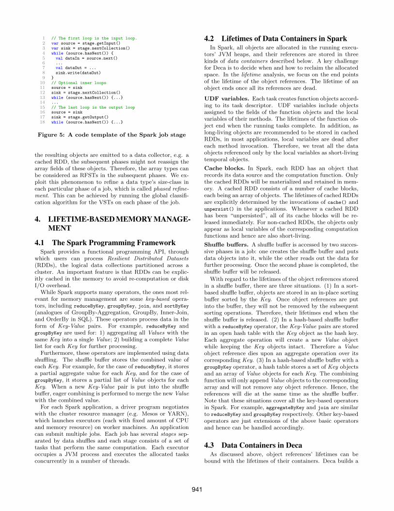
1 // The first loop is the input loop.2 var source = stage.getInput()3 var sink = stage.nextCollection()4 while (source.hasNext()) {5 val dataIn = source.next()6 ...7 val dataOut = ...8 sink.write(dataOut)9 }

10 // Optional inner loops11 source = sink12 sink = stage.nextCollection()13 while (source.hasNext()) {...}14 ...15 // The last loop is the output loop16 source = sink17 sink = stage.getOutput()18 while (source.hasNext()) {...}

Figure 5: A code template of the Spark job stage

the resulting objects are emitted to a data collector, e.g. acached RDD, the subsequent phases might not reassign thearray fields of these objects. Therefore, the array types canbe considered as RFSTs in the subsequent phases. We ex-ploit this phenomenon to refine a data type’s size-class ineach particular phase of a job, which is called phased refine-ment. This can be achieved by running the global classifi-cation algorithm for the VSTs on each phase of the job.

4. LIFETIME-BASED MEMORY MANAGE-MENT

4.1 The Spark Programming FrameworkSpark provides a functional programming API, through

which users can process Resilient Distributed Datasets(RDDs), the logical data collections partitioned across acluster. An important feature is that RDDs can be explic-itly cached in the memory to avoid re-computation or diskI/O overhead.

While Spark supports many operators, the ones most rel-evant for memory management are some key-based opera-tors, including reduceByKey, groupByKey, join, and sortByKey

(analogues of GroupBy-Aggregation, GroupBy, Inner-Join,and OrderBy in SQL). These operators process data in theform of Key-Value pairs. For example, reduceByKey andgroupByKey are used for: 1) aggregating all Values with thesame Key into a single Value; 2) building a complete Valuelist for each Key for further processing.

Furthermore, these operators are implemented using datashuffling. The shuffle buffer stores the combined value ofeach Key. For example, for the case of reduceByKey, it storesa partial aggregate value for each Key, and for the case ofgroupByKey, it stores a partial list of Value objects for eachKey. When a new Key-Value pair is put into the shufflebuffer, eager combining is performed to merge the new Valuewith the combined value.

For each Spark application, a driver program negotiateswith the cluster resource manager (e.g. Mesos or YARN),which launches executors (each with fixed amount of CPUand memory resource) on worker machines. An applicationcan submit multiple jobs. Each job has several stages sep-arated by data shuffles and each stage consists of a set oftasks that perform the same computation. Each executoroccupies a JVM process and executes the allocated tasksconcurrently in a number of threads.

4.2 Lifetimes of Data Containers in SparkIn Spark, all objects are allocated in the running execu-

tors’ JVM heaps, and their references are stored in threekinds of data containers described below. A key challengefor Deca is to decide when and how to reclaim the allocatedspace. In the lifetime analysis, we focus on the end pointsof the lifetime of the object references. The lifetime of anobject ends once all its references are dead.

UDF variables. Each task creates function objects accord-ing to its task descriptor. UDF variables include objectsassigned to the fields of the function objects and the localvariables of their methods. The lifetimes of the function ob-ject end when the running tasks complete. In addition, aslong-living objects are recommended to be stored in cachedRDDs, in most applications, local variables are dead aftereach method invocation. Therefore, we treat all the dataobjects referenced only by the local variables as short-livingtemporal objects.

Cache blocks. In Spark, each RDD has an object thatrecords its data source and the computation function. Onlythe cached RDDs will be materialized and retained in mem-ory. A cached RDD consists of a number of cache blocks,each being an array of objects. The lifetimes of cached RDDsare explicitly determined by the invocations of cache() andunpersist() in the applications. Whenever a cached RDDhas been “unpersisted”, all of its cache blocks will be re-leased immediately. For non-cached RDDs, the objects onlyappear as local variables of the corresponding computationfunctions and hence are also short-living.

Shuffle buffers. A shuffle buffer is accessed by two succes-sive phases in a job: one creates the shuffle buffer and putsdata objects into it, while the other reads out the data forfurther processing. Once the second phase is completed, theshuffle buffer will be released.

With regard to the lifetimes of the object references storedin a shuffle buffer, there are three situations. (1) In a sort-based shuffle buffer, objects are stored in an in-place sortingbuffer sorted by the Key. Once object references are putinto the buffer, they will not be removed by the subsequentsorting operations. Therefore, their lifetimes end when theshuffle buffer is released. (2) In a hash-based shuffle bufferwith a reduceByKey operator, the Key-Value pairs are storedin an open hash table with the Key object as the hash key.Each aggregate operation will create a new Value objectwhile keeping the Key objects intact. Therefore a Valueobject reference dies upon an aggregate operation over itscorresponding Key. (3) In a hash-based shuffle buffer with agroupByKey operator, a hash table stores a set of Key objectsand an array of Value objects for each Key. The combiningfunction will only append Value objects to the correspondingarray and will not remove any object reference. Hence, thereferences will die at the same time as the shuffle buffer.Note that these situations cover all the key-based operatorsin Spark. For example, aggregateByKey and join are similarto reduceByKey and groupByKey respectively. Other key-basedoperators are just extensions of the above basic operatorsand hence can be handled accordingly.

4.3 Data Containers in DecaAs discussed above, object references’ lifetimes can be

bound with the lifetimes of their containers. Deca builds a

941

page 0

79FB

FF3C

pointers

...

page 1

K V K

...

V

(a) Cache Block (b) Shuffle Buffer

page 0

page 1

...

K V

K V K V

page 2

Figure 6: Memory layouts of data containers

data dependent graph for each job stage by points-to anal-ysis [20] to produce the mapping relationships between allthe objects and their containers. Objects are identified byeither their creation statements if they are created in thecurrent stage, or their source cached blocks if they are readfrom cached blocks created by the previous stage.

However, an object can be assigned to multiple data con-tainers. For example, if objects are copies between two dif-ferent cached RDDs, then they can be bound to the cachedblocks of both RDDs. In such cases, we assign a sole pri-mary container as the owner of each data object. Othercontainers are treated as secondary containers. The objectownership is determined based on the following rules:

1. Cached RDDs and shuffle buffers have higher priorityof data ownership than UDF variables, simply due totheir longer expected lifetimes.

2. If there are objects assigned to multiple high-prioritycontainers in the same job stage, the container createdfirst in the stage execution will own these objects.

The rest of this subsection presents how data are orga-nized within the primary and secondary containers.

4.3.1 Memory Pages in DecaDeca uses unified byte arrays with a common fixed size as

logical memory pages to store the decomposed data objects.A page can be logically split into consecutive byte segments,one for each top-layer object. Each of such segment can befurther split into multiple segments, one for each lower-layerobject, and so on. The page size is chosen to ensure thatthere is only a moderate number of pages in each executor’sJVM heap so that the GC overhead is negligible. On theother hand, the page size should not be too large either, sothat there would not be a significant unused space in thelast page of a container.

For each data container, a group of pages are allocated tostore the objects it owns. Deca uses a page-info structureto maintain the metadata of each page group. The page-info of each page graph contains: 1) pages, a page arraystoring the references of all the allocated pages of this pagegroup; 2) endOffset, an integer storing the start offset ofthe unused part of the last page in this group; 3) curPageand curOffset, two integer values that store the progress ofsequentially scanning, or appending to, this page group.

4.3.2 Primary ContainerIn the following, we present how Deca stores objects in

the different types of primary containers. For brevity, weomit swapping data between memory and disks here. It isstraightforward to adapt to the cases with disk swapping fordata caching and shuffling (see [3]).

UDF variables. Deca does not decompose objects ownedby UDF variables. These objects do not incur significant

GC overheads, because: (1) the objects only referenced bylocal variables are short-living objects and they belong tothe young generation, which will be reclaimed by the cheapminor GCs; (2) the objects referenced by the function objectfields may be promoted to the part of old generation, butthe total number of these objects in a task is relatively smallin comparing to the big input dataset.

Cache blocks. Deca always decomposes the SFST or RFSTobjects and stores their raw data bytes in the page groupof a cache block, while keeps the VST objects intact. Fig-ure 6(a) shows the structure of a cache block of a cachedRDD, which contains decomposed objects.

A task can read objects from a decomposed cache blockcreated in a previous phase. If this task changes the data-sizes of these objects, Deca has to re-construct the objectsand release the original page group. To avoid thrashing,when such re-construction happens, Deca will not decom-pose these objects again even if they can be safely decom-posed in the subsequent phases.

Shuffle buffers. Figure 6(b) shows the structure of a shuf-fle buffer. Similar to cache blocks, data of an RFST or anSFST in a shuffle buffer will be decomposed into the shufflebuffer’s page group. However, unlike cached RDD, wheredata are accessed in a sequential manner, data in a shufflebuffer will be randomly accessed to perform sorting or hash-ing operations. Therefore, as illustrated on the left-handside of Figure 6(b), we use an array to store the pointers tothe keys and values within a page. The hashing and sortingoperations are performed on the pointer arrays. However,the pointer array can be avoided for a hash-based shufflebuffer with both the Key and the Value being of primitivetypes or SFSTs. This is because we can deduce the offsetsof the data within the page statically.

As we discussed in Section 4.2, for a hash-based shufflebuffer with a GroupBy-Aggregation computation, a com-bining operation would kill the old Value object and cre-ate a new one. Therefore, Value objects are not long-livingand frequent GC of these objects are generally unavoidable.However, if the Value object is of an SFST, then we canstill decompose it and whenever a new object is generatedby the combining operation, we can just reuse the page seg-ment occupied by the old object, because the old and thenew objects are of the same size. Doing this would save thefrequent GC caused by these temporary Value objects.

4.3.3 Secondary ContainerThere are common patterns of multiple data containers

sharing the same data objects in Spark programs, such as: 1)manipulating data objects in cache blocks or shuffle buffersthrough UDF variables; 2) copying objects between cachedRDDs; 3) immediately caching the output objects of shuf-fling; 4) immediately shuffling the objects of a cached RDD.

If a secondary container is UDF variables, it will be as-signed pointers to page segments in the page group of the ob-jects’ primary container. Otherwise, Deca stores data in thesecondary container according to the following two differentscenarios: (i) fully decomposable, where the objects can besafely decomposed in all the containers, and (ii) partiallydecomposable, where the objects cannot be decomposed inone or more containers.

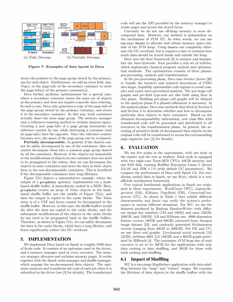
Fully decomposable. This scenario is illustrated in Fig-ure 7(a). To avoid copy-by-value, a secondary container only

942

···

page 0

···

page 1

Primary Secondary

···

page 2

depPage

page-infopage-info

···

page 0

page 1

···

(a) Fully Decomp.

j

2i 2i+1

Key

Shuffle Buffer

Array[AnyRef]

value

ArrayBuffer

Value Array[Integer]

value

...Cache Block

Array[byte]

lengthcountvalues ...

(b) Partially Decomp.

Figure 7: Examples of data layout in Deca

stores the pointers to the page group owned by the primary,one for each object. Furthermore, we add an extra field, dep-Pages, to the page-info of the secondary container to storethe page-info(s) of the primary container(s).

Deca further performs optimizations for a special case,where a secondary container stores the same set of objectsas the primary and does not require a specific data ordering.In such a case, Deca only generates a copy of the page-info ofthe page group owned by the primary container, and storesit in the secondary container. In this way, both containersactually share the same page group. The memory manageruses a reference-counting method to reclaim memory space.Creating a new page-info of a page group increments itsreference counter by one, while destroying a container (andits page-info) does the opposite. Once the reference counterbecomes zero, the space of the page group can be reclaimed.

Partially decomposable. In general, if the objects can-not be safely decomposed in one of the containers, then wecannot decompose them into a common page group sharedby all the containers. However, if the objects are immutableor the modifications of objects in one container does not needto be propagated to the others, then we can decompose theobjects in some containers and store the data in their objectform in the non-decomposable containers. This is beneficialif the decomposable containers have long lifetimes.

Figure 7(b) depicts a representative example, where theoutput of a groupByKey operator, implemented via a hash-based shuffle buffer, is immediately cached in a RDD. Here,groupByKey creates an array of Value objects in the hash-based shuffle buffer (see the middle of Figure 7(b)), andthen the output is copied to the cache blocks. The Valuearray is of a VST and hence cannot be decomposed in theshuffle buffer. However, in this case, the shuffle buffers woulddie after the data are copied to the cache blocks, and thesubsequent modifications of the objects in the cache blocksdo not need to be propagated back to the shuffle buffers.Therefore, as shown in Figure 7(b), we can safely decomposethe data in the cache blocks, which have a long lifetime, andhence significantly reduce the GC overhead.

5. IMPLEMENTATIONWe implement Deca based on Spark in roughly 6700 lines

of Scala code. It consists of an optimizer used in the driver,and a memory manager used in every executor. The mem-ory manager allocates and reclaims memory pages. It workstogether with the Spark cache manager and shuffle manager,which manage the un-decomposed data objects. The opti-mizer analyzes and transforms the code of each job when it issubmitted in the driver (see [3] for details). The transformed

code will use the API provided by the memory manager tocreate pages and access the stored bytes.

Currently we do not use off-heap memory to store de-composed data. However, our method is independent onthe mechanism of JVM GC. In other words, we can usesun.misc.Unsafe to allocate and release memory space out-side of the JVM heap. Using Unsafe can completely elimi-nate the GC overhead, but it requires a user to estimate howmuch data should be stored inside and outside the heap.

Deca uses the Soot framework [6] to analyze and manipu-late the Java bytecode. Soot provides a rich set of utilities,which implements classical program analysis and optimiza-tion methods. The optimization consists of three phases:pre-processing, analysis and transformation.

In the pre-processing phase, Deca uses iterator fusion [26]to bundle the iterative and isolated invocations of UDFsinto larger, hopefully optimizable code regions to avoid com-plex and costly inter-procedural analysis. The per-stage callgraphs and per-field type-sets are also built using Soot inthis phase. Building per-phase call graphs will be delayedto the analysis phase if a phased refinement is necessary. Inthe analysis phase, Deca uses methods described in Section 3and Section 4 to determine whether and how to decomposeparticular data objects in their containers. Based on theobtained decomposability information, new class files withtransformed code will be generated and distributed to allexecutors in the transformation phase. In general, the ac-cessing of primitive fields of decomposed data objects in theoriginal code will be transformed to access the correspondingpage segments (see [3] for details).

6. EVALUATIONWe use five nodes in the experiments, with one node as

the master and the rest as workers. Each node is equippedwith two eight-core Xeon-2670 CPUs, 64GB memory andone SAS disk, running RedHat Enterprise Linux 5 (kernel2.6.18) and JDK 1.7.0 (with default GC parameters). Wecompare the performance of Deca with Spark 1.6. For seri-alizing cached data in Spark, we use Kryo, which is a veryefficient serialization framework.

Five typical benchmark applications in Spark are evalu-ated in these experiments: WordCount (WC), LogisticRe-gression (LR), KMeans, PageRank (PR), ConnectedCom-ponent (CC). As shown in Table 1 they exhibit differentcharacteristics and hence can verify the system’s perfor-mance in various different situations. For WC, we use thedatasets produced by Hadoop RandomWriter with differ-ent unique key numbers (1M and 100M) and sizes (50GB,100GB, and 150GB). LR and KMeans use: 4096-dimensionfeature vectors (40GB and 80GB) extracted from Amazonimage dataset [23], and randomly generated 10-dimensionvectors (ranging from 40GB to 200GB). For PR and CC,we use three real graphs: LiveJournal social network [13](2GB), webbase-2001 [14] (30GB) and a 60GB graph gener-ated by HiBench [4]. The maximum JVM heap size of eachexecutor is set to be 30GB for the applications with onlydata caching or data shuffling, and 20GB for those withboth caching and shuffling.

6.1 Impact of ShufflingWC is a two-stage MapReduce application with data shuf-

fling between the “map” and “reduce” stages. We examinethe lifetimes of data objects in the shuffle buffers with the

943

Table 1: Applications used in the experimentsApplication Stages Jobs Cache Shuffle

WC two single non aggregatedLR single multiple static non

KMeans two multiple static aggregatedPRCC

multiple multiple staticgrouped

aggregated

1

100

10000

1x106

1x108

1x1010

0 500 1000 1500 2000 0

10

20

30

40

50

60

70

80

90

100

Nu

mb

er o

f O

bje

cts

Tim

e o

f G

C(s

)

Time(s)

Spark-Tuple2Spark-GC

Deca-Tuple2Deca-GC

(a) WC lifetime

0

1

2

3

4

5

6

50GB 100GB 150GB 50GB 100GB 150GB

Ex

ecu

tio

n T

ime

(10

00

s)

Data Size / Key Size

Spark-execDeca-exec

0

1

2

3

4

5

6

10M 100M

Ex

ecu

tio

n T

ime

(10

00

s)

Data Size / Key Size

(b) WC exec

Figure 8: Results of shuffling-only WC

smallest dataset. We periodically record the alive numberof objects and the GC time with JProfiler 9.0. The re-sult is shown in Figure 8(a). WC uses a hash-based shufflebuffer to perform eager aggregation, which is implementedin Tuple2. The number of Tuple2 objects, which fluctuatesduring the execution, can indicate the number of objects inshuffle buffers. While the number of Tuple2 is also largein ”map” stage but decreases in shuffle in Deca. GCs aretriggered frequently to release the space occupied by thetemporary objects in the shuffle buffers.

To avoid such frequent GC operations, Deca reuses thespace occupied by the partially-aggregated Value for eachKey in the shuffle buffer. Figure 8(b) compares the execu-tion times of Deca and Spark. In all cases, Deca can reducethe execution time by 10%–58%. One could also see that theperformance improvement increases with more number ofkeys. This is because the size of a hash-based shuffle bufferwith eager aggregation mainly depends on the number ofkeys. The reduction of GC overhead would become moreprominent with a larger number of keys. Furthermore, sinceDeca stores the objects in the shuffle buffer as byte arrays,it also saves the cost of data (de-)serialization by directlyoutputting the raw bytes.

6.2 Impact of CachingLR and KMeans are representative machine learning ap-

plications that perform iterative computations. Both ofthem first load and cache the training dataset into memory,then iteratively update the model until the pre-defined con-vergence condition is met. In our experiments, we only run30 iterations. We do not account for the time to load thetraining dataset, because the iterative computation domi-nates the execution time, especially considering that theseapplications can run up to hundreds of iterations in a pro-duction environment. We set 90% of the available memoryto be used for data caching.

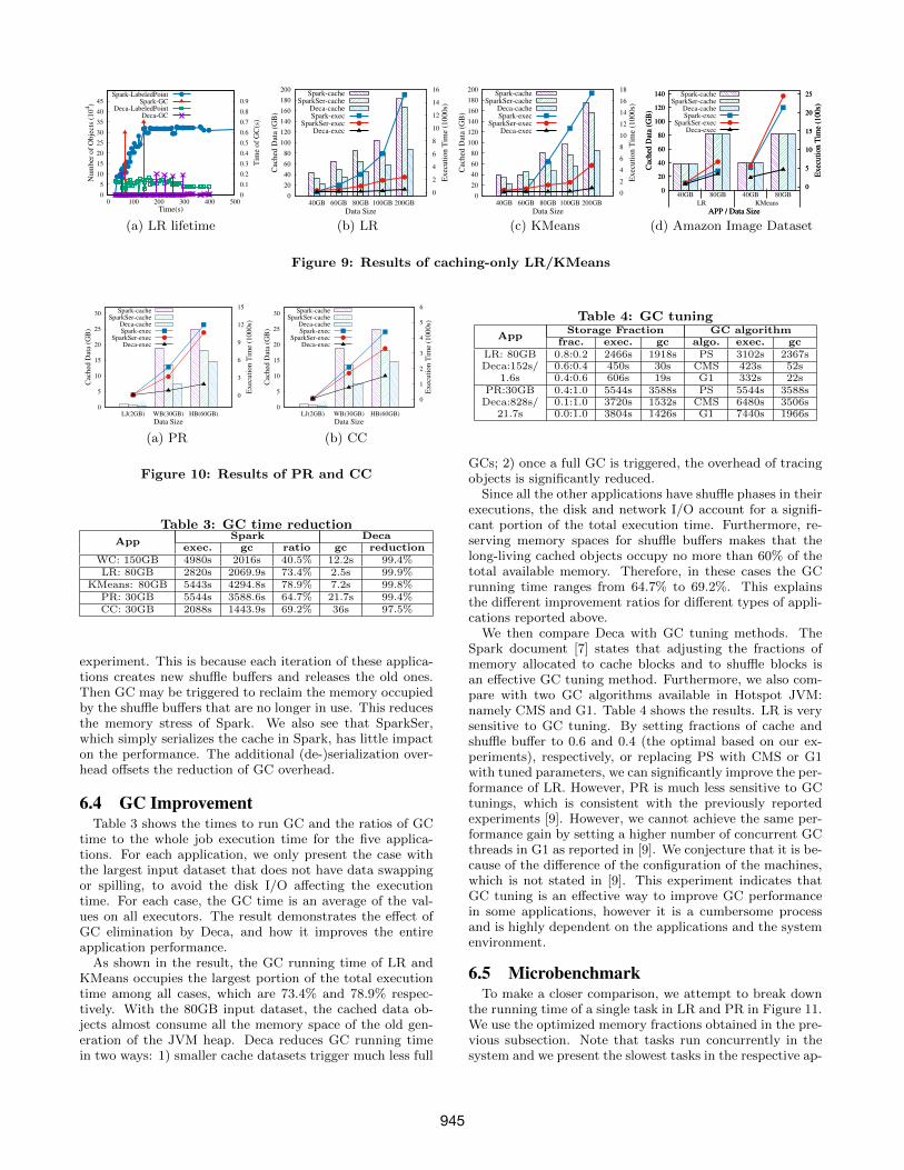
We first examine the lifetimes of data objects in cacheRDDs for LR using the 40GB dataset. The result is shownin Figure 9(a). We find that the number of objects is ratherstable throughout the execution in Spark, but full GCs havebeen triggered several times in vain (the peaks of the GC

time curve). This is because most objects are long-living andhence their space cannot be reclaimed. While these objectsare less in Deca because they are transformed to bytes afterbeing read from the HDFS. Some objects still live in oldgeneration of JVM heap because no full GC is active.

By grouping massive objects with the same lifetime intoa few byte arrays, Deca can effectively eliminate the GCproblem of repeatedly scanning alive data objects for theirliveness. Figure 9(b) and Figure 9(c) show the executiontimes of LR and KMeans for both Deca and Spark. Herewe also examine the cases using Kryo to serialize the cacheddata in Spark, which is denoted as “SparkSer” in the figures.

For the 40GB and 60GB datasets, the improvement ismoderate and can be mainly attributed to the elimination ofobject creation and minor GCs. In these cases, the memoryis sufficient to store the temporary objects, and hence fullGC is rarely triggered. Furthermore, serializing the cacheddata also helps reducing the GC time. Therefore, with the40GB dataset, SparkSer outperforms Spark by reducing theGC overhead. However, for larger datasets, the overheadof data (de-)serialization cannot pay off the reduced GCoverhead. Therefore, simply serializing the cached data isnot a robust solution.

For the three larger datasets the improvement is moresignificant. The speedups of Deca are ranging from 16x to41.6x. In these datasets, the long-living objects consumealmost all available memory space, and therefore full GCsare frequently triggered, which just repeatedly and unavail-ingly trace the cached data objects in the old generationof the JVM heap. With the 100GB and 200GB datasets,the additional disk I/O costs of cache swapping also prolongthe execution times of Spark. Deca keeps a smaller memoryfootprint of cached data and swap smaller portion of datato the disks.

We also conduct the experiments on a real dataset, Ama-zon image dataset with 4096 dimensions. Figure 9(d) showsthe speedups achieved by Deca are ranging from 1.2x to5.3x. With such a high dimensional dataset, the size of ob-ject headers becomes negligible and therefore, the sizes ofthe cached data of Spark and Deca are nearly identical.

6.3 Impact of Mixed Shuffling and Caching

Table 2: Graph datasets used in PR and CCGraph LiveJournal (LJ) WebBase (WB) HiBench (HB)Vertices 4.8M 118M 602MEdges 68M 1B 2B

Data Size 2GB 30GB 60GB

PR and CC are representative iterative graph computa-tions. Both of them use groupByKey to transform the edge listto the adjacency lists, and then cache the resulting data. Weuse three datasets with different edge numbers and vertexnumbers as shown in Table 2. We set 40% and 100% of theavailable heap space for caching and shuffling respectively.Edges will be cached during all iterations, and shuffling isused in every iteration to aggregate messages for each targetvertex. We run 10 iterations in all the experiments.

Figure 10(a) and Figure 10(b) show the execution times ofPR and CC for both Spark and Deca. The speedups of Decaare ranging from 1.1x to 6.4x, which again can be attributedto the reduction of GC overhead and shuffle serializationoverhead. However, it is less dramatic than the previous

944

0

5

10

15

20

25

30

35

40

45

0 100 200 300 400 500 0

0.1

0.2

0.3

0.4

0.5

0.6

0.7

0.8

0.9

Num

ber

of

Obje

cts

(10

4)

Tim

e of

GC

(s)

Time(s)

Spark-LabeledPointSpark-GC

Deca-LabeledPointDeca-GC

(a) LR lifetime

0

20

40

60

80

100

120

140

160

180

200

40GB 60GB 80GB 100GB 200GB

0

2

4

6

8

10

12

14

16

Cac

hed

Dat

a (G

B)

Exec

uti

on T

ime

(1000s)

Data Size

Spark-cacheSparkSer-cache

Deca-cacheSpark-exec

SparkSer-execDeca-exec

(b) LR

0

20

40

60

80

100

120

140

160

180

200

40GB 60GB 80GB 100GB 200GB

0

2

4

6

8

10

12

14

16

18

Cac

hed

Dat

a (G

B)

Exec

uti

on T

ime

(1000s)

Data Size

Spark-cacheSparkSer-cache

Deca-cacheSpark-exec

SparkSer-execDeca-exec

(c) KMeans

0

20

40

60

80

100

120

140

40GB 80GB 40GB 80GB

0

5

10

15

20

25

Cac

hed

Dat

a (G

B)

Exec

uti

on T

ime

(100s)

APP / Data Size

Spark-cacheSparkSer-cache

Deca-cacheSpark-exec

SparkSer-execDeca-exec

0

20

40

60

80

100

120

140

LR KMeans

0

5

10

15

20

25

Cac

hed

Dat

a (G

B)

Exec

uti

on T

ime

(100s)

APP / Data Size

(d) Amazon Image Dataset

Figure 9: Results of caching-only LR/KMeans

0

5

10

15

20

25

30

LJ(2GB) WB(30GB) HB(60GB)

0

3

6

9

12

15

Cac

hed

Dat

a (G

B)

Ex

ecu

tio

n T

ime

(10

00

s)

Data Size

Spark-cacheSparkSer-cache

Deca-cacheSpark-exec

SparkSer-execDeca-exec

(a) PR

0

5

10

15

20

25

30

LJ(2GB) WB(30GB) HB(60GB)

0

1

2

3

4

5

6

Cac

hed

Dat

a (G

B)

Ex

ecu

tio

n T

ime

(10

00

s)Data Size

Spark-cacheSparkSer-cache

Deca-cacheSpark-exec

SparkSer-execDeca-exec

(b) CC

Figure 10: Results of PR and CC

Table 3: GC time reductionApp

Spark Decaexec. gc ratio gc reduction

WC: 150GB 4980s 2016s 40.5% 12.2s 99.4%LR: 80GB 2820s 2069.9s 73.4% 2.5s 99.9%

KMeans: 80GB 5443s 4294.8s 78.9% 7.2s 99.8%PR: 30GB 5544s 3588.6s 64.7% 21.7s 99.4%CC: 30GB 2088s 1443.9s 69.2% 36s 97.5%

experiment. This is because each iteration of these applica-tions creates new shuffle buffers and releases the old ones.Then GC may be triggered to reclaim the memory occupiedby the shuffle buffers that are no longer in use. This reducesthe memory stress of Spark. We also see that SparkSer,which simply serializes the cache in Spark, has little impacton the performance. The additional (de-)serialization over-head offsets the reduction of GC overhead.

6.4 GC ImprovementTable 3 shows the times to run GC and the ratios of GC

time to the whole job execution time for the five applica-tions. For each application, we only present the case withthe largest input dataset that does not have data swappingor spilling, to avoid the disk I/O affecting the executiontime. For each case, the GC time is an average of the val-ues on all executors. The result demonstrates the effect ofGC elimination by Deca, and how it improves the entireapplication performance.

As shown in the result, the GC running time of LR andKMeans occupies the largest portion of the total executiontime among all cases, which are 73.4% and 78.9% respec-tively. With the 80GB input dataset, the cached data ob-jects almost consume all the memory space of the old gen-eration of the JVM heap. Deca reduces GC running timein two ways: 1) smaller cache datasets trigger much less full

Table 4: GC tuning

AppStorage Fraction GC algorithm

frac. exec. gc algo. exec. gcLR: 80GB 0.8:0.2 2466s 1918s PS 3102s 2367sDeca:152s/ 0.6:0.4 450s 30s CMS 423s 52s

1.6s 0.4:0.6 606s 19s G1 332s 22sPR:30GB 0.4:1.0 5544s 3588s PS 5544s 3588sDeca:828s/ 0.1:1.0 3720s 1532s CMS 6480s 3506s

21.7s 0.0:1.0 3804s 1426s G1 7440s 1966s

GCs; 2) once a full GC is triggered, the overhead of tracingobjects is significantly reduced.

Since all the other applications have shuffle phases in theirexecutions, the disk and network I/O account for a signifi-cant portion of the total execution time. Furthermore, re-serving memory spaces for shuffle buffers makes that thelong-living cached objects occupy no more than 60% of thetotal available memory. Therefore, in these cases the GCrunning time ranges from 64.7% to 69.2%. This explainsthe different improvement ratios for different types of appli-cations reported above.

We then compare Deca with GC tuning methods. TheSpark document [7] states that adjusting the fractions ofmemory allocated to cache blocks and to shuffle blocks isan effective GC tuning method. Furthermore, we also com-pare with two GC algorithms available in Hotspot JVM:namely CMS and G1. Table 4 shows the results. LR is verysensitive to GC tuning. By setting fractions of cache andshuffle buffer to 0.6 and 0.4 (the optimal based on our ex-periments), respectively, or replacing PS with CMS or G1with tuned parameters, we can significantly improve the per-formance of LR. However, PR is much less sensitive to GCtunings, which is consistent with the previously reportedexperiments [9]. However, we cannot achieve the same per-formance gain by setting a higher number of concurrent GCthreads in G1 as reported in [9]. We conjecture that it is be-cause of the difference of the configuration of the machines,which is not stated in [9]. This experiment indicates thatGC tuning is an effective way to improve GC performancein some applications, however it is a cumbersome processand is highly dependent on the applications and the systemenvironment.

6.5 MicrobenchmarkTo make a closer comparison, we attempt to break down

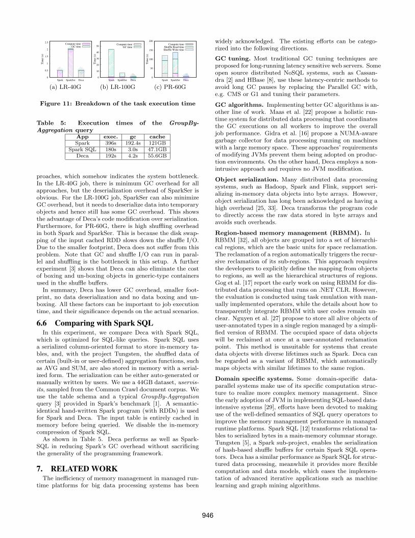
the running time of a single task in LR and PR in Figure 11.We use the optimized memory fractions obtained in the pre-vious subsection. Note that tasks run concurrently in thesystem and we present the slowest tasks in the respective ap-

945

0

0.5

1

1.5

2

2.5

Spark SparkSer Deca

Tim

e (s

)Compute time

GC time

(a) LR-40G

0

10

20

30

40

50

Spark SparkSer Deca

Tim

e (s

)

Compute timeGC time

(b) LR-100G

0

50

100

150

200

Spark SparkSer Deca

Tim

e (s

)

Compute timeShuffle Read timeShuffle Write time

(c) PR-60G

Figure 11: Breakdown of the task execution time

Table 5: Execution times of the GroupBy-Aggregation query

App exec. gc cacheSpark 396s 192.4s 121GB

Spark SQL 180s 3.0s 47.1GBDeca 192s 4.2s 55.6GB

proaches, which somehow indicates the system bottleneck.In the LR-40G job, there is minimum GC overhead for allapproaches, but the deserialization overhead of SparkSer isobvious. For the LR-100G job, SparkSer can also minimizeGC overhead, but it needs to deserialize data into temporaryobjects and hence still has some GC overhead. This showsthe advantage of Deca’s code modification over serialization.Furthermore, for PR-60G, there is high shuffling overheadin both Spark and SparkSer. This is because the disk swap-ping of the input cached RDD slows down the shuffle I/O.Due to the smaller footprint, Deca does not suffer from thisproblem. Note that GC and shuffle I/O can run in paral-lel and shuffling is the bottleneck in this setup. A furtherexperiment [3] shows that Deca can also eliminate the costof boxing and un-boxing objects in generic-type containersused in the shuffle buffers.

In summary, Deca has lower GC overhead, smaller foot-print, no data deserialization and no data boxing and un-boxing. All these factors can be important to job executiontime, and their significance depends on the actual scenarios.

6.6 Comparing with Spark SQLIn this experiment, we compare Deca with Spark SQL,

which is optimized for SQL-like queries. Spark SQL usesa serialized column-oriented format to store in-memory ta-bles, and, with the project Tungsten, the shuffled data ofcertain (built-in or user-defined) aggregation functions, suchas AVG and SUM, are also stored in memory with a serial-ized form. The serialization can be either auto-generated ormanually written by users. We use a 44GB dataset, uservis-its, sampled from the Common Crawl document corpus. Weuse the table schema and a typical GroupBy-Aggregationquery [3] provided in Spark’s benchmark [1]. A semantic-identical hand-written Spark program (with RDDs) is usedfor Spark and Deca. The input table is entirely cached inmemory before being queried. We disable the in-memorycompression of Spark SQL.

As shown in Table 5. Deca performs as well as Spark-SQL in reducing Spark’s GC overhead without sacrificingthe generality of the programming framework.

7. RELATED WORKThe inefficiency of memory management in managed run-

time platforms for big data processing systems has been

widely acknowledged. The existing efforts can be catego-rized into the following directions.

GC tuning. Most traditional GC tuning techniques areproposed for long-running latency sensitive web servers. Someopen source distributed NoSQL systems, such as Cassan-dra [2] and HBase [8], use these latency-centric methods toavoid long GC pauses by replacing the Parallel GC with,e.g. CMS or G1 and tuning their parameters.

GC algorithms. Implementing better GC algorithms is an-other line of work. Maas et al. [22] propose a holistic run-time system for distributed data processing that coordinatesthe GC executions on all workers to improve the overalljob performance. Gidra et al. [16] propose a NUMA-awaregarbage collector for data processing running on machineswith a large memory space. These approaches’ requirementsof modifying JVMs prevent them being adopted on produc-tion environments. On the other hand, Deca employs a non-intrusive approach and requires no JVM modification.

Object serialization. Many distributed data processingsystems, such as Hadoop, Spark and Flink, support seri-alizing in-memory data objects into byte arrays. However,object serialization has long been acknowledged as having ahigh overhead [25, 33]. Deca transforms the program codeto directly access the raw data stored in byte arrays andavoids such overheads.

Region-based memory management (RBMM). InRBMM [32], all objects are grouped into a set of hierarchi-cal regions, which are the basic units for space reclamation.The reclamation of a region automatically triggers the recur-sive reclamation of its sub-regions. This approach requiresthe developers to explicitly define the mapping from objectsto regions, as well as the hierarchical structures of regions.Gog et al. [17] report the early work on using RBMM for dis-tributed data processing that runs on .NET CLR. However,the evaluation is conducted using task emulation with man-ually implemented operators, while the details about how totransparently integrate RBMM with user codes remain un-clear. Nguyen et al. [27] propose to store all alive objects ofuser-annotated types in a single region managed by a simpli-fied version of RBMM. The occupied space of data objectswill be reclaimed at once at a user-annotated reclamationpoint. This method is unsuitable for systems that createdata objects with diverse lifetimes such as Spark. Deca canbe regarded as a variant of RBMM, which automaticallymaps objects with similar lifetimes to the same region.

Domain specific systems. Some domain-specific data-parallel systems make use of its specific computation struc-ture to realize more complex memory management. Sincethe early adoption of JVM in implementing SQL-based data-intensive systems [29], efforts have been devoted to makinguse of the well-defined semantics of SQL query operators toimprove the memory management performance in managedruntime platforms. Spark SQL [12] transforms relational ta-bles to serialized bytes in a main-memory columnar storage.Tungsten [5], a Spark sub-project, enables the serializationof hash-based shuffle buffers for certain Spark SQL opera-tors. Deca has a similar performance as Spark SQL for struc-tured data processing, meanwhile it provides more flexiblecomputation and data models, which eases the implemen-tation of advanced iterative applications such as machinelearning and graph mining algorithms.

946

8. CONCLUSIONIn this paper, we identify that GC overhead in distributed

data processing systems is unnecessarily high. By presentingDeca’s techniques of analyzing the variability of object sizesand safely decomposing objects in different containers, weshow that it is possible to develop a general and efficientlifetime-based memory manager for such systems to largelyeliminate the high GC overhead. The experiment resultsshow that Deca can significantly reduce Spark’s applicationrunning time for various cases without losing the generalityof its programming framework. To take advantage of Deca’soptimization, users should not create a large number of long-living VST objects, which cannot be safely decomposed.

Acknowledgments. We thank Beng Chin Ooi, Xipeng Shenand Bingsheng He for their valuable comments. This pa-per is partly supported by two grants from the NSFC (No.61433019 and No. 61370104), a grant from the InternationalScience and Technology Cooperation Program of China (No.2015DFE12860), a grant from the National 863 Hi-Tech Re-search and Development Program (No. 2014AA01A301).

9. REFERENCES[1] Big data benchmark. http://tinyurl.com/qg93r43.

[2] Cassandra GC tuning. http://tinyurl.com/5u58mzc.

[3] Full version. https://arxiv.org/abs/1602.01959.

[4] HiBench suite. http://tinyurl.com/cns79vt.

[5] Project Tungsten. http://tinyurl.com/mzw7hew.

[6] Soot framework. http://sable.github.io/soot/.

[7] Spark GC tuning. http://tinyurl.com/hzf3gqm.

[8] Tuning Java garbage collection for HBase.http://tinyurl.com/j5hsd3x.

[9] Tuning Java garbage collection for Spark applications.http://tinyurl.com/pd8kkau.

[10] G. Anantharayanan, S. Kandula, A. Greenberg,I. Stoica, Y. Lu, B. Saha, and E. Harris. Reining inthe outliers in MapReduce clusters using Mantri. InOSDI, pages 265–278, 2010.

[11] E. Anderson and J. Tucek. Efficiency matters! InHotStorage, pages 40–45, 2009.

[12] M. Armbrust, R. S. Xin, C. Lian, Y. Huai, D. Liu,J. K. Bradley, X. Meng, T. Kaftan, M. J. Franklin,A. Ghodsi, and M. Zaharia. Spark SQL: Relationaldata processing in Spark. In SIGMOD, pages1383–1394, 2015.

[13] L. Backstrom, D. Huttenlocher, J. Kleinberg, andX. Lan. Group formation in large social networks:Membership, growth, and evolution. In KDD, pages44–54, 2006.

[14] P. Boldi and S. Vigna. The WebGraph framework I:Compression techniques. In WWW, pages 595–602,2004.

[15] Y. Bu, V. Borkar, G. Xu, and M. J. Carey. Abloat-aware design for big data applications. In ISMM,pages 119–130, 2013.

[16] L. Gidra, G. Thomas, J. Sopena, M. Shapiro, andN. Nguyen. NumaGiC: a garbage collector for big dataon big NUMA machines. In ASPLOS, pages 661–673,2015.

[17] I. Gog, J. Giceva, M. Schwarzkopf, K. Vaswani,D. Vytiniotis, G. Ramalingan, M. Costa, D. Murray,S. Hand, and M. Isard. Broom: sweeping out garbage

collection from big data systems. In HotOS, pages 2–2,2015.

[18] M. Isard, V. Prabhakaran, J. Currey, U. Wieder,K. Talwar, and A. Goldberg. Quincy: Fair schedulingfor distributed computing clusters. In SOSP, pages261–276, 2009.

[19] R. Jones, A. Hosking, and E. Moss. The garbagecollection handbook: the art of automatic memorymanagement. Chapman and Hall/CRC, 2011.

[20] O. Lhotak and L. Hendren. Scaling Java points-toanalysis using SPARK. In CC, pages 153–169, 2003.

[21] B. Li, E. Mazur, Y. Diao, A. McGregor, andP. Shenoy. A platform for scalable one-pass analyticsusing MapReduce. In SIGMOD, pages 985–996, 2011.

[22] M. Maas, T. Harris, K. A. c, and J. Kubiatowicz.Trash day: Coordinating garbage collection indistributed systems. In HotOS, pages 1–1, 2015.

[23] J. McAuley, C. Targett, Q. Shi, and A. van denHengel. Image-based recommendations on styles andsubstitutes. In SIGIR, pages 43–52, 2015.

[24] F. McSherry, M. Isard, and D. G. Murray. Scalability!but at what COST? In HotOS, pages 14–14, 2015.

[25] H. Miller, P. Haller, E. Burmako, and M. Odersky.Instant pickles: Generating object-oriented picklercombinators for fast and extensible serialization. InOOPSLA, pages 183–202, 2013.

[26] D. G. Murray, M. Isard, and Y. Yu. Steno: Automaticoptimization of declarative queries. In PLDI, pages121–131, 2011.

[27] K. Nguyen, K. Wang, Y. Bu, L. Fang, J. Hu, andG. Xu. FACADE: A compiler and runtime for(almost) object-bounded big data applications. InASPLOS, pages 675–690, 2015.

[28] R. Power and J. Li. Piccolo: Building fast, distributedprograms with partitioned tables. In OSDI, pages293–306, 2010.

[29] M. A. Shah, S. Madden, M. J. Franklin, and J. M.Hellerstein. Java support for data-intensive systems:Experiences building the telegraph dataflow system.SIGMOD Rec., 30(4):103–114, 2001.

[30] J. Shi, Y. Qiu, U. F. Minhas, L. Jiao, C. Wang,B. Reinwald, and F. Ozcan. Clash of the titans:MapReduce vs. Spark for large scale data analytics.PVLDB, 8(13):2110–2121, 2015.

[31] A. Shinnar, D. Cunningham, B. Herta, andV. Saraswat. M3R: Increased performance forin-memory Hadoop jobs. PVLDB, 5(12):1736–1747,2012.

[32] M. Tofte and J.-P. Talpin. Region-based memorymanagement. Inf. Comput., 132(2):109–176, 1997.

[33] M. Welsh and D. Culler. Jaguar: enabling efficientcommunication and I/O in Java. Concurrency -Practice and Experience, 12(7):519–538, 2000.

[34] M. Zaharia, M. Chowdhury, T. Das, A. Dave, J. Ma,M. McCauley, M. J. Franklin, S. Shenker, andI. Stoica. Resilient distributed datasets: Afault-tolerant abstraction for in-memory clustercomputing. In NSDI, pages 2–2, 2012.

[35] M. Zaharia, A. Konwinski, A. D. Joseph, R. Katz, andI. Stoica. Improving MapReduce performance inheterogeneous environments. In OSDI, pages 29–42,2008.

947