LIFE HISTORY, ABUNDANCE, AND DISTRIBUTION OF THE SPOTTED

LIFE HISTORY, ABUNDANCE, AND DISTRIBUTION

OF THE SPOTTED RATFISH, Hydrolagus colliei

A Thesis

Presented to

The Faculty of Moss Landing Marine Laboratories

And the Institute of Earth Systems Science and Policy

California State University, Monterey Bay

In Partial Fulfillment

Of the Requirements for the Degree

Master of Science

In Marine Science

By

Lewis Abraham Kamuela Barnett

June 2008

i

© 2008 Lewis Abraham Kamuela Barnett

ALL RIGHTS RESERVED

ii

APPROVED FOR THE DEPARTMENT OF MARINE SCIENCE

________________________________________________ Dr. Gregor M. Cailliet, Advisor Moss Landing Marine Laboratories ________________________________________________ Dr. David A. Ebert Moss Landing Marine Laboratories Pacific Shark Research Center ________________________________________________ Dr. James T. Harvey Moss Landing Marine Laboratories ________________________________________________ Dr. Enric Cortés NOAA Fisheries, Southeast Fisheries Science Center APPROVED FOR THE UNIVERSITY ________________________________________________

iii

LIFE HISTORY, ABUNDANCE, AND DISTRIBUTION OF THE SPOTTED RATFISH, Hydrolagus colliei

Lewis Abraham Kamuela Barnett California State University, Monterey Bay

2008 Size at maturity, fecundity, reproductive periodicity, distribution, and abundance were

estimated for the spotted ratfish, Hydrolagus colliei, off the coast of California, Oregon,

and Washington (USA). Skeletal muscle concentrations of the steroid hormones

testosterone (T) and estradiol (E2) predicted similar, but slightly smaller sizes at maturity

than morphological criteria. Stage of maturity for males was estimated identically using

internal organs or external secondary sexual characters, thus allowing non-lethal maturity

assessments. Peak parturition occurred from May through October, with increased

concentrations of E2 and progesterone (P4) in skeletal muscle of females correlating with

ovarian recrudescence during November through February. Extrapolation of the

hypothesized 6 to 8 mo egg-laying season to observed mean parturition rates of captive

specimens yielded an estimated annual fecundity of 19.5 to 28.9 egg cases. Differences

in fecundity among higher taxonomic classifications of chondrichthyans were detected,

with chimaeriform fishes more fecund than myliobatiform, squaliform, and rhinobatiform

fishes. Delta-lognormal generalized linear models (GLMs) and cluster analysis indicated

the presence of two distinct stocks of H. colliei on the U.S. West Coast. Abundance of

the continental slope, and northern continental shelf and upper slope populations did not

vary between 1977 and 1995, but increased from 1995 to 2006. Abundance trends in the

southern shelf and upper slope region were not as straightforward, with increasing

abundance from 1977 to 1986, and lesser abundance thereafter, with the exception of an

iv

increase between 1992 and 1995. Although the life history, movement patterns, and

aggregative behavior of H. colliei indicated that it may be vulnerable to population

depletion by excess fisheries mortality, temporal abundance trends indicated that their

population size has increased significantly within the last decade. The paradigm that all

chondrichthyans are particularly susceptible to exploitation, therefore, may not apply to

chimaeroids. The hypothesis that the dorsal-fin spine of H. colliei is a reliable structure

for age estimation was tested by analyzing growth characteristics and imageing with

polarized light microscopy and micro-computed tomography. Variation among

individuals in the relationship between spine width and distance from the spine tip

indicated the technique of transverse sectioning may impart imprecision and bias to age

estimates. The number of growth band pairs observed by light microscopy in the inner

dentine layer was not a good predictor of body size. Mineral density gradients, indicative

of growth zones, were not observed in the H. colliei dorsal-fin spine, but were present in

hard parts used for age determination of the Patagonian toothfish (Dissostichus

eleginoides), roughtail skate (Bathyraja trachura), and spiny dogfish (Squalus

acanthias). The absence of mineral density gradients in the dorsal-fin spine of H. colliei

decreases the likelihood that the bands observed by light microscopy represent a record

of growth with consistent periodicity.

v

Acknowledgments

I thank my advisor Gregor Cailliet and co-advisor David Ebert for their great

assistance, guidance, and support. Additional thanks to my colleagues Wade Smith and

Joe Bizzarro for their superb advice and the wealth of knowledge and experience they

readily give. Committee members Jim Harvey and Enric Cortés provided many helpful

comments, improving my writing and synthesis skills. Mike Graham instigated many

intriguing scientific discussions, and was always available for questions at a moment’s

notice. Jason Cope (NOAA Fisheries, Northwest Fisheries Science Center, Seattle

Laboratory) and E.J. Dick (NOAA Fisheries, Southwest Fisheries Science Center, Santa

Cruz Laboratory) offered unparalleled assistance toward my education in generalized

linear modelling.

This project was made possible by cooperation and assistance in sample

collection provided by the NOAA Fisheries, Northwest Fishery Science Center,

especially Keith Bosley, Victor Simon, Erica Fruh, Melanie Johnson, and Beth Horness;

Mark Zimmermann of the NOAA Fisheries, Alaska Fisheries Science Center; Allen

Cramer, Sylvia Pauly, Kristen Green, and Jon Cusick of the West Coast Groundfish

Observer Program (a cooperative effort between NOAA Fisheries, Pacific States Marine

Fisheries Commission, and the states of Washington, Oregon, and California); Don

Pearson, Kevin Stierhoff, and Josh Bauman from the NOAA Fisheries, Southwest

Fisheries Science Center, Santa Cruz Laboratory; and Lee Bradford, Kurt Brown, and

Jason Felton of the R/V John H. Martin. Gilbert Van Dykhuisen (formerly of the

Monterey Bay Aquarium) graciously provided meticulously-collected data on the captive

vi

mating and spawning of spotted ratfish. Dan Howard (NOAA Fisheries, Cordell Bank

National Marine Sanctuary) stimulated several interesting discussions and eagerly

supplied submersible data, and spotted ratfish coffee mugs.

Special thanks to my colleagues in the ichthyology laboratory at MLML

(especially Aaron Carlisle, Chris Rinewalt, Tonatiuh Trejo, Matt Levey, Daniele

Ardizzone, Ashley Greenley, Simon Brown, Shaara Ainsley, Diane Haas, Ashley Neway,

Jasmine Fry, Cassandra Brooks, Kristen Green, and Mariah Boyle), for thoughtful

discussions, dissection assistance, entertainment on protracted van rides, laughter, and

foosball matches. I’m extremely appreciative of the Moss Landing Marine Labs

(MLML) front office staff, particularly Toni Fitzwater, Donna Kline, Kenneth Coale, and

John Machado. Thanks to Joan Parker and the library staff (especially Laurie Hall,

Shaara Ainsley, Rosemary Romero, Simon Brown, and Ashley Neway) for procuring

obscure documents at my request, and not hassling me too much when I tried to

interlibrary loan items that were available within our own confines. My sanity owes its

continued existence to my friends, most notably Alison Myers, Chris Scianni, Phil Hoos,

Ronnie Hoos, Charlie Endris, Jon Walsh, Berkeley Kauffman, and Cori Gibble. Without

these people distracting me from the rigors of graduate school, I would have burned out

much earlier, yet likely graduated sooner. I’m incredibly grateful for the emotional

support, patience, and love given by my girlfriend, Joëlle. She has kept my mind open,

and her influence has stoked my appreciation of so many things in life.

I owe my values, sense of humor, and love for the outdoors to my parents, Dave

and Barbara. Any and all of my successes in life can be attributed to my upbringing.

This work is dedicated to my mother, for teaching me the joys of reading and the nuances

vii

of caring. Thanks to my brother, Rabinder, for continuing to dispense brotherly advice,

despite my resistence to follow much of it. To the rest of my family, Norm, Rita, Jean,

Gail, Al, Jan, Mike, Deb, Greg, Zach, Chloë, Polly, Emily, Laurie, Paul, Susan,

Madeline, Lola, Paloma, Chris, and Miki, my sincere gratitude for being so loving, close,

and supportive.

This study was supported by funds from NOAA/NMFS to the National Shark

Research Consortium, Pacific Shark Research Center, and in part by the National Sea

Grant College Program of the U.S. Department of Commerce’s National Oceanic and

Atmospheric Administration under NOAA Grant no. NA04OAR4170038, project

number R/F-199, through the California Sea Grant College Program and in part by the

California State Resources Agency. Other funding was acquired from the Dr. Earl H.

Myers and Ethel M. Myers Oceanographic and Marine Biology Trust; Western Division

of the American Fisheries Society Eugene Maughan Graduate Student Scholarship;

David and Lucile Packard Research and Travel Award; John H. Martin Scholarship; San

Jose State University Professional Development Awards; Kim Peppard Memorial

Scholarship; and a PADI Foundation Grant.

viii

Table of Contents

List of Tables…………………………………………………………………………….xii

List of Figures…………………………………………………………………………...xiii

List of Appendices……………………………………………………………………..xviii

Chapter 1: Maturity, fecundity, and reproductive cycle.………………………...………..1

Introduction………………………………………………………………………………..2

Materials and Methods…………………………………………………………………….5

Reproductive Status……………………………………………………………….9

Reproductive Seasonality………………………………………………………...11

Results……………………………………………………………………………………14

Maturity…………………………………………………………………………..15

Effects of differing sample collection methods………………………………….17


Fecundity…………………………………………………………………………20

Discussion………………………………………………………………………………..21

Maturity…………………………………………………………………………..21


Fecundity…………………………………………………………………………28

Literature Cited…………………………………………………………………………..33

Tables…………………………………………………………………………………….51

Figures……………………………………………………………………………………56

ix

Chapter 2: Abundance and distribution………………………………………………….78

Introduction………………………………………………………………………………79

Materials and Methods…………………………………………………………………...81

Natural Mortality………………………………………………………………...87

Results……………………………………………………………………………………88

Selectivity and the Distribution of Ontogeny and Sex…………………………...88


Spatial and Temporal Trends…………………………………………………….89

Discussion………………………………………………………………………………..91

Selectivity and the Distribution of Ontogeny and Sex…………………………...91


Spatial and Temporal Trends…………………………………………………….93

Conclusions………………………………………………………………………………97

Literature Cited…………………………………………………………………………..99

Tables…………………………………………………………………………………...108

Figures…………………………………………………………………………………..109

Appendix………………………………………………………………………………..119

Chapter 3: Assessment of the dorsal-fin spine for chimaeroid (Holocephali:

Chimeriformes) age estimation…………………………………………………………127

Introduction……………………………………………………………………………..128

Materials and Methods………………………………………………………………….130

Age and Growth Determination………………………………………………...130

x

Computed Tomography………………………………………………………...132

Results…………………………………………………………………………………..133

Growth………………………………………………………………………….133

Physiology of Hard Parts……………………………………………………….135

Discussion………………………………………………………………………………136

Growth………………………………………………………………………….136

Physiology of Hard Parts……………………………………………………….138

Conclusions……………………………………………………………………………..140

Literature Cited…………………………………………………………………………141

Figures…………………………………………………………………………………..146

xi

List of Tables

Chapter 1: Maturity, Fecundity, and reproductive cycle Table 1…………………………………………………………………………………...51 Length of spawning season and depth of demersal chondrichthyans species used in comparative analyses, each estimated as the midpoint of the range from the literature. Data are either from original sources, or sources compiled in the Pacific Shark Research Center’s (PSRC) Life History Data Matrix of eastern North Pacific chondrichthyans: http://psrc.mlml.calstate.edu/. Chimaeroids included are from multiple ocean basins and elasmobranchs are from the eastern North Pacific. Table 2…………………………………………………………………………………...52 Fecundity and maximum length of chondrichthyan species used in comparative analyses. Fecundity was estimated as the midpoint of the range from the literature, or the average if available (sources are from citations in Musick and Ellis 2005 or the Pacific Shark Research Center’s (PSRC) Life History Data Matrix of eastern North Pacific chondrichthyans: http://psrc.mlml.calstate.edu/, unless otherwise stated). Table 3…………………………………………………………………………………...54 Results of t-tests comparing temporal trends in hormone concentration between sampling periods in June and September as measured from skeletal muscle and plasma. Table 4…………………………………………………………………………………...55 Results of paired t-tests comparing hormone concentrations of skeletal muscle sampled from the same individual immediately after capture and three hours after capture. Chapter 2: Abundance and Distribution Table 1………………………………………………………………………………….108 Model selection criteria for each delta-GLM, sorted by AIC score of the binomial fit. Final models are in bold.

xii

http://psrc.mlml.calstate.edu/


List of Figures Chapter 1: Maturity, Fecundity, and reproductive cycle Figure 1…………………………………………………………………………………..56 Spatial distribution of samples collected from 2003 to 2007 off California, Oregon, and Washington (between 32.6° to 48.4° N and 117.3° to 125.6° W). Figure 2…………………………………………………………………………………..57 Length-weight regression for both sexes combined. Figure 3…………………………………………………………………………………..58 Ratio of inner clasper length to snout-vent length, displayed as a function of snout-vent length for individuals defined by the morphological criteria as juveniles (filled circles), adolescents (open circles), and adults (gray triangles). Figure 4…………………………………………………………………………………..59 Linear regression of inner clasper length on testis length. Figure 5…………………………………………………………………………………..60 Comparison of testis length to width, displaying isometric growth of internal and external sex organs. Figure 6…………………………………………………………………………………..61 Comparison of the maturity estimates made from the morphological criteria and frontal tenaculum criteria. Error bars represent 95% confidence intervals. A dotted line with a slope of one and intercept of zero is shown for reference. Figure 7…………………………………………………………………………………..62 Ratio of oviducal gland width to snout-vent length, displayed as a function of snout-vent length for individuals defined by the morphological criteria as juveniles (filled circles), adolescents (open circles), adults (gray triangles), and gravid adults (black triangles). Figure 8…………………………………………………………………………………..63 Maturity ogives (A) for males (empty triangles) and females (filled circles), based on the morphological criteria; (B) for females using the morphological criteria (empty triangles) and estradiol concentration (filled circles); (C) for males using the morphological criteria (empty triangles) and testosterone concentration (filled circles); (D) for females north (filled circles) and south (empty triangles) of Point Conception; (E) for males north (filled circles) and south (empty triangles) of Cape Mendocino. Broken lines are 95% confidence bands. Figure 9…………………………………………………………………………………..64 Comparison of mean steroid hormone concentrations from paired samples of muscle and plasma. Error bars represent 95% confidence intervals.

xiii

Figure 10…………………………………………………………………………………65 Comparison of mean steroid hormone concentrations from muscle sampled immediately (before) and three hours later (after). Error bars represent 95% confidence intervals. Figure 11…………………………………………………………………………………66 Proportion of adult females in gravid reproductive state, by month. Sample sizes are in parentheses. Figure 12…………………………………………………………………………………67 Mean number of mature ova per female by month. Error bars represent 95% confidence intervals. Sample sizes are in parentheses. Letters indicate significant differences among months. Figure 13…………………………………………………………………………………68 Mean number of fully developed ova per female, standardized by total body mass, by month. Error bars represent 95% confidence intervals. Sample sizes are in parentheses. Figure 14…………………………………………………………………………………69 Mean female 11KT muscle concentration by month. Error bars represent 2 SEs. Sample sizes are in parentheses. Letters indicate significant differences among months. Figure 15…………………………………………………………………………………70 Mean female P4 muscle concentration by month. Error bars represent 2 SEs. Sample sizes are in parentheses. Letters indicate significant differences among months. Figure 16…………………………………………………………………………………71 Mean female E2 muscle concentration by month. Error bars represent 2 SEs. Sample sizes are in parentheses. Letters indicate significant differences among months. Figure 17…………………………………………………………………………………72 Mean female T muscle concentration by month. Error bars represent 2 SEs. Sample sizes are in parentheses. Figure 18…………………………………………………………………………………73 Mean oviducal gland index by month. Error bars represent 95 % confidence intervals. Sample sizes are in parentheses. Letters indicate significant differences among months. Figure 19…………………………………………………………………………………74 Mean female gonadosomatic index by month. Error bars represent 95% confidence intervals. Samples sizes are in parentheses. Letters indicate significant differences among months. Figure 20…………………………………………………………………………………75 Mean male gonadosomatic index by month. Error bars represent 95% confidence intervals. Samples sizes are in parentheses. Letters indicate significant differences among months.

xiv

Figure 21…………………………………………………………………………………76 Number of fully developed ova (20 mm diameter or greater) per reproductively active adult female, as a function of somatic body weight. Figure 22…………………………………………………………………………………77 Maximum ovum diameter per adult female as a function of snout-vent length. Filled circles represent reproductively active individuals (those with maximum ovum diameter of 16 mm or greater), and open circles represent inactive individuals (those with maximum ovum diameter of less than 16 mm). Chapter 2: Abundance and Distribution Figure 1…………………………………………………………………………………109 Start-of-haul locations for (A) the AFSC triennial trawl surveys (1977 to 2004), and (B) the NWFSC West Coast Groundfish Surveys (2003 to 2006). Samples shown here are those restricted to the latitudinal range used for abundance analysis (36.5° to 48.5° N). Figure 2…………………………………………………………………………………110 Proportion of positive tows by 50 m depth bin (each bin comprises 50 m from the given x-axis label). Figure 3…………………………………………………………………………………111 Start-of-haul locations for the 2005 and 2006 NWFSC West Coast Groundfish Surveys. Hauls with zero catch are in grey and those with positive catch are in black. Figure 4…………………………………………………………………………………112 Proportion of male ratfish by depth. Linear regression lines are shown for each degree of latitude, but raw data are not shown for the sake of clarity. Figure 5…………………………………………………………………………………113 Survey selectivity function for the NWFSC West Coast Groundfish Survey, from the years 2005 and 2006 (n = 7,020). Figure 6…………………………………………………………………………………114 Length-frequencies by depth for males and females between the latitudinal regions (A) 39.5° to 48.5° N, (B) 36.5° to 39.5° N, (C) 34.5° to 36.5° N, and (D) 32.6° to 34.5° N. Figure 7…………………………………………………………………………………115 GLM-standardized CPUE estimates from the continental slope (250 to 500 m depth) between the latitudes of 36.5° to 48.5° N (A), the continental shelf and upper slope (50 to 250 m depth) between the latitudes of 39.5° to 48.5° N (B), and 36.5° to 39.5° N (C). Error bars represent SEs. Dotted lines represent the geometric mean CPUE. Open squares represent geometric mean CPUE from the NWFSC survey, standardized by the GLM-standardized 2004 triennial trawl CPUE.

xv

Figure 8…………………………………………………………………………………116 Standardized CPUE estimates for the entire survey area by 0.5° latitude bin (each bin comprises 0.5° north from the given x-axis label). Error bars represent SEs. A dotted line represents the geometric mean CPUE. Figure 9…………………………………………………………………………………117 Groundfish landings off California, Oregon, and Washington from 1981 to 2007 (PacFIN 2008). Figure 10………………………………………………………………………………..118 Bubble plot of raw CPUE data by depth and latitude. Size of the bubbles correspond to the relative CPUE, with zero catches in gray. Chapter 3: Assessment of the dorsal-fin spine for chimaeroid (Holocephali: Chimeriformes) age estimation Figure 1…………………………………………………………………………………146 Comparison of snout-vent length to (A) total dorsal-fin spine length, (B) distance between the dorsal-fin spine tip and the apex of the pulp cavity, and (C) dorsal-fin spine width at the apex of the pulp cavity. Figure 2…………………………………………………………………………………147 Comparison of distance from dorsal-fin spine tip and spine width among individuals (n = 28). Lines represent linear regressions for each individual. Figure 3…………………………………………………………………………………148 Photomicrograph of a transversely sectioned dorsal-fin spine (A) anterior dentine portion, and (B) posterior face, viewed with transmitted light. SL = spine lumen; IL = inner dentine layer; OL = outer dentine layer. Scale = 0.5 mm. Figure 4…………………………………………………………………………………149 Photomicrograph of a transversely sectioned dorsal-fin spine viewed with polarized, transmitted light. Scale = 0.5 mm. Figure 5…………………………………………………………………………………150 Comparison of the number of dorsal-fin spine band pairs to (A) snout-vent length, and (B) total mass for females (n = 16). Figure 6…………………………………………………………………………………151 µCT image of the (A) transverse plane of a second dorsal fin spine, and (B) the longitudinal plane of a vertebra from S. acanthias. Arrows indicate density gradients that may represent distinct growth zones. Scale = 0.5 mm.

xvi

Figure 7…………………………………………………………………………………152 µCT image of the (A) transverse plane of a vertebra, and (B) the longitudinal plane of a caudal thorn (just anterior to the thorn tip) from B. trachura. Arrows indicate density gradients that may represent distinct growth zones. Scale = 0.5 mm. Figure 8…………………………………………………………………………………153 µCT image of the transverse plane of a D. eleginoides otolith, just posterior to the focus. Arrows indicate density gradients that may represent distinct growth zones. Scale = 0.5 mm. Figure 9…………………………………………………………………………………154 µCT images of the H. colliei dorsal-fin spine, in the longitudinal (dorso-ventral) plane (A), and in the transverse plane, depicting dentine canals leading to the posterior (B) and anterior (C) spine exterior. Scale = 0.5 mm. Figure 10………………………………………………………………………………..155 µCT images of the H. colliei neural arch and vertebrae, from the transverse plane (A), and the longitudinal plane (B and C). Scale = 0.5 mm.

xvii

xviii

List of Appendices

Chapter 2: Abundance and Distribution Generalized linear model diagnostic graphs……………………………………………118 Figure 1…………………………………………………………………………………119 Quantile residuals against each explanatory variable for the binomial GLMs. Dotted line indicates the null pattern. Figure 2…………………………………………………………………………………120 Standardized deviance residuals against each explanatory variable for the positive GLMs. Dotted line indicates the null pattern. Figure 3…………………………………………………………………………………121 Quantile-quantile plots of the quantile residuals from the binomial GLMs, with a line fit through the first and third quantiles. Figure 4…………………………………………………………………………………122 Quantile-quantile plots of the standardized deviance residuals from the binomial GLMs, with a line fit through the first and third quantiles.

Figure 5…………………………………………………………………………………123 Quantile residuals against fitted values for the binomial GLMs, with a Loess smoother (span = 2/3). Dotted line indicates the null pattern. Figure 6…………………………………………………………………………………124 Standardized deviance residuals against fitted values for the positive GLMs, with a Loess smoother (span = 2/3). Dotted line indicates the null pattern.

Figure 7…………………………………………………………………………………125 Proportion of positive tows predicted by the binomial model against the proportion of positive tows observed. Cells with less than five observations were excluded from the analysis. Dotted line is a 1:1 reference.

Chapter 1

Maturity, fecundity, and reproductive cycle

1

Introduction

Hydrolagus colliei (Lay and Bennett, 1839) is a member of the monophyletic

class Chondrichthyes (Didier 1995; Grogan and Lund 2004; Maisey 1984; Maisey 1986;

Schaeffer 1981), which includes the subclasses Holocephali (chimaeras or ratfishes) and

Elasmobranchii (sharks and rays). Holocephalans are differentiated from elasmobranchs

by numerous morphological characters, most notably a palatoquadrate fused to the

neurocranium and non-replaceable teeth fused into three pairs of hypermineralized tooth

plates (Didier 1995; Lund and Grogan 1997; Maisey 1986). Holocephalans are

evolutionarily significant, with ancestors originating at least 300 million years ago

(Grogan and Lund 2004).

Holocephalans occur in marine environments worldwide except polar seas. There

are 37 species in the single order Chimaeriformes (Barnett et al. 2006; Compagno 2005;

Moura et al. 2005; Quaranta et al. 2006), with ~ ten new species awaiting formal

description (Dominique Didier, Millersville University, pers. comm.). Members of the

order Chimaeriformes are commonly called chimaeroids or chimaeras, however, only the

former term will be used in this paper, as the latter refers only to members of the genus

Chimaera.

The impetus for researching the life history of chondrichthyans has been well

documented during the past three decades. The majority of chondrichthyans have k-

selected life history characteristics such as lesser growth rate, greater longevity, later age

at first maturation and less reproductive output than most teleosts (review in Cailliet and

Goldman 2004; Holden 1974). These biological characteristics, combined with their

tendency to aggregate in large groups (Klimley 1987; Springer 1967; Steven 1933;

2

Strasburg 1958) may make chondrichthyans more susceptible to overfishing than most

teleosts (Bonfil 1994; Cailliet 1990; Hoenig and Gruber 1990; Holden 1973; Stevens et

al. 2000; Walker 1998). Fishes that inhabit the deep waters of the continental slope or

beyond may exhibit k-selected life-history characteristics that are more extreme than their

shallow-dwelling relatives, potentially making these species even more vulnerable to

overexploitation (Anon 1997; Cailliet et al. 2001; Clarke et al. 2003; Gordon 1999;

Roberts 2002). These obstacles to sustainable harvest are compounded by vast under-

reporting of chondrichthyan catch (Bonfil 1994), and misidentification and intentional

combination of taxonomic categories in catch statistics (Dulvy et al. 2000).

Hydrolagus colliei is found from southeast Alaska (Wilimovsky 1954) to the tip

of Baja and within the northern Gulf of California (Grinols 1965). Its bathymetric

distribution is quite broad, along the shelf and slope from the intertidal (Cross 1981;

Dean 1906) to 913 m depth (Alverson et al. 1964). Although there is not currently a

directed fishery for H. colliei, they are captured and discarded by recreational fishermen,

as well as commercial bottom trawl and longline fisheries.

Chimaeroids are oviparous, forming egg cases that encapsulate individual

embryos (Dean 1906). One or two egg cases are extruded onto the seafloor during

parturition (Veronica Franklin, Monterey Bay Aquarium, pers. comm.). Gestation is

estimated at 9 to 12 mo for H. colliei (Dean 1906) and 5 to 12 mo for the elephantfish,

Callorhinchus milii (Didier et al. 1998; Gorman 1963), both with similar stages of

embryological development. Development of H. colliei embryos collected by Dean

(1906) off California indicated that egg case deposition occurs year-round, with a

maximum in late summer or early fall. Sathyanesan (1966) found a similar pattern off

3

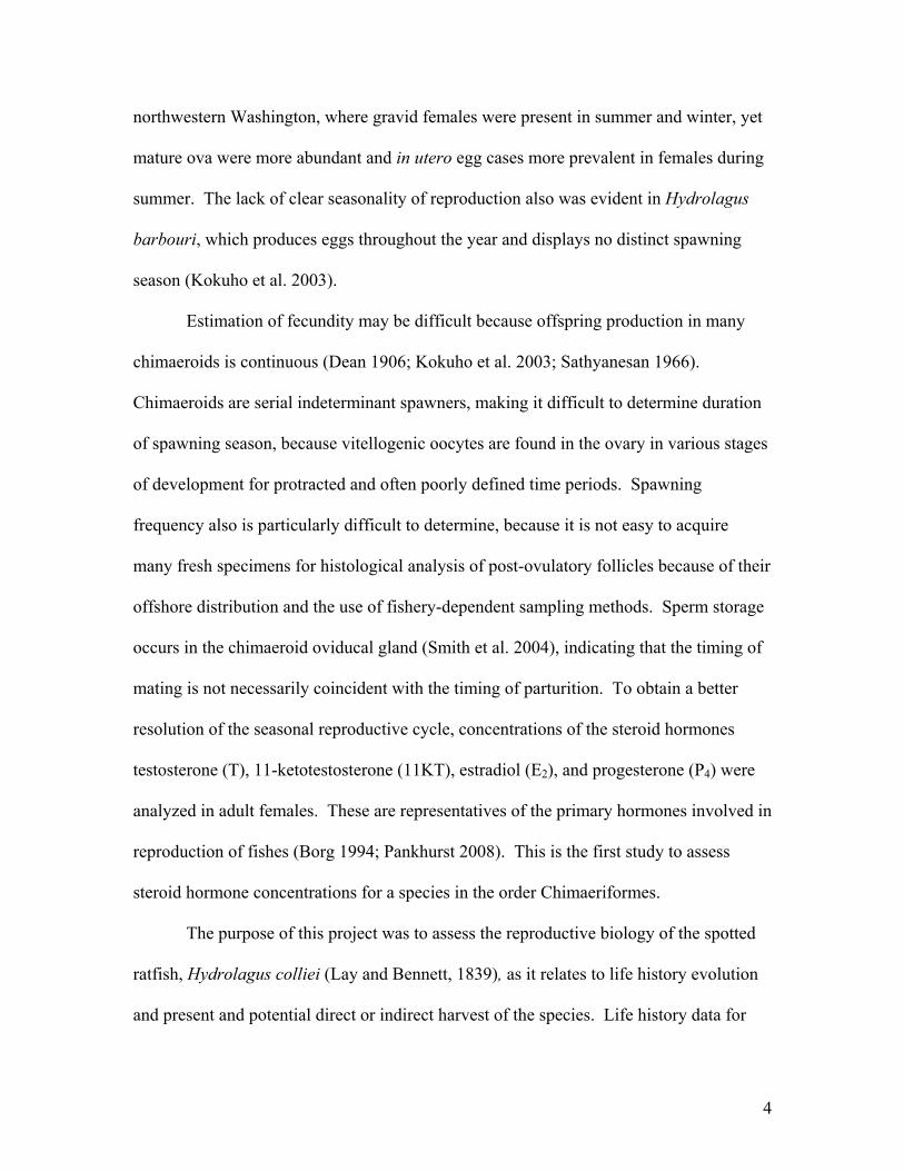
northwestern Washington, where gravid females were present in summer and winter, yet

mature ova were more abundant and in utero egg cases more prevalent in females during

summer. The lack of clear seasonality of reproduction also was evident in Hydrolagus

barbouri, which produces eggs throughout the year and displays no distinct spawning

season (Kokuho et al. 2003).

Estimation of fecundity may be difficult because offspring production in many

chimaeroids is continuous (Dean 1906; Kokuho et al. 2003; Sathyanesan 1966).

Chimaeroids are serial indeterminant spawners, making it difficult to determine duration

of spawning season, because vitellogenic oocytes are found in the ovary in various stages

of development for protracted and often poorly defined time periods. Spawning

frequency also is particularly difficult to determine, because it is not easy to acquire

many fresh specimens for histological analysis of post-ovulatory follicles because of their

offshore distribution and the use of fishery-dependent sampling methods. Sperm storage

occurs in the chimaeroid oviducal gland (Smith et al. 2004), indicating that the timing of

mating is not necessarily coincident with the timing of parturition. To obtain a better

resolution of the seasonal reproductive cycle, concentrations of the steroid hormones

testosterone (T), 11-ketotestosterone (11KT), estradiol (E2), and progesterone (P4) were

analyzed in adult females. These are representatives of the primary hormones involved in

reproduction of fishes (Borg 1994; Pankhurst 2008). This is the first study to assess

steroid hormone concentrations for a species in the order Chimaeriformes.

The purpose of this project was to assess the reproductive biology of the spotted

ratfish, Hydrolagus colliei (Lay and Bennett, 1839), as it relates to life history evolution

and present and potential direct or indirect harvest of the species. Life history data for

4

many eastern North Pacific chondrichthyans is lacking, yet it is necessary for proper

population assessment. This study provides estimates of the fecundity and seasonality of

parturition of H. colliei. These data provide a baseline of life history information for

chimaeroids, and are used to quantitatively test the hypotheses that fecundity is greater in

oviparous than viviparous chondrichthyan lineages and that length of reproductive season

increases with increasing depth range.

Materials and Methods

Specimens were collected from the continental slope and shelf of California,

Oregon, and Washington, with the greatest number of samples off Monterey Bay,

California (Fig. 1). Monterey Bay samples were collected from monthly trawl and long-

line surveys from October, 2003 to April, 2005 (conducted by NOAA NMFS, Southwest

Fisheries Science Center, Santa Cruz Laboratory). Trawls conducted by the Northwest

Fishery Science Center West Coast Groundfish Survey between May and October during

2004 to 2007 provided specimens from numerous locations off the coast of California,

Oregon, and Washington.

To define stage of reproductive development I measured various morphometrics.

Lengths were measured to the nearest mm and mass to the nearest gram. External

measurements of precaudal length (PCL), snout-vent length (SVL), and inner clasper

length were recorded following Didier and Rosenberger (2002). I measured total mass,

liver mass, gonad mass, seminal vesicle mass, testes length, testes width, oviducal gland

width, and uterus width. The number of mature ova (those greater than 6 mm diameter

with yellow coloration; Stanley 1961), fully developed ova (those greater than 20 mm

5

diameter; Stanley 1961), and diameter of the largest ovum were recorded from each

ovary.

Blood was extracted into lithium heparinized microcentrifuge tubes from a subset

of males and females via cardiac puncture shortly after capture. Blood samples were put

on ice for 1-3 h, then centrifuged at ~ 1,300 g for 10 min. Plasma was pipetted off into

microcentrifuge tubes and stored frozen at -18° C for later analysis. Skeletal muscle

tissue was excised from the dorsum, just posterior to the uterine openings.

Before hormone assay, plasma samples were thawed, centrifuged at 14,000 g for

5 min, and 500 µl of plasma was transferred to 12 x 75 mm borosilicate vials. Ether

extractions were conducted. Briefly, 2 ml diethyl ether was added to each borosilicate

vial, and the sample was vortexed for 4 min on a multi-tube vortexer. The ether and

aqueous phases were allowed to separate for 3 min, and the aqueous phase was then fast-

frozen in a methanol-dry ice bath for 2 min before decanting the ether phase into a new

12 x 75 mm borosilicate vial. The procedure was repeated on the remaining aqueous

phase, and the second ether sample was decanted into the same vial as the first. Ether

was evaporated under a gentle stream of nitrogen in a 37º C water bath. Extracts were

resuspended in 2 ml 0.1 M phosphate buffer for assay (1: 4 dilution).

Two muscle samples of ~ 500 mg were used for the T/11KT (mean ± SE: 517 ± 1

mg) and the E2/P4 assays (mean ± SE: 515 ± 2 mg). These muscle samples were excised

from a large piece of tissue on dry ice, weighed, transferred directly to 1 to 2 ml borate

buffer in a 12 x 75 mm borosilicate vial, and homogenized for 30 sec. Homogenate was

transferred to a 16 x 125 mm borosilicate vial and 4 ml diethyl ether was added to the

sample followed by vortexing for 4 min on a multi-tube vortexer. The ether and aqueous

6

phases were allowed to separate for 2 min, followed by centrifugation at 5,6000 g for 1

min at 4º C to pellet lipids in the tissue mass, and fast-freezing of the aqueous layer in a

methanol-dry ice bath for 2 min before decanting the ether phase. As with the plasma,

this procedure was repeated, ether layers were combined, and ether was evaporated.

Hormone pellets were stored at -20º C until reconstitution in 250 µl 0.1 M phosphate

buffer and assay. Reconstitution volume was determined from pilot assays, which I used

to evaluate the volume necessary to fall within the linear range of the T/11KT and E2/P4

standard curves.

Plasma and muscle samples from males were assayed for T and 11KT, and

samples from females were assayed for T, 11KT, E2, and P4. Samples were analyzed for

P4 and E2 using coated-tube and double antibody radioimmunoassay kits, respectively

(Siemens Medical Solutions Diagnostics, Los Angeles, CA). Samples were analyzed for

T with double antibody radioimmunoassay kits from Diagnostic Systems Laboratories

(Webster, TX), and for 11KT with enzyme-immunoassay kits (Cayman Chemicals, Ann

Arbor, MI). Manufacturer’s protocols were strictly followed. A control sample was

generated from 20, 500 mg muscle samples processed in the same manner as described

above, resuspended in 300 µl 0.1 M phosphate buffer, and pooled (6 ml). Aliquots (6, 1

ml samples) were used for intra- and inter-assay controls. Testosterone was quantified in

two separate assays with intra-assay coefficients of variation (CVs) of 2.86% and 3.56%,

and inter-assay CV of 4.21%. 11-Ketotestosterone was assayed on 7, 96-well plates with

intra-assay CVs of 9.22%, 20.4%, 12.9%, 11.9%, 15.5%, and 15.7%, and an inter-assay

CV of 16.7%. Estradiol was quantified in two separate assays with intra-assay CVs of

7

10.3% and 4.5%, and inter-assay CV of 8.3%. Progesterone was quantified in one assay

with an intra-assay CV of 9.9%.

Each kit was validated for H. colliei muscle steroids by generating serial dilutions

of the control sample (see previous paragraph) and assessing parallelism with the

standard curve using a t-test. Significant parallelism was achieved for all hormones

except progesterone (11KT: t = 0.025, df = 8, p = 0.98; T: t = 1.614, df = 6, p = 0.2; E2: t

= 1.95, df = 6, p = 0.1; P4: t = 7.08, df = 8, p < 0.001); the serial dilution curve for P4

exhibited a steep negative slope relative to the standard curve. Recovery was assessed by

spiking the control sample with each kit standard, and by determining the relationship

between expected (based on known control concentration) and observed concentrations.

Slopes of all observed vs. expected regressions approximated 1.0, indicating good

recovery (11KT: F = 80.63, df = 1, 7, p < 0.001, β1 = 1.05, minimum recovery = 69%; T:

F = 5928.7, df = 1, 6, p < 0.001, β1 = 1.26, minimum recovery = 96%; E2: F1,6 = 15.06, df

= 1, 6, p = 0.012, β1 = 0.75, minimum recovery = 111%; P4: F = 63.24, df = 1, 6, p =

0.0002, β1 = 0.71, minimum recovery = 58.4%). Sensitivities of the assays were 1.3

pg/ml for 11KT, 0.05 ng/ml for T, 1.4 pg/ml for E2, and 0.02 ng/ml for P4.

Weight-at-length data were analyzed with both sexes combined, because there

were no sex-specific trends. A non-linear regression was fit using the model that

produced the greatest adjusted R2 value, a two-parameter power function:

baLW =

Where W is weight in kg, L is snout-vent length in mm, a and b are estimated iteratively.

8

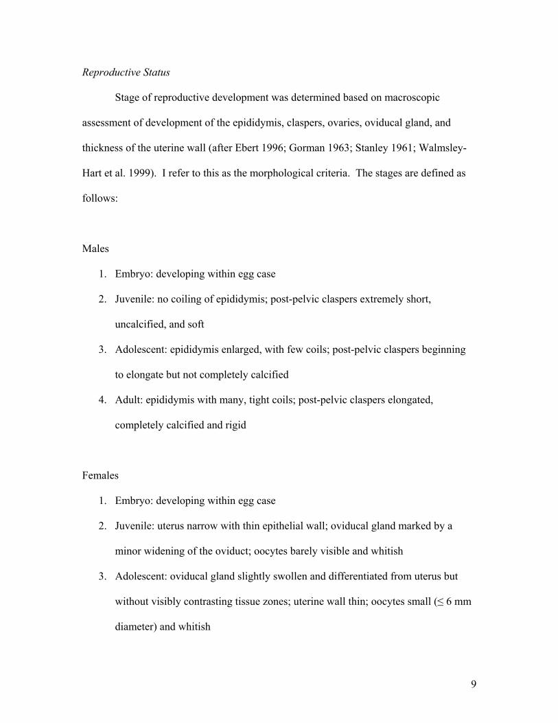
Reproductive Status

Stage of reproductive development was determined based on macroscopic

assessment of development of the epididymis, claspers, ovaries, oviducal gland, and

thickness of the uterine wall (after Ebert 1996; Gorman 1963; Stanley 1961; Walmsley-

Hart et al. 1999). I refer to this as the morphological criteria. The stages are defined as

follows:

Males

1. Embryo: developing within egg case

2. Juvenile: no coiling of epididymis; post-pelvic claspers extremely short,

uncalcified, and soft

3. Adolescent: epididymis enlarged, with few coils; post-pelvic claspers beginning

to elongate but not completely calcified

4. Adult: epididymis with many, tight coils; post-pelvic claspers elongated,

completely calcified and rigid

Females

1. Embryo: developing within egg case

2. Juvenile: uterus narrow with thin epithelial wall; oviducal gland marked by a

minor widening of the oviduct; oocytes barely visible and whitish

3. Adolescent: oviducal gland slightly swollen and differentiated from uterus but

without visibly contrasting tissue zones; uterine wall thin; oocytes small (≤ 6 mm

diameter) and whitish

9

4. Adult: oviducal gland fully developed with bulbous bullet-shape and sharply

contrasting tissue zones; uterine wall thick, especially proximal to uterine

openings where it is muscular and resistant to compression; oocytes large (> 6

mm diameter), yellow, and vascularized

5. Gravid Adult: fully or partially developed egg case present in uteri

During the assessment of maturity status of males using the morphological

criteria, a correspondence was observed between the stages of maturity defined above,

and distinct stages of frontal tenaculum development as defined below:

1. Juvenile: frontal tenaculum not yet erupted

2. Adolescent: frontal tenaculum erupted, yet not fully developed, with hooks

uncalcified or not present

3. Adult: frontal tenaculum fully developed with calcified hooks

This correspondence was tested by regressing maturity stages estimated using the

frontal tenaculum criteria on stages estimated using the morphological criteria, testing the

hypothesis that 11 =β (1:1 agreement of maturity stage) with a t-test.

To verify maturity status in males, the ratio of inner clasper length to body length

was plotted against body length. For females, the ratio of oviducal gland width to body

length was plotted against body length. An abrupt change in the proportion of these

ratios to body length was assumed to represent onset of maturity. Testis length was

plotted against inner clasper length, to test whether growth of internal and external

10

reproductive organs was collinear and whether abrupt increases in size, associated with

maturation, were concurrent.

Length at 50% maturity was estimated using a logistic regression equation

(Mollet et al. 2000; Neer and Cailliet 2001; Roa et al. 1999). To test for differences of

length at maturity between sexes and geographic regions, these factors were included as

main effects in a binomial logistic regression. Geographic regions were defined as north

or south of Point Conception or Cape Mendocino, two coastal promontories which create

oceanographic anomalies. Planned pairwise comparisons among regions were performed

with an experiment-wise error rate of α = 0.0125. To identify the temporal relationship

of steroid hormone production and onset of maturity, estimates of size at median maturity

derived from the morphological criteria were compared with estimates derived from the

concentration of T in the skeletal muscle of males and E2 from females. To create a

steroid hormone criterion, maturity status was assigned to individuals based on a

threshold concentration, assumed to indicate the onset of maturity. Threshold

concentrations were estimated by identifying an abrupt increase of steroid hormone

concentration with snout-vent length. Analysis of Residual Sums of Squares (ARSS) was

used to determine whether the logistic regression equations used to predict length at

maturity differed between morphological and hormone maturity criterion (Chen et al.

1992).

Reproductive Seasonality

Wet weights of the liver, gonads, and oviducal glands were measured to the

nearest gram, and expressed as a ratio of total mass as the hepatosomatic (HSI),

11

gonadosomatic (GSI), and oviducalsomatic indices (OGI), respectively. These indices,

calculated from a sample representative of all seasons, were plotted against month of

capture to determine whether temporal parturition patterns occurred, thus increasing

precision of fecundity estimates. Such indices alone, however, may not provide enough

evidence to estimate periodicity of parturition, as for batoids (Maruska et al. 1996).

Steroid hormone analysis, therefore, was used to verify reproductive seasonality in

females.

Temporal trends in steroid hormone concentrations of plasma and skeletal muscle

were compared with a series of t-tests. During two surveys off southern Oregon in early

June and early September, 2006, paired samples of plasma and skeletal muscle were

sampled from each individual. Temporal differences in levels of each hormone were

tested separately within plasma and muscle, to verify that trends were similar between the

two, as they are in the teleost fish Mycteroperca microlepis (Heppell and Sullivan 2000).

Among individuals from both sampling periods, correlation between plasma and muscle

hormone concentration was tested for each hormone separately.

A pilot test was used to determine whether the variable delay of sampling or

freezing of specimens subsequent to capture was a source of measurement error in the

greater study. For a subset of individuals, muscle tissue was sampled immediately after

capture, and again after specimens remained at ambient sea surface temperature for three

h. Paired t-tests were performed separately for each hormone to detect whether hormone

concentrations were affected by the difference in length of time between capture and

sampling or freezing of specimens.

12

Seasonal changes in OGI, the number of mature ova per female, and tissue

concentrations of steroid hormones were tested with ANOVA. Assumptions of normality

and were tested with Kolmogorov-Smirnoff tests, and homoscedacity with Levene’s tests.

Post-hoc multiple comparison tests were performed using Hotchberg’s GT2 test, because

sample sizes were greatly uneven. Kruskal-Wallis tests were used to compare seasonal

changes in the number of fully developed ova per female, HSI, and GSI, because of

heteroscedacity. For these non-parametric statistics, post-hoc multiple comparisons tests

were performed using the Nemenyi-Damico-Wolfe-Dunn test (Hollander and Wolfe

1999; Hothorn et al. 2006). Least-squares regression analyses were used to test the

hypothesis that length of spawning season of demersal chondrichthyan species increases

with increasing midpoint of bathymetric range (Table 1; data for chimaeroid species from

multiple ocean basins and elasmobranchs from the eastern North Pacific).

To estimate a maximum annual fecundity (the number of offspring produced per

year), the observed rate of parturition (egg cases deposited / week) from each of two

captive H. colliei at the Monterey Bay Aquarium was multiplied by the number of weeks

in a year. To estimate a realized annual fecundity, the maximum annual fecundity was

multiplied by the estimate of the proportion of the year the wild adult population is

spawning, as determined with steroid hormones, indices of organ weights, and presence

of in utero egg cases and mature ova in adult females. Descriptions of mating and egg-

laying of captive H. colliei were provided from personal observations of Gilbert Van

Dykhuizen, of the Monterey Bay Aquarium. Fecundity of chimaeroid species (n = 2) was

quantitatively compared with that of other chondrichthyans (Table 2) with a series of

randomization tests (α = 0.05). Mean fecundity was compared between viviparous

13

species and oviparous species with a t-test. Fecundity for each species was estimated as

the midpoint of the range reported in the literature, or the average if available. Before

testing, least-squares linear regression analyses were used to test for increasing fecundity

with increasing maximum size (TL, or DW when TL not available) among species within

each species group. Groups with significant effects of size on fecundity were split into

separate groups by a size threshold that minimized within-group variance in fecundity.

The randomization test solved the problem of heteroscedacity by comparing observed

mean differences among species groups to a null distribution of 100,000 mean

differences, each generated by bootstrapping two samples, each with two replicates, from

the pooled fecundities and calculating the difference between means. The latter analysis

was performed in the statistical computing environment R, version 2.4.1 (R Development

Core Team 2007). All comparisons among taxa were based on the classification system

of Compagno (1999).

Differences between oocyte size distribution of left and right ovaries of mature

females were tested with a Kolmogorov-Smirnov test. The number of mature oocytes,

and maximum ovum size per adult female were tested for potential increase with body

length, using least-squares regression.

Results

The relationship between body weight and length was described by the equation

(R2 = 0.939; Fig. 2). Snout-vent length was not measured

for all individuals. A linear regression of SVL on PCL, however, provided a good fit

(males: n = 237, SVL = 0.556(PCL) - 1.358, R2 = 0.987; females: n = 474, SVL =

( ) ( ) 755.2710459.2 SVLkgW −×=

14

0.576(PCL) - 4.097, R2 = 0.988), therefore, the resulting sex-specific linear equations

were used to predict the missing SVL values.

Maturity

An abrupt increase in the ratio of inner clasper length to snout-vent length with

increasing snout-vent length corresponded well with onset of maturity (n = 252; Fig. 3),

with few exceptions. The timing and scale of the abrupt increase in inner clasper length

were similar to those of testis length (t = 63.062, df = 213, p < 0.001, R2 = 0.949; Fig. 4).

Testis length was a suitable proxy for testicular growth, as testes grew isometrically in

length and width (t = 63.208, df = 222, R2 = 0.947, p < 0.001; Fig. 5). Male maturity

assessments using the frontal tenaculum development criterion were not significantly

different from assessments using the morphological criteria (t = 1.450, df = 213, R2 =

0.973, p = 0.2; Fig. 6). These results indicate that accurate estimates of maturity can be

deduced from male external morphology, and therefore do not necessarily require lethal

sampling techniques.

The purpose of the frontal tenaculum and prepelvic claspers was revealed during

two observations of mating at the Monterey Bay Aquarium (Gilbert Van Dykhuizen,

pers. comm.). Males used their frontal tenaculum to grapple the pectoral fin of the

female, and subsequently the prepelvic clasper was attached to the female’s ventrum,

corroborating previous observations (Didier and Rosenberger 2002). A single bifid

clasper was inserted into the female, with each terminal lobe swelling to 2 cm in diameter

after insertion into one of the two uterine openings. The mating pairs swam around the

tank in a normal swimming posture, side by side, while copulating for ~ 37 to 120 min.

15

During parturition, egg cases took 18 to 30 h to completely emerge from the uterine

openings, then remained attached to the uterus by a thin filament for 3 to 6 d before

deposition.

Abrupt increases in the ratio of oviducal gland width to snout-vent length with

increasing snout-vent length corresponded well with onset of maturity, as determined by

morphological criteria (n = 476; Fig. 7). Uterus width also increased with maturity, but is

not displayed. A large, gelatinous mass was found in the accessory genital gland (also

termed “receptaculum seminis” or “digitiform gland”) of 89% of adult females (n = 198)

and only 5% of sub-adult females (n = 91).

Length at maturity varied significantly between sexes (χ2 = 219.098, df = 1, p <

0.001) and regions (χ2 = 25.296, df = 2, p < 0.001). For individuals from the entire survey

area, size at 50% maturity (Fig. 8a) was 202.8 mm SVL for females (95% CI: 199.0 -

206.4, R2 = 0.995, n = 530) and 157.2 mm SVL for males (95% CI: 154.1 - 160.4, R2 =

0.996, n = 278). Post-hoc sex-specific comparisons indicated that female size at maturity

differed between the region south of Point Conception and the two regions to the north

(south vs. central: χ2 = 6.650, df = 1, p = 0.010; south vs. north: χ2 = 6.937, df = 1, p =

0.008), whereas male size at maturity differed between the region north of Cape

Mendocino and the two regions to the south (north vs. central: χ2 = 15.175, df = 1, p <

0.001; north vs. south: χ2 = 21.922, df = 1, p < 0.001). Separate logistic curves were fit

for each sex and region for which length at maturity varied. Size at 50% maturity was

greater for females captured north of Point Conception (202.5 mm SVL; 95% CI: 198.2 -

206.7) than south (189.8 mm SVL; 95%CI: 186.4 - 191.3; Fig. 8d). Size at 50% maturity

16

was greater for males captured north of Cape Mendocino (163.1 mm SVL; 95% CI: 157.8

- 168.2) than south (147.3 mm SVL; 95% CI: 145.4 - 148.8; Fig. 8e).

Length at maturity was significantly different between maturity criterion within

the subset of females assayed for estradiol (F = 5.518, df = 3, 24, p = 0.01), but did not

differ within the subset of males assayed for testosterone (F = 1.774, df = 3, 10, p = 0.2).

Female size at maturity indicated by estradiol concentration (185.3 mm SVL; 95% CI:

180.7, 189.9) was less than indicated by the morphological criteria (192.7 mm SVL; 95%

CI: 190.0, 195.5; Fig. 8b). There was a trend of smaller size at maturity estimated by

testosterone concentration (153.5 mm SVL; 95% CI: 147.9, 159.3) than the

morphological criteria (159.7 mm SVL; 95% CI: 155.0, 164.3; Fig. 8c).

Smallest mature specimens were 190 mm SVL for females and 149 mm SVL for

males. Maximum and minimum sizes for each sex were north of Cape Mendocino.

Minimum size (male: 46 mm SVL; female: 41 mm SVL) is believed to be near size at

birth. Maximum size for males was 208 mm SVL (496 mm TL) and 283 mm SVL (633

mm TL) for females. Maximum size previously was reported as 965 mm TL (Miller and

Lea 1972), indicating this population has decreased dramatically in body size, that

original records were overestimated, or simply that the record represents an anomalous

individual.

Effects of differing sample collection methods

Temporal trends were similar between plasma and muscle for all hormones except

P4 (Fig. 9); however, none of the trends were significant (Table 1). There was a

significant positive correlation of hormone concentration between plasma and muscle

17

samples for T (χ2 = 9.626, r = 0.65, p = 0.002), 11KT (χ2 = 6.673, r = 0.563, p = 0.01),

and P4 (χ2 = 5.028, r = 0.457, p = 0.025), but not for E2 (χ2 = 1.516, r = 0.261, p = 0.2).

Concentrations were greater in plasma than muscle. Hormone concentrations of muscle

samples taken immediately after capture were not significantly different from samples

taken three hours later from the same individuals (Table 2); however, there was a slight

trend of decreasing concentration with time of sampling for E2 and P4 (Fig. 10).


Gravid females were detected in January, and May through October (Fig. 11).

The size-frequency distribution of oocytes did not differ between left and right ovaries

(Kolmogorov-Smirnov: Z = 0.955, p = 0.3), therefore, total number of ova per female

was used for analyses. The number of mature ova per female varied among months

(ANOVA: F = 4.543, df = 7, 167, p < 0.001; Fig. 12); significantly greater in late summer

and early fall than all other time periods (Hochberg GT2: df = 167, p ≤ 0.034). The

number of fully developed ova, 20 mm diameter or greater (Stanley 1961), varied

dramatically among months (Kruskal-Wallis: χ2 = 20.322, df = 10, p = 0.026; Fig. 13).

The seasonal presence of fully developed ova and in utero egg cases indicated 6-8 mo of

parturition per year.

Concentration of 11KT in muscle of females varied among months (ANOVA: F =

6.404, df = 6, 110, p < 0.001; Fig. 14); significantly greater in April than any other month

(Hochberg GT2: df = 110, p ≤ 0.001). Concentration of P4 in muscle of females varied

among months (ANOVA: F = 2.991, df = 10, 114, p = 0.002; Fig. 15); significantly

greater in January than June and September (Hochberg GT2: df = 114, p ≤ 0.003).

18

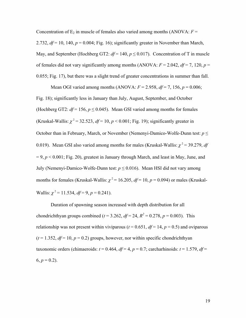
Concentration of E2 in muscle of females also varied among months (ANOVA: F =

2.732, df = 10, 140, p = 0.004; Fig. 16); significantly greater in November than March,

May, and September (Hochberg GT2: df = 140, p ≤ 0.017). Concentration of T in muscle

of females did not vary significantly among months (ANOVA: F = 2.042, df = 7, 120, p =

0.055; Fig. 17), but there was a slight trend of greater concentrations in summer than fall.

Mean OGI varied among months (ANOVA: F = 2.958, df = 7, 156, p = 0.006;

Fig. 18); significantly less in January than July, August, September, and October

(Hochberg GT2: df = 156, p ≤ 0.045). Mean GSI varied among months for females

(Kruskal-Wallis: = 32.523, df = 10, p < 0.001; Fig. 19); significantly greater in

October than in February, March, or November (Nemenyi-Damico-Wolfe-Dunn test: p ≤

0.019). Mean GSI also varied among months for males (Kruskal-Wallis: = 39.279, df

= 9, p < 0.001; Fig. 20), greatest in January through March, and least in May, June, and

July (Nemenyi-Damico-Wolfe-Dunn test: p ≤ 0.016). Mean HSI did not vary among

months for females (Kruskal-Wallis: = 16.205, df = 10, p = 0.094) or males (Kruskal-

Wallis: = 11.534, df = 9, p = 0.241).

2χ

2χ

2χ

2χ

Duration of spawning season increased with depth distribution for all

chondrichthyan groups combined (t = 3.262, df = 24, R2 = 0.278, p = 0.003). This

relationship was not present within viviparous (t = 0.651, df = 14, p = 0.5) and oviparous

(t = 1.352, df = 10, p = 0.2) groups, however, nor within specific chondrichthyan

taxonomic orders (chimaeroids: t = 0.464, df = 4, p = 0.7; carcharhinoids: t = 1.579, df =

6, p = 0.2).

19

Fecundity

Two captive H. colliei, taken from Puget Sound, WA, deposited 18 and 20 egg

cases, respectively, while monitored for 24 consecutive weeks from December 1996 to

June 1997 at the Monterey Bay Aquarium (Gilbert Van Dykhuizen, pers. comm.).

Annual fecundity was 19.5 to 28.9. The number of fully developed ova, 20 mm diameter

or greater (Stanley 1961), increased with adult female somatic weight (r = 0.394, df = 54,

p = 0.003; Fig. 21). Additionally, for reproductively active females, the maximum ovum

diameter increased with snout-vent length (t = 3.833, df = 159, R2 = 0.079, p < 0.001).

For the latter analysis, females were considered reproductively active if their ovaries

contained at least one follicle of 16 mm diameter or greater, a threshold that became

apparent when maximum ovum size was compared with snout-vent length (ANCOVA:

interaction term = maximum ovum size*snout-vent length; F = 7.734, df = 1, 203, p =

0.006; Fig. 22).

Fecundities differed between oviparous and viviparous species (t = 10.433, df =

83, p < 0.001); mean fecundity of viviparous species was less (8.1; SE = 0.94) than mean

fecundity of oviparous species (50.1; SE = 6.2). Fecundity decreased with size within the

order Squaliformes (t = 2.312, df = 12, p = 0.039), and therefore was separated into large

(TL > 60 cm) and small (TL < 60 cm) categories. There was no significant relationship

between fecundity and body size of other taxonomic orders. When these same species

were grouped by higher taxonomic level, the oviparous chimaeriform fishes had greater

fecundity than the viviparous lamniform (marginally significant; p = 0.052),

myliobatiform (p = 0.008), rhinobatiform (p = 0.021), and squaliform fishes (small: p =

20

0.044; large: p = 0.021), and similar fecundity to the oviparous rajiforms (p = 0.15) and

the carcharhiniforms (p > 0.9), with both reproductive modes represented.

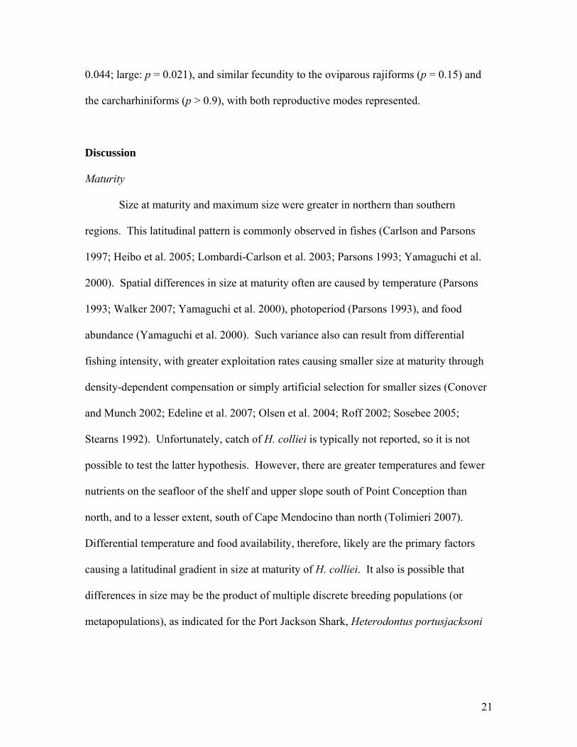
Discussion

Maturity

Size at maturity and maximum size were greater in northern than southern

regions. This latitudinal pattern is commonly observed in fishes (Carlson and Parsons

1997; Heibo et al. 2005; Lombardi-Carlson et al. 2003; Parsons 1993; Yamaguchi et al.

2000). Spatial differences in size at maturity often are caused by temperature (Parsons

1993; Walker 2007; Yamaguchi et al. 2000), photoperiod (Parsons 1993), and food

abundance (Yamaguchi et al. 2000). Such variance also can result from differential

fishing intensity, with greater exploitation rates causing smaller size at maturity through

density-dependent compensation or simply artificial selection for smaller sizes (Conover

and Munch 2002; Edeline et al. 2007; Olsen et al. 2004; Roff 2002; Sosebee 2005;

Stearns 1992). Unfortunately, catch of H. colliei is typically not reported, so it is not

possible to test the latter hypothesis. However, there are greater temperatures and fewer

nutrients on the seafloor of the shelf and upper slope south of Point Conception than

north, and to a lesser extent, south of Cape Mendocino than north (Tolimieri 2007).

Differential temperature and food availability, therefore, likely are the primary factors

causing a latitudinal gradient in size at maturity of H. colliei. It also is possible that

differences in size may be the product of multiple discrete breeding populations (or

metapopulations), as indicated for the Port Jackson Shark, Heterodontus portusjacksoni

21

(Tovar-Avila et al. 2007). There is insufficient evidence, however, to evaluate the latter

hypothesis.

Recent studies have indicated that assays of the steroid hormones T and E2 in

plasma serves as an accurate, non-lethal method of determining size at maturity for

chondrichthyans (Sulikowski et al. 2004). In this study, however, steroid hormone

maturity criteria predicted significantly smaller size at maturity than morphological

criteria for females, and a similar, yet insignificant trend for males. The differences were

not great in magnitude, but the results indicated that accuracy of maturity estimates from

hormone data was not perfect, and perhaps biased toward identification of smaller size at

maturity. In the teleost fish Mycteroperca microlepis neither E2 nor T from plasma or

muscle were consistent indicators of maturity (Heppell and Sullivan 2000).

It is logical that hormones related to maturity should increase before

morphological maturity, as T is correlated with development of intromittent organs

(Schreibman et al. 1986), and 11KT is correlated with expression of secondary sexual

physiological characters (Borg 1987; Borg et al. 1993; de Ruiter and Mein 1982; Hishida

and Kawamoto 1970; Idler et al. 1961; Pottinger and Pickering 1985). The synchronous

development of the frontal tenaculum and internal reproductive organs also was

observed, albeit qualitatively, in the elephant fish Callorhynchus milii (Gorman 1963).

Gorman (1963), however, also reported that prepelvic claspers were only present in adult

males, but they were omnipresent in H. colliei males. The gelatinous mass of the

accessory genital gland, which contains desquamated epithelial cells (Stanley 1963), was

found in 89% of mature females. The function of this secretion is unknown, but also was

present in nearly all mature females in a previous study (Stanley 1963).

22

The in situ observations of mating behavior recorded from captive H. colliei

resolved questions regarding the copulation and parturition process. It was previously

hypothesized that the frontal tenaculum was used for grappling the base of the female’s

dorsal fin during copulation (Dean 1903). The duration of the parturition process,

combined with observed captive parturition rates, is consistent with Dean’s (1903) 3 to 5

d estimate of duration of egg-case formation based on the progression of fertilization.

Stylasterias spp., Neptunia spp., and Icelinus filamentosus were observed on egg

cases in aquaria, perhaps attempting to predate upon them. In natural systems,

elasmobranch egg cases are preyed upon primarily by gastropods (Cox and Koob 1993;

Lucifora and Garcia 2004), but are occasionally eaten by fishes and other marine

vertebrates (Bor and Santos 2003). Predation rates of egg-cases by gastropods are 2 to

45% for skates (Hoff 2007), and 14 to 40% for a mixed group of skates and sharks off

South Africa (Smith and Griffiths 1997).


Fluctuations of T, 11KT, E2, and P4 are related to many important reproductive

events in oviparous fishes. 11-Ketotestosterone is correlated with pre-vitellogenic oocyte

growth (Matsubara et al. 2003), oocyte maturation (Semenkova et al. 2006), and

ovulation (Semenkova et al. 2006) in females, and sexual behavior in males (Borg 1987;

Kindler et al. 1991). Greater concentration in April is consistent with the apparent

function of 11KT in pre-parturition stages of reproduction. If the correlation with sexual

behavior is consistent for females, the observed peak also may be related to mating

activity. Although there was no clear physical evidence of mating activity, Dean (1903)

23

indicated that mating takes place shortly before parturition, based on the presence of fresh

mating scars on gravid females.

Testosterone is correlated with ovary recrudescence (Sumpter and Dodd 1979),

oocyte maturation (Semenkova et al. 2006), oviposition (Sumpter and Dodd 1979), and

encapsulation (Rasmussen et al. 1999), greatest just before increases in progesterone

associated with oviposition and egg capsule formation (Koob et al. 1986). Testosterone

is synthesized by developing follicles and luteal tissue, whereas estradiol is primarily

synthesized by developing follicles (Callard et al. 1993). The observed seasonal

fluctuation of T was not very distinct, but the increase during May through August may

be consistent with its role in oviposition and encapsulation.

Estradiol is correlated with ovarian recrudescence (Sulikowski et al. 2004;

Sumpter and Dodd 1979), increased oviducal gland weight (Sulikowski et al. 2004),

follicle size (Sulikowski et al. 2004), elevated plasma vitellogenin (Craik 1978; 1979; Ho

et al. 1980; Takemura and Kim 2001; Woodhead 1969), oviposition (Sumpter and Dodd

1979), and induction and maintenance of structural proteins and enzymes in the oviducal

glands (Dodd and Goddard 1961; Koob et al. 1986). Relative levels of E2 to P4 influence

oviduct contraction, with P4 acting as an inhibitor (Abrams-Motz and Callard 1989).

Estradiol may enhance sensitivity to relaxin, which may facilitate oviposition, gestation,

and parturition by allowing increased dilation of the reproductive tract (Koob et al. 1984)

and perhaps controlling smooth muscle action required for these processes (Callard et al.

1993). Conversely, P4 seems to inhibit the function of relaxin (Sorbera and Callard

1989). In H. colliei, E2 was greatest in November, and least from March through

24

October, indicating that its primary role may be preovulatory, particularly ovarian

recrudescence.

In oviparous chondrichthyans, P4 may increase extensibility and vascularization

of the uterine wall (Koob and Callard 1999) immediately before ovulation and

encapsulation (Koob and Hamlett 1998). Progesterone and its receptors may restrict rates

of folliculogenesis through a variety of pathways (Callard et al. 1995), including

inhibition of E2-induced vitellogenin gene transcription in the liver (Perez and Callard

1993). Progesterone is correlated with parturition (Sulikowski et al. 2004) and final

oocyte maturation (Semenkova et al. 2006). Progesterone is primarily synthesized by

luteal tissue (Callard et al. 1993; Fileti and Callard 1988). In this study, P4 was greatest

in January, and decreased through fall. This pattern is incongruous with the other

indicators of reproductive activity and the typical physiological effects of P4 on oviparous

chondrichthyans. The peak may be related to mating, however, as Heupel et al. (1999)

observed a peak in P4 just before the mating season in the viviparous shark Hemiscyllium

ocellatum.

Steroid hormone cycles of oviparous chondrichthyans have been generalized as a

synchronous cycle wherein E2 and P4 increase during follicular growth (preovulation) and

decrease during luteal development (Callard et al. 1991), with greatest levels of E2

slightly preceding those of P4 (Koob et al. 1986). This pattern was evident for H. colliei;

however, these maxima preceded maximum ovulatory activity by as long as 5 mo, a

greater duration than anticipated, especially considering the role of P4 in encapsulation

(Koob et al. 1986) and increased extensibility of the reproductive tract to accommodate

25

egg cases (Koob and Hamlett 1998). This discrepancy may represent the difference

between population and individual hormone cycles.

I found H. colliei had a discrete reproductive cycle, contradicting previous studies

(Dean 1906; Sathyanesan 1966). Duration and timing of the parturition season of H.

colliei was similar to that of Chimaera phantasma (Malagrino et al. 1981) and Chimaera

monstrosa (Vu-Tan-Tue 1972). It also was similar to callorhynchids (Bell 2003; Di

Giacomo and Perier 1994; Freer and Griffiths 1993b; Gorman 1963; review in

McClatchie and Lester 1994), which make inshore migrations for egg deposition and

have a shallower bathymetric range than chimaerids.

Discrete spawning periods are temporally regulated by social cues (Whittier and

Crews 1987), and environmental cues such as temperature (Danilowicz 1995; Goulet

1995; Hilder and Pankhurst 2003; Whittier and Crews 1987), photoperiod (Jobling 1995;

Whittier and Crews 1987), lunar phase (Robertson et al. 1990; review in Robertson

1991), illumination (Whittier and Crews 1987), and food abundance (Tyler and Stanton

1995; Whittier and Crews 1987). In temperate zones, the most common cue is

photoperiod, with some influence of temperature (Jobling 1995; Whittier and Crews

1987). Length of reproductive season is greater in tropical than temperate zones (Jobling

1995). Duration of reproductive season also may be correlated with the amount of

primary productivity (Whittier and Crews 1987).

The current paradigm regarding reproductive seasonality in the marine

environment is that animals that inhabit deeper depths are less likely to have seasonal

cycles of reproductive output (Parsons and Grier 1992; Wourms 1977). Although this

relationship was present when analyzing all chondrichthyans combined, it was not

26

apparent when oviparous and viviparous species were analyzed separately, indicating an

artefact of reproductive mode. The effect also was not significant within the chimaeroids

or carcharhinoids. It is not surprising that this generalization is faulty. Recent

researchers have shown that productivity from coastal upwelling can have a major

influence on benthic communities as deep as 4,100 m (Ruhl and Smith 2004). These new

insights indicate that the evolution of discrete versus continuous reproductive cycles is a

much more complex process than previously thought.

Hydrolagus colliei has a constant or endogenous reproductive cycle (Whittier and

Crews 1987). In the former situation, the gonads are always prepared for reproduction,

but sexual behavior is cued by environmental conditions, and in the latter situation,

reproductive activity is seasonal, but has minimal environmental regulation. Under these

criteria, H. colliei has constant cycle, because parturition of the wild population coincides

with dramatic annual environmental changes in thermocline depth and primary

productivity. Captive H. colliei at the Monterey Bay Aquarium have extruded egg cases

during all seasons, which also may be evidence for the environmental regulation of

reproductive activity. Alternatively, reproductive activity could be regulated by social

cues, with captive individuals remaining constantly reproductively active due to the

perpetual proximity of males, a situation that is not probable in some wild

chondrichthyan populations (Economakis and Lobel 1998). Further evidence for an

endogenous cycle regulated by social cues is provided by Bell (2003), in which captive

female Callorhinchus milii, in the absence of males, retained their annual reproductive

cycle while temperature and photoperiod were kept relatively stable.

27

Fecundity

The simple method of fecundity estimation by extrapolation of observed

parturition rates was used instead of methods of Holden (1975) because assumptions of

Holden’s methods likely were violated. Holden (1975) used the proportion of gravid

individuals sampled from the wild population as a proxy for the proportion of the

population depositing egg-cases during a given period of time. A primary assumption of

this method is that the gravid population is being appropriately sampled. This

assumption is likely not met for H. colliei, as parturition in this species occurs primarily

on or around seamounts. These regions are poorly represented in surveys because they

comprise an exceptionally small area of the seafloor and their rocky, rugose surface

cannot be sampled with trawl gear. Holden’s (1975) alternative method of estimating

fecundity relies upon the following assumptions: (1) all mature ova produced by an adult

female during a given year are formed before the onset of parturition, and therefore are

simultaneously present in the ovary; (2) this group of mature ova will all be placed in egg

cases and extruded during the current spawning season; and (3) no ovum resorption

occurs. It is doubtful that these assumptions are met for H. colliei, in which ovum

resorption and/or follicle atresia were commonly observed. The number of mature and

fully developed ova in females and female GSI do not decrease gradually toward the end

of the spawning season (Figs. 12, 13, 19), as would be expected if the former two

assumptions were met.

Fecundity of H. colliei is similar to that estimated for Callorhinchus milii (16-24;

Bell 2003), but much greater than that estimated for Chimaera monstrosa (mean = 6;

Moura et al. 2004). The latter discrepancy, however, could be caused in part by the

28

method of fecundity estimation. Moura et al. (2004) estimated fecundity by calculating

the mean number of fully developed ova per adult female. Similarly, Tovar-Avila et al.

(2007) estimated fecundity for Heterodontus portjacksoni, a shark with single oviparous

reproductive mode, as the mean number of oocytes ≥ 75% of ovulatory size in adult

female sharks in the months before the parturition season. The latter method provided

similar estimates to that derived by extrapolation of captive parturition rates (Tovar-Avila

2006). In H. colliei, however, the mean number of oocytes greater than 10 mm diameter

(≥ ~ 35-50% of ovulatory size) per female captured before the egg-laying season was

only 10 (range = 1-36; σ = 9.04; n = 32), less than half the mean fecundity estimated from

captive parturition rates. This discrepancy indicates that the method of simply

enumerating maturing ova may be inadequate for chimaeroids, and other chondrichthyans

with single oviparity that display rapid vitellogenesis (e.g. Holden et al. 1971) and

protracted production of mature ova.

Fecundity estimation for chondrichthyans with single oviparity is a difficult and

uncertain process, with extrapolation of captive parturition rates often providing the most

accurate fecundity estimates. In my study, fecundity of H. colliei was 19.5-28.9, but it

may be much less, as some of the egg cases deposited in captivity were ruptured or not

completely formed during parturition. Additionally, only 10% of egg cases deposited in

captivity were fertile (n = 38). The phenomenon of “gel eggs,” or egg cases without an

ovum and containing only egg jelly, may be another factor reducing fecundity in natural

populations. Although gel eggs have not been observed in chimaeroids, Hoff (2007)

reported that gel eggs composed nearly 5% of all in utero egg cases in Bering Sea skates.

29

Incorporation of embryonic survival, therefore, will greatly improve fecundity estimates

derived from extrapolation of captive parturition rates.

The number of fully developed ova increased with adult female somatic weight,

providing marginally significant evidence for increased fecundity with size. This effect

occurs in another chimaeroid, Callorhinchus milii (Bell 2003), and other organisms,

including skates (Matta 2006), sharks (Simpfendorfer 1992; Yano 1995), and rockfishes

(Bobko and Berkeley 2004; Boehlert et al. 1982; Cooper et al. 2005). There also is some

evidence for increasing maximum ovum size with maternal body size. Larger females

may provide more nutrients to their young, potentially increasing offspring fitness

(Berkeley et al. 2004a). Increased embryo, egg, egg case, or yolk sac size and/or nutrient

content with larger maternal size occurs in many fishes, including skates (Hoff 2007),

sharks, and rockfish (Berkeley et al. 2004a). Increased number and fitness of offspring

with increased maternal size is an important biological component in conservation

planning (Berkeley et al. 2004b). Although there are many chondrichthyans with one of

the two maternal size effects observed in H. colliei, there are few species that exhibit both

(Cortes 2000). There seems to be a tradeoff between the number of offspring and

offspring size within and among chondrichthyan populations (review in Cortes 2000),

indicating the existence of a specific ratio of the two that would maximize fitness (Roff

2002).

Previously oviparity was considered the plesiomorphic state of chondrichthyans

(Compagno 1990; Dulvy and Reynolds 1997; Wourms 1977; Wourms and Lombardi

1992), but a recent review indicated that viviparity is the ancestral state (Musick and Ellis

2005). Musick and Ellis (2005) revisited the ideas of Holden (1973) and hypothesized

30

that oviparity evolved to increase fecundity in small-bodied species, which have too little

coelomic space to produce many live offspring per litter. Support for this hypothesis is

provided by the trend for fecundity in oviparous than viviparous species of small body

size, a phenomena that was previously disputed (Wourms and Lombardi 1992). In this

study, fecundity was quantitatively compared among chondrichthyan lineages to provide

more explanatory power for these hypotheses by incorporating interpretation of fecundity

evolution into the evolution of reproductive modes.

A current paradigm indicates that viviparous species of chondrichthyans are less

fecund than their oviparous counterparts. To quantitatively test this theory, I compared

fecundities for oviparous and viviparous species from the orders Carcharinhiformes (n =

20), Rajiformes (n = 12), Rhinobatiformes (n = 9), Myliobatiformes (n = 19),

Torpediniformes (n = 2), Chimaeriformes (n = 2), Squaliformes (n = 14), Lamniformes (n

= 4), Rhiniformes (n = 1) and Orectolobiformes (n = 2). It should be noted that the two

rajiforms with multiple oviparity, Raja binoculata and Raja pulchra, were considered

outliers because of their potential to produce many more offspring than other rajiforms

(Ebert and Davis 2007), and therefore were excluded from analyses. Mean fecundity of

viviparous species was less than mean fecundity of oviparous species. When those same

species were grouped by higher taxonomic level, the oviparous chimaeriform fishes had

greater fecundity than the viviparous lamniform, squaliform, and rhinobatiform fishes,

but similar fecundity to the oviparous rajiforms and the mixed carcharhiniforms. There

was a trend of greater mean fecundity for Rajiformes (56.4) than Chimaeriformes (22.1).

These results indicate that the oviparous Chimaeriformes evolved greater fecundity than

their viviparous elasmobranch relatives, but perhaps lesser fecundity than the more

31

derived oviparous species within the order Rajiformes. With the Chimaeriformes added

into the analysis of evolution of fecundity, more evidence is provided that supports the

hypothesis of viviparous plesiomorphy in chondrichthyans, as argued by Musick and

Ellis (2005).

32

Literature Cited

Abrams-Motz V, Callard IP (1989) Seasonal variations in oviduct myometrial activity,

extensibility and tensile strength in Chrysemys picta. General and Comparative

Endocrinology 72: 453-460

Alverson DL, Pruter AT, Ronholt LL (1964) A study of demersal fishes and fisheries of

the northeastern Pacific Ocean. H.R. MacMillan Lectures in Fisheries. Institute

of Fisheries, University of British Columbia, Vancouver

Anon (1997) Report of the study group of elasmobranch fishes. ICES CM 1997/G:2

Barnett LAK, Dagit DD, Long DJ, Ebert DA (2006) Hydrolagus mccoskeri sp. nov., a

new species of chimaeroid fish from the Galápagos Islands (Holocephali:

Chimaeriformes: Chimaeridae). Zootaxa 1328: 27-38

Bell JD (2003) Fisheries and reproductive biology of the elephant fish, Callorhinchus

milii, in south-east Australia. Bachelor of Environmental Science (honours).

Deakin University

Berkeley SA, Chapman C, Sogard SM (2004a) Maternal age as a determinant of larval

growth and survival in a marine fish, Sebastes melanops. Ecology 85: 1258-1264

Berkeley SA, Hixon MA, Larson RJ, Love MS (2004b) Fisheries sustainability via

protection of age structure and spatial distribution of fish populations. Fisheries

29: 23-32

Bobko SJ, Berkeley SA (2004) Maturity, ovarian cycle, fecundity, and age-specific

parturition of black rockfish (Sebastes melanops). Fishery Bulletin 102: 418-429

Boehlert GW, Barss WH, Lamberson PB (1982) Fecundity of the widow rockfish,

Sebastes entomelas, off the coast of Oregon. Fishery Bulletin 80: 881-884

33

Bonfil R (1994) Overview of world elasmobranch fisheries. FAO Technical Paper 341

Bor PHF, Santos MB (2003) Findings of elasmobranch eggs in the stomachs of sperm

whales and other marine organisms. Journal of the Marine Biological Association

of the U.K. 83: 1351-1353

Borg B (1987) Stimulation of reproductive behaviour by aromatizable and non-

aromatizable androgens in the male three-spined stickleback, Gasterosteus

aculeatus L. In: Kullander SOK, Fernholm B (eds) Proc. 5th Congr. Eur. Ichthyol.

Stockholm. Swedish Museum of Natural History, Stockholm, pp 269-271

Borg B (1994) Androgens in teleost fishes. Comparative Biochemistry and Physiology

Part C: Comparative Pharmacology and Toxicology 109: 219-245

Borg B, Antonopoulou E, Andersson E, Carlberg T, Mayer I (1993) Effectiveness of

several androgens in stimulating kidney hypertrophy, a secondary sexual

character, in castrated male three-spined stickleback, Gasterosteus aculeatus.

Canadian Journal of Zoology 71: 2327-2329

Cailliet GM (1990) Elasmobranch age determination and verification: an updated review.

In: Pratt Jr HL, Gruber SH, Taniuchi T (eds) Elasmobranchs as living resources:

advances in the biology, ecology, systematics, and the status of the fisheries.

NOAA Technical Report 90, pp 157-165

Cailliet GM, Andrews AH, Burton EJ, Watters DL, Kline DE, Ferry-Graham LA (2001)

Age determination and validation studies of marine fishes: do deep-dwellers live

longer? Experimental Gerontology 36: 739-764

34

Cailliet GM, Goldman KJ (2004) Age determination and validation in chondrichthyan

fishes. In: Carrier JC, Musick JA, Heithaus MR (eds) Biology of sharks and their

relatives. CRC Press, Boca Raton, FL, pp 399-448

Callard IP, Etheridge K, Giannoukos G, Lamb T, Perez L (1991) The role of steroids in

reproduction in female elasmobranchs and reptiles. Journal of Steroid

Biochemistry and Molecular Biology 40: 571-575

Callard IP, Fileti LA, Koob TJ (1993) Ovarian steroid synthesis and the hormonal control

of the elasmobranch reproductive tract. Environmental Biology of Fishes 38: 175-

185

Callard IP, Putz O, Paolucci M, Koob TJ (1995) Elasmobranch reproductive life-

histories: endocrine correlates and evolution. Proceedings of the International

Symposium on the Reproductive Physiology of Fish, Austin, TX, pp 204-208

Carlson JK, Parsons GR (1997) Age and growth of the bonnethead shark, Sphyrna tiburo,

from northwest Florida, with comments on clinal variation. Environmental

Biology of Fishes 50: 331-341

Chen Y, Jackson DA, Harvey HH (1992) A comparison of von Bertalanffy and

polynomial functions in modelling fish growth data. Canadian Journal of

Fisheries and Aquatic Sciences 49: 1228-1235

Clarke MW, Kelly CJ, Connolly PL, Molloy JP (2003) A life history approach to the

assessment and management of deepwater fisheries in the northeast Atlantic.

Journal of Northwest Atlantic Fishery Science 31: 401-411

Compagno LJV (1990) Alternative life-history styles of cartilaginous fishes in time and

space. Environmental Biology of Fishes 28: 33-75

35

Compagno LJV (1999) Checklist of living elasmobranchs. In: Hamlett WC (ed) Sharks,

skates, and rays: the biology of elasmobranch fishes. The Johns Hopkins

University Press, Baltimore, Maryland

Compagno LJV (2005) Checklist of living Chondrichthyes. In: Hamlett WC (ed)

Reproductive biology and phylogeny of Chondrichthyes: sharks batoids and

chimaeras. Science Publishers, Inc., Enfield, pp 503-548

Conover DO, Munch SB (2002) Sustaining fisheries yields over evolutionary time scales.

Science 297: 94-96

Cooper DW, Pearson KE, Gunderson DR (2005) Fecundity of shortspine thornyhead

(Sebastolobus alascanus) and longspine thornyhead (S. altivelis) (Scorpaenidae)

from the northeastern Pacific Ocean, determined by stereological and gravimetric

techniques. Fishery Bulletin 103: 15-22

Cortes E (2000) Life history patterns and correlations in sharks. Reviews in Fisheries

Science 8: 299-344

Cox DL, Koob TJ (1993) Predation on elasmobranch eggs. Environmental Biology of

Fishes 38: 117-125

Craik JCA (1978) An annual cycle of vitellogenesis in the elasmobranch Scyliorhinus

canicula L. Journal of the Marine Biological Association of the United Kingdom

58: 719-726

Craik JCA (1979) Simultaneous measurement of rates of vitellogenin synthesis and

plasma levels of estradiol in an elasmobranch. General and Comparative


36

Cross JN (1981) Structure of a rocky intertidal fish assemblage. Ph.D. Thesis, University

of Washington

Danilowicz BS (1995) Spatial patterns of spawning in the coral-reef damselfish

Dascyllus albisella. Marine Biology 122: 145-155

de Ruiter AJH, Mein CG (1982) Testosterone-dependent changes in vivo and in vitro.

General and Comparative Endocrinology 47: 70-83

Dean B (1903) An outline of the development of a chimaeroid. Biological Bulletin 4:

270-286

Dean B (1906) Chimaeroid fishes and their development. Carnegie Institute Publication,

Washington, D.C.

Di Giacomo EE, Perier MR (1994) Reproductive biology of the cockfish, Callorhynchus

callorhinchus (Holocephali: Callorhynchidae), in Patagonian waters (Argentina).

Fishery Bulletin 92: 531-539

Didier DA (1995) Phylogenetic systematics of extant Chimaeroid fishes (Holocephali,

Chimaeroidei). American Museum Novitates 3119: 1-86

Didier DA, LeClair EE, Vanbuskirk DR (1998) Embryonic staging and external features

of development of the chimaeroid fish, Callorhinchus milii (Holocephali,

Callorhinchidae). Journal of Morphology 236: 25-47

Didier DA, Rosenberger LJ (2002) The spotted ratfish, Hydrolagus colliei: notes on its

biology with a redescription of the species (Holocephali: Chimaeridae). California

Fish and Came 88: 112-125

37

Dodd JM, Goddard CK (1961) Some effects of oestradiol benzoate on the reproductive

ducts of the female dogfish Scyliorhinus caniculus. Proceedings of the Zoological

Society of London 137: 325-331

Dulvy NK, Metcalfe JD, Glanville J, Pawson MG, Reynolds JD (2000) Fishery stability,

local extinctions, and shifts in community structure in skates. Conservation

Biology 14: 283-293

Dulvy NK, Reynolds JD (1997) Evolutionary transitions among egg-laying, live-bearing

and maternal inputs in sharks and rays. Proceedings of the Royal Society of

London, Series B: Biological Sciences 264: 1309-1315

Ebert DA (1996) Biology of the sevengill shark, Notorynchus cepedianus (Peron, 1807)

in the temperate coastal waters of Southern Africa. South African Journal of

Marine Science 17: 93-103

Ebert DA, Davis CD (2007) Descriptions of skate egg cases (Chondrichthyes:

Rajiformes: Rajoidei) from the eastern North Pacific. Zootaxa 1393: 1-18

Economakis AE, Lobel PS (1998) Aggregation behavior of the grey reef shark,

Carcharhinus amblyrhynchos, at Johnston Atoll, Central Pacific Ocean.

Environmental Biology of Fishes 51: 129-139

Edeline E, Carlson SM, Stige LC, Winfield IJ, Fletcher JM, James JB, Haugen TO,

Vollestad LA, Stenseth NC (2007) Trait changes in a harvested population are

driven by a dynamic tug-of-war between natural and harvest selection.

Proceedings of the National Academy of Sciences 104: 15799-15804

38

Fileti LA, Callard IP (1988) Corpus luteum function and regulation in the little skate,

Raja erinacea. Bulletin of the Mount Desert Island Biological Laboratory 27: 37-

39

Freer DWL, Griffiths CL (1993) The fishery for, and general biology of, the St. Joseph

Callorhinchus capensis (Dumeril) off the southwestern Cape, South Africa. South

African Journal of Marine Science 13: 63-74

Gordon JDM (1999) Management considerations of deepwater shark fisheries. In:

Shotton R (ed) Case studies of the management of elasmobranch fisheries. FAO

Fisheries Technical Paper No. 378, part 2. FAO, Rome, pp 774-818

Gorman TBS (1963) Biological and economic aspects of the elephant fish Callorhynchus

milii Bory in Pegasus Bay and the Canterbury Bight. New Zealand Department of

Fisheries Technical Report 8

Goulet D (1995) Temporal patterns of reproduction in the Red Sea damselfish

Amblyglyphidodon leucogaster. Bulletin of Marine Science 57: 582-595

Grinols RB (1965) Check-list of the offshore marine fishes occurring in the northeastern

Pacific Ocean, principally off the coasts of British Columbia, Washington, and

Oregon. M.S. Thesis, University of Washington

Grogan ED, Lund R (2004) The origin and relationships of early Chondrichthyes. In:

Carrier JC, Musick JA, Heithaus MR (eds) Biology of sharks and their relatives.

CRC Press, Boca Raton, FL, pp 3-32

Heibo E, Magnhagen C, Vollestad LA (2005) Latitudinal variation in life-history traits in

Eurasian perch. Ecology 86: 3377-3386

39

Heppell SA, Sullivan CV (2000) Identification of gender and reproductive maturity in the

absence of gonads: muscle tissue levels of sex steroids and vitellogenin in gag

(Mycteroperca microlepis). Canadian Journal of Fisheries and Aquatic Sciences

57: 148-159

Heupel MR, Whittier JM, Bennett MB (1999) Plasma steroid hormone profiles and

reproductive biology of the epaulette shark, Hemiscyllium ocellatum. Journal of

Experimental Zoology 284: 586-594

Hilder ML, Pankhurst NW (2003) Evidence that temperature change cues reproductive

development in the spiny damselfish, Acanthochromis polyacanthus.


Hishida T, Kawamoto N (1970) Androgenic and male-inducing effects of 11-

ketotestosterone on a teleost, the medaka (Oryzias latipes). Journal of

Experimental Zoology 173: 279-284

Ho S, Wulczyn G, Callard IP (1980) Induction of vitellogenin synthesis in the spiny

dogfish, Squalus acanthias. Bulletin of the Mount Desert Island Biological

Laboratory 19: 37-38

Hoenig JM, Gruber SH (1990) Life history patterns in the elasmobranchs: implications

for fisheries management. In: Pratt Jr HL, Gruber SH, Taniuchi T (eds)

Elasmobranchs As living resources: advances in the biology, ecology,

systematics, and the status of the fisheries. NOAA Technical Report 90, pp 1-16

Hoff GR (2007) Reproductive biology of the Alaska skate Bathyraja parmifera, with

regard to nursery sites, embryo development and predation. Ph.D. Thesis,

University of Washington

40

Holden MJ (1973) Are long-term sustainable fisheries for elasmobranchs possible?

Rapports et Procès-verbaux des Rèunions, Conseil International pour

L'Exploration de la Mer 164: 360-367

Holden MJ (1974) Problems in the rational exploitation of elasmobranch populations and

some suggested solutions. In: Harden-Jones FR (ed) Sea fisheries research. Logos

Press, London, pp 117-138

Holden MJ (1975) The fecundity of Raja clavata in British waters. Journal du Conseil

International pour L'Exploration de la Mer 36: 110-118

Holden MJ, Rout DW, Humphreys CN (1971) The rate of egg laying by three species of

ray. Journal du Conseil International pour L'Exploration de la Mer 33: 335-339

Hollander M, Wolfe DA (1999) Nonparametric statistical methods. John Wiley & Sons,

New York

Hothorn T, Hornik K, van de Wiel MA, Zeileis A (2007) A lego system for conditional

inference. The American Statistician 60(3): 257-263

Idler DR, Bitners II, Schmidt PJ (1961) 11-Ketotestosterone: an androgen for sockeye

salmon. Canadian Journal of Biochemistry and Physiology 39: 1737-1742

Jobling M (1995) Environmental biology of fishes. Chapman and Hall, London

Kindler PM, Bahr JM, Philipp DP (1991) The effect of exogenous 11-ketotestosterone,

testosterone, and cyproterone acetate on prespawning and parental care behaviors

of male bluegill. Hormones and Behavior 25: 410-423

Klimley AP (1987) The determinants of sexual segregation in the scalloped hammerhead

shark, Sphyrna lewini. Environmental Biology of Fishes 18: 27-40

41

Kokuho T, Nakaya K, Kitagawa D (2003) Distribution and reproductive biology of the

nine-spot ratfish Hydrolagus barbouri (Holocephali; Chimaeridae). Memoirs of

the Graduate School of Fisheries Science, Hokkaido University 50: 63-87

Koob TJ, Callard IP (1999) Reproductive endocrinology of female elasmobranchs:

Lessons from the little skate (Raja erinacea) and spiny dogfish (Squalus

acanthias). Journal of Experimental Zoology 284: 557-574

Koob TJ, Hamlett WC (1998) Microscopic structure of the gravid uterus in the little

skate, Raja erinacea. The Journal of Experimental Zoology 282: 421-437

Koob TJ, Laffan JJ, Callard IP (1984) Effects of relaxin and insulin on reproductive tract

size and early fetal loss in Squalus acanthias. Biology of Reproduction 31: 231-

238

Koob TJ, Tsang P, Callard IP (1986) Plasma estradiol, testosterone, and progesterone

levels during the ovulatory cycle of the skate (Raja erinacea). Biology of

Reproduction 35: 267-275

Lombardi-Carlson LA, Cortes E, Parsons GR, Manire CA (2003) Latitudinal variation in

life-history traits of bonnethead sharks, Sphyrna tiburo (Carcharhiniformes:

Sphyrnidae) from the eastern Gulf of Mexico. Marine and Freshwater Research

54: 875-883

Lucifora LO, Garcia VB (2004) Gastropod predation on egg cases of skates

(Chondrichthyes, Rajidae) in the southwestern Atlantic: quantification and life

history implications. Marine Biology 145: 917-922

Lund R, Grogan ED (1997) Relationships of the Chimaeriformes and the basal radiation

of the Chondrichthyes. Reviews in Fish Biology and Fisheries 7: 65-123

42

Maisey JG (1984) Chondrichthyan phylogeny: a look at the evidence. Journal of

Vertebrate Paleontology 4: 359-371

Maisey JG (1986) Heads and tails: a chordate phylogeny. Cladistics 2: 201-256

Malagrino G, Takemura A, Mizue K (1981) Studies on the Holocephali-II. On the

reproduction of Chimaera phantasma (Jordan and Snyder) caught in the coastal

waters of Nagasaki. Bulletin of the Faculty of Fisheries, Nagasaki University 51:

1-7

Maruska KP, Cowie EG, Tricas TC (1996) Periodic gonadal activity and protracted

mating in elasmobranch fishes. Journal of Experimental Zoology 276: 219-232

Matsubara M, Lokman PM, Senaha A, Kazeto Y, Ijiri S, Kambegawa A, Hirai T, Young

G, Todo T, Adachi S, Yamauchi K (2003) Synthesis and possible function of 11-

ketotestosterone during oogenesis in eel (Anguilla spp.). Fish Physiology and

Biochemistry 28: 353-354

Matta EM (2006) Aspects of the life history of the Alaska skate, Bathyraja parmifera, in

the eastern Bering Sea. M.S. Thesis, University of Washington

McClatchie S, Lester P (1994) Stock assessment of elephantfish (Callorhinchus milii).

New Zealand Fisheries Assessment Research Document, New Zealand Ministry

of Agriculture and Fisheries 94/6

Miller DJ, Lea RN (1972) Guide to the coastal marine fishes of California. California

Department of Fish and Game, University of California Sea Grant Marine

Advisory Program and Division of Agricultural Sciences, Sacramento, CA.

43

Mollet HF, Cliff G, Pratt HL, Jr, Stevens JD (2000) Reproductive biology of the female

shortfin mako, Isurus oxyrinchus Rafinesque, 1810, with comments on the

embryonic development of lamnoids. Fishery Bulletin 98: 299-318

Moura T, Figueiredo I, Bordalo-Machado P, Almeida C, Gordo LS (2005) A new deep-

water chimaerid species, Hydrolagus lusitanicus n. sp., from off mainland

Portugal with a proposal of a new identification key for the genus Hydrolagus

(Holocephali: Chimaeridae) in the north-east Atlantic. Journal of Fish Biology 67:

742-751

Moura T, Figueiredo I, Machado PB, Gordo LS (2004) Growth pattern and reproductive

strategy of the holocephalan Chimaera monstrosa along the Portuguese

continental slope. Journal of the Marine Biological Association of the United

Kingdom 84: 801-804

Musick JA, Ellis JK (2005) Reproductive evolution of chondrichthyans. In: Hamlett WC

(ed) Reproductive biology and phylogeny of chondrichthyans: sharks, batoids,

and chimaeras. Science Publishers, Inc., Enfield, NH, USA, pp 45-71

Neer JA, Cailliet GM (2001) Aspects of the life history of the Pacific electric ray,

Torpedo californica (Ayres). Copeia 2001: 842-847

Olsen EM, Heino M, Lilly GR, Morgan MJ, Brattey J, Ernande B, Dieckmann U (2004)

Maturation trends indicative of rapid evolution preceded the collapse of northern

cod. Nature 428: 932-935

Pankhurst NW (2008) Gonadal steroids: functions and patters of change. In: Rocha MJ,

Arukwe A, Kapoor BG (eds) Fish reproduction. Science Publishers, Enfield, NH,

pp 67-111

44

Parsons GR (1993) Geographic variation in reproduction between two populations of the

bonnethead shark, Sphyrna tiburo. Environmental Biology of Fishes 38: 25-35

Parsons GR, Grier HJ (1992) Seasonal changes in shark testicular structure and

spermatogenesis. Journal of Experimental Zoology 261: 173-184

Perez LE, Callard IP (1993) Regulation of hepatic vitellogenin synthesis in the little skate

(Raja erinacea): use of homologous enzyme-linked immunosorbent assay.

Journal of Experimental Zoology 266: 31-39

Pottinger TG, Pickering AD (1985) The effects of 11-ketotestosterone and testosterone

on the skin structure of brown trout, Salmo trutta L. General and Comparative


Quaranta KL, Didier DA, Long DJ, Ebert DA (2006) A new species of chimaeroid,

Hydrolagus alphus sp. nov. (Chimaeriformes: Chimaeridae) from the Galapagos

Islands. Zootaxa 1377: 33-45

Rasmussen LEL, Hess DL, Luer CA (1999) Alterations in serum steroid concentrations

in the clearnose skate, Raja eglanteria: Correlations with season and reproductive

status. Journal of Experimental Zoology 284: 575-585

R Development Core Team (2007) R: A language and environment for statistical

computing. Version 2.4.1. R Foundation for Statistical Computing, Vienna,

Austria

Roa R, Ernst B, Tapia F (1999) Estimation of size at sexual maturity: an evaluation of

analytical and resampling procedures. Fishery Bulletin 97: 570-580

Roberts CM (2002) Deep impact: the rising toll of fishing in the deep sea. Trends in

Ecology & Evolution 17: 242-245

45

Robertson DR (1991) The role of adult biology in the timing of the spawning of tropical

reef fishes. In: Sale PF (ed) The ecology of coral reef fishes. Academic Press,

New York, pp 356-386

Robertson DR, Petersen CW, Brawn JD (1990) Lunar reproductive cycles of benthic-

brooding reef fishes: reflections of larval biology or adult biology? Ecological

Monographs 60: 311-329

Roff DA (2002) Life history evolution. Sinauer Associates, Sunderland, MA

Ruhl HA, Smith KL, Jr. (2004) Shifts in deep-sea community structure linked to climate

and food supply. Science 305: 513-515

Sathyanesan AG (1966) Egg-laying of the chimaeroid fish Hydrolagus collei. Copeia

1966(1): 132-134

Schaeffer B (1981) The xenacanth shark neurocranium with comments on the

elasmobranch phylogeny. Bulletin of the American Museum of Natural History

169: 3-66

Schreibman MP, Margolis-Nunno H, Halpern-Sebold LR, Goos HJT, Perlman PW

(1986) The influence of androgen administration on the structure and function of

the brain-pituitary-gonad axis of sexually immature platyfish, Xiphophorus

maculatus. Cell and Tissue Research 245: 519-524

Semenkova TB, Canario AVM, Bayunova LV, Couto E, Kolmakov NN, Barannikova IA

(2006) Sex steroids and oocyte maturation in the sterlet (Acipenser ruthenus L.).

Journal of Applied Ichthyology 22: 340-345

46

Simpfendorfer CA (1992) Biology of tiger sharks (Galeocerdo cuvier) caught by the

Queensland Shark Meshing Program off Townsville, Australia. Australian Journal

of Marine and Freshwater Research 43: 33-43

Smith C, Griffiths C (1997) Shark and skate egg-cases cast up on two South African

beaches and their rates of hatching success, or causes of death. South African

Journal of Zoology 32: 112-117

Smith RM, Walker TI, Hamlett WC (2004) Microscopic organisation of the oviducal

gland of the holocephalan elephant fish, Callorhynchus milii. Marine and

Freshwater Research 55: 155-164

Sorbera LA, Callard IP (1989) The myometrium of the spiny dogfish, Squalus acanthias:

a model for steroid and peptide regulation. Bulletin of the Mount Desert Island

Biological Laboratory 28: 32-35

Sosebee KA (2005) Are density-dependent effects on elasmobranch maturity possible?

Journal of Northwest Atlantic Fishery Science 35: 115-124

Springer S (1967) Social organization of shark populations. In: Gilbert PW, Mathewson

RF, Rall DP (eds) Sharks, skates and rays. Johns Hopkins University Press,

Baltimore, MD, pp 149-174

Stanley HP (1961) Studies on the genital systems and reproduction in the chimaeroid fish

Hydrolagus colliei (Lay and Bennett). Ph.D. Thesis, Oregon State University

Stanley HP (1963) Urogenital morphology in the chimaeroid fish Hydrolagus colliei (Lay

and Bennett). Journal of Morphology 112: 99-127

Stearns SC (1992) The evolution of life histories. Oxford University Press, New York

47

Steven GA (1933) Rays and skates of Devon and Cornwall III. The proportions of the

sexes in nature and in commercial landings, and their significance to the fishery.

Journal of the Marine Biological Association of the United Kingdom 18: 611-625

Stevens JD, Bonfil R, Dulvy NK, Walker PA (2000) The effects of fishing on sharks,

rays, and chimeras (chondrichthyans), and the implications for marine

ecosystems. ICES Journal of Marine Science 57: 476-494

Strasburg DW (1958) Distribution, abundance, and habits of pelagic sharks in the central

Pacific Ocean. Fishery Bulletin 138: 335-361

Sulikowski JA, Tsang PCW, Huntting Howell W (2004) An annual cycle of steroid

hormone concentrations and gonad development in the winter skate, Leucoraja

ocellata, from the western Gulf of Maine. Marine Biology 144: 845-853

Sumpter JP, Dodd JM (1979) The annual reproductive cycle of the female lesser spotted

dogfish, Scyliorhinus canicula L., and its endocrine control. Journal of Fish

Biology 15: 687-695

Takemura A, Kim BH (2001) Effects of estradiol-17[beta] treatment on in vitro and in

vivo synthesis of two distinct vitellogenins in tilapia. Comparative Biochemistry

and Physiology - Part A: Molecular & Integrative Physiology 129: 641-651

Tolimieri N (2007) Patterns in species richness, species density, and evenness in

groundfish assemblages on the continental slope of the U.S. Pacific coast.


Tovar-Avila J (2006) Reproduction, age validation, growth determination and effects of

fishing on the Port Jackson shark (Heterodontus portjacksoni) in South-Eastern

Australia. Ph.D. Thesis, University of Melbourne

48

Tovar-Avila J, Walker TI, Day RW (2007) Reproduction of Heterodontus portusjacksoni

in Victoria, Australia: evidence of two populations and reproductive parameters

for the eastern population. Marine and Freshwater Research 58: 956-965

Tyler WA, Stanton FG (1995) Potential influence of food abundance on spawning

patterns in a damselfish, Abudefduf abdominalis. Bulletin of Marine Science 57:

610-623

Vu-Tan-Tue (1972) Variations cycliques des gonades et de quelques glandes endocrines

chez Chimaera montrosa Linne (Pisces: Holocephali). Annales Des Sciences

Naturelles comprenant la zoologie 14: 49-94

Walker TI (1998) Can shark resources be harvested sustainably? A question revisited

with a review of shark fisheries. Marine and Freshwater Research 49: 553-572

Walker TI (2007) Spatial and temporal variation in the reproductive biology of gummy

shark Mustelus antarcticus (Chondrichthyes : Triakidae) harvested off southern

Australia. Marine and Freshwater Research 58: 67-97

Walmsley-Hart SA, Sauer WHH, Buxton CD (1999) The biology of the skates Raja

wallacei and R. pullopunctata (Batoidea: Rajidae) on the Agulhas Bank, South

Africa. South African Journal of Marine Science 21: 165-179

Whittier JM, Crews D (1987) Seasonal reproduction: patterns and control. In: Norris DO,

Jones RE (eds) Hormones and reproduction in fishes, amphibians, and reptiles.

Plenum Press, New York, pp 385-409

Wilimovsky NJ (1954) List of the fishes of Alaska. Stanford Ichthyological Bulletin 4:

279-294

49

Woodhead PMJ (1969) Effects of estradiol and thyroxine upon the plasma calcium

content of a shark Scyliorhinus canicula. General and Comparative


Wourms JP (1977) Reproduction and development in chondrichthyan fishes. American

Zoologist 17: 379-410

Wourms JP, Lombardi J (1992) Reflections on the evolution of piscine viviparity.

American Zoologist 32: 276-293

Yamaguchi A, Taniuchi T, Shimizu M (2000) Geographic variations in reproductive

parameters of the starspotted dogfish, Mustelus manazo, from five localities in

Japan and in Taiwan. Environmental Biology of Fishes 57: 221-233

Yano K (1995) Reproductive biology of the black dogfish, Centroscyllium fabricii,

collected from waters off western Greenland. Journal of the Marine Biological

Association of the U.K. 75: 285-310

50

Table 1. Length of spawning season and depth of demersal chondrichthyans species

used in comparative analyses, each estimated as the midpoint of the range from the

literature. Data are either from original sources, or sources compiled in the Pacific Shark

Research Center’s (PSRC) Life History Data Matrix of eastern North Pacific

chondrichthyans: http://psrc.mlml.calstate.edu/. Chimaeroids included are from multiple

ocean basins and elasmobranchs are from the eastern North Pacific.

Months of Order Species Depth Parturition Citations

Carcharhiniformes Cephalurus cephalus 541 2 PSRC Carcharhiniformes Triakis semifasciata 46 3 PSRC Carcharhiniformes Mustelus californicus 34 4.5 PSRC Carcharhiniformes Negaprion brevirostris 46 5 PSRC

Carcharhiniformes Galeorhinus galeus 236 5 PSRC

Carcharhiniformes Mustelus henlei 100 6.3 PSRC Carcharhiniformes Apristurus brunneus 517 8.5 PSRC

Carcharhiniformes Parmaturus xaniurus 671 12 PSRC

Chimaeriformes Callorhynchus millii 50

5 Gorman 1963; review in McLatchie and Lester 1994; Francis et al. 2002; Bell 2003

Chimaeriformes Chimaera phantasma 260

6 Malagrino et al. 1981; Didier Dagit 2006a

Chimaeriformes Chimaera monstrosa 725

6 Vu-Tan-Tue 1972; Stehmann and Bürkel 1984; Gordon and Bergstad 1992

Chimaeriformes Hydrolagus colliei 356 7 This study Chimaeriformes Callorhynchus callorhynchus 69

10.5 Menni and Lopez 1984;

DiGiacomo and Perier 1994 Chimaeriformes Hydrolagus barbouri 675 12 Dagit 2006b; Kokuho et al. 2003 Heterodontiformes Heterodontus francisci 75 3 PSRC Myliobatiformes Urobatis halleri 46 2 PSRC Myliobatiformes Dasyatis dipterura 14 3 PSRC Myliobatiformes Gymnura marmorata 11 3.3 PSRC Myliobatiformes Myliobatis californica 54 4.25 PSRC Orectolobiformes Ginglymostoma cirratum 65 3 PSRC Rajiformes Bathyraja aleutica 450 6 PSRC Rajiformes Raja inornata 309 12 PSRC Rajiformes Raja binoculata 399 12 PSRC Rhinobatiformes Zapteryx exasperate 6 2 PSRC Rhinobatiformes Rhinobatos productus 6 2.3 PSRC Rhinobatiformes Platyrhinoidis triseriata 69 3 PSRC Torpediniformes Narcine entemedor 50 2 PSRC Torpediniformes Torpedo californica 214 12 PSRC

51


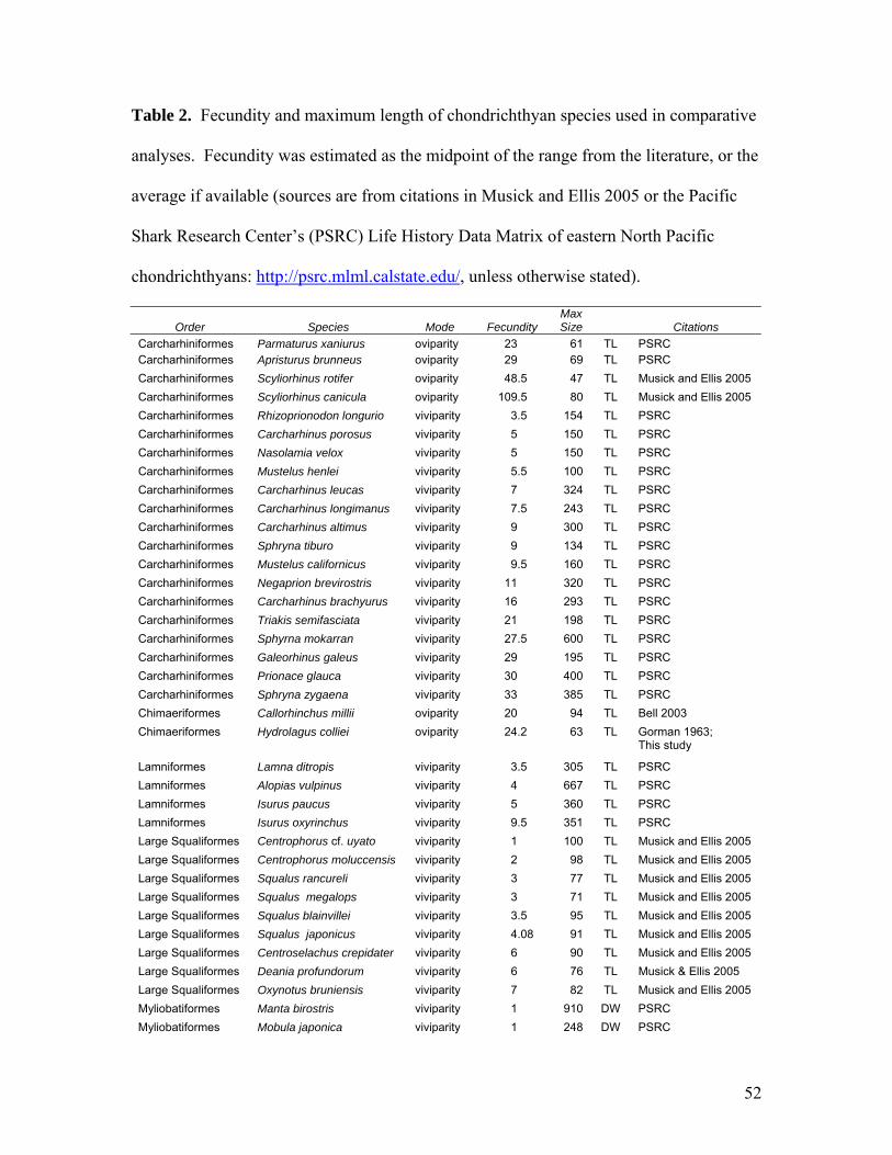
Table 2. Fecundity and maximum length of chondrichthyan species used in comparative

analyses. Fecundity was estimated as the midpoint of the range from the literature, or the

average if available (sources are from citations in Musick and Ellis 2005 or the Pacific

Shark Research Center’s (PSRC) Life History Data Matrix of eastern North Pacific

chondrichthyans: http://psrc.mlml.calstate.edu/, unless otherwise stated).

Order Species Mode Fecundity MaxSize Citations

Carcharhiniformes Parmaturus xaniurus oviparity 23 61 TL PSRC Carcharhiniformes Apristurus brunneus oviparity 29 69 TL PSRC Carcharhiniformes Scyliorhinus rotifer oviparity 48.5 47 TL Musick and Ellis 2005 Carcharhiniformes Scyliorhinus canicula oviparity 109.5 80 TL Musick and Ellis 2005 Carcharhiniformes Rhizoprionodon longurio viviparity 3.5 154 TL PSRC Carcharhiniformes Carcharhinus porosus viviparity 5 150 TL PSRC Carcharhiniformes Nasolamia velox viviparity 5 150 TL PSRC Carcharhiniformes Mustelus henlei viviparity 5.5 100 TL PSRC Carcharhiniformes Carcharhinus leucas viviparity 7 324 TL PSRC Carcharhiniformes Carcharhinus longimanus viviparity 7.5 243 TL PSRC Carcharhiniformes Carcharhinus altimus viviparity 9 300 TL PSRC Carcharhiniformes Sphryna tiburo viviparity 9 134 TL PSRC Carcharhiniformes Mustelus californicus viviparity 9.5 160 TL PSRC Carcharhiniformes Negaprion brevirostris viviparity 11 320 TL PSRC Carcharhiniformes Carcharhinus brachyurus viviparity 16 293 TL PSRC Carcharhiniformes Triakis semifasciata viviparity 21 198 TL PSRC Carcharhiniformes Sphyrna mokarran viviparity 27.5 600 TL PSRC Carcharhiniformes Galeorhinus galeus viviparity 29 195 TL PSRC Carcharhiniformes Prionace glauca viviparity 30 400 TL PSRC Carcharhiniformes Sphryna zygaena viviparity 33 385 TL PSRC Chimaeriformes Callorhinchus millii oviparity 20 94 TL Bell 2003 Chimaeriformes Hydrolagus colliei oviparity 24.2 63 TL Gorman 1963;

This study

Lamniformes Lamna ditropis viviparity 3.5 305 TL PSRC Lamniformes Alopias vulpinus viviparity 4 667 TL PSRC Lamniformes Isurus paucus viviparity 5 360 TL PSRC Lamniformes Isurus oxyrinchus viviparity 9.5 351 TL PSRC Large Squaliformes Centrophorus cf. uyato viviparity 1 100 TL Musick and Ellis 2005 Large Squaliformes Centrophorus moluccensis viviparity 2 98 TL Musick and Ellis 2005 Large Squaliformes Squalus rancureli viviparity 3 77 TL Musick and Ellis 2005 Large Squaliformes Squalus megalops viviparity 3 71 TL Musick and Ellis 2005 Large Squaliformes Squalus blainvillei viviparity 3.5 95 TL Musick and Ellis 2005 Large Squaliformes Squalus japonicus viviparity 4.08 91 TL Musick and Ellis 2005 Large Squaliformes Centroselachus crepidater viviparity 6 90 TL Musick and Ellis 2005 Large Squaliformes Deania profundorum viviparity 6 76 TL Musick & Ellis 2005 Large Squaliformes Oxynotus bruniensis viviparity 7 82 TL Musick and Ellis 2005 Myliobatiformes Manta birostris viviparity 1 910 DW PSRC Myliobatiformes Mobula japonica viviparity 1 248 DW PSRC

52


Myliobatiformes Dasyatis longa viviparity 2 156 DW Musick and Ellis 2005 Myliobatiformes Dasyatis dipterura viviparity 2.5 88 DW Musick and Ellis 2005 Myliobatiformes Urobatis halleri viviparity 2.5 18 TL PSRC Myliobatiformes Dasyatis Sabina viviparity 2.6 37 DW Musick and Ellis 2005 Myliobatiformes Aetobatus narinari viviparity 3 230 DW PSRC Myliobatiformes Dasyatis marmorata viviparity 3 440 DW Musick and Ellis 2005 Myliobatiformes Dasyatis sayi viviparity 3.5 73 DW Musick and Ellis 2005 Myliobatiformes Dasyatis centroura viviparity 4 220 DW Musick and Ellis 2005 Myliobatiformes Dasyatis tortonesei viviparity 4 80 DW Musick and Ellis 2005 Myliobatiformes Dasyatis Americana viviparity 4.2 200 DW Musick and Ellis 2005 Myliobatiformes Potamotrygon circularis viviparity 5.8 60 DW Musick and Ellis 2005 Myliobatiformes Dasyatis pastinaca viviparity 6 60 DW Musick and Ellis 2005 Myliobatiformes Dasyatis violacea viviparity 6 88 DW PSRC Myliobatiformes Potamotrygon motoro viviparity 6.3 46 DW Musick and Ellis 2005 Myliobatiformes Myliobatis californica viviparity 7 180 DW PSRC Myliobatiformes Pteroplatytrygon violacea viviparity 8.5 80 DW Musick and Ellis 2005 Myliobatiformes Gymnura marmorata viviparity 10 100 TL PSRC Orectolobiformes Hemiscyllium ocellatum oviparity 22 107 TL Compagno 2005;

Musick and Ellis 2005 Orectolobiformes Ginglymostoma cirratum viviparity 35 355 TL PSRC Rajiformes Bathyraja parmifera oviparity 29 119 TL Matta 2006 Rajiformes Leucoraja erinacea oviparity 30 54 TL Musick and Ellis 2005 Rajiformes Dipturus batis oviparity 40 250 TL Musick and Ellis 2005 Rajiformes Raja polystigma oviparity 41 53 DW Musick and Ellis 2005 Rajiformes Raja montagui oviparity 42.5 80 DW Musick and Ellis 2005 Rajiformes Amblyraja radiate oviparity 45 105 TL Musick and Ellis

2005; Sulikowski et al. 2005

Rajiformes Raja eglanteria oviparity 60 79 TL Musick and Ellis 2005 Rajiformes Raja miraletus oviparity 61 60 TL Musick and Ellis 2005 Rajiformes Raja brachyuran oviparity 65 120 TL Musick and Ellis 2005 Rajiformes Raja asterias oviparity 73 70 TL Musick and Ellis 2005 Rajiformes Leucoraja naevus oviparity 90 70 TL Musick and Ellis 2005 Rajiformes Raja clavata oviparity 100 90 TL Musick and Ellis 2005 Rhiniformes Rhyncobatus djiddensis viviparity 4 310 TL Musick and Ellis 2005 Rhinobatiformes Rhinobatos granulatus viviparity 4 280 SL Musick and Ellis 2005 Rhinobatiformes Rhinobatos hynnicephalus viviparity 4.6 44 TL Musick and Ellis 2005 Rhinobatiformes Rhinobatos lentiginosus viviparity 6 75 TL Musick and Ellis 2005 Rhinobatiformes Rhinobatos rhinobatos viviparity 7 162 TL Musick and Ellis 2005 Rhinobatiformes Rhinobatos cemiculus viviparity 7.5 230 TL Musick and Ellis 2005 Rhinobatiformes Zapteryx exasperate viviparity 7.5 97 TL Musick and Ellis 2005 Rhinobatiformes Platyrhinoides triseriata viviparity 8 91 TL Musick and Ellis 2005 Rhinobatiformes Rhinobatos horkelii viviparity 8 130 TL Musick and Ellis 2005 Rhinobatiformes Rhinobatos productus viviparity 10 156 TL PSRC Small Squaliformes Etmopterus brachyurus viviparity 2 42 TL Compagno 2005 Small Squaliformes Etmopterus hillanus viviparity 4.5 50 TL Musick and Ellis 2005 Small Squaliformes Euprotomicrus bispinatus viviparity 8 27 TL Musick and Ellis 2005 Small Squaliformes Isistius brasilliensis viviparity 9 56 TL Ebert 2003;

Compagno 2005 Small Squaliformes Etmopterus granulosus viviparity 11.5 38 TL Musick and Ellis 2005 Torpediniformes Narcine entemedor viviparity 12 93 TL PSRC Torpediniformes Torpedo californica viviparity 17 137 TL PSRC

53

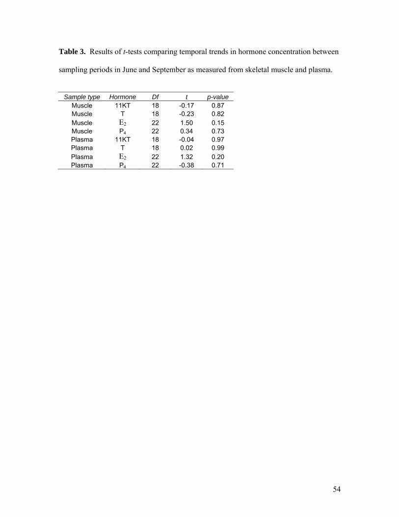
Table 3. Results of t-tests comparing temporal trends in hormone concentration between

sampling periods in June and September as measured from skeletal muscle and plasma.

Sample type Hormone Df t p-value

Muscle 11KT 18 -0.17 0.87 Muscle T 18 -0.23 0.82 Muscle E2 22 1.50 0.15 Muscle P4 22 0.34 0.73 Plasma 11KT 18 -0.04 0.97 Plasma T 18 0.02 0.99 Plasma E2 22 1.32 0.20 Plasma P4 22 -0.38 0.71

54

Table 4. Results of paired t-tests comparing hormone concentrations of skeletal muscle

sampled from the same individual immediately after capture and three hours after

capture.

Hormone df t p-value

KT 3 0.70 0.54 T 6 0.09 0.93 E2 5 0.47 0.66 P4 4 2.43 0.07

55

Figure 1. Spatial distribution of samples collected from 2003 to 2007 off California, Oregon, and Washington (between 32.6° to 48.4° N and 117.3° to 125.6° W).

56

Snout-Vent Length (mm)

0 50 100 150 200 250 300

Tota

l Wei

ght (

kg)

0.0

0.2

0.4

0.6

0.8

1.0

1.2

1.4

1.6

Figure 2. Length-weight regression for both sexes combined.

57


20 40 60 80 100 120 140 160 180 200 220

Pro

porti

onal

Inne

r Cla

sper

Len

gth

(mm

)

0.00

0.05

0.10

0.15

0.20

0.25

0.30

0.35

0.40

Figure 3. Ratio of inner clasper length to snout-vent length, displayed as a function of snout-vent length for individuals defined by the morphological criteria as juveniles (filled circles), adolescents (open circles), and adults (gray triangles).

58

Inner Clasper Length (mm)

0 10 20 30 40 50 60 70

Test

is L

engt

h (m

m)

0

10

20

30

40

50

60

Figure 4. Linear regression of inner clasper length on testis length.

59

Testis Length (mm)

0 10 20 30 40 50

Test

is W

idth

(mm

)

0

5

10

15

20

25

30

35

Figure 5. Comparison of testis length to width, displaying isometric growth of internal and external sex organs.

60

Morphological Maturity Assessment

2222222222222222222222222222222222222222222222222222222222222222222222222222222222222222222 3333333333333333333333333333333 444444444444444444444444444444444444444444444444444444444444444444444444444444444444444444444

Fron

tal T

enac

ulum

Mat

urity

Ass

essm

ent

33

22222222222222222222222222222222222222222222222222222222222222222222222222222222222222222

33333333333333333333333333333

22

44444444444444444444444444444444444444444444444444444444444444444444444444444444444444444444

3

Figure 6. Comparison of the maturity estimates made from the morphological criteria and frontal tenaculum criteria. Error bars represent 95% confidence intervals. A dotted line with a slope of one and intercept of zero is shown for reference.

61


0 50 100 150 200 250 300

Pro

porti

onal

Ovi

duca

l Gla

nd W

idth

0.00

0.02

0.04

0.06

0.08

0.10

0.12

0.14

0.16

Figure 7. Ratio of oviducal gland width to snout-vent length, displayed as a function of snout-vent length for individuals defined by the morphological criteria as juveniles (filled circles), adolescents (open circles), adults (gray triangles), and gravid adults (black triangles).

62

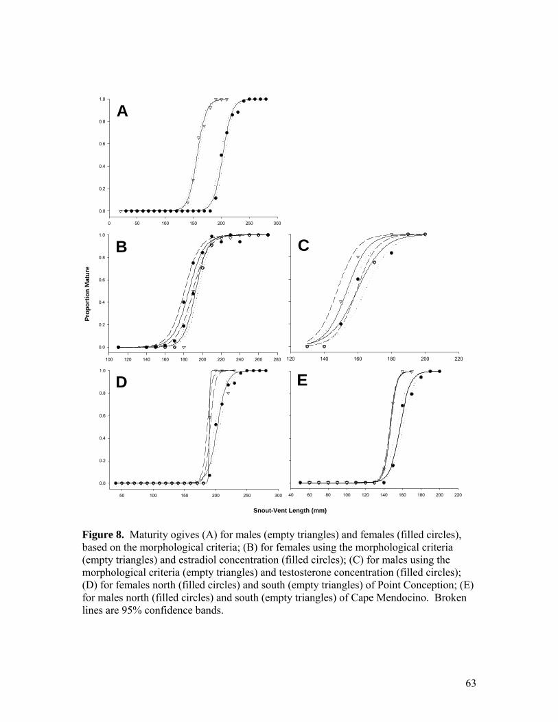
40 60 80 100 120 140 160 180 200 220


50 100 150 200 250 300

0.0

0.2

0.4

0.6

0.8

1.0

100 120 140 160 180 200 220 240 260 280

Prop

ortio

n M

atur

e

0.0

0.2

0.4

0.6

0.8

1.0

120 140 160 180 200 220

0 50 100 150 200 250 300

0.0

0.2

0.4

0.6

0.8

1.0

A

CB

ED

Figure 8. Maturity ogives (A) for males (empty triangles) and females (filled circles), based on the morphological criteria; (B) for females using the morphological criteria (empty triangles) and estradiol concentration (filled circles); (C) for males using the morphological criteria (empty triangles) and testosterone concentration (filled circles); (D) for females north (filled circles) and south (empty triangles) of Point Conception; (E) for males north (filled circles) and south (empty triangles) of Cape Mendocino. Broken lines are 95% confidence bands.

63

T (n

g/m

l)

0.0

0.1

0.2

0.3

0.4

0.5

0.6

0.0

0.1

0.2

0.3

0.4

0.5

0.6

0

10

20

30

40

50

60

70

11K

T (p

g/m

l)

0

2

4

6

8

10

12

14

June September

E2

(ng/

ml)

0.0

0.1

0.2

0.3

0.4

0.5

Month

June September0

1

2

3

4

5

6

7

P4

(ng/

ml)

0.0

0.2

0.4

0.6

0.8

1.0

0

5

10

15

20

25

Muscle Plasma

Figure 9. Comparison of mean steroid hormone concentrations from paired samples of muscle and plasma. Error bars represent 95% confidence intervals.

64

Before After

Mus

cle

E2

(ng/

ml)

0.00

0.05

0.10

0.15

0.20

0.25

0.30

0.35

Mus

cle

11K

T (p

g/m

l)

0

2

4

6

8

10

12

14

16

18

20

Mus

cle

T (n

g/m

l)

0.0

0.1

0.2

0.3

0.4

0.5

0.6

P4

(ng/

ml)

0.0

0.1

0.2

0.3

0.4

0.5

0.6

0.7

Figure 10. Comparison of mean steroid hormone concentrations from muscle sampled immediately (before) and three hours later (after). Error bars represent 95% confidence intervals.

65

Month

Jan Feb Mar Apr May Jun Jul Aug Sep Oct Nov Dec

Pro

porti

on G

ravi

d

0.00

0.02

0.04

0.06

0.08

0.10

0.12

0.14

0.16

0.18

0.20

(11) (9) (8) (10) (55) (16) (47) (56) (18) (8)(30) (1)

Figure 11. Proportion of adult females in gravid reproductive state, by month. Sample sizes are in parentheses.

66


Mat

ure

Ova

per

Fem

ale

0

5

10

15

20

25

30

35

Month(3) (0) (0) (7) (43) (9) (24) (53) (17) (0)(19) (0)

A A

B B

Figure 12. Mean number of mature ova per female, by month. Error bars represent 95% confidence intervals. Sample sizes are in parentheses. Letters indicate significant differences among months.

67


No.

Ful

ly D

evel

oped

Ova

/ Bo

dy M

ass

(g)

0.000

0.001

0.002

0.003

0.004

Month(9) (9) (8) (8) (53) (16) (46) (51) (18) (8)(29) (1)

Figure 13. Mean number of fully developed ova per female, standardized by total body mass, by month. Error bars represent 95% confidence intervals. Sample sizes are in parentheses.

68

Month


11K

T (p

g/m

L)

0

10

20

30

40

50

(1) (0) (1) (5) (34) (6) (12) (28) (10) (0)(22) (0)

A

BB

BB

BB

Figure 14. Mean female 11KT muscle concentration by month. Error bars represent 2 SEs. Sample sizes are in parentheses. Letters indicate significant differences among months.

69

Month


P4

(ng/

mL)

0

1

2

3

4

5

A

B B

(11) (2) (4) (7) (33) (6) (12) (22) (10) (5)(13) (0)

Figure 15. Mean female P4 muscle concentration by month. Error bars represent 2 SEs. Sample sizes are in parentheses. Letters indicate significant differences among months.

70

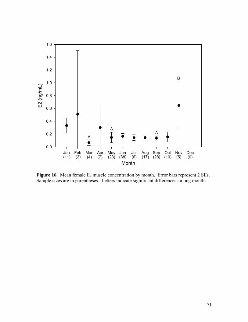
Month


E2

(ng/

mL)

0.0

0.2

0.4

0.6

0.8

1.0

1.2

1.4

1.6

B

AA

(11) (2) (4) (7) (38) (6) (17) (28) (10) (5)(23) (0)

A

Figure 16. Mean female E2 muscle concentration by month. Error bars represent 2 SEs. Sample sizes are in parentheses. Letters indicate significant differences among months.

71

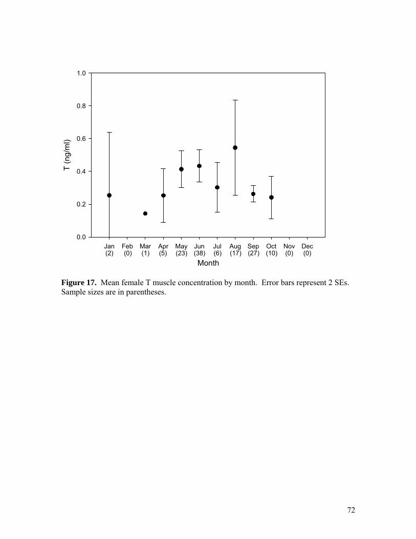
Month


T (n

g/m

l)

0.0

0.2

0.4

0.6

0.8

1.0

(2) (0) (1) (5) (38) (6) (17) (27) (10) (0)(23) (0)

Figure 17. Mean female T muscle concentration by month. Error bars represent 2 SEs. Sample sizes are in parentheses.

72


OG

I

0.000

0.005

0.010

0.015

0.020

0.025

0.030

Month(3) (1) (1) (6) (36) (8) (30) (34) (18) (0)(29) (1)

B

B BB

A

Figure 18. Mean oviducal gland index by month. Error bars represent 95 % confidence intervals. Sample sizes are in parentheses. Letters indicate significant differences among months.

73


GSI

0.00

0.01

0.02

0.03

0.04

0.05

0.06

0.07

Month(8) (9) (7) (8) (24) (13) (29) (33) (15) (6)(18) (1)

B

A

AA

Figure 19. Mean female gonadosomatic index by month. Error bars represent 95% confidence intervals. Samples sizes are in parentheses. Letters indicate significant differences among months.

74


GSI

0.00

0.01

0.02

0.03

0.04

0.05

0.06

0.07

Month(10) (8) (4) (0) (11) (9) (12) (16) (28) (3)(22) (0)

AABC

ABCABC

D CD CD

Figure 20. Mean male gonadosomatic index by month. Error bars represent 95% confidence intervals. Samples sizes are in parentheses. Letters indicate significant differences among months.

75

Somatic Weight (kg)

0.4 0.6 0.8 1.0 1.2 1.4

Num

ber o

f Ful

ly D

evel

oped

Ova

per

Fem

ale

0

2

4

6

8

10

Figure 21. Number of fully developed ova (20 mm diameter or greater) per reproductively active adult female, as a function of somatic body weight.

76


180 200 220 240 260 280 300

Max

imum

Ovu

m D

iam

eter

(mm

)

5

10

15

20

25

30

35

40

Figure 22. Maximum ovum diameter per adult female as a function of snout-vent length. Filled circles represent reproductively active individuals (those with maximum ovum diameter of 16 mm or greater), and open circles represent inactive individuals (those with maximum ovum diameter of less than 16 mm).

77

Chapter 2

Abundance and distribution

78

Introduction

Chimaeroids worldwide are captured incidentally in commercial, recreational, and

artisanal fisheries. Several chimaeroids are targeted by commercial fishermen, including

the cockfish, Callorhinchus callorhynchus, off Argentina (Di Giácomo and Perier 1991),

the elephantfish, C. milii, off New Zealand (Francis 1998), and the St. Joseph, C.

capensis, off South Africa (Freer and Griffiths 1993b). Callorhinchus milii stocks off

New Zealand were declared severely overfished in 1986, but seem to be recovering

(Francis 1998). There is not currently a directed fishery for Hydrolagus colliei, but

fishery mortality is incurred through bycatch and discard. Increasing interest in the meat

and liver oil of chimaeroids, for use as machine lubricant and human dietary supplements

(Brennan and Gormley 1999; Hardy and Mackie 1971), indicates that more chimaeroid

species may be directly harvested in the near future. As coastal and pelagic fish stocks

decrease, commercial fleets began fishing at increasing depths to obtain greater yields

(Pauly et al. 2003), increasing the likelihood of chimaeroid bycatch (Compagno and

Musick 2005).

Despite the rising interest in chimaeroid fisheries (Brennan and Gormley 1999),

there are few data regarding population status. The International Union for Conservation

of Nature Shark Specialist Group (IUCN-SSG) lists the status of all chimaeroid species

as data deficient, and stresses the need for life history information for this group (Didier

2005). There is only limited information on the impacts of fishing on chimaeroid

populations (Francis 1997; Francis 1998), as no formal population assessments have been

conducted.

79

Hydrolagus colliei is ecologically important on soft substrates of the outer shelf

and upper slope off coastal California, and the outer shelf of northern Baja California

(Allen 2006), based on relative abundance. It is one of the ten most abundant

groundfishes along the United States West Coast, between ~ 50 and 500 m depth (Keller

et al. 2006). In the nearshore waters of the Pacific Northwest it is a more substantial

component of the demersal ecosystem, as the most abundant groundfish in Puget Sound,

Washington (Palsson 2002), and in the transboundary waters of Washington and British

Columbia (Palsson et al. 2004). Despite the potential ecosystem impact of H. colliei as

predator and prey because of its sheer abundance, nothing is known of its vulnerability to

fishing mortality.

Previous authors have hypothesized that H. colliei performs movements at

multiple temporal scales (Mathews 1975; Quinn et al. 1980). Mathews (1975) suggested

that H. colliei in the northern Gulf of California underwent a seasonal migration. Quinn

et al. (1980) found evidence of seasonal movements and diel migrations in Puget Sound.

If these behaviors are typical of H. colliei populations, their susceptibility to depletion by

fisheries may be increased, as they would be more easily captured in great numbers.

I test the hypothesis that H. colliei populations along the U.S. West Coast have

decreased during the years 1977 to 2006. Fishing effort or oceanographic productivity

regimes may have caused past changes in population size. The hypothesis that

distribution varies with sex and ontogeny is tested, providing insight into how behavioral

ecology may increase the potential for population depletion. Natural mortality is

estimated using a measure of reproductive output, and age at maturity is estimated using

80

life history theory. Thus, inference is made to the resilience of the population to fishing

mortality.


Temporal and spatial trends in abundance were tested using data from the NOAA

Fisheries, Alaska Fisheries Science Center (AFSC), triennial trawl survey of groundfish

abundance from 1977 to 2004. The triennial survey varied in northern and southern

extent among years, therefore, analyses were restricted to the latitudinal range that was

surveyed in all sampling periods (36.5° to 48.5° N). Within this region, trawls were

conducted at 55 to 500 m bottom depth. Sample sites were selected randomly within

depth and latitude strata (n = 4,215; Fig. 1A). Surveys were conducted from mid-July

through September, with the exception of 2001, which was conducted from June through

August (Weinberg et al. 2002), and 2004, conducted from late May through July. Survey

vessels were chartered commercial trawlers with high-opening Nor-eastern otter trawl

nets, with rubber bobbin roller gear. Mesh size was 13 cm in trawl body, with a 9 cm

mesh codend fitted with a 3 cm liner (Weinberg et al. 1984). Tow duration was 30 min,

with a speed of ~ three knots, or 5.6 km/h (Gunderson and Sample 1980). Trawls were

conducted during daylight hours (Weinberg et al. 1984). Catch-per-unit-effort (CPUE, in

terms of no./km2 sampled) was calculated per tow by dividing the number of individuals

captured by the product of mean net width and distance fished. There were forty-two

hauls in which the catch of H. colliei was recorded only in kg. For these hauls the

number of individuals per tow was estimated by dividing the kg per tow by the average

individual mass in kg (calculated from all other hauls). Hauls identified as having little

81

or no bottom contact were removed from the analysis following the guidelines of

Zimmermann et al. (2003).

Catch-per-unit-effort was standardized with generalized linear models (GLMs),

using the ‘Delta-GLM’ function (Dick 2006) in R (version 2.4.1 for Windows). Because

the percentage of trawls with a non-zero ratfish catch varied from 32 to 62%, depending

on depth (Fig. 2), a delta-GLM approach was appropriate. The basis for the delta-GLM

approach was pioneered by Aitchison (1955) and Pennington (1983), and the method was

later modified to compare the relative abundance of fish populations through time (Lo et

al. 1992; Stefansson 1996). The delta-GLM technique uses one GLM to estimate the

probability of a positive observation using the Bernoulli probability density function and

a logit link function, and a separate GLM to estimate the mean of positive observations.

An index of abundance is then derived as the product of the year effects from the two

models. Preliminary comparisons among candidate error distributions (lognormal,

gamma, and inverse gaussian) for the positive data (following Dick 2004) provided

support for the use of the lognormal distribution. This error distribution, therefore, was

used for the positive GLM throughout subsequent analytical steps.

Selection of explanatory variables and model structure was performed using

Akaike’s Information Criterion (AIC, Akaike 1973). This information criterion was

more appropriate for model choice than hypothesis testing (likelihood ratio tests, or drop-

in-deviance-tests), because it provided a penalty term for the number of model

parameters (Akaike 1974; Burnham and Anderson 2002; Sakamoto et al. 1986), allowed

comparison of non-nested models (Hilborn and Mangel 1997), and was more robust for

analyses of large datasets (Dick 2004). Additionally, drop-in-deviance-tests are only

82

analogous to a likelihood ratio test when the dispersion parameter is equal to one, which

is not the case for the normal and gamma distribution (Venables and Dichmont 2004).

The AIC was used instead of the Bayesian Information Criterion (BIC, Schwartz 1978)

because it is more biologically realistic, considering the large amount of variance

unexplained by the “best” model (Burnham and Anderson 2002), and because the number

of potential explanatory variables was small (depth, latitude, and year). AIC scores were

compared among candidate models with backwards stepwise variable selection. Akaike

weights were calculated for each model, following Burnham and Anderson (2002):

∑ =Δ−

Δ−= R

r r

iiw

1)5.0exp(

)5.0exp(

where is the difference between the AIC scores of the ith model and the model with

the minimum AIC value, and R is the number of models compared. Using Bayesian

ideas, Akaike weights can be interpreted as estimates of the probability that model i is the

‘best’ of all included candidate models (Burnham and Anderson 2002). To facilitate

clear interpretation of results, the model structure selected by AIC for the binomial GLM

also was used for the positive GLM, even when the “best” model differed between

GLMs.

iΔ

When the model was conducted with data from the entire survey region, models

with interactions of either year and latitude or year and depth resulted in the lowest AIC

scores. To avoid these interactions, which would interfere with the interpretation of

abundance by year (Maunder and Punt 2004), the data were modeled as three separate

regions: the continental slope (250 to 500 m depth) from 36.5° to 48.5° N latitude (n =

742), and southern (36.5° to 39.5° N; n = 678) and northern (39.5° to 48.5° N; n = 2,795)

83

sections of the outer continental shelf and upper slope (50 to 250 m depth). These

geographic delineations are biologically significant, representing prominent bathymetric

(shelf break) and oceanographic (Cape Mendocino) transitions. Because of insufficient

sampling in greater depths during the years 1980 to 1992, the presence of interactions

between year and depth could not be tested for in the full slope model. A model with

truncated years (only 1977, and 1995 to 2004; Table 1A), therefore, was fitted to verify

the absence of a significant year and depth interaction. Variance estimates for the year

effect were generated with a jackknife routine to compare standardized abundances

among years. A two-step partitioning cluster analysis (Cope and Punt in review),

incorporating intra-year variance in abundance, was used to identify stock structure by

grouping model regions with similar inter-annual abundance trends.

A separate delta-GLM was created to examine the effects of coastal morphology

and oceanography on the spatial distribution of H. colliei abundance. It was possible to

include the entire latitudinal range in this model because years were lumped into three

groups (1977 to 1986, 1989 to 1992, and 1995 to 2004), based on changes in sampling

design through time (Zimmermann et al. 2003). Variance in the latitude effect was

generated with a jackknife routine to determine spatial patterns of abundance. Standard

regression diagnostics were performed for the final models to check for model

misspecification and heteroscedascity (Maunder and Punt 2004; McCullagh and Nelder

1989; Ortiz and Arocha 2004).

Data from the NOAA Fisheries, Northwest Fisheries Science Center (NWFSC),

West Coast Groundfish Survey (WCGS) were used to analyze more recent abundance

trends from 2003 to 2006. Survey methods are summarized from Keller et al. (2006), as

84

follows. Standard Aberdeen-style otter trawl nets were used, with 14 cm mesh in the

trawl body, and a 13 cm mesh codend with a 5 cm mesh liner. Footrope was composed

of rubber bobbin rollers and 25 cm dropper chains. Tow duration was ~ 15 min at ~ 2.2

knots or 4.1 km/h. Tows were conducted during daylight hours only. Surveys were

performed as two passes from the North to South between late May and mid October,

with the exception of the 2003 survey, which began in late June. Sample sites were

selected randomly within depth and latitude strata. Tows were conducted from 25 to

1,428 m, but the maximum depth of H. colliei capture was 711 m.

For the purposes of comparison, CPUE was calculated as the number of

individuals per km2 using the same technique and spatial constraints as the triennial trawl

dataset (n = 1,234; Fig. 1B). These constraints are logical, since the proportion of tows in

which ratfish were captured was minimal (0.03) between 500 m, the maximum trawl

depth of the triennial trawl survey, and 913 m, the maximum reported depth range for

ratfish. Tows conducted at depths greater than 500 m, therefore, were excluded from

abundance estimates. Similar measures also were taken to calculate standardized

abundance indices with a delta-GLM. The best fitting models as determined with AIC,

however, consistently contained interaction effects between year and depth and/or year

and latitude, regardless of the binning structure applied to explanatory variables. Because

the presence of interactions between spatial and temporal variables confounds the

interpretation of the delta-GLM year index as an indicator of temporal trends (review in

Maunder and Punt 2004), the CPUE data were simply expressed as the geometric mean

per region of the triennial trawl models. For ease of comparison, the ratio of the relative

abundances estimated by the WCGS and the triennial trawl survey for the year 2004 was

85

used to standardize the WCGS results. The geometric mean CPUE from each year and

region of the WCGS were rescaled to the GLM-standardized triennial trawl abundances

by dividing the WCGS values by x, where x = [2004 WCGS geometric mean CPUE] ÷

[2004 GLM-standardized triennial trawl CPUE].

Length-frequencies from the 2005 and 2006 NWFSC surveys (n = 682 tows with

non-zero catch; Fig. 3) were graphed separately for each sex and geographical region.

Regions were defined as the two latitudinal regions from the delta-GLM, and two

southern regions, north (34.5° to 36.5° N) and south (32.6° to 34.5° N) of Point

Conception. Tow depths were 53 to 571 m, and categorized into 100 m bins. To

determine the size selectivity of the survey, length-frequencies were recoded as

proportions of the number of individuals captured in the size class most represented in the

catch. Selectivity was then calculated by fitting a logistic equation to those data:

)*(11)( Lbae

LS +−+=

Where S(L) is the proportion of representation of size class L in the catch,

compared with the fully selected size, and parameters a and b are estimated iteratively.

From this two-year dataset, sex ratio for the entire survey area was analyzed for departure

from a 1:1 relationship using a Chi-square test. Linear least-squared regression was used

to test for differences in sex ratio with depth, with all locations pooled. ANCOVA was

used to test for latitudinal differences in the effect of depth on sex ratio, with mean

proportion of males captured per tow as the dependent variable, latitude as the main

effect, and depth as the covariate.

Qualitative observations of H. colliei distribution were made by video analysis of

visual submersible surveys conducted during August and September of 2001 and 2002, at

86

Cordell Bank, California, by the Cordell Bank National Marine Sanctuary (CBNMS).

Total size of each individual was recorded with paired lasers. Habitat type was recorded

following the classification scheme of Greene et al. (1999).

Natural Mortality

Natural mortality was estimated as a function of reproductive output (Gunderson

1997):

GSIM *79.1=

Where M is the instantaneous natural mortality rate and GSI is the estimated

annual reproductive output. A proxy for GSI was used to appropriately represent the life

history of the ratfish (after Matta 2006):

mass somatic female mature averagefecundity annual*mass ovum maximum average

=eggGSI

Where average maximum ovum mass was estimated from a subset (n = 12) of

individuals with mature ova (diameter > 20 mm), and annual fecundity was estimated

from observed laboratory parturition rates (see chapter 1 of this thesis for details). From

this estimate of natural mortality, an estimate of age at first maturity was produced, using

a rearrangement of the relationship provided by Charnov (1993):

M÷= 2α

Where α is age at first maturity, and M is natural mortality.

87

Results

Selectivity and the Distribution of ontogeny and sex

For the years 2005 and 2006 combined, for the entire survey area, the

proportion of males in the catch (0.47) was significantly less than the expected value of

0.5 (χ2 = 25.3898, df = 1, p < 0.001). In a spatially explicit context, there was a trend for

decreasing proportion of males with depth (t = 5.701, df = 678, p < 0.001). This trend,

however, was not consistent for all latitudes (ANCOVA: factor = depth*latitude, F =

1.689, df = 15, 648, p = 0.049; Fig. 4).

The size selectivity function indicated that individuals were not fully selected

until at least adult size (Fig. 5). The selectivity is likely not related to the gear, however,

because the codend mesh size was small enough to capture all ratfish, if present. If the

latter is true, size selectivity is essentially equal to one, but small individuals were

underrepresented in the size-frequency distribution because of sample site allocation,

therefore, this selectivity will be hereafter referred to as “survey selectivity”.

Length-frequency distribution appeared to vary with depth and latitude. There

was a general trend of large individuals being increasingly prevalent with decreasing

depth, with the discrepancy becoming more noticeable with increasing latitude (Fig. 6).

Trends in the shape of the distributions were similar for each sex. Absolute positions of

distributions were not compared between sexes, as females attain larger size than males.

Dense congregations of H. colliei were observed in the vicinity of Cordell Bank

(located ~ 40 km off the California coast at 38°1’42” N, 123°26’41” W). They were

patchily distributed, occurring in aggregations on the shelf break and slope around the

bank. Occasionally these aggregations were size-specific. Adult ratfish were observed

88

on the slope, at a depth of 200 to 300 m. Juvenile (possibly young-of-the-year, or YOY)

ratfish were located on the shelf break and upper slope, between 150 and 250 m. In two

consecutive years, a single transect on mud or mixed mud habitat revealed at least 50

individuals of only ~ 20 cm TL. Hundreds of H. colliei egg cases were found in the

troughs of large sand waves (~ one meter high), 60 m deep, on the continental shelf on

the eastern side of the bank.

Natural Mortality

Using the natural mortality estimation method from Gunderson (1997), with the

Matta (2006) modification, M was estimated at 0.17 to 0.26, given the range of fecundity

estimates. The estimated range of M provides an expected age at first maturity of 7.8 to

11.6 years.

Spatial and Temporal Abundance Trends

The models that best predicted the probability of catching at least one ratfish, and

the catch rate, varied among regions (Table 1). The slope model with truncated years

indicated the absence of a year and depth interaction (Table 1A), therefore, the slope

model with all years included (and no year and depth interaction) was used for inferring

temporal abundance trends. The models selected to create temporal and spatial indices of

abundance are as follows:

89

1) Slope: year, latitude (2 degree bins), depth (62 m bins)

2) Northern shelf and upper slope: year, latitude (1 degree bins), depth (50 m bins),

depth * latitude

3) Southern shelf and upper slope: year, latitude (1 degree bins), depth (67 m bins),

depth * latitude

4) Entire survey region: year (1977 to 1986, 1989 to 1992, 1995 to 2004), latitude

(0.5 degree bins)

The models fit the positive data reasonably well (see appendix), with R2 values of

0.201, 0.125, 0.151, and 0.111, respectively. Cluster analysis indicated that the temporal

abundance trends were similar between the slope, and northern shelf and upper slope

populations (Sil = 0.95), but differed for the southern shelf and upper slope population.

The slope model indicated a consistent increase in abundance since 1995, with the

exception of 2001 (Fig. 7A). The same trend was even more dramatic in the northern

shelf and upper slope region (Fig. 7B). Abundance trends in the southern shelf and upper

slope region were not as straightforward, with increasing abundance from 1977 to 1986,

and lesser abundance thereafter, with the exception of a large peak in 1995 (Fig. 7C).

The model created to determine spatial trends in abundance included only the

main effects of two explanatory variables: year (grouped), and latitude (0.5 degree bins).

Standardized abundance (Fig. 8) was greater off Cape Flannery (48.0 to 48.5° N),

Monterey Bay (36.5 to 37.0° N), and just south of Cape Mendocino (40.0 to 40.5° N).

Abundance was less near the Columbia River Plume (44.5 to 45.5° N), between Cape

90

Mendocino and Cape Blanco (40.5 to 42.0° N), and just south of San Francisco Bay (37.0

to 37.5° N).

Discussion

Selectivity and the Distribution of ontogeny and sex

The phenomenon of sexual segregation by depth occurs in many elasmobranch

populations (e.g. Compagno et al. 1991). In this study, sex ratio became more skewed

toward females with depth across most of the geographic range, similar to the pattern

observed for the black dogfish, Centroscyllium fabricii (Yano 1995) and the marbled

catshark, Galeus arae (Bullis 1967). The reasons for this type of sexual segregation

remain unknown. This result, however, may be an artifact of size selectivity of sampling

(Fig. 5). Survey catch may be biased toward females, because males reach a smaller size

at maturity and lesser maximum size than females.

Visual analysis of length-frequency distributions indicated that the prevalence

of large individuals decreased with depth (Fig. 6). This trend, however, may be an

artefact of sampling design, as the number of trawl samples decreased with depth. The

length-frequencies of deeper areas, therefore, may not be representative of the true size

structure.

Ontogenetic segregation by habitat type can be inferred from the size selectivity

of the survey, wherein only adults were sufficiently sampled. Absolute biomass

estimates derived from the triennial trawl survey would therefore be an underestimate.

The disproportionately lesser number of juveniles in the catch indicated that they may be

associated with rocky habitats that are not easily sampled with trawl gear. Visual

91

observations of aggregations of juveniles on soft-bottom habitats around Cordell Bank

provide evidence against the latter hypothesis, perhaps indicating that the dearth of

juveniles in the catch may be caused by vertical movements. Submersible observations at

Stonewall Bank revealed an abundance of ratfish at night, but an absence during the day

(Hixon and Tissot 1992), providing more evidence for the phenomenon of vertical

movements.

The presence of aggregations of egg cases and juveniles near the shelf break,

adjacent to Cordell Bank, indicate that this may be a nursery area for H. colliei. Egg case

deposition also has been observed on Daisy Bank, ~ 56 km west of Newport, Oregon

(Mark Hixon, pers. comm.). These observations indicate offshore banks may be nursery

areas for H. colliei, as they are for many species of rockfish (Pearcy et al. 1989).

The wave formations in the sandy habitat where the egg cases were found would

indicate that there are high-velocity currents propagating near the seafloor in this region.

Aggregations of egg-cases of the catsharks Apristurus brunneus and Parmaturus

xaniurus have also been found at the shelf break and upper slope interface in regions with

strong seafloor currents (Flammang 2005). The shelf break is a nursery area for many

species, including Scyliorhinus retifer (Able and Flescher 1991). Ridges with strong

currents are nursery areas for some deep-sea teleosts and cephalopods (Drazen et al.

2003). Flammang (2005) indicated that the currents were needed to provide oxygenated

water for egg cases.

Alternative reasons for the selective deposition of egg cases into sand troughs

may be to reduce egg case mortality by avoiding predator-dense habitats, and to prevent

passive transport of the unborn offspring to less favorable habitats. There also may be

92

increased food abundance for juveniles near offshore banks, but Heupel et al. (2007)

noted that chondrichthyan nursery areas typically function more to decrease early life

history mortality than to increase food availability. The existence of nursery areas may

increase the vulnerability of the species to population depletion by potentially increasing

the mortality of immature individuals (through fisheries catch), the most important vital

rate contributing to population growth in chondrichthyans (Cortes 2002; Frisk et al.

2005).

Natural Mortality

The estimated natural mortality of 0.17 to 0.26 is slightly less than the median of

0.27 calculated from 55 species of elasmobranchs (review in Frisk et al. 2005). The

estimated age at first maturity of 7.8 to 11.6 was similar to, if not slightly greater than,

the female-specific median of 8 years calculated using 68 shark populations (review in

Cortes 2000). It should be noted, however, that estimates for H. colliei were indirectly

derived, and should be interpreted with caution.

Spatial and Temporal Abundance Trends

Populations on the slope and the northern region of the shelf and upper slope have

greatly increased since 1998. No such increase, however, was observed for the southern

shelf and upper slope population. Probable causes of this geographic variation are

climate and differential fishing mortality.

Temporal trends in abundance of many U.S. West Coast groundfishes have been

attributed to fluctuations in fishing mortality, with landings used as a proxy for this

93

factor. Levin et al. (2006) reported changes in the benthic fish assemblage off the U.S.

West Coast, with abundances of many rockfish species decreasing, and all flatfish and

chondrichthyan species increasing. Size at maturity, maximum size, and individual

growth rate, were also associated with population growth rate. Abundance trends were

inversely associated with landings, indicating that fishing mortality was a contributing

factor to decreasing population size of rockfishes.

To assess the temporal and spatial effects of fishing on H. colliei populations,

U.S. West Coast groundfish landings were compared with the spatially explicit

abundance trends. Annual landings from all gear types in the U.S. West Coast

groundfish fisheries increased steadily from 1985 to 1989, then remained above 200,000

mt before decreasing in 2002 and 2003 to record mimima since accounting began by the

Pacific Fishery Management Council (PFMC) Groundfish Management Team in 1981

(Fig. 9; PacFIN 2008). Beginning in 2003, the PFMC enacted new management

procedures, most notably closing specific depth zones of the continental shelf to trawling

and reducing catch limits of certain species. With fishing effort concentrated on the

deeper waters of the continental slope and outer shelf, groundfish landings have since

increased, before a decline in 2007. These trends in fishing effort, inferred by landings,

do not coincide with H. colliei abundance trends. Fishing mortality, therefore, is not the

primary factor regulating H. colliei abundance in space or time.

Levin et al. (2006) reported on the influence of harvest on population size, but

concurrent climate influences were not addressed. A strong El Niño occurred between

1997 and 1998, and a shift to a cold regime of the Pacific Decadal Oscillation (PDO) may

have occurred around the same time. These cold regimes provide more nutrient-rich

94

water to the California Current System (CCS), promoting greater primary productivity,

which may increase the abundance of benthic epifauna and infauna that H. colliei prey

upon (Johnson and Horton 1972). Increased food availability may allow H. colliei

population size to increase during cold regimes.

The increased abundance in the slope population in 1983 and 1998, relative to

adjacent survey years, indicated that El Niño conditions may cause H. colliei populations

to move to deeper waters. Exceptionally strong El Niño events occurred between 1982

and 1983, and 1997 and 1998. El Niño events cause a depression in depth of the surface

mixed layer (Simpson 1984; Zimmerman and Kremer 1984; Zimmerman and Robertson

1985). The mixed layer contains nutrient depleted, warm water during such anomalies

(Eppley et al. 1979; Jackson 1977; Zimmerman and Kremer 1984). These movements,

therefore, likely are caused by a depression of the thermocline and nutricline.

Hydrolagus colliei has a shallow depth distribution, relative to other chimaeroids.

Within the latitudinal extent of the range surveyed, they were most prevalent at depths of

150 to 400 m (Fig. 2). As previously hypothesized (Dean 1906), their abundance

decreased with depth at higher latitudes, but this relationship gradually degraded toward

the lower latitudes (Fig. 10), perhaps explaining the model interactions between depth

and latitude. This pattern is a common biogeographical phenomenon of many marine

species, and typically is attributed to the bathymetric distribution of thermal isoclines.

Tolimieri and Levin (2006), however, found that although bottom temperature decreases

with depth and latitude on the U.S. West Coast, spatial variation of fish assemblage

structure was not fully explained temperature alone. Assemblage structure within the

depths 200 to 500 m changed in the vicinity of Cape Mendocino and Point Conception, a

95

similar pattern to that of nearshore fishes (SCCWRP 1973), with less drastic shifts around

Cape Blanco and the Columbia River plume.

Intraspecific population structure of H. colliei may be produced by physical

factors similar to those which structure demersal fish communities, as they seem to share

some geographical boundaries. Anomalously lesser and greater densities were observed

across all depths at specific latitudinal regions (Fig. 8). Such anomalies may be caused

by variability in the strength of currents at the seafloor, seafloor habitat and relief, prey

abundance, or aggregative behavior. Regions with greater ratfish abundance (36.5 to

37.0°, 40 to 40.5°, 48.0 to 48.5° N) corresponded with the prominent coastal physical

features of Monterey Bay, Cape Mendocino, and Cape Flannery. These areas are

exceedingly productive, as their coastal morphology increases the amount of localized

upwelling, therefore increasing the rate of primary productivity.

Increased primary productivity at the sea surface may provide more nutrients to

benthic infauna and epifauna, thus providing a greater abundance of prey for H. colliei,

which feed primarily on shrimp (Pandalus sp. and Crago sp.), echinoderms (Brisaster

sp.), and gastropod mollusks (Johnson and Horton 1972). The lesser density of H. colliei

between Cape Mendocino and Cape Blanco (40.5 to 42.0° N) may be caused by lesser

food abundance relative to these adjacent highly productive upwelling regions formed by

the two coastal promontories (NOAA 2008). Lesser H. colliei abundances near the

Columbia River plume (~45.0° N), and just south of San Francisco Bay (~37.5° N),

cannot be explained as easily.

This pattern of decreased abundance is somewhat counterintuitive, because these

are areas of great runoff, therefore, one would expect increased abundance of their

96

benthic macrofaunal prey, as coastal runoff contains greater nutrient levels than coastal

marine waters (Bakun 1996). Eutrophic plumes with high sediment loads, however, can

create anoxic conditions on the seafloor, which can cause population depletion of benthic

invertebrates (Baden et al. 1990) and fishes (Mellergaard and Nielsen 1990).

Additionally, there may be strong currents on the seafloor in these regions, as evidenced

by large sand waves at the mouth of San Francisco Bay (Barnard et al. 2006), perhaps

deterring the relatively small-bodied ratfish. Combes and Daniel (2001) reported that

maximum sustained swimming speed of H. colliei was only 0.15 ms-1, consequently, they

may not be able to inhabit areas with strong currents for protracted time periods.

The latitudinal population structure may indicate the presence of intraspecific

phylogenetic barriers. Hydrolagus colliei should be expected to display strong

population structure because it has no embryonic dispersal, and unknown levels of

juvenile and adult dispersal. Combes and Daniel (2001), however, noted that flexibility

of the pectoral fins of H. colliei allows for increased efficiency, which indicates that adult

dispersal potential could be greater than previously thought. Cape Mendocino is an

intraspecific phylogeographic break for some fishes (Cope 2004; Dawson et al. 2001).

Anomalously lesser ratfish abundance just north of this coastal promontory, combined

with the evidence of differing temporal abundance trends within populations to the north

and south, indicates that it may play a similar role for this species.

Conclusions

The life history, movement patterns, and aggregative behavior of H. colliei

indicate that it may be vulnerable to population depletion by excess fisheries mortality.

97

Temporal abundance trends, however, indicate that their population size has increased

significantly within the last decade. It is unclear whether this increase was caused by the

success of fisheries management policy, or shifting regimes of oceanographic

productivity increasing their abundance and/or availability to fishing gear. It is evidence,

nonetheless, of the resilience of this species to increased mortality from anthropogenic

and environmental sources. The paradigm that all chondrichthyans are particularly

susceptible to exploitation, therefore, may not apply to chimaeroids.

98

Literature Cited

Able KW, Flescher D (1991) Distribution and habitat of chain dogfish, Scyliorhinus

retifer, in the Mid Atlantic bight. Copeia 1: 231-234

Aitchison J (1955) On the distribution of a positive random variable having a discrete

probability mass at the origin. Journal of the American Statistics Association 50:

901-908

Akaike H (1973) Information theory and an extension of the maximum likelihood

principle. In: Petrov BN, Csaki F (eds) Proceedings of the 2nd international

symposium on information theory. Publishing House of the Hungarian Academy

of Sciences, Budapest, pp 268-281

Akaike H (1974) A new look at the statistical model identification. IEEE Transactions on

Automatic Control AC-19: 716-723

Allen MJ (2006) Continental shelf and upper slope. In: Allen MJ, Pondella DJ, II, Horn

MH (eds) The Ecology of Marine Fishes: California and Adjacent Waters.

University of California Press, Berkeley, CA

Baden SP, Loo LO, Pihl L, Rosenberg R (1990) Effects of eutrophication on benthic

communities including fish: Swedish west coast. Ambio 19: 113-122

Bakun A (1996) Patterns in the ocean: ocean processes and marine population dynamics.

University of California Sea Grant (in cooperation with Centro de Investigaciones

Biologicas de Noroeste, La Paz, Baja California Sur, Mexico), San Diego,

California, USA

Barnard PL, Hanes DM, Rubin DM, Kvitek RG (2006) Giant sand waves at the mouth of

San Francisco Bay. Eos, AGU 87: 285, 289

99

Brennan MH, Gormley TR (1999) The quality of under-utilised deep-water fish species.

Teagasc Research Report 22 (Project Armis No. 4560)

Bullis HRJ (1967) Depth segregations and distribution of sex-maturity groups in the

marbled catshark, Galeus arae. In: Gilbert PW, Mathewson RF, Rall DP (eds)

Sharks, Skates, and Rays. The Johns Hopkins Press, Baltimore, pp 141-148

Burnham KP, Anderson DR (2002) Model Selection and Multimodel Inference: A

Practical Information-Theoretic Approach. Spinger-Verlag, New York

Charnov EL (1993) Life History Invariants: Some Explorations of Symmetry in

Evolutionary Ecology. Oxford University Press, Inc., New York

Combes SA, Daniel TL (2001) Shape, flapping and flexion: wing and fin design for

forward flight. The Journal of Experimental Biology 204: 2073-2085

Compagno LJV, Ebert DA, Cowley PD (1991) Distribution of offshore demersal

cartilaginous fish (Class Chondrichthyes) off the west coast of Southern Africa,

with notes on their systematics. South African Journal of Marine Science 11: 43-

139

Compagno LJV, Musick JA (2005) Deepwater species. In: Fowler SL, Cavanaugh RD,

Camhi M, Burgess GH, Cailliet GM, Fordham SV, Simpfendorfer CA, Musick JA

(eds) Sharks, rays and chimaeras: the status of the chondrichthyan fishes. Status

Survey. IUCN/SSC Shark Specialist Group. IUCN, Gland, Switzerland and

Cambridge, UK, pp 216-217

Cope JM (2004) Population genetics and phylogeography of the blue rockfish (Sebastes

mystinus) from Washington to California. Canadian Journal of Fisheries and

Aquatic Sciences 61: 332-342

100

Cope JM, Punt AE (in review) Drawing the lines: Resolving fishery management units

with simple fisheries data. Canadian Journal of Fisheries and Aquatic Sciences

Cortes E (2000) Life history patterns and correlations in sharks. Reviews in Fisheries

Science 8: 299-344

Cortes E (2002) Incorporating uncertainty into demographic modeling: Application to

shark populations and their convervation. Conservation Biology 16: 1048-1062

Dawson MN, Staton JL, Jacobs DK (2001) Phylogeography of the tidewater goby,

Eucyclogobius newberryi (Teleostei, Gobiidae), in coastal California. Evolution

55(6): 1167-1179

Dean B (1906) Chimaeroid fishes and their development. Carnegie Institute Publication,

Washington, D.C.

Di Giácomo EE, Perier MR (1991) Evaluación de la biomasa y explotación comercial de

pez gallo (Callorhynchus Callorhynchus) en el golfo San Matías, Argentina.

Frente Maritimo 9: 7-13

Dick EJ (2004) Beyond `lognormal versus gamma': discrimination among error

distributions for generalized linear models. Fisheries Research 70: 351-366

Dick EJ (2006) Delta-GLM. Version 1.7.2, Programmed in R version 2.2 for Windows

Didier DA (2005) Order chimaeriformes, chimaeras. In: Fowler SL, Cavanaugh RD,

Camhi M, Burgess GH, Cailliet GM, Fordham SV, Simpfendorfer CA, Musick JA

(eds) Sharks, rays and chimaeras: the status of the chondrichthyan fishes. Status

survey. IUCN/SSC Shark Specialist Group, IUCN, Gland, Switzerland and

Cambridge, UK

101

Drazen JC, Goffredi SK, Schlining B, Stakes DS (2003) Aggregations of egg-brooding

deep-sea fish and cephalopods on the gorda escarpment: a reproductive hot spot.

Biological Bulletin 205: 1-7

Eppley RW, Renger EH, Harrison WG (1979) Nitrate and phytoplankton production in

Southern California Coastal Waters. Limnology and Oceanography 24: 483-494

Flammang BE (2005) Distribution and reproductive ecology of deep-sea catsharks

(Chondrichthyes: Scyliorhinidae) of the eastern North Pacific. M.S. Thesis, Moss

Landing Marine Laboratories

Francis MP (1997) Spatial and temporal variation in the growth rate of elephantfish

(Callorhinchus milii). New Zealand Journal of Marine and Freshwater Research

31: 9-23

Francis MP (1998) New Zealand shark fisheries: development, size and management.

Marine and Freshwater Research 49: 579-591

Freer DWL, Griffiths CL (1993) The fishery for, and general biology of, the St. Joseph

Callorhinchus capensis (Dumeril) off the southwestern Cape, South Africa. South

African Journal of Marine Science 13: 63-74

Frisk MG, Miller TJ, Dulvy NK (2005) Life histories and vulnerability to exploitation of

elasmobranchs: inferences from elasticity, perturbation and phylogenetic

analyses. Journal of Northwest Atlantic Fishery Science 35: 27-45

Greene GH, Yoklavich MM, Starr RM, O'Connell VM, Wakefield WW, Sullivan DE,

McRea Jr. JE, Cailliet GM (1999) A classification scheme for deep seafloor

habitats. Oceanologica Acta 22: 663-678

102

Gunderson DR (1997) Trade-off between reproductive effort and adult survival in

oviparous and viviparous fishes. Canadian Journal of Fisheries and Aquatic

Sciences 54: 990-998

Gunderson DR, Sample TE (1980) Distribution and abundance of rockfish off

Washington, Oregon, and California during 1977. Marine Fisheries Review 42: 2-

16

Hardy R, Mackie PR (1971) Observations on the chemical composition and toxicity of

ratfish (Chimaera monstrosa). Journal of the Science of Food and Agriculture 22:

382-388

Heupel MR, Carlson JK, Simpfendorfer CA (2007) Shark nursery areas: concepts,

definition, characterization and assumptions. Marine Ecology Progress Series

337: 287-297

Hilborn R, Mangel M (1997) The Ecological Detective: Confronting Models with Data.

Princeton University Press, Princeton, NJ

Hixon MA, Tissot BN (1992) Fish Assemblages of Rocky Banks of the Pacific

Northwest [Stonewall Bank]. A final report supplement by the Department of

Zoology of Oregon State University for the U.S. Department of the Interior,

Minerals Management Service Pacific OCS Office, Camarillo, CA

Jackson GA (1977) Nutrients and production of giant kelp, Macrocystis pyrifera, off

southern California. Limnology and Oceanography 22: 979-995

Johnson AG, Horton HF (1972) Length-weight relationship, food habits, parasites, and

sex and age determination of the ratfish, Hydrolagus colliei (Lay and Bennett).


103

Keller AA, Horness BH, Tuttle VJ, Wallace JR, Simon VH, Fruh EL, Bosley KL,

Kamikawa DJ (2006) The 2002 U.S. West Coast upper continental slope trawl

survey of groundfish resources off Washington, Oregon, and California:

Estimates of distribution, abundance, and length composition. U.S. Department of

Commerce, NOAA Technical Memorandum, NMFS-NWFSC-75

Levin PS, Holmes EE, Piner KR, Harvey CJ (2006) Shifts in a Pacific Ocean fish

assemblage: the potential influence of exploitation. Conservation Biology 20:

1181-1190

Lo NCH, Jacobson ID, Squire JL (1992) Indices of relative abundance from fish spotter

data based on delta-lognormal models. Canadian Journal of Fisheries and Aquatic

Sciences 49: 2515-2526

Mathews CP (1975) Note on the ecology of the ratfish, Hydrolagus collei, in the Gulf of

California. California Fish and Game 61: 47-53

Matta EM (2006) Aspects of the life history of the Alaska skate, Bathyraja parmifera, in

the eastern Bering Sea. M.S. Thesis, University of Washington, Seattle

Maunder MN, Punt AE (2004) Standardizing catch and effort data: a review of recent

approaches. Fisheries Research 70: 141-159

McCullagh P, Nelder JA (1989) Generalized Linear Models. Chapman and Hall, New

York

Mellergaard S, Nielsen E (1990) Fish disease investigations in Danish coastal waters with

special reference to the impact of oxygen deficiency. ICES C.M. E6: 1-21

NOAA CP (2008) Sea-viewing Wide Field-of-view Sensor (SeaWiFS) Sea Surface

Chlorophyll-a Concentration, West U.S., 0.036 degree latitude resolution. Data

104

courtesy of NASA/GSFC/DAAC, GeoEye. Data accessed through the

OceanWatch server http://las.pfeg.noaa.gov/oceanWatch/oceanwatch_safari.php,

developed at the Environmental Research Division, Southwest Fisheries Science

Center, National Marine Fisheries Service, NOAA.

Ortiz M, Arocha F (2004) Alternative error distribution models for standardization of

catch rates of non-target species from a pelagic longline fishery: billfish species in

the Venezuelan tuna longline fishery. Fisheries Research 70: 275-297

PacFIN (2008) PFMC Port Group Report: Groundfish Landed-catch (Metric tons) for All

Gears. http://www.psmfc.org/pacfin/pfmc.html. Accessed January 7, 2008.

Palsson WA (2002) Survey-based stock trends for Puget Sound groundfishes: Monitoring

the road to recovery. Puget Sound Research 2001. Puget Sound Action Team,

Olympia, Washington

Palsson WA, Beam J, Hoffmann S, Clarke P (2004) Fish without borders: trends in the

status and distribution of groundfish in the transboundary waters of Washington

and British Columbia. In: Droscher TW, Fraser DA (eds) Proceedings of the 2004

Georgia Basin/Puget Sound Research Conference

Pauly D, Alder J, Bennett E, Christensen V, Tyedmers P, Watson R (2003) The future of

fisheries. Science 302: 1359-1361

Pearcy WG, Stein DL, Hixon MA, Pikitch EK, Barss WH, Starr RM (1989) Submersible

observations of deep-reef fishes of Heceta Bank, Oregon. Fishery Bulletin 87:

955-965

Pennington M (1983) Efficient estimators of abundance, for fish and plankton surveys.

Biometrics 39: 281-286

105

http://las.pfeg.noaa.gov/oceanWatch/oceanwatch_safari.php

http://www.psmfc.org/pacfin/pfmc.html

Quinn TP, Miller BS, Wingert RC (1980) Depth distribution and seasonal and diel

movements of ratfish, Hydrolagus colliei, in Puget Sound, Washington. Fishery

Bulletin 78: 816-821

Sakamoto Y, Ishiguro M, Kitagawa G (1986) Akaike Information Statistics. KTK

Scientific Publishers, Tokyo, and D. Reidel Publishing, Dordrecht

SCCWRP (1973) The ecology of the Southern Californian bight: implications for water

quality management. El Segundo, California. Southern California Coastal Water

Research Project, Technical Report 104

Schwartz G (1978) Estimating the dimension of a model. Annals of Statistics 6: 461-464

Simpson JJ (1984) El Niño-induced onshore transport in the California current during

1982-1983. Geophysical Research Letters 11: 241-242

Stefansson G (1996) Analysis of groundfish survey abundance data: combining the GLM

and delta approaches. ICES Journal of Marine Science 53: 577-588

Tolimieri N, Levin PS (2006) Assemblage structure of eastern Pacific groundfishes on

the U.S. continental slope in relation to physical and environmental variables.

Transactions of the American Fisheries Society 135: 317-332

Venables WN, Dichmont CM (2004) GLMs, GAMs and GLMMs: an overview of theory

for applications in fisheries research. Fisheries Research 70: 319-337

Weinberg KL, Wilkins ME, Dark TA (1984) The 1983 Pacific west coast bottom trawl

survey of groundfish resources: estimates of distribution, abundance, age and

length composition. U.S. Department of Commerce, NOAA Technical

Memorandum NMFS F/NWC-70

106

107

Weinberg KL, Wilkins ME, Shaw FR, Zimmerman FR (2002) The 2001 Pacific West

Coast bottom trawl survey of groundfish resources: Estimates of distribution,

abundance, and length and age composition. U.S. Department of Commerce,

NOAA Technical Memorandum NMFS-AFSC-128

Yano K (1995) Reproductive biology of the black dogfish, Centroscyllium fabricii,

collected from waters off western Greenland. Journal of the Marine Biological


Zimmerman RC, Kremer JN (1984) Episodic nutrient supply to a kelp forest ecosystem

in southern California. Journal of Marine Research 42: 591-604

Zimmerman RC, Robertson DL (1985) Effects of El Niño on local hydrography and

growth of the giant kelp, Macrocystis pyrifera, at Santa Catalina Island,

California. Limnology and Oceanography 30: 1298-1302

Zimmermann M, Wilkins ME, Weinberg KL, Lauth RR, Shaw FR (2003) Influence of

improved performance monitoring on the consistency of a bottom trawl survey.

ICES Journal of Marine Science 60: 818-826

Table 1. Model selection criteria for each delta-GLM, sorted by AIC score of the binomial fit. Final models are in bold.

Binomial Lognormal Model structure df AIC ΔAIC Akaike AIC ΔAIC Akaike weights Weights (A) Slope with years truncated Year + Latitude + Depth + Year:Latitude + Depth:Latitude + Year:Depth 59 733.44 24.34 0.00 945.45 25.60 0.00 Year + Latitude + Depth + Year:Latitude + Depth:Latitude 47 719.94 10.84 0.00 926.37 6.52 0.04 Year + Latitude + Depth + Depth:Latitude 27 714.62 5.52 0.06 925.80 5.95 0.05 Year + Latitude + Depth 12 709.10 0.00 0.94 919.85 0.00 0.92 Latitude + Depth 8 740.02 30.92 0.00 939.60 19.75 0.00 Latitude 5 761.50 52.40 0.00 947.70 27.85 0.00 1 1 797.60 88.50 0.00 966.30 46.45 0.00 (B) Slope Year + Latitude + Depth + Year:Latitude + Depth:Latitude 76 963.92 18.57 0.00 1225.29 17.65 0.00 Year + Latitude + Depth + Depth:Latitude 32 946.98 1.63 0.31 1212.24 4.60 0.09 Year + Latitude + Depth 17 945.35 0.00 0.69 1207.64 0.00 0.91 Latitude + Depth 8 978.92 33.57 0.00 1221.18 13.54 0.00 Latitude 5 997.10 51.75 0.00 1232.00 24.36 0.00 1 1 1031.00 85.65 0.00 1256.00 48.36 0.00 (C) Northern shelf and upper slope Year + Latitude + Depth + Year:Latitude + Depth:Latitude + Year:Depth 143 3611.35 30.91 0.00 4329.52 53.57 0.00 Year + Latitude + Depth + Year:Latitude + Depth:Latitude 116 3591.95 11.51 0.00 4305.10 29.15 0.00 Year + Latitude + Depth + Depth:Latitude 44 3580.44 0.00 1.00 4286.91 10.96 0.00 Year + Latitude + Depth 20 3631.00 50.56 0.00 4275.95 0.00 1.00 Latitude + Depth 11 3748.00 167.56 0.00 4304.20 28.25 0.00 Latitude 8 3776.00 195.56 0.00 4308.00 32.05 0.00 1 1 3876.00 295.56 0.00 4383.00 107.05 0.00 (D) Southern shelf and upper slope Year + Latitude + Depth + Year:Latitude + Depth:Latitude + Year:Depth 53 854.99 31.17 0.00 882.09 26.84 0.00 Year + Latitude + Depth + Year:Latitude + Depth:Latitude 35 839.04 15.22 0.00 861.88 6.63 0.02 Year + Latitude + Depth + Depth:Latitude 17 823.82 0.00 0.80 856.55 1.30 0.33 Year + Latitude + Depth 13 826.57 2.75 0.20 855.25 0.00 0.64 Latitude + Depth 4 877.20 53.38 0.00 872.70 17.45 0.00 Latitude 2 873.20 49.38 0.00 872.00 16.75 0.00 1 1 921.30 97.48 0.00 868.50 13.25 0.00 (E) Entire survey area with years grouped YearGrouped + Latitude + YearGrouped:Latitude 71 5521.10 2.50 0.22 6355.88 20.45 0.00 YearGrouped + Latitude 25 5518.60 0.00 0.78 6335.43 0.00 1.00 Latitude 23 5623.30 104.70 0.00 6353.50 18.07 0.00 1 1 5839.00 320.40 0.00 6522.00 186.57 0.00

108

Figure 1. Start-of-haul locations for (A) the AFSC triennial trawl surveys (1977 to 2004), and (B) the NWFSC West Coast Groundfish Surveys (2003 to 2006). Samples shown here are those restricted to the latitudinal range used for abundance analysis (36.5° to 48.5° N).

A B

109

Depth (m)

0 100 200 300 400 500

Pro

porti

on P

ositi

ve T

ows

0.0

0.1

0.2

0.3

0.4

0.5

0.6

0.7

Figure 2. Proportion of positive tows by 50 m depth bin (each bin comprises 50 m from

the given x-axis label).

110

Figure 3. Start-of-haul locations for the 2005 and 2006 NWFSC West Coast Groundfish Surveys. Hauls with zero catch are in grey and those with positive catch are in black.

111

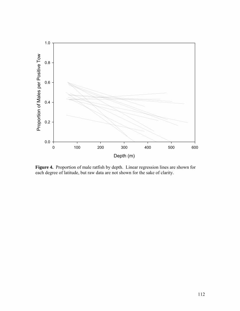
Depth (m)

0 100 200 300 400 500 600

Prop

ortio

n of

Mal

es p

er P

ositi

ve T

ow

0.0

0.2

0.4

0.6

0.8

1.0

Figure 4. Proportion of male ratfish by depth. Linear regression lines are shown for each degree of latitude, but raw data are not shown for the sake of clarity.

112

Snout-Vent Length (cm)

0 10 20 30

Ret

entio

n Pr

obab

ility

0.0

0.2

0.4

0.6

0.8

1.0

Figure 5. Survey selectivity function for the NWFSC West Coast Groundfish Survey, from the years 2005 and 2006 (n = 7,020).

113

Males Females

Figure 6. Length-frequencies by depth for males and females between the latitudinal regions (A) 39.5° to 48.5° N, (B) 36.5° to 39.5° N, (C) 34.5° to 36.5° N, and (D) 32.6° to 34.5° N.

A

B

C

D

Freq

uenc

y

5

10

15

20

25

Snout-Vent Length (cm

)50

150

250

350

450

550

Depth (m)

80

160

240

320

5

10

15

20

25

50

150

250

350

450

550

80

160

240

320

5

10

15

20

25

50

150

250

350

450

550

80

160

240

320

5

10

15

20

25

50

150

250

350

450

550

80

160

240

320

5

10

15

20

25

Snout-Vent Length (cm

)50

150

250

350

450

550

Depth (m)

80

60

240

320

1

5

10

15

20

25

50

150

250

350

450

550

80

160

240

320

5

10

15

20

2550

150

250

350

450

550

80

160

240

320

5

10

15

20

25

50

150

250

350

450

550

80

160

240

320

114

0

200

400

600

800

CP

UE

(# in

divi

dual

s/km

2 )

0

100

200

300

400

500

Year

1977 1980 1983 1986 1989 1992 1995 1998 2001 2004 20070

50

100

150

200

250

300

A

B

C

Figure 7. GLM-standardized CPUE estimates from the continental slope (250 to 500 m depth) between the latitudes of 36.5° to 48.5° N (A), the continental shelf and upper slope (50 to 250 m depth) between the latitudes of 39.5° to 48.5° N (B), and 36.5° to 39.5° N (C). Error bars represent SEs. Dotted lines represent the geometric mean CPUE. Open squares represent geometric mean CPUE from the NWFSC survey, standardized by the GLM-standardized 2004 triennial trawl CPUE.

115

Latitude (°N)36 37 38 39 40 41 42 43 44 45 46 47 48

CP

UE

(# in

divi

dual

s/km

2 )

0

200

400

600

800

Figure 8. Standardized CPUE estimates for the entire survey area by 0.5° latitude bin (each bin comprises 0.5° north from the given x-axis label). Error bars represent SEs. A dotted line represents the geometric mean CPUE.

116

Year

1981 1983 1985 1987 1989 1991 1993 1995 1997 1999 2001 2003 2005 2007

Gro

undf

ish

Land

ed (1

03 mt)

140

160

180

200

220

240

260

280

300

320

Figure 9. Groundfish landings off California, Oregon, and Washington from 1981 to 2007 (PacFIN 2008).

117

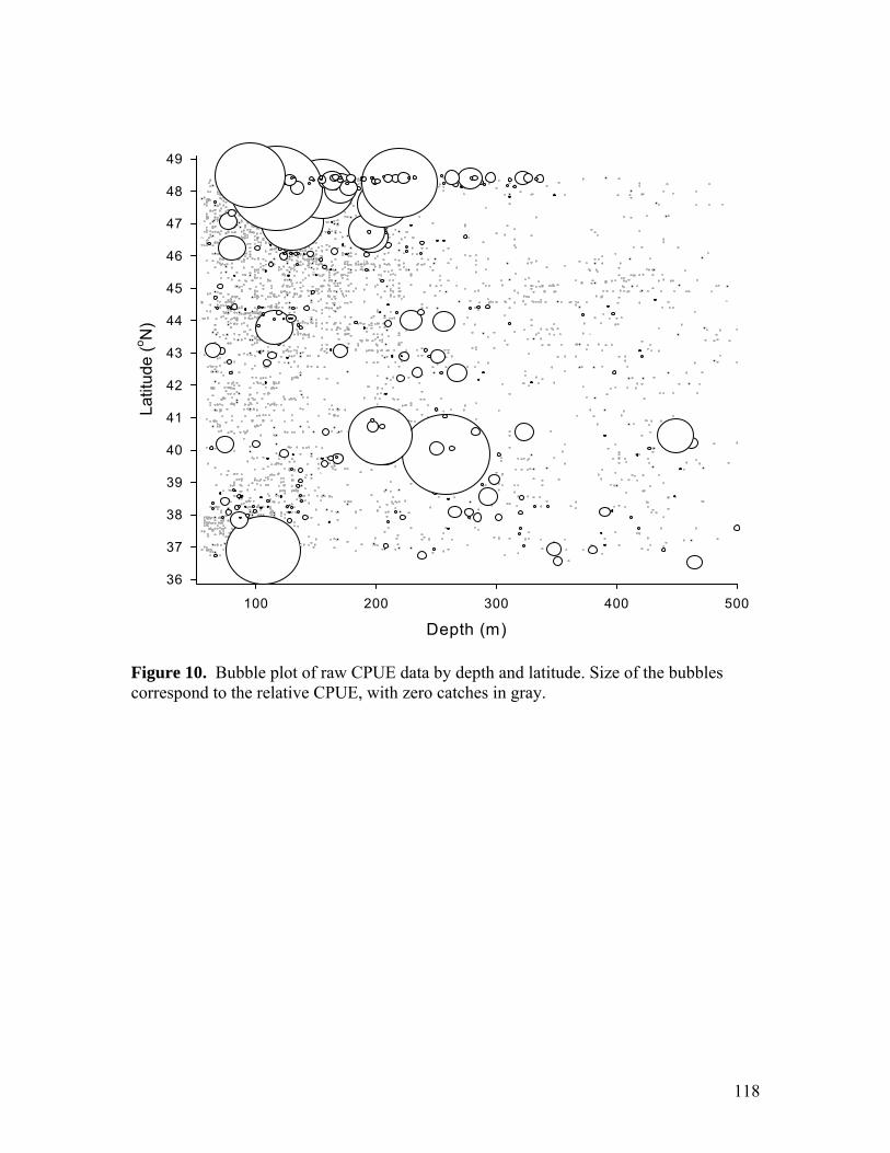
Depth (m)100 200 300 400 500

Latit

ude

(o N)

36

37

38

39

40

41

42

43

44

45

46

47

48

49

Figure 10. Bubble plot of raw CPUE data by depth and latitude. Size of the bubbles correspond to the relative CPUE, with zero catches in gray.

118

Appendix: Generalized linear model diagnostic graphs

In each of the following figures, individual models are identified by a letter scheme,

where:

A = slope

B = northern shelf and upper slope

C = southern shelf and upper slope

D = entire survey region with years grouped

119

A

B

Qua

ntile

Res

idua

ls

C Depth (m)

D Latitude (°N) Year

Figure 1. Quantile residuals against each explanatory variable for the binomial GLMs. Dotted line indicates the null pattern.

120

Figure 2. Standardized deviance residuals against each explanatory variable for the positive GLMs. Dotted line indicates the null pattern.

Year

A

B

Sta

ndar

dize

dD

evia

nce

Res

idua

ls

C Depth (m)

D Latitude (°N)

121

Qua

ntile

Res

idua

ls

D

C

B

A

Quantiles of Standard Normal Distribution

Figure 3. Quantile-quantile plots of the quantile residuals from the binomial GLMs, with a line fit through the first and third quantiles.

122

C

D

B

A

Sta

ndar

dize

d D

evia

nce

Res

idua

ls

Quantiles of Standard Normal Distribution

Figure 4. Quantile-quantile plots of the standardized deviance residuals from the binomial GLMs, with a line fit through the first and third quantiles.

123

Qua

ntile

Res

idua

ls

D

C

B

A

Fitted Values

Figure 5. Quantile residuals against fitted values for the binomial GLMs, with a Loess smoother (span = 2/3). Dotted line indicates the null pattern.

124

A

B S

tand

ardi

zed

Dev

ianc

eR

esid

uals

C

D Fitted Values

Figure 6. Standardized deviance residuals against fitted values for the positive GLMs, with a Loess smoother (span = 2/3). Dotted line indicates the null pattern.

125

Figure 7. Proportion of positive tows predicted by the binomial model against the proportion of positive tows observed. Cells with less than five observations were excluded from the analysis. Dotted line is a 1:1 reference.

Pre

dict

ed

Observed

A

0.0

0.2

0.4

0.6

0.8

1.0

0.0

0.2

0.4

0.6

0.8

1.0

B

0.0

0.2

0.4

0.6

0.8

1.0

C

0.0

0.2

0.4

0.6

0.8

1.0

D 0.0 0.2 0.4 0.6 0.8 1.0

126

Chapter 3

Assessment of the dorsal-fin spine for chimaeroid (Holocephali: Chimeriformes) age estimation

127

Introduction

Knowledge of fish age and growth characteristics is necessary for stock

assessment and development of successful management or conservation plans. Few

researchers have attempted to age chimaeroids (Calis et al. 2005; Freer and Griffiths

1993a; Johnson and Horton 1972; Moura et al. 2004; Sullivan 1977), and none have

convincingly validated their age estimates. Researchers have primarily used the dorsal-

fin spine as the ageing structure, because vertebral centra, commonly used to age other

chondrichthyans, are poorly calcified in holocephalans (personal observation, Johnson

and Horton 1972; Ridewood 1921). In Hydrolagus colliei, the number of transverse

ridges of vomerine tooth plates increases with body size, therefore has been proposed as a

promising ageing structure (Johnson and Horton 1972; Simmons and Laurie 1972).

These ridges may be ephemeral, however, as they are likely formed by a combination of

deposition and erosion of the ever-growing tooth plates (Didier et al. 1994), a process

which may be extremely rapid (Ward and Grande 1991). These ridges may be serially

replaced, leading to underestimation of lifetime growth and age (Didier and Rosenberger

2002). Modal analyses of length-frequency distribution, and eye lens diameter and

weight may be used to determine the age structure of chimaeroids (Francis 1997; Francis

and Maolagáin unpublished), but are likely only useful for verification of ageing from a

hard part composed of calcium phosphate or dentine (Cailliet and Goldman 2004).

The dorsal-fin spine may have been derived from modifications of individual

(Goodrich 1909) or multiple scales (Patterson 1965), but its derivation remains

controversial (Maisey 1979). Halstead and Bunker (1952) indicated that the spine stem is

composed of vasodentine, and the interior is a pulp cavity occupied by a cartilaginous rod

128

enveloped by a layer of areolar connective tissue. Halstead and Bunker (1952) described

the spine as having a thin outer layer of integument, consisting of an outer avascular

epidermis of squamous epithelium, and an inner vascularized dermis of fibrous

connective tissue. An enamel layer, which is present in dorsal-fin spines of squaloid

sharks, has not been identified in the chimaeroid dorsal-fin spine (Goodrich 1909;

Halstead and Bunker 1952).

Based on the growth of elasmobranch dorsal-fin spines, researchers have assumed

the chimaeroid spine grows primarily by secretions of cells in the spine lumen that

deposit dentine on the inner surface of the spine (Holden and Meadows 1962). This type

of growth would create conical growth zones stacked on top of one another, each new

growth zone displacing the previous growth zones distally. Chimaeroid dorsal-fin spines

have only one inner and outer layer of dentine (Calis et al. 2005), and there is debate

among authors whether elasmobranch dorsal-fin spines have two or three dentine layers

(review in Clarke and Irvine 2006). Early squaloid researchers interpreted opaque and

translucent band pairs within the inner layer of dorsal-fin spines as dentine growth

increments deposited with consistent, annual periodicity (Kaganovskaia 1933), but this

was only validated for Squalus acanthias (Campana et al. 2006; McFarlane and Beamish

1987; Tucker 1985).

I test the hypothesis that the dorsal-fin spine of H. colliei is a reliable structure for

age estimation. To aid interpretation of spine growth, the internal structure of the spine

was compared with hard parts used for age determination of other fishes. Knowledge of

H. colliei age and growth dynamics is necessary to determine its vulnerability to fishing

129

mortality, currently applied as discard mortality from the commercial groundfisheries of

the eastern North Pacific.


Age and Growth Determination

The dorsal-fin spine was the primary structure evaluated for age estimation of H.

colliei. Dorsal-fin spines were excised from each individual and stored frozen.

Transverse (perpendicular to axis of spine) sectioning of the spine has produced the best

results for ageing in other chimaeroids (Calis et al. 2005; Francis and Maolagáin

unpublished; Freer and Griffiths 1993a; Sullivan 1977), however, I also attempted

longitudinal sectioning to visualize the entire zone of dentine deposition. For a subset of

spines, transverse and longitudinal sections were collected from a single spine for direct

comparison of growth bands. Dorsal-fin spine terminology follows Clarke and Irvine

(2006).

To locate the appropriate region on the spine to extract transverse sections,

morphometric measurements of dried dorsal-fin spines were recorded to the nearest mm

(after Calis et al. 2005). Not all measurements were consistent, however, as many

individuals had obvious wear of the spine tip. To address this problem, past researchers

created a correction factor, using the linear relationship of spine width at fixed positions

on the longitudinal axis of unworn spines (Sullivan 1977). After correcting spine lengths,

and sectioning and analyzing a representative sample of spines for growth increments, the

best sectioning position for ageing was determined by the distance from the actual or

theoretical unworn spine tip. In this study, the validity of using lateral spine width as a

130

proxy for the distance from the spine tip was tested with ANCOVA, using width as the

dependent variable, individual as a random independent factor, and distance from the

spine tip as a covariate. In the first phase of this sampling, width was measured

microscopically at multiple fixed distances from the spine tip (following Sullivan 1977),

then later at multiple random distances. These two datasets produced the same results

when tested separately, so data were combined for the final test. In the early stages of

experimentation, spines were sectioned throughout the ageable region to establish the

lateral spine width and distance from spine tip that contained a cross section of all dentine

deposits to prevent underestimation of age. At least six sections were taken from each

specimen, with section thickness varying from 0.1 to 0.6 mm, selected to include the

optimal range in previous studies (Calis et al. 2005; Francis and Maolagáin unpublished;

Freer and Griffiths 1993a).

Before sectioning, spines were embedded in a polyester casting resin, which was

allowed to harden for 24 h. Sections were cut using a Buehler Isomet low-speed saw

with diamond-impregnated blade. Subsequently sections were polished with 1200- grit

sandpaper to remove saw scratches and create a smooth surface. Sections were mounted

on a microscope slide for enumeration of growth bands. Transmitted, reflected, and

polarized light were used in microscopic analysis of the spine to determine the optimal

lighting method for discerning growth bands. Several dorsal-fin spines were embedded,

stained with Harris hematoxylin, and sectioned on a microtome for histological analysis

using the methods of Natanson et al. (2007). To determine whether growth bands were

indicative of somatic growth, band counts were plotted against snout-vent length (SVL)

and total body mass.

131

Hard parts used in ageing must grow in proportion to body size to be considered

an adequate ageing structure. Therefore, SVL was compared with several morphometric

measurements of the dorsal-fin spine to test the assumption of a positive relationship

between body size and dorsal-fin spine size. Each relationship was modelled with the

linear or non-linear regression function that produced the best fit.

The hypothesized annual periodicity of growth band deposition was tested with

direct validation by chemical marking with oxytetracycline (OTC). Three captive ratfish,

held at the Vancouver Aquarium, were injected with a 25 mg kg-1 body weight dose

(Holden and Vince 1973) of OTC. After one year of growth, dorsal-fin spines were

removed, sectioned, and viewed under reflected ultraviolet light. Care was taken to

minimize the intensity and duration of sample exposure to ambient light to avoid

degradation of the fluorescent properties of OTC.

Computed Tomography

Precise and accurate age estimation was challenging because of the lack of

information about spine structure and development. The traditional technique of

microscopic examination of thin-sectioned spines provides limited inference, as among-

individual variation in the distribution of growth increments may prevent precise age

estimation and validation. Radiological resources, therefore, were used to elucidate the

physiological parameters of interest. Simple x-ray technology was insufficient, however,

because of the small focal size necessary to resolve features on the scale of tens of

microns. Analyses also were hampered by attempts to visualize a 3-dimensional object in

a 2-dimensional projection. These problems were addressed by using computed

132

tomography to visualize the dorsal-fin spine with 3-dimensional imaging. Computed

tomography (CT) is a radiological imaging technique that is analogous to a 3-dimensional

x-ray. This study used micro-computed tomography (µCT), which is the same method as

CT, but with greatly decreased voxel size (increased resolution). All scans were 16-bit

gray scale, with 6 micron isotropic voxel size. This technique is the state-of-the-art in

high-resolution, 3-dimensional imaging of dense structures, yet this study is the first to

use µCT for age determination.

For comparative purposes, µCT scans also were performed on ageing structures

commonly used in other organisms. Structures included the dorsal-fin spine and vertebra

of spiny dogfish (Squalus acanthias), vertebra and caudal thorn of roughtail skate

(Bathyraja trachura), and otolith of Patagonian toothfish (Dissostichus eleginoides). The

vertebra and neural arch of H. colliei also were scanned to determine their potential as

ageing structures.

Results

Growth

Longitudinal sectioning was not successful in elucidating all growth increments.

Longitudinal bands were only observed in two out of six spines, and only once were the

band counts similar between longitudinal and transverse sections. Histological methods

were not successful in producing sections with visible growth bands.

The length from base to tip (total spine length or TSL) of unworn dorsal-fin

spines increased linearly with SVL (t = 34.041, df = 19, p < 0.001, R2 = 0.984; Fig. 1A).

The distance from spine tip to the apex of the pulp cavity (apex spine length or ASL)

133

increased linearly with SVL (t = 7.817, df = 19, p < 0.001, R2 = 0.760; Fig. 1B).

Similarly, the lateral spine width at the apex of the pulp cavity (apex pulp cavity

diameter, or APC) increased linearly with SVL (t = 8.082, df = 19, p < 0.001, R2 = 0.772;

Fig. 1C).

Lateral spine width along the longitudinal axis of the spine was not a consistent

indicator of distance from the spine tip. The relationship between distance from spine tip

and spine width varied among individuals (ANCOVA: factor = spine length*individual,

F = 2.807; df = 27; p = 0.001; Fig. 2). Therefore, it is not possible to assure that

transverse sections are collected at the same position among individuals, relative to

growth zones.

Transverse sections viewed with incandescent transmitted light revealed much

about the internal structure of the spine’s dentine portions. The anterior dentine portion

was composed of trabecular dentine (Fig. 3A), overlying the outer and inner concentric

laminar dentine layers of the stem (Fig. 3B). The orientation of the canaliculi (the

network of dentritic vessels within the dentine) indicated the inner dentine layer was

deposited centripetally, and the outer dentine layer was deposited centrifugally. In the

anterior dentine portion, dentine is deposited centripetally around each vascular canal.

Standard incandescent transmitted and reflected light failed to reveal clear growth

increments in transverse sections. However, when viewed with transmitted light

combined with a polarizing filter, zones of dark and light alternating bands were observed

within the inner dentine layer (Fig. 4). These bands were most apparent in 0.4 mm thick

sections. The greatest number of bands was found in sections 8.8 to 9.4 mm from the

spine tip, near the apex of the pulp cavity.

134

The number of band pairs observed in the inner dentine layer was not a good

predictor of body size. There was a trend indicating that the number of bands increased

with SVL and total mass, but there was great variability (Fig. 5). No attempts were made

to model the relationship because of the small sample size and the great inherent

uncertainty.

Validation attempts by injection with OTC were inconclusive. The substance was

not incorporated into the dorsal-fin spine dentine. Irregular patters of fluorescence were

observed in the soft tissues of the spine exterior and vascular canals, but they cannot be

attributed to OTC injection.

Physiology of Hard Parts

As expected, mineral density gradients, potentially representing discrete growth

zones, were observed in the hard parts of elasmobranch and teleost specimens. Such

density gradients were observed in the second dorsal-fin spine (Fig. 6A) and vertebra

(Fig. 6B) of S. acanthias. Scans of the spine revealed three large bands, representing the

inner and outer dentine layers, separated by the trunk primordium (Maisey 1979). The

enamel and dentine of the cap was distinguishable on the posterior-lateral edge.

Mineral density gradients were observed in the vertebra (Fig. 7A) and caudal

thorns (Fig. 7B) of B. trachura. Micro-CT scans from the otolith of D. eleginoides also

revealed well-defined density gradients (Fig. 8). These gradients were distributed in

patterns consistent with their interpretation as growth zones from observations using light

microscopy.

135

Mineral density gradients were not observed in the H. colliei dorsal-fin spine (Fig.

9). Numerous vascular canals were observed on the anterior and posterior edges of the

spine. The canals connected the spine lumen to the spine exterior. Canals were present

at irregular intervals along the majority of the spine’s length, but were more concentrated

toward the tip.

The vertebra and neural arch (Fig. 10) of H. colliei were poorly calcified.

Vertebral centra were entirely absent from two of the three μCT scans, and visible only as

translucent streaks in the other. The neural arch had very thin walls, with greater density

in the interior of the wall than the exterior.

Discussion

Growth

The vertebral centra and neural arch of H. colliei were poorly calcified, therefore,

likely useless as structures for age determination. Encouraging results had been obtained

from the use of neural arches for aging the bluntnose sixgill shark, Hexanchus griseus

(McFarlane et al. 2002), but this is not the case for H. colliei. The dorsal-fin spine does

show some promise as a structure for ageing, as it grows continuously with body size.

TSL, ASL, and APC increased linearly with SVL, providing clear interpretation of the

relationship between spine growth and body size. The fit of TSL on SVL was

particularly good, and provides support for the use of dorsal-fin spines for ageing.

Variation among individuals in the relationship between spine width at length from the

spine tip, however, indicated that the technique of transverse sectioning may confound

age determination.

136

Previous researchers hypothesized the optimal point of transverse sectioning was

a set distance from the spine tip. To test this hypothesis, researchers measured lateral

spine width at varying distances from the spine tip for many individuals. With

individuals pooled, spine width was regressed on spine length, typically with a fairly

good fit (e.g. Sullivan 1977). Based on that evidence, spine width was used to determine

appropriate distance from tip for transverse sectioning. An ANCOVA, however,

indicated that there was significant among-individual variation in the length to width

relationship. Width, therefore, is not a good indicator of the point where all growth zones

can be viewed. This means that it is not possible to section at the same point on every

spine, relative to the growth zones. Thus, this type of spine growth, observed with this

technique of sectioning, precludes the use of validation tools such as marginal increment

analysis and edge analysis (e.g. Guillart-Furio 1998). These complications further

impede accurate and precise age estimation using the dorsal-fin spine.

The greatest band pair counts were in transverse sections near the apex of the pulp

cavity. This point, however, can be as far as 16 mm from the spine tip, whereas the length

of the entire spine can be as short as 13 mm. In older individuals, there may be no

transverse plane at which all growth zones overlap. This would lead to underestimation

of age. Underestimation of ages using internal growth bands also occurred in the ageing

of squaloid dorsal-fin spines, perhaps because of lack of formation of additional growth

zones in older individuals (Irvine et al. 2006a; Irvine et al. 2006b), or because growth

zones were indistinguishable with advanced age (Irvine et al. 2006a). The results of this

study indicate age estimates using the dorsal-fin spine of chimaeroids were prone to

imprecision, or even bias, based on the region of transverse section.

137

Age validation attempts with laboratory grow-outs of OTC-injected H. colliei

failed. The OTC was not incorporated internally, similar to observations of the chain

dogfish, Scyliorhinus retifer (Lisa Natanson, NOAA Fisheries, Southeast Fisheries

Science Center, pers. comm.). The fluorescence observed in the soft tissues of the spine

could not have been caused by OTC, as it becomes absent from circulation within four

months of injection in elasmobranchs (Tanaka 1990). The fluorescence in the soft tissues

must be caused by a naturally-occurring substance.

Physiology of Hard Parts

Vascular canals were observed in the anterior and posterior edges of the H. colliei

dorsal-fin spine, connecting the spine lumen with the spine exterior. This indicates that

the vascular system of the chimaeroid dorsal-fin spine functions similarly to

elasmobranch dorsal-fin spines sensu Maisey (1979). Arterial blood is supplied to the

spine by small blood vessels leading distally within the loose connective tissue of the

spine lumen. These vessels exit the spine lumen anteriorly and posteriorly through

vascular canals that penetrate the stem. Veins in the anterior dentine portion and its

associated dermis lead proximally to the spine base.

The dorsal-fin spine is not composed of vasodentine as proposed by Halstead and

Bunker (1952). Instead, the inner, and perhaps outer, dentine layers are composed of

orthodentine (Patterson 1965; Schaeffer 1977), as in elasmobranch dorsal-fin spines

(Maisey 1979). The anterior dentine portion, and perhaps the posterior-lateral dentine

portions, are likely composed of osteodentine (Patterson 1965), or a similar substance of

unknown definition (Maisey 1979). This composition and orientation of growth surfaces

138

confirms that the bands observed in the inner dentine layer may indeed be indicative of

incremental growth. However, the periodicity with which these zones are formed may

not be consistent, which would explain the poor relationship between band pair number

and body size. This phenomenon of inconsistent periodicity of band pair formation also

has been observed in Pacific angel shark (Squatina californica) vertebrae (Cailliet et al.

1983; Natanson and Cailliet 1990).

Growth may not occur on all depositional surfaces of the spine throughout

ontogeny. Halstead and Bunker (1952) observed odontoblasts (the cells which produce

dentine) on the inner surface of the stem in spines from young individuals only,

indicating that dentine deposition in the inner dentine layer may cease once a particular

age or size is achieved. This observation may have been confounded by taking transverse

sections too close to the spine base, yet it still calls into question the utility of the inner

dentine layer as a complete growth record.

The lack of density gradients observed in H. colliei dorsal-fin spines is likely a

real phenomenon, not an artifact of CT scanning (e.g. beam hardening). The alternating

bands observed with polarized light may be transitions between zones of the spine with

differing proteinaceous fiber orientation, instead of many extremely thin layers of dentine

deposited in bands of alternating thickness (e.g. calcium deposition in teleost otoliths or

elasmobranch vertebrae). The mere presence of varying fiber orientation, opposed to

mineral density gradients, decreases the likelihood that the bands observed represent a

record of growth with consistent periodicity. This provides some tentative evidence that

H. colliei may have aseasonal growth.

139

Conclusions

Future research is necessary before chimaeroid dorsal-fin spines can be used for

age estimation. Subsequent studies should continue attempting description of spine

structure and growth using alternative techniques, including histology. Validation is

needed to evaluate the accuracy of past and future chimaeroid age estimates. Alternative

validation methods will need to be employed, as this study refutes the applicability of

marginal increment analysis, edge analysis, and chemical marking with OTC. Until the

periodicity of growth is validated, the hypothesis of aseasonal growth remains plausible

and it should not be assumed that age is quantifiable by standard techniques.

140

Literature Cited

Cailliet GM, Goldman KJ (2004) Age determination and validation in chondrichthyan

fishes. In: Carrier JC, Musick JA, Heithaus MR (eds) Biology of sharks and their

relatives. CRC Press, Boca Raton, FL, pp 399-448

Cailliet GM, Martin LK, Kusher D, Wolf P, Welden BA (1983) Techniques for

enhancing vertebral bands in age estimation of California elasmobranchs. In:

Prince E, Pulos L (eds) Proceedings of the international workshop on age

determination of oceanic pelagic fishes: tunas, billfishes, and sharks, pp 157-165

Calis E, Jackson EH, Nolan CP, Jeal F (2005) Preliminary age and growth estimates of

the rabbitfish, Chimaera monstrosa, with implications for future resource

management. e-Journal of Northwest Atlantic Fisheries Science 35

Campana SE, Jones C, McFarlane GA, Myklevoll S (2006) Bomb dating and age

validation using the spines of spiny dogfish (Squalus acanthias). Environmental

Biology of Fishes 77

Clarke MW, Irvine SB (2006) Terminology for the ageing of chondrichthyan fish using

dorsal-fin spines. Environmental Biology of Fishes 77: 273-277

Didier DA, Rosenberger LJ (2002) The spotted ratfish, Hydrolagus colliei: notes on its

biology with a redescription of the species (Holocephali: Chimaeridae). California

Fish and Came 88: 112-125

Didier DA, Stahl BJ, Zangerl R (1994) Development and growth of compound tooth

plates in Callorhinchus milii (Chondrichthyes, Holocephali). Journal of

Morphology 222: 73-89

141

Francis MP (1997) Spatial and temporal variation in the growth rate of elephantfish

(Callorhinchus milii). New Zealand Journal of Marine and Freshwater Research

31: 9-23

Francis MP, Maolagáin CÓ (unpublished) Development of ageing techniques for dark

ghost shark (Hydrolagus novaezelandiae). National Institute of Water and

Atmospheric Research

Freer DWL, Griffiths CL (1993) Estimation of age and growth in the St. Joseph

Callorhinchus capensis (Dumeril). South African Journal of Marine Science 13:

75-81

Goodrich ES (1909) A treatise on zoology. Adam and Charles Black, London

Guillart-Furio J (1998) Contribution to the knowledge of the biology and taxonomy of

the deepsea shark, Centrophorus granulosus (Bloch and Schneider, 1801)

(Elasmobranchii, Squalidae) in the Balearic Sea (western Mediterranean). Ph.D.

Thesis

Halstead BW, Bunker NC (1952) The venom apparatus of the ratfish, Hydrolagus colliei.

Copeia 3: 128-138

Holden MJ, Meadows PS (1962) The structure of the spine of the spur dogfish (Squalus

acanthias L.) and its use for age determination. Journal of the Marine Biological


Holden MJ, Vince MR (1973) Age validation studies on the centra of Raja clavata using

tetracycline. Journal du Conseil 35: 13-17

Irvine SB, Stevens JD, Laurenson LJB (2006a) Comparing external and internal dorsal-

spine bands to interpret the age and growth of the giant lantern shark, Etmopterus

142

baxteri (Squaliformes: Etmopteridae). Environmental Biology of Fishes 77: 253-

264

Irvine SB, Stevens JD, Laurenson LJB (2006b) Surface bands on deepwater squalid

dorsal-fin spines: an alternative method for ageing the golden dogfish

Centroselachus crepidater. Canadian Journal of Fisheries and Aquatic Sciences

63: 617-627

Johnson AG, Horton HF (1972) Length-weight relationship, food habits, parasites, and

sex and age determination of the ratfish, Hydrolagus colliei (Lay and Bennett).


Kaganovskaia S (1933) A method of determining the age and the composition of the

catches of the spiny dogfish (Squalus acanthias L.). Bulletin Far-East Br Acad Sci

USSR 1(3):5-6 (translated from Russian by W.E. Ricker). Fisheries Research

Board of Canada, Translation Series 281(1):5-6

Maisey JG (1979) Finspine morphogenesis in squalid and heterodontid sharks.

Zoological Journal of the Linnean Society 66: 161-183

McFarlane GA, Beamish RJ (1987) Validation of the dorsal spine method of age

determination for spiny dogfish. The Iowa State University Press, Iowa

McFarlane GA, King JR, Saunders MW (2002) Preliminary study on the use of neural

arches in the age determination of bluntnose sixgill sharks (Hexanchus griseus).


Moura T, Figueiredo I, Machado PB, Gordo LS (2004) Growth pattern and reproductive

strategy of the holocephalan Chimaera monstrosa along the Portuguese

143

continental slope. Journal of the Marine Biological Association of the United

Kingdom 84: 801-804

Natanson LJ, Cailliet GM (1990) Vertebral growth zone deposition in Pacific angel

sharks. Copeia 1990: 1133-1145

Natanson LJ, Sulikowski JA, Kneebone JR, Tsang PC (2007) Age and growth estimates

for the smooth skate, Malacoraja senta, in the Gulf of Maine. Environmental

Biology of Fishes

Patterson C (1965) The phylogeny of the chimaeroids. Philosophical Transactions of the

Royal Society of London, Series B 249: 101-219

Ridewood WG (1921) On the calcification of the vertebral centra in sharks and rays.

Philosophical Transactions of the Royal Society of London, Series B 210: 311-

407

Schaeffer B (1977) The dermal skeleton in fishes. In: Andrews SM, Miles RS, Walker

AD (eds) Problems in vertebrate evolution. Academic Press, Inc., New York, NY,

pp 25-52

Simmons JE, Laurie JS (1972) A study of Gyrocotyle in the San Juan Archipelago, Puget

Sound, U.S.A., with observations on the host, Hydrolagus colliei (Lay and

Bennett). International Journal for Parasitology 2: 59-77

Sullivan KJ (1977) Age and growth of the elephant fish Callorhinchus milii

(Elasmobranchii: Callorhynchidae). New Zealand Journal of Marine and

Freshwater Research 11: 743-755

Tanaka S (1990) Age and growth studies on the calcified structures of newborn sharks in

laboratory aquaria using tetracycline. In: Pratt Jr HL, Gruber SH, Taniuchi T (eds)

144

Elasmobranchs as living resources: advances in the biology, ecology, systematics,

and the status of the fisheries. NOAA Technical Report pp 189-202

Tucker R (1985) Age validation studies on the spines of the spurdog (Squalus acanthias)

using tetracycline. Journal of the Marine Biological Association of the U.K. 35:

641-651

Ward DJ, Grande L (1991) Chimaeroid fish remains from Seymour Island, Antarctic

Peninsula. Antarctic Science 3: 323-330

145

0 50 100 150 200 250 300

Tota

l Spi

ne L

engt

h (m

m)

0

20

40

60

80

100

120

0 50 100 150 200 250 300

Spin

e Ti

p to

Ape

x of

Pul

p C

avity

(mm

)

0

2

4

6

8

10

12

14

16

18

20

22


0 50 100 150 200 250 300

Late

ral S

pine

Wid

th a

t Ape

x of

Pul

p C

avity

(mm

)

0.4

0.6

0.8

1.0

1.2

1.4

1.6

1.8

2.0

2.2

A

B

C

Figure 1. Comparison of snout-vent length to (A) total dorsal-fin spine length, (B) distance between the dorsal-fin spine tip and the apex of the pulp cavity, and (C) dorsal-fin spine width at the apex of the pulp cavity.

146

Distance from Spine Tip (mm)

0 5 10 15 20 25

Late

ral S

pine

Wid

th (m

m)

0.2

0.4

0.6

0.8

1.0

1.2

1.4

1.6

1.8

2.0

2.2

Figure 2. Comparison of distance from dorsal-fin spine tip and spine width among individuals (n = 28). Lines represent linear regressions for each individual.

147

A

B

Figure 3. Photomicrograph of a transversely sectioned dorsal-fin spine (A) anterior dentine portion, and (B) posterior face, viewed with transmitted light. SL = spine lumen; IL = inner dentine layer; OL = outer dentine layer. Scale = 0.5 mm.

148

Figure 4. Photomicrograph of a transversely sectioned dorsal-fin spine viewed with polarized, transmitted light. Scale = 0.5 mm.

149

2 4 6 8 10 12

Sno

ut-V

ent L

engt

h (m

m)

100

120

140

160

180

200

220

240

260

280

Band Pairs

2 4 6 8 10 12

Tota

l Wei

ght (

kg)

0.0

0.2

0.4

0.6

0.8

1.0

1.2

1.4

1.6

A

B

Figure 5. Comparison of the number of dorsal-fin spine band pairs to (A) snout-vent length, and (B) total mass for females (n = 16).

150

A

B

Figure 6. µCT image of the (A) transverse plane of a second dorsal fin spine, and (B) the longitudinal plane of a vertebra from S. acanthias. Arrows indicate density gradients that may represent distinct growth zones. Scale = 0.5 mm.

151

B

A

Figure 7. µCT image of the (A) transverse plane of a vertebra, and (B) the longitudinal plane of a caudal thorn (just anterior to the thorn tip) from B. trachura. Arrows indicate density gradients that may represent distinct growth zones. Scale = 0.5 mm.

152

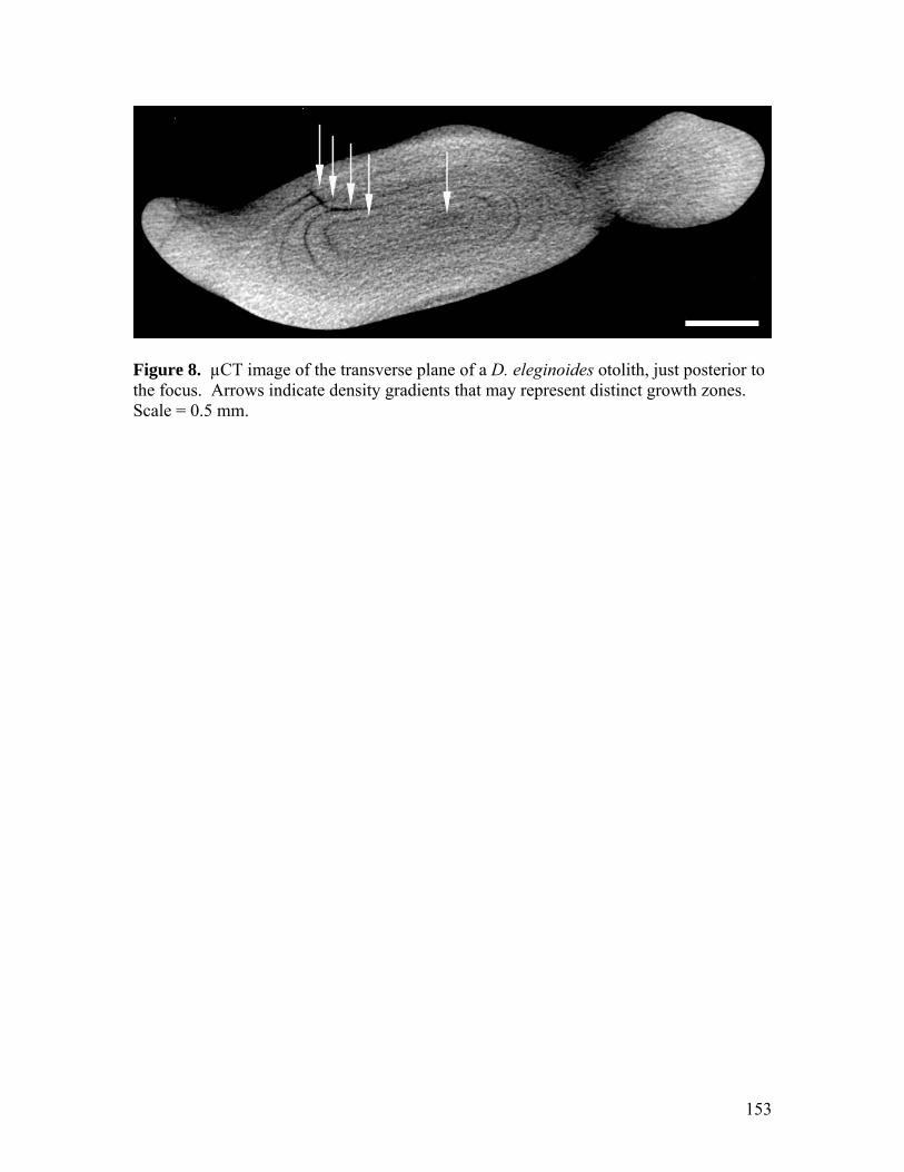
Figure 8. µCT image of the transverse plane of a D. eleginoides otolith, just posterior to the focus. Arrows indicate density gradients that may represent distinct growth zones. Scale = 0.5 mm.

153

B C

A A

Figure 9. µCT images of the H. colliei dorsal-fin spine, in the longitudinal (dorso-ventral) plane (A), and in the transverse plane, depicting dentine canals leading to the posterior (B) and anterior (C) spine exterior. Scale = 0.5 mm.

154

B

C

A

Figure 10. µCT images of the H. colliei neural arch and vertebrae, from the transverse plane (A), and the longitudinal plane (B and C). Scale = 0.5 mm.

155

LIFE HISTORY, ABUNDANCE, AND DISTRIBUTION OF THE SPOTTED

Documents

Transcript of LIFE HISTORY, ABUNDANCE, AND DISTRIBUTION OF THE SPOTTED