Life histories: real and synthetic

Frans Willekens

MPIDR, Rostock

September 2014

2

Abstract

Life history data are generally incomplete. Respondents enter observation late (left

truncation) or leave early (right censoring). In survival analysis, these limitations are

considered in the estimation of hazard rates. Rates are estimated from data on

different respondents with different observation periods (observation windows). In

multistate modeling, transition rates also integrate information on different

individuals.

By combining data from different but similar individuals, life histories can be

modeled. The life history that results is a synthetic life history. It is not observed and

it does not tell anything about a particular individual. It tells something about the

population the individual is part of. A synthetic biography summarizes information on

several individuals. The collective experience is summarized in transition rates. The

individual is a fictitious individual, referred to as virtual individual or statistical

individual (Courgeau, 2012). A population of virtual individuals is a virtual

population. The life history of such an individual is not directly observed but is an

outcome of a probability model, the parameters of which are estimated from empirical

data. Life histories are generated from models using microsimulation in continuous

time.

Several life course indicators may be derived from transition rates. They include

probabilities of significant transitions, probabilities of having reached particular

stages in life, expected durations of stages of life, and expected ages at significant

transitions.

The methods are illustrated using data from the German Life History Survey (GLHS).

It is a subsample also used by Blossfeld and Rohwer (2002) in their book Techniques

of Event History Modeling. In the paper, references are made to R packages for

multistate modelling and analysis, in particular mvna, etm, msm, mstate, ELECT and

Biograph.

3

Life histories: real and synthetic

1. Introduction

Life history data are generally incomplete. Usually, they do not cover for each

individual in the study the entire life span or the life segment of interest. If data are

collected retrospectively, observation ends at interview date and no information is

available on events and experiences after the date. Data collected prospectively are

incomplete because events and other experiences are recorded during a limited period

of time only. To deal with data limitations, models are introduced. The model that is

considered in this chapter describes life histories. The model is based on the premise

that life histories are realizations of a continuous-time Markov process. A Markov

process is a stochastic process that describes a system with multiple states and

transitions between the states. The time at which a transition occurs is random but the

distribution of the time to transition is known. In the continuous-time Markov

process, the transition time has an exponential distribution. The rate of transition out

of the current state (exit rate) is the parameter of the exponential distribution. It

depends on the current state only and is independent of the history of the stochastic

process. In a system with multiple states, an individual who leaves the current state

may enter one of several states. In competing risks models, states in the state space

are viewed as competing destinations and transition rates are destination-specific. The

Markov process is a first-order process: the destination state depends on the current

state only and is independent of states occupied previously.

The Markov model predicts1 the probability that an individual of a given age occupies

a given state. The Markov model may also be used to predict the number of

transitions during a given interval and the number of times an individual occupies a

given state. The stochastic process that describes the transition counts or the state

occupancy counts is a Markov counting process (see below). It belongs to the class of

counting processes. The most elementary counting process is the Poisson process. It is

a stochastic process that counts the number of transitions without considering origin

and destination states. In a Poisson process, the time between two consecutive

transitions has an exponential distribution.

The parameters of the Markov model are estimated from data. By pooling data on

different but similar individuals, models can be estimated that describe the entire life

histories. The life history that is based on pooled data is a synthetic life history. It is a

virtual life history; it is not observed. It does not say anything about a specific

individual in a sample but tells something about the sample the individual is part of. A

synthetic biography summarizes information on several individuals. It is the life

course that would result if an individual lives a life prescribed by the collective

experience of similar individuals under observation. The collective experience is

summarized in transition rates. These rates play a key role in generating synthetic

biographies. Transition rates are estimated from life history data and used to generate

synthetic biographies. Maximum likelihood estimates of transition rates are used to

1 Prediction is used in the statistical meaning. Prediction is a statement about an outcome. A model is

often used to predict an outcome, e.g. an event that occurs in a population or that is experienced by an

individual in a population. The parameter(s) of the model are estimated from observations on a

selection of individuals. Prediction is part of statistical inference. It should not be confused with

forecasting.

4

generate expected life histories and expected values of life history indicators.

Individual life histories are distributed randomly around an expected life path.

Microsimulation is used to generate individual life histories from empirical transition

rates.

In life history analysis and life history modelling, age is the main time scale. Age is a

proxy for stage of life. Other useful time scales are calendar time and time since a

reference event. Birth, marriage, labour market entry, and entry into observation are

examples of reference events. The standard approach in survival analysis is to use

time since the baseline survey or (first) entry into the study (time-on-study). Time-on-

study has no explanatory power, which is acceptable if time dependence of a

transition rate is not of interest, such as in the Cox model with free baseline hazard.

Korn et al. (1997) argue that time-on-study is not appropriate for predicting transition

rates. They recommend age as the time scale (see also Pencina et al., 2007 and Meira-

Machado et al., 2009). Rates of transition between states generally vary with age. The

Markov process that accommodates changing rates is the time-inhomogeneous

Markov process. The model of that process is discussed in this chapter.

To characterize life histories, a set of indicators is usually used, including state

occupancies at consecutive ages, durations of stages of life, and ages at significant

transitions. The indicators are sometimes combined in a table, known as the multistate

life table. The multistate life table originated in demography (Rogers, 1975), but it is

currently used across disciplines. The model that produces the values of the indicators

summarized in the multistate life table is the Markov process model.

Two examples may clarify the concept of synthetic biography. The first relates to the

length of life and the second to marriage and fertility.

a. Suppose we are interested in the life expectancy of a 60-year old. The

empirical evidence consists of a 10-year follow-up of 1000 individuals aged

60 and over. At the beginning of the observation period, some individuals are

relatively young (60 years, say) while others are already old (over 90, say).

During the observation period of 10 years, some individuals die. The oldest

old are more likely to die than other individuals under observation. To

determine the expected remaining lifetime for a 60-year old, one could

calculate the mean age at death of those who die during the observation

interval. The observed mean age at death provides a wrong answer, however.

It depends on the age composition of the population under observation. If the

group under observation consists of many old persons, the mean age at death

will be higher than for a group that consists mainly of persons in their sixties

and seventies. To remove the effect of the age composition, death rates are

calculated by age. The distribution of ages at death is obtained by applying a

piecewise exponential survival model, with parameters the age-specific

mortality rates. The expected age at death is 60 plus the expected remaining

lifetime or life expectancy. The life expectancy of a 60-year old is the number

of years that the individual may expect to live if at each age over 60 he

experiences the age-specific mortality rate estimated during the 10-year

follow-up of 1000 individuals. At young ages, he experiences the mortality

rates of individuals who were 60 recently. At older ages the mortality rates are

from old persons who turned 60 many years ago. The life expectancy is

adequate if the age-specific mortality rates do not vary in time.

5

b. The second illustration considers marriage and fertility. Suppose we want to

know at what age women start marriage and at what duration of marriage they

have their first child. It is not possible to follow all women until they have

their first child since some will remain childless. Suppose the data are from a

5-year follow-up survey of girls and women aged 15 to 35 at the onset of

observation. At the end they are 20 to 40. During the follow-up, the age at

marriage and the age at birth of the first child are recorded. At the start of

observation, some individuals are already married. Other individuals remain

unmarried during the entire period of observation. They may marry after

observation is ended or they may not marry at all. To determine the age at

marriage and the duration of marriage at time of birth of the first child,

marriage and childbirth are described by a continuous-time Markov process

with transition rates the empirical marriage rates and marital first birth rates.

The model describes the marriage and first birth behaviour of hypothetical and

identical individuals of age 15 assuming that at consecutive ages they

experience the empirical rates of marriage and first birth. Transition rates may

depend on covariates and other factors.

This chapter consists of two parts. The first part (Section 2) is devoted to the

estimation of transition rates from data. The second part (Sections 3 to 5) focuses on

synthetic biographies. Section 3 shows how transition probabilities and state

occupation probabilities are computed from transition rates. The computation of

expected occupation times is covered in Section 4. The generation of synthetic life

histories is discussed in Section 5. Section 6 is the conclusion.

The methods presented in this chapter are illustrated using employment data from a

subsample of 201 respondents of the German Life History Survey (GLHS) (see

Chapter 1). Two states are distinguished: employed (Job) and not employed (Nojob).

Transitions are from employed to not employed (JN) and from not employed to

employed (NJ). Dates of transition are given in months; it is assumed that transitions

occur at the beginning of a month. In the chapter, references are made to R packages

for multistate modeling and analysis, in particular mvna (Allignol, 2012; Allignol et

al., 2008), etm (Allignol, 2013; Allignol et al., 2011), msm (Jackson, 2011, 2013),

mstate (Putter et al., 2012; de Wreede et al., 2010, 2011), dynpred (Putter, 2011),

ELECT (van den Hout, 2013) and Biograph (Willekens, 2013).

2. Transition rates

Transition rates are the parameters of the Markov process that underlies the multistate

life history model. In this section, two broad approaches for estimating transition rates

are covered. Age, which is the time scale, is treated as a continuous variable.

Transitions may occur at any age. Transition rates are estimated by relating transitions

to exposures. In the first approach, transition rates may vary freely with age. The age

profile is not constrained in any way. In the second approach, transition rates are

restricted to follow an age profile described by a parametric model. The first approach

is non-parametric; the second is parametric. The two approaches are covered by e.g.

Aalen et al., (2008).

In the non-parametric analysis of life history data, cumulative transition rates are

estimated for ages at which transitions occur. Without any parametric assumptions,

6

the transition rate can be any nonnegative function, and this makes it difficult to

estimate. The cumulative transition rate is easy to estimate. This is akin to estimating

the cumulative distribution function, which is easier than estimating the density

function (Aalen et al., 2008, p. 71). At ages at which transitions occur, the cumulative

transition rate jumps to a higher value. Therefore, the function that describes

cumulative transition rates is a step function. It implies that between observations the

cumulative transition rate is the one estimated at the last observation. The shape of the

function is entirely free, not influenced by an imposed age dependence. The

cumulative transition rate is said to be empirical. In the second approach the age

dependence is restricted to follow an imposed pattern. A convenient and simple

restriction is a constant transition rate. If the transition rate is constant, the cumulative

transition rate increases linearly with age and the survival function is exponential. The

restriction of constant rate may be relaxed by keeping the rate constant within

relatively narrow age intervals and let the rate vary freely between age intervals.

Because of the imposed age dependence, there is no need to estimate the cumulative

transition rate each age a transition occurs. It suffices to estimate the cumulative

transition rate at the end of each age interval. The cumulative hazard function is not a

step function. It is a piecewise-linear function: linear within age intervals with slopes

varying between intervals. The two approaches differ but at the limit when the age

interval becomes infinitesimally small, they coincide. The first approach is common

in biostatistics, while the second is common in the life-table method of demography,

epidemiology and actuarial science. Covariates may be introduced in each approach.

The cumulative transition rates may be estimated at each level of covariate or a

regression model may be used. A (piecewise) constant transition rate is only one of

the many possible restrictions imposed on the age dependence of transition rates. In

demography, biostatistics, epidemiology and other fields, a large number of models

are used to describe age dependencies of rates. These models are beyond the scope of

this chapter.

A few software packages in R implement the non-parametric method. They include

mvna and mstate. The packages eha, msm and Biograph implement the parametric

method, more particularly the piecewise-constant transition rate model: the transition

rate varies freely between age intervals and is constant within age intervals.

Transition rates are estimated by relating transitions to exposures. At a given age, the

rate of transition is estimated by dividing the number of transition and the risk set,

which is the population under observation and at risk just before a transition occurs.

In multistate modelling, a risk set is the number of individuals under observation and

occupying a given state. That basic principle allows complex observation schemes.

Individuals may be at risk but not under observation. It is not practical to track every

individual from birth to death to record occurrences and monitor risk sets and periods

at risk. When the period of observation does not cover the entire life span,

observations are incomplete. Individuals may enter and leave the population at risk

during the observation period. They may leave the population at risk because the

transition of interest occurs or another, unrelated, transition removes them from the

population at risk. Individuals who leave the population at risk may return later and be

at risk again. Counting transitions and tracking exposures necessarily take place

during periods of observation. Transitions and exposures outside the observation

period are not recorded. The non-occurrence of a transition during a period of

observation to persons at risk of that transition is however useful information that

7

should not be omitted. The proportion of individuals under observation and at risk

that experiences a transition is an estimator of the likelihood of a transition. The

proportion that does not experience a transition is an estimator of the survival

probability.

Dates of transition are usually measured in the Gregorian calendar. For reasons of

computation, calendar dates are often converted into Julian dates, which are days

since a reference date. Sometimes, calendar months are coded as number of months

since a reference month. The Century Month Code (CMC) is a coding scheme with

reference month January 1900. The reference month is month 1. In life history

analysis, dates are often replaced by ages. In this chapter, dates (in CMC) and ages

age used, but age is the main time scale. Hence, most of the time reference is made to

age. Transitions may occur at any time and age. Hence time at transition and age at

transition are random variables. T will be used to denote time and age, and X will be

used to denote age only. A realization of T is t and a realization of X is x. Continuous

time is approximated by dividing a period in very small time intervals. A small

interval following time t is denoted by [t,t+dt), where dt is the length of the interval, [

means that t is not included in the interval and ) that t+dt is included. A small interval

following age x is [x,x+dx). When is an interval small? An interval is considered

small when at most one transition occurs in the interval.

In the employment data used for illustrative purposes (GLHS), two states are

distinguished (J and N) and two transitions: NJ and JN. In this chapter, transitions

between jobs are not considered. Individuals in state N are at risk of the NJ transition

and individuals in J are at risk of the JN transition. Labour-market entry (first jobs)

is selected as onset of the observation. The original GLHS data include transitions

between jobs and dates at transition are expressed in CMC. Two Biograph

functions are used to prepare the desired data file from the original data. The

function Remove.intrastate is used to remove transitions between jobs. The

function ChangeObservationWindow.e is used to select observation periods

between labour market entry and survey date. Table 2.1 shows the data for a

selection of 10 respondents. Two variants are presented. The first shows calendar

dates at transition. The second shows ages, except for the birth date, which is

given in CMC. Calendar dates and ages are derived from CMC using Biograph’s

date_b function.

d <- Remove.intrastate(GLHS)

dd <- ChangeObservationWindow.e (Bdata=d,

entrystate="J",

exitstate=NA)

d3.a <- date_b (Bdata=dd,

selectday=1,

format.out="age")

The 10 individuals experience 33 episodes (20 job episodes and 13 episodes without a

job). They experience 23 transitions during the observation period (13 JN transitions

and 10 NJ transitions). Individual 2 is born in September 1929 and enters the labour

market (first job) in May 1949 at age 19. She leaves the first job in May 1974 at age

44 and remains without a paid job until the end of the observation period in

November 1981, when she is age 52. Individuals 1,5 and 7 are employed throughout

8

the observation period. They move between jobs but they do not experience a period

without a job. Individuals 3, 4, 6, 8, 9 and 10 have several jobs, separated by periods

without a job. Observation periods differ between individuals. In this chapter, we

estimate transition rates for the JN and NJ transitions, transition probabilities, state

occupation probabilities and expected state occupation times for the subsample of 201

respondents. For illustrative purpose, a selection of the 10 respondents shown in

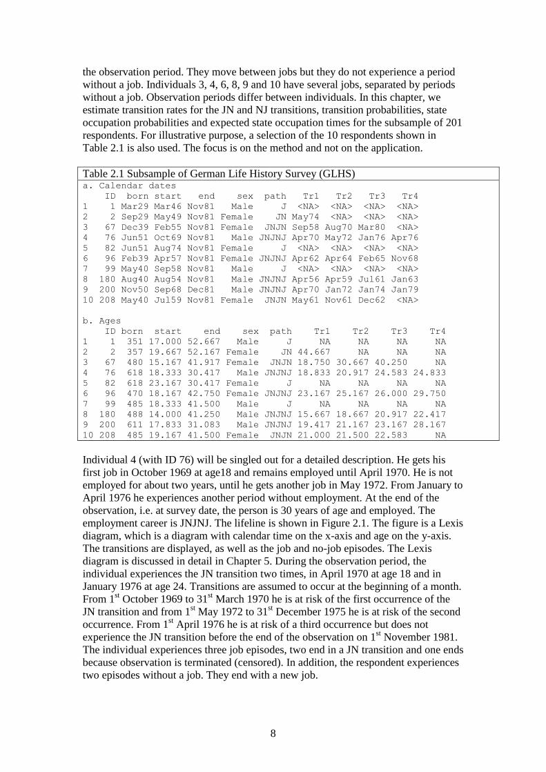
Table 2.1 is also used. The focus is on the method and not on the application.

Table 2.1 Subsample of German Life History Survey (GLHS) a. Calendar dates

ID born start end sex path Tr1 Tr2 Tr3 Tr4

1 1 Mar29 Mar46 Nov81 Male J <NA> <NA> <NA> <NA>

2 2 Sep29 May49 Nov81 Female JN May74 <NA> <NA> <NA>

3 67 Dec39 Feb55 Nov81 Female JNJN Sep58 Aug70 Mar80 <NA>

4 76 Jun51 Oct69 Nov81 Male JNJNJ Apr70 May72 Jan76 Apr76

5 82 Jun51 Aug74 Nov81 Female J <NA> <NA> <NA> <NA>

6 96 Feb39 Apr57 Nov81 Female JNJNJ Apr62 Apr64 Feb65 Nov68

7 99 May40 Sep58 Nov81 Male J <NA> <NA> <NA> <NA>

8 180 Aug40 Aug54 Nov81 Male JNJNJ Apr56 Apr59 Jul61 Jan63

9 200 Nov50 Sep68 Dec81 Male JNJNJ Apr70 Jan72 Jan74 Jan79

10 208 May40 Jul59 Nov81 Female JNJN May61 Nov61 Dec62 <NA>

b. Ages

ID born start end sex path Tr1 Tr2 Tr3 Tr4

1 1 351 17.000 52.667 Male J NA NA NA NA

2 2 357 19.667 52.167 Female JN 44.667 NA NA NA

3 67 480 15.167 41.917 Female JNJN 18.750 30.667 40.250 NA

4 76 618 18.333 30.417 Male JNJNJ 18.833 20.917 24.583 24.833

5 82 618 23.167 30.417 Female J NA NA NA NA

6 96 470 18.167 42.750 Female JNJNJ 23.167 25.167 26.000 29.750

7 99 485 18.333 41.500 Male J NA NA NA NA

8 180 488 14.000 41.250 Male JNJNJ 15.667 18.667 20.917 22.417

9 200 611 17.833 31.083 Male JNJNJ 19.417 21.167 23.167 28.167

10 208 485 19.167 41.500 Female JNJN 21.000 21.500 22.583 NA

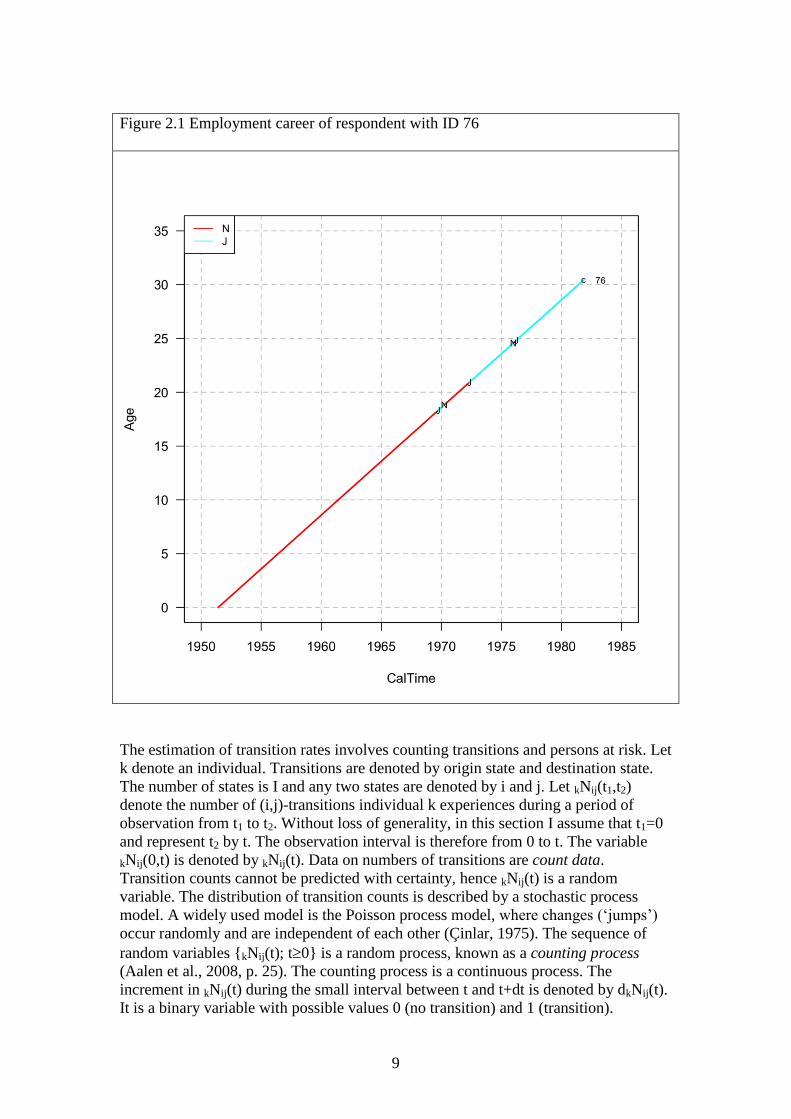
Individual 4 (with ID 76) will be singled out for a detailed description. He gets his

first job in October 1969 at age18 and remains employed until April 1970. He is not

employed for about two years, until he gets another job in May 1972. From January to

April 1976 he experiences another period without employment. At the end of the

observation, i.e. at survey date, the person is 30 years of age and employed. The

employment career is JNJNJ. The lifeline is shown in Figure 2.1. The figure is a Lexis

diagram, which is a diagram with calendar time on the x-axis and age on the y-axis.

The transitions are displayed, as well as the job and no-job episodes. The Lexis

diagram is discussed in detail in Chapter 5. During the observation period, the

individual experiences the JN transition two times, in April 1970 at age 18 and in

January 1976 at age 24. Transitions are assumed to occur at the beginning of a month.

From 1st October 1969 to 31

st March 1970 he is at risk of the first occurrence of the

JN transition and from 1st May 1972 to 31

st December 1975 he is at risk of the second

occurrence. From 1st April 1976 he is at risk of a third occurrence but does not

experience the JN transition before the end of the observation on 1st November 1981.

The individual experiences three job episodes, two end in a JN transition and one ends

because observation is terminated (censored). In addition, the respondent experiences

two episodes without a job. They end with a new job.

9

Figure 2.1 Employment career of respondent with ID 76

The estimation of transition rates involves counting transitions and persons at risk. Let

k denote an individual. Transitions are denoted by origin state and destination state.

The number of states is I and any two states are denoted by i and j. Let kNij(t1,t2)

denote the number of (i,j)-transitions individual k experiences during a period of

observation from t1 to t2. Without loss of generality, in this section I assume that t1=0

and represent t2 by t. The observation interval is therefore from 0 to t. The variable

kNij(0,t) is denoted by kNij(t). Data on numbers of transitions are count data.

Transition counts cannot be predicted with certainty, hence kNij(t) is a random

variable. The distribution of transition counts is described by a stochastic process

model. A widely used model is the Poisson process model, where changes (‘jumps’)

occur randomly and are independent of each other (Çinlar, 1975). The sequence of

random variables {kNij(t); t0} is a random process, known as a counting process

(Aalen et al., 2008, p. 25). The counting process is a continuous process. The

increment in kNij(t) during the small interval between t and t+dt is denoted by dkNij(t).

It is a binary variable with possible values 0 (no transition) and 1 (transition).

10

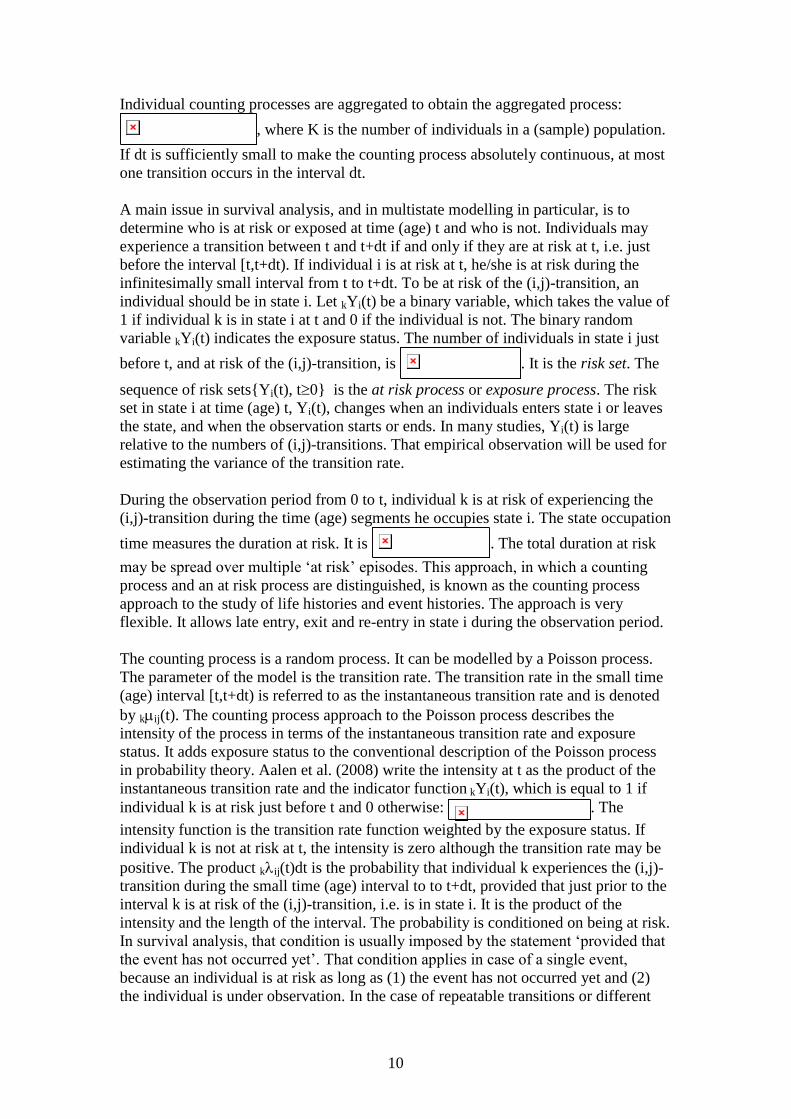
Individual counting processes are aggregated to obtain the aggregated process:

, where K is the number of individuals in a (sample) population.

If dt is sufficiently small to make the counting process absolutely continuous, at most

one transition occurs in the interval dt.

A main issue in survival analysis, and in multistate modelling in particular, is to

determine who is at risk or exposed at time (age) t and who is not. Individuals may

experience a transition between t and t+dt if and only if they are at risk at t, i.e. just

before the interval [t,t+dt). If individual i is at risk at t, he/she is at risk during the

infinitesimally small interval from t to t+dt. To be at risk of the (i,j)-transition, an

individual should be in state i. Let kYi(t) be a binary variable, which takes the value of

1 if individual k is in state i at t and 0 if the individual is not. The binary random

variable kYi(t) indicates the exposure status. The number of individuals in state i just

before t, and at risk of the (i,j)-transition, is . It is the risk set. The

sequence of risk sets{Yi(t), t0} is the at risk process or exposure process. The risk

set in state i at time (age) t, Yi(t), changes when an individuals enters state i or leaves

the state, and when the observation starts or ends. In many studies, Yi(t) is large

relative to the numbers of (i,j)-transitions. That empirical observation will be used for

estimating the variance of the transition rate.

During the observation period from 0 to t, individual k is at risk of experiencing the

(i,j)-transition during the time (age) segments he occupies state i. The state occupation

time measures the duration at risk. It is . The total duration at risk

may be spread over multiple ‘at risk’ episodes. This approach, in which a counting

process and an at risk process are distinguished, is known as the counting process

approach to the study of life histories and event histories. The approach is very

flexible. It allows late entry, exit and re-entry in state i during the observation period.

The counting process is a random process. It can be modelled by a Poisson process.

The parameter of the model is the transition rate. The transition rate in the small time

(age) interval [t,t+dt) is referred to as the instantaneous transition rate and is denoted

by kij(t). The counting process approach to the Poisson process describes the

intensity of the process in terms of the instantaneous transition rate and exposure

status. It adds exposure status to the conventional description of the Poisson process

in probability theory. Aalen et al. (2008) write the intensity at t as the product of the

instantaneous transition rate and the indicator function kYi(t), which is equal to 1 if

individual k is at risk just before t and 0 otherwise: . The

intensity function is the transition rate function weighted by the exposure status. If

individual k is not at risk at t, the intensity is zero although the transition rate may be

positive. The product kij(t)dt is the probability that individual k experiences the (i,j)-

transition during the small time (age) interval to to t+dt, provided that just prior to the

interval k is at risk of the (i,j)-transition, i.e. is in state i. It is the product of the

intensity and the length of the interval. The probability is conditioned on being at risk.

In survival analysis, that condition is usually imposed by the statement ‘provided that

the event has not occurred yet’. That condition applies in case of a single event,

because an individual is at risk as long as (1) the event has not occurred yet and (2)

the individual is under observation. In the case of repeatable transitions or different

11

types of transitions, an individual may be under observation but not at risk. In the

example of employment, an individual in state N is under observation but not at risk

of the JN transition.

If at most one transition occurs during the interval dt, the probability of occurrence

may be expressed in different but equivalent ways. It is the probability that kNij(t)

changes to kNij(t)+1; the probability that the transition occurs at t, Pr(d kNij (t)=1); and

the probability that the transition time (age) kTij is in the [t,t+dt) interval: Pr(t kTij <

t+dt). The probability that dkNij(t) is one, Pr(d kNij (t)=1), is equal to the expected

value of dkNij(t), hence kij(t) dt = E[dkNij(t)]. Note that kNij(t) and its increment

dkNij(t) are observations, whereas kij(t) is a model of the increment dkNij(t) (Poisson

process model that satisfies the two conditions listed above). kij(t) is the intensity

process of the counting process kNij(t).

If individuals are independent of each other, the intensity process of the aggregated

counting process Nij(t) is . If in addition all individuals are

assumed to have the same hazard rate, i.e. for all k, then the survival

times are independent and identically distributed. The aggregate intensity process may

be written as: , where Yi(t) is

the number of individuals in state i just before t. It is the population at risk. The model

is the multiplicative intensity model for a counting process (Aalen

et al., 2008, p. 34). In the multiplicative intensity model, the at risk process Yi(t) does

not depend on unknown parameters (Aalen et al., 2008, p. 77). That condition is

satisfied if the population at risk is large relative to the number of transitions. The

same condition was introduced by Holford (1980) and Laird and Olivier (1981) in the

context of estimating (piecewise-constant) transition rates with log-linear models. The

transition rates ij(t) are key model parameters and a main aim of statistical analysis is

to determine how they vary over time (age) and depend on covariates.

The observed increment dNij(t) of the counting process Nij(t) generally differs from

the model estimate ij(t)dt because observations do not meet the conditions imposed

by the Poisson process. Aalen et al. (2008, p. 27) refer to the difference as noise and

to the probability of a transition during the interval dt as signal. The noise cumulated

up to time (age) t is the martingale Mij(t) and dMij(t) is the increment in noise during

the small interval following t: dMij(t) = dNij(t) - ij(t) dt. The intensity process and the

noise process are stochastic processes, whereas Nij(t) represents observations. Note

that , and , where ij(t) is

the cumulative intensity process, that is the expected number of transitions up to t,

predicted by the Poisson model. The martingale is the difference between the

counting process and the cumulative intensity process. It can be interpreted as

cumulative noise. The intensity process is central to the statistical modelling of event

occurrences and transitions between states. Note that the intensity process depends on

the transition rate and the at risk process.

A frequently used measure in multistate modelling is the cumulative hazard

, where is equal to the increment in the cumulative hazard

12

during an infinitesimally small interval. In case of a continuous process,

. The reason for using the cumulative hazard is given above. The

transition rates ij(t) and the cumulative transition rates Aij(t) are estimated from the

data. The estimation method is determined by the assumed underlying stochastic

process. In this chapter, two methods are described. In the first method, no

assumption is made about the process. The method is knows as the non-parametric

method, because of the absence of a parametric model that described the time (age)

dependence of transition rates. The second method assumes that transition rates are

(piecewise) constant. As a consequence, the duration to the next transition and the

time between two consecutive transitions follow a (piecewise) exponential

distribution. In the remainder of this chapter, I use age as time scale.

a. Non-parametric method

Recall that Nij(t) is the number of (i,j)-transitions experienced by individuals in the

(sample) population during the observation interval from 0 to t and Tij is the age of an

(i,j)-transition. For the estimation of empirical transition rates (non-parametric),

transitions are ordered by age of occurrence. Let denote the age of the n-th

occurrence of the (i,j)-transition experienced in the (sample) population. The number

of individuals at risk just before is . Consider the age interval [t,t+dt). If in a

population no event occurs in the interval, the natural estimate of is zero. If

a transition is recorded during the interval, the natural estimate is 1 divided by the

number of individuals at risk, that is 1/Yi(t) or the proportion of individuals at risk

that experiences a transition. Aggregating these contributions over all age intervals at

which transitions occur, up to age t, gives the estimator of Aij(t). A natural

estimator of the cumulative transition rate at age t is , where

numerator and denominator are aggregations over all individuals. If transition ages

are , then the estimator is , where is the age at the n-th

occurrence of the (i,j)-transition. The estimator is known as the Nelson-Aalen

estimator. The estimator was initially developed by Nelson and extended to event

history models and Markov processes by Aalen, who adopted a counting process

formulation (see Aalen et al., 2008, pp. 70ff). The Nelson-Aalen estimator

corresponds to the cumulative hazard of a discrete distribution, with all its probability

mass concentrated at the observed ages at transition. The matrix is a matrix of

step functions with jumps at ages at transition.

The variance of the Nelson-Aalen estimator is (Aalen

variance). The variance increases with t. The increment is . In

large samples, the Nelson-Aalen estimator at age t is approximately normally

distributed. Therefore the 95 percent confidence interval is . If the

sample size is small, the approximation to the normal distribution is improved by

using a log-transformation giving the confidence interval

13

(Aalen et al., 2008, p. 72).

Consider the employment careers of the 10 individuals, shown in Table 2.1. To track

individuals at risk, ages at entry into observation and exit from observation, and ages

at transition should be ordered. Individual 8 enters observation at age 14.00, followed

by individual 3 at age 15.16. The first transition occurs at age 15.67 when individual 8

enters a period without a job. At that age, 2 individuals are at risk of the JN transition

(3 and 8). The Nelson-Aalen estimator of the cumulative transition rate at that age is

½. The next event is at age 17.00 when individual 1 enters observation. Just before

that age, individual 3 is at risk in J and individual 8 in N. At age 17.00, individual 1

joins 3 in J. The next event is at age 17.83 when individual 9 enters observation.

When individual 6 enters observation at age 18.17, three individuals are in J and one

in N. Individuals 4 and 7 enter observation at age 18.33. At age 18.67, individual 8

enters J again. Just before that age, he is the only person in N and at risk of the NJ

transition, while 6 individuals are in J. Hence the estimator of the hazard is 1. The

next event is at age 18.75,when individual 3 leaves J and enters a period without a

job. At that age 7 individuals are in J and at risk of the JN transition (1,3,4,6,7,8,9).

The cumulative JN transition rate 1/2 +1/7=0.64. The Aalen variance is (1/2)2 + (1/7)

2 =0.270. At that age, three individuals have not yet entered observation and do not

contribute to the cumulative hazard estimation (2,5 and 10). The cumulative transition

rate increases to age 44.67 when individual 3 enters a period without a job. At that

age, the cumulative transition rate is 2.696 and the Aalen variance is 0.764. Table 2.2

shows the Nelson-Aalen estimator based on data of the 10 respondents. The columns

are: (1) age at entry into observation, exit from observation or transition, (2) the

population at risk just prior to the transition (nrisk), (3) occurrence of a transition

(nevent), (4) censoring (ncens), (5) the Nelson-Aalen estimator of the cumulative

transition rate (cumhaz) at the indicated age, (6) the Aalen estimator of the variance

(var)and (7) increment in the cumulative hazard (delta). The information is

shown each time a transition occurs or a respondent enters or leaves observation. The

number of events is less than the number of entries (10) + the number of exits (10) +

the number of JN transitions (13) + the number of NJ transitions (10), because

individuals 3 and 7 enter observation at the same time, individual 5 enters observation

when individuals 6 and 9 experience a JN transition, and individuals 4 and 5 leave

observation at the same age, as do individuals 7 and 10. The table is produced by the

mvna function of the mvna package. The last column is produced by the etm

function of the etm package (see below). The object d.10 is the Biograph object for a

selection of 10 respondents and D$D is an object with data of 10 respondents in mvna

format. The following code is used:

# Select 10 respondents and create Biograph object

idd <- c(1,2,67,76,82,96,99,180,200,208)

d.10 <- d3.a[d3.a$ID%in%idd,]

D<- Biograph.mvna (d.10)

library (mvna)

library (etm)

tra <- matrix(ncol=2,nrow=2,FALSE)

tra[1, 2] <- TRUE

tra[2,1] <- TRUE

na <- mvna(data=D$D,c("J","N"),tra,"cens")

14

etm.0 <- etm(data=D$D,c("J","N"),tra,"cens",s=0)

gg.1 <- data.frame (

round(na$"J N"$time,4),

na$n.risk[,1],

unname(aperm(na$n.event,c(3,2,1))[,2,1]),

na$n.cens[,1],

round(na$"J N"$na,4),

round(na$"J N"$var.aalen,3),

round(aperm (etm.0$delta.na,c(3,2,1))[,2,1],4))

dimnames (gg.1) <- list

(1:37,c("age","nrisk","nevent","ncens","cumhaz","var

","delta"))

gg.2 <- data.frame (

round(na$"N J"$time,4),

na$n.risk[,2][na$time %in% na$"N J"$time],

unname(aperm(na$n.event,c(3,2,1))[,1,2])[na$time

%in% na$"N J"$time],

na$n.cens[,2][na$time %in% na$"N J"$time],

round(na$"N J"$na,4),

round(na$"N J"$var.aalen,3),

round(aperm

(etm.0$delta.na,c(3,2,1))[,1,2][na$time %in%

na$"N J"$time],4))

dimnames (gg.2) <- list

(1:nrow(gg.2),c("age","nrisk","nevent","ncens","cumh

az","var","delta"))

The 10 respondents enter observation at ages 14.00 (ID 180), 15.67 (ID 67), 17.00 (ID

1), 17.83 (ID 200), 18.17 (ID 96), 18.83 (ID 99), 19.17 (ID 208), 19.67 (ID 2) and

23.17 (ID 82) (see Table 2.1). They experience 13 JN transitions and 10 NJ

transitions. At time of survey, 7 respondents had a job and 3 were without a job. The

youngest age at job exit is 15.67 years (ID 180). The youngest age at survey is 30.42

(ID 76 and 82) and the highest is 52.67 (ID 1). Two respondents are 41.50 years at

survey date, one (ID 99) has a job and one (ID 208) is without a job.

15

Table 2.2 Nelson-Aalen estimator and Aalen variance of cumulative transition rates.

GLHS, subsample of 10 respondents. Transition JN

age nrisk nevent ncens cumhaz var delta

1 14.0000 1 0 0 0.0000 0.000 0.0000

2 15.1667 1 0 0 0.0000 0.000 0.0000

3 15.6667 2 1 0 0.5000 0.250 0.5000

4 17.0000 1 0 0 0.5000 0.250 0.0000

5 17.8333 2 0 0 0.5000 0.250 0.0000

6 18.1667 3 0 0 0.5000 0.250 0.0000

7 18.3333 4 0 0 0.5000 0.250 0.0000

8 18.6667 6 0 0 0.5000 0.250 0.0000

9 18.7500 7 1 0 0.6429 0.270 0.1429

10 18.8333 6 1 0 0.8095 0.298 0.1667

11 19.1667 5 0 0 0.8095 0.298 0.0000

12 19.4167 6 1 0 0.9762 0.326 0.1667

13 19.6667 5 0 0 0.9762 0.326 0.0000

14 20.9167 6 1 0 1.1429 0.354 0.1667

15 21.0000 6 1 0 1.3095 0.382 0.1667

16 21.1667 5 0 0 1.3095 0.382 0.0000

17 21.5000 6 0 0 1.3095 0.382 0.0000

18 22.4167 7 0 0 1.3095 0.382 0.0000

19 22.5833 8 1 0 1.4345 0.397 0.1250

20 23.1667 7 2 0 1.7202 0.438 0.2857

21 24.5833 6 1 0 1.8869 0.466 0.1667

22 24.8333 5 0 0 1.8869 0.466 0.0000

23 25.1667 6 0 0 1.8869 0.466 0.0000

24 26.0000 7 1 0 2.0298 0.486 0.1429

25 28.1667 6 0 0 2.0298 0.486 0.0000

26 29.7500 7 0 0 2.0298 0.486 0.0000

27 30.4167 8 0 2 2.0298 0.486 0.0000

28 30.6667 6 0 0 2.0298 0.486 0.0000

29 31.0833 7 0 1 2.0298 0.486 0.0000

30 40.2500 6 1 0 2.1964 0.514 0.1667

31 41.2500 5 0 1 2.1964 0.514 0.0000

32 41.5000 4 0 1 2.1964 0.514 0.0000

33 41.9167 3 0 0 2.1964 0.514 0.0000

34 42.7500 3 0 1 2.1964 0.514 0.0000

35 44.6667 2 1 0 2.6964 0.764 0.5000

36 52.1667 1 0 0 2.6964 0.764 0.0000

37 52.6667 1 0 1 2.6964 0.764 0.0000

Transition NJ

age nrisk nevent ncens cumhaz var delta

1 17.0000 1 0 0 0.0000 0.000 0.0000

2 17.8333 1 0 0 0.0000 0.000 0.0000

3 18.1667 1 0 0 0.0000 0.000 0.0000

4 18.3333 1 0 0 0.0000 0.000 0.0000

5 18.6667 1 1 0 1.0000 1.000 1.0000

6 18.8333 1 0 0 1.0000 1.000 0.0000

7 19.1667 2 0 0 1.0000 1.000 0.0000

8 19.4167 2 0 0 1.0000 1.000 0.0000

9 19.6667 3 0 0 1.0000 1.000 0.0000

10 20.9167 3 1 0 1.3333 1.111 0.3333

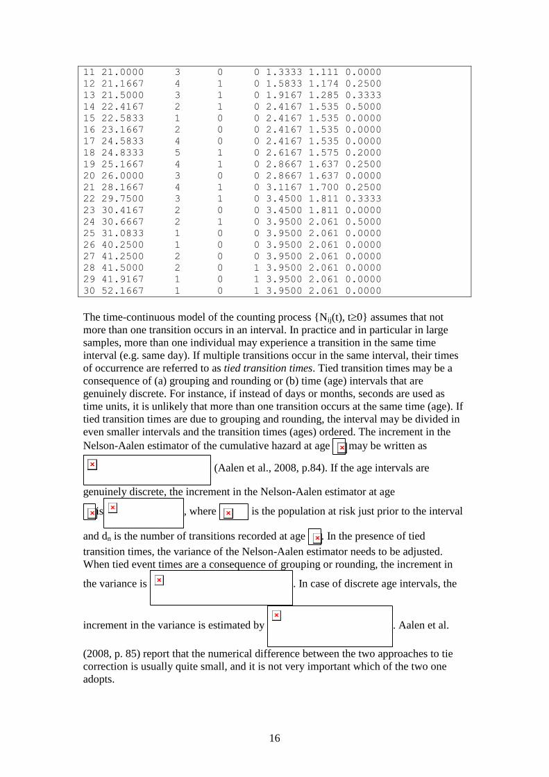
16

11 21.0000 3 0 0 1.3333 1.111 0.0000

12 21.1667 4 1 0 1.5833 1.174 0.2500

13 21.5000 3 1 0 1.9167 1.285 0.3333

14 22.4167 2 1 0 2.4167 1.535 0.5000

15 22.5833 1 0 0 2.4167 1.535 0.0000

16 23.1667 2 0 0 2.4167 1.535 0.0000

17 24.5833 4 0 0 2.4167 1.535 0.0000

18 24.8333 5 1 0 2.6167 1.575 0.2000

19 25.1667 4 1 0 2.8667 1.637 0.2500

20 26.0000 3 0 0 2.8667 1.637 0.0000

21 28.1667 4 1 0 3.1167 1.700 0.2500

22 29.7500 3 1 0 3.4500 1.811 0.3333

23 30.4167 2 0 0 3.4500 1.811 0.0000

24 30.6667 2 1 0 3.9500 2.061 0.5000

25 31.0833 1 0 0 3.9500 2.061 0.0000

26 40.2500 1 0 0 3.9500 2.061 0.0000

27 41.2500 2 0 0 3.9500 2.061 0.0000

28 41.5000 2 0 1 3.9500 2.061 0.0000

29 41.9167 1 0 1 3.9500 2.061 0.0000

30 52.1667 1 0 1 3.9500 2.061 0.0000

The time-continuous model of the counting process {Nij(t), t0} assumes that not

more than one transition occurs in an interval. In practice and in particular in large

samples, more than one individual may experience a transition in the same time

interval (e.g. same day). If multiple transitions occur in the same interval, their times

of occurrence are referred to as tied transition times. Tied transition times may be a

consequence of (a) grouping and rounding or (b) time (age) intervals that are

genuinely discrete. For instance, if instead of days or months, seconds are used as

time units, it is unlikely that more than one transition occurs at the same time (age). If

tied transition times are due to grouping and rounding, the interval may be divided in

even smaller intervals and the transition times (ages) ordered. The increment in the

Nelson-Aalen estimator of the cumulative hazard at age may be written as

(Aalen et al., 2008, p.84). If the age intervals are

genuinely discrete, the increment in the Nelson-Aalen estimator at age

is , where is the population at risk just prior to the interval

and dn is the number of transitions recorded at age . In the presence of tied

transition times, the variance of the Nelson-Aalen estimator needs to be adjusted.

When tied event times are a consequence of grouping or rounding, the increment in

the variance is . In case of discrete age intervals, the

increment in the variance is estimated by . Aalen et al.

(2008, p. 85) report that the numerical difference between the two approaches to tie

correction is usually quite small, and it is not very important which of the two one

adopts.

17

b. Parametric method: exponential and piecewise exponential models

The Nelson-Aalen estimator is nonparametric. The shape of the hazard function is not

constrained in any way. In a parametric counting process model, the age dependence

of the transition rate is constrained and consequently the waiting times to a transition

are constrained. It is assumed that there is a continuous-time process underlying the

data. In addition, the transition rate may depend on covariates. Covariates are not

considered in this chapter. Two models are considered in this chapter. The first is the

exponential model, which imposes a constant transition rate and an exponential

waiting time distribution. The second model is a piecewise exponential model, which

imposes piecewise-constant transition rates. Transitions rates are assumed to be

constant in age intervals of usually one year. The transition rates of consecutive age

groups are unrelated, i.e. no restrictions are imposed on how the piecewise-constant

rates vary with age. The estimation method therefore combines a parametric approach

(within intervals) and a non-parametric approach (between intervals). Individuals are

assumed to be independent and to have the same instantaneous transition rate. In other

words, transition times of the individuals in the (sample) population are assumed to be

independent and identically distributed. The estimation of piecewise exponential

models and occurrence-exposure rates received considerable attention in the literature

(see e.g. Hoem and Funck Jensen, 1982, Tuma and Hannan, 1984, Hougaard, 2000,

Blossfeld and Rohwer, 2002, Aalen et al., 2008, Van den Hout and Matthews, 2008,

Li et al., 2012). Mamun (2003) and Reuser et al. (2010), who study the effect of

covariates on disability and mortality, impose the restriction that the piecewise-

constant transition rates (occurrence-exposure rates) increase exponentially with age.

The result is a Gompertz model with piecewise constant transition rates. The choice

of model is determined by the age profile of transition rates (exponential increase) and

data limitations. Parametric models of transition rates covering the entire age range in

multistate models have been estimated too. Van den Hout and Matthews (2008)

estimate a multistate model in which the age dependence of transition rates is

described by a Weibull model and Van den Hout et al. (2014) use a Gompertz model.

In demography, a variety of models are specified to describe age profiles of transition

rates in multistate models. For an overview of models, see Rogers (1986).

In the counting process approach, the likelihood function is written in terms of the

counting process kNij(t) and the intensity process kij(t), where t represents age. The

intensity process at age t is . The indicator function kYi(t) is 1 if

individual k is under observation and in state i at t and 0 otherwise. The total

occupation time in state i is , with the highest age. If individuals

are independent, the intensity process at age t is and is

the number of (i,j)-transitions between t and t+dt, given the instantaneous transition

rate ant the exposure function. If in addition all individuals have the same hazard rate,

i.e. for all k, then the survival times are independent and identically

distributed. The aggregate intensity process may be written as:

, where Yi(t) is the number of

individuals under observation and in state i just before t. If the transition rate is

constant, then kij(t)= kij for all t and the intensity process at t is . If

18

the transition rate is piecewise-constant during the age interval from x to x+1, kij(t)=

kij(x) for x t < x+1 and the intensity process at t is for x t <

x+1. The intensity of leaving state i at age t, irrespective of destination, is

, which may be written as , with

.

Let denote the highest age in the study. A transition is observed if it occurs before

. Individual k experiences kNij() occurrences of the (i,j)-transition from 0 to . In

addition, the observation is censored in state i or in another state. Hence, the number

of episodes of exposure is the number of transitions plus one. The contribution of

individual k to the likelihood function is

where is the age at the n-th occurrence of the (i,j)-transition. Since the intensity

depends on the instantaneous transition rate and exposure, the likelihood function is

written in terms of the counting process kNij(t) and its intensity process kij(t) (Aalen

et al., 2008, p. 210). Notice that , with the at risk function

equal to one if individual k is in state i just before the transition and 0 otherwise, and

, with the at risk function equal to one if k is in i at . The last term

is the probability of surviving in state i between the age at last entry and age at

censoring. The intensity depends on the instantaneous rate of leaving i and the

at risk function, which is zero except for larger than or equal to the age of the last

transition and less than the age at censoring. In the traditional approach, integration is

from the beginning of the period during which individual k is at risk of the (i,j)-

transition to the end of that period. In the first term, the end is the age at the next

occurrence; in the last term, it is the age at censoring. Hougaard (2000, p. 181) derives

the likelihood function following the traditional approach:

where is one if the at risk period ends in an (i,j)-transition and zero if it ends

because the observation is discontinued (censored). The counting process approach to

the likelihood function is (Aalen et al., 2008, p. 210):

with kNij(t) the increment of kNij at age t.

The full likelihood is

19

with i() the intensity process of the aggregated process Ni(t).

The log-likelihood is . The

maximum likelihood estimator of ij is the value of ij for which the score function is

zero: . The score function is the first-order condition for maximizing

the likelihood that the model predicts the data. In the exponential model,

and the first term of the log-likelihood is

. The second term is

, with Ri() the total exposure time in state i for all

individuals in the (sample) population. The score function is

. The solution of the equation gives the

maximum likelihood estimator of the transition rate: . The estimator

is the observed number of transitions (occurrences) divided by the total duration at

risk (exposure). The estimator is an occurrence-exposure rate.

In large samples, the estimator is approximately normally distributed around the

true value of ij, with the variance estimator . To improve the

distribution for , the logarithmic transformation is used. Only 10 transitions are

needed for to be approximately normally distributed around with

variance estimator (Aalen et al., 2008, p. 215).

The cumulative transition rate under the exponential model (occurrence-exposure

rate) increases linearly with duration. The empirical cumulative transition rate

(Nelson-Aalen estimator) is a step function (Andersen and Keiding, 2002, p. 100).

The two estimators are usually close. To improve the approximation, the age interval

from 0 to may be partitioned in subintervals and the occurrence-exposure rate

estimated for each subinterval. The exponential model turns into a piecewise

exponential model with piecewise-constant transition rates. That is the common

approach in demography, where an age intervals is usually one year. The estimator of

the transition rate and the variance, given above, are applied to each subinterval.

Consider the aggregate counting processes Nij(t) and Yi(t), and subintervals from

exact age x to exact age y (y not included). Age intervals are usually one year, but a

more general interval is chosen here. The transition rate, which is constant in the

interval, is denoted by . The observed number of (i,j)-transitions during the

interval is and the observed exposure time in state i is . Following

Aalen et al. (2008, pp. 220ff), the score function is solved. The score function is

, where

20

and with an indicator function taking the value of one

in the interval from x to y and a value of zero otherwise.

The maximum likelihood estimator of the transition rate from i to j during the interval

from x to y is the occurrence-exposure rate . Occurrence-

exposure rates are approximately independent and normally distributed around their

true values, and the variance of can be estimated by or the

logarithmic transformation . In demography,

epidemiology and actuarial science, transition rates are usually occurrence-exposure

rates and are determined by dividing occurrences by exposures. In the absence of

exposure data, exposure is approximated by the product of the mid-period population

and the length of the period, a method also used by Aalen et al. (2008, p. 222).

By way of illustration of the method, aggregate transition rates and age-specific

transition rates are estimated from the subsample of 201 individuals, entering

observation at labour market entry. The analysis focuses on transitions between job

episodes and episodes without a job. Transitions between jobs are omitted. Biograph

and some additional calculations produced the main results reported in this section.

The results are compared to those generated by the msm package for multistate

modelling. The 201 individuals experience 504 episodes (323 job episodes and 181

episodes without a job). The total observation time between first job entry and survey

is 4,668 person-years (3,397 person-years in J and 1,271 person-years in N). The

sample population experienced 303 transitions during the observation period (181 JN

transitions and 122 NJ transitions). The JN transition rate is 181/3397 = 0.0533 per

year and the NJ transition rate is 122/1271=0.0960 per year. To determine the 95

percent confidence interval of the occurrence-exposure rate. The log-transformation

of the estimator is used: . The confidence interval around

the JN transition rate is , which is (0.0461, 0.0617).

The confidence interval around the NJ transition rate is

, which is (0.0804, 0.1146). Bootstrapping, i.e.

sampling the original 201 observations with replacement, with 100 bootstrap samples,

produces a JN transition rate of 0.0535 with confidence interval (0.0452, 0.0636) and

a NJ transition rate of 0.0977 with confidence interval (0.0701, 0.1264). 500 bootstrap

samples yield a JN transition rate of 0.0534 with confidence interval (0.0.0451,

0.0629) and a NJ transition rate of 0.0973 with confidence interval (0.0729, 0.1254).

Bootstrapping produces confidence intervals that are somewhat larger than the

analytical method.

The package msm produces the same estimates and confidence intervals. The code is:

library (msm)

d <- Remove.intrastate(GLHS)

dd <- ChangeObservationWindow.e

(Bdata=d,entrystate="J",exitstate=NA)

data <- date_b (Bdata=dd,selectday=1,format.out="age",

21

covs=c("marriage","LMentry"))

Dmsm <- Biograph.msm(data)

twoway2.q <- rbind(c(-0.025, 0.025),c(0.2,-0.2))

crudeinits.msm(state ~ date, ID, data=Dmsm,

qmatrix=twoway2.q)

GLHS.msm.y <- msm( state ~ date,

subject=ID,

data = Dmsm,

use.deriv=TRUE,

exacttimes=TRUE,

qmatrix = twoway2.q,

obstype=2,

control=list(trace=2,REPORT=1,

abstol=0.0000005),

method="BFGS")

The first line removes transitions between jobs. The second line changes the

observation window: observation starts at labour market entry (first job) and ends at

interview. The third line converts dates in CMC into ages. The fourth line converts

the Biograph object data to the long format required by the msm package. The fifth

and sixth lines generate initial values for transition rates. The next line calls the msm

function for estimating the transition rates. Object GLHS.msm.y contains the

estimates and the 95% confidence intervals, with the row variable denoting origin

and the column variable destination. State 1 is J and state 2 is N.

State 1 State 2

State 1 -0.05328 (-0.06164,-0.04606) 0.05328 (0.04606,0.06164)

State 2 0.09602 (0.08041,0.1147) -0.09602 (-0.1147,-0.08041)

As expected, the 95% confidence intervals produced by the msm package are the

same as computed above. The msm package includes a function (boot) that uses

bootstrapping to produce estimates, standard errors and confidence intervals.

Bootstrapping, with 100 bootstrap samples, produces the following estimates and

confidence intervals: 0.0532 for the JN transition rate, with 95% confidence interval

(0.0453, 0.0621), and 0.0988 for the NJ transition rate, with 95% confidence interval

(0.0755, 0.1294).

Consider the piecewise constant exponential model with age intervals of one year.

The input data are transition counts (occurrences) and exposures by single year of age

for the 201 respondents. Transition counts and exposure times are shown in Table 2.3.

Column JN shows the number of transitions from J to N and PY is the exposure time.

The table also shows the state occupancies at birthdays (Occup) and the number of

observations censured by age (cens). The estimate of the transition rate is r.est and

the 95% confidence interval is (r.L95, r.U95). The estimate and the confidence

interval are obtained using the analytical method. Bootstrapping produces the estimate

b.est and the confidence interval (b.L95, b.U95). The cumulative transition rate

is cumrate. Consider age 30. Of the 201 individuals, 198 are under observation at

that age; 138 have a job on their 30th

birthday and 60 are without a job. For 3

individuals, the information is missing. Two did not reach age 30 yet when

observation ended at age at interview (ID 45 and 115) and one entered labour force

and observation after age 30 (ID 49). Together the individuals spent 127.75 years in

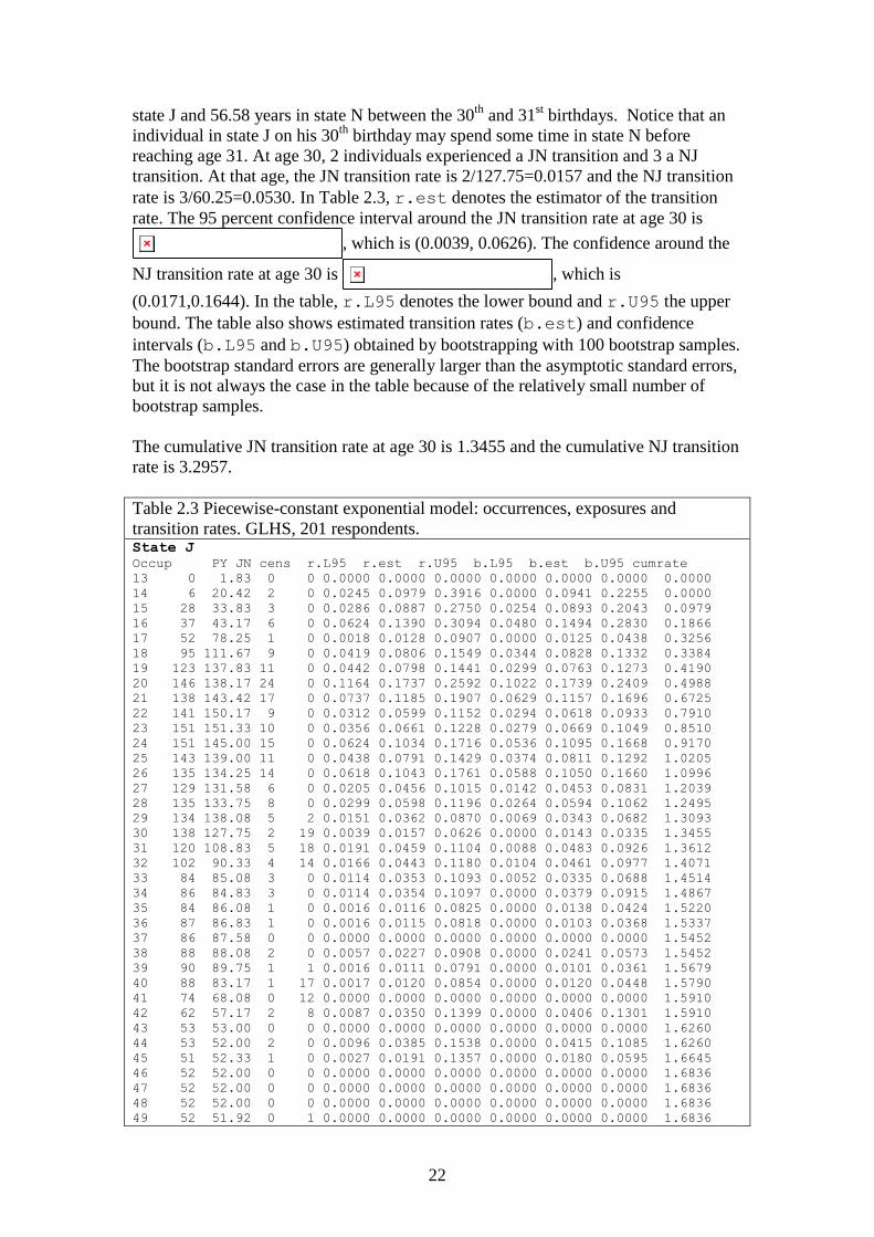
22

state J and 56.58 years in state N between the 30th

and 31st birthdays. Notice that an

individual in state J on his 30th

birthday may spend some time in state N before

reaching age 31. At age 30, 2 individuals experienced a JN transition and 3 a NJ

transition. At that age, the JN transition rate is 2/127.75=0.0157 and the NJ transition

rate is 3/60.25=0.0530. In Table 2.3, r.est denotes the estimator of the transition

rate. The 95 percent confidence interval around the JN transition rate at age 30 is

, which is (0.0039, 0.0626). The confidence around the

NJ transition rate at age 30 is , which is

(0.0171,0.1644). In the table, r.L95 denotes the lower bound and r.U95 the upper

bound. The table also shows estimated transition rates (b.est) and confidence

intervals (b.L95 and b.U95) obtained by bootstrapping with 100 bootstrap samples.

The bootstrap standard errors are generally larger than the asymptotic standard errors,

but it is not always the case in the table because of the relatively small number of

bootstrap samples.

The cumulative JN transition rate at age 30 is 1.3455 and the cumulative NJ transition

rate is 3.2957.

Table 2.3 Piecewise-constant exponential model: occurrences, exposures and

transition rates. GLHS, 201 respondents. State J

Occup PY JN cens r.L95 r.est r.U95 b.L95 b.est b.U95 cumrate

13 0 1.83 0 0 0.0000 0.0000 0.0000 0.0000 0.0000 0.0000 0.0000

14 6 20.42 2 0 0.0245 0.0979 0.3916 0.0000 0.0941 0.2255 0.0000

15 28 33.83 3 0 0.0286 0.0887 0.2750 0.0254 0.0893 0.2043 0.0979

16 37 43.17 6 0 0.0624 0.1390 0.3094 0.0480 0.1494 0.2830 0.1866

17 52 78.25 1 0 0.0018 0.0128 0.0907 0.0000 0.0125 0.0438 0.3256

18 95 111.67 9 0 0.0419 0.0806 0.1549 0.0344 0.0828 0.1332 0.3384

19 123 137.83 11 0 0.0442 0.0798 0.1441 0.0299 0.0763 0.1273 0.4190

20 146 138.17 24 0 0.1164 0.1737 0.2592 0.1022 0.1739 0.2409 0.4988

21 138 143.42 17 0 0.0737 0.1185 0.1907 0.0629 0.1157 0.1696 0.6725

22 141 150.17 9 0 0.0312 0.0599 0.1152 0.0294 0.0618 0.0933 0.7910

23 151 151.33 10 0 0.0356 0.0661 0.1228 0.0279 0.0669 0.1049 0.8510

24 151 145.00 15 0 0.0624 0.1034 0.1716 0.0536 0.1095 0.1668 0.9170

25 143 139.00 11 0 0.0438 0.0791 0.1429 0.0374 0.0811 0.1292 1.0205

26 135 134.25 14 0 0.0618 0.1043 0.1761 0.0588 0.1050 0.1660 1.0996

27 129 131.58 6 0 0.0205 0.0456 0.1015 0.0142 0.0453 0.0831 1.2039

28 135 133.75 8 0 0.0299 0.0598 0.1196 0.0264 0.0594 0.1062 1.2495

29 134 138.08 5 2 0.0151 0.0362 0.0870 0.0069 0.0343 0.0682 1.3093

30 138 127.75 2 19 0.0039 0.0157 0.0626 0.0000 0.0143 0.0335 1.3455

31 120 108.83 5 18 0.0191 0.0459 0.1104 0.0088 0.0483 0.0926 1.3612

32 102 90.33 4 14 0.0166 0.0443 0.1180 0.0104 0.0461 0.0977 1.4071

33 84 85.08 3 0 0.0114 0.0353 0.1093 0.0052 0.0335 0.0688 1.4514

34 86 84.83 3 0 0.0114 0.0354 0.1097 0.0000 0.0379 0.0915 1.4867

35 84 86.08 1 0 0.0016 0.0116 0.0825 0.0000 0.0138 0.0424 1.5220

36 87 86.83 1 0 0.0016 0.0115 0.0818 0.0000 0.0103 0.0368 1.5337

37 86 87.58 0 0 0.0000 0.0000 0.0000 0.0000 0.0000 0.0000 1.5452

38 88 88.08 2 0 0.0057 0.0227 0.0908 0.0000 0.0241 0.0573 1.5452

39 90 89.75 1 1 0.0016 0.0111 0.0791 0.0000 0.0101 0.0361 1.5679

40 88 83.17 1 17 0.0017 0.0120 0.0854 0.0000 0.0120 0.0448 1.5790

41 74 68.08 0 12 0.0000 0.0000 0.0000 0.0000 0.0000 0.0000 1.5910

42 62 57.17 2 8 0.0087 0.0350 0.1399 0.0000 0.0406 0.1301 1.5910

43 53 53.00 0 0 0.0000 0.0000 0.0000 0.0000 0.0000 0.0000 1.6260

44 53 52.00 2 0 0.0096 0.0385 0.1538 0.0000 0.0415 0.1085 1.6260

45 51 52.33 1 0 0.0027 0.0191 0.1357 0.0000 0.0180 0.0595 1.6645

46 52 52.00 0 0 0.0000 0.0000 0.0000 0.0000 0.0000 0.0000 1.6836

47 52 52.00 0 0 0.0000 0.0000 0.0000 0.0000 0.0000 0.0000 1.6836

48 52 52.00 0 0 0.0000 0.0000 0.0000 0.0000 0.0000 0.0000 1.6836

49 52 51.92 0 1 0.0000 0.0000 0.0000 0.0000 0.0000 0.0000 1.6836

23

50 51 37.25 2 26 0.0134 0.0537 0.2147 0.0000 0.0544 0.1249 1.6836

51 24 15.67 0 17 0.0000 0.0000 0.0000 0.0000 0.0000 0.0000 1.7373

52 7 3.33 0 7 0.0000 0.0000 0.0000 0.0000 0.0000 0.0000 1.7373

53 0 0.00 0 0 0.0000 0.0000 0.0000 0.0000 0.0000 0.0000 1.7373

State N

Occup PY NJ cens r.L95 r.est r.U95 b.L95 b.est b.U95 cumrate

13 0 0.00 0 0 0.0000 0.0000 0.0000 0.0000 0.0000 0.0000 0.0000

14 0 0.33 0 0 0.0000 0.0000 0.0000 0.0000 0.0000 0.0000 0.0000

15 2 3.67 0 0 0.0000 0.0000 0.0000 0.0000 0.0000 0.0000 0.0000

16 5 8.25 2 0 0.0606 0.2424 0.9693 0.0000 0.2412 0.6905 0.0000

17 9 8.08 3 0 0.1197 0.3713 1.1512 0.0000 0.4121 1.0889 0.2424

18 7 9.92 3 0 0.0975 0.3024 0.9377 0.0000 0.2947 0.6461 0.6137

19 13 13.67 10 0 0.3936 0.7315 1.3596 0.3920 0.7578 1.1739 0.9161

20 14 26.83 6 0 0.1005 0.2236 0.4978 0.0928 0.2296 0.4226 1.6477

21 32 33.50 11 0 0.1818 0.3284 0.5929 0.1760 0.3322 0.5461 1.8713

22 38 33.75 9 0 0.1387 0.2667 0.5125 0.1203 0.2764 0.4944 2.1996

23 38 41.17 6 0 0.0655 0.1457 0.3244 0.0455 0.1488 0.2946 2.4663

24 42 48.92 6 0 0.0551 0.1226 0.2730 0.0421 0.1317 0.2440 2.6121

25 51 55.00 3 0 0.0176 0.0545 0.1691 0.0000 0.0564 0.1292 2.7347

26 59 60.42 6 0 0.0446 0.0993 0.2210 0.0449 0.1014 0.1646 2.7892

27 67 65.17 9 0 0.0719 0.1381 0.2654 0.0648 0.1457 0.2569 2.8886

28 64 66.00 6 0 0.0408 0.0909 0.2024 0.0297 0.0911 0.1569 3.0267

29 66 61.75 11 0 0.0987 0.1781 0.3217 0.0882 0.1783 0.2794 3.1176

30 60 56.58 3 6 0.0171 0.0530 0.1644 0.0000 0.0523 0.1221 3.2957

31 53 50.83 4 9 0.0295 0.0787 0.2097 0.0198 0.0824 0.1614 3.3487

32 45 45.75 0 3 0.0000 0.0000 0.0000 0.0000 0.0000 0.0000 3.4274

33 46 44.92 5 0 0.0463 0.1113 0.2674 0.0281 0.1060 0.1873 3.4274

34 44 45.17 1 0 0.0031 0.0221 0.1572 0.0000 0.0219 0.0730 3.5387

35 46 43.92 4 0 0.0342 0.0911 0.2427 0.0203 0.0917 0.2204 3.5609

36 43 43.17 0 0 0.0000 0.0000 0.0000 0.0000 0.0000 0.0000 3.6519

37 44 42.42 2 0 0.0118 0.0471 0.1885 0.0000 0.0458 0.1160 3.6519

38 42 41.92 4 0 0.0358 0.0954 0.2542 0.0085 0.0938 0.2038 3.6991

39 40 40.17 0 0 0.0000 0.0000 0.0000 0.0000 0.0000 0.0000 3.7945

40 41 36.25 4 5 0.0414 0.1103 0.2940 0.0263 0.1130 0.2514 3.7945

41 33 30.50 0 5 0.0000 0.0000 0.0000 0.0000 0.0000 0.0000 3.9048

42 28 24.50 1 7 0.0057 0.0408 0.2898 0.0000 0.0463 0.1723 3.9048

43 22 22.00 0 0 0.0000 0.0000 0.0000 0.0000 0.0000 0.0000 3.9457

44 22 23.00 0 0 0.0000 0.0000 0.0000 0.0000 0.0000 0.0000 3.9457

45 24 22.67 2 0 0.0221 0.0882 0.3528 0.0000 0.1051 0.3614 3.9457

46 23 23.00 0 0 0.0000 0.0000 0.0000 0.0000 0.0000 0.0000 4.0339

47 23 23.00 0 0 0.0000 0.0000 0.0000 0.0000 0.0000 0.0000 4.0339

48 23 23.00 0 0 0.0000 0.0000 0.0000 0.0000 0.0000 0.0000 4.0339

49 23 22.92 0 1 0.0000 0.0000 0.0000 0.0000 0.0000 0.0000 4.0339

50 22 17.92 1 10 0.0079 0.0558 0.3962 0.0000 0.0570 0.1755 4.0339

51 13 8.83 0 8 0.0000 0.0000 0.0000 0.0000 0.0000 0.0000 4.0897

52 5 2.00 0 5 0.0000 0.0000 0.0000 0.0000 0.0000 0.0000 4.0897

53 0 0.00 0 0 0.0000 0.0000 0.0000 0.0000 0.0000 0.0000 4.0897

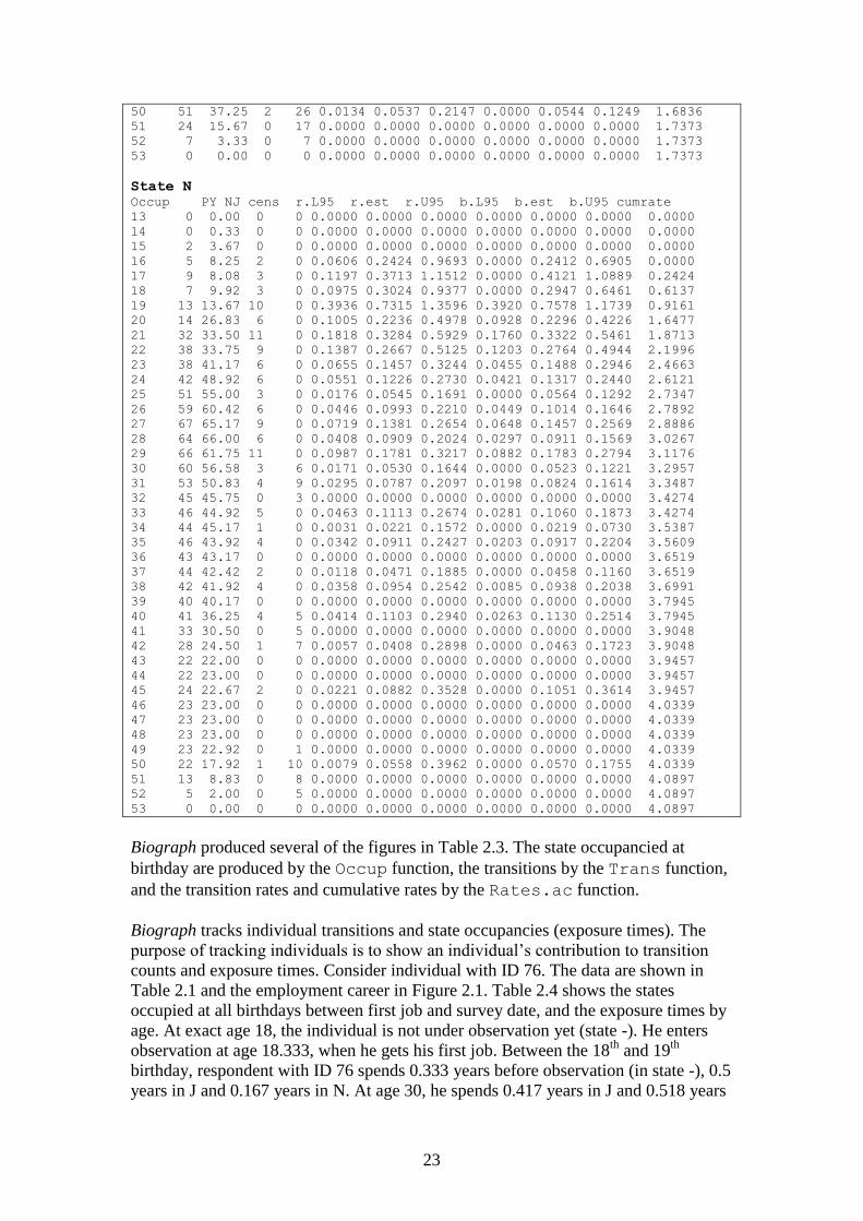
Biograph produced several of the figures in Table 2.3. The state occupancied at

birthday are produced by the Occup function, the transitions by the Trans function,

and the transition rates and cumulative rates by the Rates.ac function.

Biograph tracks individual transitions and state occupancies (exposure times). The

purpose of tracking individuals is to show an individual’s contribution to transition

counts and exposure times. Consider individual with ID 76. The data are shown in

Table 2.1 and the employment career in Figure 2.1. Table 2.4 shows the states

occupied at all birthdays between first job and survey date, and the exposure times by

age. At exact age 18, the individual is not under observation yet (state -). He enters

observation at age 18.333, when he gets his first job. Between the 18th

and 19th

birthday, respondent with ID 76 spends 0.333 years before observation (in state -), 0.5

years in J and 0.167 years in N. At age 30, he spends 0.417 years in J and 0.518 years

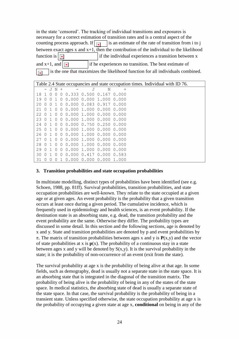
24

in the state ‘censored’. The tracking of individual transitions and exposures is

necessary for a correct estimation of transition rates and is a central aspect of the

counting process approach. If is an estimate of the rate of transition from i to j

between exact ages x and x+1, then the contribution of the individual to the likelihood

function is if the individual experiences a transition between x

and x+1, and if he experiences no transition. The best estimate of

is the one that maximizes the likelihood function for all individuals combined.

Table 2.4 State occupancies and state occupation times. Individual with ID 76. - J N + - J N +

18 1 0 0 0 0.333 0.500 0.167 0.000

19 0 0 1 0 0.000 0.000 1.000 0.000

20 0 0 1 0 0.000 0.083 0.917 0.000

21 0 1 0 0 0.000 1.000 0.000 0.000

22 0 1 0 0 0.000 1.000 0.000 0.000

23 0 1 0 0 0.000 1.000 0.000 0.000

24 0 1 0 0 0.000 0.750 0.250 0.000

25 0 1 0 0 0.000 1.000 0.000 0.000

26 0 1 0 0 0.000 1.000 0.000 0.000

27 0 1 0 0 0.000 1.000 0.000 0.000

28 0 1 0 0 0.000 1.000 0.000 0.000

29 0 1 0 0 0.000 1.000 0.000 0.000

30 0 1 0 0 0.000 0.417 0.000 0.583

31 0 0 0 1 0.000 0.000 0.000 1.000

3. Transition probabilities and state occupation probabilities

In multistate modelling, distinct types of probabilities have been identified (see e.g.

Schoen, 1988, pp. 81ff). Survival probabilities, transition probabilities, and state

occupation probabilities are well-known. They relate to the state occupied at a given

age or at given ages. An event probability is the probability that a given transition

occurs at least once during a given period. The cumulative incidence, which is

frequently used in epidemiology and health sciences, is an event probability. If the

destination state is an absorbing state, e.g. dead, the transition probability and the

event probability are the same. Otherwise they differ. The probability types are

discussed in some detail. In this section and the following sections, age is denoted by

x and y. State and transition probabilities are denoted by p and event probabilities by

. The matrix of transition probabilities between ages x and y is P(x,y) and the vector

of state probabilities at x is p(x). The probability of a continuous stay in a state

between ages x and y will be denoted by S(x,y). It is the survival probability in the

state; it is the probability of non-occurrence of an event (exit from the state).

The survival probability at age x is the probability of being alive at that age. In some

fields, such as demography, dead is usually not a separate state in the state space. It is

an absorbing state that is integrated in the diagonal of the transition matrix. The

probability of being alive is the probability of being in any of the states of the state

space. In medical statistics, the absorbing state of dead is usually a separate state of

the state space. In that case, the survival probability is the probability of being in a

transient state. Unless specified otherwise, the state occupation probability at age x is

the probability of occupying a given state at age x, conditional on being in any of the

25

states of the state space at x, i.e. conditional on still being part of the population. The

transition probability is the probability of occupying a given state at age y, conditional

on occupying a given state at age x with y x. All probabilities are derived from

transition rates. Before deriving probabilities from rates, probability types are

discussed. Probabilities are defined for periods. A period may be delineated by two

ages, two transitions or by an age and a transition. The delineation results in periods

of fixed or variable length. Probabilities may be conditional on being in a given state

or having experienced a transition.

Probabilities are computed at a reference age. The reference age indicates the position

of the observer in the life course. The reference age is particularly relevant in the

presence of mortality or when the probability is conditional on the state occupied at

the reference age. For instance, the probability of experiencing a period without a job

between ages 30 and 40 is likely to differ between persons employed at age 30 and

persons employed at age 25, but not necessarily at age 30. At age 30, the latter

category may have a job or may be without a job. The difference is due to competing

events between ages 25 and 30. In medical statistics, the reference age x from which a

transition probability is estimated is known as the landmark time point or age and the

method to select a range of reference ages as the landmark method. Individuals who

experience the transition of interest before the landmark time point or who leave the

population at risk for another reason (e.g. censoring) are removed from the data (Van

Houwelingen and Putter, 2008; Beyersmann et al., 2012, p. 187). The landmark

method is used for dynamic prediction (van Houwelingen and Putter, 2011). The

central idea of dynamic prediction is that, by increasing the reference age, time-

varying covariates may be updated with more recent values and predictions adjusted.

If a period is delineated by two ages, the first age is denoted by x and the second by y

(y > x). The probability of a transition, an event or a continuous stay in a given state

between ages x and y depends on competing events before and during the period. To

exclude the effect of competing events before x, the probability is computed at age x.

If the impact of competing events before x need to be accounted for, the probability is

computed at an age lower than x. For instance the probability of impairment after age

65 depends on the likelihood of surviving to 65. It is higher if computed at 65 than at

age zero. Probabilities are computed for individual k, but the reference to k is omitted

for convenience.

The probability that an individual who is in state i on his x-th birthday, will be in state

j at age y is the transition probability . It may be written as

, where is a random variable denoting the state

occupied at age x. The transition probability depends on the life history. If the life

history is represented by , that dependence is denoted by

. That dependence is omitted in this section on the

derivation of probabilities. The time scale is continuous (t is a continuous variable).

The process is time-homogeneous if the transition probability only depends

on the age difference y-x and not on age x. In life-history data analysis with age as the

time scale, the process is time-inhomogeneous. Age matters. Transition probabilities

defined for the age interval from x to y are combined in a matrix of transition

probabilities:

26

where is the probability that an individual who is in state i at age x will also

be in state i at age y. Between x and y, the individual may move out of i and return

later but before y. The reason for using matrices is that, except for a few simple cases,

transition probabilities depend on all transition intensities and that requires systems of

equations, which are conveniently written as matrix equations.

The interval from x to y may be partitioned into smaller intervals: x = x0 < x1 < x2 . . .

. < xP = y. The transition probability matrix P(x,y) may be written as a matrix product:

The equation is the Chapman-Kolmogorov equation for the Markov process. If the

number of time points increases and the distance between them goes to zero in a

uniform way, the matrix product approaches a limit termed a (matrix-valued) product-

integral. The product integral is a counterpart of the usual integral in classical

calculus.

State occupation probabilities at age y are derived from transition probabilities P(x,y)

and state probabilities at age x. Let p(x) denote the vector of state probabilities at

exact age x. The state probabilities at age y is P(x,y) p(x).

To show the link between transition probability and (cumulative) transition rate,

consider the infinitesimally small interval from to +d with x < y. The

transition probability may be expressed in terms of increments of cumulative

transition rates. The cumulative transition rates at age may be arranged in a matrix:

An element denotes the cumulative rate at age of the transition from i to j.

The diagonal element is the cumulative rate at age of leaving i:

. The cumulative transition rate can be a step function, with a

jump each age a transition occurs, or a continuous function. The increment of

during the interval from to +d is . The probability that the individual who

is in i at will be in j at +d is . The probability that an

individual who is in i at will be in i at + d is

27

. The matrix of transition

probabilities between ages x and y, expressed in terms of the transition probabilities

in small subintervals, is:

The equation is the solution to the Chapman-Kolmogorov equation. No assumption is

made on the nature of the distribution of the transition probability (Aalen et al., 2008,

p. 470). The distribution can be discrete or continuous. The product integral is a

restatement of the Chapman-Kolmogorov equation.

If transition rates are continuous functions of age, then and

. The quantity is the probability that an individual who is in i

at will move to j during the interval of length d: . Since the

interval is sufficiently small to ensure not more than one transition, a move from i to j

implies that the individual will be in j at +d. The probability of remaining in i

during the interval of length d is . The matrix

expression linking the matrix of transition probabilities during the interval from to

+d to the matrix of instantaneous transition rates is:

, where I is the identity matrix and

with . If the instantaneous transition rates are continuous functions

of age, .

In the literature, the instantaneous transition rate matrix has different configurations.

The configuration used in this chapter; is common in demography. The first subscript

denotes the origin and the second the destination. In statistics, the off-diagonal

element is the transition rate instead of minus the transition rate, and the matrix is the

transpose of the matrix shown here. The reasons for choosing the configuration

become clear later.

If the transition probability is a continuous function of age, a system of differential

equations links transition probabilities and transition rates. The differential equations

are derived from the Chapman-Kolmogorov equation. Recall that we may write

28

Subtraction of P(,y) from both sides of the equation and dividing by -x yields

and

Since , we obtain the differential equation

.

The differential equation describes continuous-time non-homogeneous Markov

processes. In physics the equation is known as the master equation. In the social

sciences, the master equation is less well-known but some important applications

(under that name) exist (see e.g. Weidlich and Haag, 1983, 1988; Aoki, 1996;

Helbing, 2010). Aoki summarizes the significance of the master equation as follows:

“The master equations describe time evolution of probabilities of states of dynamic

processes in terms of probability transition rates and state occupancy probabilities”

(Aoki, 1996, p. 116).

To solve the matrix differential equation, we may try to generalize the solution of the

scalar differential equation . The solution, given the interval

from x to y, is ,with p(x,y) the probability that an

individual who is alive at age x will be alive at age y and () the instantaneous death

rate at age . The generalization does usually not work,

however. It works only if the matrices of instantaneous transition rates commute, i.e.

if the matrix multiplication for all .

To solve the system of differential equations, it is replaced by a system of integral

equations:

This equation is essentially a system of flow equations of the multistate model. The

element of is:

29

represents the number of moves or direct transitions from state j to state q

between the ages x and y by an individual in state i at exact age x. The sum is the

number of exits from state j by persons in i at x. The last term is the number of entries

into state j by persons in i at x.

To derive an expression involving transition rates during the interval from x to y, we

write

where m(x,y) is the matrix of transition rates. An element mij(x,y) (ji) is the average

transition rate during the interval from x to y and the diagonal element is the rate of

leaving i: . Schoen (1988, p. 66) shows the same matrix

equation and points to the link with the flow equations commonly used in

demography.

Transition probabilities serve as input in the computation of state occupation

probabilities. Let pi(y) denote the probability that an individual who is alive at age y is

in state i at that age and let p(y) denote the vector of state occupation probabilities at

age y. The state probabilities at age y depend on state probabilities at an earlier age

and transition probabilities, e.g. . This equation may be applied

recursively to determine state occupancies at consecutive ages. Consider age intervals

of one year. If the state occupation probabilities at birth are given and the transition

probabilities are known for 0 x < z-1, with z the start of the highest,

open-ended age group, then a recursive application of with

0 x < z-1 produces state occupation probabilities by single years of age from birth to

the highest age.

The estimation of transition probabilities from data relies on the Nelson-Aalen

estimator if the waiting-time distribution of a transition is not constrained and on the

occurrence-exposure rate if the waiting-time distribution is (piecewise) exponential.

The two approaches are considered in the remainder of this section. Some packages

for multistate modelling, e.g. etm and mstate, adopt the non-parametric method

assuming that the multistate survival function is a step function and estimate the

empirical transition matrix, while other packages, e.g. msm and Biograph, adopt the

parametric method assuming that the underlying multistate process is continuous but

transition rates are (piecewise) constant.

a. Non-parametric method

A logical estimator of P(x,y) is . Since the estimator

is a matrix of step functions with a finite number of increments in the (x,y)-interval,

the product-integral is the finite matrix product

30

The matrix is the empirical transition matrix, often denoted as the Aalen-

Johansen estimator. It is a non-parametric estimator, which generalizes the Kaplan-

Meier estimator to Markov chains (Aalen et al., 2008, p. 122). The diagonal element

is generally not equal to the Kaplan-Meier estimator. The i-th diagonal element is the

probability that an individual who is in i at age x will also be in i at age y. The state

may be left and re-entered during the interval. The Kaplan-Meier estimator is an

estimator of the probability that an individual who is in i at age x will remain in i at

least until age y. The state may not be left during the interval. The Kaplan-Meier

estimator is .

For the covariance of the empirical transition matrix, see Aalen et al. (2008).

Consider the selection of the GLHS data on 10 individuals. The Aalen-Johansen

estimator of the transition probabilities are derived from the Nelson-Aalen estimator

of the cumulative transition rates shown in Table 2.2. Consider the transition

probability between ages 14 and 18.833. At age 14, individual 8 (ID=180) enters his

first job and enters observation. He leaves the first job at age 15.667 (see Table 2.1,

JN transition). At that age, individual 3 (ID=67) had entered observation (at age

15.167). The empirical probability of transition from J to N between ages 14 and

15.667 is (1-1/2)=0.5. The probability that the individual is without a job at age

18.833 is 28.57 percent. It is computed by the matrix multiplication:

Table 2.5 shows the results. The column etm.est gives the probability of an

occurrence before t and etm.var gives the variance. The probability of no

occurrence is surv. It is the empirical survival function or Kaplan-Meier estimator of

the survival function. Both the Nelson-Aalen estimator and the Kaplan-Meier

estimator are discrete distributions with their probability mass concentrated at the

observed event times. The link between the cumulative hazard estimator and the

Kaplan-Meier estimator relies on the approximation of the product integral. The

product integration is the key to understanding the relation between the Nelson-Aalen

and the Kaplan-Meier estimators (Aalen et al., 2008, p. 99 and p. 458). The column

delta shows the increments of the cumulative hazard. The probability that an

individual who is in state J at age 14 will be in state N at age 25 is 43.27 percent. The

estimate is based on all transitions before age 25, the last one at age 24.833. The

probability of being in J at age 25 is the same as the probability of being in J at age

24.833, since in the sample population no transition occurred between ages 24.833

and 25. Recall that the elements of the empirical transition matrix are step functions

with constant values between transition times. The probability that a 20-year old

individual who is in state J will be in N at age 25 is 41.52 percent.

31

The etm function of the etm package computes the Aalen-Johansen estimator of the

transition probability matrix of any multistate model. The entries of the Aalen-

Johansen estimator are empirical probabilities. The etm package is used to produce

the results shown in Table 2.5. The results are for a selection of the 10 respondents

used for illustration of the Nelson-Aalen estimator. The code is:

library (etm)

D<- Biograph.mvna (d.10)

tra <- attr(D$D,"param")$trans_possible

etm.0 <- etm(data=D$D,c("J","N"),tra,"cens",s=0)

The covariance matrix of the empirical transition matrix is derived using martingale

theory (Aalen et al., 2008, pp. 124ff). The Aalen-Johansen estimator along with event

counts, risk set, variance of the estimator and confidence intervals can be obtained

through the summary function of the etm package:

summary(etm.0)$"J N"

summary(etm.0)$"N J"

The confidence interval is computed without transformation of the data.

Transformations can be specified, however (see Beyersmann et al., 2012, p. 185).

Respondents enter observation when they start their first job. The probability of being

employed at the highest age in the sample population (53) depends on the

employment status at lower ages. An individual with a job at age 14 has a 37 percent

chance of also having a job at age 53. The percentage is the same for a person with a

job at age 18. An individual with a job at age 30 has a 42 percent chance of having a

job at age 53. Because employment status varies with age the probability of being in a

given state at a given higher age varies with age too. By varying the reference age, the

changes in probabilities can be assessed. The selection of a range of reference ages is

the basic idea of the landmark method. In this example, the end state is a transient

state. In the landmark method, the end state is an absorbing state. In multistate life-

table analysis, the method of selecting different reference ages and to estimate

transition probabilities conditional on states occupied at a reference age is known as

the status-based life table (Willekens, 1987).

32

Table 2.5 Aalen-Johansen estimator of transition probabilities. GLHS subsample of

10 individuals. JN transition

age nrisk nevent etm.est etm.var surv

1 14.00000 1 0 0.0000000 0.000000000 1.0000000

2 15.16667 1 0 0.0000000 0.000000000 1.0000000

3 15.66667 2 1 0.5000000 0.125000000 0.5000000

4 17.00000 1 0 0.5000000 0.125000000 0.5000000

5 17.83333 2 0 0.5000000 0.125000000 0.5000000

6 18.16667 3 0 0.5000000 0.125000000 0.5000000

7 18.33333 4 0 0.5000000 0.125000000 0.5000000

8 18.66667 6 0 0.0000000 0.000000000 1.0000000

9 18.75000 7 1 0.1428571 0.017492711 0.8571429

10 18.83333 6 1 0.2857143 0.029154519 0.7142857

11 19.16667 5 0 0.2857143 0.029154519 0.7142857

12 19.41667 6 1 0.4047619 0.032056473 0.5952381

13 19.66667 5 0 0.4047619 0.032056473 0.5952381

14 20.91667 6 1 0.3690476 0.028351420 0.6309524

15 21.00000 6 1 0.4742063 0.028903785 0.5257937

16 21.16667 5 0 0.3556548 0.026799238 0.6443452

17 21.50000 6 0 0.2371032 0.021280425 0.7628968

18 22.41667 7 0 0.1185516 0.012347346 0.8814484

19 22.58333 8 1 0.2287326 0.020075818 0.7712674

20 23.16667 7 2 0.4490947 0.027585427 0.5509053

21 24.58333 6 1 0.5409123 0.026181931 0.4590877

22 24.83333 5 0 0.4327298 0.026119191 0.5672702

23 25.16667 6 0 0.3245474 0.023469628 0.6754526

24 26.00000 7 1 0.4210406 0.025223801 0.5789594

25 28.16667 6 0 0.3157805 0.022498163 0.6842195

26 29.75000 7 0 0.2105203 0.017385650 0.7894797

27 30.41667 8 0 0.2105203 0.017385650 0.7894797

28 30.66667 6 0 0.1052602 0.009886262 0.8947398

29 31.08333 7 0 0.1052602 0.009886262 0.8947398

30 40.25000 6 1 0.2543835 0.025396927 0.7456165

31 41.25000 5 0 0.2543835 0.025396927 0.7456165

32 41.50000 4 0 0.2543835 0.025396927 0.7456165

33 41.91667 3 0 0.2543835 0.025396927 0.7456165

34 42.75000 3 0 0.2543835 0.025396927 0.7456165

35 44.66667 2 1 0.6271917 0.075842235 0.3728083

36 52.16667 1 0 0.6271917 0.075842235 0.3728083

37 52.66667 1 0 0.6271917 0.075842235 0.3728083

NJ transition

age nrisk nevent etm.est etm.var surv

1 14.00000 0 0 0.0000000 0.000000000 1.0000000

2 15.16667 0 0 0.0000000 0.000000000 1.0000000

3 15.66667 0 0 0.0000000 0.000000000 1.0000000

4 17.00000 1 0 0.0000000 0.000000000 1.0000000

5 17.83333 1 0 0.0000000 0.000000000 1.0000000

6 18.16667 1 0 0.0000000 0.000000000 1.0000000

7 18.33333 1 0 0.0000000 0.000000000 1.0000000

8 18.66667 1 1 1.0000000 0.000000000 0.0000000

9 18.75000 0 0 0.8571429 0.017492711 0.1428571

10 18.83333 1 0 0.7142857 0.029154519 0.2857143

33

11 19.16667 2 0 0.7142857 0.029154519 0.2857143

12 19.41667 2 0 0.5952381 0.032056473 0.4047619

13 19.66667 3 0 0.5952381 0.032056473 0.4047619

14 20.91667 3 1 0.6309524 0.028351420 0.3690476

15 21.00000 3 0 0.5257937 0.028903785 0.4742063

16 21.16667 4 1 0.6443452 0.026799238 0.3556548

17 21.50000 3 1 0.7628968 0.021280425 0.2371032

18 22.41667 2 1 0.8814484 0.012347346 0.1185516

19 22.58333 1 0 0.7712674 0.020075818 0.2287326

20 23.16667 2 0 0.5509053 0.027585427 0.4490947

21 24.58333 4 0 0.4590877 0.026181931 0.5409123

22 24.83333 5 1 0.5672702 0.026119191 0.4327298

23 25.16667 4 1 0.6754526 0.023469628 0.3245474

24 26.00000 3 0 0.5789594 0.025223801 0.4210406

25 28.16667 4 1 0.6842195 0.022498163 0.3157805

26 29.75000 3 1 0.7894797 0.017385650 0.2105203

27 30.41667 2 0 0.7894797 0.017385650 0.2105203

28 30.66667 2 1 0.8947398 0.009886262 0.1052602

29 31.08333 1 0 0.8947398 0.009886262 0.1052602

30 40.25000 1 0 0.7456165 0.025396927 0.2543835

31 41.25000 2 0 0.7456165 0.025396927 0.2543835

32 41.50000 2 0 0.7456165 0.025396927 0.2543835

33 41.91667 1 0 0.7456165 0.025396927 0.2543835

34 42.75000 0 0 0.7456165 0.025396927 0.2543835

35 44.66667 0 0 0.3728083 0.075842235 0.6271917

36 52.16667 1 0 0.3728083 0.075842235 0.6271917

37 52.66667 0 0 0.3728083 0.075842235 0.6271917

The following code computes the Aalen-Johansen estimators of the transition

probabilities for reference ages 18, 25, 30 and 35 (see Beyersmann et al., 2012, p.

187):

age. points <- c(18,25,30,35)

landmark.etm <- lapply (age.points,

function (reference.age)

{etm(data=D$D,

state.names=c("J","N"),

tra=tra,"cens",

s=reference.age) })

The landmark method is also implemented in the dynpred package (Putter, 2012). It is

the companion package of Van Houwelingen and Putter (2011).

State occupation probabilities are derived from transition probabilities. Because all

individuals are initially in J, the probability of being in state N is the transition

probability JN with the youngest age as reference age (compare with Beyersmann et

al., 2012, p. 190). In the subsample of 10 individuals, the probability of occupying

state J at age 30 is 78.95 percent and the probability of being in N is 21.05 percent

(Table 2.5). The 95 percent confidence intervals are (0.531, 1.000)

( ) and (0.000, 0.469) ( ), respectively. The

following code produces these results:

34

dd=Biograph.mvna(d.10)

etm(data=dd$D,c("J","N"),tra,"cens",s=0)

summary(etm.0)$"J N"[26, c("P","lower","upper")]

summary(etm.0)$"N J"[26, c("P","lower","upper")]

where dd is the data for the 10 selected individuals (Biograph object) and 26 is the

age index associated with the age at the last transition before 30 (age 29.75).

Consider now the subsample of 201 respondents. Of the 201 respondents, 160 enter

the labour market (first job) before age 20 and 41 enter after age 20. The ages at

labour market entry are obtained by the code

table (trunc(d3.a$start))

Of those who entered the labour market before age 20, 146 are in state J (91 percent)

and 14 in state N (9 percent) at age 20. In the observation plan considered, they are

under observation at age 20. Some entered observation at young ages while others

entered just before age 20. The empirical transition probabilities take into account

durations under observation and durations spent in J and N. The transition

probabilities condition the state occupancy on the state occupied at a reference age. A

person with a job at age 14 (lowest age) has a 85.6 percent chance of having a job a

age 20 and 14.4 percent chance of having no job. A person without a job at age 14 has

a probability of 75.1 percent to have a job at age 20 and 24.9 percent to have no job at

that age. The state probabilities at age 20 are produced by the code:

D=Biograph.mvna(d3.a)

tra <- Parameters (d3.a)$trans_possible

etm.0 <- etm(data=D$D,c("J","N"),tra,"cens",s=0,t=20)

where d3.a is the Biograph object with ages at transition.

To display the results for age 20, use the code

summary(etm.0)$"J N"[81:84,]

summary(etm.0)$"N J"[81:84,]

The state probabilities at age 30 are obtained from the state probabilities at age 20 and

the empirical transition probabilities between ages 20 and 30,

The following code produces the transition matrix : etm.20_30 <-

etm(data=D$D,c("J","N"),tra,"cens",s=20,t=30)

The product of and is:

t(etm.20_30$est[,,99])%*%

t(etm.0$est[,,dim(etm.0$est)[3]])[,1]

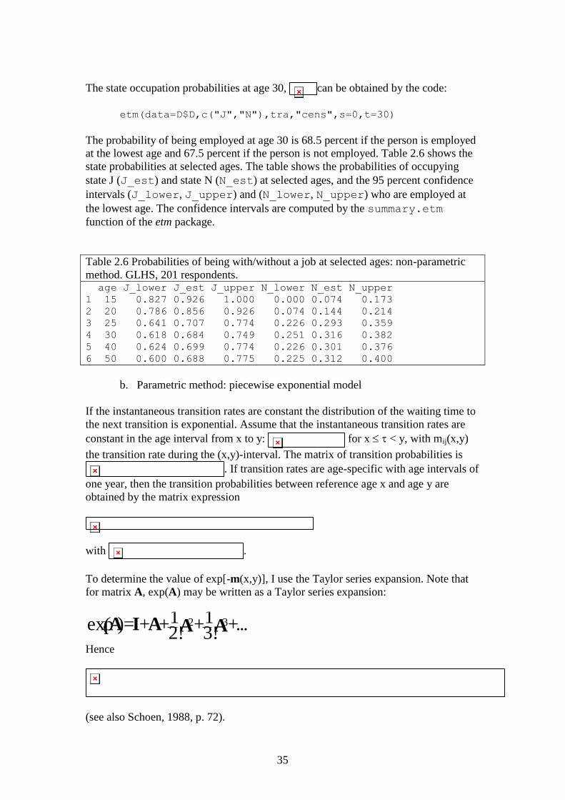
35

The state occupation probabilities at age 30, can be obtained by the code:

etm(data=D$D,c("J","N"),tra,"cens",s=0,t=30)

The probability of being employed at age 30 is 68.5 percent if the person is employed

at the lowest age and 67.5 percent if the person is not employed. Table 2.6 shows the

state probabilities at selected ages. The table shows the probabilities of occupying

state J (J_est) and state N (N_est) at selected ages, and the 95 percent confidence

intervals (J_lower, J_upper) and (N_lower, N_upper) who are employed at

the lowest age. The confidence intervals are computed by the summary.etm

function of the etm package.

Table 2.6 Probabilities of being with/without a job at selected ages: non-parametric

method. GLHS, 201 respondents. age J_lower J_est J_upper N_lower N_est N_upper

1 15 0.827 0.926 1.000 0.000 0.074 0.173

2 20 0.786 0.856 0.926 0.074 0.144 0.214

3 25 0.641 0.707 0.774 0.226 0.293 0.359

4 30 0.618 0.684 0.749 0.251 0.316 0.382

5 40 0.624 0.699 0.774 0.226 0.301 0.376

6 50 0.600 0.688 0.775 0.225 0.312 0.400

b. Parametric method: piecewise exponential model

If the instantaneous transition rates are constant the distribution of the waiting time to

the next transition is exponential. Assume that the instantaneous transition rates are

constant in the age interval from x to y: for x < y, with mij(x,y)

the transition rate during the (x,y)-interval. The matrix of transition probabilities is

. If transition rates are age-specific with age intervals of

one year, then the transition probabilities between reference age x and age y are

obtained by the matrix expression

with .

To determine the value of exp[-m(x,y)], I use the Taylor series expansion. Note that

for matrix A, exp(A) may be written as a Taylor series expansion:

. . . + 3!1 +

2!1 + + = )exp 32 AAAI A(

Hence

(see also Schoen, 1988, p. 72).

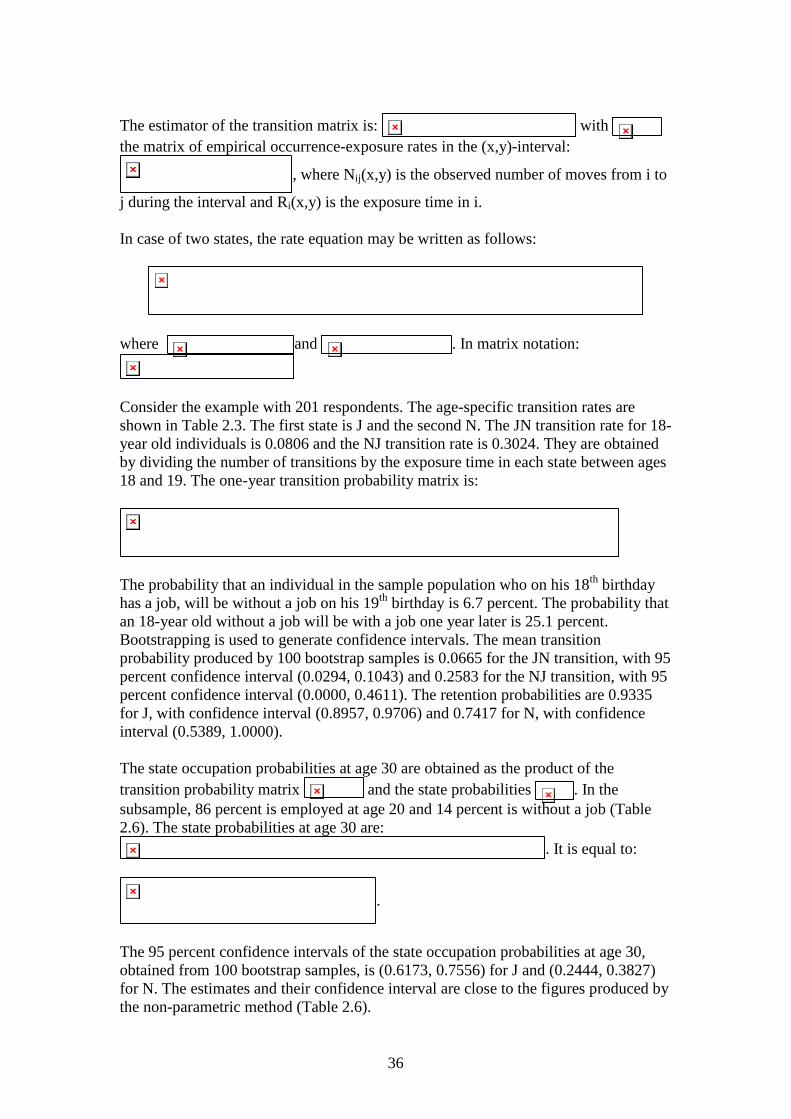
36

The estimator of the transition matrix is: with

the matrix of empirical occurrence-exposure rates in the (x,y)-interval:

, where Nij(x,y) is the observed number of moves from i to

j during the interval and Ri(x,y) is the exposure time in i.

In case of two states, the rate equation may be written as follows:

where and . In matrix notation:

Consider the example with 201 respondents. The age-specific transition rates are

shown in Table 2.3. The first state is J and the second N. The JN transition rate for 18-

year old individuals is 0.0806 and the NJ transition rate is 0.3024. They are obtained

by dividing the number of transitions by the exposure time in each state between ages

18 and 19. The one-year transition probability matrix is:

The probability that an individual in the sample population who on his 18th

birthday

has a job, will be without a job on his 19th

birthday is 6.7 percent. The probability that

an 18-year old without a job will be with a job one year later is 25.1 percent.

Bootstrapping is used to generate confidence intervals. The mean transition

probability produced by 100 bootstrap samples is 0.0665 for the JN transition, with 95

percent confidence interval (0.0294, 0.1043) and 0.2583 for the NJ transition, with 95

percent confidence interval (0.0000, 0.4611). The retention probabilities are 0.9335

for J, with confidence interval (0.8957, 0.9706) and 0.7417 for N, with confidence

interval (0.5389, 1.0000).

The state occupation probabilities at age 30 are obtained as the product of the

transition probability matrix and the state probabilities . In the

subsample, 86 percent is employed at age 20 and 14 percent is without a job (Table

2.6). The state probabilities at age 30 are:

. It is equal to:

.

The 95 percent confidence intervals of the state occupation probabilities at age 30,

obtained from 100 bootstrap samples, is (0.6173, 0.7556) for J and (0.2444, 0.3827)

for N. The estimates and their confidence interval are close to the figures produced by

the non-parametric method (Table 2.6).

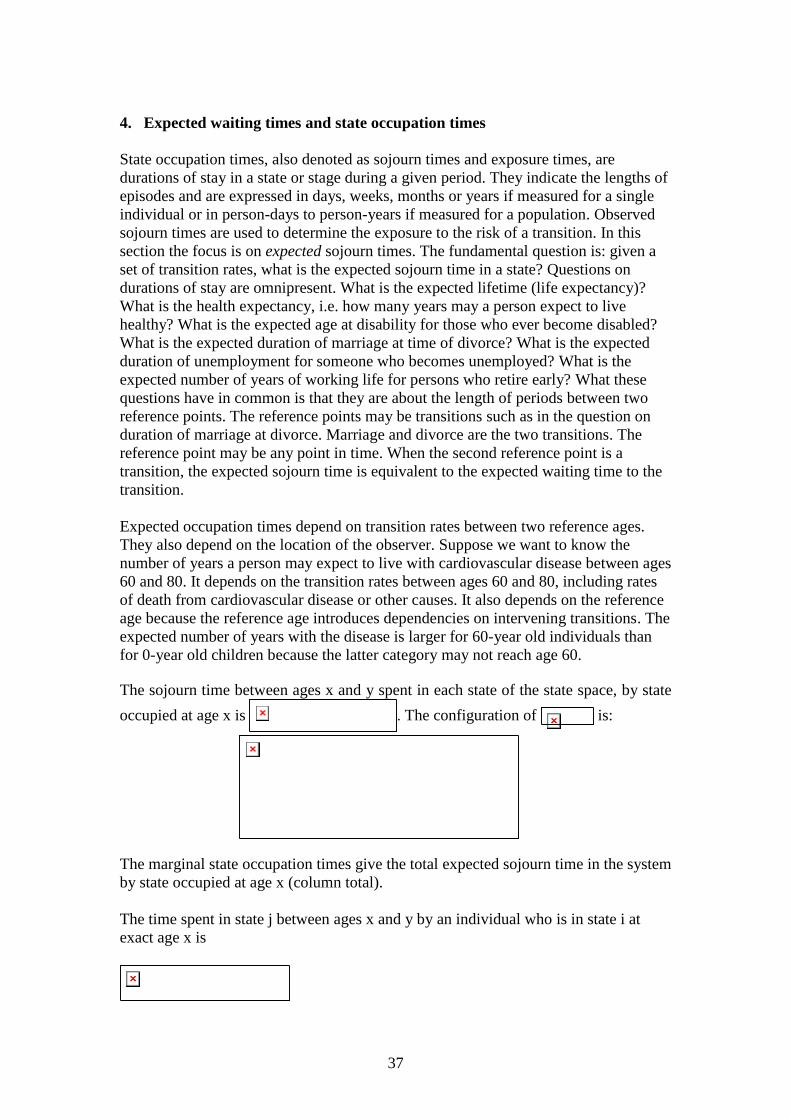
37

4. Expected waiting times and state occupation times

State occupation times, also denoted as sojourn times and exposure times, are

durations of stay in a state or stage during a given period. They indicate the lengths of

episodes and are expressed in days, weeks, months or years if measured for a single

individual or in person-days to person-years if measured for a population. Observed

sojourn times are used to determine the exposure to the risk of a transition. In this

section the focus is on expected sojourn times. The fundamental question is: given a

set of transition rates, what is the expected sojourn time in a state? Questions on

durations of stay are omnipresent. What is the expected lifetime (life expectancy)?

What is the health expectancy, i.e. how many years may a person expect to live

healthy? What is the expected age at disability for those who ever become disabled?

What is the expected duration of marriage at time of divorce? What is the expected

duration of unemployment for someone who becomes unemployed? What is the

expected number of years of working life for persons who retire early? What these

questions have in common is that they are about the length of periods between two

reference points. The reference points may be transitions such as in the question on

duration of marriage at divorce. Marriage and divorce are the two transitions. The

reference point may be any point in time. When the second reference point is a

transition, the expected sojourn time is equivalent to the expected waiting time to the

transition.

Expected occupation times depend on transition rates between two reference ages.

They also depend on the location of the observer. Suppose we want to know the

number of years a person may expect to live with cardiovascular disease between ages

60 and 80. It depends on the transition rates between ages 60 and 80, including rates

of death from cardiovascular disease or other causes. It also depends on the reference

age because the reference age introduces dependencies on intervening transitions. The

expected number of years with the disease is larger for 60-year old individuals than

for 0-year old children because the latter category may not reach age 60.

The sojourn time between ages x and y spent in each state of the state space, by state

occupied at age x is . The configuration of is:

The marginal state occupation times give the total expected sojourn time in the system

by state occupied at age x (column total).

The time spent in state j between ages x and y by an individual who is in state i at

exact age x is

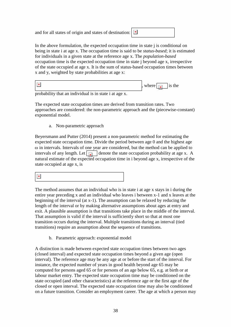
38

and for all states of origin and states of destination:

In the above formulation, the expected occupation time in state j is conditional on

being in state i at age x. The occupation time is said to be status-based; it is estimated

for individuals in a given state at the reference age x. The population-based

occupation time is the expected occupation time in state j beyond age x, irrespective

of the state occupied at age x. It is the sum of status-based occupation times between

x and y, weighted by state probabilities at age x:

, where is the

probability that an individual is in state i at age x.

The expected state occupation times are derived from transition rates. Two

approaches are considered: the non-parametric approach and the (piecewise-constant)

exponential model.

a. Non-parametric approach

Beyersmann and Putter (2014) present a non-parametric method for estimating the

expected state occupation time. Divide the period between age 0 and the highest age

in intervals. Intervals of one year are considered, but the method can be applied to

intervals of any length. Let denote the state occupation probability at age x. A

natural estimate of the expected occupation time in i beyond age x, irrespective of the

state occupied at age x, is

The method assumes that an individual who is in state i at age x stays in i during the

entire year preceding x and an individual who leaves i between x-1 and x leaves at the

beginning of the interval (at x-1). The assumption can be relaxed by reducing the

length of the interval or by making alternative assumptions about ages at entry and

exit. A plausible assumption is that transitions take place in the middle of the interval.

That assumption is valid if the interval is sufficiently short so that at most one

transition occurs during the interval. Multiple transitions during an interval (tied

transitions) require an assumption about the sequence of transitions.

b. Parametric approach: exponential model

A distinction is made between expected state occupation times between two ages

(closed interval) and expected state occupation times beyond a given age (open

interval). The reference age may be any age at or before the start of the interval. For

instance, the expected number of years in good health beyond age 65 may be

computed for persons aged 65 or for persons of an age below 65, e.g. at birth or at

labour market entry. The expected state occupation time may be conditioned on the

state occupied (and other characteristics) at the reference age or the first age of the

closed or open interval. The expected state occupation time may also be conditioned

on a future transition. Consider an employment career. The age at which a person may

39

experience a first episode without work after a period with employment is lower for

those who will ever experience an episode without work than for the average

population. The expected occupation time during an age interval, conditioned on a

transition occurring with certainty during that interval, is less than the expected

occupation time that is not conditioned on a transition occurring. For instance, the

expected duration of marriage at divorce is lower for those who ever divorce than for

the average married population. The latter includes those who never divorce.

The time spent in state j between ages x and y by an individual who is in state i at

exact age x is , where an element denotes the time

an individual in i at age x may expect to spend in j between ages x and y. If the

transition rates are constant in the (x,y)-age interval (exponential model), the

integration of the equation leads to:

,

which is equal to:

,

provided m(x,y) is not singular. The expression is also shown by Namboodiri and

Suchindran (1987, p. 145), Schoen (1988, p. 101) and van Imhoff (1990). If m(x,y) is

singular, a very small value may be added to the diagonal elements of the matrix.

Izmirlian et al. (2000, p. 246), who consider the case with an absorbing state (death),

suggest to replace by one the zero diagonal element corresponding to the absorbing

state. I choose to add a small value (10-8

) to the diagonal. It may be viewed as a rate

of a fictitious attrition. It is too small to occur between x and y but it is large enough

to make m(x,y) non-singular.

Taylor series expansion of results in the following equivalent

expression for the state occupation times (Schoen, 1988, p. 73):

When the interval is short, the sojourn time may be approximated by the linear

integration hypothesis, which implies the assumption of uniform distribution of events

(linear model):

),(2

),(x yxxyyx PIL

The linear method is usually used in demography and actuarial science. It is often

referred to as the actuarial method.

40

The reference age may be any age at or before the start of the interval. Consider the

reference age zero. The expected time newborns may expect to spend in each state

between ages x and y, by state at birth, is

where P(0,x) represents the transition probabilities between ages 0 and x. When the

reference age changes from age 0 to age x, the expected length of stay in the various

states between ages x and y changes from an unconditional measure to a conditional

measure. It becomes conditional on being present in the population at x. The measure

is

,

provided the inverse of P(0,x) exists. The state occupation times between ages x and

y, a new-born may expect, irrespective of the state occupied at birth is .

The estimation of the expected state occupation times beyond a given age requires the

state occupation time beyond the highest age group. If at high ages few transitions

occur, the ages are often collapsed in an open-ended age group with constant

transition rates. Demographers use that approach to close the life table. Let z denote

the first age of the highest open-ended age group. The sojourn time in the various

states beyond age z by individuals present at z is

, where denotes infinity.

The life expectancy at age x is the number of years an individual aged x may expect

to spend in each state beyond age x, by state occupied at x or irrespective of the state

occupied at x. It is . An element of is the

number of years an individual who is in state i at age x may expect to spend in state j

beyond age x. is a matrix with the state at age x as the column variable and

the state occupied beyond age x the row variable. It gives the expected remaining

lifetime conditional on the state occupied at age x. In multistate demography, it is

known as the status-based life expectancy at age x. The population-based life

expectancy is the time an individual aged x may expect to spend in each of the states

beyond age x, irrespective of the state occupied at age x. It is multiplied by

the vector of state occupation probabilities at age x.

If transition rates are age-specific, i.e. piecewise-constant, and the length of an age

interval is one year, then the expected state occupation times at reference age x is

with and .

The expected occupation time in state i depends on the rate of leaving i. If the exit

rate between ages x and y is zero, an individual in i at age x will remain in i at least

41

until age y. If a departure from i occurs during the (x,y)- interval, it will occur at an

occupation time which is less than the expected occupation time. In other words, the

expected occupation time, conditioned on a transition occurring, is less than the

expected occupation time that is not conditioned on a transition occurring. Consider

an individual in state i at age x. The expected waiting time to leaving i between x and

y consists of two parts. The first is the state occupation time for stayers. It is equal to

y – x. The probability of staying in i during the entire interval from x to y is the

survival probability . The second part is the waiting time

to an exit from i that occurs before y. It is denoted by . Hence the occupation

time equation is and

. It is the time an individual aged x in i spends

in i on a continuous basis before leaving, provided the exit occurs before y. The

occupation time equation distinguishes stayers and leavers.

The fraction of an interval spent in a given state if a transition occurs with certainty is

frequently referred to as Chiang’s “a”, after the statistician Chiang who introduced it.

Chiang, who developed the measure in the context of mortality, called “a” the fraction

of the last year of life (Chiang, 1968, pp 190ff; 1984, pp. 142ff). Schoen (1988, p. 8

and p. 71) uses the concept of mean duration at transfer to denote the expected

number of years before the transition. It is the product of Chiang’s “a” (fraction of the

interval) and the length of the interval. If transitions are uniformly distributed during

the interval, the survival function is linear and “a” is half the length of the interval. If

the transition rate is constant during an interval, the waiting time to the event is

exponentially distributed. Consequently, the expected time to an event that occurs

with certainty is less than half the interval length. The probability that an exit from

state i during the (x,y)-interval occurs during the first half of the interval, provided it

occurs with certainty during the interval, is a ratio of two distribution functions:

.

Consider the 201 respondents and age 18. The expected occupation times in each of

the states of the state space (J and N) by state on the 18th

birthday is

A person of exact age 18 with employment may expect to spend 0.036 years (less

than half a month) without employment before reaching age 19. The 95 percent

confidence interval, produced by bootstrapping, is (0.0136, 0.0635). A person of the

same age without a job may expect to be employed during 0.134 years (1.6 months)

before his 19th

birthday, with confidence interval (0.0323, 0.2663). A small figure (10-

8) has been added to the diagonal to prevent m(18,19) from being singular. A person

aged 18 with employment, who leaves employment before age 19, may expect to

leave employment after years or 5.6 months. The Taylor

42

series expansion gives about the same result. A sum of four terms plus the identity

matrix gives .

The number of years between the lowest age (14) and the highest age (54) is 40 years.

Since states J and N are transient states, the total numbers of years spent in the

employment career between ages 14 and 54 is 40. If a hypothetical individual starts at

age 14 with a job and the employment career is governed by the occurrence-exposure

rates estimated from the GLHS subsample of 201 subjects, then the expected number

of years with a job is 28.66 and the number of years without a job is 11.34. The

average of the 100 bootstrap samples is 28.55 and 11.45, respectively. The 95 percent

confidence intervals are (26.65, 30.28) and (9.72, 13.35).

5. Synthetic life histories

The methods presented in the previous sections produce state probabilities and

expected occupation times that are consistent with empirical transition rates. The state

probabilities and the occupation times describe the expected life history, given the

data. The confidence intervals around the expected values indicate the degree of

uncertainty in the data. Transition rates are differentiated by age to capture the age

patterns of transitions. In this section, age-specific transition rates are considered,

with age intervals of one year. Transition rates are piecewise constant: they vary

between age groups but they are constant within age groups. Individual life histories

differ from the expected life history because of observed differences between

individuals with different personal attributes, unobserved differences and chance. The

chance mechanism is the subject of this section. Observed and unobserved differences

are disregarded because they are beyond the scope of this chapter. Synthetic

individual life histories are generated using longitudinal microsimulation (Willekens,

2009; Zinn, 2011; Zinn et al., 2013; Zinn, 2014). The method is consistent with

Discrete Event Simulation (DEV) methods.

To explain the chance mechanism, a single transition rate will do and to explain the

basic principle of generating synthetic biographies, a single transition rate matrix is

sufficient. To generate more realistic synthetic biographies, age-specific transition

rates are used. Consider the 201 respondents of the GLHS sample and the observation

period between labour market entry and survey date. In Section 2.2, the aggregate NJ

transition rate was estimated at 0.096 per year (using msm). An individual who

previously had a job (the nature of the sample) and who is currently without a job,

may expect to get another job in 10.4 years (1/0.096) on average. The expected

waiting time during the first year is years. It is high

because at the time the data were collected a relatively large number of respondents,

in particular women, left the labour force and did not return. The probability of

experiencing the event in the first year is 9.154 percent [100*(1-exp(-0.096))]. An

individual without a job, who gets a job within one year, waits 0.4920 years, on

average. This is a little less than 6 months. Individual waiting times are random

variables; the values are distributed around these expected value. Since the transition

rate is constant at 0.096, individual waiting times are exponentially distributed with a

mean of 10.4 years and a variance of 108 years, assuming no competing transition

43

intervenes in the labour market transitions. The median waiting time is 7.2 years

[ln(2)]/0.096.

To obtain individual waiting times that are consistent with these expected values,

waiting times are drawn randomly from an exponential distribution with a hazard rate

0.096 or, alternatively, a mean waiting time of 10.4 years. A random draw is

implemented in two steps. First, a random number is drawn from the standard uniform

continuous distribution U[0,1]. Every value between zero and one is equally likely to

occur. The random number drawn represents the probability that the waiting time to

the transition is less then or equal to t, where t needs to be determined. Let denote

the probability. Hence: . Suppose =0.54. The value of t is

derived from the inverse distribution function of the exponential distribution. It is

years. N draws from the uniform distribution

result in N individual waiting times. If N is sufficiently large, the sample mean is

close to the expected value of 10.4 years and the sample variance is close to 108

years. One experiment of 1000 draws resulted in a mean waiting time of 10.11 years

and a variance of 116.5 years. Another experiment resulted in a mean waiting time of

9.89 years and a variance of 87.4 years.

The transition rate estimated from data, in this example 0.096, is subject to sample

variation. The rate is itself a random variable. If the number of observations is

sufficiently large, the rate is a normally distributed random variable with the expected

value as its mean. The 95 percent confidence interval of the NJ transition rate was

estimated at (0.0804, 0.1146). To incorporate the degree of uncertainty in the data in

the generation of synthetic life histories, a transition rate may be drawn from a normal

distribution with mean ln(0.096) and standard deviation . The

standard deviation of the NJ transition rate was computed in Section 2.2 of this

chapter. If the value drawn from a normal distribution is denoted by m, then the

transition rate is exp(m). An alternative to drawing a transition rate from a normal

distribution is to resample the data (with replacement) and to estimate the transition

rate from the new sample. In this approach, the distribution of the transition rate is the

distribution generated by bootstrap samples. Consider 100 bootstrap samples and 100

transition rates, one from each sample. Each of these transition rates is used to

generate 1000 individual waiting times. The collection of waiting time incorporates

the effects of sample variation and the exponential distribution of waiting times. For a

person without a job, the overall average waiting time to a job is 10.54 years and the

variance is 115.00 years. The NJ transition rates estimated in the bootstrap samples

vary from 0.073 to 0.140, with mean rate 0.0967.

The aggregate transition rates may be used to generate employment histories. The JN

transition rate is 0.0533 and the NJ transition rate is 0.0960. Recall that observations

started at labour market entry (first job). Hence N refers to being without a job, after

having had at least one job. The transition rate matrix is .

Everyone starts the employment history in J. The starting time is zero, meaning that

the time is measured as time elapsed since labour market entry. The employment

history is simulated for 30 years (simulation stop time). The transition rates are

44

assumed to remain constant during that period. In this example, employment histories

are sequences of transitions and waiting times to transitions. They are assumed to be

outcomes of a continuous-time Markov model with constant rates. The simulation

runs as follows. Let t denote time. An individual starts in J at time 0. A random

number is drawn from an exponential distribution with transition rate 0.0533 to

determine the time to transition from J to N. One draw results in a transition at t=8.29

years. To determine how long the individual stays in N, a random number is drawn

from an exponential distribution with transition rate 0.096. The randomly selected

time to NJ transition is 4.30 years. Hence the individual starts a second job 12.59

years after labour market entry (8.29+4.30). A new random waiting time is drawn

from an exponential distribution with transition rate 0.0533 to determine the time of

the second JN transition. The number is 24.00, which means that the transition would

occur 36.59 years after labour market entry. The transition time exceeds the time

horizon of 30 years and is not considered. When the simulation is discontinued, the

individual is in state J. The function sim.msm of the msm package is used to

generate the life history of a single individual. The code is:

m <- array(c(0.0533,-0.0533,-0.096,0.096),

dim=c(2,2),dimnames=list(destination=c("J","N"),

origin=c("J","N")))

bio <- sim.msm (-t(m),mintime=0,maxtime=30,start=1)

where m is the transition rate matrix shown above, mintime is the starting time of

the simulation, maxtime is the ending time and start is the starting state (J is state

1 and N is state 2). The object bio has two components. The first contains the state

sequence and the second the transition times.

The distribution of employment histories that are consistent with the transition rates

may be obtained by simulating a large number of employment histories. In this simple

illustration, the transition rates are assumed not to depend on age and to remain

constant during the period of 30 years. Simulation of 1,000 employment histories

results in the distribution shown in Table 2.7. The most frequent trajectory is JNJ,

about one third of all trajectories. The trajectories JN and J cover about one fifth each.

These 3 trajectories account for 68 percent of all trajectories during a period of 30

years. For each trajectory, the median ages at transition are also shown. The table is

produced by the Sequences function of Biograph. The results of the simulation are

stored in a Biograph object, which facilitates analysis of the simulated life histories.

Table 2.7 Employment histories in virtual population, based on GLHS aggregate

transition rates. ncase % cum% path tr1 tr2 tr3 tr4

1 305 30.5 30.0 JNJ 9.12>N 19.95>J

2 194 19.4 49.9 JN 20.35>N

3 185 18.5 68.4 J

4 130 13.0 81.4 JNJNJ 4.81>N 10.42>J 18.86>N 24.91>J

5 121 12.1 93.5 JNJN 6.53>N 13.28>J 25.83>N

Constant transition rates have been used for illustrative purposes only. Usually, age-

specific transition rates are used to generate synthetic life histories. Suppose an

individual enters his first job at age 21.3 (decimal year). He experiences the

employment exit rate from age 21.3 onwards until (a) he enters a period without a job,

45

(b) he experiences a competing transition, or (c) the ‘observation’ is censored, i.e.

simulation is discontinued. In this illustration, no competing transition is considered.

Hence the waiting time to the JN transition depends on the age-specific transition

rates between age 21.3 and the age at which simulation is discontinued, which in the

sample of 201 respondents is 52. Age-specific transition rates are weighted by

exposure time. The transition rate at age 21 is multiplied by the duration of exposure,

which is 0.7 years (22.0 – 21.3). The transition rates at age 22 and higher are

multiplied by one. The sum of the age-specific transition rates beyond age 21 is the

cumulative transition rate, computed at age 21. The waiting time to the JN transition

is determined by a random draw from an exponential waiting time distribution

associated with the cumulative transition rate computed at age at labour market entry.

The age at the JN transition is the current age plus the waiting time to the JN

transition. Suppose a waiting time of 3.4 years is drawn. The individual will enter a

period without a job at age 24.4. If the waiting time is such that the age at transition

exceeds the highest age in the observation scheme, then the observation is censored at

the highest age.

If the number of states exceeds two, the destination state must be determined in

addition to the time to transition. A multinomial distribution is used. The distribution

is derived from the origin-destination specific transition rates. If mij(x,y) is the (i,j)-

transition rate between ages x and y, then the probability of selecting state j,

conditional on leaving i, is: , with . The

probability is an event probability, not a transition probability. The probabilities are

used to partition the interval between the minimum probability (0) and the maximum

probability (1): . A random number is drawn

from a standard uniform distribution and the interval that corresponds to its value

determines the destination state. The method is implemented in the msm package.

The method of estimating time to transition and destination state consists of two steps.

The first uses the exit rate from the current state, i say, to determine the time to

transition (exit from i). The exit rate is taken from the diagonal of the transition rate

matrix. The second step is to determine the destination, conditional on leaving the

current state. This method was suggested by Wolf (1986). An alternative but

equivalent method relies on the destination-specific transition rates. Consider an

individual in state i at age x. For each possible destination j random waiting times are

drawn from exponential distributions with parameters the cumulative (i,j)-transition

rates between x and the highest age: . If transition rates are

piecewise constant (age-specific), the cumulative hazard is piecewise linear. The

smallest random waiting time determines the destination. The two methods rely on the

theory of competing risks and assume that the waiting times corresponding to the

distinct destinations are independent. Zinn (2011, pp. 177ff) shows that the two

methods give similar results. Notice that the two methods are also consistent with

discrete event simulation (DEVS), although only the second method stores randomly

drawn waiting times in event queues before selecting the shortest waiting time. The

LifePaths (Statistics Canada2) and MicMac microsimulation models (Gampe and

2 http://www.statcan.gc.ca/microsimulation/lifepaths/lifepaths-eng.htm

46

Zinn, 2008) use event queues. The msm package uses exit rates and conditional

destination probabilities.

For illustrative purposes, the transition rates in Table 2.3, are used to generate

synthetic employment histories for 2010 individuals, 10 for each observation in the

GLHS subsample of 201 respondents. For each individual in the GLHS sample, 10

employment histories are simulated to reduce the Monte Carlo variation. The

employment career is simulated between a low age and a high age. The ages are

determined by individual observation periods in the GLHS subsample of 201

respondents. For instance, individual 1 enters the labour market at age 17 and is 52 at

interview. In the virtual population, 10 individuals enter the labour market at age 17

and are interviewed at age 52. Individual 4 is 22 at labour market entry and 31 at

interview. The ages of labour market entry and interview of that respondent are

imposed on 10 individuals in the virtual population. The simulated employment

histories cover the same age intervals as the observed employment histories.

Differences between simulated and observed employment trajectories are due to

sample variation affecting the estimated transition rates and Monte Carlo variation in

the simulation. Table 2.8 shows the main employment trajectories in the observed and

the simulated population. For a given trajectory, the number of simulated trajectories

should be about 10 times the observed trajectories because 10 simulations were

performed for each observation. The table also shows the median ages at transition.

The results differ considerably because in the GLHS, which was organized in 1981,

women and men report very different employment histories and the transition rates

are not differentiated by sex. If the transitions rates are estimated separately for males

and females, and employment trajectories are produced for the two sexes separately,

the simulated trajectories are much closer to the observations (Table 2.8). Among

females, JN is the most frequent trajectory, whereas it is quite rare among males. For

both men and women the model accurately estimates the proportion of persons

employed continuously throughout the observation period. For women, it

underestimates permanent withdrawal from the labour market after a single

employment episode and overestimates re-entry. That may be due to a cohort effect

with younger cohorts more likely to re-enter the job market after a period of absence.

The sample size is too small to estimate age-specific transition rates by sex and birth

cohort.

Table 2.8 Employment histories in observed population and virtual population, based on

age-specific GLHS transition rates. A. Observed trajectories: males and females combined

ncase % cum% case tr1 tr2 tr3 tr4

1 67 33.33 33.33 J

2 54 26.87 60.20 JNJ 21.71>N 26.17>J

3 44 21.89 82.09 JN 24.88>N

4 16 7.96 90.05 JNJNJ 20.83>N 23.96>J 25.62>N 29.62>J

5 10 4.98 95.02 JNJN 20.12>N 21.21>J 29.62>N

B. Simulated trajectories: males and females combined

ncase % cum% case tr1 tr2 tr3 tr4

1 627 31.19 31.19 J

2 531 26.42 57.61 JNJ 22.99>N 27.33>J

3 294 14.63 72.24 JN 27.2>N

4 245 12.19 84.43 JNJN 21.21>N 24.3>J 30.31>N

5 218 10.85 95.27 NJNJ 20.66>N 22.31>J 26.92>N 32.43>J

C. Observed trajectories: males

ncase % cum% case tr1 tr2 tr3 tr4 tr5 tr6

47

1 52 49.06 49.06 J

2 41 38.68 87.74 JNJ 21.92>N 25.33>J

3 6 5.66 93.40 JNJNJ 18.42>N 20.17>J 22.71>N 24.04>J

4 3 2.83 96.23 JN 27.5>N

5 3 2.83 99.06 JNJNJNJ 18.17>N 19.67>J 21.5>N 22.08>J 33.17>N 35.75>J

D. Simulated trajectories: males

ncase % cum% case tr1 tr2 tr3 tr4 tr5 tr6

1 518 48.87 48.87 J

2 314 29.62 78.49 JNJ 21.5>N 24.93>J

3 131 12.36 90.85 JNJNJ 20.54>N 22.54>J 26.81>N 28.85>J

4 35 3.30 94.15 JNJN 21.3>N 23.37>J 34.4>N

5 23 2.17 96.32 JNJNJNJ 20.4>N 21.65>J 22.52>N 23.85>J 28.4>N 30.62>J

E. Observed trajectories: females

ncase % cum% case tr1 tr2 tr3 tr4 tr5 tr6

1 41 43.16 43.16 JN 24.67>N

2 15 15.79 58.95 J

3 13 13.68 72.63 JNJ 21.5>N 29.58>J

4 10 10.53 83.16 JNJN 20.12>N 21.21>J 29.62>N

5 10 10.53 93.68 JNJNJ 23.21>N 26.29>J 27.62>N 32.25>J

6 5 5.26 98.95 JNJNJN 18.5>N 19.67>J 27.17>N 28.42>J 32.58>N

7 1 1.05 100.00 JNJNJNJ 21.92>N 22.08>J 33.83>N 35.08>J 39.83>N 40.17>J

F. Simulated trajectories: females

ncase % cum% case tr1 tr2 tr3 tr4

1 337 35.47 35.47 JN 25.32>N

2 183 19.26 54.74 JNJN 21.13>N 25.5>J 30.11>N

3 174 18.32 73.05 JNJ 24.43>N 31.99>J

4 139 14.63 87.68 J

5 62 6.53 94.21 JNJNJ 20.91>N 24.31>J 28.8>N 37.05>J

6. Conclusion

Life histories are operationalised as state and event sequences. Synthetic life histories

describe sequences that would result if individual life courses are governed by

transition rates estimated from life history data. Transition rates link real and synthetic

life histories. If transition rates are accurate, synthetic biographies mimic observed

life paths. Life history data are generally incomplete. They do not cover the entire life

span. By combining data from similar individuals, the transition rates may cover the

entire life span. The estimation of transition rates is crucial. In this chapter, two

estimation methods are described. The first is non-parametric and the second is

parametric, or more appropriate, partial parametric. The non-parametric approach is

common in biostatistics. The Nelson-Aalen estimator of transition rates is

distribution-free, it does not rely on an assumption that the data are drawn from an

underlying probability distribution. The partial parametric method is common in

demography, epidemiology and actuarial science. The occurrence-exposure rate

computed for an age interval assumes that the transition rate is constant within the

interval. Occurrence-exposure rates vary freely between intervals. The two methods

converge when the interval gets infinitesimally small.

Transition rates are used to generate synthetic biographies. Synthetic biographies

describe life histories in terms of state occupation probabilities and expected state

occupation times. Life expectancies, healthy life expectancies and active life

expectancies are examples of state occupation times. Life histories generated by the

most likely transition rates, given the data, are expected life histories. They apply to a

population. Few individuals have a life path that coincides with the expected life

history. Microsimulation is used to determine the distribution of individual life

48

histories around expected life histories. The method presented in this chapter involves

drawing individual waiting times to transitions from piecewise-exponential waiting

time distributions. Sequences of waiting times are obtained by joining randomly

drawn waiting times. The method, which is referred to as longitudinal

microsimulation, is described in the chapter. The added value of synthetic individual

life paths is the information they provide on the distribution of (1) state and event

sequences and (2) state occupation times around expected values. Synthetic individual

biographies describe life paths in a virtual population. The virtual population closely

resembles the real population if (1) transition rates are accurately estimated and (2)

the observation plan applied to the real population is also applied to the virtual

population, i.e. simulated life segments fully coincide with observed life segments.

The variation of individual life histories indicates uncertainties in the data and

uncertainties associated with drawing random numbers from probability distributions.

The uncertainties translate into uncertainties in transition rates, transition and state

probabilities and expected state occupation times. Uncertainties in transition rates can

be measured assuming that transition rates or transformations of transition rates are

normally distributed (asymptotic theory). The distributions of probabilities and

occupation times are more complicated and cannot always be expressed analytically.

In the chapter, bootstrapping is used to estimate the uncertainties in transition

probabilities, state probabilities and occupation times. If the cohort biography

(expected life path) is computed for each bootstrap sample, the distribution of cohort

biographies can be determined. By combining bootstrapping and longitudinal

microsimulation, synthetic individual biographies can be produced that incorporate

uncertainties in the data and uncertainties introduced by the microsimulation (Monte

Carlo variation). The latter results from drawing random numbers from probability

distributions. The precision of the method of computing synthetic biographies from

real data is measured by comparing summary statistics of virtual and real populations.

The methods described in this chapter are implemented in Biograph and other

packages discussed in this book. The packages have in common that they adopt a

counting process point of view (Aalen et al., 2008).

49

References

Aalen, O.O., Ø. Borgan and H.K. Gjessing (2008) Survival and event history analysis.

A process point of view. Springer, New York.

Allignol, A. (2012a) The mvna package. Nelson-Aalen estimator of the cumulative

hazard in multistate models. Available at

http://cran.r-project.org/web/packages/mvna/index.html

Allignol, A. (2012b) Package etm. Empirical transition matrix. Available at

http://cran.r-project.org/web/packages/etm/index.html

Allignol, A., J. Beyersmann and M. Schumacher (2008) mvna: An R package for the

Nelson-Aalen estimator in multistate models. R Newsletter, 8(2):48-50

Allignol, A., M. Schumacher and J. Beyersmann (2011) Empirical transition matrix of

multistate models: the etm package. Journal of Statistical Software, 38(4), 15 pp.

Andersen, P.K. and N. Keiding (2002) Multi-state models for event history analysis.

Statistical Methods in Medical Research, 11:91-115.

Aoki, M. (1996) New approaches to macroeconomic modeling. Evolutionary

stochastic dynamics, multiple equilibria, and externatities as field effects. Cambridge

University press, Cambridge, UK.

Beyersmann, J. and H. Putter (2011) A brief note on computing average state

occupation times. Memo.

Beyersmann, J., M. Schumacher and A. Allignol (2012) Competing risks and

multistate models with R. Springer, New York.

Blossfeld, H.P. and G. Rohwer (2002) Techniques of event history modeling. New

approaches to causal analysis. Lawrence Erlbaum, Mahwah, New Jersey (2nd

Edition).

Chiang. C.L. (1968) Introduction to stochastic processes in biostatistics. Wiley, New

York. Chapter 9 reprinted in D.J. Bogue, E.E. Arriage and E.L. Anderton eds. (1993)

Readings in population research methodology. Vol 2, pp. 7.84-7.97.

Chiang, C.L. (1984) The life table and its applications. R.E. Krieger Publishing,

Malabar, Fl.

Çinlar, E. (1975) Introduction to stochastic processes. Prentice-Hall, Englewood

Cliffs, New Jersey.

De Wreede, L.C., M. Fiocco and H. Putter (2010) The mstate package for estimation

and prediction in non- and semi-parametric multi-state and competing risks models.

Computer Methods and Programs in Biomedicine, doi:10.1016/j.cmpb.2010.01.001

50

De Wreede, L.C., M. Fiocco and H. Putter (2011) mstate: An R package for the

analysis of competing risks and multistate models. . Journal of Statistical Software,

38(7).

Helbing. D. (2010) Quantitative Sociodynamics. Stochastic Methods and Models of

Social Interaction Processes. Springer, Berlin.

Hoem, J.M. and U. Funck Jensen (1982) Multistate life table methodology: a

probabilist critique. In: K.C. Land and A. Rogers eds. Multidimensional mathematical

demography. Academic Press, New York, pp. 155-264.

Holford, T.R. (1980) The analysis of rates and of survivorship using log-linear

models. Biometrics, 36:299-305.

Hougaard, P. (2000) Analysis of multistate survival data. Springer, New York.

Izmirlian, G., D. Brock, L. Ferrucci and C. Phillips (2000) Active life expectancy

from annual follow-up data with missing responses. Biometrics, 56(1):244-248.

Jackson, C. (2012) The msm package.

http://cran.fiocruz.br/web/packages/msm/msm.pdf

Jackson, C. (2011) Multi-state models for panel data: the msm package for R. Journal

of Statistical Software, 38(8), 28 pp.

Kalbleisch J.D. and R.L. Prentice (2002) The statistical analysis of failure time data.

Wiley, New York. Second edition.

Korn, E.I., B.I. Graubard and D. Midthune (1997) Time-to-event analysis of

longitudinal follow-up of a survey: choice of time-scale. American Journal of

Epidemiology, 145(1):72-80.

Laird, N. and D. Olivier (1981) Covariance analysis of censored survival data using

log-linear analysis techniques. Journal of the American Statistical Association,

76(374): 231-240.

Li, Y., M.H. Gail, D.L. Preston, B.I. Graubard and J.H Lubin (2012) Piecewise

exponential survival times and analysis of case-control data. Statistics in Medicine,

31(13):1361-1368.

Mamun, A.A. (2003), Life history of cardiovascular disease and its risk factors.

Rozenberg Publishers, Amsterdam.

Meira-Machado, L.M.et al (2009) Multi-state models for the analysis of time-to-

event data. Statistical Methods in Medical Research, 18(2):195-222

Namboodiri, K. and C.M. Suchindran (1987) Life table techniques and their

applications. Academic Press, Orlando.

51

Pencina M.J., M.G. Larson and R.B. D’Agostino (2007) Choice of time scale and its

effect on significance of predictors in longitudinal studies. Statistics in Medicine,

26:1343–59.

Putter, H. (2012) Package dynpred. CRAN repository.

Putter, H., L. de Wreede and M. Fiocco (2012) Package ‘mstate’. CRAN repository.

Reuser, M. (2010) The effect of risk factors on compression or expansion of disability

A Multistate analysis of the U.S. Health and Retirement Study. Rozenberg Publishers,

Amsterdam.

Rogers, A. (1975) Introduction to multiregional mathematical demography. Wiley,

New York.

Rogers, A. (1986) Parameterized multistate population dynamics and projections.

Journal of the American Statistical Association, 81(393):48-61

Schoen, R. (1988) Modeling multigroup populations. Plenum Press, New York.

Tuma, N.B. and M.T. Hannan (1984) Social dynamics. Models and methods.

Academic Press, Orlando, Florida.

Van den Hout, A. (2012) ELECT: Estimation of life expectancies using continuous-

time multi-state suvival models. Available at

http://www.ucl.ac.uk/~ucakadl/ELECT_Manual.pdf

Van den Hout, A. and E.F. Matthews (2008). Multi-state analysis of cognitive ability

data: a piecewise-constant model and a Weibull model. Statistics in Medicine 27:

5440–5455.

Van den Hout, A., E. Ogurtsova, J. Gampe and F.E. Matthews (fortcoming)

Investigating healthy life expectancy using a multi-state model in the presence of

miussing data and misclassification.

Van Houwelingen H.C. and H. Putter (2008) Dynamic predicting by landmarking as

an alternative for multi-state modeling: an application to acute lymphoid leukemia

data. Lifetime Data Analysis 14:447–463.

Van Houwelingen, H.C. and H. Putter (2011) Dynamic prediction in clinical survival

analysis. Chapman and Hall/CRC Press.

Van Imhoff, E. (1990) The exponential multidimensional demographic projection

model. Mathematical Population Studies, 2(3):171-182

Weidlich, W. and G. Haag (1983) Concepts and models of quantitative sociology: the

dynamics of interacting populations. Springer, Berlin.

52

Willekens, F.J. (1987) The marital status life-table. In: J. Bongaarts, T. Burch and

K.W. Wachter eds. Family demography: models and applications. Oxford: Clarendon

Press, pp. 125-149.

Willekens, F.J. (2009) Continuous-time microsimulation in longitudinal analysis. In:

A. Zaidi, A. Harding and P. Williamson eds. New frontiers in microsimulation

modelling. Ashgate, Surrey, UK, pp. 413-436.

Wolf, D.A. (1986) Simulation methods for analyzing continuous-time event history

models. Sociological Methodology, 16:283-308.

de Wreede, L., M. Fiocco and H. Putter (2011) mstate: An R package for the

analysis of competing risks and multi-state models, Journal of Statistical

Software, 38(7).

Zinn, S, (2011) A continuous-time microsimulation and first steps towards a multi-

level approach in demography. PhD dissertation, University of Rostock, Faculty of

Informatics and Electrotechnics.