Preface This ecological handbook (Part II in a series of handbooks for students in marine

sciences) was developed in the framework of the Belgian-Russian collaboration

project ‘Joint Curriculum Development in Geo-Ecological Surveying in areas of

development of Natural resources’. Part I, a geological handbook, has been written in

2000 and is entitled “Gas and fluids in marine sediments and related phenomena”.

The geological handbook contains a series of exercises on the interpretation of

stratigraphy, high-resolution seismics and side-scan sonar of gas hydrates and mud

volcanoes.

The purpose of the present ecological handbook is:

q To give graduate and undergraduate students the opportunity to put their

theoretical knowledge about ecological principles into practice

q To get acquainted with the ecosystems formed by cold-water corals

This handbook is mainly based on material from Lophelia reefs because they are

very diverse, concerning both faunal and structural diversity. Moreover, deep-water

corals form a very interesting and extremely beautiful deep-sea habitat, which makes

them very suitable for educational purposes.

The handbook provides an introduction to cold-water coral ecosystems and

ecological sampling techniques. Frequently used methods in the study of biodiversity

and community structure are briefly introduced and clarified with examples. Then the

user can apply these methods in the exercises at the end of each chapter. All the

exercises are based on photographs and video footage collected in cold-water coral

reefs off Norway and Ireland:

q The Norwegian oil company STATOIL provided a 56 min. long video film of

the Haltenpipe coral reef, reef A (see Hovland & Mortensen, 1999). The video

footage was recorded with the ROV “Solo” in the summer of 1997 at a depth

of 275-320 m. They reveal a Lophelia reef of 100 m in diameter and 31 m

high, and a large variety of associated megafauna. STATOIL also provided 80

digital stereo photographs from the HDP-reef cluster taken in 1993 and 1997.

q IFREMER, the French Institute for Exploitation of the Sea, provided digital

photographs of Lophelia and its associated fauna on Theresa Mound, Ireland.

These pictures were taken during the CARACOLE cruise with the research

ship L’ Atalante in the summer of 2001 (30 Juli-15 August) using the deep-

water remotely operated vehicle (ROV) Victor 6000 to study coral

occurrences in the Porcupine Seabight, the Porcupine Bank and the Rockall

Trough.

Figure 0.1 Maps showing the origin of the visual material used in this handbook. The left map shows cold-water coral sites (black dots) around the British Isles. The material from IFREMER comes from Theresa Mound, which is a part of the ‘Belgica' mound province on the eastern slope of Porcupine Basin. The map on the right shows the coast of Norway with the Sula Ridge indicated by the yellow square. The STATOIL material was collected on the Haltenpipe-reefs, south of the Sula Ridge.

Porcupine

List of contents

1. Introduction

1.1 Deep-water corals

1.2 Distribution of Lophelia pertusa

1.2.1 Substrate

1.2.2 Water-masses, currents and their influence on food-availability

1.2.3 Seepage of hydrocarbons

1.3 Lophelia and human activities

2. Material and Methods

2.1 Locating and Mapping

2.2 Sampling

2.2.1 Dredge

2.2.2 Grab and boxcorer

2.2.3 Video and photo

3. Species associated with living and dead Lophelia

3.1 Introduction

3.2 Tree of megafaunal life

3.3 Megafaunal groups, their characteristics and examples

3.3.1 Porifera (sponges)

3.3.2 Cnidaria (hydras, jellyfish, sea anemones and corals)

3.3.3 Annelida: Polychaeta (bristle worms)

3.3.4 Mollusca (clams, oysters, squids, octopods and snails)

3.3.5 Arthropoda: Crustacea (crabs, shrimps, lobsters, etc.)

3.3.6 Echinodermata (sea stars, sea urchins, sea cucumbers, brittle

stars and sea lilies/feather stars)

3.3.7 Vertebrata: Pisces (fish)

4. Diversity

4.1 General

4.1.1 How to calculate species diversity

4.1.2 Shannon-Wiener diversity index

4.1.3 K-dominance curve

4.1.4 Rarefaction or Hurlbert’s (1971) expected number of species

4.1.5 Hill’s diversity numbers

4.2 Biodiversity associated with Lophelia reefs

4.2.1 Deep-sea coral reefs versus tropical reefs

4.2.2 Biodiversity within Lophelia reefs

5. Communities

5.1 Definition

5.2 How are communities defined?

5.2.1 Cluster analysis

5.2.2 TWINSPAN or Two Way INdicator SPecies Analysis

5.2.3 Ordination

5.2.4 Example of community identification based on Haltenpipe data

5.3 Characterising communities

5.3.1 Mean and standard deviation

5.3.2 Example of community characterisation based on Haltenpipe data

5.4 Indicator species and habitat preferences

5.4.1 Indicator species

5.4.2 Taxonomic and trophic organization

5.4.3 Example based on Haltenpipe data

6. Conclusions

7. Glossary

8. References

1. Introduction Nowadays, the whole world is acquainted with the beauty and diversity of shallow-

water tropical and subtropical coral reefs. The deep-water reef-forming corals from

the Atlantic region, since long known by local fishermen, are less known to the public.

Nevertheless, the intensive research of the last years points out that these systems

may have diversities similar to those of tropical reefs; and their beauty is anything but

inferior.

1.1. Deep-water corals

Along the NE-Atlantic margin, the dominant reef-forming corals are the scleractinians

Lophelia pertusa (Linnaeus, 1758), Madrepora oculata (Linnaeus, 1758) and

Desmophyllum cristagalli (Milne-Edwards and Haime, 1848) (Rogers, 1999). The

most remarkable feature of deep-water species is the absence of the algal

endosymbionts (zooxanthellae) characteristic for tropical corals. Being independent

from photosynthetic activity of algae, cold-water corals have different environmental

requirements (further discussed below) and a wider bathymetrical and geographical

distribution (Mortensen, 2000).

In the North-Atlantic, the species Lophelia pertusa (family Caryophilliidae, Gray 1846)

is the most important coral framework builder. This species is characterized by a

variable growing habit (Freiwald et al, 1997) and colour, which may be influenced by

oceanographic conditions and the degree of disturbance and turbulence at each site

(Tasker et al, 2001).

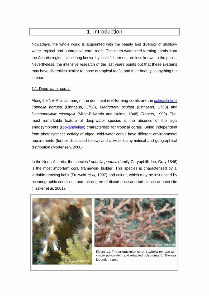
Figure 1.1 The scleractinian coral Lophelia pertusa with visible polyps (left) and retracted polyps (right), Theresa Mound, Ireland. Copyright IFREMER

Copyright IFREMER

1.2. Distribution of Lophelia pertusa

The species Lophelia pertusa was firstly recognised in the early nineteenth century

after the recovery of specimens by Scottish fishermen (Wilson, 1979). Up till now,

this coral has been found throughout the North Atlantic but also more southward,

along the coasts of Africa and Brazil. Records show that the species occurs in parts

of the Mediterranean, in the Pacific and the Indian Ocean (Mortensen, 2000 and

Rogers, 1999). Globally, Lophelia can be found at depths from 39 to 3380 m

(Mortensen, 2000) with an optimum between 250 and 450 m (Frederiksen et al,

1992). Water temperature ranges from 4 to 12 degrees (Rogers, 1999) and salinity

from 31.85 to 37 PSU (Practical Salinity Unit) (Strömgren, 1971; Le Danois, 1948

and Freiwald, 1998).

Several hypotheses have been proposed about the habitat preferences of the

species (Rogers, 1999 and Mortensen, 2000):

1.2.1 Substrate

Lophelia needs hard substrates to settle on; this can be morainic boulders, pebbles

or even shell debris and polychaete tubes. The dead coral branches of the first

colony form new settling substrates.

1.2.2 Water-masses, currents and their influence on food-availability

The depth at which Lophelia is found varies largely. On the Norwegian/Scottish shelf

and around the Faroe Islands, the coral occurs most frequently between 200m and

400m depth (Teichert, 1958 & Frederiksen et al, 1992). Around western Ireland and

in the Bay of Biskay, the coral occurs between 200 and 1000m depth (Le Danois,

1948 and Kenyon et al, 1998). Frederiksen et al (1992) studied the occurrence of

Lophelia pertusa off the Faroe Islands. They suggested that the depth distribution of

Figure 1.2 Global distribution of the scleractinian coral Lophelia pertusaaccording to Rogers (1999).

Lophelia could depend on the maximal wave action, as this coral is very fragile and

can tip over at low current speeds. They also stress the importance of temperature

as a limiting factor, as North-Atlantic Lophelia occurs in the presence of cool Atlantic

water. Freiwald (1998) found a relation between the occurrence of the thermocline

and the growth rate of Lophelia in Norwegian water (Stjernsund Sill). Above the

thermocline, the fjord waters show seasonal fluctuations with respect to temperature

and salinity, while below the inflowing Atlantic water it remains stable throughout the

year.

According to Frederiksen et al (1992), the occurrence of Lophelia around the Faroe

Islands is correlated with bottom slopes critical to internal tidal waves. The breaking

of the waves can increase food supply to the corals by resuspension of organic

matter from the bottom and by increasing the vertical nutrient flux through the

thermocline. This flux can in turn increase the phytoplankton production and the

vertical flux of flocculent organic particulate matter.

Mortensen et al (in press) showed that the density of reefs on the Norwegian shelf is

positively correlated with the seafloor topography, with reefs occurring on local

elevations. This could be due to the local increase in encounter rate of food particles

caused by a higher current velocity (Frederiksen et al, 1992). The currents also

remove waste and keep corals and substratum free of sediments, which can impair

feeding and larval settlement.

1.2.3 Seepage of hydrocarbons

Hovland and colleagues proposed a theory stating that Lophelia reefs are formed at

locations characterized by high concentrations of seeping fluids and gasses. These

substances provide the energy and carbon source for deep-water ecosystems that

grow independent from photosynthesis. Hydrocarbons can feed a variety of

microorganisms, on which the Lophelia ecosystem can grow. Indicators for

hydrocarbon seepage are pockmarks and high values of light hydrocarbons like

methane and ethane in the sediment. Gas-charged layers can be detected on

seismic records (e.g. Hovland & Thomsen, 1997; see also Geological handbook).

This theory would explain the conical growth pattern (corals grow symmetrically

around the energy source, instead of linear as expected in the case of current

dependency) of mounds like they can be found in the Norwegian Sula reef and

Haltenpipe reefs (Hovland et al, 1998). However, Lophelia does not grow on every

location with hydrocarbon seepage, so other controlling factors have to be taken into

account.

In addition to the theory of Hovland & Thomsen (1997), Henriet et al (1998)

suggested that the decay of a gas hydrate horizon in the “Magellan” mound province,

Porcupine Seabight, might have fuelled methane seeps, which in turn could support

coral growth.

1.3. Lophelia and human activities

Ecosystems formed by Lophelia have been studied intensively during the last ten

years during programs like ACES (Atlantic Coral Ecosystem Study), Geomound and

Ecomound. This is mainly due to the increasing exploitation of hydrocarbons (oil and

gas) and fish (e.g. fish in figure

1.4) on the continental margins

(Mortensen, 2000). These

activities pose a serious threat to

the survival of Lophelia

ecosystems.

Deep-sea fish trawling nets

break up the coral colonies and

broken lines and entangled nets

keep killing fish, crabs and other

animals that get stuck in them

(ghost fishing). Next to the direct

impacts, the trawling also causes

indirect damage by changing the hydrodynamic and sedimentary conditions. Trawls

resuspend sediment that can clog up the respiratory and feeding structures of

Lophelia and associated fauna downstream. Trawling may also level off the seabed

by scraping off high points, filling in depressions and moving boulders. Since

Lophelia seems to need high points to grow on (see 1.2), trawling can make the

seabed unsuitable for growth (Tasker et al, 2001). Another result of fishing can be an

alteration of the amount of reef- eroding species, which can influence the balance

between reef building and reef-erosion (Rogers, 1999).

The consequences of trawling and other activities can be studied using an ROV or

other remote sensing techniques like side scan sonar, which can reveal trawl marks

on the seafloor. The net on figure 1.3 was found during a dive on Theresa Mound

with ROV Victor 6000 from the IFREMER institute.

As for the hydrocarbon exploitation, the main menaces are:

q Release of mud, sand and water contaminated with chemicals and oil

Figure 1.3 Abandoned net on Theresa Mound, Ireland.

Copyright IFREMER

q Mechanical damage to the seafloor due to construction works and

anchoring

Drilling mud does not only increase the sedimentation rate, which disturbs the

feeding of Lophelia; it also influences calcification, physiology and polyp expansion

and retraction (Rogers, 1999).

Copyright IFREMER

Figure 1.4 Phycis blennoides (forkbeard) at the left is an exploited deep-sea species, found living among Lophelia (Theresa mound, Ireland). The picture on the right is the commercial fish Pollachius virens or saithe (Haltenpipe, Norway).

STATOIL

2. Material and methods

2.1 Locating and mapping

The knowledge of local fisherman has proved to be very useful for locating cold-

water reefs unknown to the scientific world (Wilson, 1979 and Mortensen, 2000). The

subsequent precise positioning and mapping by scientists is done using side scan

sonar images, high resolution sub bottom profilers, seismic profiles and multi-beam

bathymetry (e.g. De Mol et al, in press; Mortensen, 2000; Hovland et al, 1998;

Hovland et al, in press). Coral-banks can be recognized by their anomalously steep

surface gradients and isolated occurrence (Hovland et al, 1998). Chapter II of the

geological handbook (gas and fluids in marine sediments and related phenomena)

gives a detailed overview of the functioning and outputs of side scan sonar, high-

resolution sub bottom profilers and seismic systems.

Copyright IFREMER

Figure 2.2 High resolution sub bottom profile from Hovland Mounds, northern slope of Porcupine Basin, Ireland (Veerle Huvenne). Sub bottom imagesgive information about the upper layers of the seafloor.

Figure 2.1 3D model of Theresa mound, Ireland, based on multi-beam bathymetry. Bathymetry is basically the measurement of depths by recording the travel time from the acoustic source to the seafloor and back. The colours represent differences in height.

Copyright IFREMER

Figure 2.3. Adapted side scan sonar image from the Hovland Mounds, Ireland. The white side of the mounds are directed towards the towfish, the black side is the acoustic shadow (positive sonograph). Side scan sonar images give information about topography and seafloor characteristics. (image Veerle Huvenne)

Cross-section

2.2 Sampling

Sampling is necessary for the interpretation of the acquired data and for detailed

geological and biological investigations. Different gears and methods have been

used during the study of the distribution and morphology of Lophelia and the

composition of the associated fauna. The choice of sampling device depends on a

large number of factors like the available vessel, the location of and access to the

sampling site, the number of samples to be taken, the weather and of course the

available budget. In this chapter, only the devices that are frequently used for

biological sampling will be discussed.

2.2.1 Dredge

A dredge sampler consists of a cutting edge furnished with hardened steel teeth.

During dragging, the edge penetrates into the sediment. Biological or mineralogical

material is collected in a nylon or canvas bag of variable mesh size. Dredging mostly

yields large qualitative samples but these are not representative for a single point

and the finer fraction of the sample may be washed out during recovery (Larson et al,

Figure 2.4 2D high resolution sparker profile (seismic profile) of Theresa Mound (BEL35) and her neighbour (BEL36), Ireland. The upper part of the figure shows the original seismic profile, the lower part shows the interpretation. The vertical scale indicates time in seconds. This Two Way Travel Time (TWT or TTWT) represents the time needed by the sound wave to travel from the sparker to a horizon in thebottom and back (image Ben De Mol).

Theresa

1997). Although dredge samples are/were frequently used in the research regarding

Lophelia reefs (Stetson et al, 1962; Wilson, 1979; Mortensen, 2000; Jensen &

Frederiksen, 1992, De Mol et al, in press, Freiwald et al, 1997), alternative sampling

devices are preferable because of the destructive effects of dredging and the

inadequate sampling of mobile fauna (Gage & Tyler, 1996 and Mortensen, 2000).

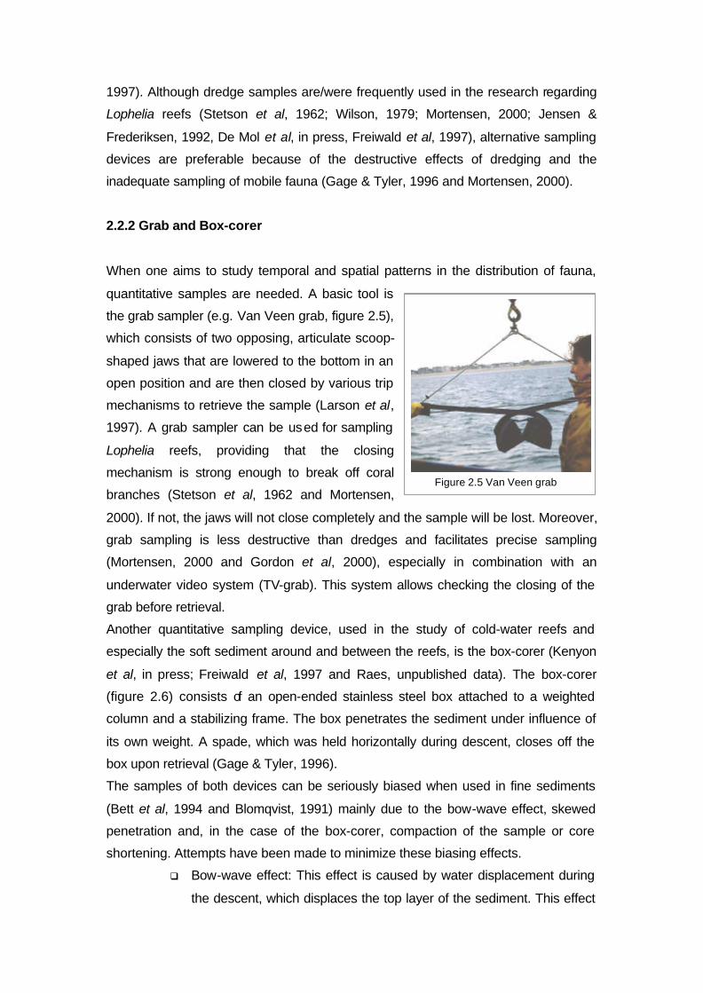
2.2.2 Grab and Box-corer

When one aims to study temporal and spatial patterns in the distribution of fauna,

quantitative samples are needed. A basic tool is

the grab sampler (e.g. Van Veen grab, figure 2.5),

which consists of two opposing, articulate scoop-

shaped jaws that are lowered to the bottom in an

open position and are then closed by various trip

mechanisms to retrieve the sample (Larson et al,

1997). A grab sampler can be used for sampling

Lophelia reefs, providing that the closing

mechanism is strong enough to break off coral

branches (Stetson et al, 1962 and Mortensen,

2000). If not, the jaws will not close completely and the sample will be lost. Moreover,

grab sampling is less destructive than dredges and facilitates precise sampling

(Mortensen, 2000 and Gordon et al, 2000), especially in combination with an

underwater video system (TV-grab). This system allows checking the closing of the

grab before retrieval.

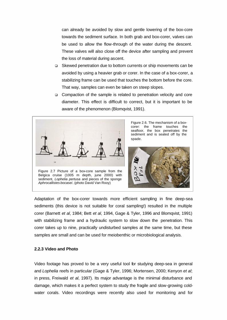
Another quantitative sampling device, used in the study of cold-water reefs and

especially the soft sediment around and between the reefs, is the box-corer (Kenyon

et al, in press; Freiwald et al, 1997 and Raes, unpublished data). The box-corer

(figure 2.6) consists of an open-ended stainless steel box attached to a weighted

column and a stabilizing frame. The box penetrates the sediment under influence of

its own weight. A spade, which was held horizontally during descent, closes off the

box upon retrieval (Gage & Tyler, 1996).

The samples of both devices can be seriously biased when used in fine sediments

(Bett et al, 1994 and Blomqvist, 1991) mainly due to the bow-wave effect, skewed

penetration and, in the case of the box-corer, compaction of the sample or core

shortening. Attempts have been made to minimize these biasing effects.

q Bow-wave effect: This effect is caused by water displacement during

the descent, which displaces the top layer of the sediment. This effect

Figure 2.5 Van Veen grab

can already be avoided by slow and gentle lowering of the box-core

towards the sediment surface. In both grab and box-corer, valves can

be used to allow the flow-through of the water during the descent.

These valves will also close off the device after sampling and prevent

the loss of material during ascent.

q Skewed penetration due to bottom currents or ship movements can be

avoided by using a heavier grab or corer. In the case of a box-corer, a

stabilizing frame can be used that touches the bottom before the core.

That way, samples can even be taken on steep slopes.

q Compaction of the sample is related to penetration velocity and core

diameter. This effect is difficult to correct, but it is important to be

aware of the phenomenon (Blomqvist, 1991).

Adaptation of the box-corer towards more efficient sampling in fine deep-sea

sediments (this device is not suitable for coral sampling!) resulted in the multiple

corer (Barnett et al, 1984; Bett et al, 1994, Gage & Tyler, 1996 and Blomqvist, 1991)

with stabilizing frame and a hydraulic system to slow down the penetration. This

corer takes up to nine, practically undisturbed samples at the same time, but these

samples are small and can be used for meiobenthic or microbiological analysis.

2.2.3 Video and Photo

Video footage has proved to be a very useful tool for studying deep-sea in general

and Lophelia reefs in particular (Gage & Tyler, 1996; Mortensen, 2000; Kenyon et al;

in press, Freiwald et al, 1997). Its major advantage is the minimal disturbance and

damage, which makes it a perfect system to study the fragile and slow-growing cold-

water corals. Video recordings were recently also used for monitoring and for

Figure 2.6. The mechanism of a box-corer: the frame touches the seafloor, the box penetrates the sediment and is sealed off by the spade.

Figure 2.7 Picture of a box-core sample from the Belgica cruise (1005 m depth, june 2000) with sediment, Lophelia pertusa and pieces of the sponge Aphrocallistes bocasei . (photo David Van Rooy)

defining the successional stages in deep-sea ecosystems (Gutt & Starmans, 2001).

Vetter and Dayton (1998 & 1999) used video images for studying submarine

canyons. The quality of the images has significantly improved over the last decades,

among other things by using ROV ‘s (Remotely Operated Vehicles), with which

kilometre-long transects with a large amount of high resolution information can be

obtained in a short period of time. The information about bottom sediment type and

epibenthic fauna complements other sampling

techniques like dredges, grabs or corers

(Vorberg & van Bernem, 1998).

In situ samples can be taken with the ROV ’s

robotic arms (figure 2.8). However, ROV ‘s are

very expensive and heavy, so they require a

ship with adapted winches and cables. A

cheaper alternative is the already mentioned

TV-grab, which is easier to operate

(Mortensen, 2000).

Analysis of underwater video images,

however, brings about some difficulties and imperfections.

q Only the recognisable epibenthic megafauna (> 5cm or more, depending on

the height of the camera above the seabed and the quality of the film) can be

identified. A part of these organisms will not be visible on the image because

they can be hidden between branches, under rocks, etc. Accordingly, one has

to anticipate an underestimation of both diversity and density.

q When identifying living organisms, one has to take into account the different

appearances of an organism (e.g. coral with or without its polyps sticking out).

Moreover, only one side of the animal is visible on film. It can therefore be

difficult to identify an organism when the determinative features are situated

on the ventral side of the organism. A similar problem appears while trying to

identify sponges: spicules (=skeletal elements) are needed for identification.

Morphology alone does not suffice.

q The density of individuals of a species can be so high on a certain location

Figure 2.8 In situ sampling with arm of ROV Victor during the Caracole cruise (2001), Theresa Mound, Ireland.

Copyright IFREMER

Figure 2.9. Field of crinoids from Haltenpipe, Norway

STATOIL

that discerning the separate organisms and counting them can become a

difficult task (e.g. crinoids in figure 2.9).

q The size of the recorded area will not be the same along the whole transect,

due to vertical movements of the camera or the ROV, and changes in towing

speed. Therefore, standardizing the number of organisms will be impossible,

unless some measure of the size of the area is included on the image. A lead

weight (e.g. TTR-TVAT) or laser beams (Gutt & Starmans, 2001 and

Starmans et al, 1999) can indicate the width of the video line.

q In order to define zonation patterns using video footage, the trajectory of the

ROV or the camera has to be established using GPS (Global Positioning

System).

In addition to, or apart from video images, still photographs can be taken (Stetson,

1962; Gutt & Starmans, 2001 and Starmans et al, 1999). These photos can facilitate

the identification of the megafauna and usually have a higher resolution than

underwater video (Gordon et al, 2000). Systems like ‘Bathysnap’ (Gage & Tyler,

1996), which are put on the seafloor for a long period of time and take pictures at

regular intervals, allow the determination of temporal changes in deep-sea

environments.

3. Species associated with living and dead Lophelia

3.1 Introduction

The main aim of this chapter is to briefly introduce the large megafaunal taxa and

their characteristics to non-biologists and to bring you into contact with some

representative species that were observed on Lophelia reefs. In that way, you will be

able to extract more information from images and species lists, and you will better

understand the ecological exercises.

As there are large differences in faunal composition between different sites,

examples will be given from both Norwegian reefs (in particular the Haltenpipe reef)

and Irish reefs (in particular Theresa Mound).

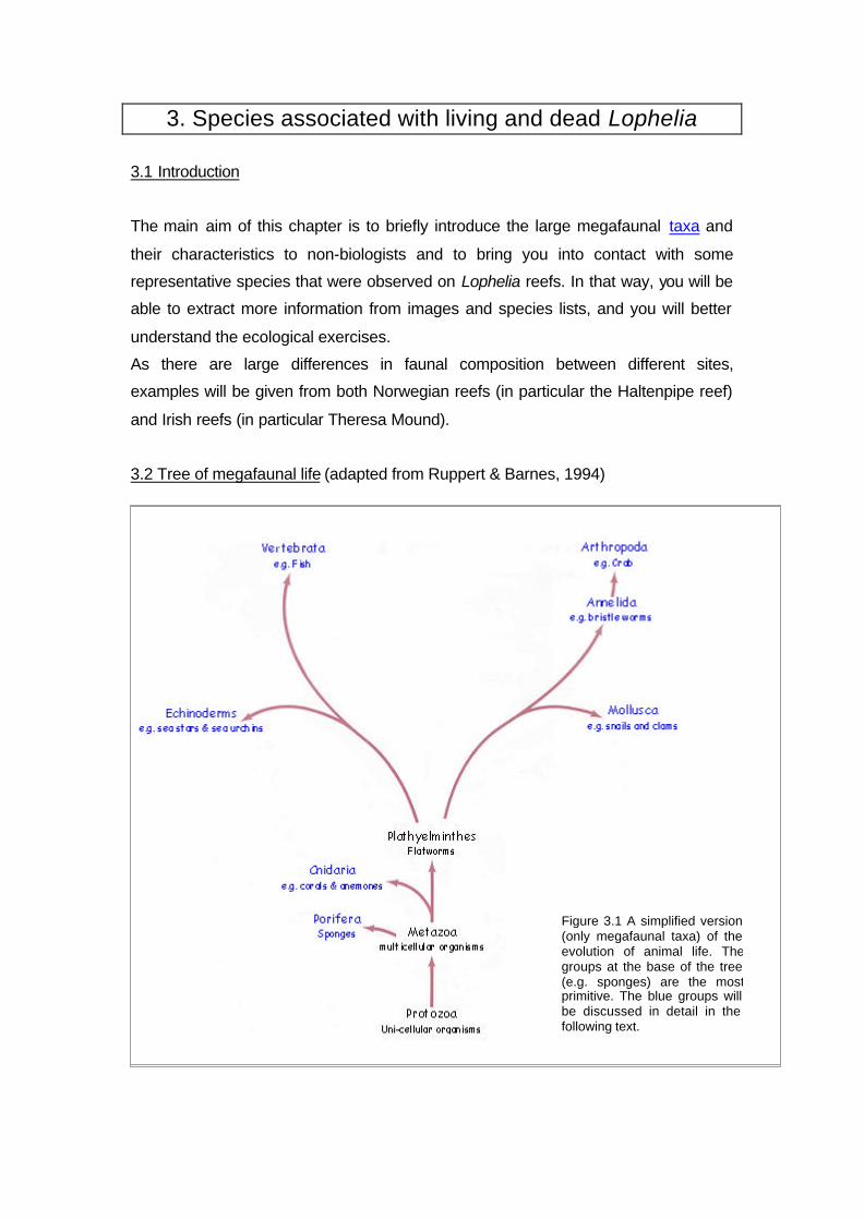
3.2 Tree of megafaunal life (adapted from Ruppert & Barnes, 1994)

Figure 3.1 A simplified version (only megafaunal taxa) of the evolution of animal life. The groups at the base of the tree (e.g. sponges) are the most primitive. The blue groups will be discussed in detail in the following text.

3.3 Megafaunal groups, their characteristics and examples

3.3.1 Porifera (sponges)

Sponges are the most primitive of

multicellular organisms. They lack

organs but they have a well-

developed connective tissue that

builds up the sessile body around a

system of water canals. The water

flow through the body, created by the

beating of flagella, provides oxygen

and food and removes waste, sperm

and larvae.

Feeding type: mainly filter feeders

Taxonomy: subdivision mainly based

on shape and composition of the

skeletal elements => calcareous,

siliceous (glass sponges), spongin

fibers or combinations of the former

3.3.2 Cnidaria (hydras, jellyfish, sea anemones and corals)

Cnidarians are aquatic, radially symmetrical animals with tentacles encircling the

mouth. Food is caught using tentacles and is immobilized by specialized cells

(cnidocytes). Unlike the sponges, these animals do have a gut. Cnidarians can

exhibit two body forms: the pelagic medusa (jellyfish) and the benthic, sessile polyp.

Feeding type: carnivores – suspension feeders

Taxonomy: subdivision based on importance of one of the two body forms (medusa

or polyp) and on morphological features (e.g. type of gametes and cnidocytes,

number of tentacles, presence and characteristics of a skeleton).

The species Lophelia pertusa, the key species in Atlantic deep-water reefs, is a

scleractinian coral with a branching calcium carbonate skeleton. Lophelia is a

pseudocolonial species, meaning that it produces a skeleton by cloning but the

polyps are not interconnected with a neural network (Mortensen, 2000). Little is

known about reproduction, larval biology and recruitment (Rogers, 1999).

Figure 3.2. The upper species is the glass sponge Aphrocallistes bocasei, which is a dominant element in the biological assemblage of Theresa Mound, Ireland. The left picture shows Mycale lingua, which can overgrow Lophelia colonies (Haltenpipe, Norway).

Copyright IFREMER

STATOIL

3.3.3 Annelida: Polychaeta (bristle worms)

The body form of polychaetes varies widely, reflecting a range of life styles from

swimming, through crawling, to active burrowing or tube dwelling. The generalized

polychaete body plan is segmented, with each segment bearing a pair of lateral

appendages (parapods). The anterior end of the worm is the prostomium, which

bears sense organs. The mouth is situated ventrally, following the prostomium. The

terminal unsegmented region, the pygidium, carries the anus.

A large number of species have already been found in samples from Lophelia reefs

(e.g. Eunice norvegica, which shows an interspecific relationship with Lophelia

pertusa (Mortensen, 2000)). In video-footage and still photographs, only the biggest

species can be discerned and those are mainly belonging to the group of Sabellidae

or fan worms, which are filter feeders and tube builders.

Feeding type: carnivores, filter feeders, herbivores, omnivores, scavengers, browsers

and deposit feeders.

Taxonomy: subdivisions are based on morphological adaptations to the type of

feeding and locomotion (e.g. shape of parapods, presence of gills, shape of

prostomial appendages, presence of jaws) The sabellid worm Sabella pavonina can be seen on video segment 4 on the CD in the back of the

handbook.

3.3.4 Mollusca (clams, oysters, squids, octopods and snails)

Moluscs generally have a muscular foot, a calcareous shell that is secreted by the

underlying body wall (the mantle), and a feeding organ (the radula). They can

possess several pairs of gills in their mantle cavity.

Figure 3.3. A. The stony coral Lophelia pertusa, note the redfish

Sebastes viviparus (Haltenpipe, Norway) B. The octocoral (8 tentacles) Paragorgia arborea, with

red and white variety (left) from Haltenpipe, Norway C. A little anemone on octocoral Paramuricea placomus ?

(Theresa Mound, Ireland) D. Two anemones (Bolocera thuediae?) – in the middle

the crab Lithodes maja (Haltenpipe, Norway)

A B C

D

STATOIL STATOIL

STATOIL

Copyright IFREMER

On the investigated video footage and photographs from the Haltenpipe A reef in

Norway and Theresa Mound in Ireland, only representatives of the subgroups

Gastropoda (snails) and Bivalvia (clams) were encountered.

Gastropoda usually have a coiled shell and they use their foot for locomotion.

Feeding type: highly variable (herbivores,

carnivores, scavengers, deposit feeders,

suspension feeders and parasites).

Taxonomy: subdivisions are based on the

shape of the shell and on internal features like

the number and position of gills, the shape of

the teeth on the radula etc.

Bivalvia are characterized by a

reduced head and a laterally compressed

body covered by a bivalved shell. They do not

possess a radula because they are mostly

filterfeeders. Their foot is compressed and

adapted for burrowing.

Feeding type: deposit feeders or filter feeders

Taxonomy: the different groups can be

recognized by the shape of their shells

3.3.5 Arthropoda: Crustacea (crabs, shrimps, lobsters, etc.)

Crustaceans are mainly marine

organisms with 5 pairs of head

appendages, a segmented trunk, which

can be covered with a shield (= the

carapace) and trunk appendages; all

with varying degrees of specialization.

Within the megafauna, only benthic

Decapods (with five pairs of legs) were

observed on film and photographs

(figures 3.3 and 3.5). Their first pair of

legs, like in the genus Munida, can be

enlarged and used for grabbing prey.

Decapod gills are very well enclosed in the carapace.

Feeding type: predators and scavengers

Figure 3.4. The upper picture shows an unidentified gastropod on Lophelia, characterized by its coiled shell (Theresa Mound, Ireland). The lower picture shows a cluster of bivalves of the species Acesta excavata (Haltenpipe, Norway). See also video fragment 1 on the CD: Acesta excavata.

Copyright IFREMER

STATOIL

Figure 3.5. Decapods from Theresa Mound, Ireland. The picture shows one crab (bottom) and two squat lobsters from the genus Munida. This animal is also very common in Norwegian reefs.

Copyright IFREMER

Taxonomy of Decapoda: identification based on shape of legs and carapace,

development of the abdomen, shape of antennae, etc.

3.3.6 Echinodermata (sea stars, sea urchins, sea cucumbers, brittle stars and

sea lilies / feather stars)

Echinoderms are marine bottom dwelling organisms with a pentamerous radial

symmetry. All groups have a skeleton that consists of articulating or fused calcareous

plates that bear spines or tubercles.

Asteroidea or sea stars mostly have five arms, which are grading into a

central disc. They can move using their large number of

tube feet at the ventral side of the arms. This group is

also known for its high regenerative power: arms can

grow back and even a new star can grow from one arm

with a piece of disc.

Feeding type: most species are carnivores and

scavengers

Taxonomy: based on features like the shape of the tube

feet, skeletal plates, disc and spines

Ophiuroidea or brittle stars differ from sea stars with their long arms that are

more sharply set off from the disc. The arms are more solid and the tube feet only

play a little role in locomotion. The mouth is situated on the ventral side of the disc

and is surrounded by large plates and five jaws for chewing.

Feeding type: scavenging, deposit feeding and filter feeding

Taxonomy: based on presence and shape of papillae on jaws and structure of

skeletal plates

Echinoidea or sea urchins are circular or oval and have no arms. Their

skeleton is fused into a solid armour and covered with movable spines. These

spines, together with tube feet, are used for locomotion.

Figure 3.7. The sea urchin on the right is a specimen of the species Cidaris cidaris, which is commonly found on Lophelia reefs (Haltenpipe, Norway). The picture on the left shows Echinus sp., observed on Theresa Mound, Ireland.

Copyright IFREMER STATOIL

Figure 3.6. On the left a sea star (Asteroidea) and on the right a brittle star (Ophiuroidea), both from Haltenpipe, Norway.

STATOIL STATOIL

Feeding type: sea urchins feed by scraping off detritus or encrusting organisms and

algae, using a complex scraping apparatus: grazing

Taxonomy: identification based on development of scraping system, position of tube

feet, number of spines, etc.

Crinoidea are primitive echinoderms that can be stalked

(sea lilies) or free-living (feather stars). The latter can attach

themselves to the substrate with grasping organs (cirri). Unlike

sea stars, sea urchins and brittle stars, crinoids have an upwards-

directed mouth. Crinoids feed by filtering particles out of the water

column, using a crown of featherlike arms surrounding the mouth.

Feeding type: suspension feeders

Taxonomy: subdivisions are based on the presence/absence of a

stalk, the length of the arms and the shape of the cirri and the

basal structure (centro-dorsal) to which the cirri are attached.

Holothuroidea or sea cucumbers were not observed on

the studied films and pictures, although they are very abundant

on soft deep-sea bottom.

3.3.7 Vertebrata: Pisces (fish)

Fish are aquatic vertebrates that breathe by means of gills. This group comprises

jawless fish (Agnatha), cartilaginous fish (Chondrichthyes, e.g. sharks and rays) and

bony fish

(Osteichthyes,

e.g. cod and

salmon).

Feeding type:

various, but all

the species

observed on

the studied

film and

photographs

are carnivorous.

Taxa: subdivisions are based on the shape of the whole body, of the fins, the scales,

the lateral line system etc. The redfish Sebastes viviparus can be seen on video fragment 2 on the CD, together with the

anemone Bolocera thuediae

Figure 3.8. Crinoids (Hathrometra sarsi) on the underside of a buoy on the Ha ltenpipe reef, Norway.

STATOIL

Figure 3.9. Bony fish A. Lepidion eques (Theresa

Mound, Ireland) B. Angler fish Lophius sp.

(Theresa Mound, Ireland) C. Tusk (Brosme brosme)

from Haltenpipe, Norway

A B

Copyright IFREMER

Copyright IFREMER

C

STATOIL

4. Diversity 4.1 General

Biodiversity is a term used to describe the rich variation of life on earth. Diversity can

concern gene pools, species communities or landscapes, which are respectively

composed of genes, species communities and habitats (Heip et al, 1998).

Hill (1973) defined the diversity of a community as ‘a parameter describing the

complexity of the environment, the interspecific relations and the stability of the

community’.

When describing the diversity of a biological community, one has to consider two

components:

• Species richness representing the number of species encountered in the

investigated community

• Evenness representing the spreading of the individuals in the community

over the different species

Over the years, a high variety of indices and visual plots have been developed for

use in different circumstances and with more emphasis on either species richness or

evenness. When choosing an index or plot to describe a certain community, several

questions have to be asked:

• What is the weight you want to give to dominant and/or rare species in

the community?

• Do you want to compare with other studies and what statistics do you

want to apply?

• Are the samples of the same size and what was the sampling

strategy?

Different diversity-indices summarise slightly different aspects of species

assemblages. Therefore it is useful to calculate and compare different indices

obtained using species abundances from the assemblages (Heip et al, 1998).

4.1.1. How to calculate species diversity? The basis of a community analysis is primarily a matrix containing stations/samples

as columns and species as rows. The entries of the matrix are mostly abundances.

Together with the appropriate formulae, these data in a worksheet (e.g. Microsoft

Excel) can be used for calculating diversities or for making a plot that allows

comparing diversities of different samples or stations. In the following paragraphs,

the most frequently used diversity indices and plots will be briefly discussed. They

will be further elaborated in the exercises.

4.1.2. Shannon-Wiener diversity index:

The Shannon-Wiener index is a measure of the uncertainty in predicting to what

species an individual drawn from a collection of S species and N individuals will

belong (Ludwig & Reynolds, 1988). The higher the index, the higher the biodiversity.

ð Can be used to compare habitats based on different sample sizes

ð Sensitive about rare species

ð Commonly used index in the study of Lophelia’s associated fauna (e.g.

Jensen & Frederiksen, 1992 and Mortensen, 2000)

The evenness can be expressed as: J = H’/ ln S where S represents the number of

species in the sample. Evenness assumes a value between 0 and 1.

4.1.3. K-dominance curve

This method graphically displays the distribution (rare or common) of species in

different samples. The K-dominance or cumulative abundance (i.e. the percentage

made up by the k-th-most dominant species plus all more dominant species) is

with Ni: number of individuals of the species I in

the sample, and N: total number of individuals,

(Ni/N) = pi

)/ln()/(' NNNNH ii∑−=

species abundances

samples

Figure 4.1. Excel spreadsheet with species (first column), samples (first row) and species abundances per sample (entries of matrix).

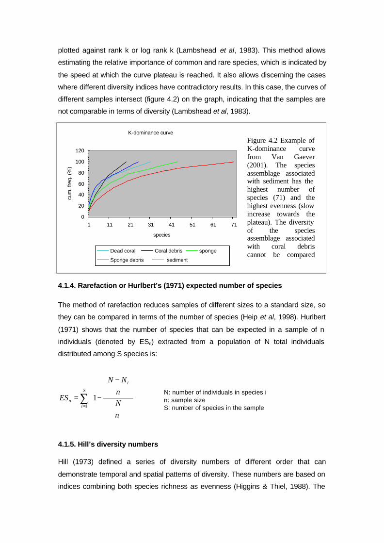
plotted against rank k or log rank k (Lambshead et al, 1983). This method allows

estimating the relative importance of common and rare species, which is indicated by

the speed at which the curve plateau is reached. It also allows discerning the cases

where different diversity indices have contradictory results. In this case, the curves of

different samples intersect (figure 4.2) on the graph, indicating that the samples are

not comparable in terms of diversity (Lambshead et al, 1983).

4.1.4. Rarefaction or Hurlbert’s (1971) expected number of species The method of rarefaction reduces samples of different sizes to a standard size, so

they can be compared in terms of the number of species (Heip et al, 1998). Hurlbert

(1971) shows that the number of species that can be expected in a sample of n

individuals (denoted by ESn) extracted from a population of N total individuals

distributed among S species is:

4.1.5. Hill’s diversity numbers Hill (1973) defined a series of diversity numbers of different order that can

demonstrate temporal and spatial patterns of diversity. These numbers are based on

indices combining both species richness as evenness (Higgins & Thiel, 1988). The

N: number of individuals in species i n: sample size S: number of species in the sample

∑=

−

−=S

i

i

n

n

Nn

NN

ES1

1

K-dominance curve

0

20

40 60

80

100

120

1 11 21 31 41 51 61 71 species

cum

. fre

q. (%

)

Dead coral Coral debris sponge Sponge debris sediment

Figure 4.2 Example of K-dominance curve from Van Gaever (2001). The species assemblage associated with sediment has the highest number of species (71) and the highest evenness (slow increase towards the plateau). The diversity of the species assemblage associated with coral debris cannot be compared with the species

diversity number of order a is defined as: ( ) ( )aan

aa pppN1/1

21 ... +++= with pn the

proportional abundance of species n in the sample. Different diversity numbers can

be used:

ð N0 represents the number of species in the sample. No distinction is made

between rare and dominant species.

ð N1 = exp (H) where H is the Shannon-Wiener index, which attaches less

importance to the rare taxa than N0:

ð N2 = the reciprocal of Simpson’s diversity index:

∑=

=S

iip

D

1

2

1

Simpson’s index, which varies from 0 to 1, gives the probability that two

individuals drawn at random from a population belong to the same species

(Ludwig & Reynolds, 1988).

ð Ninf = the reciprocal of the proportional abundance of the most dominant taxa

and is also named the ‘dominance-index’. This number only takes into

account the most dominant species: Ninf = 1−ip

Soetaert and Heip (1990) tested the sample size dependency of different diversity

indices, including Hill’s diversity numbers. They concluded that high-diversity

communities and the use of indices, which are sensitive to rare species, require

larger samples.

4.2 Biodiversity associated with Lophelia reefs

Several studies on the associated fauna of cold-water corals have already been

carried out, with samples and images from different areas (Mortensen et al, 1995;

)ln()(' ii ppH ∑−=

Number of individuals

Num

ber o

f spe

cies

N0

N1

N2

Ninf

Figure 4.3 Hill’s diversity numbers and sample size dependency (adapted from Soetaert & Heip, 1990). This graph indicates that the indices N0 and N1 are the most dependent on sample size: with increasing sampling effort, more and more rare species will be found. Ninf is independent from sample size: only the most common species, which will also be present in small samples, is considered. Sample size dependency increases with diversity: more rare species, thus larger samples have to be taken in order to estimate diversity.

ES

Jensen & Frederiksen, 1992). A few results and trends seem to be common and will

be briefly discussed in this chapter.

4.2.1 Deep-sea coral reefs versus tropical reefs Generally, Lophelia reefs are considered to be very diverse. In fact, the diversity is

almost equal to that of tropical, hermatypic (containing zooxanthellae) scleractinians

(Jensen and Frederiksen, 1991). This high diversity is mainly caused by the following

factors:

q The complex 3D structure of the corals, which creates a high variety of

suitable habitats for the associated fauna. Mortensen (1995) discerns

four different microhabitats: (1) the smooth surface of living Lophelia,

(2) the detritus laden surface of dead Lophelia, (3) the cavities inside

dead Lophelia made by boring organisms and (4) the space between

the coral branches.

q The age and size of the colonies, and the stability of the deep-sea

environment allowed the development of complex interspecies

interactions and specialisations.

However, the diversity of tropical coral reefs is still higher than that of Lophelia reefs.

This can be explained by the high variety of Scleractinia, each with their associated

fauna. Additionally, deep-sea coral reefs lack macro-algae, which contribute largely

to the structural habitat complexity of tropical reefs and are important food sources

for associated organisms. Finally, tropical reefs are older than deep-water reefs so

there was more time for establishing a high diversity of associated organisms

(Mortensen, 2000).

4.2.2 Biodiversity within Lophelia reefs Mortensen et al (1995) demonstrated that the diversity of megafauna is higher in

areas of dead Lophelia compared to that of living coral. The same pattern appeared

in the case of macrofaunal (smaller, more individuals and more species) diversity

(Jensen & Frederiksen, 1992). The low number of species found on living Lophelia

may be due to antifouling properties of the living tissue; or the living substrate may be

to unstable for settlement. Next to the differences in diversity between living and

dead coral, there is also a remarkable difference between the reefs and the

surrounding sediment. Mortensen (2000) found that the Shannon-Wiener index was

three times higher on the reefs.

5. Communities

5.1 Definition

A community can be defined as “ an assemblage of species populations that occur

together in space and time.” (Begon et al, 1996) or “ the total set of organisms in an

ecological unit (biotope)” (Heip et al, 1998). However, a community is more than only

an assemblage of species in a certain area. An important part of the community

structure is made up by interactions between the species and their populations, like

predation and competition. Examples of how these interactions can influence the

community structure are frequently encountered in tropical coral reefs:

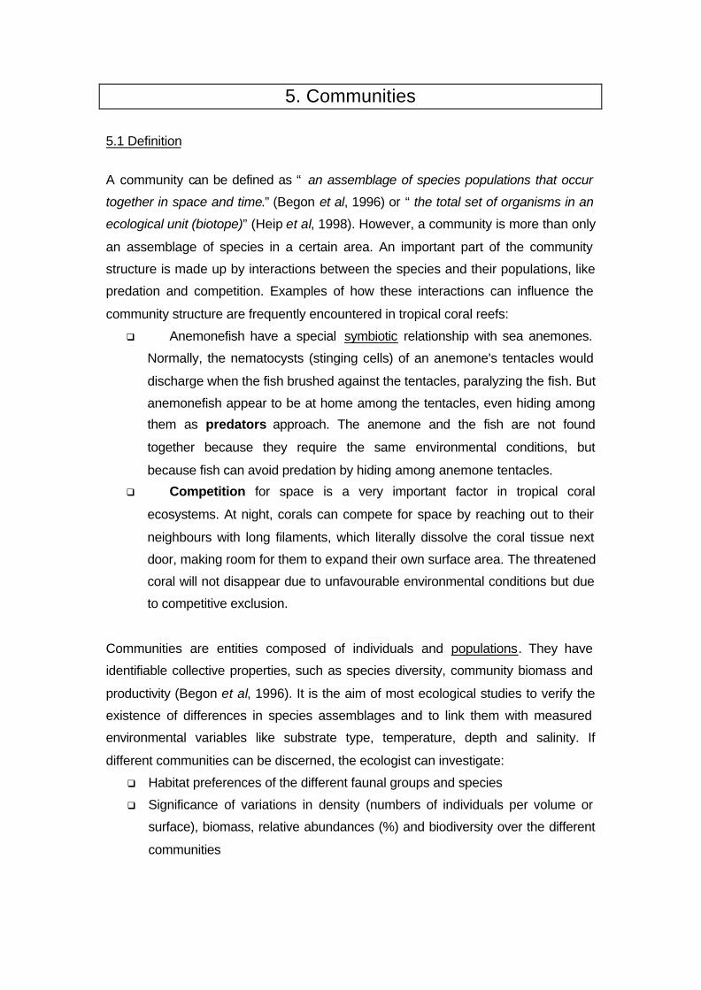
q Anemonefish have a special symbiotic relationship with sea anemones.

Normally, the nematocysts (stinging cells) of an anemone's tentacles would

discharge when the fish brushed against the tentacles, paralyzing the fish. But

anemonefish appear to be at home among the tentacles, even hiding among

them as predators approach. The anemone and the fish are not found

together because they require the same environmental conditions, but

because fish can avoid predation by hiding among anemone tentacles.

q Competition for space is a very important factor in tropical coral

ecosystems. At night, corals can compete for space by reaching out to their

neighbours with long filaments, which literally dissolve the coral tissue next

door, making room for them to expand their own surface area. The threatened

coral will not disappear due to unfavourable environmental conditions but due

to competitive exclusion.

Communities are entities composed of individuals and populations. They have

identifiable collective properties, such as species diversity, community biomass and

productivity (Begon et al, 1996). It is the aim of most ecological studies to verify the

existence of differences in species assemblages and to link them with measured

environmental variables like substrate type, temperature, depth and salinity. If

different communities can be discerned, the ecologist can investigate:

q Habitat preferences of the different faunal groups and species

q Significance of variations in density (numbers of individuals per volume or

surface), biomass, relative abundances (%) and biodiversity over the different

communities

5.2 How are communities defined?

The analysis of communities begins with collecting data on the species assemblages

and the environmental variables of the investigated area. This results in complex

data matrices with information about the encountered species (number of individuals

per volume or surface, see figure 4.1) and different environmental variables (depth,

salinity, current velocity, seafloor characteristics, etc.) per sample like in figure 5.1

where substrate for epifaunal communities is characterized as % debris and

sediment, % living Lophelia and % dead Lophelia.

Finding a pattern in this kind of large matrices containing different variables is very

difficult. Therefore, multivariate analysis is used in ecology because its statistical

methods allow sorting and visualizing data from community studies in an objective

way. The output of these statistical techniques can help the ecologist to find patterns

in species compositions (which samples have the same composition and which

variables are responsible for that?) and to identify indicator species or taxa (which

taxa dominate in which samples?).

There are two essentially different methods: classification and ordination.

Classification is a discontinuous technique that defines groups or clusters. It can, for

example, be used to analyze data from samples taken in an area where sand

patches are clearly distinct from rocky zones (figure 5.2, yellow dots). Ordination

analyzes continuous data and is used to recognize gradients in the environment.

Ordination is, for example, preferred when studying species assemblages along

gradients of height and grain size, in the sediment on a sandy beach (figure 5.2, red

stars). In most cases, both techniques are used to structure the dataset and to

determine whether the data are continuous or discontinuous. The analyses can be

done with presence/absence data of species (e.g. Sørensen index in cluster analysis,

see exercise 2) or with species densities.

Figure 5.1. Part of Excel spreadsheet with environmental variable data matrix representing, per sample, the coverage of the seafloor with living Lophelia, dead Lophelia and coral debris with sediment (based on video Haltenpipe). During processing of the film, each minute was regarded as a sample. This data matrix and the one from figure 4.1 will be used in the example of section 5.2.4 to verify if there are different species communities associated with different substrate types.

In the next pages, more information will be provided about some frequently used

multivariate techniques. These techniques can be applied with programs like PC-

ORD and CANOCO.

5.2.1 Cluster analysis

Cluster analysis is an exploratory data analysis tool for solving classification

problems. Its object is to sort cases (people, samples, stations, etc) into groups or

clusters, so that the degree of association is strong between members of the same

cluster and weak between members of different clusters. Cluster analysis is an

agglomerative method, starting with separate samples and grouping them together

based on their (dis)similarities (figure 5.3). Clusters/samples can then be fused into a

larger unit using different group linkage methods. The Group Average Sorting

method, for example, calculates the mean distance between all samples of one

group and all samples of the other group. The final result is a dendrogram.

species 1 species 2 species 3 species 4

sample 1 35 1 15 0

sample 2 0 18 0 27

sample 3 0 11 0 21

sample 4 22 1 8 0

Figure 5.2. Use of classification and ordination.

compare samples of beach and rocky substrate: there are two classes of substrates but no gradients => classification is preferred. compare samples from the higher to the lower beach. There is a gradient in height => ordination is preferred

sample 3

sample 2

sample 4

sample 1

sample 1 sample 4

sample 2 sample 3

sample 1 sample 4 sample 2 sample 3Figure 5.3

Example of cluster analysis:

agglomerative classification with dendrogram as

result

5.2.2 TWINSPAN or Two Way INdicator SPecies ANalysis TWINSPAN is a divisive classification method, meaning that it starts with a large

group of samples and divides it into smaller groups. Samples and species are

classified simultaneously. The output of TWINSPAN is a two-way ordered table with

species names on the left side of the table and sample numbers along the top. The

patterns of zeros and ones on the right and bottom sides define the dendrogram of

the classifications of species and samples. The interior of the table contains the

abundance class of each species in each sample. Using this table, a dendrogram

can be drawn with divisions of samples and indicator species for each division.

species 1 species 2 species 3 species 4

sample 1 35 1 15 0

sample 2 0 18 0 27

sample 3 0 11 0 21

sample 4 22 1 8 0

TWO-WAY ORDERED TABLE 1423 1 species 11-- 0 3 species 11-- 0 4 species --11 10 2 species 1111 11 0011

5.2.3 Ordination

Ordination is a generic term for multivariate techniques that order samples along

axes based on their species compositions. Samples are ordered in such a way that

those with similar species compositions are grouped together in the graph. There are

two ways to order data. The first method arranges samples using only species data.

For the interpretation, one uses measured environmental gradients and background

knowledge about the species; this is called indirect gradient analysis (e.g. PCA and

CA1, which are respectively based on a linear or unimodal response model). Direct

gradient analysis (e.g. CCA2) integrates environmental data and species

1 PCA: Principal Components Analysis, CA: Correspondence Analysis 2 CCA: Canonical Correspondence Analysis

samples

species

Sample 2 Sample 3

Sample 1 Sample 4

Figure 5.4 Construction of TWINSPAN dendrogram from a two-way ordered table: divisive classification based on presence or absence (1= present and -= absent)

Zeros and ones represent samples on the left and right side of the division. They can be linked to the sample numbers on top of the two-way ordered table: the zeros are the samples 1 & 4 and the ones are the samples 2 & 3.

compositions. However, you have to be sure that the most important structuring

environmental variables are measured.

The axes in an ordination graph represent hypothetical gradients, which are

constructed based on the species compositions. During interpretation, these axes

can be related to gradients in measured variables. The importance of every axis is

expressed in the ‘eigenvalue’, which reflects the percentage of variation in the data

matrix explained by the axis in question. The first axis always accounts for most

variation in the distribution of the data.

You can already try to solve the first two exercises at the end of this chapter. It

might help you to understand the following sections better!

5.2.4 Example of community identification based on Haltenpipe data

This example on community analysis is based on the 56 min. long video film of the

Haltenpipe A coral reef, provided by the Norwegian oil company STATOIL (see

preface). This video was analysed with an SVHS video recorder system (Panasonic

AG-7330) in order to identify the recognisable megafauna to the lowest possible

taxonomic level. The data matrix (every minute of film is regarded as a sample) can

be found in the appendix. Encrusting sponges were disregarded during species

identifications because it was impossible to discern individuals. These sponges were

regarded as a part of the substrate. This means of course that there will be an

underestimation in epifaunal diversity. Colonies of gorgonians were regarded as

individuals.

Samples (minutes of film) were labeled based on the substrate type: samples were

regarded as dead coral samples if there was 25% or more dead coral visible among

the coral debris and sediment. Samples were labeled as living coral samples if they

contained 25% or more living coral between the dead coral, the coral debris and the

sediment. The purpose of this community analysis is to find out if there are

differences in species assemblages depending on the substrate (living coral, dead

coral and debris + sediment).

REMARK! Taking every minute of film as a sample is not an optimal sampling technique. First of all, samples are not taken independently from each other, although independent sampling is a basic condition for the use of many statistical analyses. But more important is the fact that the samples do not have the same sample size due to changes in the speed of the ROV and its height above the seabed.

A. Adapting the data matrix

The species abundances were expressed in percentages (relative abundance in the

sample) in order to limit the effect of varying sample sizes. Since most ecological

data are not normally distributed, it is necessary to transform the data prior to

statistical analysis. In the case of percentage data, an arcsine transformation should

be used.

Three multivariate analysis techniques were applied: (1) cluster analysis using the

Sørensen index as a distance measure and Group Average Sorting as Group

Linkage Method, (2) TWINSPAN analysis

using the presence/absence criterion, and (3)

ordination, more precisely a CA or

Correspondence analysis (based on linear

response model; also known as RA or

Reciprocal Averaging). The initial results

revealed some outliers, which can be

observed in the ordination graph of figure 5.5

(samples in red circle). TWINSPAN analysis

also mentions misclassified samples, i.e.

samples that cannot unequivocally be

assigned to a certain division. Outliers and

misclassified samples were excluded from

further analysis. Furthermore, all species observed in only one sample and

represented by one single individual, were equally removed from the dataset

because they are too rare and usually have no influence on the analysis.

Video fragment 3 on the CD in the back of this handbook shows a part of the Haltenpipe video with the three substrates: coral debris, dead coral and living Lophelia.

CA

Axis 1

Axi

s 2

Figure 5.5 Initial ordination with outliers: indirect gradient analysis

B. Output of cluster analysis and ordination

C. Interpretation

From figure 5.6, we can conclude that cluster analysis shows an inclination towards

grouping the samples with the same seafloor characteristics but this trend is not very

3:00-4:022:00-236:00-7:016:00-1720-00:2115:00-1621:00-2234:00-3535:00-3613:00-14 42:00-4317:00-1826:00-2745:00-4646:00-4751:00-5214:00-1518:00-1919:00-2025:00-2647:00-4844:00-458:00-9:038:00-3912:00-1341:00-4224:00-259:00-10:23:00-2410:00-1111:00-1227:00-2828:00-2933:00:3452:00-5339:00-4029:00-3030:00-3131:00-3240:00-4150:00-51

Mainly samples with species on dead coral

Mixed: living, dead and debris & sediment

Mixed: living and dead

Mixed: dead and debris & sediment

Figure 5.6 Cluster dendrogram (Sørensen index and Group Average Sorting) with indication of different substrate types using different colours: green for dead coral, red for living coral and blue for debris plus sediment.

Dead coral

Living coral

Debris & sediment

Axis 1

Axi

s 2

Figure 5.7 Ordination (CA) from the adapted matrix. Three groups of samples can be discerned. Eigenvalue axis 1: 0.49 Eigenvalue axis 2: 0.34

100% D&S 80% D&S

70% D&S

100%LC

85%LC

40%LC

80%DC

100%LC

50%DC

99%DC

clear. The ordination on the other hand reveals groups with their extreme values on

the outside of the graph (100% living coral, 100% debris & sediment, extremes not as

clear in the case of dead coral) and a mixture of these groups in the center. The clear

results from the ordination are due to the continuity of the dataset. A film reflects

gradual changes in species compositions across the site through which the camera is

moving. So, it could be anticipated from the beginning that a technique like

ordination, which orders samples and species in a continuous multidimensional

space, would be more appropriate for the community analysis.

From the ordination (figure 5.7), we can conclude that the communities change

gradually into 3 extreme species assemblages with increasing importance of each of

the three identified substrate types: the living Lophelia, the dead Lophelia and the

coral debris with sediment.

5.3 Characterizing communities

5.3.1 Mean and standard deviation

If different communities can be identified based on species compositions, the

ecologist will compare other characteristics (density, biomass, productivity, diversity,

etc.) of the communities and he/she will search for significant differences (differences

are significant if they are so big that they cannot result from sampling errors or

coincidence) between the established groups.

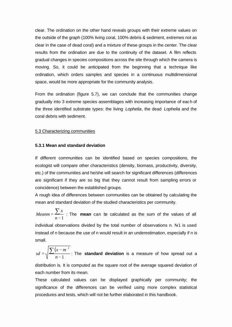
A rough idea of differences between communities can be obtained by calculating the

mean and standard deviation of the studied characteristics per community.

1−= ∑

n

xMeanµ : The mean can be calculated as the sum of the values of all

individual observations divided by the total number of observations n. N-1 is used

instead of n because the use of n would result in an underestimation, especially if n is

small.

( )1

2

−

−= ∑

n

xsd

µ: The standard deviation is a measure of how spread out a

distribution is. It is computed as the square root of the average squared deviation of

each number from its mean.

These calculated values can be displayed graphically per community; the

significance of the differences can be verified using more complex statistical

procedures and tests, which will not be further elaborated in this handbook.

5.3.2 Example of community characterization based on Haltenpipe data

The graph in figure 5.8 represents the variation in diversity between the three

communities that were defined in section 5.2.4. This graph indicates that the mean

diversity is the highest in the species community on dead coral (mean ES (100):

8.63) and the lowest in the species community on debris and sediment (mean ES

(100): 5.83). The community with living Lophelia shows an intermediate value (mean

ES (100): 6.55). These data confirm the statements of Mortensen (2000) and Jensen

& Frederiksen (1992) that the diversity is higher in areas of dead coral compared to

areas of living coral (see section 2.2.2), and that the reef shows a higher diversity

than the surrounding sediment (in this case, the sediment is mixed with debris).

The standard deviation gives an indication about the significance of these differences

in biodiversity: when there is a clear overlap between the whiskers, the difference will

probably be non-significant (e.g. between the diversities of the living coral community

and the debris/sediment community).

In this case, non-parametric statistical tests (Mann-Whitney U test and Kruskall-

Wallis test, for those who are familiar with statistical analyses) confirmed that the

difference between the dead coral community and the living coral community is

significant. That was also the case between the dead coral community and the

debris/sediment community but not between the living coral community and the

debris/sediment community.

Figure 5.8 Graph showing mean and standard deviation of the expected number of species per community. The squares represent the mean, the whiskers the standard error.

Mean+SD Mean-SD

Mean

Box Plot expected number of species

ES

__10

0_

3

5

7

9

11

dead

debris/sediment

Living coral coral

5.4 Indicator species and habitat preferences

5.4.1 Indicator species

A very common goal in community analysis is to detect and describe the value of

different species for indicating environmental conditions. These indicators can be

derived from data about the occurrence of species and from background information

about the environmental requirements of the species. The best indicators will be

those species with a narrow range of tolerance concerning a certain environmental

variable.

Example: Indicator species are a widely used tool to monitor the state of habitats

vulnerable to pollution (figure 5.9). Indicator species are species with a very low

tolerance for toxicants, turbidity of the water column or eutrophication. The presence

or absence of indicator species will tell you if the water is polluted or not, while this

information cannot be obtained from the presence of species with a very high

tolerance for pollution.

Species typically occurring in a certain community, which can possibly give an

indication about the environmental conditions, can be searched for with multivariate

analysis (see section 5.2).

Typical species for each community can be found in an ordination graph where the

species are plotted as points representing their optima of the response curve

concerning a certain environmental variable (example in section 5.4.2).

Another technique is called Indicator Species Analysis (Mc Cune & Mefford, 1999).

This method calculates the significance of an indicator by giving it a value between 0

(no indication) and 100 (perfect indication). Two factors are calculated:

Tolerance: response curve

0 20 40 60 80

100 120

0 50 100 150 200 concentration of polluting substance

num

ber

of in

divi

dual

s range

optimum

Figure 5.9 Example of response curve showing tolerance and range of occurrence in the presence of a polluting substance. The concentration that coincides with the highest number of individuals is the optimum.

# individuals of sensitive species # individuals of tolerant species

1. the proportional abundance of the species in a particular group relative to the

abundance of that species in all groups

2. the percentage of samples in each group that contain that species

Example: There are two sites with different environmental conditions; 4 samples

were taken at the first site and 2 samples were taken on the second site.

condition 1 condition 2 sample 1 sample 2 sample 3 sample 4 sample 1 sample 2

species 1 4 5 4 6 8 0 species 2 18 0 0 0 20 36

The first species will be a good indicator for the first environmental condition because

it has a higher abundance under that condition and the species is found in all

samples of the site, which is not the case the second site. Species 2 is a good

indicator for the other environmental condition.

Remark: The presence of an indicator species for a certain environmental variable in

a sample, does not necessarily give you an unequivocal indication about that

variable. If, for example, brittle stars would appear to be indicators for a substrate of

dead coral, it would be

impossible to say what substrate

the sample came from if you only

found one brittle star in your

sample. On the other hand, if

you found that brittle stars were

abundant and dominant in the

sample, then you could say that there is a large possibility that the sample came from

a site with a dead coral substrate.

See also exercise 6

5.4.2 Taxonomic and trophic organization

Community analysis is not always limited to the species level. The characterization of

the faunal communities can also be done on other levels: on a higher taxonomical

level, on the level of trophic organization (feeding types), on the types of locomotion,

etc. These data can give indications about the environmental settings additional to

those obtained from species data and they can provide insights in the functioning of

the different communities.

Figure 5.10 An ophiuroid (Ophiactis abyssicola) from the Porcupine Seabight (photo Kai Kaszemeik, from Van Gaever, 2001)

q Higher taxonomical level: Taxonomy is that field of science that

classifies life in well-defined groups and which is based on the species-

concept. Species are grouped into genera, families, orders, classes, and

phyla, depending upon similarities and inferred evolutionary relationships.

Example: The classification of the crab species Cancer pagurus (Hayward &

Ryland, 1996): Phylum Crustacea

Class Malacostraca

Order Decapoda

Family Cancridae

Genus Cancer

Species Cancer pagurus

The faunal composition of a community can be analyzed on each of these

levels. You can find a video fragment of Cancer pagurus (fragment 5) on the CD.

q Feeding types: Due to the absence of light in the deep-sea, there can

be no primary production from photosynthesis. Therefore, most of the

organisms depend on sinking surface material, mostly phytodetritus (the

remains of dead phytoplankton), faecal pellets and animal carcasses. A lot of

deep-sea animals are suspension feeders, meaning that they capture

particles suspended in the water (e.g.sponges and sabellid worms). Other

animals, the deposit feeders, ingest sediment and digest the nutritional

fraction. Typical examples are sea cucumbers and echiurid worms. A last

group of animals consists of the scavengers, which feed on carcasses, and

predators.

q Types of

locomotion: The deep-sea

megafauna includes both

mobile and sessile

organisms. The former

includes many

echinoderms, mollusks

(inclusing octopods), sea

spiders (pycnogonids), true

crabs, hermit crabs,

shrimps, squat lobsters and

the benthic fishes. The

sessile organisms include

Copyright IFREMER

Figure 5.11 Assemblage of sessile fauna from Theresa Mound, Ireland: little anemones, Lophelia pertusa and a gorgonian octocoral (probably Paramuricea placomus)

Copyright IFREMER

sponges, anemones, corals, sea lilies, barnacles, mussels and ascidians

(Herring, 2002)

5.4.3 Example based on Haltenpipe data

A. Indicator species

The ordination graph on figure 5.13 shows samples and

species simultaneously plotted against the ordination axes.

The position of the species points on the graph can be used

to define indicator species for each of the three

communities. In this case, the following species will probably

be indicators:

• Sebastes viviparus, the unidentified teleost (juvenile

Sebastes?) and the anemone Bolocera tuediae for

the species community on living Lophelia

• Pollachius virens for the species community on coral rubble and sediment

• 2 species of Sabellidae, ophiuroids, Hathrometra sarsi, Cidaris cidaris and

Munida sp. for the species community on dead coral. See Sebastes viviparus and Bolocera tuediae on video fragment 2 on the CD.

The significance of these species as indicators for the three communities was verified

with the technique of Indicator Species Analysis. Only three species seemed to be

significant indicators:

• Sebastes viviparus: highly significant indicator for the species community on

living Lophelia: 86% of the individuals were observed in association with living

Lophelia and 82% of the living coral samples contained Sebastes viviparus.

• Pollachius virens: highly significant indicator for the species community on

coral debris and sediment: 77% of the individuals was observed in

association with coral debris and sediment and all samples (100%) with

debris and sediment are characterized by the presence of saithe (Pollachius

virens).

• Cidaris cidaris: significant indicator for the species community on dead coral:

all individuals (100%) were found associated with dead coral and 33% of the

dead coral samples contained the species Cidaris cidaris.

These three species are indicators for environmental variables in the communities,

respectively for the coverage of the seafloor with living coral, dead coral and coral

Figure 5.12 Norway Redfish (Sebastes viviparus) from Haltenpipe, Norway

STATOIL

rubble plus sediment. Now it is possible to derive the substrate type from data on the

species composition (see exercises).

The species in the center of the graph, like Mycale lingua and Paragorgia arborea,

are common in all three communities. They are certainly not indicators.

B. Taxonomic and trophic organization

The following figures show differences in the amount of sessile and mobile fauna, the

amount of suspension feeders, deposit feeders, scavengers and predators, the

amount of individuals per higher taxon, and the amount of individuals in the 10 most

common species, per community.

1. Figure 5.14 shows the distribution of the relative abundances of the 10

most common species over the three communities.

Axis 1

Mycaling

Axinspec

sponspe4

Geodspec

sponspe6

sponspe8

Poeccomp

Hydrspec

Protsimp

Bolotued

PrimPara

Sabespe1

Sabepavo

Sabespe8

Acesexca

Decaspe

c

Munispec

Cidacida

Hathsars

Astespe1

Ophispec

Sebavivi

Brosbros

Pollvire

Telespec

Axi

s 2

Living coral

Dead coral

Debris & sediment

Figure 5.13 Ordination graph (CA) with samples and species scores. The position of the species can be used to define indicator species for each of the three communities

Paraarbo

The most obvious feature on this graph is the dominance of saithe (Pollachius

virens) and the sponge Mycale lingua in the community associated with debris

and sediment. The living coral community is characterized by Sebastes

viviparus, octocorals, the anemone Prothantea simplex and the sponge

Mycale lingua. The situation is similar in the dead coral community but the fish

Sebastes viviparus is less common.

2. Figure 5.15 shows that the species community associated with coral debris

and sediment is characterized by a higher percentage (mean 77.8%) of

mobile fauna compared to the other communities in which the majority of the

fauna are sessile.

Figure 5.15 Occurrence of mobile and sessile fauna

0% 20% 40% 60% 80%

100%

debris & sediment

Living coral

Dead coral

mea

n p

erce

nta

ge

mobile sessile

0%

20%

40%

60%

80%

100%

Dead coral

Living coral

debris & sediment

rest

Pollachius virens

Sebastes viviparus

Ophiuroidea spec

Hathrometra sarsi

Munida spec

Sabella pavonina

Paragorgia arborea

Primnoa resedaeformis & Paramuricea placomus

Protanthea simplex

Mycale lingua

Figure 5.14 Distribution of the mean relative abundances of the 10 most common species over the three substrate types

3. Figure 5.16 shows the distribution of the feeding types per community. The

living coral community and the dead coral community are again very similar

with 60-80% mean percentage of suspension feeders, while the community

associated with debris and sediment is characterized by almost 75% of

scavengers and predators. Deposit feeders (only Echiuroidea) are scarce.

4. Figure 5.17 shows the distribution of the relative abundance of higher taxa

over the communities. The distribution is different compared to those of the

separate species. In this case the communities on living Lophelia and coral

debris and sediment are the most similar. The dead coral community contains

less fish but more echinoderms and crustaceans.

C. Conclusion The community associated with living Lophelia is characterized by:

• The presence of the indicator species Sebastes viviparus

• Dominance of suspension feeders and sessile fauna

Figure 5.16 Feeding types

0%

20%

40%

60%

80%

100%

Dead coral

Living coral

debris & sediment

mea

n p

erce

nta

ge

scavengers & predators deposit feeders suspension feeders

Figure 5.17 Preferences of higher taxa

0%

20%

40%

60%

80%

100%

dead living debris & sediment

communities

mea

n p

erce

nta

ge

fish

echinoderms

crustaceans

molluscs

Echiuroids

polychaetes

cnidarians

spongescoral

coral

The community associated with dead Lophelia is characterized by:

• The presence of the indicator species Cidaris cidaris

• Dominance of suspension feeders and sessile fauna

• A low abundance of fish and a high abundance of echinoderms and

crustaceans

The community associated with coral debris and sediment is characterized by:

• The presence of the indicator species Pollachius virens

• Dominance of mobile fauna

• Dominance of scavengers and predators

6. Conclusions

The main objective of this handbook was to introduce the concepts of biodiversity

and community analysis to graduate and undergraduate students. The following list

gives an overview of things to remember from this handbook:

The sampling method is an essential element in ecological investigations.

Think carefully before you choose a sampling technique: make it as cheap as

possible but always keep the objectives of your study in mind. Minimize the

disturbance and bias of your samples and choose the sample size carefully.

Your samples must be representative for the studied species community. The

same goes for the measurement of environmental variables: make sure you

measure the most important structuring variables.

Nowadays, there is a large variety in biodiversity indices. When choosing an

index, you have to consider a lot of factors, especially the dependency on

sample size and the weight you want to give to rare or dominant species.

Community analysis is a complex process that can be facilitated using

multivariate and statistical analysis. But keep in mind that statistics are not the

goal in community analyses; they are only a medium to describe the variation

in species assemblages. After processing the data on species and their

abundances, also try looking at your data on other levels, like the level of

trophic organisation, the mobility of the species and higher taxonomical levels.

Another objective of this handbook was to acquaint you with cold-water coral

ecosystems. This was done using exercises and examples based on data from

Norwegian and Irish coral reefs. For those who want to know more or want to see

more beautiful pictures, the following list gives you a few interesting websites:

=> http://www.uni-tuebingen.de/geo/gpi/ag-freiwald/proj/aces/ : ACES project

=> http://www.geomar.de/projekte/ecomound/ecomoundstart: ECOMOUND

=> www.kystnett.no/~emil/skarnsundet/skarnsundet.htm : Trondheimsfjord

=> www.sams.ac.uk/dml/projects/benthic/lophns.htm : Lophelia on oil platforms

=> www.ukbap.org.uk/plans/habitats/NBNSYS0000004650.htm : protection

=> privat.egersund.com/erling/Nesledyr/page4.htm : pictures of species

=> www.pcweb.liv.ac.uk/ocean/org_geochem/aces.html: geochemistry

7. Glossary

ACES: Atlantic Coral Ecosystem Study, an international and multidisciplinary study

focussing on the cold- water corals from Galicia Bank, Spain (43°N), Porcupine

Seabight, Ireland (51°N), Rockall Trough, Ireland (59°N), Kosterfjord, Sweden (59°N)

and the Norwegian Shelf (64°N). This study is situated within the EC fifth framework

programme (1998-2002), just like Ecomound and Geomound. => http://www.uni-tuebingen.de/geo/gpi/ag-freiwald/proj/aces/

Benthic: ‘associated with the seafloor’ – benthic fauna include epibenthos (on the

seafloor), the infauna or endobenthos (in the sediment) and the benthopelagic fauna

(pelagic animals living in close association with the seafloor) (Herring, 2002).

CANOCO: for more information see

=> www.microcomputerpower.com/catalog/canoco.html

Clones: group of cells or organisms arising by asexual reproduction from a single

parent individual. Clones therefore have exactly the same genetic make-up (Lafferty

& Rowe, 1994)

Cnidocytes: stinging structures of cnidarians that are most abundant in tentacles. A

discharged cell consists of a capsule and a thread that can be armed with spines;

many cells can inject a toxin into the prey.

Deposit feeder: deposit feeders ingest sediment, selectively or not. The organic

portion is digested, the rest is eliminated.

ECOMOUND: Environmental Controls on Mound Formation along the European

Continental Margin. The objective of this programme is to define the environmental

controls and processes involved in the development and distribution of carbonate

mounds on the NW European continental margin.

=> http://www.geomar.de/projekte/ecomound/ecomoundstart

Words explained in glossary are underlined in the text

Eutrophication: a state of pollution resulting from introduction of sediments, sewage

or fertilizers into a waterway, causing an increase of the concentration of available

nutrients in that system.

Flagellum: small hairlike organelle on the surface of certain cells (e.g. single-celled

algae and sperm cells of higher animals). The movement of the flagellum can be

used for locomotion of the cell or to create water movements.

Gas hydrate: A gas hydrate is a crystalline solid similar to ice. Its building blocks

consist of a gas molecule surrounded by a cage of water molecules. Many gases

have molecular sizes suitable to form hydrate, including such naturally occurring

gases as carbon dioxide, hydrogen sulphide, and several low-carbon-number

hydrocarbons, but most marine gas hydrates that have been analysed are methane

hydrates.

GEOMOUND: This project focuses on the geological evolution of giant, deep-water

carbonate mounds in the Porcupine Basin and southeast Rockall Basin, off western

Ireland and the UK.

=> http://geomound.ucd.ie/

Lateral line system: system of sense organs in fishes that detects water movement.

It usually consists of a row of interconnected pores on either side of the body that

divide into a system of canals across the head.

Margin: boundary between coastal zone and open ocean, consists of the continental

shelf, slope and rise.

Normal distribution: important class of statistical distributions. All normal

distributions are symmetric and have bell-shaped density curves with a single peak.

The peak of the density coincides with the mean and the standard deviation

indicates the spread of the bell curve. In a normal distribution, 68% of the

observations fall within 1 standard deviation of the mean, that is, between and

.

PC-ORD: for more information see

=> www.ptinet.net/~mjm/pcordwin.htm

Pockmarks: craters developed in soft, fine-grained seafloor sediments by the action

of focused drainage of pore water and gases through the seafloor (Hovland & Judd,

1988)

Population: a group of individuals of one species in an area, though the size and

nature of the area is defined, often arbitrarily, for the purposes of the study being

undertaken (Begon et al, 1996)

Reef: In scientific literature, there has been some debate about the use of the term

‘reef’ for structures built by Lophelia, because Lophelia is an azooxanthellate coral.

Therefore, there are different terms for accumulations of azooxanthellate coral

colonies and skeletons: reef (e.g. Mortensen, 2000), massif (e.g. Le Danois, 1948),

bank (e.g. Jensen & Frederiksen, 1992), patch (e.g. Wilson, 1979), mound (e.g.

Hovland et al, 1994) and bioherm. In this handbook, the term ‘reef’ will be used.

Species: Groups of actually or potentially interbreeding natural populations which are

reproductively isolated from other such groups. May or may not be morphologically

distinct.

STATOIL: Statoil is a Norwegian company carrying out exploration, production,

transportation, refining and marketing of petroleum and petroleum-derived products.

Scleractinians: stony reef-building corals

Sessile: attached to a substrate, not mobile

Swimbladder: a hydrostatic organ used to obtain neutral buoyancy and facilitate

movement in the water column

Symbiosis: a close association between two species generally (with the exception of

parasitism) seeming to be unharmful to either member, or, more likely, beneficial to

one or both. Parasitism, commensalism, and mutualism are the three types of

symbiotic relationships.

Taxon (plural: taxa): unit of classification of living organisms (phylum, class, family,

genus, species)

Thermocline: the depth at which the temperature gradient is a maximum: generally a

layer of water with a more intensive vertical gradient in temperature than in the layers

either above or below it. It is an area of water within the water column in which the

warmer upper waters are prevented from mixing with those at a deeper level. This

barrier prevents the interchange of nutrients between the two.

Zooxanthellae: vegetative stadium of the dinoflagellate Gymnodium

microadriaticum, living inside the tissue of tropical corals. It provides oxygen

(promotes calcification), glucose and glycerol to the coral and uses nutrients

produced by the coral like nitrates, ureic acid and phosphates. These algae allow the

corals to grow faster.

8. References Barnett PRO, Watson J and Connely D (1984) A multiple corer for taking virtually undisturbed samples from shelf, bathyal and abyssal sediment. Oceanologica acta vol. 7(4) 399-408 Begon M, Harper JL & Townsend CR (1996) Ecology. Blackwell Science. 1068p.

Bett BJ, Vanreusel A., Vincx M, Soltwedel T, Pfannkuche O, Lambshead PJD, Gooday AJ, Ferrero T and Dinet A (1994) Sampler bias in the quantitative study of deep-sea meiobenthos. Mar. Ecol. Prog. Ser. Vol. 104: 197-203 Blomqvist S (1991) Quantitative sampling of soft-bottom sediments: problems and solutions. Mar. Ecol. Prog. Ser. Vol 72: 295-304 De Mol B, Van Rensbergen P, Pillen S, Van Herreweghe K, Van Rooij D, McDonell A, Huvenne V, Ivanov M, Swennen R & Henriet JP (in press) Large deep-water coral banks in the Porcupine Basin, southwest of Ireland. 42p Frederiksen R, Jensen A & Westerberg H (1992) The distribution of the scleractinian coral Lophelia pertusa around the Faroe islands and the relation to internal tidal mixing. Sarsia 77: 157-171 Freiwald A, Henrich R and Pätzold J (1997) Anatomy of a deep-water coral reef mound from Stjernsund, west Finnmark, northern Norway: in James NP & Clarke JAD eds., Cool-water Carbonates: Society of Sedimentary Geologists (SEPM), Special Publication, 56, p 140-161 Freiwald A (1998) Geobiology of Lophelia pertusa (Scleractinia) reefs in the North Atlantic. Habilitationsschrift zur Erlangung de venia legendi am Fachbereich Geowissenshaften der Universität Bremen, 116p Gage JD & Tyler PA (1996) Deep-sea biology. A natural history of organisms at the deep-sea floor. Cambridge University Press. 504p Gordon DC, Kenchington ELR, Gilkinson KD, McKeown DL, Steeves G, Chin-Yee M, Vass WP, Bentham K and Boudreau PR (2000) Canadian imaging and sampling technology for studying marine benthic habitat and biological communities. Ices 2000 Annual Science Conference. Gutt J & Starmans A (2001) Quantification of iceberg impact and benthic recolonisation patterns in the Weddell Sea (Antarctica). Polar Biology 24: 615-619 Hayward PJ & Ryland JS (1996) Handbook of the Marine Fauna of North-West Europe. Oxford University Press. 800p Heip CHR, Herman MJP & Soetaert K (1983) Indices of biodiversity and evenness. Océanis 24 (4) 61-87p Heip C, Herman PMJ and Soetaert K (1998) Indices of diversity and evenness. Océanis 24 (4): 61-87

Henriet JP, de Mol B, Pillen S, Vanneste M, Van Rooij D, Versteeg W, Croker PF, Shannon PM, Unnithan V, Bouriak S, Chachkine P & Porcupine-Belgica 97 Shipboard Party (1998) Gas hydrate crystals may help build reefs. Nature 391: 648-649 Herring P (2002) The Biology of the Deep Ocean. Oxford University Press. 314p Higgins RP & Thiel H (1988) Introduction to the study of meiofauna. Smithsonian Institution Press Washington/London. Hill MO (1973) Diversity and evenness: a unifying notation and its consequences. Ecology, 54: 427-432 Hovland M & Thomsen E (1997) Cold-water corals – are they hydrocarbon seep related? Marine Geology, 137: 159-164 Hovland M, Mortensen PH, Brattegard T, Strass P and Rokoengen K (1998) Ahermatypic Coral Banks off Mid-Norway: Evidence for a Link with Seepage of Light Hydrocarbons. Palaios, V.13 189-200p Hovland M & Mortensen PB (1999) Norske korallrev og processer i havbunnen. John Grieg Forlag. 155p Hovland M, Vasshus S, Indreeide A, Austdal L and Nilsen ∅ (in press) Mapping and

imaging deep-sea coral reefs off Norway, 1982-2000

Hurlbert SH (1971) The nonconcept of species diversity: a critique and alternative

parameters. Ecology vol. 52, 4: 577-586

Jensen A & Frederiksen R (1992) The fauna associated with the bank-forming deepwater coral Lophelia pertusa (Scleractinia) on the Faroe shelf. Sarsia 77: 53-63 Kenyon NH, Ivanov MI and Akhmetzanov AM (1998) Cold water carbonate mounds and sediment transport on the Northeast Atlantic margin. Preliminary results of the geological and geophysical investigations during the TTR-7 cruise of R/V Professor Logachev in co-operation with the CORSAIRES and ENAM2 Programmes July-August, 1997. Intergovernmental Oceanographic Commission Technical Series, 52. 179p. UNESCO, Paris, France. Kenyon NH, Akhmetzanov AM, Wheeler AJ, van Weering TCE, de Haas H and Ivanov MI (in press) Giant carbonate mud mounds in the southern Rockall Trough. Marine Geology. Lafferty P and J Rowe (1994) Dictionary of Science. The World of science from Big Bang to Biodiversity, Brockhampton Press, London: 678p Lambshead PJD, Platt HM & Shaw KM (1983) The detection of differences among assemblages of marine benthic species based on an assessment of dominance and diversity. Journal of Natural History, 17: 859-874 Larson R, Morang A and Gorman L (1997) Monitoring the coastal environment 2: sediment sampling and geotechnical methods. Journal of Coastal Research 13 (2) 308-330

Le Danois E (1948) Les profondeurs de la mer. Payot Paris: 303p Ludwig JA & Reynolds JF (1988) Statistical Ecology, a primer on methods and

computing. John Wiley & sons. 85-103p

Mc Cune B & Mefford MJ (1999) PC-ORD. Multivariate Analysis of Ecological data, Version 4. MjM Softawer Design, Gleneden Beach, Oregon, USA. 237p Mortensen, PB, Hovland m, Brattegard T & Farestveit R (1995) Deep-water bioherms of the scleractinian coral Lophelia pertusa (L.) at 64°N on the Norwegian Shelf: structure and associated megafauna. Sarsia 80: 145-158 Mortensen, PB (2000) Lophelia pertusa (Scleractinia) in Norwegian waters – distribution, growth and associated fauna. Thesis submitted in partial fulfilment of the requirements for the degree of Dr. scient. Department of Fisheries and Marine Biology, University of Bergen. Mortensen, PB; Hovland M, Fossa JH and Furevik D (in press) Distribution, abundance and size of Lophelia pertusa coral reefs in mid-Norway in relation to seabed characteristics. Raes M. (2001) Biodiversiteit van meio-epifauna geassocieerd met koudwaterkoralen van de Porcupine Seabight. Licentiaatsthesis Biologie, University of Ghent . 160p Rogers AD (1999) The biology of Lophelia pertusa (Linnaeus, 1758) and other deep-

water reef-forming corals and impacts from human activities. Internat. Rev.

Hydrobiol. 84: 315-406

Ruppert EE & Barnes RD (1994) Invertebrate Zoology sixth edition. Saunders

College Publishing: 1056p

Soetaert K & Heip C. (1990) Sample-size dependence of diversity indices and the

determination of sufficient sample size in high-diversity deep-sea environment.

Marine Ecology Progress Series vol. 59: 305-307

Starmans A, Gutt J and Arntz WE (1999) Mega-epibenthic communities in Arctic and Antarctic shelf areas. Marine Biology 135: 269-280 Stetson TR, Squires DF and Pratt RM (1962) Coral banks occurring in deep water on the Blake Plateau. American Museum of Natural History. Number 2114 Strömgren T (1971) Vertical and horizontal distribution of Lophelia pertusa (Linné) in Trondheimsfjorden on the West Coast of Norway. Kongelige Norske Videnskabers Selskabs Skrifter 6: 1-9

Tasker M, Bett B, Fossa JH, Grehan A, Gordon J, Hall-Spencer J, Lorance P, Mortensen P and Wheeler A (2001) Initial report of the study group on cold water corals in relation to fishing (draft). SGCOR, 12p Teichert C (1958) Cold- and deep-water coral banks. Bull. Am. Ass. Petrol. Geol. 42 (5): 1064-1082 Van Gaever S (2001) Gemeenschapsanalyse van macrofauna geassocieerd met koudwaterkoraalriffen in de NO Atlantische Oceaan. Licentiaatsthesis biologie, University of Ghent. 110p Vetter EW & Dayton PK (1998) Macrofaunal communities within and adjacent to a detritus-rich submarine canyon system. Deep-Sea Research II 45 p 25-54 Vetter EW & Dayton PK (1999) Organic enrichment by macrophyte detritus, and abundance patterns of megafaunal populations in submarine canyons. Mar. Ecol. Prog. Ser. Vol. 186: 137-148 Vorberg R & van Bernem K-H (1998) Application of underwater video and imaging sonar in ecological investigations in the subtidal zone of the Wadden Sea. Arch. Fish. Mar. Res.46 (3), p 195-203 Wilson JB (1979) The first recorded specimens of the deep-water coral Lophelia pertusa (Linnaeus, 1758) from British waters. Bull. Br. Mus. Nat. Hist. (Zool.) 36 (4): 209-215 Wilson JB (1979) The distribution of the coral Lophelia pertusa (L.) (L. prolifera (Pallas)) in the North-East Atlantic. J. Mar. Biol. Ass. U.K. 59, 149-164

a

Appendix The appendix contains the 2 datasets constructed with the observations from the STATOIL film from the Haltenpipe coral reefs:

1) The dataset with samples, species and their abundances (raw data): pages a - e

2) The dataset with the estimations of the percentage seafloor coverage with debris plus sediment, living Lophelia and dead coral: page f

b

1:00-2:00 3:00-4:00 4:00-5:00 5:00-6:00 6:00-7:00 7:00-8:00 8:00-9:00 9:00-10:00 10:00-11:00 11:00-12:00

Mycale lingua (sp1) 5.000 12.500 7.692 25.000 13.333 17.647 7.692 33.333 11.538 8.333

Haliclona sp. (sp2) 0.000 2.083 0.000 0.000 0.000 0.000 0.000 0.000 0.000 0.000 Axinella sp. (sp3) 5.000 0.000 30.769 0.000 0.000 0.000 0.000 0.000 0.000 0.000 unidentified sponge (sp4) 0.000 0.000 0.000 0.000 0.000 0.000 0.000 0.000 0.000 0.000 Geodiidae sp. (sp5) 0.000 0.000 0.000 0.000 0.000 0.000 0.000 0.000 0.000 0.000 unidentified sponge (sp6) 0.000 0.000 0.000 0.000 0.000 0.000 0.000 0.000 0.000 0.000 Stellatta sp. (sp7) 0.000 0.000 0.000 0.000 0.000 0.000 0.000 0.000 0.000 0.000 unidentified sponge (sp8 flat, white) 0.000 0.000 0.000 0.000 0.000 0.000 0.000 0.000 0.000 0.000 Poecillastra compressa (sp9) 0.000 0.000 7.692 0.000 0.000 0.000 0.000 0.000 0.000 0.000 Hydrozoa sp. 5.000 0.000 0.000 0.000 0.000 0.000 0.000 0.000 0.000 0.000 Prothantea simplex 0.000 22.917 0.000 0.000 26.667 35.294 26.923 0.000 19.231 0.000 Bolocera tuedia 5.000 2.083 0.000 0.000 0.000 0.000 0.000 0.000 0.000 16.667 Unidentified anthozoan (white) 5.000 0.000 0.000 0.000 0.000 0.000 0.000 0.000 0.000 0.000 Unidentified octocoral sp1(white) 0.000 0.000 0.000 0.000 0.000 0.000 0.000 0.000 0.000 0.000 Primnoa resedaeformis & Paramuricea placomus 0.000 12.500 0.000 0.000 46.667 14.706 3.846 0.000 38.462 41.667 Paragorgia arborea 5.000 6.250 0.000 0.000 6.667 11.765 7.692 0.000 0.000 0.000 Sabellidae sp1(small, blue) 0.000 0.000 0.000 0.000 6.667 0.000 0.000 0.000 0.000 0.000 Sabella cf. pavonina 0.000 0.000 0.000 0.000 0.000 0.000 0.000 0.000 0.000 0.000 Sabellidae sp2 (red) 0.000 0.000 0.000 0.000 0.000 0.000 0.000 0.000 0.000 0.000 unidentified echiurid 0.000 0.000 7.692 0.000 0.000 0.000 0.000 0.000 0.000 0.000 Acesta excavata 0.000 0.000 0.000 0.000 0.000 5.882 0.000 0.000 0.000 0.000 Cancer pagurus 0.000 0.000 0.000 0.000 0.000 0.000 0.000 0.000 0.000 0.000 unidentified crab 0.000 0.000 0.000 0.000 0.000 0.000 0.000 0.000 0.000 0.000 unidentified decapod 0.000 0.000 0.000 25.000 0.000 0.000 0.000 0.000 0.000 0.000 Munida sp. 0.000 2.083 23.077 0.000 0.000 0.000 3.846 0.000 0.000 0.000 Cidaris cidaris 10.000 0.000 0.000 0.000 0.000 0.000 0.000 0.000 0.000 0.000 Hathrometra sarsi 20.000 33.333 0.000 0.000 0.000 8.824 15.385 0.000 0.000 0.000 Unidentified Asteroid sp1 35.000 6.250 23.077 50.000 0.000 0.000 0.000 0.000 0.000 0.000 Unidentified Asteroid sp2 0.000 0.000 0.000 0.000 0.000 0.000 0.000 0.000 0.000 0.000 Unidentified Ophiuroid 0.000 0.000 0.000 0.000 0.000 2.941 26.923 0.000 0.000 0.000 Sebastes viviparus 0.000 0.000 0.000 0.000 0.000 2.941 7.692 66.667 30.769 33.333 Brosme brosme 5.000 0.000 0.000 0.000 0.000 0.000 0.000 0.000 0.000 0.000 Pollachius vi rens 0.000 0.000 0.000 0.000 0.000 0.000 0.000 0.000 0.000 0.000 Micromesistius potassou 0.000 0.000 0.000 0.000 0.000 0.000 0.000 0.000 0.000 0.000 unidentified teleost 0.000 0.000 0.000 0.000 0.000 0.000 0.000 0.000 0.000 0.000

c

12:00-13:00 13:00-14:00 14:00-15:00 15:00-16:00 16:00-17:00 17:00-18:00 18:00-19:00 19:00-20:00 20-00:21:00 21:00-22:00 22:00-23:00

Mycale lingua (sp1) 10.526 54.545 22.222 25.000 23.077 36.842 18.919 12.963 21.429 21.053 13.333

Haliclona sp. (sp2) 0.000 0.000 0.000 0.000 0.000 0.000 0.000 0.000 0.000 0.000 0.000 Axinella sp. (sp3) 0.000 0.000 0.000 0.000 0.000 0.000 0.000 0.000 0.000 0.000 0.000 unidentified sponge (sp4) 0.000 0.000 0.000 0.000 5.128 2.632 2.703 0.000 0.000 2.632 0.000 Geodiidae sp. (sp5) 0.000 0.000 0.000 0.000 0.000 0.000 0.000 0.000 2.381 2.632 0.000 unidentified sponge (sp6) 0.000 0.000 0.000 0.000 0.000 0.000 0.000 0.000 0.000 0.000 0.000 Stellatta sp. (sp7) 0.000 0.000 0.000 0.000 0.000 0.000 0.000 0.000 0.000 0.000 0.000 unidentified sponge (sp8 flat, white) 0.000 0.000 0.000 0.000 0.000 0.000 0.000 0.000 0.000 0.000 0.000 Poecillastra compressa (sp9) 0.000 0.000 0.000 0.000 0.000 0.000 0.000 0.000 0.000 0.000 0.000 Hydrozoa sp. 0.000 0.000 0.000 0.000 0.000 0.000 0.000 0.000 0.000 0.000 0.000 Prothantea simplex 21.053 22.727 35.556 12.500 30.769 31.579 43.243 64.815 35.714 10.526 23.333 Bolocera tuedia 5.263 0.000 0.000 0.000 0.000 2.632 0.000 0.000 0.000 0.000 0.000 Unidentified anthozoan (white) 0.000 0.000 0.000 0.000 0.000 0.000 0.000 0.000 0.000 0.000 0.000 Unidentified octocoral sp1(white) 0.000 0.000 0.000 0.000 0.000 0.000 0.000 0.000 0.000 0.000 0.000 Primnoa resedaeformis & Paramuricea placomus 5.263 4.545 6.667 31.250 23.077 2.632 0.000 7.407 30.952 26.316 20.000 Paragorgia arborea 0.000 0.000 0.000 0.000 5.128 5.263 0.000 1.852 2.381 10.526 3.333 Sabellidae sp1(small, blue) 26.316 0.000 0.000 0.000 0.000 0.000 0.000 0.000 0.000 0.000 0.000 Sabella cf. pavonina 0.000 0.000 0.000 6.250 0.000 7.895 5.405 0.000 0.000 0.000 0.000 Sabellidae sp2 (red) 0.000 0.000 0.000 0.000 0.000 0.000 0.000 0.000 0.000 0.000 0.000 unidentified echiurid 0.000 0.000 0.000 0.000 0.000 0.000 0.000 0.000 0.000 0.000 0.000 Acesta excavata 0.000 0.000 0.000 0.000 0.000 0.000 0.000 0.000 0.000 0.000 0.000 Cancer pagurus 0.000 0.000 0.000 0.000 0.000 0.000 0.000 0.000 0.000 0.000 0.000 unidentified crab 0.000 0.000 0.000 0.000 0.000 0.000 2.703 0.000 0.000 0.000 0.000 unidentified decapod 0.000 0.000 0.000 0.000 0.000 2.632 0.000 0.000 4.762 0.000 0.000 Munida sp. 15.789 9.091 4.444 18.750 0.000 2.632 0.000 5.556 0.000 0.000 0.000 Cidaris cidaris 0.000 0.000 2.222 0.000 2.564 2.632 2.703 0.000 0.000 5.263 0.000 Hathrometra sarsi 0.000 0.000 2.222 0.000 0.000 0.000 0.000 0.000 0.000 0.000 26.667 Unidentified Asteroid sp1 0.000 0.000 4.444 0.000 0.000 0.000 2.703 1.852 0.000 0.000 0.000 Unidentified Asteroid sp2 0.000 0.000 0.000 0.000 0.000 0.000 0.000 0.000 0.000 0.000 0.000 Unidentified Ophiuroid 10.526 0.000 20.000 6.250 0.000 2.632 18.919 3.704 0.000 2.632 0.000 Sebastes viviparus 5.263 4.545 2.222 0.000 2.564 0.000 0.000 0.000 0.000 2.632 3.333 Brosme brosme 0.000 0.000 0.000 0.000 2.564 0.000 2.703 1.852 2.381 0.000 0.000 Pollachius virens 0.000 0.000 0.000 0.000 0.000 0.000 0.000 0.000 0.000 5.263 10.000 Micromesistius potassou 0.000 4.545 0.000 0.000 0.000 0.000 0.000 0.000 0.000 2.632 0.000 unidentified teleost 0.000 0.000 0.000 0.000 5.128 0.000 0.000 0.000 0.000 7.895 0.000

d

23:00-24:00 24:00-25:00 25:00-26:00 26:00-27:00 27:00-28:00 28:00-29:00 29:00-30:00 30:00-31:00 31:00-32:00 32:00-33:00 33:00:34:00

Mycale lingua (sp1) 21.739 8.333 18.182 33.333 33.333 42.593 6.897 5.714 1.724 0.000 12.308

Haliclona sp. (sp2) 0.000 0.000 0.000 0.000 0.000 0.000 0.000 0.000 0.000 0.000 0.000 Axinella sp. (sp3) 4.348 0.000 0.000 0.000 0.000 0.000 0.000 0.000 0.000 0.000 3.077 unidentified sponge (sp4) 0.000 0.000 0.000 0.000 0.000 0.000 0.000 0.000 0.000 5.556 0.000 Geodiidae sp. (sp5) 0.000 0.000 0.000 0.000 0.000 0.000 0.000 0.000 0.000 0.000 0.000 unidentified sponge (sp6) 0.000 4.167 0.000 0.000 0.000 1.852 0.000 0.000 0.000 0.000 0.000 Stellatta sp. (sp7) 0.000 0.000 0.000 0.000 0.000 0.000 0.000 0.000 0.000 0.000 0.000 unidentified sponge (sp8 flat, white) 0.000 0.000 0.000 0.000 0.000 0.000 0.000 0.000 0.000 0.000 0.000 Poecillastra compressa (sp9) 0.000 0.000 0.000 0.000 0.000 0.000 0.000 0.000 0.000 0.000 0.000 Hydrozoa sp. 0.000 0.000 0.000 0.000 4.167 0.000 0.000 0.000 0.000 0.000 1.538 Prothantea simplex 13.043 8.333 22.727 5.556 4.167 0.000 0.000 0.000 0.000 0.000 10.769 Bolocera tuedia 0.000 0.000 0.000 0.000 0.000 1.852 0.000 0.000 0.000 0.000 0.000 Unidentified anthozoan (white) 0.000 0.000 0.000 0.000 0.000 0.000 0.000 0.000 0.000 0.000 0.000 Unidentified octocoral sp1(white) 0.000 0.000 0.000 0.000 0.000 0.000 0.000 0.000 0.000 0.000 0.000 Primnoa resedaeformis & Paramuricea placomus 4.348 12.500 9.091 11.111 0.000 3.704 0.000 0.000 0.000 0.000 13.846 Paragorgia arborea 0.000 0.000 0.000 11.111 0.000 3.704 1.724 2.857 1.724 5.556 3.077 Sabellidae sp1(small, blue) 0.000 0.000 0.000 0.000 0.000 0.000 0.000 0.000 0.000 0.000 0.000 Sabella cf. pavonina 0.000 33.333 0.000 0.000 0.000 0.000 0.000 0.000 0.000 0.000 3.077 Sabellidae sp2 (red) 0.000 0.000 4.545 5.556 0.000 0.000 0.000 0.000 0.000 0.000 0.000 unidentified echiurid 0.000 0.000 0.000 0.000 0.000 0.000 0.000 0.000 0.000 0.000 0.000 Acesta excavata 0.000 0.000 0.000 0.000 0.000 0.000 0.000 0.000 0.000 0.000 0.000 Cancer pagurus 0.000 0.000 0.000 0.000 0.000 0.000 0.000 0.000 0.000 0.000 0.000 unidentified crab 0.000 0.000 0.000 0.000 0.000 0.000 0.000 0.000 0.000 0.000 0.000 unidentified decapod 0.000 0.000 0.000 0.000 0.000 0.000 0.000 0.000 0.000 0.000 0.000 Munida sp. 4.348 0.000 0.000 0.000 0.000 1.852 5.172 11.429 1.724 0.000 1.538 Cidaris cidaris 0.000 0.000 0.000 0.000 0.000 0.000 0.000 0.000 0.000 0.000 0.000 Hathrometra sarsi 0.000 12.500 4.545 0.000 4.167 1.852 0.000 0.000 0.000 0.000 3.077 Unidentified Asteroid sp1 0.000 0.000 0.000 0.000 0.000 0.000 1.724 2.857 1.724 0.000 0.000 Unidentified Asteroid sp2 0.000 0.000 0.000 11.111 0.000 0.000 0.000 0.000 0.000 0.000 0.000 Unidentified Ophiuroid 0.000 0.000 22.727 0.000 0.000 0.000 6.897 0.000 0.000 0.000 0.000 Sebastes viviparus 43.478 12.500 0.000 5.556 0.000 0.000 0.000 0.000 0.000 0.000 0.000 Brosme brosme 4.348 0.000 0.000 0.000 4.167 0.000 0.000 0.000 3.448 0.000 0.000 Pollachius virens 0.000 8.333 18.182 16.667 50.000 42.593 75.862 74.286 89.655 88.889 47.692 Micromesistius potassou 0.000 0.000 0.000 0.000 0.000 0.000 1.724 2.857 0.000 0.000 0.000 unidentified teleost 4.348 0.000 0.000 0.000 0.000 0.000 0.000 0.000 0.000 0.000 0.000

e

34:00-35:00 35:00-36:00 36:00-37:00 37:00-38:00 38:00-39:00 39:00-40:00 40:00-41:00 41:00-42:00 42:00-43:00 43:00-44:00 44:00-45:00

Mycale lingua (sp1) 18.605 28.000 9.091 19.355 15.625 24.324 1.695 12.500 50.000 23.810 8.333

Haliclona sp. (sp2) 0.000 0.000 0.000 0.000 0.000 0.000 0.000 0.000 0.000 0.000 0.000 Axinella sp. (sp3) 0.000 0.000 0.000 3.226 0.000 2.703 0.000 0.000 0.000 0.000 4.167 unidentified sponge (sp4) 2.326 0.000 0.000 0.000 0.000 0.000 0.000 0.000 0.000 0.000 0.000 Geodiidae sp. (sp5) 0.000 0.000 0.000 0.000 0.000 0.000 0.000 0.000 0.000 0.000 0.000 unidentified sponge (sp6) 0.000 0.000 0.000 3.226 0.000 0.000 0.000 0.000 0.000 0.000 4.167 Stellatta sp. (sp7) 0.000 0.000 0.000 0.000 0.000 5.405 0.000 0.000 0.000 0.000 0.000 unidentified sponge (sp8 flat, white) 0.000 0.000 0.000 0.000 0.000 0.000 1.695 6.250 0.000 0.000 0.000 Poecillastra compressa (sp9) 0.000 0.000 0.000 0.000 0.000 0.000 0.000 0.000 0.000 0.000 0.000 Hydrozoa sp. 0.000 0.000 3.030 0.000 0.000 0.000 0.000 0.000 0.000 0.000 4.167 Prothantea simplex 16.279 6.000 24.242 29.032 18.750 5.405 13.559 6.250 18.750 23.810 29.167 Bolocera tuedia 0.000 0.000 0.000 0.000 0.000 0.000 0.000 0.000 0.000 4.762 0.000 Unidentified anthozoan (white) 0.000 0.000 0.000 0.000 0.000 0.000 0.000 0.000 0.000 0.000 0.000 Unidentified octocoral sp1(white) 0.000 0.000 0.000 0.000 3.125 0.000 0.000 0.000 0.000 0.000 0.000 Primnoa resedaeformis & Paramuricea placomus 27.907 34.000 48.485 0.000 0.000 13.514 0.000 0.000 0.000 0.000 0.000 Paragorgia arborea 4.651 4.000 3.030 0.000 0.000 2.703 0.000 0.000 0.000 4.762 8.333 Sabellidae sp1(small, blue) 0.000 0.000 0.000 0.000 6.250 0.000 0.000 0.000 0.000 0.000 0.000 Sabella cf. pavonina 6.977 0.000 0.000 3.226 0.000 0.000 0.000 0.000 0.000 0.000 0.000 Sabellidae sp2 (red) 0.000 0.000 0.000 0.000 0.000 0.000 0.000 6.250 0.000 0.000 4.167 unidentified echiurid 0.000 0.000 0.000 0.000 0.000 0.000 0.000 0.000 0.000 0.000 0.000 Acesta excavata 2.326 2.000 0.000 0.000 0.000 0.000 0.000 0.000 0.000 0.000 0.000 Cancer pagurus 0.000 0.000 0.000 0.000 0.000 0.000 0.000 0.000 0.000 0.000 0.000 unidentified crab 0.000 0.000 0.000 0.000 0.000 0.000 0.000 0.000 0.000 0.000 0.000 unidentified decapod 0.000 0.000 0.000 0.000 0.000 0.000 0.000 0.000 0.000 0.000 0.000 Munida sp. 0.000 0.000 0.000 12.903 9.375 0.000 0.000 18.750 6.250 0.000 0.000 Cidaris cidaris 0.000 0.000 0.000 0.000 0.000 2.703 0.000 6.250 0.000 0.000 0.000 Hathrometra sarsi 2.326 0.000 0.000 0.000 0.000 0.000 0.000 18.750 6.250 0.000 4.167 Unidentified Asteroid sp1 0.000 0.000 0.000 0.000 0.000 0.000 1.695 0.000 0.000 0.000 0.000 Unidentified Asteroid sp2 0.000 0.000 0.000 0.000 0.000 0.000 0.000 0.000 0.000 0.000 0.000 Unidentified Ophiuroid 0.000 0.000 0.000 0.000 43.750 0.000 1.695 18.750 0.000 0.000 0.000 Sebastes viviparus 0.000 2.000 9.091 3.226 3.125 5.405 0.000 6.250 6.250 0.000 12.500 Brosme brosme 0.000 4.000 3.030 6.452 0.000 2.703 0.000 0.000 0.000 0.000 0.000 Pollachius virens 18.605 20.000 0.000 19.355 0.000 35.135 79.661 0.000 12.500 42.857 20.833 Micromesistius potassou 0.000 0.000 0.000 0.000 0.000 0.000 0.000 0.000 0.000 0.000 0.000 unidentified teleost 0.000 0.000 0.000 0.000 0.000 0.000 0.000 0.000 0.000 0.000 0.000

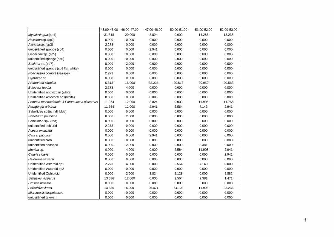
f

45:00-46:00 46:00-47:00 47:00-48:00 50:00-51:00 51:00-52:00 52:00-53:00

Mycale lingua (sp1) 31.818 20.000 8.824 0.000 14.286 13.235

Haliclona sp. (sp2) 0.000 0.000 0.000 0.000 0.000 0.000 Axinella sp. (sp3) 2.273 0.000 0.000 0.000 0.000 0.000 unidentified sponge (sp4) 0.000 0.000 2.941 0.000 0.000 0.000 Geodiidae sp. (sp5) 0.000 0.000 0.000 0.000 0.000 0.000 unidentified sponge (sp6) 0.000 0.000 0.000 0.000 0.000 0.000 Stellatta sp. (sp7) 0.000 2.000 0.000 0.000 0.000 0.000 unidentified sponge (sp8 flat, white) 0.000 0.000 0.000 0.000 0.000 0.000 Poecillastra compressa (sp9) 2.273 0.000 0.000 0.000 0.000 0.000 Hydrozoa sp. 0.000 0.000 0.000 0.000 0.000 0.000 Prothantea simplex 6.818 18.000 38.235 20.513 30.952 20.588 Bolocera tuedia 2.273 4.000 0.000 0.000 0.000 0.000 Unidentified anthozoan (white) 0.000 0.000 0.000 0.000 0.000 0.000 Unidentified octocoral sp1(white) 0.000 0.000 0.000 0.000 0.000 0.000 Primnoa resedaeformis & Paramuricea placomus 11.364 12.000 8.824 0.000 11.905 11.765 Paragorgia arborea 11.364 12.000 2.941 2.564 7.143 2.941 Sabellidae sp1(small, blue) 0.000 0.000 0.000 0.000 0.000 0.000 Sabella cf. pavonina 0.000 2.000 0.000 0.000 0.000 0.000 Sabellidae sp2 (red) 0.000 0.000 0.000 0.000 0.000 0.000 unidentified echiurid 2.273 0.000 0.000 0.000 0.000 0.000 Acesta excavata 0.000 0.000 0.000 0.000 0.000 0.000 Cancer pagurus 0.000 0.000 2.941 0.000 0.000 0.000 unidentified crab 0.000 0.000 0.000 0.000 0.000 0.000 unidentified decapod 0.000 2.000 0.000 0.000 2.381 0.000 Munida sp. 0.000 4.000 0.000 2.564 11.905 2.941 Cidaris cidaris 0.000 0.000 0.000 0.000 0.000 2.941 Hathrometra sarsi 0.000 0.000 0.000 0.000 0.000 0.000 Unidentified Asteroid sp1 2.273 4.000 0.000 2.564 7.143 0.000 Unidentified Asteroid sp2 0.000 0.000 0.000 0.000 0.000 0.000 Unidentified Ophiuroid 0.000 2.000 8.824 5.128 0.000 5.882 Sebastes viviparus 13.636 12.000 0.000 2.564 2.381 1.471 Brosme brosme 0.000 0.000 0.000 0.000 0.000 0.000 Pollachius virens 13.636 6.000 26.471 64.103 11.905 38.235 Micromesistius potassou 0.000 0.000 0.000 0.000 0.000 0.000 unidentified teleost 0.000 0.000 0.000 0.000 0.000 0.000

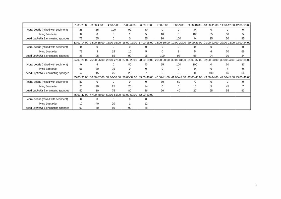
g

1:00-2:00 3:00-4:00 4:00-5:00 5:00-6:00 6:00-7:00 7:00-8:00 8:00-9:00 9:00-10:00 10:00-11:00 11:00-12:00 12:00-13:00

coral debris (mixed with sediment) 25 35 100 99 40 0 0 0 0 0 0

living Lophelia 0 0 0 1 5 10 0 100 85 50 5

dead Lophelia & encrusting sponges 75 65 0 0 55 90 100 0 15 50 95

13:00-14:00 14:00-15:00 15:00-16:00 16:00-17:00 17:00-18:00 18:00-19:00 19:00-20:00 20-00:21:00 21:00-22:00 22:00-23:00 23:00-24:00

coral debris (mixed with sediment) 0 0 0 0 0 0 0 0 0 0 0

living Lophelia 75 3 15 10 5 0 8 5 6 70 66

dead Lophelia & encrusting sponges 25 95 85 90 95 100 92 95 94 30 34

24:00-25:00 25:00-26:00 26:00-27:00 27:00-28:00 28:00-29:00 29:00-30:00 30:00-31:00 31:00-32:00 32:00-33:00 33:00:34:00 34:00-35:00

coral debris (mixed with sediment) 0 5 0 80 93 95 100 100 0 30 33

living Lophelia 96 80 75 0 0 0 0 0 0 4 0

dead Lophelia & encrusting sponges 4 15 25 20 7 5 0 0 100 66 66

35:00-36:00 36:00-37:00 37:00-38:00 38:00-39:00 39:00-40:00 40:00-41:00 41:00-42:00 42:00-43:00 43:00-44:00 44:00-45:00 45:00-46:00

coral debris (mixed with sediment) 30 0 0 0 0 80 60 70 0 0 0

living Lophelia 20 90 25 20 14 0 0 10 5 45 7

dead Lophelia & encrusting sponges 50 10 75 80 86 20 40 20 95 55 93

46:00-47:00 47:00-48:00 50:00-51:00 51:00-52:00 52:00-53:00

coral debris (mixed with sediment) 0 0 0 0 0

living Lophelia 10 40 20 1 12

dead Lophelia & encrusting sponges 90 60 80 99 88

Exercise 1

Below, you will find some objectives of ecological investigations concerning deep-sea

ecosystems. The aim of this exercise is that you try to find the most appropriate

sampling technique.

A. You have found a site that used to be covered with Lophelia pertusa and its

associated fauna but now it is heavily damaged due to intensive trawling. You would

like to monitor the changes in megafauna on this particular site to determine whether

the ecosystem can recover from this damage or not. What sampling method or

device would you use?

1. Dredge sampler

2. ROV with video equipment

3. Bathysnap

B. You would like to study the meiobenthos (animals between 38 µm and 1mm of

size, living in the sediment) in the sediment around Lophelia reefs. What sampling

method or device would you use?

1. Video recordings

2. Multicorer

3. Grab sampler

C. Your research team has discovered a mound-like feature during a side-scan sonar

survey of the seafloor. You suspect that there is some Lophelia on top of it, but of

course you have to verify that by taking a seafloor sample. What sampling method or

device would you use?

1. Dredge

2. TV-grab

3. ROV with video equipment

Solutions exercise 1

A. 1. No, you are wrong! A dredge is just as damaging as a trawl so it is

certainly not appropriate to use this device to study the possible recovery of a

damaged site.

2. No, you are wrong! Monitoring is a long-term project that requires regular

observations of the site. An ROV is very expensive and it would cost you a lot

of money to lower the ROV every month for only a few hours.

3. Yes, you are right! The Bathysnap device can be put on the seafloor for a

long period of time and it takes pictures at regular intervals. It is less

expensive than an ROV.

B. 1. No, you are wrong! Video material can only be used to observe large

animals living on top of the sediment, the so-called mega-epibenthos.

2. Yes, you are right! The multicorer can take up to nine small sediment

samples at the same time. These samples are virtually undisturbed and have

an intact upper layer, which is an important habitat for meiobenthic fauna.

3. No, you are wrong! A grab sampler takes large sediment samples, which is

unnecessary for meiobenthic studies. The samples are more disturbed and

you can only take one sample at the same time. It would save you a lot of

time if you used a multicorer.

C. 1. No, you are wrong! A dredge has been used frequently for this purpose in

the past, but this device is very damaging. As a good ecologist with a lot of

respect for the wonders of nature, you will choose an alternative sampling

method.

2. Yes, you are right! A TV-grab allows you to trace the corals first, after

which you can take a sample.

3. No, you are wrong! An ROV would be more suited if you would want to

map the coral reef and investigate zonation patterns.

Exercise 1

Imagine 2 samples, each containing 10 species and 100 individuals. In sample 1

(blue), every species occurred with 10 individuals while there was one species with

91 individuals in sample 2 (pink). The other 9 species occurred with only one

individual.

Sp.1 Sp.2 Sp.3 Sp.4 Sp.5 Sp.6 Sp.7 Sp.8 Sp.9 Sp.10

Sample 1 10 10 10 10 10 10 10 10 10 10

Sample 2 91 1 1 1 1 1 1 1 1 1

table 1. Two samples, each are containing 10 species (sp.), with indication of the

abundance of the species in each sample.

SR.1 SR.2 SR.3 SR.4 SR.5 SR.6 SR.7 SR.8 SR.9 SR.10

Sample 1 10 20 30 40 50 60 70 80 90 100

Sample 2 91 92 93 94 95 96 97 98 99 100

table 2. The same two samples, each containing 100 individuals. The species are

ranked according to their abundance and the cumulative abundance of all individuals

within each sample is calculated.

Question:

What sample has the highest diversity?

A. Sample 1

B. Sample 2

Figure 4.4. represents the graph of the cumulative frequencies (%) of the species in two samples.

number of species and evenness

0

20

40

60

80

100

120

1 2 3 4 5 6 7 8 9 10 11

species rank

cum

ula

tive

fre

qu

ency

Solution:

A. That is correct: Although both samples are characterized by the same

number of species, they display a different distribution of the individuals over

the species. Species 1 in sample 2 is clearly dominant, while all individuals in

sample 1 are equally spread over the species: high evenness.

B. That is not correct. The cumulative frequency curve indicates that sample 2 is

clearly dominated by one or more species, indicating a lower evenness than

sample 1.

Exercise 2

As already mentioned, photographs and video images were used to build up this

handbook. These images are not standardised, so every picture covers a different

surface on the seafloor (e.g. figure 4.5).

Question:

When you would want to compare the diversity between the species assemblages in

the pictures, what diversity indices do you think would be appropriate?

a) Shannon-Wiener index

b) Hill’s diversity numbers

c) Rarefaction

Answer:

a) You are partly right. Although the Shannon-Wiener index is sample size-

dependent, it can be a useful index if you want to compare with literature

concerning Lophelia and its associated fauna.

Figure 4.5 Pictures from Theresa Mound, representing different surfaces of the seafloor.

Copyright IFREMER Copyright IFREMER

b) You are partly right. The dominance index N∞ can be used in the case of

variable sample sizes but this is not true for N0 and N1

c) You are right. Rarefaction allows comparing samples in terms of number of

species; it is not correlated with sample size.

Exercise 3

The following picture was taken in one of the Haltenpipe coral reefs in Norway. The

lower part of the picture shows coral rubble, while the upper part shows dead coral

framework. The aim of this exercise is to calculate the species richness, diversity

(Shannon-Wiener index) and evenness.

The following table contains the species recognised in this picture and the number of

individuals per species. You can try to find these species back in the picture (if you

cannot see them on this picture, try examining the digital picture on the CD-rom using

a zoom function). Disregard the encrusting yellow and blue sponges; it is impossible

to quantify them because individual sponges are hard to discern. They can be

regarded as part of the substrate (! this means you will underestimate diversity!). For

this exercise you will need a calculator or a spreadsheet!

STATOIL

Notations:

Pi = the number of individuals of a given species divided by the total number of

organisms

S = the number of species in the picture

Shannon-Wiener index: H’ = -sum(Piln[Pi])

Evennes: J = H’/ ln S

Now calculate the values in the columns and make the sum of each column. The

negative value of the sum of the Pi ln Pi values will give you the Shannon-Wiener

index. The quotient of the Shannon-Wiener index and ln S will give you the

evenness.

Species Name # ind. Pi Pi ln Pi

Munida sp. 3 Prothantea simplex 2

Ophiuroidea sp. 5 Sabella pavonina 2

Asteroidea sp. 1 Fish (probably Sebastes

viviparus) 1

∑

The final result should look like this:

Species Name # ind. Pi Pi ln Pi

Munida sp. 3 0.214286 -0.3301 Prothantea simplex 2 0.142857 -0.27799

Ophiuroidea sp. 5 0.357143 -0.36772 Sabella pavonina 2 0.142857 -0.27799

Asteroidea sp. 1 0.071429 -0.1885 Fish (probably Sebastes

viviparus) 1

0.071429 -0.1885 ∑ 14 1 -1.6308

Note the high evenness, which is an important contributor to the high biodiversity

found associated with cold-water coral reefs! The evenness is high because the

individuals are evenly spread over the species; there is no clearly dominant species.

S = Ln S = H’ = J =

S = 6 Ln S = 1.79 H’ = 1.63 J = 0.91

Exercise 4 The idea of this exercise is to make the concept of sample-size dependency clear to you.

The exercise is based on a photo taken on Theresa Mound, Ireland, during the CARACOLE

cruise of the summer of 2001. During this campaign, images were made with cameras

mounted on ROV Victor, from which you can see a part on the right side of the complete

photo (3).

Below you can see three pictures: (1) a small part of the photo, (2) a larger part of the photo

and (3) the complete photo. Calculate the Shannon-Wiener diversity index for each picture

using the method demonstrated in the previous exercise. You will have to make a matrix with

species and abundances per picture. Disregard encrusting sponges; colonies of octocorals

can be regarded as one individual. Compare the indices you have calculated and answer the

following question: is the Shannon-Wiener index influenced by sample-size?

i

Species Name # individuals Pi pilnpi

? ? ? ? ? ? ? ? ? ? ? ? ? ? ? ? S ? ? ?

1

Copyright IFREMER

Shannon-Wiener index picture 1,2 and 3 = ?

a

b

c

d

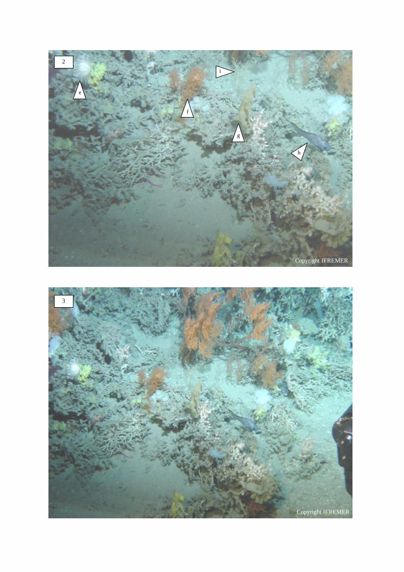
3

Copyright IFREMER

2

Copyright IFREMER

e

f

g

h

i

Solution Picture 1

Species Name # individuals Anemone sp. 2 Munida sp. 1 Sponge sp. (yellow) 1 Aphrocallistes bocasei 1

Picture 2

Species Name # individuals Anemone sp. 2 Munida sp. 1 Sponge sp. (yellow) 2 Aphrocallistes bocasei 4 Echinus sp. 1 Octocoral sp1 (orange) 3 Octocoral sp2 (yellow) 1 Fish sp. 1 Hydrozoa sp. 1

Picture 3

Species Name # individuals Anemone sp. (a) 2 Munida sp.(b) 1 Sponge sp. (yellow: c) 4 Aphrocallistes bocasei (d) 8 Echinus sp. (e) 1 Octocoral sp1 (orange: f) 4 Octocoral sp2 (yellow: g) 1 Fish sp. (h) 2 Hydrozoa sp. (i) 1

Is the Shannon-Wiener index influenced by sample-size?

Yes. The difference is very clear between de indices of picture 1 and 2, where 5 additional

species were found. The indices are almost the same between picture 2 and 3 because no

new species were found, only additional individuals of the already known species.

Remark

This exercise also tells you something about the best sample size for biodiversity studies

about this coral reef. Picture 1 only sampled one patch or microhabitat (see 4.2.1) of the

coral reef, which contains a limited number of species. However, when studying the diversity

of the complete coral reef, you have to sample all the different patches to get a complete

view of the biodiversity. That is why more small samples or bigger samples have to be taken.

In this case, a good sample size is represented by picture 2: the sample is large enough to

sample all species. Larger samples will only yield more individuals of the same species.

Shannon-Wiener index = 1.33

Shannon-Wiener index = 2.04

Shannon-Wiener index = 1.91

Exercise 5 On this picture from Theresa Mound, Ireland, you can recognize the following species:

species abundance Cidaris cidaris (a) 2 Echinus sp. (b) 2 Octocorallia sp. (c) 1 Aphrocallistes bocasei (d) 24 Yellow sponge (dead A. bocasei??) (e) 3

The aim of this exercise is to calculate the Hill-numbers for this sample (the photo). The

principle is the same as in exercise 3.

Species Name # ind. Pi ln Pi Pi ln P i Pi * Pi

Cidaris cidaris 2 Echinus sp. 2

Octocorallia sp. 1 Aphrocallistes bocasei 24 Yellow sponge (dead

A. bocasei??) 3

∑

With these values you can calculate the Hill-numbers as:

N0 = the number of species in the sample

Copyright IFREMER

d

b

a

c

e

N1 = the reciprocal of the Shannon-Wiener index = exp (-sum pilnpi)

N2 = the reciprocal of Simpson’s diversity index = 1/ (sum pi*pi)

N∞ = 1/pi of the most dominant species

The result should look like this:

Species Name # ind. Pi ln Pi Pi ln P i Pi * Pi

Cidaris cidaris 2 0.0625 -2.77259 -0.17329 0.003906 Echinus sp. 2 0.0625 -2.77259 -0.17329 0.003906 Octocorallia sp. 1 0.03125 -3.46574 -0.1083 0.000977 Aphrocallistes bocasei 24 0.75 -0.28768 -0.21576 0.5625 Yellow sponge (dead A. bocasei??) 3 0.09375 -2.36712 -0.22192 0.008789 ∑ 32 1 -11.6657 -0.89256 0.580078

With N0 = 5 N1 = 2.44 N2 = 1.72 N∞ = 1.33

Exercise 1 Suppose that you are working on a comparison between the species assemblages of cold-

water coral reefs from different sites in the Northeast-Atlantic. You have at your disposal data

of species abundances obtained from boxcore-samples at each site on these maps:

You could apply multivariate analysis in order to define groups of sites with similar species

assemblages. But what kind of multivariate analysis would you use?

a. classification

b. ordination

c. both

Solution:

c. It is recommended to use both techniques. The data will probably be discontinuous as

samples are taken from different sites with different environmental variables. There can

however, be gradients you are unaware of and those will not appear on a classification

dendrogram. It will be clear from both dendrogram and ordination if your data are

discontinuous. However, a gradient will only be visible on an ordination graph.

54°

56°

58°

60°

62°

64°

66°

68°

70°

5 °

5 °

10°

10°

15°

15°

20°

20°

25°

25°

Kosterfjord

Sula Ridge

35°

40°

45°

50°

-30°

-30°

-25°

-25°

-20°

-20°

-15°

-15°

-10°

-10°

-5°

-5°

0°

0°

Rockall Trough

Porcupine Slope

Galicia Bank

Figure 5.18 Five important cold-water coral areas in the Atlantic Ocean.

Exercise 2

The aim of this exercise is to make your own cluster dendrogram, starting from a simple data

matrix. For a cluster analysis, the following steps need to be followed (check every step with

the solutions before you proceed to the next!):

1. Create your data matrix with samples (first row), species (first column) and their

abundances (matrix entries)

29:00-30:00

9:00-10:00

18:00-19:00

20:00-21:00

24:00-25:00

30:00-31:00

Mycale lingua (sp1) 4 3 7 9 2 2 unidentified sponge (sp4) 0 0 1 0 0 0 Geodiidae sp. (sp5) 0 0 0 1 0 0 unidentified sponge (sp6) 0 0 0 0 1 0 Hymedesmia sp (sp10) 1 0 0 0 0 1 Prothantea simplex 0 0 16 15 2 0 Primnoa resedaeformis & Paramuricea placomus 0 0 0 13 3 0 Paragorgia arborea 1 0 0 1 0 1 Sabella cf. pavonina 0 0 2 0 8 0 unidentified crab 0 0 1 0 0 0 unidentified decapod 0 0 0 2 0 0 Munida sp. 3 0 0 0 0 4 Cidaris cidaris 0 0 1 0 0 0 Hathrometra sarsi 0 0 0 0 3 0 Unidentified Asteroid sp1 1 0 1 0 0 1 Unidentified Ophiuroid 4 0 7 0 0 0 Sebastes viviparus 0 6 0 0 3 0 Brosme brosme 0 0 1 1 0 0 Pollachius virens 44 0 0 0 2 26 Micromesistius potassou 1 0 0 0 0 1

number of species 8 2 9 7 8 7

Table 1. This matrix contains 6 samples from the Statoil film recorded on the Haltenpipe A reef.

It will be the basis of your cluster dendrogram.

2. Calculate the distance between all samples. Store the results in a distance matrix

The distance between samples can be expressed as a similarity index. For this

exercise, you can use the Sørensen index:

cda

Ss += with

The principle of the Sørensen index is as follows: the index only takes into account

presence or absence of species in the samples (so you don’t really need the

a = the number of common species in sample 1 and 2 b = the total number of species in sample 1 c = the total number of species in sample 2

abundances: you can replace the numbers in the matrix by zeros and ones if you

want). The more absences and presences of species two samples have in common,

the higher the index will become.

Example: similarity between the samples 29:00-30:00 and 9:00-10:00

cd

aSs +

= = 1/(8+2) = 0.1 now fill out the rest of the distance matrix

29:00-30:00 9:00-10:00 18:00-19:00 20:00-21:00 24:00-25:00 30:00-31:00

29:00-30:00 / 0.1 ? ? ? ? 9:00-10:00 / / ? ? ? ? 18:00-19:00 / / / ? ? ? 20:00-21:00 / / / / ? ? 24:00-25:00 / / / / / ? 30:00-31:00 / / / / / /

Table 2. Distance matrix with Sørensen indices

3. Search through the distance matrix and find the two most similar samples. Fuse these

two samples to produce a cluster.

ð These 2 samples will form your first cluster

ð

4. Calculate the distances between this new cluster and all other clusters/samples

These distances can be calculated using the Flexible Sorting method:

ijhjjhiihk dddd βαα ++=

with h, i and j: groups (samples) with nh, ni and nj elements (species)

dhi, dhj and dij: similarity indices between samples

k: cluster formed with samples i and j

dhk: similarity between new cluster and sample h

a = 0.625 and ß = -0.25

Try this yourself. If you don’t know how to do it, there is an example in the solutions.

5. Repeat until all samples are in one cluster

In the case of 2 identical distances: select the samples with the least similarity with

other samples/clusters.

Sample 1

Sample 2

6. What can you conclude from the cluster?

ð Can you discern communities? If so, how many and can you discuss them if

you know that: 9:00-10:00 = 100% living coral 29:00-30:00 = 95% debris and sediment

24:00-25:00 = 96% living coral 20-00:21:00 = 95% dead coral

30:00-31:00 = 100% debris and sediment 18:00-19:00 = 100% dead coral

Solution of exercise 1

Calculate the distance between all samples. Store the results in a distance matrix:

29:00-30:00 9:00-10:00 18:00-19:00 20:00-21:00 24:00-25:00 30:00-31:00

29:00-30:00 / 0.1 0.18 0.13 0.125 0.47 9:00-10:00 / / 0.09 0.11 0.2 0.11 18:00-19:00 / / / 0.19 0.18 0.125 20:00-21:00 / / / / 0.2 0.14 24:00-25:00 / / / / / 0.13 30:00-31:00 / / / / / /

Search through the distance matrix and find the two most similar samples. Fuse these two

samples to produce a cluster.

The two most similar samples are the samples 29:00-30:00 and 30:00-31:00, so they will be

grouped in the first cluster.

Calculate the distances between this new cluster and all other clusters/samples

Example: distance between cluster 1 and sample 9:00-10:00

d = 0.625*0.1+0.625*0.11-0.25*0.4 = 0.001 A. 1 cluster

Cluster1 9:00-10:00 18:00-19:00 20:00-21:00 24:00-25:00

Cluster 1 / 0.01 0.06 0.048 0.039 9:00-10:00 / / 0.09 0.11 0.2 18:00-19:00 / / / 0.19 0.18 20:00-21:00 / / / / 0.2 24:00-25:00 / / / / /

29:00-30:00

30:00-31:00

1

Distance 29:00-30-00 and 9:00-10:00

Distance 30:00-31-00 and 9:00-10:00

Distance 29:00-30:00 and 30:00-31:00

There are 2 identical indices, but only one can be selected. Sample 9:00-10:00 shows

low similarities with other samples than 24:00-25:00. Sample 20:00-21:00 however, also

shows a high similarity with sample 18:00-19:00.

So the new cluster is

B. 2 clusters

Cluster 1 Cluster 2 18:00-19:00 20:00-21:00

Cluster 1 / 0.003 0.06 0.048 Cluster 2 / / 0.15 0.17

18:00-19:00 / / / 0.19 20:00-21:00 / / / /

The new cluster is

C. 3 clusters

Cluster 1 Cluster 2 Cluster 3 Cluster 1 / 0.003 0.02 Cluster 2 / / 0.15 Cluster 3 / / / The new cluster is

D. Final result

24:00-25:00

9:00-10:00

2

20:00-21:00

18:00-19:00

3

20:00-21:00

18:00-19:00

24:00-25:00

9:00-10:00

20:00-21:00

18:00-19:00

24:00-25:00

9:00-10:00

29:00-30:00

30:00-31:00 Debris & sediment

Dead coral

Living coral

E. Conclusion We can discern three communities depending on the substrate of the sample sites (dead

coral, living coral and debris & sediment). The groups of living and dead coral have more

species in common and therefore seem to be more similar to each other than to the

groups with a substrate of sediment and debris.

REMARK: The results from this classification are much clearer than the cluster analysis

in section 5.2.4 because the data are not continuous: there is no gradient from a low to a

high percentage in seafloor coverage.

Exercise 3 A picture from the Haltenpipe coral reef, Norway revealed the following species and

abundances (encrusting yellow and blue sponges not taken into account):

species abundance

Pollachius virens (a) 8 Mycale lingua (sponge)? (b) 2

Unidentified shrimp (reflecting eyes: c) 2 Sabellidae sp 2 (d) 1

Based on the analysis in section 5.4.3, you should be able to deduce the type of substrate

visible on the photograph using the table above with information on the species assemblage.

Question: What is the substrate type?

1. living Lophelia

2. dead Lophelia

3. coral debris and sediment

Answer: The substrate on the photograph consists of coral debris and sediment. This can be

concluded from the dominance of Pollachius virens, which is an indicator for this type of

substrate on the Haltenpipe reef.

STATOIL

a

b

c

d

Exercise 4

A picture from the Haltenpipe coral reef, Norway revealed the following species and

abundances (encrusting sponges not taken into account):

species abundance Sebastes viviparus (a) 4

Primnoa resedaeformis (b) 1 Sabella cf. pavonina (c) 1

Based on the analysis in section 5.4.3, you should be able to deduce the type of substrate

visible on the photograph using the table above with information on the species assemblage.

Question: What is the substrate type?

1. living Lophelia

2. dead Lophelia

3. coral debris and sediment

Answer: The photograph shows a cauliflower-shaped colony of living Lophelia. This could be

deduced from the presence of the redfish Sebastes viviparus (4 individuals) and the low

abundance of other species, which are all sessile suspension feeders.

STATOIL

a

a

a

b

a

c

Exercise 5

A picture from the Haltenpipe coral reef, Norway revealed the following species and

abundances. You can check this yourself using the picture on the CD and a zoom function

on your computer:

species abundance

Prothantea simplex (a) 9 Munida sp. (b) 2

Unidentified shrimp (reflecting eyes: c) 8 Ophiuroidea (d) 25

Based on the analysis in section 5.4.3, you should be able to deduce the type of substrate

visible on the photograph using the table above with information on the species assemblage.

Question: What is the substrate type?

1. living Lophelia

2. dead Lophelia

3. coral debris and sediment

Aswer: The substrate mainly consists of dead coral framework. You could have concluded

this from the high abundance of echinoderms (ophiuroids) and crustaceans (shrimps and

Munida sp.).

STATOIL

a

b

d

c

Exercise 6 A picture from the Haltenpipe coral reef, Norway revealed the following species and

abundances. You can check this yourself using the picture on the CD and a zoom function

on your computer:

species abundance

Primnoa resedaeformis (a) 4 Mycale lingua (b) 10

Sebastes viviparus (c) 2 Unidentified asteroid (d) 1

Munida sp. (e) 3 Unidentified shrimp (reflecting eyes: f) 22

Unidentified octocoral (g) 1 Based on the analysis in section 5.4.3, you should be able to deduce the type of substrate

visible on the photograph using the table above with information on the species assemblage.

Question: What is the substrate type?

1. living Lophelia

2. dead Lophelia

3. coral debris and sediment

Answer: The substrate mainly consists of dead coral framework. You could have concluded

this from the high abundance of crustaceans (shrimps and Munida sp.). The presence of the

indicator species Sebastes viviparus only indicates a possible presence of living Lophelia,

but the presence and abundance of other species have to be taken into account as well.

STATOIL

a

b

c

d

e f

g