Levy processes and the Brazilian market Jose …Levy processes and the Brazilian market Jose Fajardo...

Levy processes and the Brazilian market

Jose Fajardo Barbachan'

Andres Ricardo Schuschny"

Andre de Castro Silva'"

Abstract

T he present paper presents the Levy processes used in the literature for the modeling of the returns of financial assets, which are generated by stable Paretian and hyperbolic distributions. Some properties of these distributions, especially the time-scale invariance, are analyzed. In the end, empirical evidence of the applicability of these processes is given for the modeling of Brazilian asset returns through Ibovespa, and the Telebras and Petrobras receipt. The data were collected between January 1st, 1995 and December 31st, 1998 (Gl) and January 1st, 1996 and December 31st, 1997 (G2).

Resumo

No presente artigo apresentamos processos de Levy usados na literatura para modelar os retornos dos ativos financeiros, estes processos sao gerados pelas distribui<;:oes Pareto-Estaveis e Hiperb6licas. Estudamos algumas propriedades destas distribui<;oes, em particular a propriedade da invariancia da escala temporal. Por ultimo apresentamos evidencias empfricas da aplicabilidade destes processos para modelar retornos de ativos Brasileiros, para isto usamos 0 Ibovespa, o recibo da Telebra.s e Petrobras, na amostra usamos dados dos perodos de 1 Q de janeiro de 1995 a 31 de dezembro de 1998 (Gl) e de 12 de janeiro de 1996 a 31 de dezembro de 1997(G2).

Key Words: Hyperbolic Distribution, Stable Paretian Distribution, Fat Tails, Scale

Invariance .

JEL Code: C52, Ci0 .

"'Universidade Cat61ica de Brasilia, SCAN 916) Asa Norte, DF-BRAZIL """Universidad Nacional de Quilmes, Roque Saenz Pena 180, Bernal, Pcia. de Buenos Aires,

Argentina "' .... Chicago University

Brazilian Review of Econometrics Rio de Janeiro v.21, n2 2, pp.263-289 Nov.2001


1. Introduction.

The hypothesis of normality of assets returns has been criticized

by many authors. Empirically, this hypothesis does not apply to most financial assets since the distribution of returns has heavier

tails than those of normal distribution as well as greater concentra

tion around the mean. Among the studies in which this hypothesis

is criticized, we have " The behavior of stock market prices" by Fama (1965), and "On the distributions of stock price differences" by Mandelbrot and Taylor (1967). These authors suggested stable Paretian distributions' as an alternative to modeling the returns of financial assets. Some properties of these distributions (the time

scale invariance, for instance) are remarkably interesting and allow us to analyze the behavior of financial markets. The downside of

these distributions is that they have very heavy tails.

On the other hand, we have the hyperbolic distributions introduced by Barndorff-Nielsen (1977) to model the shape of sand particles formed by the wind and water. This type of distribution is currently used in finance due to its good adherence to returns data of several assets (see Eberlein and Keller (1995) and Kuchler et al. (1994) ).

Apart from the models mentioned above, there are other mod

els that assess the stylized facts of financial series. Among discreet models, it is worthwhile mentioning ARCH and GARCH models. For

applications of these models with Brazilian data, see Issler (1999), Duarte and Mendes (1999), Mazucheli and Migon (1999) and Pereira

lThe term derives from economist Vilfredo Pareto, who first used this type of distribution

for modeling the income distribution of an agent. The term "Stable" relates to probability. For

further details, see Mandelbrot (1997).

264 Brazilian Review of Econometrics 21 (2) November 2001

Jose Fajardo Barbachan) Andres Ricardo Schuschny and Andre de Castro Silva

et al. (1999). Among continuous models, we have Levy models, including the models of stochastic volatility and jumps, which are em

pirically less used due to their mathematical complexity. The models outlined in the present study fit the Levy model. There are no results

based on this model using Brazilian data. Therefore, we believe our paper offers some evidence of the possible application of this model to the assessment of the Brazilian Market.

The article is organized as follows: In section 2, we present the stable Paretian distributions; in section 3, we deal with the property of scale invariance and empirical evidence of its use with data obtained in Brazil. Section 4 is concerned with hyperbolic distributions, the estimation of parameters related to the adherence of Brazilian data to this model and the analysis of scale invariance. Section 5

shows our conclusions, while Section 6 consists of an Appendix.

2. Stable distributions and Levy flights.

2.1 Introduction.

Suppose a stochastic process characterized by a one-dimensional

random walk whose jumps are independent and identically distributed with a probability p(x). A possible question would be:

When probability Pn(x) of the walk gets to position x after n steps (x = Xl + . . + xn), is the same as that of p(x) in less than a scale factor? In other words, could there be a p(x) that produces a stochastic process with a self-similar walk trajectory? The answer is "yes". If p(x) turns out to be a normal distribution with mean f.L and variance a, Pn(X) will also be a normal distribution with mean f.Ln = nf.L and

variance an = na. However, at the beginning of the century, Levy

(1937) showed that this was only a particular case and that other solutions which allow self-similar walk trajectories exist.

Brazilian Review of Econometrics 21 (2) November 2001 265


2.2 Stable distributions.

The distribution of a sum of independent random variables IS the convolution of their distributions. This means:

o �m� n. (1)

In practice, as the Fourier transform of a convolution of distributions is the product of the transforms of each distribution, we had

better work with characteristic functions. The characteristic functions are defined as the Fourier transform of these distributions. As a result, we have:

Pn(k) = Pn-m(k) . Pm(k) withP(k) =< eikx >= i: eikx P(x)dx

(2)

Where k the associated conjugate variable. Levy showed that the general solution to this equation has the following form2:

(3)

2The most general expression of a Levy-stable distribution is:

Pn(k)= exp ( -f.'k-nlkl� (Hie> sgn (k)w(lkl ,f3)) ) where i=V=I, w(lkl,f3)= tan (n!) if 13#1, and w(lkl,f3)=if In (Ikl), if 13=1, with f3E(O,2j, and aE[-l,+lJ. (3 is the critical exponent, which determines the tail shape. a measures the

level of symmetry of the distribution. If negative, the distribution slants to the right; if positive,

it slants to the left; and if it is zero, the distribution is symmetric in relation to mean p,.


Jose Fajardo Barbachan, Andres Ricardo Schuschny and Andre de Castro Silva

The distributions with this type of characteristic function are called Levy-stable distributions and correspond to the stochastic processes known as Levy flights. In Finance these distributions are also

called stable Paretian distributions. In what follows we will use these

two terms as synonymous.

2.3 Levy Flight Properties.

(i) By definition, the distribution function is:

(4)

(ii) It is possible to show that Ip(k)1 ::; p(k = 0) = 1, in fact:

1+= = oc p(x)dx=l=p(k=O)

(5)

Observe that studying p( k) for values close to the origin is similar to studying the distribution function for values of x ---+ 00.

(iii) For every characteristic function, if we develop exponential e-ikx, the moment of order q of the distribution is:

q = 0,1,2,··· (6)

So, by using 3 and the Chain Rule, we obtain: Fn(k) = p n(k) and

as p(k = 0) = 1 therefore < xq(n) >= n < xq > .



(iv) By using p(k) = e-Ikl�, it is evident that < x2 > only exists if (3 = 2. For all (3 E [0.2), the second-order moment of these distributions is infinite. From the sample, it is not possible to show whether the variance of a distribution is finite because as the sample size is finite, we will always have a defined estimator for the variance of the distribution. By using finite time series, the moments associated with the distribution are affected by the values that float around the center of the distributions and not by the tails.

(v) If the distribution is stable, we have potential tails, in fact, when Ikl:::::: 0:

1 1+00

• � . 1 1+00 • � Pn(X) = - e-n1kl e-,kxdk = - e-n1kl cos(kx)dk = 21T -00 1T 0

1 r+oo (-nlvli3) = 1Tlxl Jo exp Ixli3 cos(v)dv

1 r+oo ( nlvli3) :::::: 1Tlxl Jo 1 - W

cos(v)dv::::::

n r = :::::: -1Tlxli3+1 Jo Ivli3 cos(v)dv

_ n . -€V f3 _ 1+00

- - I 1,13+1 lim e Ivl cos(v)dv -'IT x €-J.O 0

. 1T(3 n = r(l + (3) sm ( "2 ) 1Tlxli3+1

with f(z) = fo+= uz-1e-udu, for z > o.

Therefore:

if x -+ co (or k -+ 0 ) (7)



(vi) For instance, we can show that Cauchy distribution corresponds to the case (3 = 1, and therefore we have: Fn(k) = e-n1kl and p(k) = e-1kl , then we obtain: Pn(X) = 1r� • l +?�)2 = *p(;D The parameter that characterizes Levy-stable distributions is {3

and describes the roughness of the time series. When {3 = 2, (Gaussian case) the correlation between increments is null.

(8)

3. Levy Flights and Financial Index.

In this section, we analyze the evolution of Ibovespa, drawing attention to the fact that this index can be modeled by a symmetric Levy flight. The same applies to other financial indices. As descriptive variable, we will use the return' calculated for different time intervals b.t , i. e.

r(t) = I(t) - I(t - b.t) I(t - b.t)

b.t � 1,5,10, 20,30 days (9)

Where I(t) is the value of Ibovespa at time t. To perform the quantitative analysis of data, first we are going to determine the probability P( r) of returns for different time intervals. Figure 1 shows the graph for P(r) using different values of b.t. We can observe that the tails of these distributions become 'loose' as b.t interval increases. If we choose a greater interval to calculate the relative returns, the chances to have larger returns (positive or negative) also increase.

3Return is synonymous with rate of return.



, 10-1 -- Ll.l = 1

-t.H= 5 --Ll.t = 10 -- Ll.t = 20 , � Ll.l = 30 ,

10-2 �

, , 10-3

�lL"�O-----�O"�5 --�O�"�O----�O�"5----� 1�" O�---'�" 5�--�2 . 0 r

Figure 1: Distribution of Returns

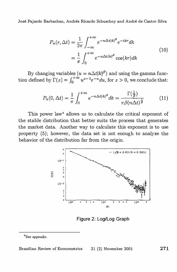
To calculate the characteristic exponent of stable distribution ((3), we estimated the probability of returning to origin P(r = 0) as function of 6.t (this approach was introduced by Mantegna (1995)). This value can be affected by the finiteness of data. Figure 2 shows P(r = 0) as function of 6.t, on a log-log scale, using different values for 6.t. We can adjust a straight line with a -0,63 inclination to these data. Up to the first 50 6.t values, the correlation coefficient of the adjustment is 0,985. As expected, we have a nonGaussian behavior. A test could be performed to check whether or not the difference is significant; however, since this is well-documented in literature, the test will not be carried out. The reason for the use of the probability of return to the origin as the basis for the calculation of characteristic "exponent {3 is that if we theoretically calculate this probability as function of 6.t, we obtain the power law, shown in Figure 2. In fact, if we take the definition of distribution:



Pn(r, b.t) = � 1+

= e-nL).tlkl" e-ikr dk 27r _=

.

= - e-nL).tlkl" cos(kr)dk 11+

= 7r 0

(10)

By changing variables (u = nb.tlkl,6) and using the gamma function defined by f(z) = It'" uz-1e-udu, for z > 0, we conclude that:

This power law· allows us to calculate the critical exponent of the stable distribution that better suits the process that generates the market data. Another way to calculate this exponent is to use property (5); however, the data set is not enough to analyze the behavior of the distribution far from the origin.

' r·----------------------------� , - l/� = 0.6:3 (R = 0.985)

, " .

,��--�� 100 :\ .! 5 101 :\ ·1 :, I()2 at

Figure 2: Log/Log Graph

4 See appendix.



3.1 Scale Invariance.

Some systems have something we call scale-free behavior; this means some kind of symmetry is preserved among the scales where systems are developed. This scale invariance occurs when some observation of the system presents a power law.

As the financial market is subject to accurate iteration rules, we verify there is room for scale invariance. Therefore, we will analyze some statistical properties of the stock market. We will see that the evolution of the financial assets returns or index is governed by a Levy-stable distribution.

After the characteristic exponent is known, we can observe that the different distributions are similar except for a scale factor, which means that, as previously mentioned, the stochastic process does not vary with time-scale transformations. To verify this property, it is possible to rescale all distributions to /';.t, submitting the variables to the following transformation:

e (12) r

Figure 3 shows that, except for large width events, the scaled distributions are superposed on a single distribution. This validates the thesis that financial markets, in general, have a self-similar timescale. This property gives us evidence that, in these markets, it is not possible to define a privileged time-scale in the system. A possible explanation could be the heterogeneity through which expectations and decisions are formed and the impact they have on price evolution. A set of negotiators that operate with different restrictions and time horizons produce a scale-free market dynamics. Perhaps the microstructure that sustains the existence of the market gives rise to a kind of amalgamation of relaxed times that follow the impact caused by new information.



'0'

10-1

10-�

-h.t=1 �h.t=5 --h.t= 10 --h.t = 20 � h.t = 30

1 0 -� 0;". 3;;---::0-0;0--0::-.-:-' -:co .:CO ---:0;'-. ':-----::0"::.2--0;:-.::-3 --::'0.'

' ..

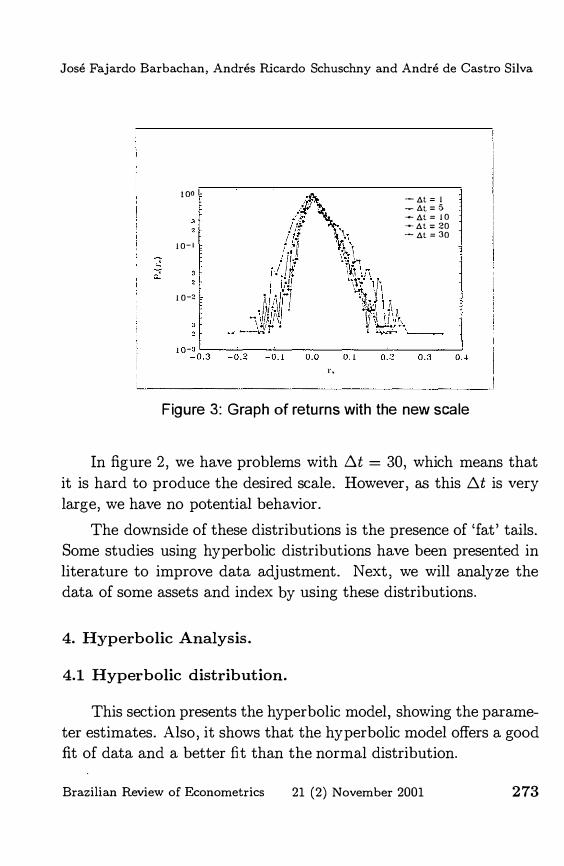
Figure 3: Graph of returns with the new scale

In figure 2, we have problems with /:;.t = 30, which means that it is hard to produce the desired scale. However, as this /:;.t is very large, we have no potential behavior.

The downside of these distributions is the presence of 'fat' tails. Some studies using hyperbolic distributions have been presented in literature to improve data adjustment. Next, we will analyze the data of some assets and index by using these distributions.

4. Hyperbolic Analysis.

4.1 Hyperbolic distribution.

This section presents the hyperbolic model, showing the parameter estimates. Also, it shows that the hyperbolic model offers a good fit of data and a better fit than the normal distribution.



The hyperbolic distribution function is built in such a way to present a linear histogram when constructed on a log-log scale. The curve with such behavior is the hyperbola, which is expressed as

y = -en,/! + X2 + {3x, (13)

with asymptotes of x -> +00 and x -> -00 respectively given by y = cpx and y = -"Ix where cp = 00+ {3 and "I = 00-(3. The domain of cp and "I is (0, 00) . The probability function correspondent to (13) is given by

a(oo, (3) exp ( -ooVl + x2 + (3x) , (14)

where a( a, (3) is a constant added to produce

1+00 -

00 a(oo, (3) exp ( -OOVl + x2 + (3x) dx = 1.

Now, take a = 4>�")' and (3 = 4>"2")', with this parametrization we can rewrite (14),

a(cp,'Y)exp (-� {CP[V(1 + x2) - xl + 'Y[v(1 + x2) + xl}), (15)

or, by multiplying the exponent III (15) by (VI + x2 + x)/( VI + x2 + x),

a(cp, "I) exp ( .:.-� {CP[V(1 + x2) + xl-1 + 'Y[V(1 + x2) + xl}) . (16)



To determine constant a( ¢, 'Y), we change the following variable: vex) = V(l + x2) + x, as v(-oo) = 0 and v(+oo) = +00, we have

+00

� J (1+v-2)exp (-�(¢v-l+'Yv)) dV= (17) o

+00 ( ) ( ) 1 1 x = - 1+ 1+ J 2 (V(1+x2) +x)2 V(1+x2)

-00

+00

= J exp (-%(¢v(X)-l +'Yv(x)) dx. -00

However the expression in (17) is equal to K-K1(K-)/w, where

1 K- = ffw and W = 1 1 ¢ +'Y (18)

and Kl is the modified Bessel function of the third kind and index 1 (see appendix). Thus, a(¢,'Y) = I<K�(I<)' where K- and ware given by (18). Therefore, once ¢ and 'Y are given, the probability distribution function is

f(x;¢,'Y) = K-K�(K-) exp (-�(¢ +'Y)(VI +x2) + �(¢-'Y)(x)) .

(19)



By including a location parameter f.L and a positive scale factor 8, we obtain, from (19),

w f(x;</>,'Y,f.L,8) = 8"K1(8,,) exp (-� (</> + 'Y)( J82 + (x - f.L)2) + � (</> - 'Y)(x - f.L)) .

(20)

Where we write ¢ and 'Y in the place of ¢ / 8 and 'Y /8,respectively. In equation (20), function In f(.; ¢, 'Y, f.L, 8) describes a hyperbola with slant asymptotes ¢ and 'Y. If we turn back to the initial parametrization, the hyperbolic probability distribution function will be given by

(21)

The hyperbolic distribution was proposed by Barndorff-Nielsen (1977). It was initially presented to model the movement of sand particles cast by winds with a continuous speed. That article suggests other applications for the hyperbolic distribution, such as financial data. Barndorff-Nielsen (1978) presents an application for the structure of income distribution. Eberlein and Keller (1995) were the first ones to use this distribution in finance.

The hyperbolic distribution is able to describe a considerable number of empirical distributions with asymmetric behavior or with 'fat' tails. Observe that this distribution has semi-heavy tails, that IS

276

hyp(x; 0<, (3, 8, f.L) ,....., e-(±a-;3)x when x -t ±oo

Brazilian Review of Econometrics 21 (2) November 2001


However, contrary to other distributions, the parameters of the hyperbolic distribution are apparently not able to provide much information on the distribution format. One way to study the form of distribution, suggested by Barndorff-Nielsen et al. (1985), is to write hyp(x; X,�, 8, j.L) using the following parameters

1

�= (1+8)a2-,62f2, and x=�,6/a. (22)

Such parametrization has the advantage of making � and X invariant even with scale and location transformations. The domain for parameter variation is given by

o ::; Ixi < � < 1. (23)

This domain is known as shape triangle and is represented in figure (4). The symbols N, N1, L, and E on the borders respectively indicate normal distribution, generalized inverse Gaussian distribution, with index). = 1, the Laplace distribution and the exponential.

-E � ___ L=--__ �--+ __ ----"L=--_� E

-w I

-1.0

1.0

0.0 N

W I

Figure 4: Variation domain of paramaters

Brazilian Review of Econometrics 21 (2) November 2001

1.0 X

277


All these distributions are limits to the hyperbolic distribution. This allows us to understand � and X asymptotically as kurtosis and asymmetry.

To obtain the distribution limits, Barndorff-Nielsen et aL (1985) chose 8 so that the variance of the hyperbolic distribution could be equal to 1 and the mean could equal 0. With these simplifications, the distribution assumes the following shape

hyp(x; �,X) = a(�,x)exp (-b(�,x) [Jl- (X/�)2 + z2 - (xm2z] ) ,

(24) where x X

z = �-l -1 + Z'

a(�, X) = [2(Cl - 1)KdC2 - IW1 , and �-2 -1

b(�,X) = 1 - X/(

With � --t 0, we have the normal distribution

_1 exp ( _ _ 1 ) . y"iif 2x2

With � --t 1, we have the Laplace distribution

exp (- 2 2

(Ixl- XX)) . I-X

For X = 0, in particular, we have e-2Ixl. For Ixl--t 1, we obtain the exponential distribution. The generalized inverse Gaussian distribution is obtained by X --t ±�. The moment-generating function of the hyperbolic distribution is given by



Eberlein et al.(1998) obtain this expression by using (21) with Vo.2_j32

J-l = O. Therefore, we have a(a, f3, 0) = ( �).

Forff3 + tf < a

M(t) = J etx f(x; a, f3, 0, O)dx

2o.6K1 6y o.2_j32

= a(a, f3, 0) J exp( -av02 + x2 + (f3 + t)x)dx

a( a, f3, 0) a(a, f3 + t, 0)

Va2_f32 K1ova2-(f3+t)2 Kl(ova2-f32) va2-(f3+t)2

(2 6)

(2 7)

(2 8)

Thus, all the moments of the function exist. For the expected value and for variance, we obtain,

(2 9)

(30)

where X � hyp (x; a, f3, 0, J-l) and ( = oa2 - f32 In the following section, we will see how we can use this distribution to model the returns.



4.2 Return model.

In this context, let us suppose that the price of assets are modeled by the following equation

Where {Xdt;:o:o is a Levy process generated by the hyperbolic distribution. Now we can define returns Rt as

St � St Rt = log -- � -- - 1, St-l St-l

We observe that the right-hand side approximation occurs when the difference between today's and yesterday's closing price is small. Observe that if we actually define

we would have

As most authors do, we will use the one that corresponds to a continuous composition. The main reason is that the return in n periods would be given by:

(St+n) Rt+1 + ... + Rt+n = log ---s; , this is not satisfied by 11;. In addition, we should not forget that

for continuous time processes, the continuously compound rate of



return is a natural choice. If the prices were lognormal, that is, if

Xt were a normal variable or more specifically a standard Brownian

motion, we would have

Rt = Xt - Xt-1 � N(O.l) Therefore, lognormality of prices would imply normality of re

turns, so we need another model for prices or for returns. Our can

didate to be tested will be the hyperbolic Levy motion, that is, the Levy process generated by the hyperbolic distribution. For that reason, we have to estimate the parameters of this distribution by using the real data of Brazilian Market to check whether the candidate is a good substitute for the geometric Brownian motion which, as already mentioned, has several flaws. Next, we will present this estimation.

4.3 Parameter estimates.

We estimate the hyperbolic distribution parameters using the Hyp program developed by Blresid and S0rensen. The estimation is made by maximum likelihood with the hypothesis of the independent and identically distributed random variables. See Blresid and S0rensen (1992) for the description of the algorithm. The results are

shown in Table 1.

Based on the construction of the hyperbolic distribution, it is necessary to have a great number of data in the sample so that we

can obtain a reasonable estimate of tail behavior. We should expect

this restriction not to influence the use of the hyperbolic model in

finance due to samples with a large number of data.



Table 1: Estimation of hyperbolic distribution parameters.

(i 7J '8 ji Ibovespa (G 1) 49.53 -3.939 1.638E-09 3.689E-03 Ibovespa (G2) 66.59 -7.430 5.937E-09 5.092E-03 Telebras (Gl) 43.67 -2.704 8.488E-03 4.012E-03 Telebras (G2) 56.37 -4.136 7.291E-03 4.920E-03 Petrobras (Gl) 42.58 -1.804 9.359E-03 2. 578E-03 Petrobras (G2) 54.95 -3.437 7.488E-03 4.952E-03

Like Eberlein and Keller (1995), we used the X2 test to analyze

the adherence of data to the hyperbolic distribution. The estimated

:\:2 values and the critical value of variable X� with a significance

of 1% are shown in Table 2. The degrees of freedom are given by

l! = k - 1 - m, where k is the number of classes and m = 4 is the

number of estimated parameters. In all cases, we have :\:2 < X�=l%' which does not let us reject the null hypothesis of the hyperbolic behavior.

Table 2: X2 with hyperbolic distribution for Ho

Ibovespa (G 1 ) 17.250 21.666 Ibovespa (G2) 9.283 18.475 Telebnis (Gl) 12.070 20.090

Telebras (G2) 9.687 20.090 Petrobras (Gl) 13.601 18.475 Petrobras (G2) 16.937 18.475

It is important to emphasize that if we change the significance level to 5%, we will reject the null hypothesis in 2 cases, which would not let us obtain more robust results.



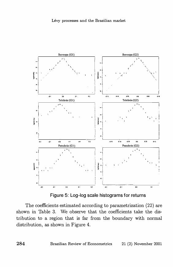
Figure 5 shows the histograms of data and their estimated density. The graphs are represented on a logarithmic scale so that the adjustment can be viewed more easily. If the returns follow the hyperbolic distribution, their log histogram should present an increasing and then a decreasing line. The simplest curve with such behavior is the hyperbola. We note that the theoretical curves are in

agreement with the observations, especially regarding the data that are closer to the mean. However, for tail data, there are off-curve points. This could make us think that the use of these distributions

would be inappropriate. If we find the Kolmogorov distance (KD)

and Anderson-Darling statistic (AD)' we can observe that the adjustment obtained through the hyperbolic distribution is far better than that made via normal distribution, as shown in the following

table.

DK(hyp) DK(normal)AD(hyp) AD (normal)

Ibovespa (Gl) 0.0243382 0.0892196 0.649622 4518.23 Ibovespa (G 2) 0.032024 0.10132 0.69617 2043.33 Telebnis (Gl) 0.020799 0.075921 3.3639 96156.3 Telebnis (G2) 0.015393 0.076458 0.355854 782.979 Petrobras (Gl) 0.015592 0.071611 3.3639 96156.3 Petro bras (G2) 0.033111 0.067329 0.355854 4550.97

This can also be seen in Figure 5, since the graph of lognormal density would be a parabola, which would leave more points off the

curve. In case of the stable Paretian distribution, we would have a straight line, which would also be an extreme case.

SSee appendix.


.J

f " � ,

. i ,1

I

oj,

I LJ ' I I

,j .,

, :1 H , , I '! ,1 ,


Ibovc:spa (GI)

'.

"

" ; ,

"

Tekbras(Gl)

,�,

, '

.. "

Petrobras (G 1) , '""'.,

"

oj oj

� I I i '"1 1� I

.j

"j <>� '" i I "I

.' ,

I 'I'� I

I "1 oi '" i i .,.J , I ,4

• i

"

."

. " ."

Jbovespa (G2)

' '

-'

.. ..

Telebr.is (02)

, -<--,

.. ..

Petrobnis (G2)

L�� ______ . , ..

Figure 5: Log-log scale histograms for returns

'-,'-

"- , '\

.. " .

."

-----, , !

"

The coefficients estimated according to parametrization (22) are shown in Table 3. We observe that the coefficients take the dis

tribution to a region that is far from the boundary with normal

distribution, as shown in Figure 4.



Table 3: Shape triangle parameters.

� X Ibovespa (G 1) 1.0000 -0.0795

Ibovespa (G2) 1.0000 -0.1116 Telebras (G 1) 0.8544 -0.0529

Telebras (G2) 0.8422 -0.0618 Petrobras (Gl) 0.8457 -0.0358

Petrobras (G2) 0.8420 -0.0527

4.4 Scale Invariance.

To analyze the scale invariance, we have to use a result obtained

by Barndorff-Nielsen and Prause (200l) , which shows that distributions with semi-heavy tails have an apparent invariance; therefore, as

previously observed, hyperbolic distributions have semi-heavy tails and, consequently, do not have scale invariance.

5. Conclusions.

Based on the previous analysis, we may conclude that the adjustment obtained through the hyperbolic distribution is good and

as a consequence better than the adjustment made via normal distribution and via the stable Paretian distribution, as the former has

a very light tail and the latter, a very 'fat' tail. Hyperbolic distributions have semi-heavy tails, which allow better adjustment for

some series at a given significance level. In addition, we noted that

the parameters do not have a clear meaning; however, by changing parameters, it is possible to understand � and X asymptotically as kurtosis and asymmetry, respectively.

Hopefully, we expect to have achieved our goal by showing some

empirical evidence and discussing the use of continuous time distributions for the analysis of the Brazilian market.



6. Appendix.

6.1 Power Law.

We say that N has a potential behavior and follows a power law when

N(s) ex: so.

6.2 Bessel Functions.

The modified Bessel function (K>-l has the following integral representation

x > 0,

Some basic properties:

L

2.

6.3 Generation of Levy Processes.

Take {Xth;::o as the Levy process generated by the hyperbolic distribution with hyp density, i.e., the process with independent and

stationary increments such that Xo = 0 and the distribution of Xl



has hyp density. When J.L = 0, Eberlein and Keller (1995) called {Xt}t::o:o Hyperbolic Levy motion.

The mean and variance are finite, and this was previously calcu

lated; however, we can observe that E IXtlP < 00, '<It;:::: 0, (p;:::: 1).

6.4 KD and AD.

Take {Xth::o:o as the Levy process generated by

Let us suppose that F(x) is an accumulated distribution func

tion, therefore, Kolmogorov distance is given by

DK = maxlFempirical(X) - Festimated(X)I , xElR.

and Anderson-Darling statistic is given by:

AD _7=IF� e�m� p�i�ri�c a�I'f. (=; X,,=) ;=-=F.�ei'ist�i m= at� e:; d",( x=)�I=:=i' = max xElR. VFestimated(X) (1 - Festimated(X))

Submitted in December 1999. Revised in March 2002.

References

Abramowitz, M. & LA. Stegun 1968. Handbook of Mathematical

F unctions . Dover, New York.

Barndorff-Nielsen, O.E. 1977. "Exponentially decreasing distributions for the logarithm of particle size". P roceedings of the Royal

Society London, A 353:401-419.

Barndorff-Nielsen, O.E. 1978. "Hyperbolic distributions and distributions on hyperbolae". Scandinavian Journal of Statis t ics,

5:151-157.



Barndorff-Nielsen, O.E. 1997. "Processes of Normal Inverse Gaus

sian Type". Working Paper Series no. 1, Center for Analytical Science, Aarhus School of Business.

Barndorff-Nielsen, O.E., P. Blaosid, J.L. Jensen, & M. K Sprensen

1985. "The fascination of sand", in Atkinson, A.C. Fienberg,

S.E. (eds.), A celebration of statistics, 57-87, Springer: New

York.

Barndorff-Nielsen, O.E. & K Prause 2001. "Apparent Scaling". Finance and Stochas tics, 5:103-113.

Blaosid, P. & M. K Sprensen 1992. "Hyp- a computer program for analyzing data by means of the hyperbolic distribution" , Re

search Report no. 248, Department of Theoretical Statistics, University of Aarhus.

Duarte J., A.M. & B.Y.M. Mendez 1999. "Robust Estimation for ARCH Models". Brazilian Review of Econometrics, 19:139-180.

Eberlein, E. & U. Keller 1995. "Hyperbolic distributions in finance", Bernoulli, 1:281-299.

Eberlein, E., U. Keller & K Prause 1998. "New insights into smile, mispricing and value at risk: the hyperbolic model", Working Paper n. 39 (revised version), Center for Data Analysis and Model Building, University of Freiburg.

Fama, E. 1965. "The behaviour of stock market prices" , The Journal

of Busines s, 38:134-105.

Issler, J.V. 1999. "Estimating and Forecasting the Volatility of Brazilian Finance Series Using ARCH Models". Brazilian Re

view of Econometrics, 19:15-56.

Kuchler, U., K Neumann, M. Sprensen & A. Streller 1994. " Stock returns and Hyperbolic distributions", Discussion paper 23, Sonderforschungsbereich 373, Humboldt-Universitiit zu Berlin.



Levy, P. 1937. "TMorie de l'Addition des Variables Aleatories, Gauthier-Villars, Paris.

Mandelbrot, B. 1963. "The variation of certain speculative price" ,

The Journal of Business, 36:4394-419.

Mandelbrot, B. 1997. "Fractals and Scaling in Finance". Springer

Verlag.

Mandelbrot, B. & H. Taylor 1967. " On the distributions of stock

price differences". Operations Research 15:1057-1062.

Mantegna, R. 1995. "Scaling Behaviour in the Dynamics of an

Economic Index". Nature, 376:6535,46-49

Mazuchelli, J. & H. S. Migon 1999. "Modelos GARCH Bayesianos: Metodos Aproximados e Aplica<;6es". Braz ilian Review of

Econometrics, 19:1, 111-138.

Pereira, P.L.V., L.K. Hotta, L.A.R. Souza & N.M.C.G. Almeida, 1999. "Alternative Models to Extract Asset Volatility: A Comparative Study". Brazilian Review of Econometrics, 19:1, 57-109.


Levy processes and the Brazilian market Jose …Levy processes and the Brazilian market Jose Fajardo...

Documents

Transcript of Levy processes and the Brazilian market Jose …Levy processes and the Brazilian market Jose Fajardo...