Let them Have Choice:

Gains from Shifting away from Employer-Sponsored

Health Insurance and Toward an Individual Exchange

Leemore Dafny1, Kate Ho and Mauricio Varela

July 2011

Abstract

Most nonelderly Americans purchase health insurance through their employers, which sponsor a limited number of plans. Using a panel dataset representing over 10 million insured lives, we estimate employees’ preferences for different healthplans and use the estimates to predict their choices if more plans were made available to them on the same terms, i.e. with equivalent subsidies and at large-group prices. Using conservative assumptions, we estimate a median welfare gain of 13% of premiums. A proper accounting of the costs and benefits of a transition from employer-sponsored to individually-purchased insurance should include this nontrivial gain.

1 Kellogg School of Management, Northwestern University and NBER. Email: l-dafny@kellogg.northwestern.edu. Columbia University, Economics Department and NBER. Email: kh2214@columbia.edu. Kellogg School of Management, Northwestern University. Email: m-varela@kellogg.northwestern.edu We are grateful for helpful comments by seminar participants at Boston University School of Management, University of Chicago (Harris), RAND, Yale Economics Department, Yale School of Public Health, and the American Economic Association Annual Meeting.

1

1. Introduction

Nearly 60 percent of nonelderly Americans purchase employer-sponsored health

insurance (ESI).1 Although there are no legal impediments to offering a broad array of plans, in

practice employers offer a very limited set of choices: a 2005 survey by the Kaiser Family

Foundation/Health Retirement Education Trust finds 80 percent of employers who offer

insurance provide only one option. The restriction of employee choice may prevent individuals

and families from selecting the healthplan that best suits their needs, and from trading off added

benefits against the associated premium increases.

As the U.S embarks on the most aggressive healthcare reform since the introduction of

Medicare in 1965, the possibility of leveling the playing field between group and individual

insurance (through a variety of means) has come to the fore. Many have expressed concerns

about the erosion of employment-based coverage, but researchers have not systematically

examined, let alone quantified, the benefits associated with individual choice of insurance. In

this paper, we use a large panel dataset on employer offerings and employee choices to infer the

gains consumers would enjoy were they able to select from a broader spectrum of plans in their

local market, holding constant employers’ spending on employee subsidies and the full tax-

deductibility of premiums. By quantifying the gain to individuals from being able to select any

plan available in their local market, we back out the amount by which prices would have to

increase to fully offset this gain. In so doing, we provide policymakers with guidance regarding

the implementation and design of reforms that bolster individual choice. In a companion paper

(Dafny, Ho and Varela 2010), we examine the distributional consequences of expanded choice 1 Using data from the March 2010 Current Population Survey, Fronstin (2010) reports 59 percent of the non-elderly population had employment-based health benefits in 2009. The analogous figure for 2000 is 68.4 percent (Fronstin 2008).

2

and contrast the characteristics of plans selected by employers and those that would be selected

by employees if they were available on the same terms.

We use a unique dataset of employer plan offerings and employee plan selections for a

national sample of 800+ large U.S. employers during the period 1998-2006, representing over 10

million insured lives in every year. Our approach consists of three distinct components. First,

we estimate a discrete choice model of employee demand for healthplans, conditioning on the set

of plans offered by the relevant employer in the relevant geographic market and year. The

parameters from this model reflect the values placed by employees on individual plan

characteristics. Second, we estimate a hedonic model of premiums that permits us to predict the

premiums a given employee would face for each plan offered in her local market. Third, we use

the demand estimates, together with the predicted premiums, to predict employee choices of

plans and their expected utility when offered additional plans currently existent in that market

and year. The counterfactuals are budget-neutral for employers; that is, their total contributions

to health insurance are held constant. Conceptually, the counterfactual is akin to granting

employees a voucher equal to their employer’s present contribution to health insurance, valid for

the purchase of insurance plans on the individual market (which could be a regulated

“exchange”). We use the results to estimate the amount by which premiums would need to

increase (relative to the levels predicted by our hedonic model, which implicitly assumes group-

based pricing due to the underlying data) to fully offset the net gain in consumer surplus.

We find choice is worth quite a bit for most individuals: in our most conservative

hypothetical scenario the median employee would enjoy a surplus gain of roughly 13% of

combined employer and employee premium contributions. In year 2000 dollars, this gain is

approximately $310 per individual or $1,240 for a family of four. Combining these figures with

3

data on employer subsidies, we find the median employee would be willing to forego 16 percent

of her employer subsidy simply for the right to use what remains toward a plan of her choosing.2

(As an analogy, consider the employer who offers her employee a choice of heavily subsidized

vehicles: the Ford Focus or the Cadillac Escalade. The employee would trade a non-trivial

percent of the employer subsidy in exchange for the freedom to use the subsidy toward her most-

preferred vehicle, assuming it is available at the same price as currently paid by employers who

buy in bulk.) Of course, we do not anticipate the net benefits of choice to be as large as our

estimates, since premiums are likely to increase with the devolution of insurance to the

individual marketplace, and there are costs associated with the proliferation of choice. However,

a complete accounting of an exchange proposal should include some estimate of the value of

choice.

We caution that our results provide a conservative estimate of this value (or, equivalently,

a low estimate of the premium increases that would offset the benefits of choice). First, our data

enable us to build a very rich logit model of choice for a given set of employees, but we do not

incorporate differences in preferences across individuals within employee groups except through

a random error term. There may be substantial gains from better matching of individuals to

plans. Second, due to the well-known limitations of the logit choice model, we do not expand

the choice set to include all plans we observe in a given market, except to provide an upper-

bound estimate of the value of choice. In fact the conservative scenario mentioned above holds

constant the number of plans in the choice set and simply switches the observed options with

those that are most preferred by employees in the relevant firm and market.

2 This estimate is obtained from our preferred specification, described below; estimates from other models are also presented.

4

The paper proceeds in seven sections. Section 2 discusses the recent trends in the degree

of choice in employer-sponsored plans and summarizes related research. Section 3 describes the

data. Section 4 presents the estimation strategy and results for the demand and hedonic models

used as inputs into the simulations presented in Section 5. Section 6 discusses the implications

of the results, and Section 7 concludes.

2. Background

2a. Employer-Sponsored Insurance Plans: How Much Choice Is There and How is This

Changing?

Most workers who receive insurance through their employers have a choice of plans but

this choice can be quite limited. The Kaiser Family Foundation/ Health Research and

Educational Trust Employer Health Benefits Annual Survey (hereafter Kaiser/HRET survey)

studies the percentage of workers with job-based coverage, the kinds of plans employees offer

and the choices made. Approximately 2,000 randomly selected employers are surveyed, covering

a range of industries and both public and private firms. The survey indicates that sixty percent of

firms, and ninety-eight percent of firms with over 200 workers, offered health benefits in 2005.

As mentioned earlier, eighty percent of firms sponsoring insurance offered a single plan.

However, Figure 1 shows that larger firms offered more choice than smaller firms: twenty-seven

percent of large firms (those with 1000-4999 workers) and only seventeen percent of firms with

over 5,000 workers offered a single plan. Overall, sixty-three percent of covered workers could

choose from multiple healthplans.

The most common healthplan offered to workers in 2005 was a PPO plan: 82% of

covered workers had access to this type of plan. Figure 2 documents that 28% of covered

5

workers had access to a POS plan, 44% had access to an HMO and only 12% had access to a

conventional indemnity plan. Indemnity plans have become less widely available over time

while the availability of PPO plans has increased dramatically since 1988. The patterns in the

dataset we use are similar to those in the survey, although our sample is skewed towards larger

firms so that choice is less limited than is the case for the average employee. For example, in

2005, about half of the employee groups in our sample are offered a single option. The choice

sets observed in our data are discussed further in Section 3.

2b. How Do Employees and Employers Choose Among Plans?

Several studies in the health economics and health policy literatures investigate the

factors influencing employees’ choice of healthplans. A much smaller set of papers examine

employer decision-making, with an emphasis on whether healthplan quality affects employer

choices. To our knowledge, no study combines empirical analysis of both decisions, preventing

any quantitative assessment of the tradeoffs associated with allocating decision rights to one or

the other party. In the review that follows, we focus exclusively on studies that pertain to the

working population, as our data includes only active employees.

2b.i. Employee Choice of Healthplans

Most studies in this category focus on the sensitivity of employees to variations in plan

price and quality, as measured by items included in the Health Plans Employer Data and

Information Set (HEDIS) and the Consumer Assessment of Healthcare Providers and Systems

(CAHPS) survey.3 Elasticities are reported for various definitions of price (or premium):

with/without employer contributions; pre or post-tax. Here we discuss estimates of the elasticity

3This survey primarily addresses consumer satisfaction, and is maintained by the governmental Agency for Healthcare Research and Quality (AHRQ).

6

of within-employer-group enrollment with respect to pre-tax employee contributions, which

corresponds to our model below.

Two studies identify these elasticities using the plan choices of university employees

following implementation of a fixed-contribution arrangement, under which employees bear the

incremental cost of their plan choices. Royalty and Solomon (1999) report estimates between

-0.28 and -0.62 for Stanford employees; this compares closely with Cutler and Reber’s (1998)

estimates for Harvard employees (-.30 to -.60).4 Two recent studies give more divergent

estimates. Using data on plan choices of employees in eleven small and mid-size firms in the

Western U.S. during 2004-2005, Levin, Bundorf, and Neale (2010) find elasticities in the upper

tail of the range cited above (approximately -0.57, per our calculations from reported semi-

elasticities). In contrast, Carlin and Town report an elasticity of demand around -0.06, using an

autoregressive, multinomial probit choice model estimated on data from a large, self-insured

employer between 2002-2005. Levin et al. observe this lower estimate may be due to the well-

known fact that elasticities are higher for initial plan choice (the key decision in the Levin et al.

paper), whereas Carlin and Town identify the response to price through plan switchers.

Significantly, Carlin and Town report somewhat higher elasticities from multinomial logit

specifications, the model most commonly utilized in this literature. Our own estimates (from a

multinomial logit model) vary by industry and other employee characteristics; across the entire

sample, however, our estimate is -0.28. As with Carlin and Town, identification relies in part

(although not exclusively) on plan switchers.

The relevant studies that consider the sensitivity of employee decisions to healthplan quality

include Wedig and Tai-Seale on federal employees (2002), Beaulieu on Harvard employees

4 Royalty and Solomon also report much higher estimates (exceeding -1) for models with individual fixed effects, however in this case identification stems from post-implementation price changes, the sources of which are unclear. The authors refer to -0.55 as their average estimate from “preferred” specifications.

7

(2002), and Scanlon et al (2002) and Chernew et al (2008) on General Motors employees.

Generally speaking, these studies find modest reactions to quality information. It is possible

these aggregate effects mask larger responses by populations with stronger incentives to respond,

however, the evidence to date on this matter is mixed.5

2b.ii. Employer Choice of Healthplans

Research on how employers make decisions regarding which plans to offer, and how

many, is limited by comparison. We focus here on empirical analyses of plan offerings, as

opposed to analyses of surveys that ask employers to report what factors affect their decisions

(e.g. Rosenthal et al. 2007). The most relevant papers for our purposes include Bundorf (2002)

and Chernew et al (2004). These papers focus on whether employers’ decisions reflect the

assumed needs of their employees. For example, Chernew et al (2004) uses data on the HMO

plans offered by 17 large employers in 2000 to see whether CAHPS scores affect the propensity

any given plan is offered; they find that employers are more likely to offer plans with strong

absolute and relative CAHPS performance measures. In related work, Bundorf (2002) finds

employers’ offerings correlate with employee characteristics. For example, firms whose

employees have greater variation in healthcare expenditures are more likely to offer a choice of

plans.

Our project builds on this research by quantifying – in dollars - the loss to consumers

associated with restricted choice, and comparing these estimated losses to premium increases

5 Scanlon et al. (2002) find new hires and plan switchers are more responsive to quality measures as well as price. Using the same study population, Chernew et al (2008) report “no significant evidence of heterogeneity” in the valuation of plan attributes based on observable or unobservable employee characteristics. Evidence from a different population – namely Medicare enrollees – is mixed as well. Using enrollment data surrounding the release of Medicare HMO report cards in 2000 and 2001, Dafny and Dranove (2008) find no differences in responses by demographic characteristics at the county level, but stronger evidence of non-report-card-related learning about quality (“market-based learning”) in counties with greater HMO penetration, more private report card data, and more stable populations.

8

likely to occur if employees are free to apply their employer subsidies to other plans offered in

their marketplace.

3. Data

We use a proprietary panel database on healthplans offered by a sample of large, multi-

site employers from 1998-2006. The dataset, which we call the “Large Employer Health

Insurance Dataset” (LEHID), was provided by a major benefits consulting firm which assists

employers with designing or purchasing benefits from health insurers.6 The unit of observation

is the plan-year. A plan is defined as a unique combination of an employer, geographic market,

insurance carrier and plan “type” (HMO, POS, PPO and indemnity), e.g. Company X’s

Chicago-area Aetna HMO. The full dataset contains information from 813 employers and 139

geographic markets in the United States. The markets are defined by the data source and

typically delineate metropolitan areas and ex-metropolitan areas within the same state, e.g.

Arkansas – Little Rock and Arkansas – except Little Rock.7 The number of enrollees covered in

the data averages 4.7 million per year. Given an average family size above 2, this implies more

than 10 million Americans are represented in the sample in a typical year. After excluding

observations with missing or problematic data8, the sample contains 811 employers, 139 markets

and 356 carriers. Most employers are active in a large number of markets (45 for the median

employer-year). Descriptive statistics are set out in Table 1. For additional details of the data,

see Dafny (2010).

6 Using a survey of 21,545 private employers, Marquis and Long (2000) find that external consultants were employed by nearly half of the smallest firms (<25 workers) and nearly two-thirds of the largest firms (>500 workers). This suggests that the results of our study will be generalizable beyond our specific sample. 7 Dafny (2009) includes a map of the geographic markets, which occasionally span state lines. 8 We drop 347 observations with a missing industry code, 2752 observations associated with employer-market-years in which the employee share of premiums for one or more plans is negative, and 304 observations with missing data. We also consolidate the four plans that appear twice in the data because the employer self-insures some enrollees and fully-insures others.

9

Premium is the average annual charge, normalized to year 2000 dollars using the CPI, per

person-equivalent covered by a plan.9 It combines employer and employee contributions. The

definition of premium depends on whether a plan is self-insured or fully insured. Many large

employers choose to self-insure, outsourcing benefits management and claims administration but

paying realized costs of care. Such employers can spread risk across large pools of enrollees,

and often purchase stop-loss insurance to limit their exposure. Per ERISA (the Employee

Retirement Act of 1974), these plans are also exempt from state regulations and state insurance

premium taxes, enabling firms to reduce their insurance costs and/or standardize plan benefits

across multiple sites. Reported self-insured plan “premiums” are actually estimates of

employers’ projected healthcare expenditures, including any administrative fees and stop-loss

premiums.10

Demographic factor is a measure that captures the family size, age, and gender of

enrollees in a given plan-year. It can be construed as the mean number of “person equivalents”

per enrollee. Plan design captures the generosity of benefits for a particular plan-year, including

the level of copayments required of enrollees. Both factors are calculated by the source, and the

formulae were not disclosed to us.

Our empirical analyses use the employer-market-year as the unit of observation. If an

employer appears in the sample in a given year, all healthplans it offers in any market are

included in the data. However, the panel is unbalanced: on average, 240 employers appear in the

sample each year. Of the unique employer-market pairs in the data, 46 percent appear only

once, and 17 percent appear twice. We do not observe the total number of employees offered

9The original data reports the average premium per enrollee. Thus, this average premium is larger for employee groups whose enrollees cover more dependents. We follow the practice of our data source and divide this figure by demographic factor to obtain the premium “per effective enrollee.” 10 This definition of premiums for self-insured plans is common to all employer surveys, including the KFF/HRET survey described in Section 2.

10

insurance, hence our analyses are limited to employees who do take up coverage. As additional

employees may take up coverage if more options are available, this likely understates the total

gains from expanding choice.11

Before moving to the empirical analysis, we present statistics on the state and evolution

of choice within our sample and study period (Figure 3). As expected, choice is more common

among employers in our sample than among the universe of employers sampled by the

Kaiser/HRET survey, however nearly half of the employer-market-years offer access to only one

plan. Over 75% offer at most two plans. Fifty percent of those offering two plans offer an HMO

and a PPO; 14% offer a POS plan and a PPO. The figure also shows that the amount of choice

offered has fallen over time and (consistent with the survey evidence) that PPO plans have

increased in popularity while indemnity plans have become less popular.

4. Empirical strategy

We conduct our analysis in three steps. First we use our data on consumer choices of

health plans conditional on the options offered by their employers to estimate a utility equation

describing employee preferences for plan characteristics. Second, we estimate a hedonic

equation that describes the relationship between the premiums we observe in the data and plan,

employer and market characteristics. We use the coefficient estimates from this equation to

predict the combined employer and employee premiums that employees in a given firm, market

11 To estimate the share of employees who do not take up employer-sponsored insurance, we matched our data to total employment figures reported in the Compustat Financial Database. However,Compustat is limited to large, publicly-traded firms, substantially reducing our sample size. In addition, the employment figures are very noisy, particularly as some firms report employment for North America rather than for the United States. The implied mean enrollment rate across employer-years was 46%, much lower than the 67% reported by the Kaiser-HRET survey for large firms (200+ workers) offering health benefits in 2005. We concluded that the analyses using this matched data sample are less informative than those utilizing the entire sample, notwithstanding the loss of an “outside option” in our choice model.

11

and year would face for every plan offered in their market and year, assuming large-group

pricing prevails. Last, we use the results of both analyses to predict employee choices and

expected utility under our counterfactual scenarios in which additional plans are made available

on the same terms (i.e. a fixed percentage subsidy for a given set of employees, group rates and

full tax-deductibility).

Although we are interested in the effect of expanding consumers’ choice sets to encompass

all possible options, the structure of our utility equation (which includes a logit error term with

unbounded support) implies that adding all available plans to the choice set would over-estimate

the welfare gains of choice. We therefore investigate three counterfactual scenarios. First, we

maintain the same number of plans in the choice set for each employer-market-year, but we

substitute the most preferred plans for those currently offered (that is, if the employer does not

choose optimally for its employees). We call this the “plan swapping” scenario. Second, we

assume that employees within each employer-market-year triple gain access to their preferred

option within each of three plan types: HMO, POS and PPO plans.12 (We exclude indemnity

plans because they are rarely offered in our data. Employers already offering indemnity plans

receive their most-preferred indemnity plan in the counterfactual to ensure a strictly expanded

choice set.) We call this the “all plan types” scenario. Third, we make all plans in the market-

year available to all employees (the “all plans” scenario). The changes in consumer surplus

predicted by the “plan swapping” and “all plans” scenarios provide lower and upper bound

estimates, respectively, of the value of greater choice, with the “all plan types” scenario falling in

between.

12 If an employer previously offered more than one option within a given plan type, we retain the same number of options within that plan type in the simulation.

12

4.a. Demand Model

The first step is to estimate a model of consumer demand for healthplans. We use a logit

model, including in the consumer’s choice set only the plans that are offered by the relevant

employer in the relevant market and year. We denote a “plan” as a unique employer-market-

carrier-plantype-year quintuple, the unit of observation for our data. Consumer i’s utility from

plan emcjt in year t is modeled as:

u (1) imcjt imcjtemcjt

where emcjtemcjtemtemtemcjtemcjt px : a linear combination of observed characteristics of the

plan (denoted x), premium (p), and an unobserved quality variable )( . The coefficients on plan

characteristics and premium are permitted to vary across employee groups (described in detail

below). The term imcjt is consumer i’s idiosyncratic preference for carrier c and plantype j in

market m at time t.

Before discussing the details of our estimation, we offer remarks on our use of a simple

logit model rather than a nested logit or random coefficients model. The most intuitive nested

logit model, in which the first nest is the choice of plan type (such as HMO or non-HMO) and

the second is the choice of plans within type, requires eliminating most of the data because

choice sets typically contain at most one of each plan type. A random coefficients model, though

feasible, is unnecessary as our data afford us the opportunity to explicitly model heterogeneity in

preferences through a large set of fixed effects and interactions between plan characteristics and

observable characteristics of the relevant employee population. These terms, which we discuss in

detail below, permit the coefficients on the key explanatory variables to differ across observably

different groups of consumers.

13

Berry (1994) shows that the parameters in equation (1) can be estimated using the

following linear equation, which explicitly lists all covariates:

emcjtemcjt

iemcjtiemcjt

emcjjtmcejtii

emcjtiemcjtemcjtemcjt

eijti

mjmtmcemtjcmetem

redπself-insu

signi)*plan deI(industryμgnψplan desi

*prphic factoi)*demograΙ(industryαΣ

piindustryfactorcdemographipp

iindustrys

*)( *

)( )ln()ln(s (2)

4

321

0emcjt ηψ

In equation (2), emcjts is the market share of plan emcjt and em0ts is the market share of the

outside option in the relevant employer-market-year triple. We define the “outside option” to be

the most frequently-offered plan in the employer-market-year triple, which implies normalizing

its unobserved quality to zero. Other plans’ observed characteristics are measured relative to

those of this baseline plan.13 For robustness, we also report results obtained when the outside

option is the least generous plan in the relevant employer-market-year triple. 14

The covariates include several fixed effects, two continuous measures - plan design and

the employee’s contribution to premiums (“price”) - and interactions including these two

measures. We discuss each in turn.

The fixed effects include all of the “main effects,” that is, dummies for each employer,

market, carrier, plan type, and year. However, the dummies for employer, market and year are

differenced out when we normalize the characteristics of each plan with respect to those of the

baseline plan, which implies we obtain coefficient estimates only on carrier and plan type

13 In the case of a tie the most frequently-offered plan is designated as the plan with the largest number of enrollees in the market-year. 14 The least generous plan is defined using plan type and premium. Indemnity plans are the most generous, followed by PPOs, POS plans and HMOs in that order. Within a particular plan type, the cheaper of a pair of plans is defined as the less generous plan.

14

dummies. Carriers and plan types with the largest coefficient estimates generate higher utility,

ceteris paribus, for enrollees.

It is also possible to include second, third, and fourth-order fixed effects. Such terms

have the advantage of enabling a better fit of the model, but there are four important

disadvantages. First, they absorb variation in continuous regressors of interest such as price,

leaving little to identify the coefficients on these measures. Second, many of these terms cannot

be included in the counterfactual scenarios. For example, employer-carrier fixed effects would

capture the mean utility of different carriers to employees of a particular firm. In a

counterfactual that expands the choice set to include carriers not presently offered by that firm, it

would not be possible to estimate the utility of the new options. Third, even if a coefficient

could technically be estimated for a third or fourth-order interaction term, the number of

observations identifying it would be small and therefore unlikely to yield a representative

estimate valid for counterfactual simulations. Last, some of these terms raise endogeneity

concerns. For example, employer-year interactions would capture the fixed utility associated

with the set of plans offered by an employer in a given year, but this depends on choices

currently on offer, and would presumably change when the choice set changes.

In recognition of these issues, we include a parsimonious set of second-order interaction

terms that control for the most important unobservable correlates of utility while permitting

estimation of our counterfactual scenarios.15 Two of five interactions we include will be

“differenced out” in our specifications: employer-market fixed effects and market-year fixed

effects. We mention them here to clarify the sources of identification for coefficients in the

15 Of the 10 possible second-order interaction terms, we include five for reasons detailed in the text that follows. We exclude employer-year interactions due to endogeneity concerns, and employer-carrier and employer-plan type interactions because these are not compatible with our counterfactual simulations. Finally, carrier-plantype and carrier-year interactions are unlikely to be important determinants of unobserved quality. Indeed, we find our price elasticities are unaffected by excluding these terms.

15

demand model, and because these terms appear (and are not differenced out) in the hedonic

premium model we discuss below. Conceptually, employer-market interactions absorb time-

invariant differences across specific sets of employees. For example they capture the fact that

employees of a firm in some markets are particularly well-educated, have a particularly high

income or are particularly risk averse and therefore place a high value on health insurance. They

also absorb any fixed variation in price for a set of enrollees that may be correlated with time-

invariant differences in risk profiles and demographics. The market-year fixed effects pick up

market-specific shocks to utility such as a reduction in provider quality due to the closure of a

hospital. Importantly, their inclusion implies that changes in market-level prices for plans do not

identify the price coefficient. Rather, identification relies on changes in the relative prices of

plans offered to employees in a given market. Because we also include plantype-year fixed

effects, relative price changes associated with national plantype-specific trends also do not

identify the price coefficient.16 In terms of the utility model, the plantype-year interactions

capture changes in consumer preferences (such as the decline in popularity of HMOs in the

1990’s) and in plan management (such as HMOs’ decision to engage in less utilization review)

over time. By interacting the plantype-year terms with industry dummies, we capture

heterogeneity in preferences across employer groups.

We include market-carrier fixed effects to capture the “fixed utility” associated with each

market-carrier combination. For example, Blue Cross Blue Shield of Illinois may be an

especially attractive Blue Cross Blue Shield carrier because it has a very large network of

hospitals. This interaction is therefore important to capture unobserved plan quality. Finally, we

16 The industry categories are: Chemicals, Consumer Products, Energy, Entertainment & Hospitality, Financial Services, Government & Education, Health Care, Insurance, Manufacturing, Pharmaceuticals, Printing & Publishing, Professional Services, Retail, Technology, Telecommunications, Transportation, Utilities, and Unclassified.

16

include market-plan type interactions to capture differences across markets in the utility

associated with particular plan types. For example, HMOs are more highly-valued in areas where

they have a long history and this may be important for demand.

In addition to these fixed effects, we include two continuous measures: plan design and

the employee’s contribution to the annual premium (hereafter “price”), denoted pemcjt . We

interact both with dummies for industry categories to incorporate potentially different valuations

of these characteristics by employee populations in different industries. We also include

interactions between our measure of family size (demographic factor) and price. Finally we

interact both price and the price-demographic factor interaction with industry category dummies.

This functional form exploits the richness of the dataset, allowing, for example, Firm X’s

employees in Industry Y to have less price sensitivity than Firm Z’s employees in Industry Y due

to the their larger hypothetical family size.

Our model takes price to be exogenous to unobserved plan quality, conditional on the

many covariates included. The rich set of fixed effects and interaction terms we include mitigates

concerns about endogeneity, specifically that price will be positively correlated with unobserved

quality, yielding a downward-biased coefficient estimate. For example, unobserved quality of a

particular carrier is absorbed in the carrier fixed effects and the market-carrier interactions.

Unobserved differences in quality across types of plan are absorbed in the plan type variable, the

market-plan type interactions and the plan type-year-industry category interactions. We

considered several instruments, including for example the average price of plans offered by the

same employer-year in different markets and different plan types, but conditional on all of the

fixed effects in our model there is insufficient variation in these potential instruments to predict

17

the remaining variation in price. As noted earlier, our estimates of price elasticity fall in the

lower end of the range of estimates from other studies of healthplan choice.

Last, we include an indicator for whether plan j is self-insured. Although enrollees are

unlikely to know whether a plan is self-insured, to the extent that self-insurance is correlated

with unobserved healthplan attributes, it may be an important determinant of utility. A priori the

sign of the coefficient estimate is ambiguous. On the one hand, SI plans could be less appealing

than observably identical FI plans because SI plans need not cover state-mandated benefits -

although these differences should be captured in plandesign. On the other hand, according to our

source there are two important unobserved benefits of SI plans. First, such plans often have

priority or dedicated customer service lines for handling member calls and resolving issues

promptly. Second, plan administrators may be more lax with utilization review, as the insurers’

incentives to minimize outlays are muted or nonexistent. As we discuss in the following section,

we find there is positive utility associated with self-insurance – utility which will not be

accessible in our simulations of individual choice. Importantly, including the self-insurance

indicator does not affect estimates of other parameters in the utility equation, suggesting it truly

captures unobserved quality and is not correlated with included variables.

4.a.i. Demand Results

The demand estimates are summarized in Table 2. Columns 1 and 2 display results for

models using the least generous plan (“LG Model”) and the most frequent plan (“MF model”) as

the outside options, respectively. The coefficients for price, the price-demographic factor

interaction, and plan design differ across industries because all three are interacted with industry

category dummies. In Table 2, we display the estimates for the manufacturing industry, the

largest in the data; price elasticities for other industries are displayed in Table 3.

18

We begin by observing that estimates of the parameters of interest are similar between

the two models. The interaction of price with the demographic factor makes the price

coefficients difficult to interpret from the simplest table of results. The mean demographic factor

for the manufacturing industry, together with the implied price coefficient for each specification,

is provided beneath the coefficient estimates.

Table 3 reports the implied price coefficients, together with estimated price elasticities,

for the seven largest industries in the data. The price coefficients are negative and significant at

p=0.05 for all industries and specifications. The elasticities in the LG model vary from -0.08 in

the telecommunications industry to -0.45 in the retail industry; the estimates from the MF model

are nearly identical. The weighted average estimate, -0.28 falls comfortably in the range of prior

estimates, though on the lower rather than the higher side of that range. Below, we present

simulations using demand estimates from both models; these do not reveal meaningful

differences in the distribution of estimated utility gains overall.

As expected, we find that plan design has a significant positive effect on utility.

Although the coefficient estimate is larger in the MF model, given the magnitude of the standard

deviation in plan design (0.09), this difference is not economically important. The coefficient on

the SI indicator is positive and statistically significant: the coefficient of 0.27, divided by the

weighted average price coefficient for all employees in the sample (1.13), implies that SI status

generates utility equivalent to a decrease of $239 in annual contributions (as compared to the

weighted average mean premium of $2,436). Though sizeable, this estimate is not implausibly

large given the potential benefits of SI plans enumerated earlier. To confirm that this SI finding

is not indicative of broad misspecification of the demand model, we re-estimated our models

excluding the SI indicator. These estimates yielded very similar coefficients on all included

19

terms, implying SI status is orthogonal to included covariates. Although encouraging, we revisit

this issue in the discussion of simulation results below.

4.b. Hedonic Equation

We use a hedonic regression model to predict the price at which each plan will be made

available to the population in a particular employer-market-year in our simulations. Simply using

the average of observed premiums for each plan is undesirable because premiums vary with the

composition of the relevant employee population. It is worth noting that we do not expect our

estimates to approximate the price that would prevail on an “exchange” for individually-

purchased plans; the reduction in group size implied by individual shopping may lead to a

substantial price increase, a subject we address in Section 6. Instead we use our predicted prices

to estimate the consumer surplus increase from expanding choice, ceteris paribus (that is, with

continued price-setting at the employer-market-year level). This model implicitly assumes that

all buyers are treated similarly. For example if insurance carrier A’s HMO carries a ten percent

premium relative to insurance carrier B’s HMO then all aspiring enrollees will also face a ten

percent premium for this plan (they may also face a price increase or reduction due to the

characteristics of their employer group and market).

Our model takes the following form:

emcjtemcjt

iemcjtiemcjt

ijtmjmtmcemtjcemcjt

edself-insur

signi)*plan deI(industrynplan desig

)ln(premium (3) me ςδηψνξ

We regress log premium per effective enrollee (combined employer and employee

premium contributions) on plan design (interacted with industry dummies), a self-insurance

20

indicator, and the same first and second-order fixed effects included in the utility equation.17 We

considered, but do not ultimately include, indicators for the number of plans offered to each

employee group. Insurers reportedly price differently for “slice business,” in which their

products compete with plans offered by competitors, both due to adverse (or favorable) selection

within an employee group and to reduced economies of scale. In practice, these indicators were

superfluous to the model, which already incorporates employer-market fixed effects. In such a

model, these indicators will be identified solely off changes within the number of plans offered

by a given employer-market over time, controlling for market-specific trends in this number. In

addition, we would not anticipate a slice pricing effect for employee groups where all plans on

offer are self-insured, which accounts for 60 percent of all groups.

We anticipate a negative coefficient estimate on the self-insurance dummy. Self-

insurance should be cheaper, ceteris paribus, because the employer bears some (or all) of the

risk of medical expenditures, self-insured plans are exempt from state mandates and premium

taxes, and employers fulfill some of the administrative functions that insurers perform for fully-

insured plans (such as explaining benefit coverage to enrollees). Finally, we expect the

employer-market interactions to be particularly important because they capture unobserved

demographic information that is likely to affect health risk and therefore the cost of insurance.

4.b.i. Hedonic Results

The results of the hedonic regression are summarized in Table 4. As a measure of the fit

of our model, Panel A describes the distribution of the ratios of the regression residuals to the

actual premiums. The fit is good: the fifth percentile of this distribution is -0.32 and the 95th

17 Note that, compared to the utility model, the hedonic model excludes interactions between industry dummies and the plan type* year interactions; this omission is intended to reduce “overfitting” of the data, which could result in misleading predictions of premiums.

21

percentile is 0.20. That is, the smallest residuals are roughly -32% of premiums and the largest

residuals are roughly one-fifth of the corresponding premiums. The adjusted R-squared of the

regression is 0.792.

The discussion thus far pertains to goodness of fit of the regression within sample.

However, we are interested in predicting premiums out of sample; goodness of fit for this

purpose is illustrated by Panels B and C. Column 1 of Panel B gives the distribution of

predicted premiums for all (hypothetical and observed) employer-plan combinations.18 This

distribution compares very favorably to the distribution of observed premiums, reported in

column 3. For example, the mean predicted premium is $2464, compared to an observed mean

premium of $2436. However, to ensure that our simulations are not overly sensitive to outliers,

we take the extra precaution of censoring predicted premiums at the 5 percent tails before

performing our simulations.19 The distribution of censored premiums is given in column 2.

Our final summary of the predictions implied by the hedonic model is given in Panel C,

which presents the distribution of a statistic we term the “span ratio.” The span ratio equals the

difference between the largest and smallest predicted premiums, divided by the mean predicted

premium, for a given set of observations.20 Columns 1 and 2 define this set as the employer-

market-year, providing a snapshot of the range of premiums from which an employee can choose

given their current set of options (column 1, which only includes employer-market-years in

which more than one option is available) or could choose if all plans were made available

(column 2). The median figure in column 2 is 19 percent, as compared to 8 percent in column 1,

18By construction, the number of observations is very large: the average market-year has 15 carrier-plan type combinations offered by at least 3 employers. Given there are 115,440 employer-market-year units the total number of observations exceeds 1.7 million. 19 Premiums in the low and high tails are replaced by the 5th percentile and 95th percentile of premiums within the relevant market-year, respectively. 20 We report all span ratios using predicted, rather than actual, premiums as our simulation results use predicted premiums to estimate both current and predicted utility under the various scenarios.

22

implying that in a market with full choice, employees would have a wider range of price points

from which to choose. Of course, even the 8 percent figure overstates the current range of price

points as only 55 percent of employer-market-years offer any choice at all. We note that “span”

is defined for combined employer and employee premiums; the span of employee contributions

may certainly differ.

Columns 3 and 4 of Panel C also report span ratios calculated using the set of observed

plans and “all plans,” respectively, but here the set of underlying observations is grouped by

market-carrier-plan type-year. Thus, these columns illustrate the variation in premiums for, say,

the Aetna POS plan in Chicago in 2003, due to employer-specific characteristics (apart from

family size, age, and gender, which are already accounted for as premiums are reported per

effective enrollee). The median span ratios are 28 percent (using actual plans on offer, and

associated predicted premiums) and 49 percent (all plans, predicted premiums). The sizeable

spans are not surprising: the risk profiles of employee populations are very different, and

premiums are experience-rated for large groups.. As expected, the span ratio in the “all plans”

scenario is larger even within the same market-carrier-plan type and year, as we have expanded

the range of employee groups for which each product is available.

In the interest of space we do not report the coefficient estimates from the hedonic model,

but we note here that the sign of the coefficient estimate on the self-insured dummy is positive,

contrary to expectations. Though statistically significant, the coefficient estimate of 0.005 is

economically small: a self-insured plan typically costs 0.5% more than a fully-insured plan,

ceteris paribus. Together with the estimates from the demand model, in which self-insured plans

were found to be more attractive to consumers all else equal, this implies any cost savings

23

associated with self-insurance may be being passed on to employees in the form of higher

quality.

4.c. Simulations

The next step is to use the estimated coefficients from the demand models to predict employee

choices and the resulting consumer surplus if employees are permitted to select among a wider

set of healthplans than that offered by their employers, and premiums for these plans are

estimated using the hedonic model.

As noted earlier, because our utility equation includes a logit error term which has

unbounded support, expanding the choice set to include all observed healthplans in each market-

year will overestimate the value to consumers of increased choice. Thus we also provide a

conservative estimate (the “plan swapping” scenario that holds constant the number of choices

available to each set of employees, but substitutes the most-preferred plans for those currently

offered) and an intermediate estimate, the “all plan types” scenario that includes access to the

most-preferred option within each of the HMO, POS, and PPO plan types. We note that both the

“plan swapping” and the “all plan types” scenarios are subject to the statistical problem that we

swap or add plans that are estimated to be the most-preferred for employees within the relevant

employer-market-year, so the estimated utility gains are likely to include positive estimation

errors on average. 21 We conduct a robustness test in Section 5 which demonstrates that the

resulting bias is small.

We define a health insurance plan or “option” as an MCPY combination, for example

United HealthCare’s Chicago-based PPO in 2005, and we exclude from the counterfactuals plans

21 This error is distinct from that associated with the logit error in the utility equation.

24

that are offered by fewer than three employers in the relevant market-year.22 We also ensure that

our estimates are conservative by excluding plans whose predicted average utility is below the

fifth or above the ninety-fifth percentile of the estimated utility distribution.23 Finally, we drop

the small share of employer-market-years for which the estimated price coefficient is positive;

the exact percentages are reported in Table 3 and vary depending on the demand specification.

To measure consumer surplus, we use the approach delineated by Nevo (2001) and based

on McFadden (1981). Consumer i’s expected gain from a change in the set of healthplans

available to him is:

(4) Δi = uit – ui

t-1

where uit and ui

t-1 are defined by:

(5) uit = Eε max j (δjt + ijt).

Note that this is the expected welfare gain from the perspective of the econometrician

given the available data. We measure the change in consumer surplus from the hypothetical

change in choice sets using the compensating variation (CV). McFadden (1981) shows that:

(6) CVit = (uit – ui

t-1) / α

where α is the coefficient on price in the plan utility equation. Integrating analytically

over the extreme value distribution of implies that the compensating variation of consumers in

employer e, market m and year t is given by:

(7) CVemt = (1/ αemt)[ln Σc,jєJ_emt,cft exp(δemcjt,cft) – ln Σc,jєJ_emt,obs exp(δemcjt,obs)]

22 These plans may be offered by carriers who are not truly active in a market, but who rent the networks of active participants in order to provide service in markets where they are not otherwise present. In the counterfactual simulations we allow employer-market-years where these small products are currently offered to keep them; that is, employees never lose MCPY combinations that are currently offered to them. 23 Specifically, plans added in counterfactual scenarios may not fall in the 5 percent tails of the utility distribution for the relevant market and year. To construct this distribution, we calculate the weighted average utility for each plan across all employer-market-year observations. Any plans falling at either extreme of this distribution within the relevant market and year are not included in the choice set for any counterfactual, unless such plans were offered in the original choice set. This reduces the influence of outliers on our estimated surplus gains.

25

where Jemt,obs and Jemt,cft are the choice sets available to employees of firm e in the

observed and counterfactual scenarios respectively and δejmt,obs and δejmt,cft are the values

predicted by the demand model.

The inputs to δemcjt,obs and δemcjt,cft are price, plan design, the fixed effects from the

demand model and the unobserved quality ξemcjt. To calculate δemcjt,cft for plans that were

originally offered by more than one employer we use the weighted (by number of enrollees)

mean plan design and the median unobserved quality (ξemcjt) for the relevant market-carrier-plan

type-year (MCPY). Using the median ξemcjt reduces the noise caused by particularly high or low

estimated unobserved quality for particular employers, although in practice this has very little

effect on our estimates.24

In all counterfactual scenarios we set the SI indicator to zero; that is, we assume the

utility generated by SI status is no longer available to employees. The premiums in both the

observed and the counterfactual scenarios are the values predicted by the hedonic regression

described above. We incorporate employer subsidies to health insurance by assuming budget

neutrality for employers: for every employer-market-year, spending equals actual employer

contributions to premiums in the original data. Given most employers in our data appear to pay

the same percentage of premium across plans (the median is 79%) rather than the same dollar

amount, we retain this feature in our simulations. Thus, in each scenario we solve for the fixed

percentage subsidy that yields budget neutrality, and apply this subsidy to plan premiums to

determine the price faced by the employee.25

24 There is one exception to these rules. If an employer offers a plan to its employees in the data, in the counterfactual those employees are offered exactly the same plan design, with the same unobserved quality, even if it is offered by fewer than three employers and even if there are multiple plans in the MCPY. This design results in strictly superior choice sets in the counterfactual scenarios. 25 This requires us to solve for the fixed point of an equation, since the share of a given plan depends on how much it is subsidized, which in turn depends on how many consumers are choosing that plan.

26

5. Simulation Results

The three panels in Figure 4 summarize the utility gains from the three counterfactuals:

plan swapping (4A), all plan types (4B), and all plans (4C). Each panel includes two boxplots

that present the distribution of utility changes corresponding to the two distinct demand

equations described earlier: LG, denoting the model that uses the least-generous plan in a given

employer-market-year as the baseline option, and MF, denoting the model that uses the most-

frequently offered plan in a given market-year as the baseline option. The boxes are bounded by

the 25th and 75th percentiles of the relevant distribution, and the ends of the vertical lines define

the 5th and 95th percentiles.

The results reveal sizeable gains from all scenarios, and the choice of the baseline plan

matters little. As expected, the plan swapping scenario (Figure 4A) yields lower estimated gains

than the all plan types scenario (Figure 4B): $310 for the median covered person as compared to

$688, using the MF estimates. The gains from the all plans scenario (Figure 4C) are the highest

at $1,662 for the median covered person.

As a check for misspecification of the demand model, we considered an alternative

approach, in which we excluded the SI indicator from the demand estimation and calculated

welfare gains using the resulting estimates. We compared these predicted gains to those

generated from the baseline demand model (including the SI variable) when, in contrast to the

simulations presented above, we set the SI indicator to zero in the “observed” as well as the

“counterfactual” scenario. The robustness test therefore compared predictions from simulations

where SI status could not generate utility; the estimated gains would differ if including the SI

indicator in the utility specification affected other parameter estimates. In fact, the estimates

27

were very similar, implying that the SI indicator does not “soak up” utility generated by

observables, biasing the estimates of the coefficients on other variables.

As noted above, the results reported for the “plan swapping” and “all plan types”

scenarios may be biased upwards because we swap in the plans that are estimated rather than

observed to be most preferred. We approximated the bias by taking 100 draws from the

estimated parameter distribution and for each draw calculating the distribution of welfare gains

from the plan-swapping scenario using the MF model. The cross-draw average of the median

welfare gain was $321, quite close to the $310 estimated in the baseline analysis. The cross-draw

standard deviation of that median value was just $10, and the cross-draw minimum and

maximum were $297 and $344 respectively. We conclude that statistical bias on the estimated

median values is small.

6. Discussion

Our findings reveal that, on average, restricting employee choice yields substantial

amounts of deadweight loss. This loss is due both to poor matching between employees’

preferred plans and employers’ offerings, holding the absolute number of choices constant, and

to the reduced variety of plans that are offered. In this section we assess whether premium

increases that might occur in an expanded-choice scenario are likely to fully offset projected

surplus gains.

Our estimates of consumer surplus are calculated under the unrealistic assumption that

individuals would enjoy group pricing when choice is expanded. For reasons we detail below,

premiums are likely to rise if employer involvement in plan sponsorship is limited to a subsidy.

We begin by presenting data on the amount by which premiums would have to increase to fully

28

offset the gains from choice. We express this figure as a percentage of the average predicted

premium for each employer-market year, and present boxplots of the resulting distribution in

Figure 5. As in Figure 4, Panel A corresponds to the “plan swapping” scenario, Panel B to the

“all plan types” scenario, and Panel C to the “all plans” scenario.

As expected, the numbers reflect the gains reported in Figure 4. The median increase in

premiums needed to offset surplus gains is roughly 13 percent, 29 percent, and 70 percent in the

plan-swapping, all plan types, and all plans scenarios, respectively. Of course, to interpret these

results we require projections regarding the likely premium increase when the choice set is

expanded. We discuss both current differences in loading fees for individual/small group versus

large group plans, and projected loading fees for plans to be offered on a hypothetical “individual

exchange”, as reported by organizations performing evaluations of recent healthcare reform

proposals. As the loading fee represents the difference between dollars paid in as premiums and

dollars paid out to providers of healthcare services, we implicitly abstract away from absolute

changes in medical spending that may result when the same set of individuals enrolls in different

plans.

According to the National Health Expenditure Accounts, which produces estimates of

private premiums and insurer outlays on an annual basis, loading fees increased from 10.5

percent of premiums in 1998 to 12.8 percent of premiums in 2006.26 These figures include self

and fully-insured plans of all sizes. Other sources report similar aggregate estimates.27 Loading

fees can be divided into administrative and non-administrative components, although the

26 Source: Table 12, http://www.cms.hhs.gov/NationalHealthExpendData/downloads/tables.pdf 27 The Congressional Budget office puts the figure at 11 percent. The Sherlock Company, a health care financing firm, reports the median BCBS plan spends 10.4 percent of premiums on administration, and the Lewin Group, a health policy and management consulting firm, estimates the figure is 13.4 percent.

29

categorization of expenses is somewhat arbitrary.28 Non-administrative components include

corporate taxes, profits, and additions to capital reserves. Notably, self-insured plans are exempt

from premium taxes and solvency requirements, so non-administrative costs for individual and

small group plans - which are fully-insured - are clearly higher.

Administrative costs are also higher for small plans. According to a white paper by the

American Society of Actuaries (2009), there are four key components to administrative costs of

healthplans: marketing (including broker commissions), provider and medical management (e.g.

provider network management), account and member administration (includes billing, customer

service, and claims processing), and corporate services (including underwriting and associated

risk premiums). All but the second of these components will clearly be higher for small plans.

There are few sources that compare the loading fees for large group vs. individual/small

group plans, and none to our knowledge that separate these estimates by expense category.

Before discussing available figures, we note three reasons the difference in current loading fees

is likely to overstate premium increases in our hypothetical scenario: (1) the risk premium due to

adverse selection in the current individual marketplace exceeds that which would likely prevail if

all employer-sponsored enrollees were included in the pool of insureds; (2) as the pool grows,

statutorily-required capital reserves should decline as a percent of premiums; (3) state premium

tax rates should also decline as the taxable base increases.

These caveats notwithstanding, the best available estimate of the difference in loading

fees between the smallest groups (fewer than 100 employees) and the largest (>1,000 employees)

is 10 percent of premiums (Karaca-Mandic, Abraham, Phelps).29 A 2006 study by the Council

28 For example, risk premiums are viewed as an administrative expense, while additions to capital reserves are not. The NHEA views premium taxes and profits as “non-administrative” expenses. 29 These estimates are based on insurance plans selected by 6,115 individuals with employer-sponsored insurance from 2,842 different employers, who appear in the 1997, 1998, 1999, and 2001 linked Medical Expenditure Panel

30

for Affordable Health Insurance reports a load difference between individual and large group

policies of 17.5 percent, although the methodology is not provided. Finally, the Congressional

Budget office reports that administrative costs range between 7 percent of premiums for firms

with at least 1,000 employees to nearly 30 percent of premiums in the individual insurance

market, yielding a maximal loading fee differential of 23 percent of premiums. Again, the

source of these figures is not reported.

Evaluations of healthcare reform proposals constitute an alternative source of cost

estimates for plans offered through an exchange. The Lewin Group estimated that administrative

costs for an exchange with only private plans would be 10.7 percent if all workers are eligible to

participate (as opposed to only small groups and individuals, as some reform proposals specify).

However, the figures underlying these estimates are also not reported.30

Although the range of estimated premium increases associated with a transition to an

individual marketplace is large, those most relevant to our setting are comparable in magnitude

to the median estimated benefit from our most conservative “plan swap” scenario. We surmise

that even a modest increase in choice, coupled with the improved matching of choices to

employee preferences that is modeled in this conservative scenario, is likely to generate surplus

gains that outweigh the associated premium increases.

Survey-Insurance Component (MEPS-IC). The authors estimate two regression models – one to predict insurer payments on behalf of each individual, and a second to predict premiums at the individual level. In the latter model, they regress total (employer and employee) premiums on firm size dummies, projected insurer payments from the first model, interactions of firm size dummies and projected insurer payments, demographic and health status measures, employer characteristics, market covariates, and state and year dummies. The indicators for firm size are statistically significant, but the interactions with projected payment are not. Using the parameter estimates from both models, they calculate loading fees for a “typical” employer in each size category. Because healthcare utilization is underreported in the MEPS-IC, they believe their estimates of loading fees may be overstated. Thus, they also report figures that adjust expenditures to levels estimated by NHEA. These are the figures we use to construct loading fees as a percent of premium. 30 “The Impact of House Health Reform Legislation on Coverage and Provider Incomes,” The Lewin Group Testimony before the Energy and Commerce Committee, U.S. House of Representatives, June 25, 2009. Downloaded 9/23/2009 from http://www.lewin.com/content/publications/June25TestimonyUpdate.pdf.

31

7. Limitations

Our analysis does not incorporate some important costs that would reduce the estimated

gains from increased choice in our less conservative counterfactual scenarios. Consumers may

incur disutility from having to choose from a larger set of options or may bear a personal cost of

shopping which increases with the number of health plans available to them. Abaluck and

Gruber (2010) find that seniors choosing Medicare Part D prescription drug plans often make

choices that are inconsistent with optimization under full information, suggesting confusion

when faced with large choice sets. This finding could also apply in our setting. As noted in

Handel (2010), inertia or switching costs can be substantial: there is very little switching between

plans from year to year even when plan characteristics and prices change substantially. These

costs may help explain why an existing program that permits workers to maintain their tax

exemption while choosing from a larger subset of plans is little-utilized. Under Section 125 of

the Internal Revenue Code, employers may set up “cafeteria plans” through which employers

and employees contribute tax-free dollars for use toward benefits of the employees’ choosing.

Of course, problems with adverse selection and underwriting in the individual and small group

market, which would be addressed by pooling in our hypothetical scenario, may also be

important explanations. In addition, it is also notable that a 2007 proposal by Senators Ron

Wyden (D-Oregon) and Robert Bennett (R-Utah) to eliminate direct employer subsidies for

health insurance, and replace these with tax deductions for individually-purchased insurance on

regulated exchanges, did not receive serious consideration in the debate over healthcare reform.

Conversely, there are reasons why our estimates may represent a lower bound on the value of

choice. Employers, like consumers, bear a cost of shopping and this would be reduced if

employees made their own selections. In addition we observe only a subset of plans available in

32

the market, and the U.S. experience with the introduction of Medicare Part D suggests that even

more choice would become available in a subsidized individual exchange setting (Abaluck and

Gruber 2009). (Of course, some of the plans currently provided by carriers to selected firms

might disappear, particularly if adverse selection arises. However, most exchange proposals are

accompanied by insurance reforms prohibiting selection tools such as exclusion of pre-existing

conditions.) Our estimates also understate the benefits of choice because, aside from the

stochastic error term, we do not model consumer heterogeneity within employer groups. This

technical shortcoming precludes estimation of surplus gains associated with better matching of

plans to individuals within a given employee group.

Last, we note that The Patient Protection and Accountability Act, signed into law in March

2010, will establish state-level insurance exchanges for individuals and select small employee

groups. Our estimates of the value of choice are based on employees of large firms, and may not

be representative of the gains for this group of individuals.

8. Conclusions

In its current incarnation, employer-sponsored insurance in the U.S. is characterized by a

very limited choice, if any, for workers fortunate enough to be eligible to enroll. Our research

makes use of a large panel of employer healthplan offerings and employee plan selections to

quantify the surplus foregone as a result of restricted choice in the employer-sponsored system.

By examining employees' choices among the set of plans they are offered, we obtain estimates of

their preferences that enable us to identify their most preferred plans (and corresponding dollar-

valued utility) from the entire set available in their marketplace. We estimate the median

employee would be willing to forego roughly 16 percent of her subsidy for the right to apply the

remainder to any plan she chooses.

33

In a companion paper (Dafny, Ho and Varela 2010), we analyze the distributional effects of

expanding choice and explore the differences between plans that are offered to workers in our

data and those they would select under expanded choice. Importantly, we do not find evidence

that employers “overweight” premiums when making healthplan selections (that is, offer cheaper

plans than employees would be willing to pay for), as surveys of employers suggest (e.g. Gabel

et al. 1998, and Maxwell, Temin and Watts 2001). Our analyses indicate that employees would

choose similarly-priced plans, but these plans would differ along other dimensions such as plan

type and insurance carrier. In that paper, we discuss the possible reasons for the (apparent)

misalignment of employer and employee preferences, an important subject for future research.

Before concluding, we note that a significant body of literature, reviewed in Gruber and

Madrian (2004), documents another benefit of severing the link between employment and health

benefits: a reduction in labor-market frictions, in particular “job lock” arising from the lack of

insurance portability between jobs and in or out of the labor force. Like the value of reduced

job lock, the value of choice is difficult to quantify and cannot be included in formal “scoring” or

budgetary estimates of legislation performed by the Congressional Budget Office. Nevertheless,

we estimate the value of choice is a nontrivial benefit from a widescale transition to an

imdividual insurance system, and may more than offset the higher costs associated with an

individual insurance marketplace.

34

References

1. Abaluck, Jason and Jonathan Gruber (2010), “Choice Inconsistencies Among the Elderly:

Evidence from Plan Choice in the Medicare Part D Program,” NBER Working Paper 14759.

Forthcoming, American Economic Review.

2. American Academy of Actuaries, (2009), “Critical Issues in Health Reform: Administrative

Expenses,” available at http://www.actuary.org/health.asp.

3. Beaulieu, N. D., 2002. “Quality Information and Consumer Health Plan Choices.” Journal of

Health Economics, Vol. 21, pp. 43-63.

4. Berry, S. 1994. “Estimating Discrete Choice Models of Product Differentiation”, The RAND

Journal of Economics, 25(2): 242-262.

5. Blumberg, L.J. and L.M. Nichols. 2002. “Worker Decisions to Purchase Health Insurance”.

International Journal of Health Care Finance and Economics, 1, 305-325.

6. Bundorf, M. Kate, 2002. “Employee Demand for Health Insurance and Employer Health Plan

Choices,” Journal of Health Economics, Vol. 21, pp. 65-88.

7. Carlin, C. and R. Town. 2009. “Adverse Selection, Welfare and Optimal Pricing of Employer-

Sponsored Health Plans”. U. Minnesota Working Paper.

8. Chernew, M., Gowrisankaran, G., McLaughlin, C. and T. Gibson, 2004. “Quality and

Employers’ Choice of Health Plans,” Journal of Health Economics, Vol. 23, pp. 471-492.

9. Chernew, M., Gowrisankaran, G., and D. Scanlon, 2008. “Learning and the Value of

Information: Evidence from Health Plan Report Cards,” Journal of Econometrics, 144:156-74.

10. Cutler, D.M. and Reber, S. 1998. “Paying for Health Insurance: The Tradeoff between

Competition and Adverse Selection”. Quarterly Journal of Economics, 108(2): 433-466.

35

11. Cross, Margaret Ann, 2005. “Momentum Shifts Toward Consumer-Directed Plans,” Managed

Care Magazine, July.

12. Dafny, L. 2010, “Are Health Insurance Markets Competitive?”, American Economic Review,

100(4): 1399-1431.

13. Dafny, L. and D. Dranove, 2008, “Do Report Cards Tell Consumers Anything They Don’t

Already Know?,” RAND Journal of Economics: 39(3): 790-821.

14. Dafny, L., Ho, K. and M. Varela. 2010. “Expanding Choice in Employer Sponsored Health

Insurance: Who Gains and Why?”, American Economic Review (Papers and Proceedings)

May.

15. Fronstin, Paul, 2009, “Sources of Health Insurance and Characteristics of the Uninsured:

Analysis of the March 2009 Current Population Survey,” Employee Benefit Research Institute

Issue Brief No. 334

16. Fronstin, Paul, 2010, “How Many of the U.S. Nonelderly Population Have Health Insurance?”

Employee Benefit Research Institute Issue Brief No. 183.

17. Gabel, J. R., K. A. Hunt, and K. Hurst, 1998, “When Employers Choose Health Plans: Do

NCQA Accreditation and HEDIS Data Count?” KPMG Peat Marwick, LLP Working Paper.

18. Gruber, J. and B. Madrian, 2004, “Health Insurance, Labor Supply, and Job Mobility: A

Critical Review of the Literature,” in Catherine McLaughlin, ed. Health Policy and the

Uninsured. Urban Institute Press.

19. Handel, B. 2010. “Adverse Selection and Switching Costs in Health Insurance Markets: When

Nudging Hurts”. Northwestern University working paper.

20. Health Research and Educational Trust and Kaiser Family Foundation, “Employer Health

Benefits 2005 Annual Survey”. Available at http://www.kff.org/insurance/ehbs-archives.cfm.

36

21. Hicks J. 1939. Value and Capital. Clarendon Press; Oxford.

22. Levin, J., Bundorf, M.K. and N. Mahoney, 2010. “Pricing and Welfare in Health Plan Choice,”

mimeo. (Older version dated June 2008 appears as NBER Working Paper 14153).

23. Marquis, M.S. and S. H. Long, 2000. “Who Helps Employers Design Their Health Insurance

Benefits?” Health Affairs, 19(1): 133-138.

24. Matthews, Merrill. Medicare’s Hidden Administrative Costs: A Comparison of Medicare in

the Private Sector (Alexandria, VA: Council for Affordable Health Insurance, 2006).

25. Maxwell, James, Peter Temin, and Corey Watts, 2001. “Corporate Health Care Purchasing

Among Fortune 500 Firms,” Health Affairs May/June.

26. McFadden, D. 1981. “Econometric Models of Probabilistic Choice.” In Structural Analysis of

Discrete Data, Manski C., McFadden D., (eds). MIT Press: Cambridge, MA; 198-272.

27. Nevo, A. 2001. “New products, quality changes and welfare measures computed from

estimated demand systems.” NBER Working Paper 8425.

28. Rosenthal. M.B., Landon, B.E., Normand, S.L., Frank, R.G., Ahmad, T.S., and Epstein, A.M.,

2007. “Employers’ Use of Value-Based Purchasing Strategies,” Journal of the American

Medical Association, 298(19):2281–8

29. Royalty and Solomon. 1999. “Health Plan Choice: Price Elasticities in a Managed Competition

Setting”. Journal of Human Resources, 34(1): 1-41.

30. Scanlon, D., Chernew, M., McLaughlin, C., and G. Solon, 2002. “The Impact of Health Plan

Report Cards on Managed Care Enrollment.” Journal of Health Economics, Vol.21, pp. 19-41.

31. Swamy, P., 1970. “Efficient Inference in a Random Coefficient Regression Model”,

Econometrica, 38(2): 311-323.

37

32. Wedig, G. J. and M. Tai-Seale, 2002. “The Effect of Report Cards on Consumer Choice in the

Health Insurance Market.” Journal of Health Economics, Vol. 21, 1031-1048.

Figure 1: Distribution of Firms Providing a Choice of Health Plans, 2005

Source: Kaiser/HRET Survey of Employer-Sponsored Health Benefits

0%

10%

20%

30%

40%

50%

60%

70%

80%

90%

100%

Small Firms (3-199 workers)

Midsize Firms (200-999 workers)

Large Firms (1000-4999 workers)

Jumbo Firms (>=5000 workers)

All Firms

Three or More Plans

Two Plans

One Plan

Figure 2: Percentage of Covered Workers with a Choice of Indemnity, HMO, PPO or POS Plans, 1996-2005

30

40

50

60

70

80

90

1996

1999

2001

2003

2004

2005

0

10

20

30

Indemnity HMO PPO POS

2004

2005

50%

60%

70%

80%

90%

100%

Figure 3: Observed Choice Sets in LEHID

> 2 Plans

Other Combos of 2 PlansPOS + PPO

HMO + POS

HMO + PPO

IND

HMO

POS

PPO

0%

10%

20%

30%

40%

1998 1999 2000 2001 2002 2003 2004 2005 2006

Only 1 Plan Offered

1,662 1,643

(1,000)

0

1,000

2,000

3,000

4,000

5,000

6,000

Most Frequent Least Generous

Figure 4C: Utility Gains Including All Potential Plans in Choice Set

688 665

(1,000)

0

1,000

2,000

3,000

4,000

5,000

6,000

Most Frequent Least Generous

Figure 4B: Utility Gains From Choice Set Including Employees' Preferred Plans, Ensuring at Least 1 PPO, 1

HMO and 1 POS

310 285

(1,000)

0

1,000

2,000

3,000

4,000

5,000

6,000

Most Frequent Least Generous

Figure 4A: Utility Gains From Choice Set Including Employees' Preferred Plan(s), Holding The Number Of

Options Constant

(1,000)

Most Frequent Least Generous

(1,000)

Most Frequent Least Generous

(1,000)

Most Frequent Least Generous

0.29 0.28

-0.50

0.00

0.50

1.00

1.50

2.00

2.50

Most Frequent Least Generous

Figure 5B: Percent Increase in Premiums Required to Offset Gains From Choice Set of Employees' Preferred Plans,

Ensuring at Least 1 PPO, 1 HMO and 1 POS

0.70 0.69

-0.50

0.00

0.50

1.00

1.50

2.00

2.50

Most Frequent Least Generous

Figure 5C: Percent Increase in Premiums Required to Offset Gains When Including All Potential Plans in Choice Set

0.13 0.12

-0.50

0.00

0.50

1.00

1.50

2.00

2.50

Most Frequent Least Generous

Figure 5A: Percent Increase in Premiums Required to Offset Gains From Employees' Preferred Plan(s), Holding The Number Of Options Constant

-0.50

Most Frequent Least Generous

-0.50

Most Frequent Least Generous

-0.50Most Frequent Least Generous

Premium ($) 2436 Plan Type (%)(704) HMO 37.8

Employee Contribution (%) 0.212 POS 35.3(0.122) PPO 16.5

Enrollment 175 Indemnity 10.3(601)

Demographic Factor 2.243 Industry (%)(0.449) Manufacturing 13.4

Plan Design 1.038 Retail 12.0(0.087) Financial 11.4

Self Insured (%) 0.682 Technology 9.4Consumer Products 7.3

Employer-Markets in the Panel Pharmaceuticals 6.4Appear in every year 3% Insurance 6.3Appear once 46% Transportation 5.6Appear twice 17% Telecommunications 5.1Apprear thrice 13% Entertainment & Hospitality 5.1Other 22% Professional Services 3.5Total # of EM's 39,633 Health Care 3.4

Energy Production/Transmission 2.9Number of employers 811 Printing & Publishing 2.8Number of markets 139 Utilities (Gas & Electric) 2.4Number of carriers 356 Chemicals 1.7Number of EMY 115,440 Government/Education 0.8Number of Observations (EMCPY) 237,253 Unclassified 0.3

Table 1. Descriptive Statistics

Note: Industry breakdown percentages obtained using the employer-market-year as the unit of observation, as this is the unit of interest for the choice models.

MF Model LG Model

1.351 0.313(0.394) (0.387)-1.121 -0.727(0.164) (0.161)1.384 1.947

(0.209) (0.212)0.270 0.279

(0.010) (0.010)

Mean Demofactor for Manufacturing

2.52 2.52

Implied price coefficient for Manufacturing **

-1.47 -1.52

Adj R‐Sq 0.320 0.330

Table 2. Demand Estimates

Notes: "LG Model" uses the least-generous plan within each employer-market-year as the outside option, while "MF Model" uses the most-frequently offered plan within a market-year as the outside option. Estimates in this table are for the manufacturing sector, as price, price x demofactor, and plan design are interacted with industry dummies. All implied price coefficients are statistically different from zero at p<=0.05. N = 237,253

Price ($ 000's) *

Price x DemoFactor *

PlanDesign *

Self Insured

(Reported for Manufacturing Industry)

MF Model LG Model(1) (2)

Price CoefficientsManufacturing -1.47 -1.52Financial -0.74 -0.73Retail -1.55 -1.53Technology -1.04 -1.13Consumer Products -1.38 -1.43Telecommunications -1.16 -1.13Pharmaceuticals -0.94 -0.64

Elasticities **Manufacturing -0.14 -0.15Financial -0.28 -0.28Retail -0.46 -0.45Technology -0.21 -0.23Consumer Products -0.18 -0.19Telecommunications -0.08 -0.08Pharmaceuticals -0.13 -0.09

% of E-M-Y with positive implied price coefficients

1.5% 1.6%

# of Employer-Market-Years 115,440 115,440

Notes: "LG Model" uses the least-generous plan within each employer-market-year as the outside option, while "MF Model" uses the most-frequently offered plan within a market-year as the outside option. All implied price coefficients are statistically different from zero at p<=0.05. Average elasticities across employer-market-year-plan combinations within each industry are reported. Elasticity is defined as price coefficient * (1 - share) * price.

Table 3. Average Implied Price Coefficients and Elasticities for Selected Industries

Panel A: Residual Ratio

(1) (1) (2) (3) (1) (2) (3) (4)

Uncensored Censored Observed Data Actual Choice Set All Plans Actual Choice Set All Plans5% -0.316 1,591 1,612 1,507 0.01 0.10 0.09 0.23

25% -0.086 1,989 1,997 1,929 0.04 0.15 0.20 0.4450% 0.000 2,373 2,372 2,339 0.08 0.19 0.28 0.4975% 0.076 2,813 2,805 2,817 0.14 0.25 0.37 0.5595% 0.198 3,719 3,651 3,726 0.290 0.35 0.48 0.67

Smallest -315 209 645 182 0.00 0.00 0.00 0.00Largest 141 13,580 8,323 13,980 0.88 0.75 0.80 1.10

Mean -0.03 2,464 2,460 2,436 0.10 0.21 0.28 0.49Std. Dev. 1.08 665 632 704 0.09 0.08 0.12 0.12

# Obs 237,253 1,676,268 1,676,268 237,253 62,387 62,387 18,768 18,768

Notes: Premiums are per effective enrollee.

Panel A: Residual Ratio = Residuals / Actual Premiums.

Panel B: Censored predicted premiums are censored at the 5% and 95% values within each market-year.Panel C: Span Ratio = (Largest Premium in group - Smallest premium in group) / Average Premium in Group. All figures in Panel C use censored predicted premiuns. E-M-Ys with only 1 plan are excluded from Panel C, column 1. M-C-P-Ys offered by fewer than 3 E-M-Ys are only included in Column 2 of Panel C.

Table 4. Hedonic Results

Panel B: Predicted Premiums Panel C: Span Ratio

Grouped by E-M-Y Grouped by M-C-P-Y

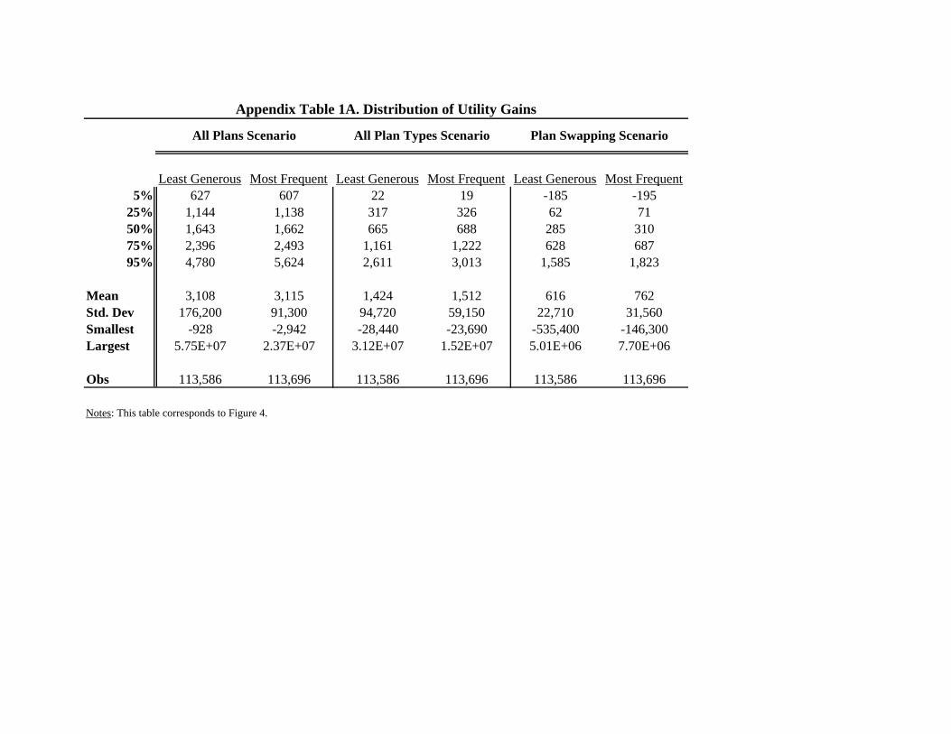
Least Generous Most Frequent Least Generous Most Frequent Least Generous Most Frequent5% 627 607 22 19 -185 -195

25% 1,144 1,138 317 326 62 7150% 1,643 1,662 665 688 285 31075% 2,396 2,493 1,161 1,222 628 68795% 4,780 5,624 2,611 3,013 1,585 1,823

Mean 3,108 3,115 1,424 1,512 616 762Std. Dev 176,200 91,300 94,720 59,150 22,710 31,560Smallest -928 -2,942 -28,440 -23,690 -535,400 -146,300Largest 5.75E+07 2.37E+07 3.12E+07 1.52E+07 5.01E+06 7.70E+06

Obs 113,586 113,696 113,586 113,696 113,586 113,696

Notes: This table corresponds to Figure 4.

Appendix Table 1A. Distribution of Utility Gains

All Plans Scenario Plan Swapping ScenarioAll Plan Types Scenario