Choice, Preferences and Utility

Mark Dean

Lecture Notes for Spring 2015 PhD Class in Decision Theory - Brown University

1 Introduction

The first topic that we are going to cover is the relationship between choice, preferences and utility

maximization. It is worth thinking about these issues in some detail as utility maximization is the

canonical model of behavior within economics. Even a lot of ‘behavioral’ models start with the

assumption that people maximize some sort fixed preference relation.

In your first year classes, you proved two fundamental results: Just as a reminder

Definition 1 Let A ⊆2∅ be a collections of choice sets, and : A→ 2∅ be a choice corre-

spondence. We say that a complete preference relation º rationalizes if, for any ∈ A

() = ∈ | º ∀ ∈

Theorem 1 For any finite set and complete choice correspondence : 2∅ → 2∅, there

exists a complete preference relation º that rationalizes that choice correspondence if and only if satisfies property and .

where

Axiom 1 (Property ) If ∈ ⊆ and ∈ (), then ∈ ()

Axiom 2 (Property ) If ∈ (), ⊆ and ∈ () then ∈ ()

1

Theorem 2 Let be a finite set. A binary relation º on has a utility representation if and

only if it is a complete preference relation.

These results are very powerful - they tell us what the observable implications of utility maxi-

mization are. However, they are also somewhat limited, in that they rely on quite strong assump-

tions. Specifically, they assume that

• We observe a complete choice correspondence - that is choices from every non-empty subset

of

• We observe a choice correspondence - so we get to see all the elements that a DM thinks is

best in a given set.

• is finite.

On can easily think of cases in which all three of these assumptions may fail. So the first thing

that we are going to do in this chapter is extend the results of theorems 1 and 2 to cover cases in

which we do not observe choices from every choice set, observe only a single choice, and in which

may not be finite (this last case is where things will get a little bit technical).

Here is a quick guide to some of the source materiel for this lecture if you want to learn more:

• “Notes on the Theory of Choice” by David Kreps gives a good, non-technical introduction tothe relationship between choice, preferences and utility in chapters 2 and 3

• “Real Analysis with Economic Applications ”by Efe Ok gives an extremely technical (but veryreadable) introduction to the same topic, and is the source you want if you are interested in the

details of the extension of our results to infinite spaces. Section A1 gives a good introduction

to order theory, while section B4 discusses ordinal utility theory

• “Lectures in Microeconomic Theory” by Ariel Rubinstein lectures 1 to 3 covers these issueswell, and also discusses some of the common failures of rationality

• The article “Consistency, Choice and Rationality” by Walter Bossert and Kotaro Suzumura(available on the web) goes through many of the issues in this chapter in extraordinary detail

• “Utility Theory for Decision Making” by Peter Fishburn is tough going, but contains almostall the key results in utility theory

2

2 What If We Do Not Observe Choices from Every Choice Set?

Theorem 1 assumes that we observe choices from every subset of the set . This is an extremely

strong assumption, as the number of choices that we have to observe gets very large very quickly

as the size of increases - if has elements, then we need to observe 2−1 choices. Given thatwe are often not going to have a data set that includes a complete choice correspondence, then a

natural question is whether we can drop the word ‘complete’ from the statement of the theorem.

In other words, if we observe a choice correspondence on an arbitrary subset of the power set of

does theorem 1 still hold? The answer is no, as the following example shows.

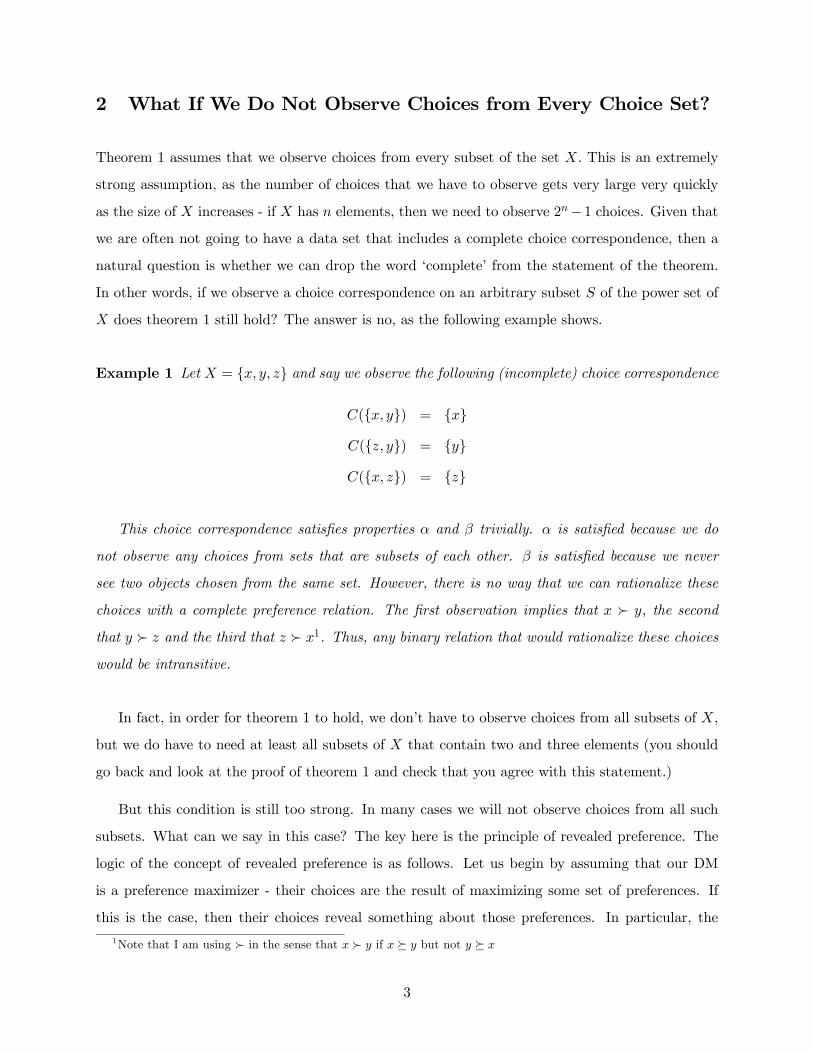
Example 1 Let = and say we observe the following (incomplete) choice correspondence

( ) =

( ) =

( ) =

This choice correspondence satisfies properties and trivially. is satisfied because we do

not observe any choices from sets that are subsets of each other. is satisfied because we never

see two objects chosen from the same set. However, there is no way that we can rationalize these

choices with a complete preference relation. The first observation implies that  , the second

that  and the third that  1. Thus, any binary relation that would rationalize these choices

would be intransitive.

In fact, in order for theorem 1 to hold, we don’t have to observe choices from all subsets of ,

but we do have to need at least all subsets of that contain two and three elements (you should

go back and look at the proof of theorem 1 and check that you agree with this statement.)

But this condition is still too strong. In many cases we will not observe choices from all such

subsets. What can we say in this case? The key here is the principle of revealed preference. The

logic of the concept of revealed preference is as follows. Let us begin by assuming that our DM

is a preference maximizer - their choices are the result of maximizing some set of preferences. If

this is the case, then their choices reveal something about those preferences. In particular, the

1Note that I am using  in the sense that  if º but not º

3

things that the DM chooses from as set must be the best elements in the set, according to the

preferences. Thus, if we see an object being chosen from a set, then we know that it is being

revealed preferred to all the other objects in that set. Note here that what we really mean is that

it has been directly revealed preferred, in the sense that it is at least as good as all the other

objects in the set. Furthermore, if we want our preferences to be transitive, then the fact that has

been revealed directly preferred to and revealed directly preferred to is enough to conclude

that is preferred to . Finally, if is chosen from some set while was available from the same

set and was not chosen, we would want to conclude that is strictly preferred to .

Definition 2 (The Principle of Revelaed Preference) Let be a choice correspondence on

a set . We say that is revealed directly preferred to if, for some ⊂ ∈ (), in

which case we write . We say that is revealed preferred to if there exists some sequence

1, 2,... ∈ such that

12

in which case we write . We say that is revealed strictly preferred to if, for some

⊂ , ∈ () and ∈ (), in which case we write

Is the principle of revealed preference a sensible one? Let us take the two concepts in turn.

First, the principle of weak revealed preference: is it sensible to say that if is chosen when is

available, then it cannot be the case that is preferred to ? I can certainly think of cases when

this is not a sensible assumption. For example, say that I am in a large wine shop, and I choose a

bottle to buy. Is this definitely my favorite wine in the shop? Almost certainly not, as I have not

searched through the entire wine shop. There may be a better wine out there that I have simply

not come across (we will deal with models that allow for this possibility in later lectures).

What about the principle of strict revealed preference? If anything, this is less convincing, as

it relies on the assumption that we observe a ‘choice correspondence’, which we never do in the

real world. All we ever get to see is the single object that a person actually chose. It is perfectly

possible that, in fact, they were indifferent between several alternatives, and selected one of those

from which they are indifferent, which would violate the principle of strict revealed preference.

Thus, in my opinion, it is best not to treat the principle of revealed preference as tautological

- if you chose over then you must prefer to . Instead, it is an implication of a model - the

4

model being that a DM’s choices are equivalent to the maximal elements in that set according to

their preference relation. From this observation we will be able to derive testable implications from

this model.

With that caveat aside, we now return to our problem. Just to be clear, our question is as

follows:

Problem 3 Let be a finite set, X ⊂ 2∅ be an arbitrary subset of the power set of and

be a choice correspondence on . Under what conditions is there a complete preference relation ºon that rationalizes ?

The answer is the Generalized Axiom of Revealed Preference

Definition 3 A choice correspondence satisfies the Generalized Axiom of Revealed Preference

(GARP) if, for any , ∈ such that it is not the case that

It turns out that GARP is necessary and sufficient for choices to be represented by a complete

transitive preference relation.

Theorem 4 Let be some non-empty set, and a choice function on A ⊆2∅. satisfies

GARP if and only if there exists a complete preference relation º that rationalizes

Proof. First, note that GARP implies directly that is the asymmetric part of . Second, note

that is the transitive closure of . Thus by Proposition 1 of the Order Theory notes there exisits

a complete preference relation º such that implies º and implies  . Thus

∈ ()

⇒ ∀ ∈

⇒ º ∀ ∈

5

and

∈ ()

⇒ ∃ ∈ s.t.

⇒ Â

⇒ 6º

so () = ∈ | º ∀ ∈

Proof. To show that the representation implies GARP, note that if choices are made in order to

maximize some complete preorder º, then implies that º and implies  , so

implies that there exists a chain 1, 2,... such that

º 1 º º Â

a contradiction.

Note that the theorem also does not require the finiteness of

What do we think of the weak cycles condition? From an aesthetic point of view, it is certainly

not as beautiful as conditions and - it all seems a bit mechanical and brute force - in a sense

the axioms seem to be stating the obvious. However, the flip side of this is that the OWC condition

is very easy to test, as we will discuss in the next lecture.

A few additional points to note

• Note that, if rather that observing a choice correspondence we observe a choice function, thenthe = . The GARP condition reduces to the requirement that is acyclic

• We might naturally want an equivalent relaxation of theorem 2. Let º be an arbitrary binaryrelation. Under what circumstances can we find a utility function such that º implies

() ≥ () and  implies () (). In fact, if we put together all the bits that we

have so far proved, we know the answer this question.

Theorem 5 Let be a finite, non-empty set, and º be a binary relation on and  and

∼ be the asymmetric and symmetric parts of º Then there exists a function : → R such

6

that

º implies () ≥ ()

 implies () ()

If and only if  ∼ satisfy OWC

Proof. First, note that, without loss of generality we can assume that ∼ is reflexive. If not,we can add the reflexive relations to º, and this will change neither whether or not º satisfies nor whether a particular function will represent º in the sense above.

Let be the transitive closure of º. OWC guarantees both that is an extension of º, andthat it cannot be that  . Thus, by theorem 4, there exists a complete preorder that

extends , and therefore º. By theorem 2 there exists a utility function that represents this

complete preorder and therefore º. That a utility representable binary relation satisfies OWCis trivial from the observation that º implies () ≥ () and  implies () ()

A couple of things to note. Firstly, in this case we DO need to be finite, as theorem 2 does

not necessarily hold otherwise. Second, note that the utility representation we have here is

worse that that of theorem 2. In that case, we could go both ways: we could construct the

preference relation from the utility function, or visa versa. That is not true in the case of

theorem 5. If all we know is the utility function, and we see that () ≥ (), then it could be

that , but it could be that the two are unrelated. For similar reasons, we can no longer

guarantee that is unique up to a strictly positive monotone transformation.

7

3 What If We Do Not Observe A Choice Correspondence?

Up until now, we have assumed that we can observe a choice correspondence - every choice set

maps to a subset. However, if you think about it for a minute, this should you make you feel

uncomfortable. A choice function is understandable - it is the thing that I observe you choose

from any given choice set. But what is this correspondence? It is not at all clear how to interpret

it. There are some suggestions in the literature - for example, if we observe a DM making choices

multiple times then we could call () the set of objects that we ever see chosen from , but

this seems to be unsatisfactory. If we are in a world where we observe multiple choices from people

which change from time to time, then surely we would want to model this explicitly? Perhaps by

thinking about the resulting distribution of choices? (we will come on to models that take this

approach later).

So can we drop the assumption that we observe a choice correspondence, and instead observe

a choice function? For example, we could ask the following question:

Question 1 Let : 2∅ → be a choice function. Under what conditions can we find a

complete preference relation º on such that

() ∈ ∈ | º ∀ ∈

In other words, under what conditions can we find a preference relation such that people always

choose one of the best available options.

Unfortunately, it should be pretty easy to see that we can always find such a complete preference

relation - we can just allow for everything to be indifferent! Then any object that the DM picks is

automatically one of the best. So this approach won’t get us very far.

Another thing we could do is just rule out indifference by assumption. In other words, we could

ask the following question.

Question 2 Let : 2∅→ be a choice function. Under what conditions can we find a linear

order  on such that

() = ∈ | Â ∀ ∈

8

In other words, under what conditions can we find a preference relation which does not allow

indifference such that people always choose the best available option.

Here we have solved the problem by assuming it away: by demanding that  is a linear orderwe can no longer explain behavior by allowing people to be indifferent between everything, because

we have ruled out indifference - in fact, we know that ∈ | Â ∀ ∈ is a singleton. In thiscase, it is simple to check that our previous theorems will go through: in the case of a complete

choice function the necessary and sufficient requirement is property ( is unnecessary) while in

the case of incomplete data, the necessary and sufficient requirement is OWC (though note that

this condition just becomes acyclicality in this case).

Is this a sensible approach? It certainly is not ideal: in general it seems possible that people

really are indifferent between two alternatives. If I am choosing between screwdrivers, I really don’t

care if the handle is blue or red. And if I am indifferent between the two, then it seems harsh to

declare me irrational because in some cases I choose the red handled one and in some cases the

blue handled one.

While there is no real agreed way out of this problem for general choice sets, we can do better

in the case of choices from budget sets. For this section, we will assume that the objects of choice

have a particular structure - that they are commodity bundles - there are commodities in the

word, and the DM has to select a bundle of these commodities, so ∈ is now

=

⎛⎜⎜⎜⎝1...

⎞⎟⎟⎟⎠where is the amount of good that is in the bundle. Choice sets are determined by a vector

of prices ∈ R+, giving a choice set ©

∈ R+|

ªIn this case our data will consist of observations of choices made from different price vectors indexed

. We will assume that income levels are not observed. We will denote by the bundle chosen

when price is in effect.

What does revealed preference mean in this context? Well, using the definition above, we say

that bundle is strictly revealed preferred over bundle if is chosen and is not when both

9

are available. If we see someone buy a bundle at prices , we know that the could have bought

any bundle which is cheaper that at prices . Thus we have

⇐⇒ ≤

However, this definition has all the attendant problems above: either we have to rule out

indifference by assumption, or we have to realize that we can potentially explain any pattern of

choices. To get round this problem, we can introduce a new, relatively innocuous assumption: that

people have preferences that are locally non-satiated.

Definition 4 A preference relation º on a commodity space R+ is locally non-satiated if, for any

∈ R++, 0 there exists some ∈ () such that  2

In other words, for any bundle there is another bundle close to such that is strictly preferred

to it. Is this a sensible assumption? Well, strictly monotonic preferences are locally non-satiated,

so if you believe that people in general like more stuff, then it may not be a bad assumption.

How does this help us? Well, it allows us to resurrect the concept of strict revealed preference,

even allowing for the possibility of indifference, and even in the case of choice functions. Consider

two bundles and such that . My claim is that, if our DM is choosing in order

to maximize a complete locally non-satiated preference relation (in the sense of question 1 above),

then it must be the case that Â

Lemma 1 Let and be two commodity bundles such that . Then, if the DM’s

choices can be rationalized by a complete locally non-satiated preference relation, then it must be

the case that Â

2Quick real analysis diversion. The notation () is the ’open epsilon ball around .’ In other words it is the set

of all objects that are a distance less than away from .

() = ∈ R|( )

where is some metric. As we are in R we can define the distance function

( ) =

=1

( − )2

10

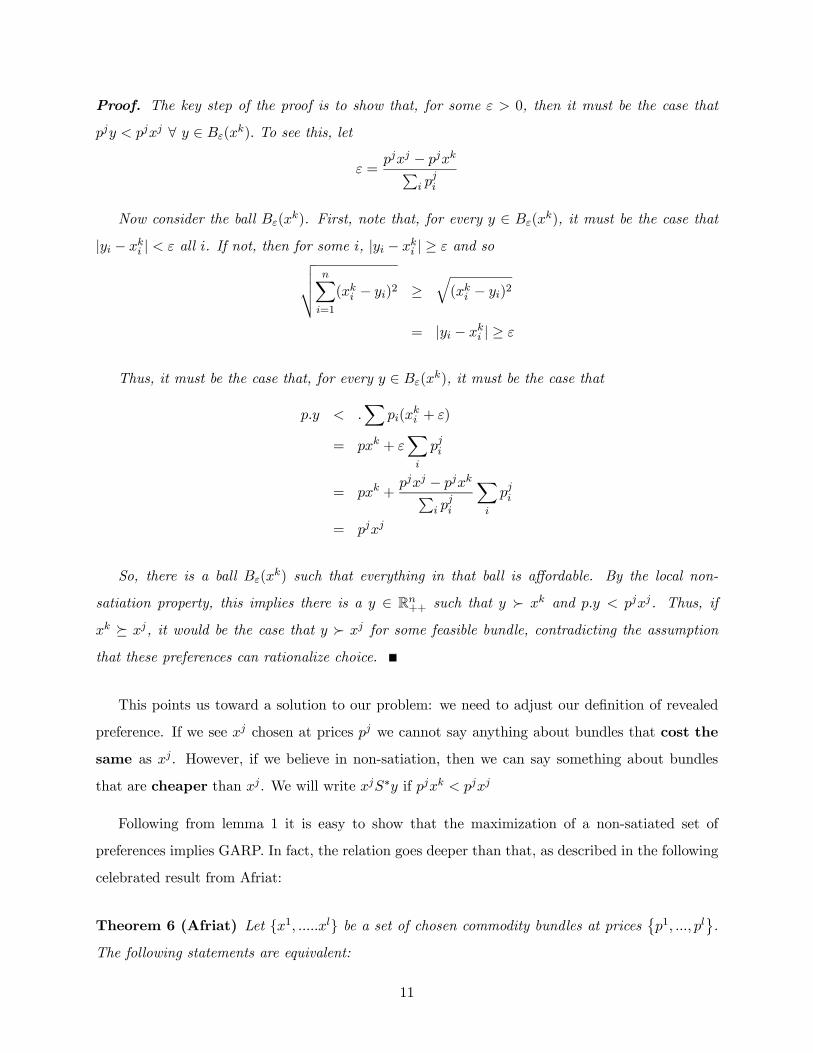
Proof. The key step of the proof is to show that, for some 0, then it must be the case that

∀ ∈ () To see this, let

= − P

Now consider the ball (). First, note that, for every ∈ (

), it must be the case that

| − | all . If not, then for some , | − | ≥ and sovuut X=1

( − )2 ≥q( − )2

= | − | ≥

Thus, it must be the case that, for every ∈ (), it must be the case that

X

( + )

= + X

= + − P

X

=

So, there is a ball () such that everything in that ball is affordable. By the local non-

satiation property, this implies there is a ∈ R++ such that  and . Thus, if

º , it would be the case that  for some feasible bundle, contradicting the assumption

that these preferences can rationalize choice.

This points us toward a solution to our problem: we need to adjust our definition of revealed

preference. If we see chosen at prices we cannot say anything about bundles that cost the

same as . However, if we believe in non-satiation, then we can say something about bundles

that are cheaper than . We will write ∗ if

Following from lemma 1 it is easy to show that the maximization of a non-satiated set of

preferences implies GARP. In fact, the relation goes deeper than that, as described in the following

celebrated result from Afriat:

Theorem 6 (Afriat) Let 1 be a set of chosen commodity bundles at prices ©1 ª.The following statements are equivalent:

11

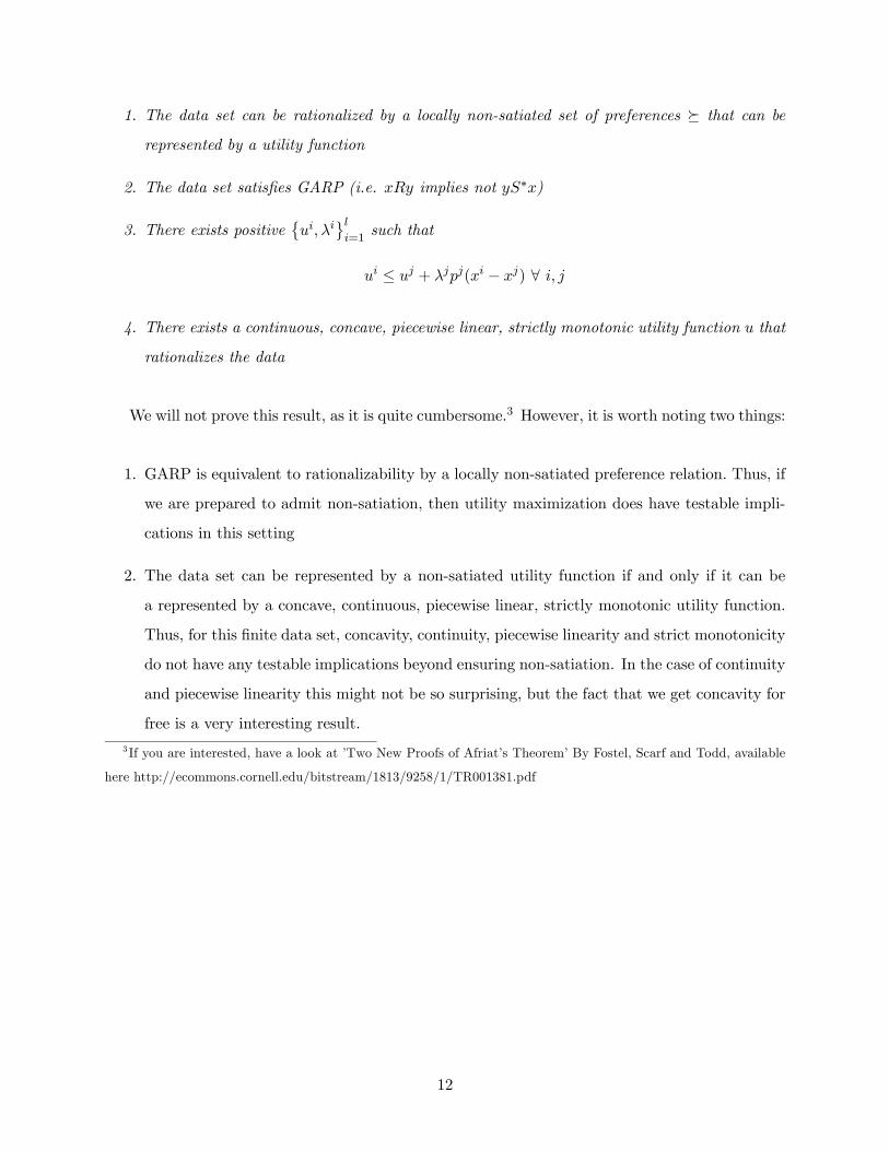
1. The data set can be rationalized by a locally non-satiated set of preferences º that can be

represented by a utility function

2. The data set satisfies GARP (i.e. implies not ∗)

3. There exists positive©

ª=1

such that

≤ + ( − ) ∀

4. There exists a continuous, concave, piecewise linear, strictly monotonic utility function that

rationalizes the data

We will not prove this result, as it is quite cumbersome.3 However, it is worth noting two things:

1. GARP is equivalent to rationalizability by a locally non-satiated preference relation. Thus, if

we are prepared to admit non-satiation, then utility maximization does have testable impli-

cations in this setting

2. The data set can be represented by a non-satiated utility function if and only if it can be

a represented by a concave, continuous, piecewise linear, strictly monotonic utility function.

Thus, for this finite data set, concavity, continuity, piecewise linearity and strict monotonicity

do not have any testable implications beyond ensuring non-satiation. In the case of continuity

and piecewise linearity this might not be so surprising, but the fact that we get concavity for

free is a very interesting result.

3 If you are interested, have a look at ’Two New Proofs of Afriat’s Theorem’ By Fostel, Scarf and Todd, available

here http://ecommons.cornell.edu/bitstream/1813/9258/1/TR001381.pdf

12

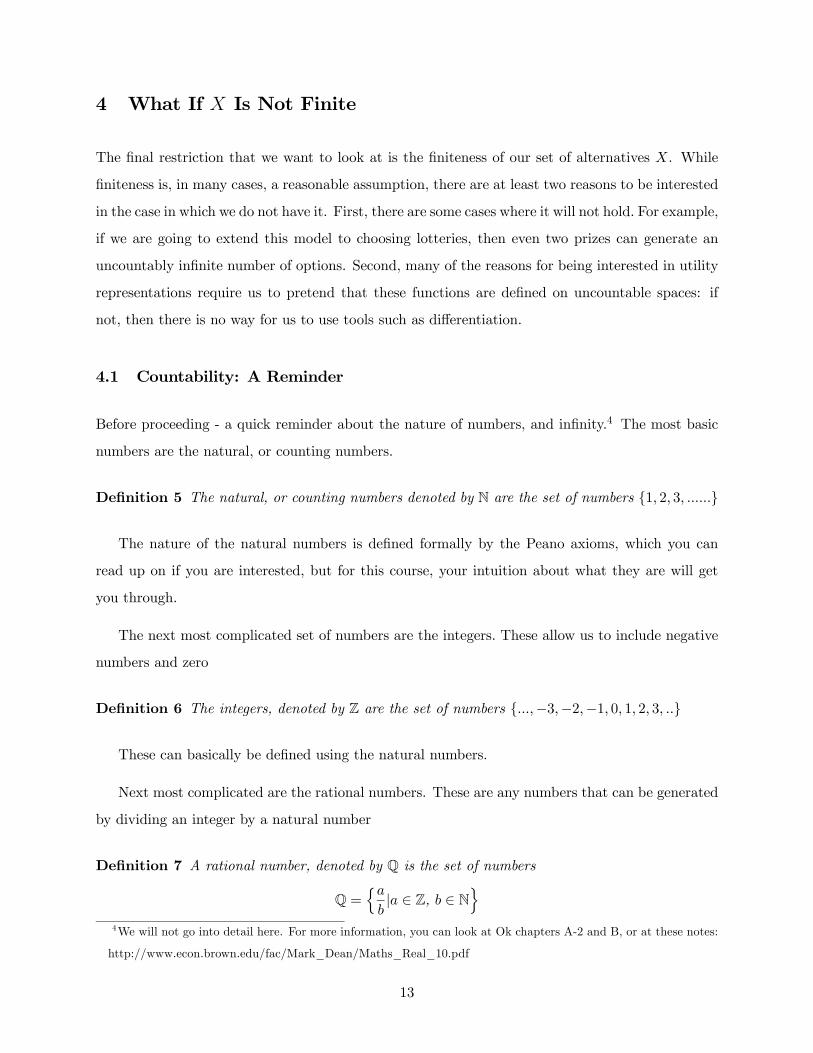
4 What If Is Not Finite

The final restriction that we want to look at is the finiteness of our set of alternatives . While

finiteness is, in many cases, a reasonable assumption, there are at least two reasons to be interested

in the case in which we do not have it. First, there are some cases where it will not hold. For example,

if we are going to extend this model to choosing lotteries, then even two prizes can generate an

uncountably infinite number of options. Second, many of the reasons for being interested in utility

representations require us to pretend that these functions are defined on uncountable spaces: if

not, then there is no way for us to use tools such as differentiation.

4.1 Countability: A Reminder

Before proceeding - a quick reminder about the nature of numbers, and infinity.4 The most basic

numbers are the natural, or counting numbers.

Definition 5 The natural, or counting numbers denoted by N are the set of numbers 1 2 3

The nature of the natural numbers is defined formally by the Peano axioms, which you can

read up on if you are interested, but for this course, your intuition about what they are will get

you through.

The next most complicated set of numbers are the integers. These allow us to include negative

numbers and zero

Definition 6 The integers, denoted by Z are the set of numbers −3−2−1 0 1 2 3

These can basically be defined using the natural numbers.

Next most complicated are the rational numbers. These are any numbers that can be generated

by dividing an integer by a natural number

Definition 7 A rational number, denoted by Q is the set of numbers

Q =n| ∈ Z, ∈ N

o4We will not go into detail here. For more information, you can look at Ok chapters A-2 and B, or at these notes:

http://www.econ.brown.edu/fac/Mark_Dean/Maths_Real_10.pdf

13

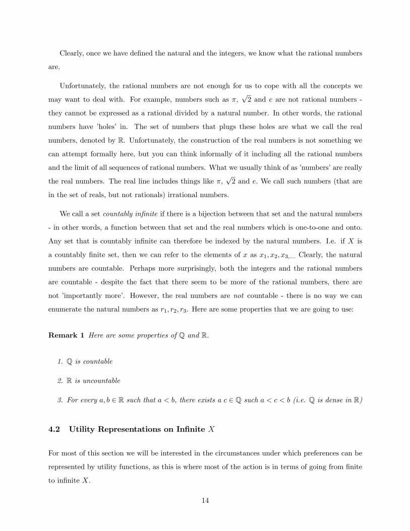
Clearly, once we have defined the natural and the integers, we know what the rational numbers

are.

Unfortunately, the rational numbers are not enough for us to cope with all the concepts we

may want to deal with. For example, numbers such as ,√2 and are not rational numbers -

they cannot be expressed as a rational divided by a natural number. In other words, the rational

numbers have ’holes’ in. The set of numbers that plugs these holes are what we call the real

numbers, denoted by R. Unfortunately, the construction of the real numbers is not something we

can attempt formally here, but you can think informally of it including all the rational numbers

and the limit of all sequences of rational numbers. What we usually think of as ’numbers’ are really

the real numbers. The real line includes things like ,√2 and . We call such numbers (that are

in the set of reals, but not rationals) irrational numbers.

We call a set countably infinite if there is a bijection between that set and the natural numbers

- in other words, a function between that set and the real numbers which is one-to-one and onto.

Any set that is countably infinite can therefore be indexed by the natural numbers. I.e. if is

a countably finite set, then we can refer to the elements of as 1 2 3. Clearly, the natural

numbers are countable. Perhaps more surprisingly, both the integers and the rational numbers

are countable - despite the fact that there seem to be more of the rational numbers, there are

not ’importantly more’. However, the real numbers are not countable - there is no way we can

enumerate the natural numbers as 1 2 3. Here are some properties that we are going to use:

Remark 1 Here are some properties of Q and R.

1. Q is countable

2. R is uncountable

3. For every ∈ R such that , there exists a ∈ Q such (i.e. Q is dense in R)

4.2 Utility Representations on Infinite

For most of this section we will be interested in the circumstances under which preferences can be

represented by utility functions, as this is where most of the action is in terms of going from finite

to infinite .

14

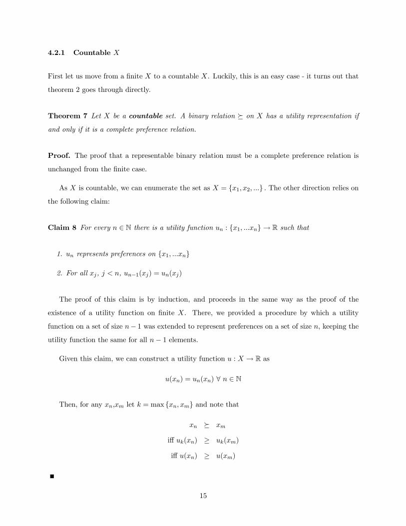
4.2.1 Countable

First let us move from a finite to a countable . Luckily, this is an easy case - it turns out that

theorem 2 goes through directly.

Theorem 7 Let be a countable set. A binary relation º on has a utility representation if

and only if it is a complete preference relation.

Proof. The proof that a representable binary relation must be a complete preference relation is

unchanged from the finite case.

As is countable, we can enumerate the set as = 1 2 The other direction relies onthe following claim:

Claim 8 For every ∈ N there is a utility function : 1 → R such that

1. represents preferences on 1

2. For all , , −1() = ()

The proof of this claim is by induction, and proceeds in the same way as the proof of the

existence of a utility function on finite . There, we provided a procedure by which a utility

function on a set of size − 1 was extended to represent preferences on a set of size , keeping theutility function the same for all − 1 elements.

Given this claim, we can construct a utility function : → R as

() = () ∀ ∈ N

Then, for any , let = max and note that

º

iff () ≥ ()

iff () ≥ ()

15

4.2.2 Uncountable

so can we extend the claim to cases where is uncountable. The answer is no, as the following

example demonstrates

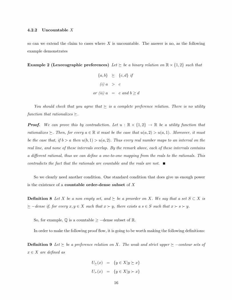
Example 2 (Lexecographic preferences) Let º be a binary relation on R× 1 2 such that

º if

(i)

or (ii) = and ≥

You should check that you agree that º is a complete preference relation. There is no utility

function that rationalizes º.

Proof. We can prove this by contradiction. Let : R × 1 2 → R be a utility function that

rationalizes º. Then, for every ∈ R it must be the case that ( 2) ( 1). Moreover, it must

be the case that, if then ( 1) ( 2). Thus every real number maps to an interval on the

real line, and none of these intervals overlap. By the remark above, each of these intervals contains

a different rational, thus we can define a one-to-one mapping from the reals to the rationals. This

contradicts the fact that the rationals are countable and the reals are not.

So we clearly need another condition. One standard condition that does give us enough power

is the existence of a countable order-dense subset of

Definition 8 Let be a non empty set, and º be a preorder on . We say that a set ⊂ is

º −dense if, for every ∈ such that  , there exists a ∈ such that   .

So, for example, Q is a countable ≥ −dense subset of R.

In order to make the following proof flow, it is going to be worth making the following definitions:

Definition 9 Let º be a preference relation on . The weak and strict upper º −contour sets of ∈ are defined as

º() = ∈ | º

Â() = ∈ | Â

16

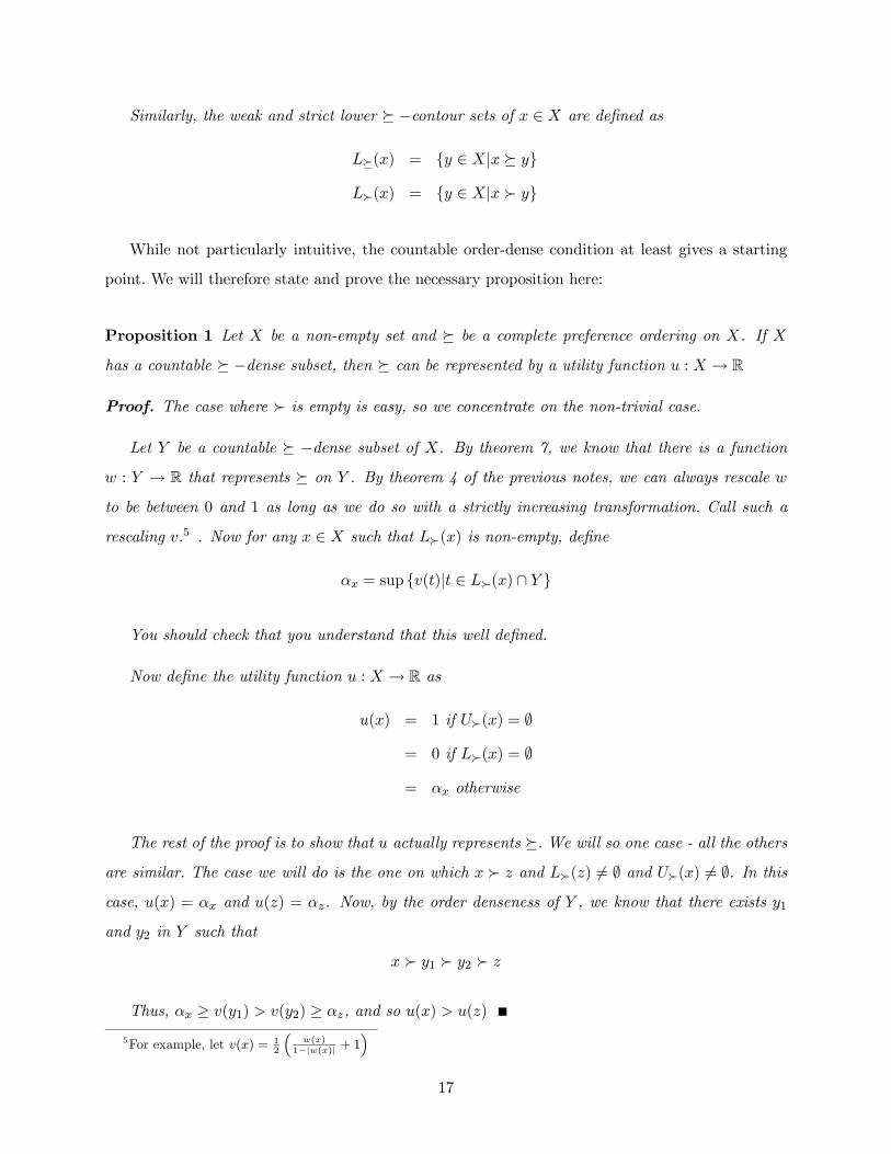
Similarly, the weak and strict lower º −contour sets of ∈ are defined as

º() = ∈ | º

Â() = ∈ | Â

While not particularly intuitive, the countable order-dense condition at least gives a starting

point. We will therefore state and prove the necessary proposition here:

Proposition 1 Let be a non-empty set and º be a complete preference ordering on . If

has a countable º −dense subset, then º can be represented by a utility function : → R

Proof. The case where  is empty is easy, so we concentrate on the non-trivial case.

Let be a countable º −dense subset of . By theorem 7, we know that there is a function

: → R that represents º on . By theorem 4 of the previous notes, we can always rescale

to be between 0 and 1 as long as we do so with a strictly increasing transformation. Call such a

rescaling .5 . Now for any ∈ such that Â() is non-empty, define

= sup ()| ∈ Â() ∩

You should check that you understand that this well defined.

Now define the utility function : → R as

() = 1 if Â() = ∅

= 0 if Â() = ∅

= otherwise

The rest of the proof is to show that actually represents º. We will so one case - all the othersare similar. The case we will do is the one on which  and Â() 6= ∅ and Â() 6= ∅. In thiscase, () = and () = . Now, by the order denseness of , we know that there exists 1

and 2 in such that

 1  2 Â

Thus, ≥ (1) (2) ≥ , and so () ()

5For example, let () = 12

()

1−|()| + 1

17

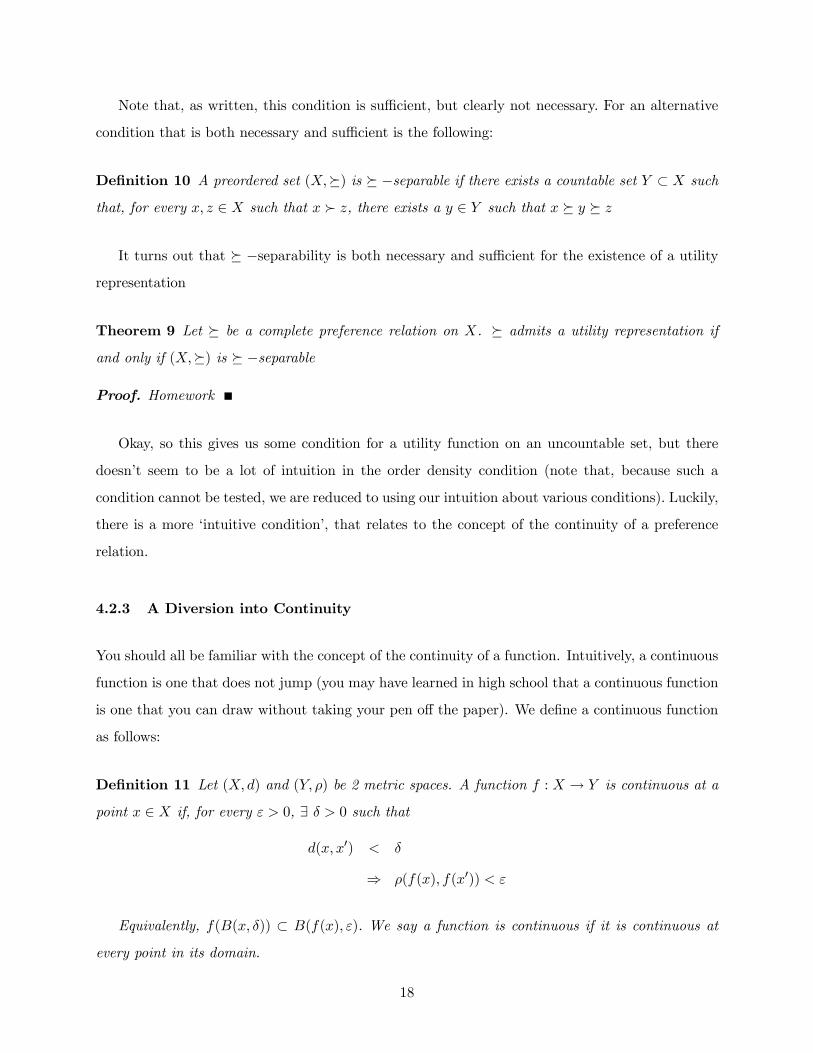
Note that, as written, this condition is sufficient, but clearly not necessary. For an alternative

condition that is both necessary and sufficient is the following:

Definition 10 A preordered set (º) is º −separable if there exists a countable set ⊂ such

that, for every ∈ such that  , there exists a ∈ such that º º

It turns out that º −separability is both necessary and sufficient for the existence of a utilityrepresentation

Theorem 9 Let º be a complete preference relation on . º admits a utility representation if

and only if (º) is º −separable

Proof. Homework

Okay, so this gives us some condition for a utility function on an uncountable set, but there

doesn’t seem to be a lot of intuition in the order density condition (note that, because such a

condition cannot be tested, we are reduced to using our intuition about various conditions). Luckily,

there is a more ‘intuitive condition’, that relates to the concept of the continuity of a preference

relation.

4.2.3 A Diversion into Continuity

You should all be familiar with the concept of the continuity of a function. Intuitively, a continuous

function is one that does not jump (you may have learned in high school that a continuous function

is one that you can draw without taking your pen off the paper). We define a continuous function

as follows:

Definition 11 Let () and ( ) be 2 metric spaces. A function : → is continuous at a

point ∈ if, for every 0, ∃ 0 such that

( 0)

⇒ (() (0))

Equivalently, (( )) ⊂ (() ). We say a function is continuous if it is continuous at

every point in its domain.

18

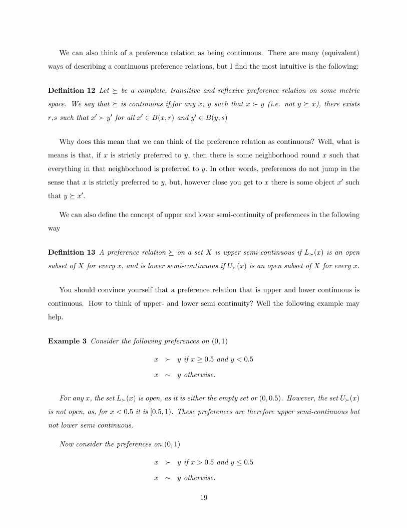
We can also think of a preference relation as being continuous. There are many (equivalent)

ways of describing a continuous preference relations, but I find the most intuitive is the following:

Definition 12 Let º be a complete, transitive and reflexive preference relation on some metric

space. We say that º is continuous if,for any , such that  (i.e. not º ), there exists

, such that 0 Â 0 for all 0 ∈ ( ) and 0 ∈ ( )

Why does this mean that we can think of the preference relation as continuous? Well, what is

means is that, if is strictly preferred to , then there is some neighborhood round such that

everything in that neighborhood is preferred to In other words, preferences do not jump in the

sense that is strictly preferred to , but, however close you get to there is some object 0 such

that º 0.

We can also define the concept of upper and lower semi-continuity of preferences in the following

way

Definition 13 A preference relation º on a set is upper semi-continuous if Â() is an open

subset of for every , and is lower semi-continuous if Â() is an open subset of for every .

You should convince yourself that a preference relation that is upper and lower continuous is

continuous. How to think of upper- and lower semi continuity? Well the following example may

help.

Example 3 Consider the following preferences on (0 1)

 if ≥ 05 and 05

∼ otherwise.

For any , the set Â() is open, as it is either the empty set or (0 05). However, the set Â()

is not open, as, for 05 it is [05 1). These preferences are therefore upper semi-continuous but

not lower semi-continuous.

Now consider the preferences on (0 1)

 if 05 and ≤ 05

∼ otherwise.

19

In this case, Â() is open but Â() is not for every . Thus, these preferences are lower but

not upper semi- continuous. This illustrates the notion that an USC preference relation is one that

may ‘jump’ down but does not jump up, while a LSC preference relation is one that may jump up,

but not down.

We can analogously define the concept of an USC and LSC function

Definition 14 A real valued function : → R is upper semi-continuous if, for every ∈ R, theset ∈ |() is open. It is lower semi continuous if the set ∈ |() is open.

One more thing we are going to need is the concept of a separable metric space. A separable

metric space is one that is ‘not too big’, in the sense that it contains a countable dense subset.

Definition 15 Let be a metric space. A set ⊂ is dense in if ( ) = A set is

separable if it has a countable dense subset.

The intuition is that a separable metric space is not ’too big’, as there is a countable space such

that each element of the base space is arbitrarily close to an element on the countable set. The

easiest example of a separable space is R. Can you show this?

One result that we will use, but not prove is the following:

Theorem 10 Let be a separable metric space,Then there exists a countable class O of open

subsets of such that

= ∪ ∈ O| ⊆

for any open set ⊂

4.2.4 Utility Representations with Continuity.

We will now discuss how the concept of continuity can help us guarantee the existence of a utility

representation, and in fact can guarantee the existence of a continuous utility representation. We

will do this by stating a set of lemmas. The first one we will prove, the later ones you will have to

take on trust.

20

Theorem 11 (Rader’s Utility Representation Theorem 1) Let be a separable metric space,

and º be a complete preference relation on . If º is upper (or lower) semi-continuous then it

can be represented by a utility function

Proof. By theorem 10, we know that there is a countable class O of open subsets of such that

= ∪ ∈ O| ⊆

for any open set ⊂ . Enumerate these sets O = 1 2 , and let

() = ∈ N| ⊆ Â()

And define

() =X

∈()

1

2

Notice that

º

⇐⇒ Â() ⊇ Â()

=⇒ () ⊇ ()

⇐⇒ () ≥ ()6

So the only thing we have to show is that () ⊇ () =⇒ Â() ⊇ Â(). To show this, take

such that Â() ⊇ Â() is false. This implies that there exists a such that ∈ Â() but

not ∈ Â(). As Â() is open, then there exists an open set that contains and is a subset of

Â(). But this set cannot be a subset of Â(), so () ⊇ () is false, so we are done.

In fact, we can say more, and Radner did. It turns out that, if the above conditions are met,

we can in fact represent the preferences with an upper semi continuous utility function

Theorem 12 (Rader’s Utility Representation Theorem 2) Let be a separable metric space

and º be a complete preference relation on . If º is upper (lower) semi-continuous then it can

be represented by an upper (lower) semi-continuous utility function

Proof. The theorem is provable for us, but it is tedious. If you are interested, have a look at Ok

section D.5.2

21

The daddy of theories such as this is Debreu’s representation theorem. This extends Radner 2

to tell us that continuous preference relations can be mapped to continuous utility functions

Theorem 13 (Debreu) Let be a separable metric space, and º be a complete preference rela-

tion on . If º is continuous, then it can be represented by a continuous utility function.

Proof. This cannot readily be proved with the tools that we have, but can be proved assuming a

result called the ’Open Gap Lemma‘. We will not do so, but if you are interested, look at Ok D.5.2

So far, we have not said anything about the link between choice and preference on uncountable

sets. To some extent there is not much to say - as we discussed before, properties and (or

OWC) are enough to guarantee rationalizability. However, there are two issues that we have not

looked into yet

1. Do all choices that result from maximizing a complete preference relation satisfy and ?

2. Given that continuity of º is important for utility representations, what conditions on choicedo we need to have them be rationalizable by a continuous preference relation?

The answer to the first question is clearly ‘no’, for the following simple reason: in general, for

infinite , the maximization of a preference relation may not even give rise to a choice function.

To see this, just consider the set = [0 1], and the preferences represented by º iff ≥ .

The set ∈ | º ∀ ∈ (0 1) is clearly empty.

Luckily there is an approach which will deal with both these issues. This approach is two-fold

1. We will consider only compact choice sets on metric spaces

2. We will define a continuous choice correspondence.

To do this, we need to define a metric on choice sets: what we want is for choices from choice

sets that are ’close’ to each other to also be close to each other. In order to make this formal, we

need some notion of closeness of sets. For this, we will use the Hausdorff metric:

22

Definition 16 (The Hausdorff metric) Let ( ) be a metric space, and () be the set of

all closed and bounded subsets of . We will define the metric space (() ), where is the

Hausdorff metric induced by , and is defined as follows: For any ∈ () define Λ() as

sup∈ (). Now define

() = max Λ()Λ()

Now we have defined a metric on closed and bounded sets, we can define the concept of a

continuous choice correspondence.

Definition 17 Let be a compact metric space and Ω be the set of all closed subsets of and

: Ω → 2 be a choice correspondence. If → for ∈ Ω , ∈ () ∀ and

→ , implies that ∈ (), then we say is continuous.

It turns out that continuity, plus and , is enough to give us our desired results

Theorem 14 Let be a compact metric space and Ω be the set of all closed subsets of and

: Ω → 2 be a choice correspondence. satisfies properties , and continuity if and only if

there is a complete, continuous preference relation º on that rationalizes .

Proof. For brevity, we will only prove the fact that continuity of choice correspondences implies

continuity of preferences. We know that it must be the case that

º iff ∈ ( )

You should also check, but the continuity of preferences is equivalent to the claim that, if → ,

→ such that º ∀ , then it cannot be the case that  . Now note that

Λ( ) = Λ( ) ≤ max ( ) ( )

so → in the Hausdorff metric. Also, if º ∀ , then ∈ ( ),then by continuity we have that ∈ ( ), and so not  .

23