LES of synthetic jets in boundary layer with laminar separation … · 2020-03-14 · LES of...
41
LES of synthetic jets in boundary layer with laminar separation caused by adverse pressure gradient Tetsuya Ozawa, Samuel Lesbros and Guang Hong* University of Technology, Sydney (UTS), Australia *Corresponding author. Mail address: Faculty of Engineering, University of Technology Sydney, PO Box 123, Broadway, NSW 2007, Australia. Email: [email protected] , Telephone: +61 2 9514 2678, Fax: +61 2 9514 2655 Abstract In the development of synthetic jet actuators (SJAs) for active flow control, numerical simulation has played an important role. In controlling the boundary layer flow separation, an integrated numerical model which includes both the baseline flow and the SJA is still in its initial stage of development. This paper reports preliminary results of simulating the interaction between a synthetic jet and a laminar separation bubble caused by adverse pressure gradient in a boundary layer. The computational domain was three-dimensional and Large-eddy simulation (LES) was adopted. The initial and boundary conditions were defined using or referring to our wind tunnel experimental results. Prior to numerically simulating the interaction between the synthetic jets and the baseline flow, a numerical model for simulating the separation bubble was developed and verified. In the numerical model including the SJA, the synthetic jet velocity at the exit of the SJA was defined as an input. The numerical model was further verified by comparing the simulation with experimental results. Based on reasonable agreement between the numerical and experimental results, simulations were carried out to investigate the dependency of flow control using synthetic jets on the forcing frequency, focused on the lower frequency range of the Tollmien-Schlichting (T-S) instability, and on the forcing amplitude which was represented by the maximum jet velocity at the exit of the SJA. Supporting the hypothesis based on the 1
Transcript of LES of synthetic jets in boundary layer with laminar separation … · 2020-03-14 · LES of...
LES of synthetic jets in boundary layer with laminar separation caused by adverse pressure gradient
Tetsuya Ozawa, Samuel Lesbros and Guang Hong*
University of Technology, Sydney (UTS), Australia *Corresponding author. Mail address: Faculty of Engineering, University of Technology Sydney, PO Box 123, Broadway, NSW 2007, Australia. Email: [email protected], Telephone: +61 2 9514 2678, Fax: +61 2 9514 2655
Abstract
In the development of synthetic jet actuators (SJAs) for active flow control, numerical simulation
has played an important role. In controlling the boundary layer flow separation, an integrated
numerical model which includes both the baseline flow and the SJA is still in its initial stage of
development. This paper reports preliminary results of simulating the interaction between a
synthetic jet and a laminar separation bubble caused by adverse pressure gradient in a boundary
layer. The computational domain was three-dimensional and Large-eddy simulation (LES) was
adopted. The initial and boundary conditions were defined using or referring to our wind tunnel
experimental results. Prior to numerically simulating the interaction between the synthetic jets
and the baseline flow, a numerical model for simulating the separation bubble was developed
and verified. In the numerical model including the SJA, the synthetic jet velocity at the exit of
the SJA was defined as an input. The numerical model was further verified by comparing the
simulation with experimental results. Based on reasonable agreement between the numerical and
experimental results, simulations were carried out to investigate the dependency of flow control
using synthetic jets on the forcing frequency, focused on the lower frequency range of the
Tollmien-Schlichting (T-S) instability, and on the forcing amplitude which was represented by
the maximum jet velocity at the exit of the SJA. Supporting the hypothesis based on the
1

experiment, LES results showed that the forcing frequency had stronger influence on SJA’s
effective elimination of the separation bubble than the forcing amplitude did.
Key words: synthetic jet actuator, micro sensor, numerical modeling, flow control.
Nomenclature
cP – pressure coefficient
Cs – Smagorinsky model constant
d0 – diameter of the orifice of the SJA
f – SJA’s forcing frequency
f - filtered value
F+ - non-dimensional frequency
G – filter function
Lx, Ly and Lz – dimension of the computational domains in the Cartesian directions x, y and z
N – sample size of experimental data
P(x) – pressure distribution in the streamwise direction
P - pressure parameter
ijS - strain tensor of grid-filtered velocity
t – time
ui – velocity in each of the three dimensions in Navier-Stokes equation, or the ith sample data
of the instantaneous streamwise velocity in Eq. (11)
u - sample mean of the streamwise velocity
uavg=0 – zero streamwise velocity at an averaged inflectional point
u’ – streamwise velocity fluctuation
u’max – maximum velocity fluctuation in the fluctuating velocity profile
2

iu , - sub-grid scale velocity ju
U – free stream velocity
ui – grid-filtered velocity
Ujet – jet velocity component in streamwise direction at the exit of SJA
Vjet – jet velocity component in direction normal to the wall at the exit of SJA
Wjet – jet velocity component in the spanwise direction at the exit of SJA
x – streamwise direction in the computational domain. x = 0 at the exit of the SJA.
xi, xj – space coordinates in Navier-Stokes equation
v – kinematic viscosity of the working fluid
ve – eddy viscosity
y – normal to wall direction in the computational domain
z – spanwise direction in the computational domain
ρ – density of the working fluid
τij – sub-grid scale stress
δ – boundary layer thickness
δ* - displacement thickness
Δ – width of the filter
θ – momentum thickness
1. Introduction
Despite many ‘unknowns’ in modeling the fluid flows, the challenge of CFD is now
compounded with the introduction of active flow control technologies [[28]]. In developing
synthetic jet actuators (SJAs) for active flow control, extensive work has been conducted on
numerical modeling of the synthetic jet generated in a quiescent external flow condition (in the
3

absence of a cross flow) [[11],[14],[17],[25]]. In this numerical modeling, the neighborhood of
the jet exit was simulated. Kral et al [[11]] aimed to model the boundary condition at the exit of
the orifice of the SJA. They did not model the air flow inside the cavity but examined three
different velocity distributions along the axial centerline of the orifice. They also investigated
various jets, laminar and turbulent, pulsed and steady, and achieved very good agreement
between the numerical simulation and the experimental measurement. The models in
[[14],[17],[25]] included the flow behavior in the cavity of the actuator and simulated not only
the jets generated but also the compression/intake and expansion/discharging processes in the
cavity.
Most of the reported work on numerical simulation of synthetic jets has been focused on the
jets in a quiescent condition. Few publications have reported numerical simulation of the
interaction between the synthetic jets and the baseline flow to be controlled. Mittal et al
simulated the synthetic jet at the exit of the SJA with cross flow in a boundary layer under a zero
pressure gradient [[17]]. Allan et al [[2]] investigated the numerical simulation of a 2-D airfoil
controlled by synthetic jets. They demonstrated the CFD model coupled with the model for rigid
body motion. Parekh et al [[20]] numerically simulated the experiments of Honohan et al [[10]]
that studied separation control on a thick airfoil using synthetic jet action. Their model
successfully predicted the reattachment dynamics and the dependence of controlling
reattachment on forcing frequency.
Different flow models and numerical approaches have been consistent in development and
enhancement through their applications. The turbulence models and solvers used in simulating
the synthetic jets in a quiescent condition include a two-dimensional incompressible flow model
with Reynolds-averaged Navier-Stokes (RANS) [[11]] or Direct Numerical Simulation (DNS)
4

[[17]], and three-dimensional model with DNS [[21]]. In the 2-D simulation of separation control
over an airfoil using synthetic jets, unsteady RANS [[2]] and hybrid RANS/LES derived from
combining the best features of RANS and LES [[20]] have been used.
Prior to numerically modeling the synthetic jets interacting with the baseline flow to be
controlled, it is necessary to have a numerical model ready for the baseline flow such as a
laminar separation bubble caused by adverse pressure gradient in the boundary layer. The
difficulties in modeling the separation bubble, especially the transition from laminar to
turbulence, have been well known. As commented by Gad-el-Hak [[3]], current inaccuracies in
turbulence modeling can severely degrade CFD predictions once separation has occurred. The
over-prediction of the production of turbulence kinetic energy and dissipation were reported in
[[22]]. However, while he pointed out the problems, Gad-de-hak also justified that the essence of
separation control was the calculation of attached flows, estimation of separation location, and
indeed whether or not separation would occur [[3]]. This has given us certain confidence in using
CFD as an alternative tool for developing synthetic jet actuators and also raised our cautiousness
for using CFD properly.
A closed region formed by laminar separation followed by turbulent attachment is known as a
laminar separation bubble. Laminar separation caused by adverse pressure gradient is a common
phenomenon in aerodynamic devices. Alam and Sandham reviewed the numerical simulation of
laminar separation bubbles from the first attempt in 1990 to 1998 [[1]], including LES used by
Wilson and Pauley to simulate two-dimensional large structures [[31]]. They commented that
only a few simulations provided good solution of the reattaching and developing turbulent
boundary layer.
5
Direct numerical simulation (DNS) of the incompressible Navier-Stokes equations was
applied to simulating the ‘short’ laminar separation bubble caused by adverse pressure gradient
in a boundary layer [[1],[23],[32]]. Alam and Sandham carried out simulations in both two- and
three-dimensions, and concluded that two-dimensional simulation failed to capture many of the
detailed features achieved from the three-dimensional simulation. They compared their
simulation results of transition length-based Reynolds number varying with local turbulence
level with the experimental ones, and showed good agreements. Rist used his DNS results to
give an introduction and an overview on instability and transition mechanisms in laminar
separation bubbles [[23]]. Regarding the numerical methods, Rist commented that RANS did not
cover the unsteady flow physics and LES was not yet well proven for transitional flow.
As reviewed above, although the numerical simulations of a synthetic jet in the absence of a
cross flow and of a separating boundary layer have been performed respectively, an integrated
numerical model including the synthetic jets in a separating boundary layer, is still being
developed. Rumsey summarized in 2008 that there had not been many published results for
computation of synthetic jet in a cross flow since the CFD workshop organized by NASA in
2004 [26]. Therefore, Work reported in this paper aimed to develop a three-dimensional LES
model which was reasonably capable of simulating the laminar separation bubble caused by
adverse pressure gradient, to provide a numerical baseline flow required for predicting the
effectiveness of a synthetic jet actuator (SJA) in controlling boundary layer flow separation.
2. Synthetic jet actuator
A synthetic jet, originated from the idea of acoustic streaming [[15]], has been known to have
zero-net-mass but non-zero momentum fluid flux generated by a device such as a piezo-
oscillator. It has emerged as a versatile actuator with potential applications ranging from
6

separation and turbulence control to thrust vectoring, and augmentation of heat transfer and
mixing [[3],[8],[12],[16],[30]]. A unique feature of synthetic jets is that they are formed entirely
from the working fluid of baseline flow without requirement of additional mass supply [[6]]. As
shown in the schematic in Fig. 1(a), a synthetic jet actuator consists of a cavity and an oscillating
diaphragm. The jet is synthesized by oscillatory flow through a small orifice to a cavity. The
flow is induced by a vibrating diaphragm which forms the bottom wall of the cavity.
Vortex rings
Oscillating diaphragm
d0
Cavity
(b) (a)
Figure 1 (a) Schematic diagram of a synthetic jet actuator (b) Instantaneous vortex contours of LES simulation of a synthetic jet in a quiescent condition
The synthetic jet actuator (SJA) in the present study used piezoelectric material for driving the
oscillating diaphragm, as it promotes desirable characteristics such as low power consumption,
fast response, reliability, and low cost [[6]]. As illustrated in Fig. 1(a), the SJA has an orifice in
the face opposite the membrane. This orifice is open to the boundary layer flow and has a
diameter, d0, of 0.5 mm. The actuator membrane is a thin circular brass disc, 0.25mm in
thickness, held firmly at its perimeter. A piezoceramic disc is bonded to the outside face of the
membrane. As specified by the manufacturer, the lowest resonant frequency of the membrane is
900 Hz and its lump sum capacitance is approximately 140 nF. In the wind tunnel experiments,
as shown in Fig. 1, the SJA was installed underneath a flat plate over which the streamwise
velocity was measured in a boundary layer developing under an adverse pressure gradient. In
7

operation, the SJA was driven by a sine wave signal generated by a standard electrical function
generator. An air jet was synthesized by oscillatory flow in and out of the cavity through the
orifice open to the boundary layer. As many other actuators for flow control, SJA tends to be a 2-
D excitation device. In Fig. 1(b) are the vortex contours from a 2-D LES simulation of the
synthetic jet in a quiescent condition. It shows the formation and development of the 2-D vortex
rings of the jet without cross-flow.
3. Experimental Background
The experiments investigating the synthetic jet actuator for controlling laminar separation
were performed in the low speed wind tunnel in the Aerodynamics Laboratory at the University
of Technology, Sydney. As shown in Fig. 2, in the working section, a fairing was set above an
aluminum flat plate with its angle adjustable for establishing the desired pressure gradient,
similar to that of a diffusion compressor blade. The flat plate, located 1200 mm from the working
section entrance, has a high quality surface finish. The leading edge of the upper surface is of
slender elliptical form and the plate has a 0.250 negative incidence to avoid leading edge
separation. Static taps were located every 25 mm along the streamwise centerline of the flat plate
for pressure measurement using a multi-tube manometer. The SJA was installed underneath the
flat plate and on the streamwise centerline. The exit of the SJA was an orifice open to the
boundary layer flow. The axial center of the orifice of the SJA was located 305 mm to the
leading edge. The streamwise velocity was measured using a Dantec hot wire anemometry in the
boundary layer flow over the upper surface of the flat plate. The ‘Streamline’ box in Fig. 2
shows a package of software and hardware for interfacing between the computer and the hotwire
probe and for data acquisition. The probe was traversed in streamwise (x) and normal (y)
directions. The sample rate was 6 kHz and the sample size of each realization was 4096.
8

Measurements were made at x = 40 ~ 160 mm downstream of the SJA (345 – 465 mm from the
leading edge) at 20 mm intervals. At each of the x stations, the hot wire probe was positioned at y
= 0.2 mm to beyond the edge of the boundary layer. At each measurement position, the
streamwise velocity was recorded in both conditions of jet on and off. The Reynolds number in
the measurement region, x = 40 ~ 160 mm, was in a range of 1.78x10⁵~2.24x10⁵. The forcing
voltage for the synthetic jets was ±7.5V, and forcing frequency 100 Hz. The freestream velocity
was 8.0 m/s and freestream turbulence was 0.5% measured at x = -50 mm which was the position
with the minimum pressure. More details about the wind tunnel tests are provided in [8,9].
Function generator
Synthetic jet actuator
Hotwire probe
Streamline Computer
U∞
x y
Figure 2 Side view of the experimental setting in the working section of the wind tunnel
4. Numerical Simulation
4.1 Computational domain
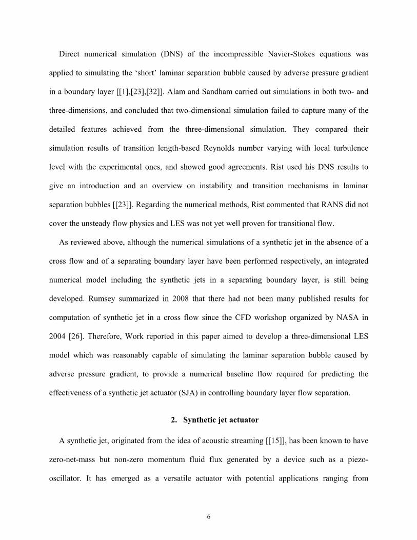
Figure 3 shows the computational domain. x corresponds to the streamwise direction, y the
wall-normal direction and z the spanwise direction. The bottom of the computational domain is
the upper surface of the flat plate in Fig. 2. To facilitate comparison with the experiments, the
dimensional length units are used. The dimensions of the computational domain are Lx = 200mm,
Ly = 60mm and Lz = 90 mm in streamwise, wall-normal and spanwise directions respectively.
9
The dimension in y direction was empirically set to be sufficiently high so that the velocity field
at the top of the domain was not to be influenced by the separation in the boundary layer at the
bottom of the computational domain. The domain is symmetric about the streamwise centerline
at z = 0. The reference position, x = 0, y = 0 and z = 0, is the axial centre of the orifice at the exit
of the SJA. The inlet of the computational domain is 20 mm upstream of the exit of the SJA,
defined as x = - 20 mm. In the course of developing this numerical simulation, it was noticed that
the shape of the SJA’s orifice, round or square, had insignificant effect on the simulation outputs.
Therefore, the round geometry of the orifice was replaced by a simple squared geometry in
simulation.
U
z
y
x
P(x)
Lx = 200 mm Lz = 45 mm
Ly = 60 mm
Vjet
Figure 3 Schematic of computational domain
(a)
10
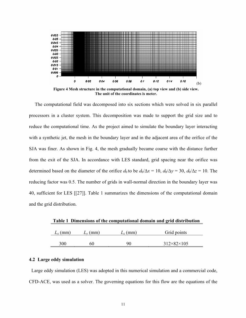
Figure 4 Mesh structure in the computational domain, (a) top view and (b) side view.
(b)
The unit of the coordinates is meter.
The computational field was decomposed into six sections which were solved in six parallel
processors in a cluster system. This decomposition was made to support the grid size and to
reduce the computational time. As the project aimed to simulate the boundary layer interacting
with a synthetic jet, the mesh in the boundary layer and in the adjacent area of the orifice of the
SJA was finer. As shown in Fig. 4, the mesh gradually became coarse with the distance further
from the exit of the SJA. In accordance with LES standard, grid spacing near the orifice was
determined based on the diameter of the orifice d0 to be d0/Δx = 10, d0/Δy = 30, d0/Δz = 10. The
reducing factor was 0.5. The number of grids in wall-normal direction in the boundary layer was
40, sufficient for LES [[27]]. Table 1 summarizes the dimensions of the computational domain
and the grid distribution.
Table 1 Dimensions of the computational domain and grid distribution
Lx (mm) Ly (mm) Lz (mm) Grid points
300 60 90 312×82×105
4.2 Large eddy simulation
Large eddy simulation (LES) was adopted in this numerical simulation and a commercial code,
CFD-ACE, was used as a solver. The governing equations for this flow are the equations of the
11

incompressible Navier-Stokes and the continuity equations. In LES, the velocity components in
the Navier-Stokes equations are decomposed into grid scale and sub-grid scale velocity, Ui+ ûi,
through the filter in space. Operationally, the filter is described as
___ 1( , ) ( ', ) ( ', , ) '2
T
fTx t f x t dtG x x t dx
Tf−
= −∫ Δ (1)
Where f represents the filtered value of the field variable, G denotes the filter which is a top hat
filter function. Δf is the filter width. The filtered Navier-Stokes and continuity equations become
as follows.
0
1
i
i
i i ij
j j i
ux
Du u pDt x x x x
τν
ρ
−
− −
∂ =∂
⎡ ⎤ ∂∂ ∂ ∂⎢ ⎥= −∂ ⎢ ∂ ⎥ ∂ ∂
⎣ ⎦
(2)
j
−
(3)
Where ij i jû ûτ = is the sub-grid scale (SGS) stress. Proposed methods for the closure of this term
are mainly categorized into two groups-eddy viscosity models and scale similarity models. CFD-
ACE provides the SGS Eddy Viscosity Coefficient model in which the SGS stress term is
defined as:
ijeij Sv−≈τ (4)
⎟⎟⎠
⎞⎜⎜⎝
⎛
∂∂
+∂∂
=i
j
j
iij
xu
xu
S21 (5)
Where νe is the SGS eddy viscosity and ijS is the strain tensor of grid-filtered velocity.
Smagorinsky model based on isotropy-of-the-small-scales assumption has been broadly used due
to its simplicity and accuracy [[29]]. Although the simulation of a homogeneous isotropic
turbulence using Smagorinsky model may agree well with the experiment, SGS model does not
12

have the versatility for various flow fields including the one in the present study. Thus, the
Dynamic SGS model [[13]] was considered.
4.3 Initial and boundary conditions
The mean freestream velocity components at the inlet of the computational domain were
defined as U = 9.1 m/s (x-direction), V = 0 m/s (y-direction) and W = 0 m/s (z-direction). Since
the velocity profile at the inlet of the computational domain was not measured in the
experiments, the numerical modelling of the inlet flow was required. A Blasius velocity profile
of a laminar boundary layer was assumed at the inlet of the computational domain. The free
stream mean velocity at the inlet was adjusted by the boundary layer thickness based Reynolds
number Reδ, of approximately 500. Artificial-minute disturbance at the inlet was adopted by
generating Gaussian Random numbers. The root-mean-square (RMS) of the disturbance was 1%
of the free stream velocity at the inlet. It was determined based on justifying the positions of the
separation and reattachment points and the bubble length [[19]].
In the work reported in [[18]], convective boundary condition was used at the exit of the
computational domain. An artificial ‘buffer’ zone was employed at the end of the computational
domain to return the turbulent outflow to the Blasius laminar inflow profile, in order to apply
periodic boundary conditions in the streamwise direction in the use of a fully spectral method. In
our work, the outlet boundary condition of the computational domain was defined by the
pressure value measured at the streamwise position of x =180mm in the wind tunnel test.
The condition at the top boundary of the computational domain in [[18]] was defined by a
suction (normal) velocity profile Vtop(x) with a Gaussian distribution. By doing so, the
separation and the reattachment points were fixed. Alternatively the entire wind tunnel was
included in the model [[32]]. However, fixing the positions of the separation and reattachment
13

does not suit the present study, as effective synthetic jets modify the separation and reattachment
points. Instead of the velocity profile defined at the upper boundary of the domain, a pressure
profile was applied with the following function.
)(),,,( xPtzLxP topy = (6)
Where P is the static pressure as a function of the location and time. The setting of the models’
height (in wall-normal direction) in this simulation was extensively examined and carefully
decided [[19]]. The pressure coefficient from the experimental measurement, as shown in Fig. 5,
was imposed onto the top boundary of the computational domain. In doing so, the free stream
velocity and the adverse pressure gradient resulting in the boundary layer separation were
defined in the LES model.
The non-slip boundary condition was set on the bottom wall of the computational domain
with zero velocity defined at the wall y = 0. The flow at the side walls of the computational
domain was assumed to be symmetric about z = 0. Applicable to both sides of the center, the
symmetric boundary conditions generate a flow of period length 2×Lz.
-0.80
-0.60
-0.40
-0.20
0.00
-0.020 0.030 0.080 0.130 0.180x (m)
Cp
Figure 5 Static pressure distribution in the downstream direction
4.5 Numerical Method
14

By filtering the Navier-Stokes and the continuity equations in space, grid-filtered governing
equation and Sub-grid scale stress (SGS) terms were produced. Dynamic Smagorinsky model
was used for the approximation of SGS stress terms. Filtered Equations (2) and (3) were
discretised in space using a hybrid scheme of the second-order central difference and first order
upwind difference. 2,686,320 grid points were used, consisting of the concentrated mesh near the
wall and the orifice of the SJA. ΔY+ at the first node off the wall in the boundary layer was less
than 0.6, and the corresponding ΔX+ was less than 19 and ΔZ+ less than 50. To test the grid
independence, the mesh was refined with decreased ΔX+ and ΔZ+. The characteristic parameters
as the output showed insignificant difference with the finer mesh.
The forward and backward Euler and the second-order Crank-Nicolson methods were
employed for time integration. The time step was set as Δt = 0.0002s and the total number of
time steps was 1600 in each run. The time step was set based on the forcing frequency of the SJA
and the sample rate for data acquisition, 6 kHz, in the experiments. The simulation began at time
t = 0, with an analytical approximation to the steady-state solution. The flow was considered as
transient and the residual convergence was less than 10-3. The CPU time for one simulation was
about 36 hours for 500 time steps.
5. Simulation of Laminar Separation Bubble
In the development of the baseline flow model, a laminar separation bubble was formed in the
boundary layer. Sample results are presented in the following sections to identify the separation
bubble and to analyze the mechanics associated.
5.1 Laminar Separation-Short Bubble
15

Flow separation can be transitional separation or laminar separation, depending on the flow
mode before the separation occurs. In order to identify the separated-flow transition modes,
Hatman and Wang developed a prediction model for distinguishing three separated-flow
transition modes, transitional separation, laminar separation-short bubble and laminar separation-
long bubble [387]. The transitional separation has the onset of the transition occurring upstream
of the separation point, and the other two have the onset of the transition downstream of the
separation point by inflectional instability. In separated boundary layers, the model proposed by
Hatman and Wang for separated-flow transition is based on the assumption that the transition to
turbulence is a result of the superposition of the effects of two different types of instability:
Kelvin-Helmholtz (K-H) instability and Tollmien-Schlichting (T-S) instability. The
predominance of one type of instability determines the modes of separated-flow transition.
Laminar separation-short bubble was the one identified in our experimental studies [[8]] and
simulated in our numerical studies [[19]]. It distinguishes itself from the transitional separation
and the laminar separation-long bubble by a quick completion of transition. The laminar
separation-short bubble mode occurs at moderate Reynolds numbers and mild adverse pressure
gradients. The onset of the transition is induced downstream of the separation point by
inflectional instability at a location coincidental with that of the maximum displacement in the
shear layer. It is characterized by a quick transition completion due to a complex interaction
between the separated shear layer and the reverse flow vortex. After the laminar shear layer
detaches, the K-H instability sets in. The onset of the transition from laminar to turbulence
should be situated close to the location of the maximum bubble elevation [[7]]. Then a short
early transition region takes place. This early transition is shortened by a periodic ejection of
turbulent fluid from the recirculating region into the detached shear layer. Instability waves of
16

the T-S type, initiated upstream of the separation point, may still be present within the detached
shear layer. The coalescence into turbulence takes place within the reattaching boundary layer,
resulting in a short late transition region.
5.2 Visualization of the separation bubble
0.0
0.2
0.4
0.6
0.8
1.0
1.2
1.4
0 20 40 60 80 100 120 140 160
x (mm)
y (m
m)
(1) (2) (3) (4)
X S X MD, X T X R, X u'max
Figure 6 Laminar separation-short bubble viewed by positions with uavg = 0, on z = 0 plane
Figure 6 shows the laminar separation-short bubble on the streamwise centerline from the
LES simulation. The ‘edge’ of this separation bubble is viewed by the averaged positions with
zero streamwise velocity, uavg=0, which exists in an inflectional velocity profile. Here XS is the
streamwise position of the separation point. XMD is the streamwise position with the maximum
displacement. XT is the onset of the transition from laminar to turbulence, XR is the streamwise
position of the reattachment and Xu’max is the streamwise position with the maximum fluctuating
velocity. The separation (XS) occurs at about x = 41mm and the flow reattaches to the wall (XR)
at about x = 134mm. The transition onset (XT) occurs at about x = 110 mm. In region (1) is
attached laminar flow. In region (2) is laminar shear layer detached from the wall. The
streamwise length of region (2) is 77% of the bubble length. For a laminar separation-short
bubble, the onset of the transition from laminar to turbulence, XT, occurs at a position
17

coincidently with the maximum displacement (XMD) [7]. The transition from laminar to turbulent
is characterized by a short early transition region which is region (3) between [XMD, XT] and [XR,
Xu’max]. The length of region (3) is 23% of the bubble length. In region (3), the mid-transition
point (Xu’max) is merged with the reattachment point, XR. In region (4) is the developing turbulent
flow after reattachment.
0.01
0.1
1
10
0 20 40 60 80 100 120 140 160 18
x (mm)
u'm
ax (m
/s)
0
Separation point
Reattachment point
Figure 7 Variation of the maximum fluctuating velocity u’max on streamwise centerline
For a laminar separation bubble in a short mode, caused by relatively moderate adverse
pressure gradient, the vigorous mixing in the region of the maximum fluctuating velocity, u’max,
leads to reattachment [7]. The development of the ‘maximum fluctuating velocity’ along the
streamwise centerline is shown in Fig. 7. Note that this ‘maximum fluctuating velocity’, u’max, is
the maximum in the fluctuating velocity profile at a streamwise position. As shown in Fig. 7,
u’max remains constant up to the position about 20 mm upstream of the separation point. Inside
the separation zone, u’max increases exponentially until it reaches the position close to the
reattachment point. The peak value of u’max occurs at the reattachment point about x = 134mm.
This shows one of the characteristics of a laminar separation-short bubble that the turbulence
level is maximum at the reattachment, as reported in [738]. This result is also consistent with that
18

of the DNS of a laminar separation bubble in [[24]]. The cause of this rapid increase can be
explained as that the disturbance at the inlet is amplified by the Kelvin-Helmhortz (K-H)
instability in the free shear layer flow. After the reattachment point where the peak value of u’max
is reached, the flow quickly becomes turbulent, as shown by the decrease of the maximum
fluctuating velocity in Fig. 7.
5.3 Transition from laminar to turbulent
Simulation results in Figures 6 and 7 show that the laminar separation bubble, including the
separation point and the re-attachment, was well captured. However, questions remain for the
capability of this LES model to simulate the transition from laminar to turbulent. Vorticity may
be used to identify the mixing between the sub-layer and the rest of the boundary layer. Figure 8
presents the iso-surface of the instantaneous vorticity of 2000 near the wall. Note that the
distance is in the unit of meter and the spectrum bar gives the scale of the time averaged
streamwise velocity. As shown in Fig. 8, the mixture starts to be enhanced at about x = 110 mm,
where the flow is still separated. Following this, the re-attachment occurs very quickly. It can
also be observed that the large-scale waves transfer in streamwise direction and the laminar layer
breaks down into streak structure downstream, similar phenomenon as described in [[1]]. After
the reattachment occurs at about x =134 mm, the flow structure becomes finer and more
complicated. Further downstream, the turbulence level increases quickly.
19

Figure 8 Iso-surface of instantaneous vorticity of 2000 (The spectrum bar shows the scale of the mean streamwise velocity)
0
2
4
6
8
10
12
14
0 2 4 6 8
u (m/s)
y (m
m)
10
ExperimentLESBlasius
Figure 9 Mean velocity profiles at x = 160 mm, compared with Blasius velocity profile
To identify the flow condition downstream of the reattachment, the mean streamwise velocity
profiles at x = 160 mm are examined. In Fig. 9, the numerical and experimental results of the
mean streamwise velocity profiles at x = 160mm are compared, and they are also compared with
the Blasius profile. It shows a good agreement between the experimental and numerical results
for the mean streamwise velocity profiles at this position which is downstream of the
20

reattachment. The shape factor H1 values at this position are 1.775 from the experiment and
1.672 from the simulation. Compared with the Blasius velocity profile, the ‘fuller’ velocity
profiles in both experiment and simulation indicate that the flow is turbulent at x = 160 mm. The
results shown in Figures 6-9 demonstrate that LES is reasonably capable of capturing the major
features in the baseline flow which includes the laminar separation and the transition from
laminar to turbulent in a boundary layer at an adverse pressure gradient.
5.4 Model Verification
The numerical simulation of the laminar separation bubble is verified by experiment. Results
of the mean and fluctuating velocity profiles, the bubble length and the pressure distribution will
be compared between the LES simulation and the wind tunnel experiment.
Figure 10 shows the comparison of the mean and fluctuating velocity profiles at z = 0 in the
separation region obtained from the experiment and the numerical simulation, noting that hot
wire measurements can not give the sign of the velocity. The mean velocity is the sample mean
of the instantaneous streamwise velocity normalized by the velocity of the local potential flow.
The fluctuating velocity, u’, was calculated as follows.
u′ = N
uuN
ii∑
=
−1
2)( (7)
Where ui is the ith sample data of the instantaneous streamwise velocity, u is the mean of the
streamwise velocity, and N is the sample size of one realization.
Both numerical and experimental results in Fig. 10(a) show consistently the inflection points
in the velocity profiles at y positions close to the wall in the region of x = 40~120 mm, indicating
a separation region. In the same separation region, the fluctuating velocity shown in Fig. 10(b) is
small, further indicating that it is a laminar separation. Both numerical and experimental results
21

in Fig. 10 also consistently show that the reattachment occurs at a position between x = 120 and x
= 140 mm, and that the mean velocity profiles are characterized by turbulent boundary layer, at x
= 160 mm. The similar variation of the mean and fluctuating velocity profiles positively support
the verification of the LES model.
0
2
4
6
8
10
40 60 80 100 120 140 160 180x (mm)
y (m
m)
(a)
0
2
4
6
8
10
20 40 60 80 100 120 140 160 180x (mm)
y (m
m)
(b)
Figure 10 Velocity profiles in the separation region along the streamwise direction without SJA (a): Mean velocity, u/U, (b): Fluctuating velocity u’/U. -- Numerical simulation, ° Experiment.
The difference, however, between the numerical and experimental results shown in Fig. 10 is
obvious, especially in the transition region of x = 100~140 mm. The inviscid K-H instability,
starting upstream of the position x = 40 mm, develops more quickly in the numerical simulation
22

than in the experiment. In the transition from laminar to turbulence, the numerical fluctuating
velocity is characterized by stronger development of frictional instability and greater than the
experimental one. When the boundary layer flow becomes more steady at x = 160 mm, the
difference between the numerical and experimental results is significantly reduced. The
difference between the numerical simulation and experiment could be caused by the assumed
Blasius velocity profile at the inlet of the computational domain and the freestream turbulence
level higher in the numerical simulation than that in the experiment.
Figure 11 Separation region shown by the zero mean streamwise velocity uavg = 0.
(The dimensions are in meter)
The iso-surface of the inflectional points with zero streamwise velocity uavg = 0 is used to
visualize the shape and dimensions of the separation bubble, as shown in Fig. 11. The minimum
and maximum x positions with uavg = 0 are used to approximate the separation point and the
reattachment points respectively. The separation point on the streamwise centerline occurs at x =
41mm and the re-attachment occurs at about x = 134 mm. The corresponding bubble length is
93mm. Note that the x positions for separation and reattachment points were obtained by
averaging respectively the first and the last x positions with uavg = 0. As observed in the
development of this numerical model, the separation location was well identified at x = 41mm, as
the onset of the separation point consistently occurred at the same x position. However, in the
23

breakdown region (x =120mm~140mm), the reattachment position was varying from one
simulation to another. Consequently, a fixed reattachment point could never be reached. This
experience is actually in good agreement with that in [[22]]. Compared with the bubble length
which was in the range between 60 and 100mm in the wind tunnel tests, the numerical result of
the bubble length of 93 mm is within the range of the experimental result.
Figure 12 compares the experimental and numerical results of pressure distribution in the
streamwise direction. As agreed in both experimental measurement and numerical simulation,
the pressure distribution is quite ‘flat’ from x = 40mm and x = 110 mm, followed by a quick
increase before the pressure gradient is recovered around x = 140mm. The zone with the ‘flat’
pressure distribution is where the laminar separation bubble exits. Gaster [[5]] proposed a two-
parameter bubble criterion by means of a relationship between the Reynolds number at
separation which was based on the momentum thickness θ, and the variation of the free stream
velocity over the separation zone. This relation can be described by equation (8).
xUP
ΔΔ=
νθ 2
(8)
Where P is pressure parameter, is the variation of the free stream velocity over the bubble,
and is the bubble length. Based on the momentum thickness and the drop of the free stream
velocity in the separation region obtained numerically and experimentally, the corresponding Re
UΔ
xΔ
θ
and P are 300 and -0.14 respectively. In accordance with Gaster’s criterion, the separation in the
present study is identified as short-bubble separation. This also confirms the height in wall-
normal direction of the computational domain, as the short bubble has no influence to the free
stream.
24

-0.8
-0.6
-0.4
-0.2
0.0
0 50 100 150 200
x (mm)
Cp
Experiment
LES
Figure 12 Pressure distributions on the flat plate along the streamwise direction
5.5 Influence of total time steps
With a fixed time step, the total number of time steps in a certain time length was numerically
tested to decide the minimum number of time steps required for one simulation. If the output
parameter, for example the mean velocity profile, does not change significantly with increased
total number of time steps, the simulation is regarded converged towards a single solution and
the minimum number of time steps should be selected. Figure 13 compares the mean velocity
profiles at seven streamwise stations, simulated with total numbers of time steps of 800 and 1600
respectively. It shows that the difference in this major output from simulations with two different
total numbers of time steps is insignificant.
25

x (mm)
y (m
m)
40 60 80 100 120 140 160
14
12
8
4
Figure 13 Comparison of mean velocity profiles computed with different time steps.
Dashed line: 800 time steps, Solid line: 1600 time steps
However, significant differences exist in other output from the same simulations. Table 2
shows the positions of the separation and reattachment points from two simulations with total
time steps of 800 and 1600, compared with the experiment. The separation point appears earlier
and the reattachment point does later with 800 time steps than that with 1600 time steps. As a
result, the bubble length with 800 time steps is 10% longer than that with 1600 time steps. The
separation bubble with 800 time steps is also outside the range of the bubble length obtained
from the experiment. Compared with the experimental results, the positions of separation and
reattachment points and the bubble length with 1600 time steps agree well with the experimental
results. 1600 time steps were therefore adopted in the simulations.
Table 2 Influence of computational time steps on the separation bubble
Separation point x (mm)
Reattachment point x (mm)
Bubble length (mm)
800 time steps 36 138 102
1600 time steps 41 134 93
Experiment 40-60 120-140 60-100
26

6. Simulation with SJA
In the present numerical simulation with the SJA installed, the cycle involving compression
and expansion processes in the cavity of the SJA was not simulated. Instead, the velocity along
the centreline of the orifice of the synthetic jet was defined as an inlet to the computational
domain at the exit of the SJA. The jet velocity was assumed to be a sine function of time in the y
direction, and defined as
Ujet = 0
(9) Vjet = Vjet,max sin (2π f t)
Wjet = 0
Where Ujet and Wjet are the jet velocity values in the streamwise (x) and spanwise (z) directions
respectively, and Vjet is the jet velocity along the axial centreline of the orifice in the normal (y)
direction. Vjet,max is the amplitude of the sine function. f is the forcing frequency and t is the time.
The first assumption here is that the outlet flow along the axial centreline of the orifice of the
SJA is a function of time and a sine wave without consideration of the phase change. It is
possible in a real flow that the phase and/or the profile of the jet velocity would vary with time.
The second assumption is that the synthetic jet be unaffected by the constriction at the orifice
based on our experimental investigation [[8]]. Therefore, the round shape of the orifice of the
SJA is replaced by a squared one in the numerical model. The third assumption is that the
fluctuating component of the jet velocity be ignored. Figure 2 shows the location of the jet
velocity defined as an input in the computational domain. Consistently located as in the
experiment, the centreline of the orifice of the SJA in the numerical simulation is on the
streamwise centreline of the flat plate and 20mm from the inlet of the computational domain. In
the 3-D coordinates, the jet velocity was defined at x = 0, y = 0 and z = 0.
27

Based on our experimental results [[9]], the non-dimensional frequency F+ =∞Uxf of the
baseline flow was calculated to be in a range of 0.72~1.41. In this calculation, the forcing
frequency, f, was 100 Hz. The length of the laminar separation bubble, x = 60~100mm, was
taken as the characteristic length and the freestream velocity U∞ was the velocity of the local
potential flow. To sufficiently cover the frequency components in the simulation, the time step
was set at Δt = 0.0002 second, so that the sine wave with a frequency of 100 Hz could be
numerically sampled by 50 time steps. The simulation of the baseline flow without SJA was run
until an equilibrium flow state was reached. The equilibrium flow state then served as the initial
conditions for the simulations with the SJA.
7. Verification of model with SJA
Figure 14 shows the iso-surface of the vorticity magnitude near the wall when the jet is off
and on with a forcing frequency of 100 Hz and with a maximum jet velocity of 6.0 m/s. It can be
observed from Fig. 14(a) that the iso-surface of the vorticity (vortex layer) separates from the
wall when the SJA is switched off. The large-scale waves transfer in streamwise direction and
the laminar layer breaks down into streak structure inclining in downstream direction, which was
identified in previous work as reported in [[1]]. After the reattachment, the structure becomes
finer and more complicated. It demonstrates that LES is sufficiently capable to simulate the
transition in a laminar separation boundary layer and the development of a turbulent boundary
layer with limited grid points. In comparison with Fig. 14(a), the ‘breaking down’ when the SJA
is switched on, as shown in Fig. 14(b), occurs much earlier (more upstream), and spreading
gradually and symmetrically in spanwise direction. The longitudinal vortex structure observed
28

under the vortex layer seems to play an important role in accelerating the turbulence to resist the
laminar separation when the SJA is switched on.
( b )
U
x
z
y
U
( a )
x
z
y
( b )
U
x
z
y( b )
U
x
z
y
x
z
y
U
( a )
x
z
y
U
( a )
x
z
y
x
z
y
Figure 14 Iso-surface of vorticity near the wall
(a) Jet off, (b) Jet on with forcing frequency of 100Hz and Vjet,max = 6.0 m/s.
Experimental results were used to verify the numerical model involving the SJA. Figure 15
shows the comparison of the experimental and numerical results of mean and fluctuating velocity
profiles at seven streamwise stations along the streamwise centreline, z = 0, when the synthetic
jet actuator is switched on. The forcing frequency is 100 Hz and the maximum jet velocity is 6.0
m/s. Based on the experiments, the separation point in the baseline flow was at a position
between 40mm to 60mm, and the reattachment point was between x = 120 and x = 140 mm [[9]].
The numerical simulation of the baseline flow consistently predicted that the separation point
was at x = 41mm, and the reattachment point at x = 134 mm, as shown in Figure 10. As shown in
Fig. 15(a), both numerical and experimental results of the mean velocity profiles with the
inflexion points in the baseline flow are removed by the SJA and the laminar separation bubble
does not exist. Figure 15(b) shows that the separation bubble is removed because the fluctuating
velocity, triggered by the SJA, enhances the mixing between the shear layer and the rest of the
29
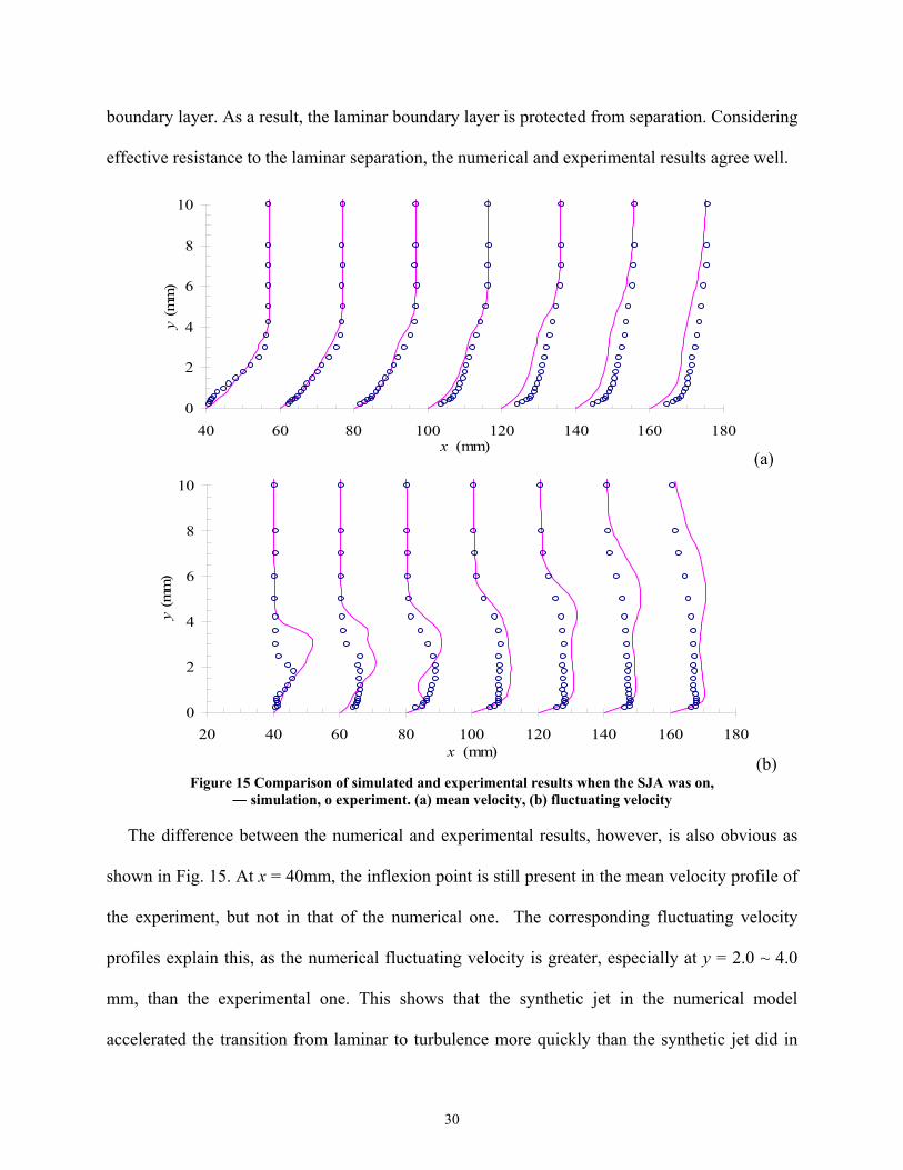
boundary layer. As a result, the laminar boundary layer is protected from separation. Considering
effective resistance to the laminar separation, the numerical and experimental results agree well.
0
2
4
6
8
10
40 60 80 100 120 140 160 180x (mm)
y (m
m)
(a)
0
2
4
6
8
10
20 40 60 80 100 120 140 160 180x (mm)
y (m
m)
(b) Figure 15 Comparison of simulated and experimental results when the SJA was on,
― simulation, o experiment. (a) mean velocity, (b) fluctuating velocity
The difference between the numerical and experimental results, however, is also obvious as
shown in Fig. 15. At x = 40mm, the inflexion point is still present in the mean velocity profile of
the experiment, but not in that of the numerical one. The corresponding fluctuating velocity
profiles explain this, as the numerical fluctuating velocity is greater, especially at y = 2.0 ~ 4.0
mm, than the experimental one. This shows that the synthetic jet in the numerical model
accelerated the transition from laminar to turbulence more quickly than the synthetic jet did in
30

the experiment. The differences between the numerical and experimental results of both mean
and fluctuating velocity profiles are increasing downstream. At the positions close to the wall, y
< 1.0mm, the numerical fluctuating velocity agrees relatively well with the experimental one,
although the differences between the numerical and experimental results of mean velocity
profiles at x = 100~160 mm are noticeable. As we experienced, the baseline flow numerically
simulated is very sensitive to the disturbance triggered by the SJA. The major difference between
the numerical and experimental results is shown by the fluctuating velocity profiles in the upper
region of the boundary layer. Starting from x = 120 mm, as shown in Fig. 15(b), an ‘overhang’
on the fluctuating velocity profile is growing and moving towards the edge of the boundary layer
downstream. This ‘overhang’ may be due to the energy accumulation in the simulation. Further
increasing the width of the computational domain and adding a buffer box at the outlet end of the
computational domain may reduce the ‘overhang’.
Figure 16 shows the comparison of boundary layer thickness for the results shown in Fig. 15.
As shown in Figure 15, the numerical and experimental mean velocity profiles agree better in the
region from x = 40mm to x = 80mm than that in the rest of the region. However, the comparison
of the boundary layer thickness in Figure 16 shows more difference between the numerical and
experimental results in the region from x = 40mm to x = 80mm than that in the rest of the
region. In the region from x = 100mm and x = 160 mm, the numerical boundary layer thickness
agrees well with the experimental one, while the comparison in the same region in Figure 15
shows less agreed results between the simulation and the experiment.
As described previously, Blasius velocity profile was assumed at the inlet of the
computational domain with an adjusted freestream velocity. Instead of simulating the physical
cycle in the actuator, a function of the jet velocity at the center of the exit of the SJA was
31

specified. On the other hand, as we have experienced, the flow simulated was very sensitive to
the disturbance triggered by the synthetic jet. The width of the computational domain and the
grid ratio may also require further improvement when more computational resources are
provided. Therefore, the assumptions made in the initial and boundary conditions and some of
the numerical methods adopted could all contribute to the errors in the numerical simulation.
0
2
4
6
8
10
12
0 20 40 60 80 100 120 140 160 180x (mm)
δ (m
m)
Jet on simulationJet on experiment
Figure 16 Comparison of numerical and experimental results of boundary layer thickness
along the streamwise centerline
In the wind tunnel experiment, it was noticed that the fluctuating velocity with the SJA
operating at a forcing frequency of 100 Hz and forcing amplitude of ±7.5V was smaller than that
without the synthetic jet at x = 160 mm [[9]]. This has led to an idea of enabling the SJA to play
dual roles in enhancing as well as reducing the turbulence to meet various control objectives [9].
Figure 17 compares the fluctuating velocity profiles without the jet to that with the jet at a
forcing frequency of 100 Hz for both experiment and simulation, at x = 160mm. It shows that the
numerically simulated fluctuating velocity with the jet on is also smaller than that without the jet.
This observation from the numerical simulation is consistent with that from the experiment.
32

0.1
1
10
0 0.5 1 1u ' (m/s)
y (m
m)
.5
Experiment with jetExperiment without JetLES with jetLES without jet
Figure 17 Comparison of fluctuating velocity profiles at x = 160mm
8. Interaction between the synthetic jet and the baseline flow
In the wind tunnel experiment, the traverse of the hotwire probe was restricted to streamwise
and normal directions. The experimental data only provided information of the streamwise
velocity measured at a certain number of (x, y) positions along the streamwise centrerline. To
extend our knowledge about the interaction between the synthetic jet and the baseline flow, the
verified numerical model was used.
Figure 18 shows the iso-surfaces of the instantaneous vorticity (a) and the averaged positions
with zero streamwise velocity uavg=0 (b), projected on x-z plane. The instantaneous vorticity of
5600 in Fig. 18(a) was chosen because it was a new vorticity value introduced by the synthetic
jet. Next to the side walls of the computational domain, the behaviour of the flow with the
synthetic jet is similar to that without the synthetic jet, as the flows in both cases break down in
thin streaks around x =100~120mm. (Note that representation of the instantaneous vorticity next
to the side walls may be biased due to the coarser grids). The vortices introduced by the synthetic
33

jet propagate in both streamwise and spanwise directions. However, development of the vorticity
introduced by the synthetic jet remains in the region symmetric about the streamwise centreline
and does not reach the sidewalls of the computational domain. The limited region of this
vorticity development may indicate that to make a SJA effective in both streamwise and
spanwise directions, certain distance between the SJA and the separation bubble is required.
(a) (b)
Figure 18 Top view of the iso-surface of instantaneous vorticity = 5600 (a) and the iso-surface of time-averaged streamwise velocity = 0 (b)
The vorticity concentrated on both sides of the streamwise centreline is further confirmed by
the iso-surface of the averaged positions with uavg = 0, in Fig. 18(b). As shown by the region with
uavg = 0 removed in Fig. 18(b), the laminar separation originally in the baseline flow is
successfully resisted by the synthetic jet. Although the bubble is not entirely removed, the
laminar separation region symmetric about the streamwise centreline has disappeared. The
minimum width of the eliminated separation bubble is about 16mm as measured at x = 90mm,
equivalent to 32 times the jet orifice diameter. Such information should be necessary for
determining the distance between two SJAs in spanwise direction.
The developed model will be applied to help us understand the physics involved in the
experiments. For example, the experimental results showed that the effect of the forcing
frequency on the effect of flow control was more significant than that of the forcing amplitude
34

[8,9]. The numerical simulation may provide more detailed information for us to understand
why. In Figure 19 are two sample results of the simulation, the spanwise vortices in the x-y plane
at z = 0 in (a) and the streamwise vortices which are a pair of vortices on the y-z plane at x = 17
mm. The spanwise vortices at different z positions and the streamwise vortices at different x
positions will be used to analyze the physics associated with the synthetic jets.
(a) x (m)
y (mm)
(b)
Figure 19 a) Spanwise vortices at z = 0, b) Streamwise vortices at x = 17 mm, Forcing frequency = 100 Hz
9. Conclusion
A numerical model of a baseline flow was prepared for investigating the SJA in flow
separation control. It simulates the boundary layer flow field enclosing a ‘short’ laminar
separation bubble caused by adverse pressure gradient. A commercial code was used to solve the
governing equations. The computational domain was three-dimensional and covered the exit of
the SJA. LES was employed to achieve the optimal balance between the computational resources
35

and the accuracy of the numerical modelling. Dynamic Smagorinsky model was used for the
sub-grid scale stress (SGS) terms. The initial and boundary conditions were defined using or
referring to our wind tunnel experiments.
The simulated separation bubble was visualized in various ways to identify the laminar-short
separation bubble. The averaged position with uavg=0 in the inflectional velocity profile was used
to identify the edge of the bubble, including the separation point and the reattachment point. The
iso-surface of vorticity was used to show the quick transition from laminar to turbulence,
characterised in a ‘short’ laminar separation bubble and the mixing of the flow after the
transition. The exponential variation of the maximum fluctuating velocity along the streamwise
direction indicated the linear instability. The influence of the number of time steps was
investigated.
The model for the baseline flow was verified by comparing the numerical and experimental
results including the mean and fluctuating velocity profiles at seven stations on the streamwise
centerline in the separation zone. The agreement between the simulation and the experiment is
reasonably good. The identified separation bubble and the model verification demonstrated that
LES was reasonably capable for capturing the basic features of a ‘short’ separation bubble,
including the transition from laminar to turbulent. However, we must bear in mind that the
difficulty in simulating the transition from laminar to turbulent is still unavoidable.
Based on a reasonable agreement between the experimental and numerical results in the
separation zone of the baseline flow, a synthetic jet was inserted at a position upstream of the
laminar separation bubble in the LES model for the baseline flow. The simulated mean and
fluctuating velocity profiles with the synthetic jets were compared with the experimental ones at
seven positions on the streamwise centerline. In terms of the actuation of the SJA, the
36
experimental and numerical results agreed well as both showed effective elimination of the
separation bubble when the forcing frequency was 100 Hz and the maximum jet velocity at the
exit of the SJA was 6.0 m/s.
The iso-surface of inflectional points with uavg=0 was used to visualize the separation zone
eliminated by the SJA, and the iso-surface of vorticity was used to help understand the associated
physics. They were used to show the interaction between the synthetic jet and the flow to be
controlled.
As we experienced, the baseline flow was very sensitive to the disturbance triggered by the
SJA. The level of difficulties in simulating the transition from laminar to turbulence and in
handling the diffusion increased when the SJA was switched on. However, numerical simulation
has shown its potential in helping the development of SJAs. The outcomes of numerical
simulations should contribute to shortening the time on realizing the use of SJAs in a real world.
Acknowledgments
Assistance provided by Mr. Peter Brady in CFD is gratefully appreciated.
References
[1] Alam, M. and Sandham, N. D., Direct Numerical Simulation of ‘Short’ Laminar
Separation Bubbles with Turbulent Reattachment, J. Fluid Mech, 2000, Vol. 403, pp.
223-250.
[2] Allan, B. G., Holt, M., and Packard, A., Simulation of a controlled airfoil with jets,
NASA/CR-201750, ICASE Report No. 97-55, October 1977.
[3] Gad-el-Hak, M., Flow Control: Passive, Active and Reactive Flow Management
(section 8.10.2), Cambridge University Press, Cambridge, 2000.
37

[4] Galperin, B. and Orzag, S. A., Eds., Large Eddy Simulation of Complex Engineering
and Geophysical Flows, Cambridge University Press, Cambridge, 1993.
[5] Gaster, M., The Structure and Behaviour of Laminar Separation Bubbles, A.R.C. R&M
Report No. 3595, 1969.
[6] Glezer, A. and Amitay, M., Synthetic jets, Annu. Rev. Fluid Mech., 2002, 34:503-29.
[7] Hatman, A. and Wang, T., A Prediction Model for Separated-Flow Transition, ASME
paper, GT-29-237, ASME Turbo Expo ‘98’, Stockholm, Sweden, 1998.
[8] Hong, G., Effectiveness of micro synthetic jet actuator enhanced by flow instability on
controlling laminar separation caused by adverse pressure gradient, Sensors &
Actuators, Physics A, Vol. 132, Issue 2, pp607-615, 2006.
[9] Hong, G., Lee, C., Ha, Q.P., Mack, A.N.F. and Mallinson, S. G., Effectiveness of
synthetic jets enhanced by instability of Tollmien-Schlichting waves, AIAA paper,
2002-2832, 2002.
[10] Honohan, A. M., Amitay, M. and Glezer, A., Aerodynamic control using synthetic jets,
AIAA paper, 2000-2401, 2000.
[11] Kral, L. D., J.F. Donovan, J. F., Cain, A. B. and Cary, A. W., Numerical simulation of
synthetic jet actuator, AIAA paper 97-1824, 28th AIAA Fluid Dynamics Conference,
Snowmass Village, CO, June 29 – July 2, 1997.
[12] Li, Y. and Ming, X., Control of two dimensional jets using miniature zero mass flux
jets, Chinese Journal of Aeronautics. August 2000, Vol. 13, No. 3, pp. 129-133.
[13] Lilly, D. K., A Proposed Modification of the Germano Subgrid Scale Closure Method,
Physics of Fluids, 1992, Vol 4, pp 633-634.
38

[14] Lockerby, D. A. and Carpenter, P. W. Modeling and design of microjet actuation, AIAA
Journal, February 2004, Vol. 42, No. 2, pp220-227.
[15] Ming, X., Dai, C. and Shi, S., A new phenomenon of acoustic streaming, ACTA
MECHANICA AINICA, August 1991, Vol. 7, No. 3, 193-198.
[16] Mittal, R. and Rampunggoon, P., On the virtual aeroshaping effect of synthetic jets,
Brief Communications, Physics of Fluids, April 2002, Vol. 14, No. 4, pp 1533-1536.
[17] Mittal, R., Rampunggoon, P. and Udaykumar, H. S., Interaction of a synthetic jet with a
flat plate boundary layer, AIAA paper, 2001-2773, 2001.
[18] Na, Y. and Moin, P. Direct Numerical Simulation of a Separated Turbulent Boundary
Layer, J. Fluid Mech, 1998, Vol. 374, pp. 379-405.
[19] Ozawa, T., Hong, G. and Mack, A. N. F., CFD modellng of synthetic jets in a boundary
layer at adverse pressure gradient, Proceedings of 5th Pacific Symposium on Flow
Visualisation and Image Processing (5PSFVIP), Daydream Island, Australia, 27-29th
September 2005.
[20] Parekh, D., Palaniswamy, S. and Goldberg, U., Numerical simulation of separation
control via synthetic jets, AIAA paper, 2002-3167, 2002.
[21] Ravi, B. R., Mittal, R. and Najjar, F. M., Study of three-dimensional synthetic jet flow
fields using direct numerical simulation, 42nd AIAA Aerospace Sciences Meeting and
Exhibit, Reno, NV, 5-8 January, 2004.
[22] Redford, J. A. and Johnson, M. W., Predicting transitional separation bubbles, Proc.
TURBOEXPO 2004, International Gas Turbine Congress, Austria, 14-17 June 2004.
39
[23] Rist, U., Instability and transition mechanisms in laminar separation bubbles,
VKI/RTO-LS Low Reynolds Number Aerodynamics on Aircraft including Applications
in Emergency UAV Technology, Rhoda-Saint-Gense, Belgium, 24-28 November 2003.
[24] Rist, U., On instabilities and transition in laminar separation bubbles, Proc. CEAS
Aerospace Aerodynamics Research Conference, Cambridge, UK, 10-12, June 2002.
[25] Rizzetta, D. P., Visbal, M. R. and Stanek, M. J., Numerical investigation of synthetic jet
flowfields, AIAA paper, 98-2910, 29th AIAA Fluid Dynamics Conference,
Albuquerque, NM, June 15-18, 1998.
[26] Rumsey, C.L., “Successes and challenges for flow control simulations”, AIAA-2008-
4313, 2008.
[27] Sagaut, P., Large Eddy Simulation for Incompressible flow, second edition, Springer,
2004.
[28] Seifert, A., Theofilis, V. and Joslin, R. D., Issues in active flow control: theory,
simulation and experiment, AIAA paper, 2002-3277, 2002.
[29] Smagorinsky, J., General Circulation Experiments with the Primitive Equations, I. The
Basic Experiment, Monthly Weather Review, Vol. 91, 1963, pp 99-96.
[30] Smith, B. L. and Glezer, A., Vectoring and small-scale motions effected in free shear
flows using synthetic jet actuators, AIAA paper, 97-0213, 1997.
[31] Wilson, P. G. and Pauley, L. L., Two-dimensional large eddy simulation of a
transitional separation bubble. Symp. On Separated and Complex Flows, ASME/JSME
Fluid Engineering Conf., 1995.
40

[32] Wissink, J. G. and Rodi, W., DNS of Transition in a Laminar Separation Bubble, In I. P.
Castro and P.E. Hancock, editors, Advances in Turbulence IX, proceedings of the Ninth
European Turbulence Conference, CIMNE, 2002.
41


![Tidal Flow Patterns Near A Coastal Headland...In [34], submerged round jets were classified to turbulent (Re ≈ 3300 – 3500), transitional (Re ≈ 1600 – 1700) and laminar (Re](https://static.fdocuments.in/doc/165x107/60d236773826da03bb00555b/tidal-flow-patterns-near-a-coastal-headland-in-34-submerged-round-jets-were.jpg)