Flow Separation Control Using Synthetic Jets on a Flat Plate

Dissertations and Theses

4-2014

Flow Separation Control Using Synthetic Jets on a Flat Plate Flow Separation Control Using Synthetic Jets on a Flat Plate

Karunakaran Saambavi Embry-Riddle Aeronautical University - Daytona Beach

Follow this and additional works at: https://commons.erau.edu/edt

Part of the Aerospace Engineering Commons

Scholarly Commons Citation Scholarly Commons Citation Saambavi, Karunakaran, "Flow Separation Control Using Synthetic Jets on a Flat Plate" (2014). Dissertations and Theses. 180. https://commons.erau.edu/edt/180

This Thesis - Open Access is brought to you for free and open access by Scholarly Commons. It has been accepted for inclusion in Dissertations and Theses by an authorized administrator of Scholarly Commons. For more information, please contact [email protected].

http://commons.erau.edu/

http://commons.erau.edu/

https://commons.erau.edu/edt

https://commons.erau.edu/edt?utm_source=commons.erau.edu%2Fedt%2F180&utm_medium=PDF&utm_campaign=PDFCoverPages

http://network.bepress.com/hgg/discipline/218?utm_source=commons.erau.edu%2Fedt%2F180&utm_medium=PDF&utm_campaign=PDFCoverPages

https://commons.erau.edu/edt/180?utm_source=commons.erau.edu%2Fedt%2F180&utm_medium=PDF&utm_campaign=PDFCoverPages

mailto:[email protected]

FLOW SEPARATION CONTROL USING SYNTHETIC JETS ON A FLAT PLATE

by

KARUNAKARAN SAAMBAVI

A Thesis Submitted to the College of Engineering, Department of Aerospace Engineering

in Partial Fulfillment of the Requirements for the Degree of

Master of Science in Aerospace Engineering

Embry-Riddle Aeronautical University

Daytona Beach, Florida

April 2014

iii

ACKNOWLEDGEMENTS

I would like to express my sincere thanks to my advisor, Dr. Yechiel Crispin for his

continuous support, suggestions and consistent encouragement. The completion of this

thesis would have been impossible without his guidance.

I would like to express my sincere gratitude to the committee members, Dr. Reda

Mankbadi and Dr. Dongeun Seo. I would also like to thank my friends who had helped

me in the process of this thesis.

I cannot finish without expressing my deepest gratitude to my family and special friends

for their continuous support, love, patience and encouragement during my academic

years.

Karunakaran Saambavi

Embry-Riddle Aeronautical University

April, 2014

iv

ABSTRACT

Researcher: Karunakaran Saambavi

Title: Flow Separation Control Using Synthetic Jets on a Flat Plate

Institution: Embry-Riddle Aeronautical University

Degree: Master of Science in Aerospace Engineering

Year: 2014

The primary goal of this thesis is to assess the effect of synthetic jets on flow separation.

CFD simulation is conducted for laminar flow over a flat plate using the commercial

software ANSYS FLUENT. The oscillating zero mass jet flow is simulated by imposing

a harmonically varying boundary condition on the wall surface.

In this work, the effect of synthetic jets for different angles of attack and different

frequencies ranging from 200 Hz to 800 Hz was assessed. The application of the

synthetic jet actuators is based in their ability to energize the boundary layer, thereby

providing significant increase in the lift coefficient.

The performed numerical simulation investigates the flow at Re = 2×106. The oscillatory

injection takes place at one fourth the length of the chord from the leading edge.

Streamline fields and the pressure contours obtained for different angles of attack are

compared with published data. An increase in the lift coefficient can also be observed due

to the pulsating jet flow.

v

TABLE OF CONTENTS

Thesis Committee Review ii

Acknowledgement iii

Abstract iv

List of Tables viii

List of Figures ix

Chapter

I Introduction 1

Motivation 1

Flow Separation 2

Flow Control 4

Theoretical Background 4

Dissertation Outline 6

II Synthetic Jet Actuators 8

Principles of Operation 8

Applications of Synthetic Jets 9

Literature Review 11

vi

III Fundamental Equations and Computational Methods 17

Fundamental Equations 17

Conservation of Mass 17

Conservation of Momentum 18

CFD: Overview 19

Definition, Benefits and Applications of CFD 20

CFD Process 20

FLUENT/ POINTWISE Description 22

IV Numerical Simulation on a Flat Plate 25

Overview 25

Grid Generation 25

Solution Methodology 30

Boundary Conditions 31

Problem Definition in Fluent 33

Definition of Fluid Properties and Equation of State35

Definition of Operating Conditions 35

vii

Definition of Boundary Conditions 35

Solution Execution and Convergence 35

V Results and Discussions 38

Flow over a Flat Plate 31

Synthetic Jets in Quiescent Flow 51

Interaction of Synthetic Jets with Cross-Flow 53

Effect of Frequency 58

VI Conclusions and Future Work 60

References 61

Appendices 65

A Creating the Mesh in POINTWISE 65

B Setting the Problem in FLUENT 14.5 67

C The User- Defined Function for Transient Velocity 69

viii

LIST OF TABLES

Table 1: Flow separation control techniques 7

Table 2: Nodes and Cells in the mesh 26

Table 3: Spacing and number of points on the connector for simple grid 26

Table 4: Nodes and Cells in the mesh including the flat plate 27

Table 5: Spacing and the number of points on the connector 28

Table 6: Physical properties of the numerical simulation 30

Table 7: Streamwise and Cross- stream velocities for different angles of attack 31

Table 8: Boundary conditions for modeling synthetic jets in quiescent medium 36

Table 9: Monitored equations and convergence criteria 37

Table 10: Coefficient of lift computed for different angles of attack at Re =2 × 106 46

ix

LIST OF FIGURES

Figure 1: Schematic of flow separation 3

Figure 2: Schematic of a synthetic jet actuator (not to scale) 9

Figure 3: Two-dimensional grid distribution and boundary conditions used to simulate

the synthetic jet 27

Figure 4: Two-dimensional grid distribution and boundary conditions used for synthetic

jet flat plate simulations 29

Figure 5: The growth of the separation bubble on the surface of the flat plate for

uncontrolled flow for M∞ = 0.1 and Re=2 ×106 and thin airfoil stall 40

Figure 6: Comparison of flow over a flat plate with (a) experimental and (b)

computational results at an angle of attack 3° 41







Figure 10: Comparison of CL results for a flat plate (M∞ = 0.1 and Re = 2×106) with

numerical simulation obtained by Rosas C.R. on NACA 0012 airfoil (M∞ = 0.3 and Re =

x

1×106) and with experimental data from “Theory of wing sections” by Ira H. A. et al. on

NACA 0006 airfoil (Re = 3×106) 47

Figure 11: Comparison of CD vs. CL between the present case for a flat plate (M∞ = 0.1

and Re = 2×106) and the experimental data obtained from “Theory of Wing Sections” by

Ira H. A. et al. on NACA 0006 airfoil (Re = 3×106) 47

Figure 12: Pressure contour plots for a flow over a flat plate measured in Pascals at Re=

2×106 and M∞ = 0.1 48


2×106 and M∞ = 0.1 49


2×106 and M∞ = 0.1 50

Figure 15: Pressure contour plots for the synthetic jet actuation with f = 700 Hz 52

Figure 16: Velocity vectors colored by static pressure during blowing 53

Figure 17: Effect of oscillatory flow separation control on CL on the flat plate at α = 0°

and α = 5°, M = 0.1, Re = 2×106, f = 800Hz, Vj = 3.4 m/s 55


and α = 15°, M = 0.1, Re = 2×106, f = 800Hz, Vj = 3.4 m/s 56

Figure 19: Effect of oscillatory flow separation control on CL on the flat plate at α = 18°.,

M = 0.1, Re = 2×106, f = 800Hz, Vj = 3.4 m/s 57

xi

Figure 20: CL versus angle of attack for a flat plate. The controlled numerical simulation

has been performed on a NACA 0012 at Re = 1× 106 57

Figure 21: Comparison of CD vs. CL between the present case for a flat plate with and

without synthetic jets (M∞ = 0.1 and Re = 2×106) and the experimental data obtained

from “Theory of Wing Sections” by Ira H. A. et al. on NACA 0006 airfoil (Re = 3×106)

58

Figure 22: Influence of the variation of frequency on CL. Simulations correspond to M∞

= 0.1, α = 10° and Re = 2 × 106 59

Figure 23: Response frequency Versus Input frequency 59

1

CHAPTER 1

INTRODUCTION

Motivation

Flow control is one of the leading areas of research in fluid mechanics. One of the

important applications of flow control is in the aerospace industry, where flow control

techniques increase the performance of the aircraft and reduce drag. Flow control can be

used to delay transition, reduce turbulence, prevent separation, and to modify the flow-

field. It is basically an application- dependent technique. Therefore a particular

application must be carefully evaluated through analytical, experimental or numerical

means to reach desired goal.

Among the many active flow control devices, one of the most widely investigated devices

is the synthetic jet actuator which is also known as the zero-net-mass-flux actuator. The

potential applications of this simple device are thrust vectoring of jets, mixing

enhancement in shear layers, reduction in separated flow regions, heat transfer, drag

reduction in turbulent boundary layers, etc. The most important application among these

has been the reduction of separation in flow regimes e.g. on wings at high angles of

attack. Synthetic jet actuator is a very versatile device because it generates unsteady

forcing which has been proven to be more effective than steady forcing. Also synthetic

jet actuator transfers linear momentum to the flow-field without net mass injection.

Therefore the need to supply fluid for blowing and suction is eliminated. This also

eliminates additional energy supply, complicated piping and reduces the inherent losses

2

present in the conventional active flow control devices. The work presented in this

dissertation mainly focuses on the flow separation control using synthetic jet actuators.

Flow Separation

Flow separation is the detachment or breakaway of the fluid from the solid surface and it

takes the forms of eddies and vortices. Flow separation occurs when the velocity at the

wall is zero or negative and an inflection point exist in the velocity profile. It can also be

caused by an adverse pressure gradient in the direction of the flow or due to a geometric

discontinuity, that is, corners, sharp turns or higher angles of attack representing sharply

decelerating flow where the loss in energy leads to separation. Separation thickens the

rotational flow region adjacent to the surface and increases the velocity component

normal to the surface.

Separation is always associated with some kind of losses such as increase in pressure

drag, loss of lift, stall and pressure recovery losses. Vortex shedding is another

undesirable characteristic of separation which causes vibrations in the structure which

leads to serious failures when the resonance frequency is reached.

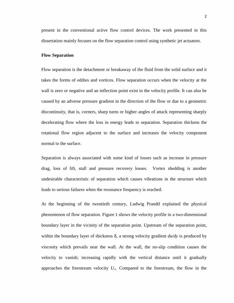
At the beginning of the twentieth century, Ludwig Prandtl explained the physical

phenomenon of flow separation. Figure 1 shows the velocity profile in a two-dimensional

boundary layer in the vicinity of the separation point. Upstream of the separation point,

within the boundary layer of thickness δ, a strong velocity gradient du/dy is produced by

viscosity which prevails near the wall. At the wall, the no-slip condition causes the

velocity to vanish; increasing rapidly with the vertical distance until it gradually

approaches the freestream velocity U∞. Compared to the freestream, the flow in the

3

boundary layer suffers a greater deceleration. This slowing-down process becomes very

noticeable near the surface, that the successive velocity profiles in the streamwise

direction change. The energy associated in the flow close to the surface is small;

therefore the ability of the flow to overcome the adverse pressure gradient becomes

limited. The shear stress opposes the outer-flow field prior to separation because the

velocity gradient near the wall is positive. After separation, the velocity gradient at the

surface is negative. Therefore the separation point occurs at a point where the velocity

gradient vanishes ((du/dy) wall = 0). Downstream of the separation point, the flow adjacent

to the surface reverses in direction so that a circulatory movement in a plane normal to

the surface takes place.

Figure 1: Schematic of flow separation

4

Flow control

The modern use of flow control was initiated by Ludwig Prandtl at the beginning of the

twentieth century, although the idea has been around for centuries. Since then, the

ultimate goal of this extensive research has been to develop techniques to manipulate the

fluid flow to achieve a variety of desired outcomes in industrial applications.

Performance improvement and efficiency maximization in an application involving fluid

flow are the desired goals in achieving flow control. This chapter includes the general

idea of flow control and its advantages, control techniques and a historical perspective.

Theoretical Background

Flow control refers to an attempt of favorably altering the characteristics of the flow-

field. The subject has received significant attention by engineers and scientists since a

desired change in the fluid behavior can be generated by actively or passively controlling

the flow-field. Some of the important advantages of flow control are the benefits it brings

to an industrial application involving fluid flow such as performance improvement, noise

reduction, lift enhancement, prevention of separation, drag reduction, maximization of

efficiency, fuel savings of vehicles, etc.

Prandtl introduced the boundary layer theory and the mechanics of steady separation in

1904, which is now the pioneer of the modern idea of flow control. In his study, he used

active control by applying suction to delay the boundary layer separation from the surface

of a cylinder. No significant advances were made until the 1940s. Laminar flow control

over a wing was the focus shortly before and during the Second World War because the

military required the development of fast and efficient aircrafts, ships and missiles, in

5

which laminar flow control could play a critical role for success. These studies explored

the feasibility of utilizing full-scale boundary layer control over a large aircraft. A

successful example of such studies includes the flight-test program of the X-21, in which

suction was used to delay the transition on a swept wing, which proved the ability to

achieve laminar flow over approximately 75% of the wing surface [1]. Later, in the early

1970s, the oil crisis brought interest in flow control in the transport sector. Studies

including drag reduction for commercial aircraft and other sea/land vehicles were also

investigated to conserve energy. In addition, methods for drag reduction in oil pipelines

and other industrial applications were emphasized by the government agencies and

private corporations. In the 1990s, the flow control studies shifted towards the need to

reduce emissions of greenhouse gases and the construction of super-maneuverable fighter

planes and hypersonic vehicles [2]. Nowadays, the numerical simulations of complex

flows are possible due to the availability of high speed large capacity computers. Many

studies attempt to manipulate coherent structures in transitional and turbulent shear

flows; other studies seek the development of micro-electromechanical system (MEMS)

that can be applied for flow control diagnosis, cooling of electronic components, medical

applications etc.

Flow controls can be active or passive depending on the energy expenditure and the

control loop involved. Passive control methods modify the flow without any auxiliary

power and without a control loop. Some of these techniques include the use of fixed

mechanical vortex generators for separation control; geometric shaping to manipulate the

pressure gradient; and the placement of riblets on the surface for drag reduction. On the

6

other hand, active control methods involve energy and auxiliary power into the flow. The

summary of flow control techniques is given in the

Table 1 below.

Among the active flow control devices, actuators have received a great deal of attention

during the last decade. There are many types of actuators used in active flow control;

some of the most popular include fluidic, thermal, acoustic, piezoelectric,

electrodynamic, electromagnetic and shape-memory alloy actuators. Out of these, the

synthetic jet actuators (also known as zero-net-mass-flux electro-dynamic actuators) will

be the primary focus of this study. Their principles of operation, development and

applications are presented in Chapter 2.

Dissertation Outline

The physical understanding of the behavior of synthetic jet actuators on a flat plate for

active flow control is the main topic of this study. It is accomplished by a computational

approach. The goal of the study is to understand the effect of frequencies and angles of

attack. The studies are performed on a flat plate to evaluate the effectiveness of the

synthetic jet actuator as a flow control device in altering the properties of the boundary

layer. This dissertation is organized into six chapters. An introduction to flow separation

and control is given in the first chapter. Chapter 2 provides a detailed description of the

synthetic jet actuators, their operation and applications and a literature review. The

governing equations and computational methods used are discussed in chapter 3. The

next chapter is about setting up the problem in the CFD tool which is followed by the

7

results and discussions in Chapter 5. Conclusions based on the research performed in this

work are presented in Chapter 6. The final chapter also includes the ideas for future work.

Table 1: Flow separation control techniques

FLOW

SEPARATION

CONTROL

Modification of velocity

profile in the boundary layer

Steady suction

Moving boundaries

Tangential steady blowing

Oscillatory blowing and

suction

Reduction of steepness of

adverse pressure gradient

Surface streamlining

Control of fluid’s viscosity

near the wall

Heat transfer to/from the

fluid

Injection of secondary fluid

with higher/lower viscosity

Cavitation

Chemical reaction

Enhancement of mixing in

shear layer

Vortex generators,

turbulators, etc.

Normal steady blowing

Pulsed jets

Oscillatory blowing and

suction

Additional (active) control

methods

Acoustic excitations

Oscillating flap or wire

Oscillatory surface heating

8

CHAPTER 2

SYNTHETIC JET ACTUATORS

Active flow control using synthetic jets has received people’s attention in recent years. It

deals with suction and blowing into the boundary layer. The addition of energy into the

flow allows the “new” boundary layer to overcome the adverse pressure gradient and

therefore delay separation. The drag coefficient can be significantly decreased by shifting

the transition point in the boundary layer in the downstream direction by using suction.

On the other hand, additional energy is supplied to the fluid particles in the boundary

layer by blowing which enhances the mixing of blowing fluid and oncoming flow within

the boundary layer. The use of oscillatory blowing and suction has been found to be more

effective than just steady blowing or steady suction alone.

The first description of a device similar to “synthetic jet actuator” was given by

K.U.Ingard in 1953 [3]; however, in the recent years there have been significant advances

in the development of “synthetic jet” or “zero-net-mass-flux” actuators which are widely

used for a variety of flow control applications. These actuators require low energy for

operation although they are small in size, low weight and low cost. They can be easily

integrated into the surface of the object as needed e.g. into an airplane wing.

Principles of Operation

The schematic of a synthetic jet actuator is shown in Figure 2. A typical actuator consists

of a cavity open at the top by a small slit through which fluid is free to flow. The flow

9

inside the cavity is driven by a moving surface, either an oscillating piston or a vibrating

diaphragm. The oscillation of the diaphragm produces a fluctuation of the pressure field

in the cavity and at the exit slit, causing it to periodically act as a source and a sink. This

behavior results in a jet originating from the slit. A non-zero momentum is imparted to

the external flow even though there is no net mass injected during a cycle. The slit is the

only communication between the cavity of the actuator and the external flow. Ambient

fluid from the external flow enters the cavity and exits the cavity in a periodic manner.

Upward motion of the diaphragm generates flow which separates at the sharp edges of

the slit and rolls into a pair of vortices generated at the two edges of the slit. These

vortices then move away from the slit at their own induced velocity [4].

Figure 2: Schematic of a synthetic jet actuator (not to scale)

Applications of synthetic jets

Some of the applications of synthetic jets include improving heat transfer, enhancing

mixing, and jet vectoring and controlling a turbulent boundary layer for drag reduction

A. Separation control over Airfoils

The main aim of flow control is to increase lift and decrease drag. This is usually

achieved by controlling the boundary layer flow in order to minimize separation. The

Oscillating diaphragm

10

purpose of this research is to improve aerodynamic performance. The ability to increase

lift at higher angles of attack by preventing separation and stall has important application

in the aerospace industry.

B. Thrust Vectoring

Thrust vectoring is the capability to change the direction of the thrust of an aircraft

engine in a desired direction thereby increasing the maneuverability of the aircraft

without depending completely on the conventional control surfaces. Generally thrust

vectoring is achieved by varying the nozzle geometry; however, the mechanical

complexity of such a variable geometry nozzle results in as much as 30% of the weight of

the engines. One of the most important advantages of thrust vectoring using Active Flow

Control (AFC) is the elimination of the complex movable surfaces that significantly add

weight. Fluidic control (using synthetic jets) of exhaust jet form the engine allows for a

change in the thrust vector for a fixed geometry nozzle. Some other advantages are that

the frequency, amplitude and the phase of the excitation can be controlled; they operate

in harsh thermal environments; they are not susceptible to electromagnetic interference,

they have no moving parts and are easy to integrate into a working device.

C. Forebody Vortex Control (FVC)

The system of vortices that forms and separates from the forebody of an aircraft or a

missile at higher angles of attack affects the aerodynamic loads and moments acting on

the vehicle. These vortex configurations depending on the angle of attack may be

symmetric or asymmetric. The asymmetry may produce strong yawing moments that

cause stability and control problems. Therefore, a method to control the strength and

11

configuration of the separating vortices is of high importance. Forebody Vortex Control

is a technique to manage the loads and moments acting on the vehicle by introducing

controlled perturbations near the forebody nose, where the vortices originate. By flow

control, the asymmetric state of forebody vortices can be made symmetric, thus the side

forces of the vehicle can be eliminated.

D. Control of Flow – Induced Cavity Oscillations

Understanding the flow over open cavities is of great importance for a wide range of

engineering applications including aircraft landing gears, car sunroofs, etc. Self-

sustained oscillations inside the cavity generate intense pressure fluctuations that can lead

to structural damage or failure of critical components; thus suppression of these

oscillations becomes an important flow control problem. In compressible flow, cavity

oscillations arise from a flow-acoustic resonance mechanism involving a feedback

process impinging near the downstream corner of the cavity. This generates acoustic

waves that propagate back upstream and interact with the shear layer to excite further

instabilities. It has been shown that it is possible to suppress these cavity oscillations and

flow induced cavity resonance by employing synthetic jets upstream of the cavity leading

edge.

Literature Review

Some of the earlier active control methods employed the acoustic excitation or a steady

blowing/suction to alter the attached or separated turbulent boundary layer flow on

aerodynamic surfaces. In 1987, Zaman et al. [5] studied the effect of acoustic excitation

on flow separation over airfoils over a large angle-of-attack range. Significant

12

improvement in lift was obtained post stall due to large amplitude acoustic excitations.

Most effective results were produced for frequencies that resulted in large transverse

velocity fluctuations rather than large-amplitude pressure fluctuations. Experiments by

Chang et al. [6] demonstrated the influence of frequency on separation control at post

stall angles of attack. Their results showed that the flow separation was reduced at angles

of attack lower than the stall angle by using small amplitude excitation frequency close to

the shear layer instability frequency. Maximum lift increment (about 50% in lift

coefficient) was found at an angle of attack 22˚. Their data also showed that the effective

forcing frequency reduced separation over a wider range of angles of attack.

The study by Seifert et al. [7] applied a combination of steady and oscillatory blowing to

the surface of a NACA 0015 airfoil in the tangential direction. They proved that larger

increments in lift could be obtained by using a less powerful excitation device if an

oscillatory jet was used instead of a steady jet. A combination of oscillatory blowing with

a small amount of steady blowing proved to be the most efficient method for active flow

control of separation. As an extension of their previous work, Seifert et al. [8] examined

the several parameters including the location of the blowing slot, the steady and the

oscillatory momentum coefficients of the jet, the frequency of the imposed oscillations,

and the shape of the airfoil on reducing separation. They concluded that the most

effective location for the excitation was nearest to the separation location. Since the

earlier experimental work of Seifert, Glezer and Wygnanski among others, the use of

zero-net-mass-flux (ZNMF) has become very prominent for active flow control during

the past decade. These actuators produce oscillatory jets which impart zero net mass into

the flow field suring blowing and suction cycles but impart momentum to the flow.

13

During the past two decades, a number of experiments have been performed to evaluate

the potential of active flow control actuators. James et al. [9] investigated the evolution

of a synthetic round turbulent jet formed by a submerged oscillating diaphragm that is

flush mounted in a flat plate. An isolated synthetic jet is produced by the interactions of a

train of vortices that are typically formed by altering momentary ejection and suction of

fluid across an orifice such that the net mass flux is zero. The time-averaged structure of

the synthetic jet was found similar to convectional round turbulent jet. Smith et al. [10]

also tested synthetic jet actuators at higher frequencies on a 24% thick airfoil in which

flow reattachment was achieved at angles of attack up to 18˚. Their results suggested that

there is a threshold jet momentum below which the excitation had negligible effect on the

flow-field and this threshold jet momentum decreased as the excitation location

approached the separation point.

In 2003, Lee et al. [11] investigated the effects of piezoelectric synthetic jet actuator on

an adverse pressure gradient flow. Hot-wire anemometer was used to measure mean

value of the boundary layer velocity profile. Their results showed that the actuators must

have sufficient velocity output to produce strong enough vortices for effective flow

control. They observed that the excitation frequency played a major role in flow control

rather than the amplitude of oscillation.

Experimental investigations by Smith et al. [12,13] on thrust vectoring using synthetic

jets showed the static pressure near the primary jet flow can be altered by the synthetic

jets adjacent to the primary jet fluid which resulted in the deflection of the primary jet

towards the synthetic jet thus resulting in vectoring of the primary jet. In 2004, in a

workshop held by NASA Langley Research Center, computational methods were

14

compared against the experimental data for three different cases that involved synthetic

jets.

A number of numerical simulations of synthetic jet flow-field have also been reported in

the literature since the late 1990s. In 1997, two-dimensional incompressible calculations

for both laminar and turbulent synthetic jets were reported by Kral et al. [2]. The

harmonic motion of the actuator was simulated with blowing and suction boundary

condition at the orifice exit (the flow within the cavity was not taken into account). The

turbulent solutions were computed using the unsteady Reynolds-averaged Navier-Stokes

(URANS) equations. URANS simulations were conducted on a NACA 0015 airfoil with

a oscillatory jet located at the leading edge in the tangential direction to the surface by

Donovan et al. [14]. The lift coefficients were significantly increased due to the actuator-

like effect. Although regions of separated flow existed the results were in good agreement

with the experimental result of Seifert et al. [8]. Compressible URANS equations were

used by Wu et al. [15] to perform numerical computations on post-stall flow over a

NACA 0012 airfoil. Effect of periodic blowing and suction near the leading edge was

showed in his study though the mesh was not able to capture the details of the jet. An

increase in lift was obtained when the periodic excitation was activated.

Majority of the simulations reported in the literature so far have been performed for two

dimensional configurations. Rizzetta et al. [16] investigated the flow-field of both two-

and three- dimensional high-aspect ratio synthetic jets using direct numerical simulations

(DNS) of unsteady compressible Navier-Stokes equations. In 2001, Mittal et al. [17]

conducted a numerical simulation that included an accurate model of the jet cavity. Their

boundary conditions in the two-dimensional Cartesian grid included moving boundaries.

15

The investigations included synthetic jets in both quiescent and boundary layer flows. In

the quiescent medium the formation of the vortex rings were observed at the orifice exit.

The operational and geometrical parameters of the jet were the key factors that indicated

if the vortices were expelled or ingested back into the cavity. The two-dimensional DNS

simulations conducted by Lee et al. [18] studied the behavior of an array of synthetic jets

pulsing into an initially quiescent medium. It was observed that the jet formation was

highly sensitive to the Reynolds Number.

Two-dimensional incompressible URANS computations were performed by Guo et al.

[19] to simulate the effect on vectoring angle of a single synthetic jet of various

frequencies, amplitudes and angles located at different distances from the primary jet.

These results compared well with the experimental results of Smith et al. [13] when the

effect of actuator cavity was considered.

Interaction of the synthetic jet with the cross-flow is a key area of investigation in active

flow control. Cui et al. [20] performed two-dimensional simulations using the

incompressible Reynolds-averaged Navier Stokes equations. Flow interaction between

the synthetic jet and the external flow for various amplitudes, frequencies and phase

differences was investigated for cases with and without cavity. In 2004, Ravi et al. [21]

employed DNS to study the effect of slot aspect ratio on the formation of three-

dimensional synthetic jets in quiescent and external boundary layer flow. More recently

three- dimensional simulations were reported by Kotapati et al. [22] in 2005 and 2006 for

a test run at NASA Langley Research Center where the actual actuator cavity in the

experiment was approximated as an equivalent rectangular cavity. Their results showed

16

that the URANS calculations are capable of predicting the overall features of the

oscillatory synthetic jet flow-field.

17

CHAPTER 3

FUNDAMENTAL EQUATIONS AND COMPUTATIONAL METHODS

Fundamental Equations

Computational Fluid Dynamics method comprises of solution of Navier Stokes equations

at required points to get the properties of the fluid flow at those points. This technique

exists since the advancement in complex mathematical algorithms in 1930. Simple CFD

problems were solved analytically, but with the increase in fluid flow complexity,

mathematical complexity increases exponentially. With 3D interactive capability and

powerful graphics, use of CFD has gone beyond research and into industry as a design

tool.

The governing equations for computational fluid dynamics (CFD) are based on

conservation of mass, momentum and energy. Fluent uses a finite volume method (FVM)

to solve the governing equations. The FVM involves discretization and integration of the

governing equation over the control volume.

The basic equations for unsteady-state incompressible laminar flow are conservation of

mass and momentum. When heat transfer or compressibility is involved the energy

equation is also required. The governing equations are:

Conservation of Mass

For a chemically non-reacting fluid, the law of conservation of mass states that “the rate

of change in mass inside the control volume must be equal to the decrease of mass out of

18

the control surface”. Thus, the differential form of the continuity equation can be written

as:

Conservation of Momentum

The principle of conservation of momentum is basically an application of Newton’s

second law to an element of fluid. Therefore, when considering a given mass of fluid in a

lagrangian frame of reference, conservation of momentum states “the rate at which the

momentum of the fluid mass in a control volume changes is equal to the net external

force acting on the mass”. The external forces which act on a mass of the fluid may be

classified as body forces (i.e. gravitational or electromagnetic forces) or surface forces

(i.e. pressure and viscous stresses). The equation in the differential form can be written as

follows:

X - Momentum

19

Written out in full:

Y - Momentum

Written out in full:

CFD: Overview

The governing equations of fluid flow have been known for over a century. The Navier-

Stokes equation is a highly non-linear equation whose solution for problems of practical

interest has been possible only after the advent of high-speed large memory computers

only a couple of decades ago. Until 1980s, experimental fluid dynamics was the only real

way of understanding and quantifying the fluid behavior in complex configurations,

sometimes aided by simple analytical/computational models. These experiments are

generally performed on small scale models of the full configurations. In general it is not

feasible to perform experiments on full-scale configurations such as aircrafts,

automobiles, power plants, etc. Furthermore, experimental measurements are quite

expensive and require considerable time to complete and therefore can be performed on a

limited number of models and a limited number of flow configurations. Since 1970s there

20

have been extraordinary advances in the development of both the numerical algorithms

for the solution of the Navier-Stokes equations as well as in computing hardware that it is

now feasible to compute the flow-fields of complete configurations such as an aircraft or

an automobile. A large number of codes such as FLUENT, ANSYS, STARCCM+, CFX,

CFD++ etc. have been developed for a variety of industrial applications. Turbulence

modelling still needs to be investigated as it introduces errors in simulations. However,

substantial progress has been made in the last four decades in the development of

turbulence models to calculate a wide variety of complex flow-fields reasonably

accurately. Computational Fluid Dynamics (CFD) is now considered as an important

branch of fluid dynamics complementing the experimental fluid dynamics.

Definition, Benefits and Applications of CFD

A standard definition of CFD is given in reference which states that it is the science of

determining a numerical solution to the governing equations of fluid flow while

advancing the solution through space or time to obtain a numerical description of the

complete flow-field of interest”. CFD can be applied to solve problems in fluid flow, heat

transfer, mass transfer, acoustics, chemical reactions and related phenomena.

CFD Process

A brief outline of the process for performing a CFD analysis is given in this section.

Several steps are required for modelling fluid flow using CFD. Essentially, there are three

main stages in every simulation process: preprocessing, flow simulation and post-

processing. Preprocessing is the first step in building and preparing a CFD model for the

flow simulation step. This included the problem specification and construction of the

21

computer model via computer-aided design software. Once the computer model is

constructed, a suitable grid or mesh is created in the computational domain. Then the

flow conditions including the material properties of the fluid such as density, viscosity,

thermal conductivity, etc. are specified.

The computational domain should be chosen in such a way that an acceptably accurate

answer is obtained without excessive computations being required. The nature of the

flow-field and the geometry generally provides a guide for a suitable mesh construction

as to its structure (structured, unstructured, zonal or hybrid) and topology (c-, o-, h- or

hybrid). There is also an option to adapt the mesh according to the solution. It can

automatically cluster in regions of higher flow gradients by sensing the solution as it

evolves. The good mesh should display qualities such as orthogonality, lack of skewness

and gradual spacing to obtain accurate solutions.

All the above mentioned steps constitute the preprocessing prior to the second step of

flow simulation, in which the boundary conditions and initial conditions of the problem

must be specified. For the second step, the mesh coordinates the boundary conditions in

the computational domain and the material properties of the fluids are imported into a

flow solver such as FLUENT. The flow solver then executes the solution process for

solving the governing equations of the fluid flow. The governing equations are solved

employing a suitable numerical algorithm which is coded in the flow solver. As the

solution process proceeds, the solution is monitored for convergence implying that there

is little change in the solution from one solution step to the next. Once the solution within

a specified error tolerance is obtained, the post-processing step begins.

22

This step involves the display of converged flow variables in graphical and animated

forms. The post-processing can be conducted using various software like FLUENT,

TECPLOT, etc. Computed flow properties are then compared with the experimental data

(if available) or with the computations of other investigators to validate the solutions. The

simulation is complete at this point although, a sensitivity analysis of the results is

recommended to understand the possible differences in the accuracy of the results with

variations in the mesh size and the other parameters used in the algorithms.

FLUENT / POINTWISE Description

FLUENT is the worlds’ largest provider of commercial CFD software and services.

FLUENT software contains the broad physical modeling capabilities needed to model

flow, turbulence, heat transfer and reactions for industrial applications ranging from air

flow over an aircraft wing to combustion in a furnace, from bubble columns to oil

platforms, from blood flow to semiconductor manufacturing, and from clean room design

to wastewater treatment plants. Special models that give the software the ability to model

in-cylinder combustion, aeroacoustics, turbomachinery and multiphase systems have

served to broaden its reach. FLUENT can be used to solve complex flows ranging from

incompressible (subsonic) to highly compressible (supersonic or hypersonic) including

the transonic regime. FLUENT provides mesh flexibility, including two-dimensional

triangular/quadrilateral meshes and three-dimensional tetrahedral, hexahedral or hybrid

meshes. The grid can also be refined or coarsened based on the flow solution using the

grid adaptation capability. Furthermore, it provides multiple solver options, which can be

modified to improve both the rate of convergence of the simulation and the accuracy of

the computed result. The software code is based on the finite volume method and has a

23

wide range of physical models which allow the user to accurately predict laminar and

turbulent flows, chemical reactions, heat transfer, multiphase flows and other related

phenomena.

Any geometry can be created in CAD software like CATIA or Pro-Engineer and

imported in mesh generating software like POINTWISE, GRIDGEN, GAMBIT etc. For

this research since the geometry is not complicated it is created and meshed in

POINTWISE.

POINTWISE is flexible, robust and reliable software for mesh generation. POINTWISE

provides high mesh quality to obtain converged and accurate CFD solutions especially

for viscous flows over complex geometry.

Mesh generation, also known as grid is the process of forming nodes across the geometry.

Nodes are the points at which the Navier Stokes equations will be solved for the fluid

properties. When these nodes are connected, a mesh is formed and the domain or the

control volume is called discretized.

There are several aspects to be considered for mesh generation. First is the type of the

mesh. There are two main type of mesh: Structured and Unstructured. A structured mesh

has all the nodes arranged such that the cells formed by joining adjacent nodes are

rectangular in shape. This helps in easy reference of each cell making it numerically

simple to deal with. An Unstructured mesh (Figure) has nodes distributed randomly,

hence the mesh cells can be tetrahedral, octahedral and pyramid in shape for 3D mesh

and triangular in shape for 2D mesh. This random arrangement of nodes require a

mapping file to keep the track of the nodes, increasing the file size of unstructured mesh

24

compared to structured mesh. Unstructured mesh is useful for meshing complex and

curved geometries. Since we are dealing with a 2D flat plate structured mesh is used.

Once the model is meshed, the boundary conditions are specified in POINTWISE.

Details about meshing the geometry using POINTWISE is mentioned in Appendix A.

25

CHAPTER 4

NUMERICAL SIMULATION ON A FLAT PLATE:

(Methodology and Solution approach)

Overview

Numerical simulations are a valuable tool, especially when experiments become

complex, expensive and time consuming. The validated computational code can be

employed to conduct a large number of parametric studies for similar configurations

quickly and inexpensively for extensive analysis. Thus, CFD simulations constitute a

crucial part of this study. This chapter describes the methodology and solution approach

used in the numerical simulations. A description of the grid generation procedure is given

first, followed by specifying the boundary conditions. Finally, a detailed step by step set-

up description of a solution using FLUENT is presented.

Grid Generation

The first major step when conducting a CFD analysis is the construction of the geometry

and a suitable mesh. The geometry was both created and meshed using POINTWISE

since the geometry (flat plate) was relatively simple. The synthetic jet was modeled as an

oscillating diaphragm (providing suction and blowing). The first step in setting up the

mesh is the creation of a control area followed by the creation of nodes (points where the

grid lines of the mesh connect) on the edges of the geometry. This process was

accomplished by specifying a gradually increasing or decreasing spacing, which provided

a non-uniform mesh with finer resolution in certain areas of the computational domain

for e.g. near the oscillating diaphragm. Once the nodes were created, actual mesh was

generated. A variety of options for mesh generation are available for mesh generation are

26

available in POINTWISE, including both structured and unstructured elements. Synthetic

jet actuation is initially examined in a quiescent flow which helps verifying the assumed

jet model. Therefore a simple symmetric mesh is generated in POINTWISE. After

several trials, a structured mesh with 242,756 quadrilateral cells was created. The length

of the oscillating diaphragm was 5 cm.

Table 2: Nodes and Cells in the mesh

Table 3: Spacing and number of points on the connector for simple grid

Boundary No. of points Spacing

Oscillating diaphragm 200 0.25

Jet exit 800 0.25 to15.61

Pressure Inlet 300 0.21 to 17.42

27

Figure 3: Two-dimensional grid distribution and boundary conditions used to simulate

the synthetic jet

The flat plate of length 1m and thickness 5 mm was considered for simulations. A

structured mesh was generated in POINTWISE with 167,351 quadrilateral cells. The

oscillating diaphragm was 5 cm in length.

Table 4: Nodes and Cells in the mesh including the flat plate

Pressure Outlet

Pressure

Inlet

Velocity Inlet

(Sinusoidal)

Wall

Pressure

Inlet

28

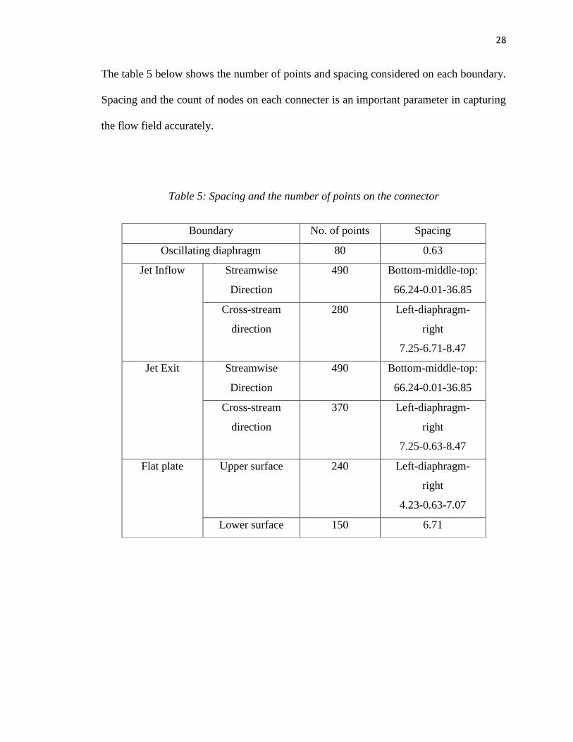
The table 5 below shows the number of points and spacing considered on each boundary.

Spacing and the count of nodes on each connecter is an important parameter in capturing

the flow field accurately.

Table 5: Spacing and the number of points on the connector

Boundary No. of points Spacing

Oscillating diaphragm 80 0.63

Jet Inflow Streamwise

Direction

490 Bottom-middle-top:

66.24-0.01-36.85

Cross-stream

direction

280 Left-diaphragm-

right

7.25-6.71-8.47

Jet Exit Streamwise

Direction

490 Bottom-middle-top:

66.24-0.01-36.85

Cross-stream

direction

370 Left-diaphragm-

right

7.25-0.63-8.47

Flat plate Upper surface 240 Left-diaphragm-

right

4.23-0.63-7.07

Lower surface 150 6.71

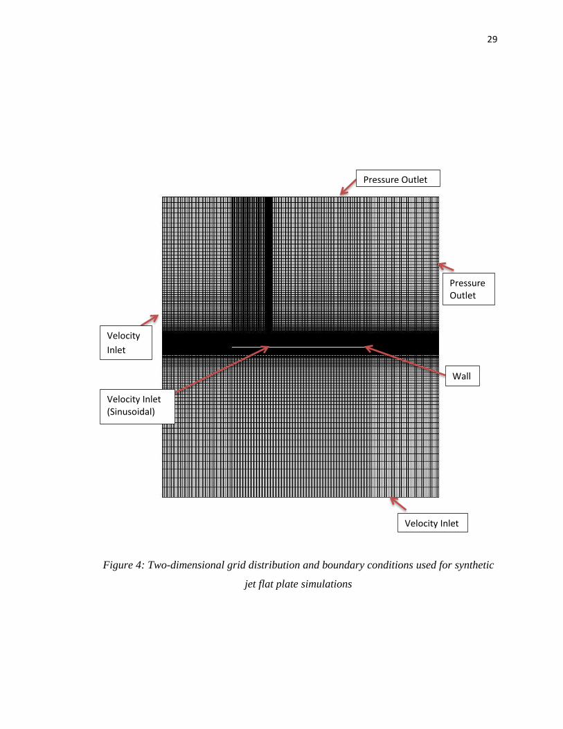
29

Figure 4: Two-dimensional grid distribution and boundary conditions used for synthetic

jet flat plate simulations

Pressure Outlet

Pressure Outlet

Wall

Velocity Inlet

Velocity Inlet (Sinusoidal)

Velocity

Inlet

30

Nomenclature

f: Synthetic jet frequency

x: Streamwise direction tangential to the surface

y: Cross-Stream direction normal to the surface

u: Streamwise velocity

v: Cross- Stream velocity

Vj: Amplitude of the synthetic jet

U∞: Free stream velocity

Solution Methodology

Table 6: Physical properties of the numerical simulation

Pressure 101325 Pa (1 atm)

Temperature 300 K

Speed of sound 340 m/s

Free stream velocity 34 m/s

Kinematic viscosity 1.79(10-5

) kg/ms

Density 1.23 kg/m3

MACH 0.1

Chord 1 m

31

Reynolds Number:

= 2(10

6)

The streamwise velocity (u) and the cross-stream velocity (v) were computed for different

angles of attacks.

Table 7: Streamwise and Cross- stream velocities for different angles of attack

Angle-of-attack u (m/s) v (m/s)

0˚ 34 0

2˚ 33.979 1.187

3˚ 33.953 1.779

4˚ 33.917 2.093

5˚ 33.870 2.963

7˚ 33.747 4.144

9˚ 33.581 5.319

10˚ 33.483 5.904

15˚ 32.841 8.799

18˚ 32.33 10.507

20˚ 31.950 11.629

Boundary Conditions

The correct specification of boundary conditions on the boundaries of the computational

domain is very critical in CFD modeling for obtaining the accurate solutions. Defining

these boundary condition involves boundary location identification (i.e. inlets, outlets,

32

walls, axis, etc.) and flow variables specification. These boundary condition locations for

computational domain are shown in Figure 4. No-slip condition is applied on all the walls

of the flat plate except the diaphragm. In two dimensions, the no-slip condition can be

written as:

and

where x and y describe the coordinates of a point on the fixed boundary at which the

velocity is zero. No-slip condition requires a finer grid near the walls as shown in Figure

4 because of resolution required for boundary layer near the walls.

Other boundary conditions are velocity inlet, pressure outlet, wall and symmetry as

shown in figure. The symmetry condition indicates that the geometry is identical with

respect to a specified boundary. This condition allows the computations to be performed

only for half of the actual model in 2D, resulting in saving a considerable amount of the

computational time. In Figure 3 left half of the model about the line of symmetry is

shown. Outflow conditions were specified at the jet exit (pressure outlet), where a

constant exit pressure of one atmospheric pressure was imposed. The inflow conditions

correspond to the oscillating diaphragm, wherein a sinusoidal velocity inlet boundary

condition, normal to the boundary was specified. This velocity inlet boundary condition

was imposed through a User Defined Function (UDF), which is a function written by the

user in C (programming language) and hooked into the FLUENT solver. The velocity

inlet condition is time periodic simulating the sinusoidal motion of the oscillating

33

diaphragm. Although FLUENT includes a moving wall boundary condition feature,

previous studies by Tang et al. [23] have shown that the use of a velocity inlet condition

instead of a moving boundary condition has significant effect on the jet exit velocity and

resulted in a substantial saving of the computational time. In two dimensions, the velocity

inlet condition at the oscillating diaphragm can be written as:

where Vj is the velocity amplitude of the diaphragm, which was determined such that it

was 10% of the freestream velocity. In equation ω related to the frequency f by the

relation,

Problem definition in FLUENT

Once the grid file was imported into FLUENT, the first step in the solution process

involved checking the mesh for errors. The quality of the grid plays a key role in the

accuracy of the result. Smoothness, skewness and node point distribution are the

attributes associated with the mesh quality. The accuracy of solution of any problem

depends on the density and distribution of the nodes in the mesh. Large truncation errors

may be resulted when there are abrupt changes in the volume between adjacent cells;

therefore the smoothness of the mesh is very important. The cell shapes also have a

significant impact on the accuracy of the result. Skewness is defines as the difference

between the shape of the cell and the shape of an equilateral cell of equivalent volume.

34

Highly skewed cells decrease the accuracy and also destabilize the solution. Another

important parameter that needs to be considered when checking the grid is the cell

volume. The cell volume must be positive; a negative volume is an indication of

improper cell connectivity. Once the grid is verified for its quality, certain modifications

to the geometry can be made (i.e. scaling, translation, rotation, etc.) before proceeding to

the problem definition for initiating the numerical solution process in FLUENT.

The computation of a solution in FLUENT requires specification of a number of

parameters associated with the dimensionality of domain, properties of the fluid, choice

of numerical solution method, the turbulence model, the convergence criteria, whether

the flow is steady or unsteady, etc. The linearization process may take an implicit or

explicit form with respect to the system of dependent variables. In the implicit form, the

unknown value in each cell is computed using a relation that includes both the existing

and unknown values from the neighboring cells. Therefore, each unknown appears in

more than one equation of the system; these equations are therefore solved

simultaneously. In the explicit form the unknown value in each cell is computed using a

relation that includes only the known values, therefore the equation can be solved in a

non-coupled manner one at a time. The dimensionality of the problem needs to be

specified as well; in this case a two-dimensional solution was employed. Due to the

unsteady nature of the flow-field, a time-dependent, first-order accurate implicit time

stepping scheme was employed for the two-dimensional calculations. Under the problem

definition, another specification requires the selection of the flow as inviscid, laminar or

turbulent. Several turbulence models are available for example: the Reynolds stress

model (RSM), k-ω and k-ε. In this study we are dealing only with laminar flow-field.

35

Definition of Fluid Properties and Equation of State

Another input in the problem initialization is the definition of fluid properties. In our

calculations, air was selected as the working fluid from the FLUENT’s database. The

material of the flat plate was considered to be Aluminum. For all calculations, an

incompressible solution method was selected.

Definition of Operating Conditions

Operating conditions include pressure and gravity. Atmospheric pressure was set as the

operating pressure for all test configurations. Gravitational acceleration can also be

specified for any problem. In this case the gravitational effects have been excluded.

Definition of Boundary Conditions

A summary of the boundary conditions for the test configuration for synthetic jets in

quiescent medium is given in Table 8. Once the problem definition, operating conditions,

fluid properties and the boundary conditions are specified, the solution process can be

initiated.

Solution Execution and Convergence

Each test configuration has to be initialized before the code can be executed. This

initialization provides an initial guess for the first iteration of the solution. During this

process the user must specify which part of the computational domain will be provided

with initial conditions. For the synthetic jet actuator flow-field in quiescent medium, the

velocity inlet was selected since the sinusoidal motion was applied at this boundary. Once

36

Table 8: Boundary conditions for modeling synthetic jets in quiescent medium

ZONE TYPE BOUNDARY CONDITION

Oscillating

membrane

Velocity Inlet

Velocity magnitude and direction:

Initial velocity is specified by UDF

x-component: 0

y-component: 1 (unit vector direction)

Flat Plate Wall No-slip condition

Inflow Pressure Inlet Inlet Pressure : 101325 Pa (atmospheric)

Jet Exit Pressure

Outlet

Outlet Pressure : 101325 Pa (atmospheric)

Vertical

Axis

Symmetry Physical geometry and expected flow solution have

mirror symmetry with respect to the vertical axis

the flow field is initialized; the number of iterations must be specified by the user. This

number was selected depending on the frequency of the motion. Each unsteady case was

run for about three seconds before the converged solution was obtained. After three

seconds, the solution became periodic and started to repeat itself in the next cycle. In

some cases more than three seconds were required for the solution to converge.

Several flow properties were monitored and checked for convergence. The employed

convergence criterion required the scaled residuals to decrease to 10-6

for all the

37

governing equations. Also the under relaxation parameters were varied to achieve

convergence. Table shows a list of variables and their respective convergence criterion.

Table 9: Monitored equations and convergence criteria

The user-defined function was written in ‘C’ programming language. A detailed

description of hooking the UDF into FLUENT is explained in Appendix B and C.

The software utilized for the post-processing of the results were ANSYS FLUENT and

TECPLOT. This software was used to generate the scalar and vector fields, animations,

plots of grids and x-y graphs.

Equation Convergence Criteria

Continuity Residual < 10-6

x-momentum Residual < 10-6

y-momentum Residual < 10-6

38

CHAPTER 5

RESULTS AND DISCUSSIONS

Flow over a flat plate

Although the aerodynamic characteristics of airfoil sections are dependent on the shape

of the airfoil and the Reynolds number, the angle-of-attack plays a key role when

computing the lift. A very thin flat plate (5 mm) with a chord length of 1m was

considered for the numerical simulations. Because of the sharp leading edge, flow

separates from the upper surface at the leading edge at an angle of attack as low as 3˚ -5˚

and reattaches further downstream on the surface leaving a separation bubble. As the

angle of attack increases, the reattachment point moves aft and the bubble grows. The

separation bubble covers almost the complete chord and CLmax is reached. This type of

stall is called the thin airfoil stall or long bubble stall. Near the stall, the relationship

between CL and α of the airfoil sections and their stall characteristics are dependent on the

thickness chord ratio, the shape of upper surface near the leading edge, and the Reynolds

Number.

The stream lines and the pressure contours for various angles of attack at Mach 0.1 (U∞ =

34 m/s) is shown below. Also some validation studies have been performed. The

validation is achieved by comparing the results obtained with experimental data and

numerical data obtained from other authors. The quantities that have been compared are

the lift coefficient, drag coefficient and the streamlines. The lift and the drag coefficients

are computed using the equations. [24]

39

Numerical results obtained are compared with NACA 0006 wing section (experimental

data) obtained from “Theory of Wing Sections” by Ira H. Abbott and Albert E. Von

Doenhoff [25]. Also the results have been compared with the numerical results obtained

by Celerino Resendiz Rosas [26] on NACA 0012 airfoil.

The results from the numerical simulation showed that the CLmax is reached for an angle

of attack of 11˚. At an angle of attack of 11˚ the separation bubble covers almost the

complete chord. The streamlines below clearly shows the growth of the separation

bubble.

Angle of Attack 0° Angle of Attack 1° Angle of Attack 2°


40



Figure 5: The growth of the separation bubble on the surface of the flat plate for

uncontrolled flow for M∞ = 0.1 and Re=2 ×106 and thin airfoil stall

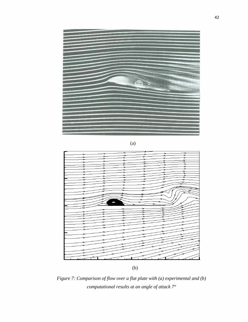
The streamlines obtained from the numerical simulation for a flat plate of 0.5% thickness/

chord ratio has been compared with the flow around a flat plate of 2% thickness/ chord

ratio obtained from “Visualized flow” compiled by the Japanese Society of Mechanical

Engineers [28] as shown in Figure 6 - 9.

41

(a)

(b)


computational results at an angle of attack 3°

42

(a)

(b)



43

(a)

(b)



44

(a)

(b)



45

Coefficient of lift values obtained from the computation was plotted against the angle of

attack to view the pattern as shown in Figure 10. To validate the obtained results they

have been compared with the experimental results of NACA 0006 and numerical results

obtained by Rosas [26] for NACA 0012. Also the Coefficient of Lift (CL) versus the

coefficient of Drag (CD) has been plotted and validated with the experimental results as

shown in Figure 11.

The normal, axial, lift and drag coefficients for an aerodynamic body can be obtained by

integrating the pressure and skin friction coefficients over the body surface from the

leading to the trailing edge. For a two- dimensional body,

∫

∫ (

)

∫ (

) ∫

where

Cp,u – Pressure Coefficient on upper surface

Cp,l – Pressure Coefficient on the lower surface

Cf,u – Friction Coefficient on the upper surface

Cf,l – Friction Coefficient on the lower surface

46

Table 10: Coefficient of lift computed for different angles of attack at Re =2 × 106

Angle of attack (α°) Coefficient of lift (CL)

0 0

1 0.1006

2 0.2381

3 0.3523

4 0.4386

5 0.5483

7 0.7521

9 0.9651

10 1.0982

11 1.1012

12 0.8960

15 0.7023

18 0.6999

47

Figure 10: Comparison of CL results for a flat plate (M∞ = 0.1 and Re = 2×106) with

numerical simulation obtained by Rosas C.R. on NACA 0012 airfoil (M∞ = 0.3 and Re =

1×106) and with experimental data from “Theory of wing sections” by Ira H. A. et al. on

NACA 0006 airfoil (Re = 3×106)

Figure 11: Comparison of CD vs. CL between the present case for a flat plate (M∞ = 0.1

and Re = 2×106) and the experimental data obtained from “Theory of Wing Sections” by

Ira H. A. et al. on NACA 0006 airfoil (Re = 3×106)

0

0.2

0.4

0.6

0.8

1

1.2

1.4

0 5 10 15 20 25 30

CL

Angle of Attack (α°)

Flat plate- Present Solver

NACA 0012 by Rosas C. R.

NACA 0006 experimentaldata

0

0.002

0.004

0.006

0.008

0.01

0.012

0 0.2 0.4 0.6 0.8 1 1.2

CD

CL

Present solver for Flat Plate

Experimental data for NACA0006

48

The pressure contour plots for flow over a flat plate at different angles of attack are

shown in Figures 12 -14. The pressure measured is the gauge pressure in Pa.

Angle of Attack 0° Angle of Attack 1°


Figure 12: Pressure contour plots for a flow over a flat plate measured in Pascals at Re

2×106 and M∞ = 0.1

49




2×106 and M∞ = 0.1

50




2×106 and M∞ = 0.1

51

Synthetic jets in Quiescent flow

Before investigating the interaction of synthetic jets with cross flow, synthetic jet

actuation is examined in a quiescent flow. It helps verifying the assumed jet model and

assessing the formulation of synthetic jets. The flow is assumed to be 2-dimensional,

incompressible and laminar.

Boundary conditions are carefully examined to obtain the accurate result. Initially the

boundary conditions of the model are investigated in quiescent medium and then the

verified boundary conditions are applied to the flow separation simulations.

The boundary layer simulations are performed for a free stream velocity: U∞ = 34m/s.

The frequency of the jet was set to be 700 Hz. (The specific value was chosen so that the

result can be compared with the already obtained value by Kihwan Kim [27])

Synthetic jets in a quiescent flow result from the interactions of a series of vortices that

are created by periodically moving diaphragm. The exiting flow separates at both edges

of the diaphragm and rolls into a pair of vortices during the blowing period as shown in

Figure 15 (a). During the suction period, the flow in the vicinity of the slot comes into the

slot and the created pair of vortices departs from the slot at a self-induced velocity as

shown in Figure 15 (b).

A series of vortex pairs are symmetric with respect to the centerline of the jets. Typically

the moving mechanisms of synthetic jet actuators, e.g. acoustic waves or the motion of

the diaphragm or a piston, induce the pressure drop which alternates periodically across

the exit slot.

52

Although the simulations in this research do not take into account the high-fidelity

modeling for the synthetic jet actuation consisting of cavity, orifice and inner moving

boundary, the result validate that the assumed velocity condition contains the essential

conditions of synthetic jets.

a) At peak blowing

b) At peak suction

Figure 15: Pressure contour plots for the synthetic jet actuation with f = 700 Hz

53

Figure 16: Velocity vectors colored by static pressure during blowing

Figure 16 shows the direction of the velocity vector during blowing. The separation of

the flow into a pair of vortices is showed by the arrows and the length of the arrow

indicates the magnitude of velocity.

Interaction of synthetic jets with Cross-flow

When a synthetic jet interacts with a cross-flow, it creates a complex flow-field structure

in the interaction region, influencing the pressure, velocity and other flow variables. A

continuous deformation is experienced by the jet due to the cross-flow depending on the

momentum causing the streamlines to deflect. As shown in the previous section a pair of

vortex is formed during the blowing stage. Due to the cross-flow, the vortex pair is

deflected to the right. Due to the low velocity of the synthetic jet, the vortices generated

do not penetrate into the free-stream boundary layer. The counter-clockwise vortex

generated at the left is reduced in strength due the clockwise vorticity of the boundary

54

layer. The clockwise vortex at the right gains strength moves downstream along with

cross-flow. The boundary layer is energized due to the high momentum fluid being

entrained into the boundary layer from the blowing part of the synthetic jet. Further away

from the jet this effect is reduced; however, once the flow continuous downstream, it

creates a strong separation bubble immediately downstream of the jet in the vicinity of

the wall. If the mixing of the synthetic jet and cross-flow is strong enough the low

momentum flow close to the wall is energized by the high momentum flow, causing flow

reattachment and thus reducing the or eliminating the separated region.

Important parameters in flow separation control are the excitation frequency, Reynolds

number, the shape of the geometry and the injection point of the synthetic jet. The main

idea in this research was to obtain an increase in the coefficient of lift by introducing the

synthetic jet and to observe the effects of the jet frequency.

Figures 17 to 19 show the lift coefficient, CL, versus the flow time, t. The coefficient of

lift obtained for both controlled and uncontrolled case has been plotted on the same graph

for different angles of attack. Figure 20 shows the mean converged CL, corresponding to

the controlled simulations against the corresponding angle of attack. This figure also

includes the computational results obtained for the uncontrolled flow and the

computational results obtained by Rosas [26]. Figure 20 clearly shows the benefits of

synthetic jet actuation as an increase in the mean lift coefficient of the controlled case

with respect to the uncontrolled case is observed. The result also follows a pattern close

to that obtained by Rosas [26] for a symmetric airfoil. The variation in the result is

possibly due to the geometry. Other probable reason for the discrepancy maybe due to the

laminar model considered.

55


and α = 5°, M = 0.1, Re = 2×106, f = 800Hz, Vj = 3.4 m/s

-0.003

-0.002

-0.001

0

0.001

0.002

0.003

0.004

0 0.5 1 1.5 2 2.5 3

CL

t/(s)

Synthetic jet flow control

Uncontrolled Case

α = 0°

0.54

0.545

0.55

0.555

0.56

0.565

0.57

0.575

0.58

0 0.5 1 1.5 2 2.5 3

CL

t/(s)

Synthetic Jet Flow Control

Uncontrolled Case

α = 5°

56


and α = 15°, M = 0.1, Re = 2×106, f = 800Hz, Vj = 3.4 m/s

1.08

1.1

1.12

1.14

1.16

1.18

1.2

1.22

0 0.5 1 1.5 2 2.5 3

CL

t (s)

Synthetic Jet F low Control

Uncontrolled Flow

α = 10°

-2

-1

0

1

2

3

4

0 0.5 1 1.5 2 2.5 3

CL

t (s)


Uncontrolled Flow

α = 15°

57

Figure 19: Effect of oscillatory flow separation control on CL on the flat plate at α = 18°.,

M = 0.1, Re = 2×106, f = 800Hz, Vj = 3.4 m/s

Figure 20: CL versus angle of attack for a flat plate. The controlled numerical simulation

has been performed on a NACA 0012 at Re = 1× 106

0

0.5

1

1.5

2

2.5

3

0 0.5 1 1.5 2 2.5 3

CL

t (s)

Synthetic JetFlow Control

α = 18°

0

0.2

0.4

0.6

0.8

1

1.2

1.4

0 5 10 15 20 25

CL

Angle of Attack (α°)


Uncontrolled Flow

Controlled numericalsimulation by Rosas

58

Reduction in drag is obtained due to the presence of synthetic jets as observed in Figure

21.

Figure 21: Comparison of CD vs. CL between the present case for a flat plate with and

without synthetic jets (M∞ = 0.1 and Re = 2×106) and the experimental data obtained

from “Theory of Wing Sections” by Ira H. A. et al. on NACA 0006 airfoil (Re = 3×106)

Effect of Frequency

In these simulations, the frequency of the oscillating jet was set to 200, 400, 600 and 800

Hz. The results of these simulations are presented in the figure.

Figure shows that for the two employed frequencies at an angle of attack of 10° the

average lift coefficient remains unchanged (1.1812 and 1.1817 for 400 and 800 Hz

respectively). This may be because the tested frequencies were not large enough.

Frequencies at a higher order of magnitude may produce noticeable effects.

0

0.002

0.004

0.006

0.008

0.01

0.012

0 0.2 0.4 0.6 0.8 1 1.2 1.4

CD

CL

Present solver for flat platewithout synthetic jet

Experimental data for NACA0006

Present solver for flat platewith synthetic jets

59

Figure 22: Influence of the variation of frequency on CL. Simulations corresponds to M∞

= 0.1, α = 10° and Re = 2 × 106

For simulations at Mach number of 0.1 and Re = 2 × 106 the response frequency is much

lower as compared to the input frequency. As the input frequency increases a significant

increase in the response frequency is observed.

Figure 23: Response frequency Versus Input frequency

1.08

1.1

1.12

1.14

1.16

1.18

1.2

1.22

0 0.5 1 1.5 2 2.5 3

CL

t (s)

f = 400 Hz

f = 800 Hz

0

2

4

6

8

10

12

0 200 400 600 800 1000

Response Frequency (Hz)

Input frequency (Hz)

60

CHAPTER 6

CONCLUSIONS AND FUTURE WORK

This chapter summarizes the work presented in this dissertation. Previous chapters have

presented the results of the numerical investigation of a synthetic jet actuator. It allowed

for the identification of critical parameters which influence the performance of the

actuator. The primary idea was to increase the coefficient of lift using the oscillatory jet.

The simulation was conducted on a flat plate for a two-dimensional case. The numerical

tool employed for the simulation was ANSYS FLUENT. The results are validated for

steady simulations over the flat plate. And also agrees with the experimental and

numerical results obtained by various authors. A significant increase in the coefficient of

lift is observed.

The phenomenon of flow separation control by synthetic jets delays separation by

amplifying the disturbances which convect downstream along the flat plate. There is not

only a significant increase in lift but also reduction in drag. Finally, and in the view of the

results obtained, synthetic jet actuator is a good device to control the flow.

This research dealt with flow for over a flat plate for a laminar flow model. The results

can be further improved and developed considering the additional turbulence models and

for airfoils with camber. Also the effect of Reynolds number can be studied.

61

REFERENCES

[1] Jenkins,D.R.et al., “American X-Vehicles: An Inventory X-1 to X-50 Centennial

of Flight Edition”. Monographs in Aerospace History No. 31, SP-2003-4531, June

2003

[2] Kral, L.D., “Active Flow Control Technology”, ASME Fluids Engineering

Division Technical Brief. 1999

[3] Gad-el-Hak, M., Flow Control: Passive, Active and Reactive Flow Management.

Cambridge University Press, 2000.

[4] Auerbach, D., “Experiments on the Trajectory and Circulation of the Starting

Vortex”. J. Fluid MECH Vol. 183, pp. 185-198, 1987.

[5] Zaman, K., et al., “Effect of Acoustic Excitation on the Flow Over a Low Re

Airfoil”, Journal of Fluid Mechanics, Vol. 182, pp. 127-148, 1987.

[6] Chang, R., Hsiao, F. and Shyu, R. “Forcing Level Effects of Internal Acoustic

Excitation on the Improvement of Airfoil Performance”, Journal of Aircraft, Vol.

20, No. 5, pp. 823-829, 1992.

[7] Seifert, A. Bachar, T. Wygnanski, I., Koss, D. Shepshelovich, M., "Oscillatory

Blowing, a Tool To Delay Boundary Layer Separation", AIAA Paper 93-0440 -

presented at the 31st AIAA Aerospace Sciences Meeting, January 1993.

[8] Seifert, A., Darabi, A. and Wygnanski, I., "Delay of Airfoil Stall by Periodic

Excitation", Journal of Aircraft, Vol. 33, No. 4, pp. 691-698, 1996.

[9] James, R.D, Jacobs, J.W, and Gelezer, A., "A Round Turbulent Jet Produced by an

Oscillating Diaphragm", Physics of Fluids, Vol. Issue 9, pp. 2484-2495, September

1996.

62

[10] Smith, D.R., et al., "Modification of Lifting Body Aerodynamics Using Synthetic

Jet Actuators", AIAA 1998-0209 - presented at the 36' Aerospace Sciences Meeting

and Exhibit, Reno, NV, January 12-15, 1998.

[11] Lee, C, Ha, Q.P., Hong, G. and Mallinson, S., "A Piezoelectrically Actuated Micro

Synthetic Jet for Active Flow Control", Sensors and Actuators A, Vol. 108, No.

l,pp. 168-174, November 2003.

[12] Smith, B. L., and Glezer, A., "Vectoring and Small-Scale Motions Effected in Free

Shear Flows Using Synthetic Jet Actuators", AIAA Paper 97-0213, January 1997.

[13] Smith, B.L, Trautman, M.A., and Glezer, A., "Controlled Interactions of Adjacent

Synthetic Jets", AIAA-1999-669 - presented at the 37' Aerospace Sciences Meeting


[14] Donovan, J.F., Krai, L.D. and Cary, A.W., "Active Flow Control Applied to an

Airfoil", AIAA Paper 98-0210 -presented at the 36' Aerospace Sciences Meeting


[15] Wu, J., Lu, X., Denny, A., Fan, M. and Wu, J., "Post-stall Flow Control on an

Airfoil by Local Unsteady Forcing", Journal of Fluid Mechanics, Vol. 371, Issue

01, pp. 21-58, 1998.

[16] Rizzetta, D.P., Visbal, M.R. and Stanek, M.J., "Numerical Investigation of

Synthetic-Jet Flowfields". AIAA Journal, Vol. 37, No. 8, pp. 919-927, 1999.

[17] Mittal, R., Rampunggoon, R. and Udaykumar, H.S., "Interaction of a Synthetic Jet

with a Flat Plate Boundary Layer", AIAA Paper 2001-2773, 2001.

[18] Lee, C. Y. and Goldstein, D. B., "Two-dimensional Synthetic Jet Simulation",

AIAA Journal Vol. 40, No. 3, pp. 510-516, March 2002.

63

[19] Guo, D., Krai, L.D. and Cary, A.W, "Numerical Simulation of the Interaction of

Adjacent Synthetic Jet Actuators", AIAA-2000-2565 - presented at the Fluids 2000

Conference and Exhibit, Denver, CO, June 19-22, 2000.

[20] Cui, J., Agarwal, R.K., and Cary, A.W., "Numerical Simulation of the Interaction

of a Synthetic Jet with a Turbulent Boundary Layer", AIAA-2003-3458 - presented

at the 33rd AIAA Fluid Dynamics Conference and Exhibit, Orlando, Florida, June

23-26, 2003.

[21] Ravi, B. R., Mittal, R. & Najjar, F. M. "Study of Three-dimensional Synthetic Jet

Flowfields Using Direct Numerical Simulations", AIAA Paper 2004-0091

presented at the 42nd AIAA Aerospace Sciences Meeting and Exhibit, Reno, NV,

January 5-8, 2004.

[22] R. Kotapati and R. Mittal, "Time-Accurate Three-Dimensional Simulations of

Synthetic Jets in Quiescent Air", AIAA-2005-103 -presented at the 43rd AIAA

Aerospace Sciences Meeting and Exhibit, Reno, NV, January 10-13, 2005.

[23] Tang, H. and Zhong, S., "An Incompressible Flow Model of Synthetic Jet

Actuators," AIAA Journal, Vol. 44, No. 4, pp. 908-912, 2006.

[24] John D. Anderson, Jr., “Fundamentals of Aerodynamics”, Mc Graw Hill, Third

edition, 2001.

[25] Ira H. Abbott and Albert E. Von Doenhoff, “Theory of Wing Sections”, Dover,

1959

[26] Celerino Resendiz Rosas, “Numerical Simulation of Flow Separation Control by

Oscillatory Fluid Injection”. Ph. D Thesis, Texas A&M University, May 2005

64

[27] Kihwan Kim, “Feedback Control of Flow Separation Using Synthetic Jets”. Ph.D

Thesis, Texas A&M University, December 2005

[28] “Visualized Flow”, Compiled by The Japan Society of Mechanical Engineers.

65

APPENDIX A

Creating the mesh in POINTWISE

1. Creating the geometry

Create > Draw Curves > line

A new dialog box appears in which connector is selected as the entity type.

2. The number of points and the spacing is adjusted according to the need of the

computation (more points required near the oscillating diaphragm to capture the

vortices)

3. Creating domains

Grid > Set Type > Structured

Create > Assemble Special > domain

The connectors are selected to form a completed loop.

When all the domains are created click OK

4. Initializing the grid

Grid > Solve > Initialize

5. Selecting the solver type and dimension

CAE > Select Solver, select ANSYS FLUENT

CAE > Set dimension, 2-D

6. Creating Boundary Conditions

CAE > Set Boundary Conditions

Create new boundaries named Flat Plate, Diaphragm, Velocity Inlet X & Y,

Pressure Outlet X & Y and select appropriate boundary in the geometry to

assign the boundary condition.

66

7. Exporting the generated mesh

Select the Domain.

File > Export > CAE

Save the file as .cas to work in FLUENT 14.5, save the file as .pw file for

future modifications.

67

APPENDIX B

Setting the problem in FLUENT 14.5

This setup is for the flow over a flat plate with a oscillating diaphragm on the upper

surface of the flat plate.

1. Start FLUENT 14.5 and import the .cas file. A dialog box appears in which select the

following

Dimension >2D

Check double precision

Check display mesh after reading

Click OK

File > Read > Case

2. Initial solution setup steps are followed as follows:

The mesh is scaled from mm to m.

Then mesh check is performed the quality is checked. Orthogonal quality

ranges from 0 to1 where values close to 0 correspond to low quality.

3. Then the pressure based solver is selected for a transient flow.

4. The user defined function (UDF) is interpreted for the sinusoidal velocity of the

diaphragm.

Define > Function > Interpret

Browse > Interpret > Close

5. Viscous laminar model is chosen for the simulation

68

6. The next tab allows us to choose the material being used. Air is selected for which the

properties are already defined in the FLUENT database.

7. Then boundary conditions are verified (table []) and the zone which contains the

oscillating diaphragm is chosen to modify the velocity specification method to

components so that the UDF can be interpreted.

8. Reference values are computed form the velocity inlet boundary.

9. Standard pressure and first order upwind momentum spatial discretization is chosen

as solution methods.

10. The under- Relaxation factors are set at default values.

11. Depending on the requirement of the particular case the monitors are created. The

convergence criteria for the residuals were set at 106 for both continuity and

momentum equations.

12. Then the solution is initialized.

13. The time step size (s) and the number of time steps are chosen depending on the

frequency of the periodic motion. Then the solution is calculated.

14. Once the converged solutions are obtained post processor results were analyzed in

TECPLOT.

15. The pressure, vorticity and velocity contour plots were obtained and the velocity

stream lines were plotted.

69

APPENDIX C

The User Defined function for transient velocity

/**********************************************************************

inlet_velocity_profile.c

UDF for specifying a transient velocity profile boundary condition

***********************************************************************/

#include "udf.h"

DEFINE_PROFILE(inlet_velocity, thread, position)

{

face_t f;

real t = CURRENT_TIME;

begin_f_loop(f, thread)

{

F_PROFILE(f, thread, position) = Vj*sin(ω*t);

}

end_f_loop(f, thread)

Flow Separation Control Using Synthetic Jets on a Flat Plate

Documents

Transcript of Flow Separation Control Using Synthetic Jets on a Flat Plate