

Lecture20: Graph IV Bohyung Han CSE, POSTECH [email protected] CSED233: Data Structures (2014F)
33
-
Upload
gwendoline-hamilton -
Category
Documents
-
view
219 -
download
2
Transcript of Lecture20: Graph IV Bohyung Han CSE, POSTECH [email protected] CSED233: Data Structures (2014F)

2 CSED233: Data Structuresby Prof. Bohyung Han, Fall 2014
Weighted Graph
• Properties Each edge has an associated numerical value, weight of the edge Edge weights may represent, distances, costs, etc.
• Example: In a flight route graph, the weight of an edge represents the distance
in miles between the endpoint airports
ORD
PVD
MIA
DFW
SFO
LAX
LGA
HNL
849
802
13871743
1843
1099
1120
1233337
2555
142

3 CSED233: Data Structuresby Prof. Bohyung Han, Fall 2014
Shortest Paths
• What is the shortest path? A path of minimum total weight between two vertices Length of a path is the sum of the weights of its edges.
• Applications Internet packet routing Flight reservations Driving directions
ORD
PVD
MIA
DFW
SFO
LAX
LGA
HNL
849
802
13871743
1843
1099
1120
1233337
2555
142

4 CSED233: Data Structuresby Prof. Bohyung Han, Fall 2014
Shortest Paths
• Properties A subpath of a shortest path is itself a shortest path There is a tree of shortest paths from a start vertex to all the other
vertices
• Example: Tree of shortest paths from Providence
ORD
PVD
MIA
DFW
SFO
LAX
LGA
HNL
849
802
13871743
1843
1099
1120
1233337
2555
142

5 CSED233: Data Structuresby Prof. Bohyung Han, Fall 2014
Dijkstra’s Algorithm
• Problem definition Find the shortest path from a starting vertex to all other vertices.
• Assumptions: The graph is connected. The edges are undirected. The edge weights are nonnegative.
• Methodology We grow a “cloud” of vertices, beginning with a starting vertex and
eventually covering all the vertices. Solve for vertices close to starting vertex: Neighbors are easy to
determine. Add an edge one by one
• Find the path to each vertex one by one• Iteratively expand the set of nodes where the shortest path is known.

6 CSED233: Data Structuresby Prof. Bohyung Han, Fall 2014
Dijkstra’s Algorithm
• Procedure sketch We starts with a vertex . We store each vertex with a label representing the distance of from s
in the subgraph consisting of the cloud and its adjacent vertices.
At each step• We add to the cloud the vertex outside the cloud with the smallest
distance label, .• We update the labels of the vertices adjacent to .
• Avoid adding edges where “future path” may be better Cost is positive and additive. Path cost can not go down later.
7 CSED233: Data Structuresby Prof. Bohyung Han, Fall 2014
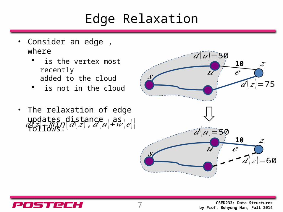
Edge Relaxation
• Consider an edge , where is the vertex most recently
added to the cloud is not in the cloud
• The relaxation of edge updates distance as follows:
10
𝑠
𝑑 (𝑧 )←min {𝑑 (𝑧 ) ,𝑑 (𝑢 )+𝑤 (𝑒 ) }
𝑢
𝑑 (𝑢)=50
𝑑 (𝑧 )=75
𝑧𝑒
10
𝑠 𝑢
𝑑 (𝑢)=50
𝑒𝑑 (𝑧 )=60
𝑧

8 CSED233: Data Structuresby Prof. Bohyung Han, Fall 2014
CB
A
E
D
F
48
7 1
2 5
2
3 9
Example
CB
A
E
D
F
0
428
∞ ∞
48
7 1
2 5
2
3 9
0
328
5 11
CB
A
E
D
F
0
328
5 8
48
7 1
2 5
2
3 9
CB
A
E
D
F
0
327
5 8
48
7 1
2 5
2
3 9

9 CSED233: Data Structuresby Prof. Bohyung Han, Fall 2014
Example
CB
A
E
D
F
0
327
5 8
48
7 1
2 5
2
3 9
CB
A
E
D
F
0
327
5 8
48
7 1
2 5
2
3 9

10 CSED233: Data Structuresby Prof. Bohyung Han, Fall 2014
Dijkstra’s Algorithm
• Heap-based priority queue Stores the vertices outside
the cloud Key: distance Value: vertex replaceKey(l,k):
changes the key of entry l
• We store two labels with each vertex: Distance Entry in priority queue
Algorithm DijkstraDistances(G, s) Q new heap-based priority queue for all v G.vertices() if v = s v.setDistance(0) else v.setDistance() l Q.insert(v.getDistance(), v) v.setEntry(l) while Q.empty() l Q.removeMin()
u l.getValue()for all e u.incidentEdges() // relax e z e.opposite(u) r u.getDistance() + e.weight() if r < z.getDistance() z.setDistance(r) Q.replaceKey(z.getEntry(), r)

11 CSED233: Data Structuresby Prof. Bohyung Han, Fall 2014
Analysis of Dijkstra’s Algorithm
• Graph and label operations Method incidentEdges() is called once for each vertex. We set/get the distance and locator labels of vertex times. Setting/getting a label takes time.
• Priority queue operations Each vertex is inserted once into and removed once from the priority
queue, where each insertion or removal takes time. The key of a vertex in the priority queue is modified at most
times, where each key change takes time.
• Time complexity with the adjacency list structure Recall that
12 CSED233: Data Structuresby Prof. Bohyung Han, Fall 2014
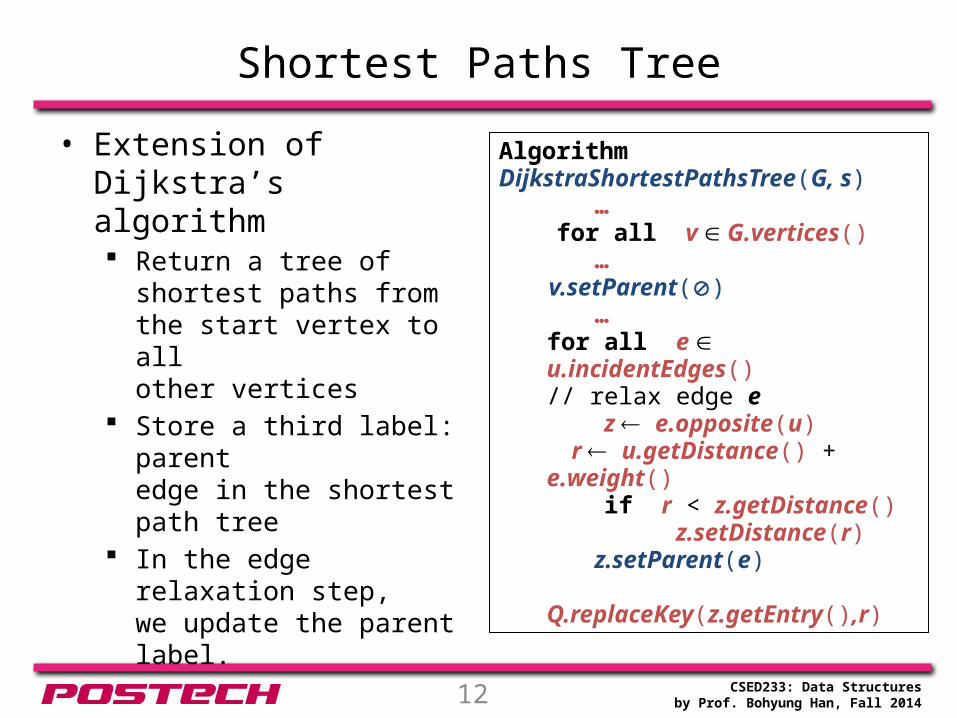
Shortest Paths Tree
• Extension of Dijkstra’s algorithm Return a tree of shortest paths
from the start vertex to all other vertices
Store a third label: parent edge in the shortest path tree
In the edge relaxation step,we update the parent label.
Algorithm DijkstraShortestPathsTree(G, s)…
for all v G.vertices()…
v.setParent()…
for all e u.incidentEdges()// relax edge e z e.opposite(u) r u.getDistance() + e.weight() if r < z.getDistance() z.setDistance(r)
z.setParent(e)
Q.replaceKey(z.getEntry(),r)

13 CSED233: Data Structuresby Prof. Bohyung Han, Fall 2014
Why Dijkstra’s Algorithm Work
• Greedy algorithm: It adds vertices by increasing distance. Suppose it didn’t find all shortest distances. Let be the first wrong
vertex the algorithm processed. When the previous node, , on the true shortest path was considered,
its distance was correct But the edge was relaxed at that time! Thus, so long as ,
’s distance cannot be wrong. That is, there is no wrong vertex.
CB
A
E
D
F
0
327
5 8
48
7 1
2 5
2
3 9
14 CSED233: Data Structuresby Prof. Bohyung Han, Fall 2014
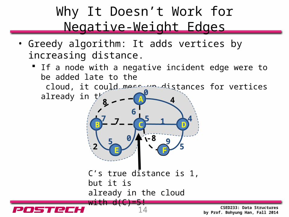
Why It Doesn’t Work for Negative-Weight Edges
• Greedy algorithm: It adds vertices by increasing distance. If a node with a negative incident edge were to be added late to the
cloud, it could mess up distances for vertices already in the cloud.
CB
A
E
D
F
0
457
5 9
48
7 1
2 5
6
0 -8
C’s true distance is 1, but it is already in the cloud with d(C)=5!

15 CSED233: Data Structuresby Prof. Bohyung Han, Fall 2014
Bellman-Ford Algorithm
• Characteristics Works even with negative
weight edges Must assume directed edges:
otherwise we would have negative-weight cycles
• Procedure Iteration finds all shortest
paths that use edges.
• Running time: • Extension
Detecting a negative-weight cycle if it exists
Algorithm BellmanFord(G, s) for all v G.vertices() if v = s v.setDistance(0) else v.setDistance() for i 1 to n - 1 do for each e G.edges() // relax edge e
u e.origin() z e.opposite(u) r u.getDistance() + e.weight() if r < z.getDistance() z.setDistance(r)

16 CSED233: Data Structuresby Prof. Bohyung Han, Fall 2014
Bellman-Ford Example
8
-2
0
48
7 1
-2 5
-2
3 9
-2
0
4
48
7 1
-2 53 9
-2
-28
0
4
48
7 1
-2 53 9
6
-2
-28
0
4
9
48
7 1
-2 53 9
6

17 CSED233: Data Structuresby Prof. Bohyung Han, Fall 2014
Bellman-Ford Example
-25
0
1
-1
4
48
7 1
-2 5
-2
3 9
-2
-25
0
-1
9
48
7 1
-2 53 9
1

18 CSED233: Data Structuresby Prof. Bohyung Han, Fall 2014
Directed Acyclic Graph (DAG)
• Definition A digraph that has no directed cycles Digraph (directed graph): a graph whose
edges are all directed
• Properties Each edge goes in one direction. Edge goes from to , but not to . If is simple, If we keep in edges and out- edges in separate adjacency lists, we can ‐
perform listing of incoming edges and outgoing edges in time proportional to their size

19 CSED233: Data Structuresby Prof. Bohyung Han, Fall 2014
DAG Applications
Procedure of a particular task
Hasse diagram

20 CSED233: Data Structuresby Prof. Bohyung Han, Fall 2014
Topological Sort
• Topological ordering in a DAG Numbering vertices such that, for every edge ,
we have .
Algorithm TopologicalSort(G) H G // Temporary copy of G n G.numVertices() while H is not empty do Let v be a vertex with no outgoing edges Label v n n n - 1 Remove v from H
𝑣1
𝑣2
𝑣3
𝑣4 𝑣5

21 CSED233: Data Structuresby Prof. Bohyung Han, Fall 2014
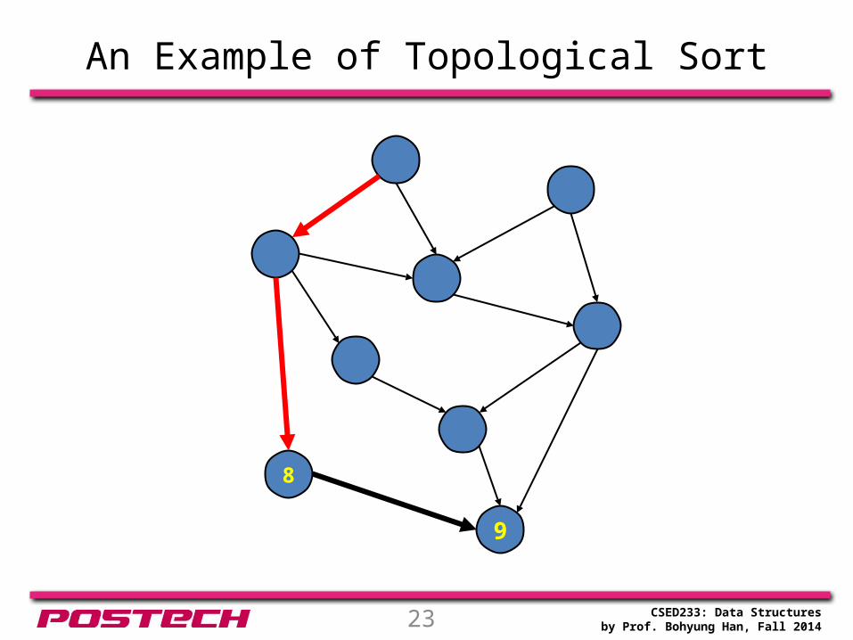
An Example of Topological Sort

22 CSED233: Data Structuresby Prof. Bohyung Han, Fall 2014
An Example of Topological Sort
9
23 CSED233: Data Structuresby Prof. Bohyung Han, Fall 2014
An Example of Topological Sort
9
8
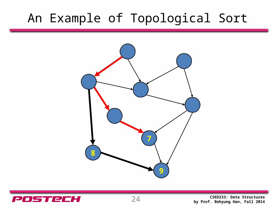
24 CSED233: Data Structuresby Prof. Bohyung Han, Fall 2014
An Example of Topological Sort
7
9
8

25 CSED233: Data Structuresby Prof. Bohyung Han, Fall 2014
An Example of Topological Sort
6
7
9
8

26 CSED233: Data Structuresby Prof. Bohyung Han, Fall 2014
An Example of Topological Sort
56
7
9
8

27 CSED233: Data Structuresby Prof. Bohyung Han, Fall 2014
An Example of Topological Sort
4
56
7
9
8

28 CSED233: Data Structuresby Prof. Bohyung Han, Fall 2014
An Example of Topological Sort
34
56
7
9
8

29 CSED233: Data Structuresby Prof. Bohyung Han, Fall 2014
An Example of Topological Sort
2
34
56
7
9
8

30 CSED233: Data Structuresby Prof. Bohyung Han, Fall 2014
An Example of Topological Sort
2
34
1
56
7
9
8

31 CSED233: Data Structuresby Prof. Bohyung Han, Fall 2014
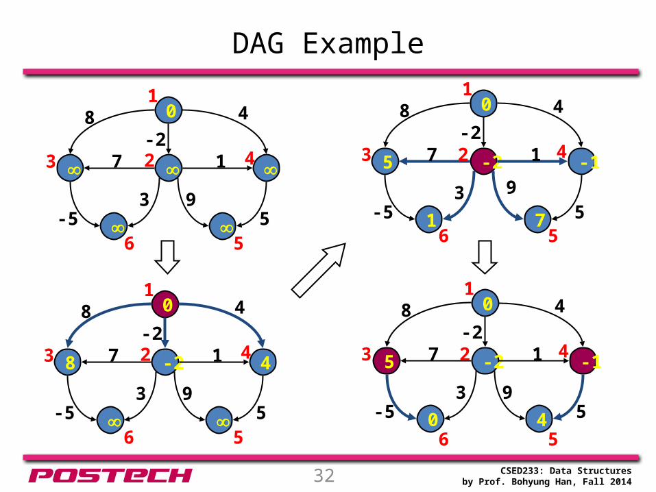
DAG-based Shortest Path Algorithm
• Characteristics Works even with negative
weight edges Doesn’t use any fancy data
structures Uses topological order Is much faster than Dijkstra’s
algorithm Running time:
Algorithm DagDistances(G, s) for all v G.vertices() if v = s v.setDistance(0) else v.setDistance() // Perform a topological sort of the vertices for u 1 to n do // in topological order for each e u.outEdges()
// relax edge e z e.opposite(u) r u.getDistance() + e.weight() if r < z.getDistance() z.setDistance(r)
Why is this faster?
32 CSED233: Data Structuresby Prof. Bohyung Han, Fall 2014
DAG Example
0
48
7 1
-5 5
-2
3 9
1
2 43
6 5
8
-2
-2
0
4
48
7 1
-5 53 9
1
2 43
6 5
-25
0
0
-1
4
48
7 1
-5 5
-2
3 9
1
2 43
-2
-25
0
-1
7
48
7 1
-5 53 9
1
1
2 43
6 5
6 5

33


![Lecture 10: Other Applications of CNNscvlab.postech.ac.kr/~bhhan/class/cse703r_2017f/csed703r_lecture10.pdf · [Aubry14] M. Aubry, D. Maturana, A. Efros, and J. Sivic, Seeing 3D Chairs:](https://static.fdocuments.in/doc/165x107/5be8144a09d3f26f698db4a3/lecture-10-other-applications-of-bhhanclasscse703r2017fcsed703rlecture10pdf.jpg)