Learning Deconvolution Network for Semantic Segmentation

Hyeonwoo Noh Seunghoon Hong Bohyung HanDepartment of Computer Science and Engineering, POSTECH, Korea

{hyeonwoonoh ,maga33,bhhan}@postech.ac.kr

Abstract

We propose a novel semantic segmentation algorithm bylearning a deconvolution network. We learn the networkon top of the convolutional layers adopted from VGG 16-layer net. The deconvolution network is composed of de-convolution and unpooling layers, which identify pixel-wiseclass labels and predict segmentation masks. We apply thetrained network to each proposal in an input image, andconstruct the final semantic segmentation map by combin-ing the results from all proposals in a simple manner. Theproposed algorithm mitigates the limitations of the exist-ing methods based on fully convolutional networks by in-tegrating deep deconvolution network and proposal-wiseprediction; our segmentation method typically identifies de-tailed structures and handles objects in multiple scales nat-urally. Our network demonstrates outstanding performancein PASCAL VOC 2012 dataset, and we achieve the best ac-curacy (72.5%) among the methods trained with no externaldata through ensemble with the fully convolutional network.

1. IntroductionConvolutional neural networks (CNN) have shown ex-

cellent performance in various visual recognition problemssuch as image classification [15, 22, 23], object detec-tion [7, 9], semantic segmentation [6, 18], and action recog-nition [12, 21]. The representation power of CNNs leadsto successful results; a combination of feature descriptorsextracted from CNNs and simple off-the-shelf classifiersworks very well in practice. Encouraged by the successin classification problems, researchers start to apply CNNsto structured prediction problems, i.e., semantic segmenta-tion [17, 1], human pose estimation [16], and so on.

Recent semantic segmentation algorithms are often for-mulated to solve structured pixel-wise labeling problemsbased on CNN [1, 17]. They convert an existing CNN ar-chitecture constructed for classification to a fully convolu-tional network (FCN). They obtain a coarse label map fromthe network by classifying every local region in image, andperform a simple deconvolution, which is implemented as

bus

car car

bus

car

train boat

bicycle person

(a) Inconsistent labels due to large object size

person person

(b) Missing labels due to small object size

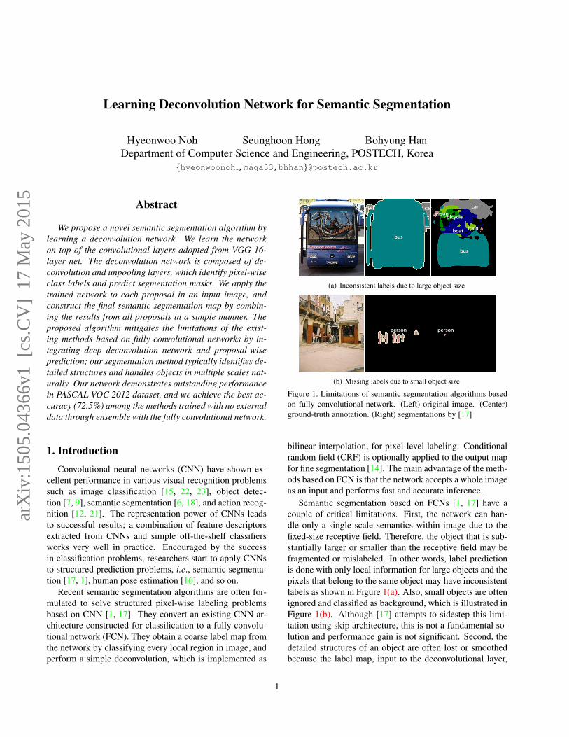
Figure 1. Limitations of semantic segmentation algorithms basedon fully convolutional network. (Left) original image. (Center)ground-truth annotation. (Right) segmentations by [17]

bilinear interpolation, for pixel-level labeling. Conditionalrandom field (CRF) is optionally applied to the output mapfor fine segmentation [14]. The main advantage of the meth-ods based on FCN is that the network accepts a whole imageas an input and performs fast and accurate inference.

Semantic segmentation based on FCNs [1, 17] have acouple of critical limitations. First, the network can han-dle only a single scale semantics within image due to thefixed-size receptive field. Therefore, the object that is sub-stantially larger or smaller than the receptive field may befragmented or mislabeled. In other words, label predictionis done with only local information for large objects and thepixels that belong to the same object may have inconsistentlabels as shown in Figure 1(a). Also, small objects are oftenignored and classified as background, which is illustrated inFigure 1(b). Although [17] attempts to sidestep this limi-tation using skip architecture, this is not a fundamental so-lution and performance gain is not significant. Second, thedetailed structures of an object are often lost or smoothedbecause the label map, input to the deconvolutional layer,

1

arX

iv:1

505.

0436

6v1

[cs

.CV

] 1

7 M

ay 2

015

is too coarse and deconvolution procedure is overly sim-ple. Note that, in the original FCN [17], the label map isonly 16 × 16 in size and is deconvolved to generate seg-mentation result in the original input size through bilinearinterpolation. The absence of real deconvolution in [1, 17]makes it difficult to achieve good performance. However,recent methods ameliorate this problem using CRF [14].

To overcome such limitations, we employ a completelydifferent strategy to perform semantic segmentation basedon CNN. Our main contributions are summarized below:

• We learn a multi-layer deconvolution network, whichis composed of deconvolution, unpooling, and rectifiedlinear unit (ReLU) layers. Learning deconvolution net-work for semantic segmentation is meaningful but noone has attempted to do it yet to our knowledge.

• The trained network is applied to individual object pro-posals to obtain instance-wise segmentations, whichare combined for the final semantic segmentation; itis free from scale issues found in FCN-based methodsand identifies finer details of an object.

• We achieve outstanding performance using the decon-volution network trained only on PASCAL VOC 2012dataset, and obtain the best accuracy through the en-semble with [17] by exploiting the heterogeneous andcomplementary characteristics of our algorithm withrespect to FCN-based methods.

We believe that all of these three contributions help achievethe state-of-the-art performance in PASCAL VOC 2012benchmark.

The rest of this paper is organized as follows. We firstreview related work in Section 2 and describe the architec-ture of our network in Section 3. The detailed procedureto learn a supervised deconvolution network is discussedin Section 4. Section 5 presents how to utilize the learneddeconvolution network for semantic segmentation. Experi-mental results are demonstrated in Section 6.

2. Related Work

CNNs are very popular in many visual recognition prob-lems and have also been applied to semantic segmentationactively. We first summarize the existing algorithms basedon supervised learning for semantic segmentation.

There are several semantic segmentation methods basedon classification. Mostajabi et al. [18] and Farabet et al. [6]classify multi-scale superpixels into predefined categoriesand combine the classification results for pixel-wise label-ing. Some algorithms [3, 9, 10] classify region proposalsand refine the labels in the image-level segmentation mapto obtain the final segmentation.

Fully convolutional network (FCN) [17] has driven re-cent breakthrough on deep learning based semantic seg-mentation. In this approach, fully connected layers in thestandard CNNs are interpreted as convolutions with largereceptive fields, and segmentation is achieved using coarseclass score maps obtained by feedforwarding an input im-age. An interesting idea in this work is that a simple inter-polation filter is employed for deconvolution and only theCNN part of the network is fine-tuned to learn deconvolu-tion indirectly. Surprisingly, the output network illustratesimpressive performance on the PASCAL VOC benchmark.Chen et al. [1] obtain denser score maps within the FCNframework to predict pixel-wise labels and refine the labelmap using the fully connected CRF [14].

In addition to the methods based on supervised learning,several semantic segmentation techniques in weakly super-vised settings have been proposed. When only boundingbox annotations are given for input images, [2, 19] refinethe annotations through iterative procedures and obtain ac-curate segmentation outputs. On the other hand, [20] per-forms semantic segmentation based only on image-level an-notations in a multiple instance learning framework.

Semantic segmentation involves deconvolution concep-tually, but learning deconvolution network is not very com-mon. Deconvolution network is introduced in [25] to re-construct input images. As the reconstruction of an inputimage is non-trivial due to max pooling layers, it proposesthe unpooling operation by storing the pooled location. Us-ing the deconvoluton network, the input image can be re-constructed from its feature representation. This approachis also employed to visualize activated features in a trainedCNN [24] and update network architecture for performanceenhancement. This visualization is useful for understandingthe behavior of a trained CNN model.

3. System Architecture

This section discusses the architecture of our deconvolu-tion network, and describes the overall semantic segmenta-tion algorithm.

3.1. Architecture

Figure 2 illustrates the detailed configuration of the en-tire deep network. Our trained network is composed of twoparts—convolution and deconvolution networks. The con-volution network corresponds to feature extractor that trans-forms the input image to multidimensional feature represen-tation, whereas the deconvolution network is a shape gen-erator that produces object segmentation from the featureextracted from the convolution network. The final output ofthe network is a probability map in the same size to inputimage, indicating probability of each pixel that belongs toone of the predefined classes.

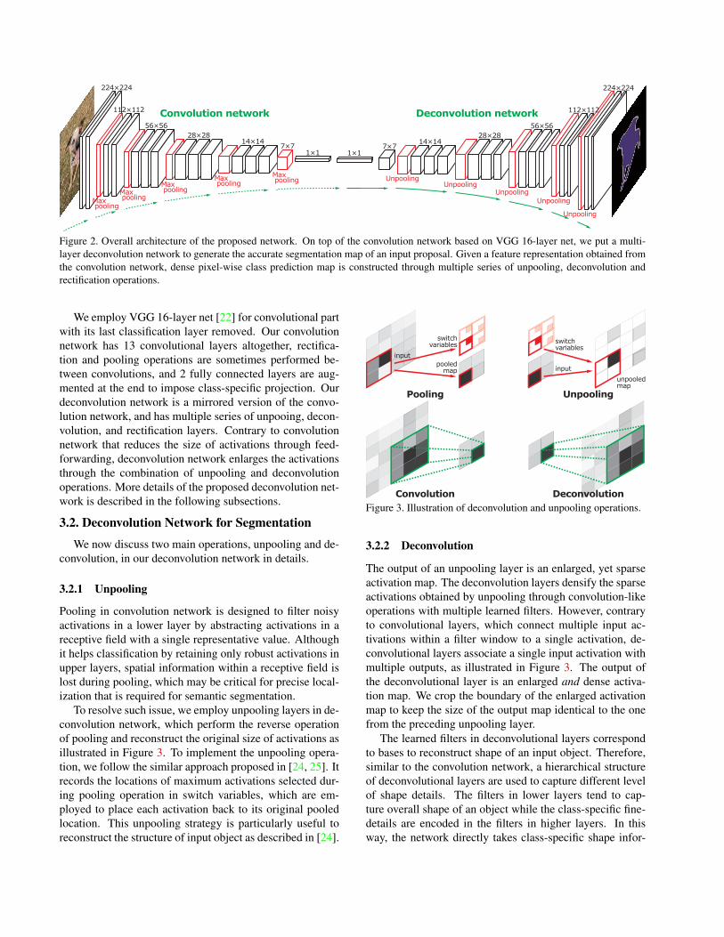
Figure 2. Overall architecture of the proposed network. On top of the convolution network based on VGG 16-layer net, we put a multi-layer deconvolution network to generate the accurate segmentation map of an input proposal. Given a feature representation obtained fromthe convolution network, dense pixel-wise class prediction map is constructed through multiple series of unpooling, deconvolution andrectification operations.

We employ VGG 16-layer net [22] for convolutional partwith its last classification layer removed. Our convolutionnetwork has 13 convolutional layers altogether, rectifica-tion and pooling operations are sometimes performed be-tween convolutions, and 2 fully connected layers are aug-mented at the end to impose class-specific projection. Ourdeconvolution network is a mirrored version of the convo-lution network, and has multiple series of unpooing, decon-volution, and rectification layers. Contrary to convolutionnetwork that reduces the size of activations through feed-forwarding, deconvolution network enlarges the activationsthrough the combination of unpooling and deconvolutionoperations. More details of the proposed deconvolution net-work is described in the following subsections.

3.2. Deconvolution Network for Segmentation

We now discuss two main operations, unpooling and de-convolution, in our deconvolution network in details.

3.2.1 Unpooling

Pooling in convolution network is designed to filter noisyactivations in a lower layer by abstracting activations in areceptive field with a single representative value. Althoughit helps classification by retaining only robust activations inupper layers, spatial information within a receptive field islost during pooling, which may be critical for precise local-ization that is required for semantic segmentation.

To resolve such issue, we employ unpooling layers in de-convolution network, which perform the reverse operationof pooling and reconstruct the original size of activations asillustrated in Figure 3. To implement the unpooling opera-tion, we follow the similar approach proposed in [24, 25]. Itrecords the locations of maximum activations selected dur-ing pooling operation in switch variables, which are em-ployed to place each activation back to its original pooledlocation. This unpooling strategy is particularly useful toreconstruct the structure of input object as described in [24].

Figure 3. Illustration of deconvolution and unpooling operations.

3.2.2 Deconvolution

The output of an unpooling layer is an enlarged, yet sparseactivation map. The deconvolution layers densify the sparseactivations obtained by unpooling through convolution-likeoperations with multiple learned filters. However, contraryto convolutional layers, which connect multiple input ac-tivations within a filter window to a single activation, de-convolutional layers associate a single input activation withmultiple outputs, as illustrated in Figure 3. The output ofthe deconvolutional layer is an enlarged and dense activa-tion map. We crop the boundary of the enlarged activationmap to keep the size of the output map identical to the onefrom the preceding unpooling layer.

The learned filters in deconvolutional layers correspondto bases to reconstruct shape of an input object. Therefore,similar to the convolution network, a hierarchical structureof deconvolutional layers are used to capture different levelof shape details. The filters in lower layers tend to cap-ture overall shape of an object while the class-specific fine-details are encoded in the filters in higher layers. In thisway, the network directly takes class-specific shape infor-

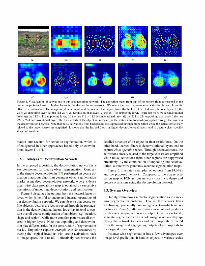
(a) (b) (c) (d) (e)

(f) (g) (h) (i) (j)

Figure 4. Visualization of activations in our deconvolution network. The activation maps from top left to bottom right correspond to theoutput maps from lower to higher layers in the deconvolution network. We select the most representative activation in each layer foreffective visualization. The image in (a) is an input, and the rest are the outputs from (b) the last 14 × 14 deconvolutional layer, (c) the28× 28 unpooling layer, (d) the last 28× 28 deconvolutional layer, (e) the 56× 56 unpooling layer, (f) the last 56× 56 deconvolutionallayer, (g) the 112 × 112 unpooling layer, (h) the last 112 × 112 deconvolutional layer, (i) the 224 × 224 unpooling layer and (j) the last224× 224 deconvolutional layer. The finer details of the object are revealed, as the features are forward-propagated through the layers inthe deconvolution network. Note that noisy activations from background are suppressed through propagation while the activations closelyrelated to the target classes are amplified. It shows that the learned filters in higher deconvolutional layers tend to capture class-specificshape information.

mation into account for semantic segmentation, which isoften ignored in other approaches based only on convolu-tional layers [1, 17].

3.2.3 Analysis of Deconvolution Network

In the proposed algorithm, the deconvolution network is akey component for precise object segmentation. Contraryto the simple deconvolution in [17] performed on coarse ac-tivation maps, our algorithm generates object segmentationmasks using deep deconvolution network, where a densepixel-wise class probability map is obtained by successiveoperations of unpooling, deconvolution, and rectification.

Figure 4 visualizes the outputs from the network layer bylayer, which is helpful to understand internal operations ofour deconvolution network. We can observe that coarse-to-fine object structures are reconstructed through the propaga-tion in the deconvolutional layers; lower layers tend to cap-ture overall coarse configuration of an object (e.g. location,shape and region), while more complex patterns are discov-ered in higher layers. Note that unpooling and deconvolu-tion play different roles for the construction of segmentationmasks. Unpooling captures example-specific structures bytracing the original locations with strong activations backto image space. As a result, it effectively reconstructs the

detailed structure of an object in finer resolutions. On theother hand, learned filters in deconvolutional layers tend tocapture class-specific shapes. Through deconvolutions, theactivations closely related to the target classes are amplifiedwhile noisy activations from other regions are suppressedeffectively. By the combination of unpooling and deconvo-lution, our network generates accurate segmentation maps.

Figure 5 illustrates examples of outputs from FCN-8sand the proposed network. Compared to the coarse acti-vation map of FCN-8s, our network constructs dense andprecise activations using the deconvolution network.

3.3. System Overview

Our algorithm poses semantic segmentation as instance-wise segmentation problem. That is, the network takesa sub-image potentially containing objects—which we re-fer to as instance(s) afterwards—as an input and producespixel-wise class prediction as an output. Given our network,semantic segmentation on a whole image is obtained by ap-plying the network to each candidate proposals extractedfrom the image and aggregating outputs of all proposals tothe original image space.

Instance-wise segmentation has a few advantages overimage-level prediction. It handles objects in various scales

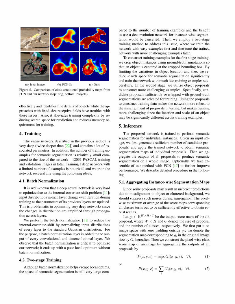
(a) Input image (b) FCN-8s (c) Ours

Figure 5. Comparison of class conditional probability maps fromFCN and our network (top: dog, bottom: bicycle).

effectively and identifies fine details of objects while the ap-proaches with fixed-size receptive fields have troubles withthese issues. Also, it alleviates training complexity by re-ducing search space for prediction and reduces memory re-quirement for training.

4. TrainingThe entire network described in the previous section is

very deep (twice deeper than [22]) and contains a lot of as-sociated parameters. In addition, the number of training ex-amples for semantic segmentation is relatively small com-pared to the size of the network—12031 PASCAL trainingand validation images in total. Training a deep network witha limited number of examples is not trivial and we train thenetwork successfully using the following ideas.

4.1. Batch Normalization

It is well-known that a deep neural network is very hardto optimize due to the internal-covariate-shift problem [11];input distributions in each layer change over iteration duringtraining as the parameters of its previous layers are updated.This is problematic in optimizing very deep networks sincethe changes in distribution are amplified through propaga-tion across layers.

We perform the batch normalization [11] to reduce theinternal-covariate-shift by normalizing input distributionsof every layer to the standard Gaussian distribution. Forthe purpose, a batch normalization layer is added to the out-put of every convolutional and deconvolutional layer. Weobserve that the batch normalization is critical to optimizeour network; it ends up with a poor local optimum withoutbatch normalization.

4.2. Two-stage Training

Although batch normalization helps escape local optima,the space of semantic segmentation is still very large com-

pared to the number of training examples and the benefitto use a deconvolution network for instance-wise segmen-tation would be cancelled. Then, we employ a two-stagetraining method to address this issue, where we train thenetwork with easy examples first and fine-tune the trainednetwork with more challenging examples later.

To construct training examples for the first stage training,we crop object instances using ground-truth annotations sothat an object is centered at the cropped bounding box. Bylimiting the variations in object location and size, we re-duce search space for semantic segmentation significantlyand train the network with much less training examples suc-cessfully. In the second stage, we utilize object proposalsto construct more challenging examples. Specifically, can-didate proposals sufficiently overlapped with ground-truthsegmentations are selected for training. Using the proposalsto construct training data makes the network more robust tothe misalignment of proposals in testing, but makes trainingmore challenging since the location and scale of an objectmay be significantly different across training examples.

5. InferenceThe proposed network is trained to perform semantic

segmentation for individual instances. Given an input im-age, we first generate a sufficient number of candidate pro-posals, and apply the trained network to obtain semanticsegmentation maps of individual proposals. Then we ag-gregate the outputs of all proposals to produce semanticsegmentation on a whole image. Optionally, we take en-semble of our method with FCN [17] to further improveperformance. We describe detailed procedure in the follow-ing.

5.1. Aggregating Instance-wise Segmentation Maps

Since some proposals may result in incorrect predictionsdue to misalignment to object or cluttered background, weshould suppress such noises during aggregation. The pixel-wise maximum or average of the score maps correspondingall classes turns out to be sufficiently effective to obtain ro-bust results.

Let gi ∈ RW×H×C be the output score maps of the ithproposal, where W ×H and C denote the size of proposaland the number of classes, respectively. We first put it onimage space with zero padding outside gi; we denote thesegmentation map corresponding to gi in the original imagesize by Gi hereafter. Then we construct the pixel-wise classscore map of an image by aggregating the outputs of allproposals by

P (x, y, c) = maxi

Gi(x, y, c), ∀i, (1)

orP (x, y, c) =

∑i

Gi(x, y, c), ∀i. (2)

Class conditional probability maps in the original imagespace are obtained by applying softmax function to the ag-gregated maps obtained by Eq. (1) or (2). Finally, we applythe fully-connected CRF [14] to the output maps for the fi-nal pixel-wise labeling, where unary potential are obtainedfrom the pixel-wise class conditional probability maps.

5.2. Ensemble with FCN

Our algorithm based on the deconvolution network hascomplementary characteristics to the approaches relying onFCN; our deconvolution network is appropriate to capturethe fine-details of an object, whereas FCN is typically goodat extracting the overall shape of an object. In addition,instance-wise prediction is useful for handling objects withvarious scales, while fully convolutional network with acoarse scale may be advantageous to capture context withinimage. Exploiting these heterogeneous properties may leadto better results, and we take advantage of the benefit ofboth algorithms through ensemble.

We develop a simple method to combine the outputs ofboth algorithms. Given two sets of class conditional prob-ability maps of an input image computed independently bythe proposed method and FCN, we compute the mean ofboth output maps and apply the CRF to obtain the final se-mantic segmentation.

6. Experiments

This section first describes our implementation detailsand experiment setup. Then, we analyze and evaluate theproposed network in various aspects.

6.1. Implementation Details

Network Configuration Table 2 summarizes the detailedconfiguration of the proposed network presented in Fig-ure 2. Our network has symmetrical configuration of convo-lution and deconvolution network centered around the 2ndfully-connected layer (fc7). The input and output layerscorrespond to input image and class conditional probabil-ity maps, respectively. The network contains approximately252M parameters in total.

Dataset We employ PASCAL VOC 2012 segmentationdataset [5] for training and testing the proposed deep net-work. For training, we use augmented segmentation annota-tions from [8], where all training and validation images areused to train our network. The performance of our networkis evaluated on test images. Note that only the images inPASCAL VOC 2012 datasets are used for training in our ex-periment, whereas some state-of-the-art algorithms [2, 19]employ additional data to improve performance.

Training Data Construction We employ a two-stagetraining strategy and use a separate training dataset in eachstage. To construct training examples for the first stage,we draw a tight bounding box corresponding to each anno-tated object in training images, and extend the box 1.2 timeslarger to include local context around the object. Then wecrop the window using the extended bounding box to obtaina training example. The class label for each cropped regionis provided based only on the object located at the centerwhile all other pixels are labeled as background. In the sec-ond stage, each training example is extracted from objectproposal [26], where all relevant class labels are used forannotation. We employ the same post-processing as the oneused in the first stage to include context. For both datasets,we maintain the balance for the number of examples acrossclasses by adding redundant examples for the classes withlimited number of examples. To augment training data, wetransform an input example to a 250 × 250 image and ran-domly crop the image to 224×224 with optional horizontalflipping in a similar way to [22]. The number of training ex-amples is 0.2M and 2.7M in the first and the second stage,respectively, which is sufficiently large to train the decon-volution network from scratch.

Optmization We implement the proposed network basedon Caffe [13] framework. The standard stochastic gradi-ent descent with momentum is employed for optimization,where initial learning rate, momentum and weight decay areset to 0.01, 0.9 and 0,0005, respectively. We initialize theweights in the convolution network using VGG 16-layer netpre-trained on ILSVRC [4] dataset, while the weights in thedeconvolution network are initialized with zero-mean Gaus-sians. We remove the drop-out layers due to batch normal-ization, and reduce learning rate in an order of magnitudewhenever validation accuracy does not improve. Althoughour final network is learned with both train and validationdatasets, learning rate adjustment based on validation ac-curacy still works well according to our experience. Thenetwork converges after approximately 20K and 40K SGDiterations with mini-batch of 64 samples in the first and sec-ond stage training, respectively. Training takes 6 days (2days for the first stage and 4 days for the second stage) in asingle Nvidia GTX Titan X GPU with 12G memory.

Inference We employ edge-box [26] to generate objectproposals. For each testing image, we generate approxi-mately 2000 object proposals, and select top 50 proposalsbased on their objectness scores. We observe that this num-ber is sufficient to obtain accurate segmentation in practice.To obtain pixel-wise class conditional probability maps fora whole image, we compute pixel-wise maximum to aggre-gate proposal-wise predictions as in Eq. (1).

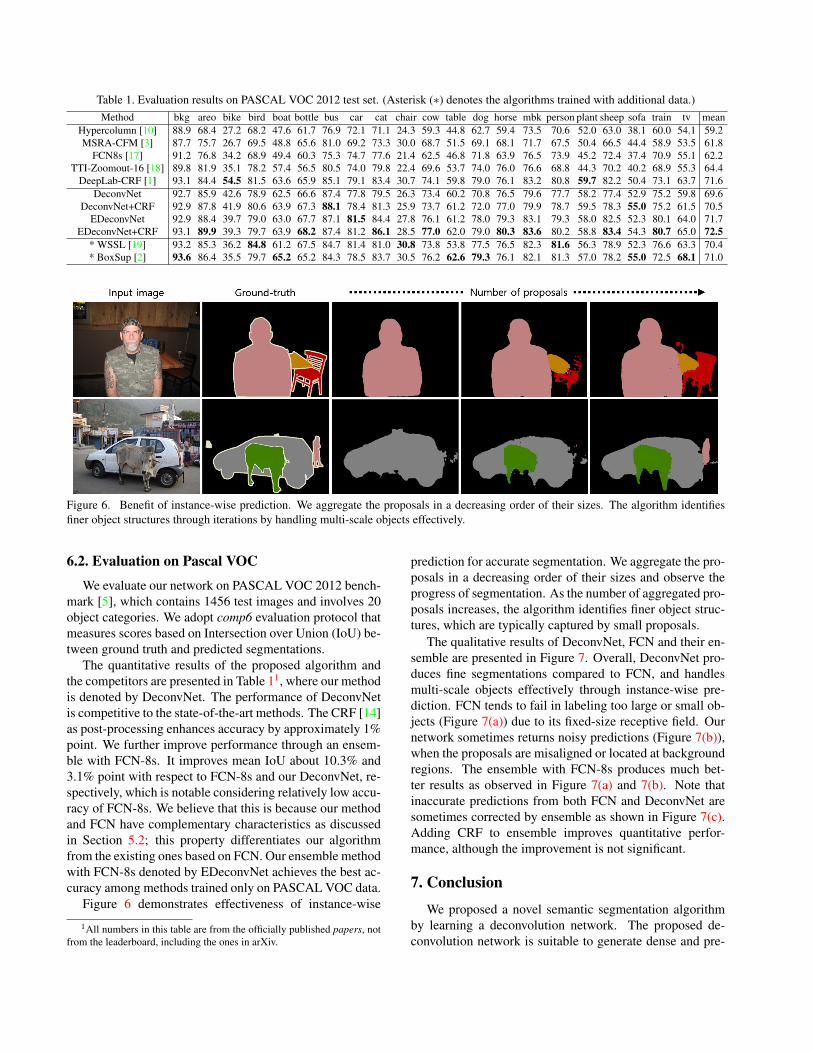
Table 1. Evaluation results on PASCAL VOC 2012 test set. (Asterisk (∗) denotes the algorithms trained with additional data.)Method bkg areo bike bird boat bottle bus car cat chair cow table dog horse mbk person plant sheep sofa train tv mean

Hypercolumn [10] 88.9 68.4 27.2 68.2 47.6 61.7 76.9 72.1 71.1 24.3 59.3 44.8 62.7 59.4 73.5 70.6 52.0 63.0 38.1 60.0 54.1 59.2MSRA-CFM [3] 87.7 75.7 26.7 69.5 48.8 65.6 81.0 69.2 73.3 30.0 68.7 51.5 69.1 68.1 71.7 67.5 50.4 66.5 44.4 58.9 53.5 61.8

FCN8s [17] 91.2 76.8 34.2 68.9 49.4 60.3 75.3 74.7 77.6 21.4 62.5 46.8 71.8 63.9 76.5 73.9 45.2 72.4 37.4 70.9 55.1 62.2TTI-Zoomout-16 [18] 89.8 81.9 35.1 78.2 57.4 56.5 80.5 74.0 79.8 22.4 69.6 53.7 74.0 76.0 76.6 68.8 44.3 70.2 40.2 68.9 55.3 64.4

DeepLab-CRF [1] 93.1 84.4 54.5 81.5 63.6 65.9 85.1 79.1 83.4 30.7 74.1 59.8 79.0 76.1 83.2 80.8 59.7 82.2 50.4 73.1 63.7 71.6DeconvNet 92.7 85.9 42.6 78.9 62.5 66.6 87.4 77.8 79.5 26.3 73.4 60.2 70.8 76.5 79.6 77.7 58.2 77.4 52.9 75.2 59.8 69.6

DeconvNet+CRF 92.9 87.8 41.9 80.6 63.9 67.3 88.1 78.4 81.3 25.9 73.7 61.2 72.0 77.0 79.9 78.7 59.5 78.3 55.0 75.2 61.5 70.5EDeconvNet 92.9 88.4 39.7 79.0 63.0 67.7 87.1 81.5 84.4 27.8 76.1 61.2 78.0 79.3 83.1 79.3 58.0 82.5 52.3 80.1 64.0 71.7

EDeconvNet+CRF 93.1 89.9 39.3 79.7 63.9 68.2 87.4 81.2 86.1 28.5 77.0 62.0 79.0 80.3 83.6 80.2 58.8 83.4 54.3 80.7 65.0 72.5* WSSL [19] 93.2 85.3 36.2 84.8 61.2 67.5 84.7 81.4 81.0 30.8 73.8 53.8 77.5 76.5 82.3 81.6 56.3 78.9 52.3 76.6 63.3 70.4* BoxSup [2] 93.6 86.4 35.5 79.7 65.2 65.2 84.3 78.5 83.7 30.5 76.2 62.6 79.3 76.1 82.1 81.3 57.0 78.2 55.0 72.5 68.1 71.0

Figure 6. Benefit of instance-wise prediction. We aggregate the proposals in a decreasing order of their sizes. The algorithm identifiesfiner object structures through iterations by handling multi-scale objects effectively.

6.2. Evaluation on Pascal VOC

We evaluate our network on PASCAL VOC 2012 bench-mark [5], which contains 1456 test images and involves 20object categories. We adopt comp6 evaluation protocol thatmeasures scores based on Intersection over Union (IoU) be-tween ground truth and predicted segmentations.

The quantitative results of the proposed algorithm andthe competitors are presented in Table 11, where our methodis denoted by DeconvNet. The performance of DeconvNetis competitive to the state-of-the-art methods. The CRF [14]as post-processing enhances accuracy by approximately 1%point. We further improve performance through an ensem-ble with FCN-8s. It improves mean IoU about 10.3% and3.1% point with respect to FCN-8s and our DeconvNet, re-spectively, which is notable considering relatively low accu-racy of FCN-8s. We believe that this is because our methodand FCN have complementary characteristics as discussedin Section 5.2; this property differentiates our algorithmfrom the existing ones based on FCN. Our ensemble methodwith FCN-8s denoted by EDeconvNet achieves the best ac-curacy among methods trained only on PASCAL VOC data.

Figure 6 demonstrates effectiveness of instance-wise

1All numbers in this table are from the officially published papers, notfrom the leaderboard, including the ones in arXiv.

prediction for accurate segmentation. We aggregate the pro-posals in a decreasing order of their sizes and observe theprogress of segmentation. As the number of aggregated pro-posals increases, the algorithm identifies finer object struc-tures, which are typically captured by small proposals.

The qualitative results of DeconvNet, FCN and their en-semble are presented in Figure 7. Overall, DeconvNet pro-duces fine segmentations compared to FCN, and handlesmulti-scale objects effectively through instance-wise pre-diction. FCN tends to fail in labeling too large or small ob-jects (Figure 7(a)) due to its fixed-size receptive field. Ournetwork sometimes returns noisy predictions (Figure 7(b)),when the proposals are misaligned or located at backgroundregions. The ensemble with FCN-8s produces much bet-ter results as observed in Figure 7(a) and 7(b). Note thatinaccurate predictions from both FCN and DeconvNet aresometimes corrected by ensemble as shown in Figure 7(c).Adding CRF to ensemble improves quantitative perfor-mance, although the improvement is not significant.

7. Conclusion

We proposed a novel semantic segmentation algorithmby learning a deconvolution network. The proposed de-convolution network is suitable to generate dense and pre-

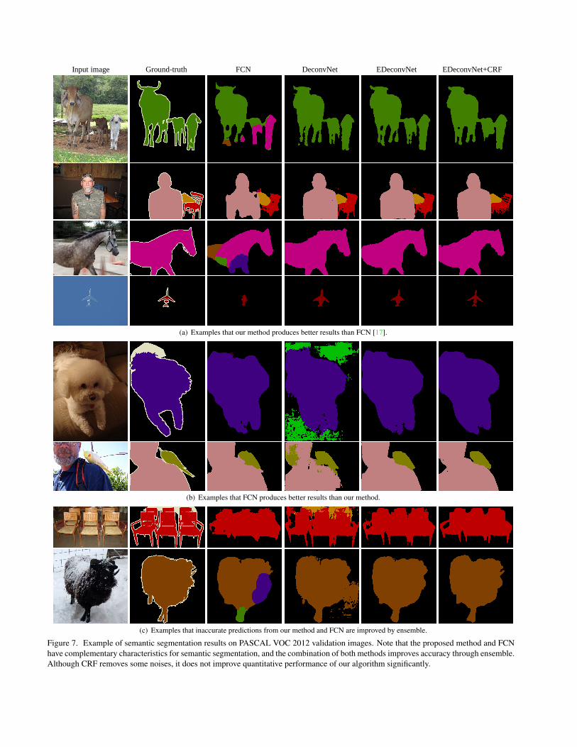
Input image Ground-truth FCN DeconvNet EDeconvNet EDeconvNet+CRF

(a) Examples that our method produces better results than FCN [17].

(b) Examples that FCN produces better results than our method.

(c) Examples that inaccurate predictions from our method and FCN are improved by ensemble.

Figure 7. Example of semantic segmentation results on PASCAL VOC 2012 validation images. Note that the proposed method and FCNhave complementary characteristics for semantic segmentation, and the combination of both methods improves accuracy through ensemble.Although CRF removes some noises, it does not improve quantitative performance of our algorithm significantly.

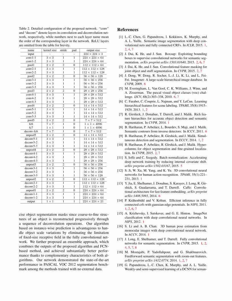
Table 2. Detailed configuration of the proposed network. “conv”and “deconv” denote layers in convolution and deconvolution net-work, respectively, while numbers next to each layer name meanthe order of the corresponding layer in the network. ReLU layersare omitted from the table for brevity.

name kernel size stride pad output sizeinput - - - 224× 224× 3

conv1-1 3× 3 1 1 224× 224× 64conv1-2 3× 3 1 1 224× 224× 64pool1 2× 2 2 0 112× 112× 64

conv2-1 3× 3 1 1 112× 112× 128conv2-2 3× 3 1 1 112× 112× 128pool2 2× 2 2 0 56× 56× 128

conv3-1 3× 3 1 1 56× 56× 256conv3-2 3× 3 1 1 56× 56× 256conv3-3 3× 3 1 1 56× 56× 256pool3 2× 2 2 0 28× 28× 256

conv4-1 3× 3 1 1 28× 28× 512conv4-2 3× 3 1 1 28× 28× 512conv4-3 3× 3 1 1 28× 28× 512pool4 2× 2 2 0 14× 14× 512

conv5-1 3× 3 1 1 14× 14× 512conv5-2 3× 3 1 1 14× 14× 512conv5-3 3× 3 1 1 14× 14× 512pool5 2× 2 2 0 7× 7× 512

fc6 7× 7 1 0 1× 1× 4096fc7 1× 1 1 0 1× 1× 4096

deconv-fc6 7× 7 1 0 7× 7× 512unpool5 2× 2 2 0 14× 14× 512

deconv5-1 3× 3 1 1 14× 14× 512deconv5-2 3× 3 1 1 14× 14× 512deconv5-3 3× 3 1 1 14× 14× 512unpool4 2× 2 2 0 28× 28× 512

deconv4-1 3× 3 1 1 28× 28× 512deconv4-2 3× 3 1 1 28× 28× 512deconv4-3 3× 3 1 1 28× 28× 256unpool3 2× 2 2 0 56× 56× 256

deconv3-1 3× 3 1 1 56× 56× 256deconv3-2 3× 3 1 1 56× 56× 256deconv3-3 3× 3 1 1 56× 56× 128unpool2 2× 2 2 0 112× 112× 128

deconv2-1 3× 3 1 1 112× 112× 128deconv2-2 3× 3 1 1 112× 112× 64unpool1 2× 2 2 0 224× 224× 64

deconv1-1 3× 3 1 1 224× 224× 64deconv1-2 3× 3 1 1 224× 224× 64

output 1× 1 1 1 224× 224× 21

cise object segmentation masks since coarse-to-fine struc-tures of an object is reconstructed progressively througha sequence of deconvolution operations. Our algorithmbased on instance-wise prediction is advantageous to han-dle object scale variations by eliminating the limitationof fixed-size receptive field in the fully convolutional net-work. We further proposed an ensemble approach, whichcombines the outputs of the proposed algorithm and FCN-based method, and achieved substantially better perfor-mance thanks to complementary characteristics of both al-gorithms. Our network demonstrated the state-of-the-artperformance in PASCAL VOC 2012 segmentation bench-mark among the methods trained with no external data.

References[1] L.-C. Chen, G. Papandreou, I. Kokkinos, K. Murphy, and

A. L. Yuille. Semantic image segmentation with deep con-volutional nets and fully connected CRFs. In ICLR, 2015. 1,2, 4, 7

[2] J. Dai, K. He, and J. Sun. Boxsup: Exploiting boundingboxes to supervise convolutional networks for semantic seg-mentation. arXiv preprint arXiv:1503.01640, 2015. 2, 6, 7

[3] J. Dai, K. He, and J. Sun. Convolutional feature masking forjoint object and stuff segmentation. In CVPR, 2015. 2, 7

[4] J. Deng, W. Dong, R. Socher, L.-J. Li, K. Li, and L. Fei-Fei. Imagenet: A large-scale hierarchical image database. InCVPR, 2009. 6

[5] M. Everingham, L. Van Gool, C. K. Williams, J. Winn, andA. Zisserman. The pascal visual object classes (voc) chal-lenge. IJCV, 88(2):303–338, 2010. 6, 7

[6] C. Farabet, C. Couprie, L. Najman, and Y. LeCun. Learninghierarchical features for scene labeling. TPAMI, 35(8):1915–1929, 2013. 1, 2

[7] R. Girshick, J. Donahue, T. Darrell, and J. Malik. Rich fea-ture hierarchies for accurate object detection and semanticsegmentation. In CVPR, 2014. 1

[8] B. Hariharan, P. Arbelaez, L. Bourdev, S. Maji, and J. Malik.Semantic contours from inverse detectors. In ICCV, 2011. 6

[9] B. Hariharan, P. Arbelaez, R. Girshick, and J. Malik. Simul-taneous detection and segmentation. In ECCV, 2014. 1, 2

[10] B. Hariharan, P. Arbelaez, R. Girshick, and J. Malik. Hyper-columns for object segmentation and fine-grained localiza-tion. In CVPR, 2015. 2, 7

[11] S. Ioffe and C. Szegedy. Batch normalization: Acceleratingdeep network training by reducing internal covariate shift.arXiv preprint arXiv:1502.03167, 2015. 5

[12] S. Ji, W. Xu, M. Yang, and K. Yu. 3D convolutional neuralnetworks for human action recognition. TPAMI, 35(1):221–231, 2013. 1

[13] Y. Jia, E. Shelhamer, J. Donahue, S. Karayev, J. Long, R. Gir-shick, S. Guadarrama, and T. Darrell. Caffe: Convolu-tional architecture for fast feature embedding. arXiv preprintarXiv:1408.5093, 2014. 6

[14] P. Krahenbuhl and V. Koltun. Efficient inference in fullyconnected crfs with gaussian edge potentials. In NIPS, 2011.1, 2, 6, 7

[15] A. Krizhevsky, I. Sutskever, and G. E. Hinton. ImageNetclassification with deep convolutional neural networks. InNIPS, 2012. 1

[16] S. Li and A. B. Chan. 3D human pose estimation frommonocular images with deep convolutional neural network.In ACCV, 2014. 1

[17] J. Long, E. Shelhamer, and T. Darrell. Fully convolutionalnetworks for semantic segmentation. In CVPR, 2015. 1, 2,4, 5, 7, 8

[18] M. Mostajabi, P. Yadollahpour, and G. Shakhnarovich.Feedforward semantic segmentation with zoom-out features.arXiv preprint arXiv:1412.0774, 2014. 1, 2, 7

[19] G. Papandreou, L.-C. Chen, K. Murphy, and A. L. Yuille.Weakly-and semi-supervised learning of a DCNN for seman-

tic image segmentation. arXiv preprint arXiv:1502.02734,2015. 2, 6, 7

[20] P. O. Pinheiro and R. Collobert. Weakly supervised semanticsegmentation with convolutional networks. In CVPR, 2015.2

[21] K. Simonyan and A. Zisserman. Two-stream convolutionalnetworks for action recognition in videos. In NIPS, 2014. 1

[22] K. Simonyan and A. Zisserman. Very deep convolutionalnetworks for large-scale image recognition. In ICLR, 2015.1, 3, 5, 6

[23] C. Szegedy, W. Liu, Y. Jia, P. Sermanet, S. Reed,D. Anguelov, D. Erhan, V. Vanhoucke, and A. Rabi-novich. Going deeper with convolutions. arXiv preprintarXiv:1409.4842, 2014. 1

[24] M. D. Zeiler and R. Fergus. Visualizing and understandingconvolutional networks. In ECCV, 2014. 2, 3

[25] M. D. Zeiler, G. W. Taylor, and R. Fergus. Adaptive decon-volutional networks for mid and high level feature learning.In ICCV, 2011. 2, 3

[26] C. L. Zitnick and P. Dollar. Edge boxes: Locating objectproposals from edges. In ECCV, 2014. 6