The coalescent Understanding genetic variation

Philip Awadalla University of Montreal

Making sense of genetic variation

•  Is there an association between DNA sequence variation and the disease phenotype?

•  What do the sequences tell us about human history?

•  How has natural selection shaped diversity in the gene?

DNA sequence diversity in a 9.7-kb region of the human lipoprotein lipase gene Nickerson, et al. 1998 Nature Genetics 19, 233 - 240

Afr

ican

A

mer

ican

s Fi

nns

Nat

ive

A

mer

ican

s

The aims of population genetics

•  To understand the link between genetic variation and phenotypic variation –  Is variation at this gene associated with disease susceptibility? –  Which loci contribute the variation in hair colour?

•  To investigate the evolutionary history of a species –  How long have these populations been separate? –  Which genes have experienced recent adaptive evolution?

•  To learn about fundamental biological processes –  How does the recombination rate vary along the genome? –  What determines the mutation rate?

The raw material of population genetics

•  Population genetics is the study of naturally occuring genetic variation

•  Genetic variation comes in all shapes and sizes –  Re-sequencing v. SNPs v. microsatellites –  Recombining v. partially linked v. unlinked markers –  Single gene v. multiple loci v. whole genome –  Single population v. multiple population v. multiple species

•  Which data type you collect (and analyse) depends on the questions you want to ask

An example: structuring of human populations

•  Questions –  Is there significant natural structuring to genetic variation in humans? –  Does this structuring coincide with geographical boundaries?

•  Data –  377 autosomal microsatellite loci in 1056 individuals from 52 populations.

Rosenberg et al (2002)

•  Model –  K ‘Hidden’ populations in linkage and Hardy-Weinberg equilibrium

•  Estimation –  Estimate population allele frequencies –  Most likely value of K –  Posterior probability for each individual

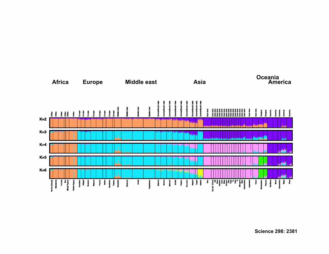
America Oceania

Asia Middle east Europe Africa

Science 298: 2381

Human Population Structure Globally

Population structure at antigens vs. genome-wide

Genome-wide SNPs

Erythocyte Binding Antigens

An example: recombination rates in humans

•  Questions –  How does the recombination rate vary over kilobase scales in humans? –  What is the frequency of recombination hotspots?

•  Data –  Several thousand SNPs typed across a 10Mb region of chromosome 20

(McVean et al 2004) in two populations

•  Model –  Coalescent model of recombination in a single population

•  Estimation –  MCMC scheme for estimating and representing uncertainty

0.001

0.01

0.1

1

10

100

39000 41000 43000 45000 47000 49000

A

Sex-

aver

aged

reco

mbi

natio

n

rate

(cM

/Mb)

NCOA3

Position

Science 304: 581

How do we make sense of data?

•  There are two basic ways of looking at data

•  Nonparametric methods try to say things without relying on models

•  Parametric methods make explicit models for the data

•  For example, in phylogenetics, some people use parsimony (a nonparametric approach) and others use likelihood (a parametric approach) to estimating trees

•  In population genetics, we will come across nonparametric methods (for example in looking at recombination), but most methods are model-based

Parametric

•  Explicit form of underlying distribution is assumed

•  Model characterised by parameters

•  Use of model allows precise statements to be made

•  Inferences and predictions are wrong if model is wrong!

•  Explicit form of underlying distribution is NOT assumed (though certain features may be – e.g. symmetry)

•  Distribution characterised by moments and empirical CDF

•  Greater robustness at expense of power

•  Inferences and predictions independent of exact underlying process

Non-parametric

Population genetic inference

Selection

Mutation

Genetic drift

Recombination

Migration

Evolutionary parameters Population Sample

Stochastic Evolutionary

process

ATGCATGGGCTATTGGACCT

ATGGATGGGCTATTGCACCT

ATGCATGGGCAATTGCACCT

ATGCATGGGCAATTGGACCT

ATGGATGGGCTATTGCACCT

Stochastic Sampling

process

Inference

The basic model of population genetics

Nothing interesting ever happens in biology

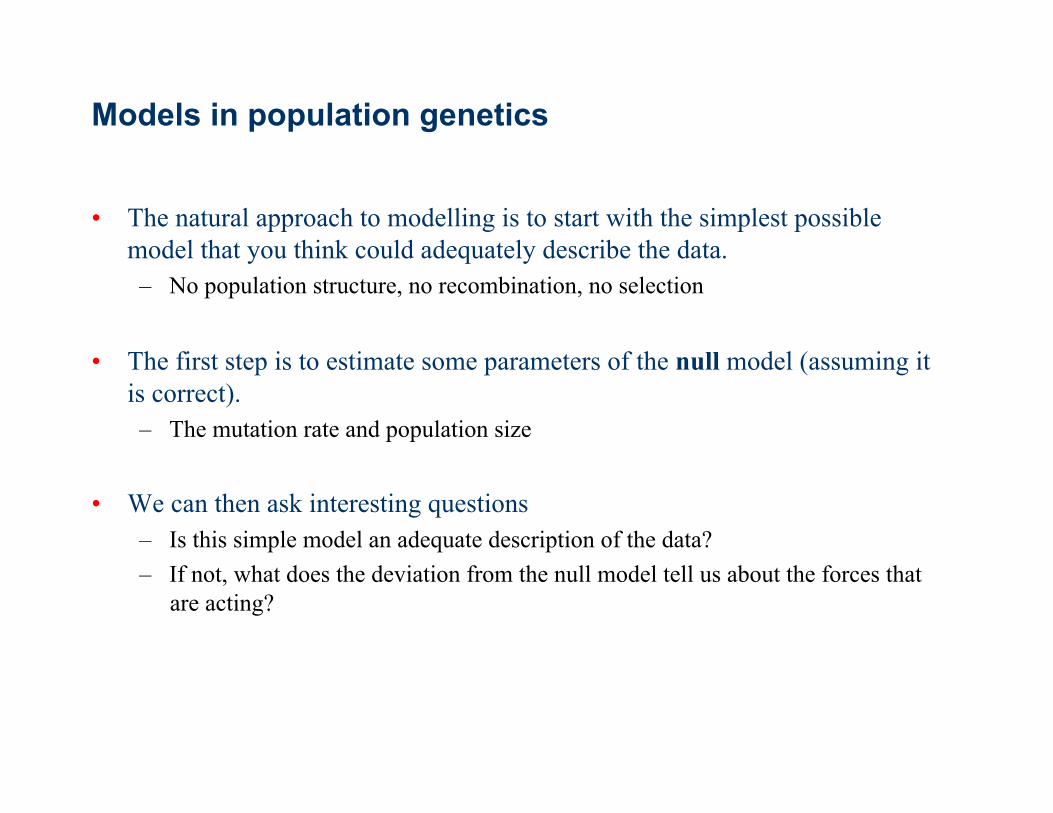
Models in population genetics

•  The natural approach to modelling is to start with the simplest possible model that you think could adequately describe the data. –  No population structure, no recombination, no selection

•  The first step is to estimate some parameters of the null model (assuming it is correct). –  The mutation rate and population size

•  We can then ask interesting questions –  Is this simple model an adequate description of the data? –  If not, what does the deviation from the null model tell us about the forces that

are acting?

Statistical inference

Define model

Explore properties

Estimate parameters from data

Test goodness-of-fit

Refine model

rules parameters simulation

summary statistics graphical representation

moment methods likelihood

outliers heterogeneity

comparison of estimators

Issues

add parameters

The unusual nature of population genetic data

•  Conventional statistical inference –  Many independent data points –  Sample space of low dimensions –  Analytical formulations for inference using all possible information often

possible

•  Population genetic data –  Typically a single draw from the evolutionary process –  Sample space of many dimensions –  Analytical formulations for inference using ALL possible information usually

impossible to derive

The Wright-Fisher population model

N0 Nt N1 N2 N3

•  Diploid Individuals reproduce by sexual reproduction with possibility of selfing

•  Mating is random with respect to location and genotype

•  Generations are non-overlapping (everyone reproduces simultaneously)

•  The population size is constant of size N (2N alleles)

•  There is no migration or selection

Genes in populations

Present day

Ancestry of current population

Present day

Ancestry of sample

Present day

The coalescent: samples in populations

time

coalescence Most recent common ancestor (MRCA)

Ancestral lineages

Present day

Characteristics of the coalescent

•  The coalescent is a mathematical description of the genealogical process arising in idealised populations

•  It focuses on the genealogy (or tree) underlying the history of a sample of chromosomes

•  It is a probabilistic model, which implies that it describes the distribution of genealogies

•  The principle idea is that the genealogy holds all the information we could ever know about our population and its biology –  We don’t know the genealogy, but if we did, inference would be simple

The coalescent for two sequences

•  Consider the coalescent process for two sequences

•  In one generation, these two sequences either came from the same parent chromosome, i.e. coalesced, (with probability 1/2N) or didn’t (with probability 1-1/2N)

•  The probability of coalescence t generations ago is just

NN

t

21

211

1−

⎟⎠⎞⎜

⎝⎛ −=

Not coalesced for first t-1 generations Coalesce in next

generation

The distribution of coalescence times

•  In the case of discrete generations, the coalescence times takes a geometric distribution

•  In the continuous time limit, which is really what coalescence theory deals with, the distribution of coalescence times takes an exponential distribution (time is scaled in units of 2N generations)

1

1][ =MRCATE

1 2 3

Time of coalescence

pdf

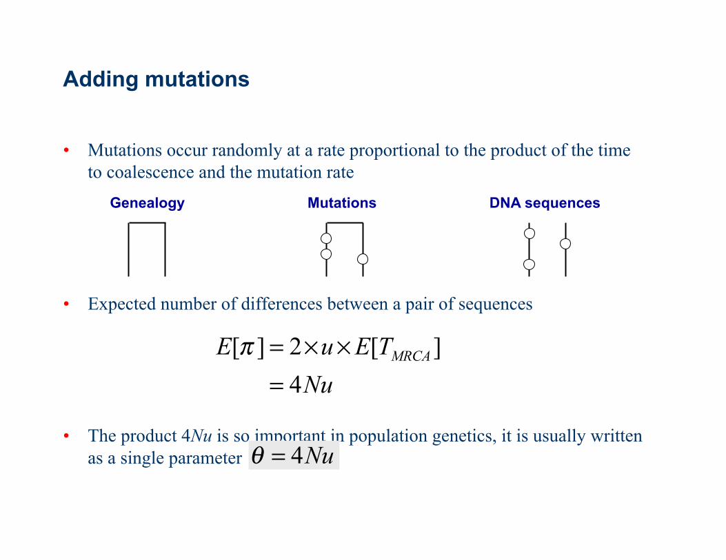
Adding mutations

•  Mutations occur randomly at a rate proportional to the product of the time to coalescence and the mutation rate

•  Expected number of differences between a pair of sequences

•  The product 4Nu is so important in population genetics, it is usually written as a single parameter

Genealogy DNA sequences Mutations

NuTEuE MRCA

4][2][

=××=π

Nu4=θ

The n-coalescent

•  Assume –  Lineages coalesce independently –  No more than one coalescent event can occur in a single generation: in

effect

Genealogy

Sample

∞→eN

time

Coalescence times with n sequences

eNnnn

21

2)1(lineages} given ecoalescencPr{ −=

Number of pairs of lineages Probability of a given pair coalescing

•  When there are n sequences (as opposed to two) it is assumed that each of the n(n-1)/2 pairs coalesce independently

•  This means that the time until the first coalescence is exponentially distributed with rate n(n-1)/2

•  The process is Markov, which means that after the first coalescence, it is like starting again for n-1 sequences

Simulating coalescent histories

•  Stochastic (or Monte Carlo) simulation can be used to learn about the distribution of coalescent histories –  www.coalescent.dk

•  We learn that coalescent genealogies are very variable!

•  Much of the variation in the depth of the tree is due to variation in the time for the last coalescent event to occur

Expected times and mutations

)1(4][−

=nnNTE e

co

unTEE co ××= ][mutations] no.[

Number lineages Total mutation rate

1−=nθ

•  The expected time until the next coalescence is

•  So, the expected number of mutations that occur in the genealogy during this time is

•  Because it is a Markov process, we can just add up the expected number of mutations contributed by each step in the coalescent tree

Properties of the n-coalescent

•  The expected total number of segregating sites is the sum over each coalescent interval

•  The expected time until the MRCA for n sequences is

∑−

=

=1

1

1][n

i iSE θ Watterson (1975)

⎟⎠⎞⎜

⎝⎛ −=

nNTE eMRCA

114][

0 20 40 60 80 100Sample size

1 ][ MRCATE

][SERelative value

Mutations, alleles and haplotypes

•  Infinite-allele model –  Each mutation creates a new allele –  Equivalent to a new haplotype if NO recombination

•  Microsatellites –  Step-wise mutation model

+1

+1

-1

+1 -1 µeNLVarE =)]([

Moran (1975) Slatkin (1995)

ènè......

èè

èèKE

+−++

++

++=

1211][

Ewens (1972)

Summary

•  Population genetics is the study of naturally occurring genetic variation

•  Model-based estimation can be a powerful tool in learning about the forces important in shaping diversity

•  The coalescent is a null model for describing the distribution of genetic variation in samples from unrelated individuals in idealised populations

•  The key idea is that the underlying genealogy relating sequences in a sample is the fundamental quantity of interest

•  The model captures the variability in gene genealogies and, by mapping neutral mutation process on top of the genealogy, patterns of variation

Statistical inference

Define model

Explore properties

Estimate parameters from data

Test goodness-of-fit

Refine model

rules parameters simulation

summary statistics graphical representation

moment methods likelihood

outliers heterogeneity

comparison of estimators

Issues

add parameters

What next?

•  We have a model for genetic variation, now we want to use it to learn things about real data

•  We need to ask two central questions –  Suppose the model is correct, what does the data tell us about the parameters of

the model? –  Does the model provide an accurate description of the data?

•  How do we ask them? –  We need to summarise the data in a way that is informative about the

parameters of the model and model adequacy –  We need to learn about the distribution of those summaries under the model (so

that we can ask if our observations are unusual)

Summarising data

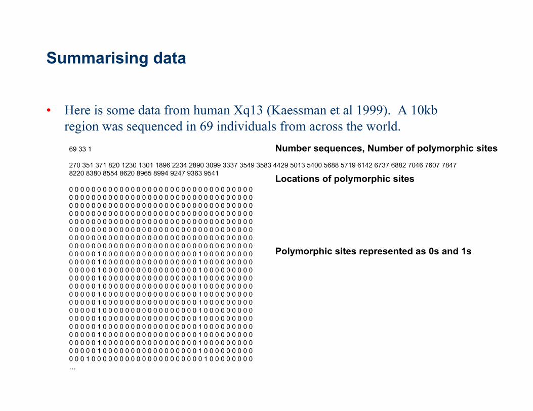
•  Here is some data from human Xq13 (Kaessman et al 1999). A 10kb region was sequenced in 69 individuals from across the world.

69 33 1

270 351 371 820 1230 1301 1896 2234 2890 3099 3337 3549 3583 4429 5013 5400 5688 5719 6142 6737 6882 7046 7607 7847 8220 8380 8554 8620 8965 8994 9247 9363 9541

0 0 0 0 0 0 0 0 0 0 0 0 0 0 0 0 0 0 0 0 0 0 0 0 0 0 0 0 0 0 0 0 0 0 0 0 0 0 0 0 0 0 0 0 0 0 0 0 0 0 0 0 0 0 0 0 0 0 0 0 0 0 0 0 0 0 0 0 0 0 0 0 0 0 0 0 0 0 0 0 0 0 0 0 0 0 0 0 0 0 0 0 0 0 0 0 0 0 0 0 0 0 0 0 0 0 0 0 0 0 0 0 0 0 0 0 0 0 0 0 0 0 0 0 0 0 0 0 0 0 0 0 0 0 0 0 0 0 0 0 0 0 0 0 0 0 0 0 0 0 0 0 0 0 0 0 0 0 0 0 0 0 0 0 0 0 0 0 0 0 0 0 0 0 0 0 0 0 0 0 0 0 0 0 0 0 0 0 0 0 0 0 0 0 0 0 0 0 0 0 0 0 0 0 0 0 0 0 0 0 0 0 0 0 0 0 0 0 0 0 0 0 0 0 0 0 0 0 0 0 0 0 0 0 0 0 0 0 0 0 0 0 0 0 0 0 0 0 0 0 0 0 0 0 0 0 0 0 0 0 0 0 0 0 0 0 0 0 0 1 0 0 0 0 0 0 0 0 0 0 0 0 0 0 0 0 0 1 0 0 0 0 0 0 0 0 0 0 0 0 0 0 1 0 0 0 0 0 0 0 0 0 0 0 0 0 0 0 0 0 1 0 0 0 0 0 0 0 0 0 0 0 0 0 0 1 0 0 0 0 0 0 0 0 0 0 0 0 0 0 0 0 0 1 0 0 0 0 0 0 0 0 0 0 0 0 0 0 1 0 0 0 0 0 0 0 0 0 0 0 0 0 0 0 0 0 1 0 0 0 0 0 0 0 0 0 0 0 0 0 0 1 0 0 0 0 0 0 0 0 0 0 0 0 0 0 0 0 0 1 0 0 0 0 0 0 0 0 0 0 0 0 0 0 1 0 0 0 0 0 0 0 0 0 0 0 0 0 0 0 0 0 1 0 0 0 0 0 0 0 0 0 0 0 0 0 0 1 0 0 0 0 0 0 0 0 0 0 0 0 0 0 0 0 0 1 0 0 0 0 0 0 0 0 0 0 0 0 0 0 1 0 0 0 0 0 0 0 0 0 0 0 0 0 0 0 0 0 1 0 0 0 0 0 0 0 0 0 0 0 0 0 0 1 0 0 0 0 0 0 0 0 0 0 0 0 0 0 0 0 0 1 0 0 0 0 0 0 0 0 0 0 0 0 0 0 1 0 0 0 0 0 0 0 0 0 0 0 0 0 0 0 0 0 1 0 0 0 0 0 0 0 0 0 0 0 0 0 0 1 0 0 0 0 0 0 0 0 0 0 0 0 0 0 0 0 0 1 0 0 0 0 0 0 0 0 0 0 0 0 0 0 1 0 0 0 0 0 0 0 0 0 0 0 0 0 0 0 0 0 1 0 0 0 0 0 0 0 0 0 0 0 0 0 0 1 0 0 0 0 0 0 0 0 0 0 0 0 0 0 0 0 0 1 0 0 0 0 0 0 0 0 0 0 0 0 1 0 0 0 0 0 0 0 0 0 0 0 0 0 0 0 0 0 0 0 0 1 0 0 0 0 0 0 0 0 …

Number sequences, Number of polymorphic sites

Locations of polymorphic sites

Polymorphic sites represented as 0s and 1s

Visualising the raw data

•  It can be helpful just to look at the haplotypes (genotypes)

Haplotype

The minor allele frequency spectrum

•  You will see in a bit that the coalescent tell us what to expect of the distribution of allele frequencies (or minor allele frequencies if we do not know which allele is derived)

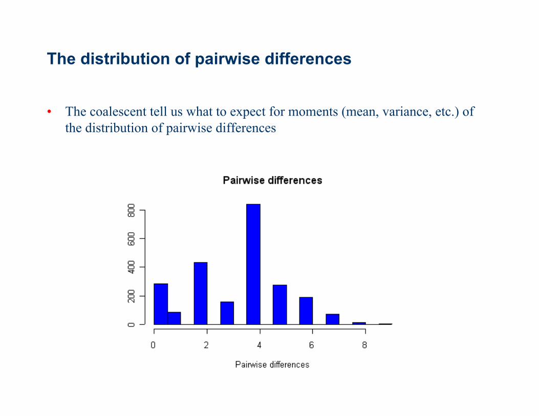
The distribution of pairwise differences

•  The coalescent tell us what to expect for moments (mean, variance, etc.) of the distribution of pairwise differences

Reconstructing the genealogy

•  We can also look for structure in the data by using simple clustering algorithms such as UPGMA –  Note that this is only going to ‘reconstruct’ the genealogy if there is no

recombination and lots of mutation

Single number summaries

•  There are several useful single-number summaries (summary statistics) of the data –  The number of segregating sites –  The average pairwise differences –  The number of singletons (sites at which only one individual differs from all

others) –  Neutrality statistics such as Tajima’s D and Fu and Li’s D*

Number of sequences = 69 Number of polymorphic sites = 33

Watterson's estimate of theta = 6.86919225575433 Average pairwise differences = 3.37595907928389 Number of singletons = 19 Tajima D statistic = -1.63320078310981 Fu and Li D statistic = -3.3243664840525

Statistical inference

Define model

Explore properties

Estimate parameters from data

Test goodness-of-fit

Refine model

rules parameters simulation

summary statistics graphical representation

moment methods likelihood

outliers heterogeneity

comparison of estimators

Issues

add parameters

Estimating parameters

•  The summaries of the data we have considered are good because they can be directly related to properties of the neutral coalescent model

•  For example, we know that the expected pairwise differences is just the parameter q, so the sample statistic is an unbiased estimate of the parameter

•  Likewise, the expected number of segregating sites is

•  So is also an unbiased estimate of q

∑−

=

=1

1

1][n

i iSE θ

∑−

=

1

1

1/n

i iS

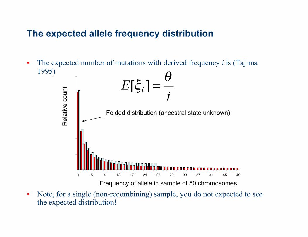
The expected allele frequency distribution

•  The expected number of mutations with derived frequency i is (Tajima 1995)

•  Note, for a single (non-recombining) sample, you do not expected to see the expected distribution!

1 5 9 13 17 21 25 29 33 37 41 45 49

Folded distribution (ancestral state unknown)

Frequency of allele in sample of 50 chromosomes

Rel

ativ

e co

unt

iE i

θξ =][

Other ways of estimating theta

•  We have considered a few moment estimators of theta. These compare statistics of the data to their expectations under the model

•  In general, moment methods are a quick but often poor way of estimating parameters because they throw away much of the information in the data

•  We can use more information by using likelihood methods. These calculate the probability of observing the data (or a summary of it) given the model. A natural choice of estimator is the maximum likelihood value

Data set n = 10 S = 14

1.12)ˆ(

9.5ˆ

=

=

π

π

θ

θ

Var 5.6)ˆ(

0.5ˆ

=

=

W

W

Var θ

θ

An example

•  Note, the estimator based on the average pairwise diversity has higher variance (and is not consistent), so it is generally a worse estimator

-3

-2

-1

00 2 4 6 8 10 12 14

Likelihood estimation of q

•  Using the recursion of Tavaré (1984) –  Number of segregating sites only

•  Using the full-likelihood method of Griffiths and Tavaré (1994) –  Implemented in GENETREE software

4.149.122.5ˆ

−==

Uθ

θ

Δ

2.129.127.4ˆ

−==

Uθ

S only

Full likelihood

Statistical inference

Define model

Explore properties

Estimate parameters from data

Test goodness-of-fit

Refine model

rules parameters simulation

summary statistics graphical representation

moment methods likelihood

outliers heterogeneity

comparison of estimators

Issues

add parameters

Testing the model

•  Given our parameter estimates, we want to ask how good the model is at describing the data

•  This is an example of a goodness of fit test. Generally, the idea is to take some other part of the data and ask how likely it is to see something as extreme as the observed value given the model (and the parameter estimates)

•  A widely used approach in population genetic is to compare estimators of theta –  Tajima D statistic compares estimators from the number of segregating sites

and pairwise diversity –  Fu and Li D* statistic compares estimates from the number of segregating sites

and the number of singletons

Tajima’s D test (1989)

•  Two estimators of theta –  Watterson’s estimate: number of segregating sites –  Average pairwise diversity: sensitive to intermediate allele frequencies

•  Negative values of D indicate an excess of rare mutations, positive values indicate an excess of intermediate frequency mutations

∑−

=

θ=

θ=π1

1

1][

][n

i iSE

E

)/Var(/

n

n

aSaSD

−π−π=

Difference normalised by s.d. like Z statistic

D > 0 D < 0 naS /<π naS />π

Fu and Li D test (1993)

•  Fu and Li (1993) D test

Expected number of external mutations

θη =][ eE

Without an outgroup, the test has to be adjusted (D*)

)Var( en

en

aSaSD

ηη−

−=

A general class of tests: Fu (1995)

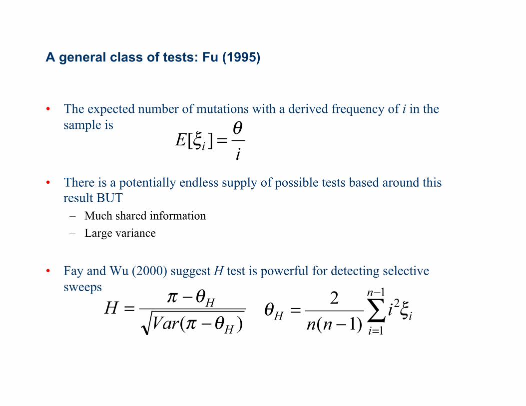
•  The expected number of mutations with a derived frequency of i in the sample is

•  There is a potentially endless supply of possible tests based around this result BUT –  Much shared information –  Large variance

•  Fay and Wu (2000) suggest H test is powerful for detecting selective sweeps

iE i

θξ =][

)( H

H

VarH

θπθπ−

−= ∑−

=−=

1

1

2

)1(2 n

iiH i

nnξθ

How do we spot an unusual observation?

•  We need to ask whether the statistic we have observed is unusual given the standard neutral model

•  We can either do this by looking up values in a table, or simulating data (preferable)

•  The basic idea is to simulate data under the null model lots (100s) of times and ask how striking an outlier the empirical observation is

More on testing the model

•  There are many ways in which we can look for departures from the assumed model (see also HKA test, McDonald-Kreitman test)

•  Different evolutionary forces that we have left out of the basic model will tend to have different effects on the data, so will be picked up by different ways of testing the null model

•  Watterson (1977)

“There is no single statistic which is best for testing the most general departures from neutrality”

Summary

•  Genetic data should be summarised in a manner that is informative about the underlying model parameters

•  There are a variety of estimators of the population mutation parameter, theta, most of which only use a small amount of information

•  Summary statistics can be used to test whether the coalescent provides an adequate description of the data

•  An important class of summary statistics are neutrality test statistics that compare different estimators of theta