Lecture Notes on Proofs as Programs - cs.cmu.edufp/courses/15816-s10/lectures/02-pap.pdf · Lecture...

Lecture Notes onProofs as Programs

15-816: Modal LogicFrank Pfenning

Lecture 2January 14, 2010

1 Introduction

In this lecture we investigate a computational interpretation of intuition-istic proofs and relate it to functional programming. On the propositionalfragment of logic this is called the Curry-Howard isomorphism [How80].From the very outset of the development of constructive logic and math-ematics, a central idea has been that proofs ought to represent construc-tions. The Curry-Howard isomorphism is only a particularly poignant andbeautiful realization of this idea. In a highly influential subsequent pa-per, Martin-Lof [ML80] developed it further into a more expressive calculuscalled type theory.

The computational interpretation of intuitionistic logic and type theoryunderlies many of the applications of intuitionistic modal logic in computerscience. In the context of this course it therefore important to gain a goodworking knowledge of the interpretation of proofs as programs.

2 Propositions as Types

In order to illustrate the relationship between proofs and programs we in-troduce a new judgment:

M : A M is a proof term for proposition A

We presuppose that A is a proposition when we write this judgment. Wewill also interpret M : A as “M is a program of type A”. These dual inter-

LECTURE NOTES JANUARY 14, 2010

L2.2 Proofs as Programs

pretations of the same judgment is the core of the Curry-Howard isomor-phism. We either think of M as a term that represents the proof of A true, orwe think of A as the type of the program M . As we discuss each connective,we give both readings of the rules to emphasize the analogy.

We intend that if M : A then A true. Conversely, if A true then M : A.But we want something more: every deduction of M : A should corre-spond to a deduction of A true with an identical structure and vice versa.In other words we annotate the inference rules of natural deduction withproof terms. The property above should then be obvious.

Conjunction. Constructively, we think of a proof of A ∧ B true as a pairof proofs: one for A true and one for B true.

M : A N : B

〈M,N〉 : A ∧B∧I

The elimination rules correspond to the projections from a pair to itsfirst and second elements.

M : A ∧B

π1 M : A∧EL

M : A ∧B

π2 M : B∧ER

Hence conjunction A ∧B corresponds to the product type A×B.

Truth. Constructively, we think of a proof of > true as a unit element thatcarries now information.

〈〉 : >>I

Hence > corresponds to the unit type 1 with one element. There is noelimination rule and hence no further proof term constructs for truth.

Implication. Constructively, we think of a proof of A⊃B true as a func-tion which transforms a proof of A true into a proof of B true.

In mathematics and many programming languages, we define a func-tion f of a variable x by writing f(x) = . . . where the right-hand side “. . .”depends on x. For example, we might write f(x) = x2 +x−1. In functionalprogramming, we can instead write f = λx. x2 +x−1, that is, we explicitlyform a functional object by λ-abstraction of a variable (x, in the example).


Proofs as Programs L2.3

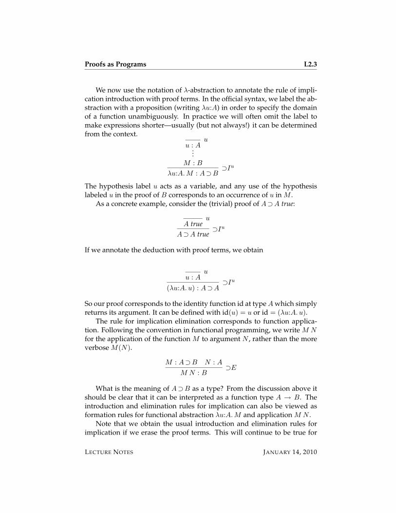
We now use the notation of λ-abstraction to annotate the rule of impli-cation introduction with proof terms. In the official syntax, we label the ab-straction with a proposition (writing λu:A) in order to specify the domainof a function unambiguously. In practice we will often omit the label tomake expressions shorter—usually (but not always!) it can be determinedfrom the context.

u : Au

...M : B

λu:A.M : A⊃B⊃Iu

The hypothesis label u acts as a variable, and any use of the hypothesislabeled u in the proof of B corresponds to an occurrence of u in M .

As a concrete example, consider the (trivial) proof of A⊃A true:

A trueu

A⊃A true⊃Iu

If we annotate the deduction with proof terms, we obtain

u : Au

(λu:A. u) : A⊃A⊃Iu

So our proof corresponds to the identity function id at type A which simplyreturns its argument. It can be defined with id(u) = u or id = (λu:A. u).

The rule for implication elimination corresponds to function applica-tion. Following the convention in functional programming, we write M Nfor the application of the function M to argument N , rather than the moreverbose M(N).

M : A⊃B N : A

M N : B⊃E

What is the meaning of A⊃B as a type? From the discussion above itshould be clear that it can be interpreted as a function type A → B. Theintroduction and elimination rules for implication can also be viewed asformation rules for functional abstraction λu:A.M and application M N .

Note that we obtain the usual introduction and elimination rules forimplication if we erase the proof terms. This will continue to be true for



all rules in the remainder of this section and is immediate evidence for thesoundness of the proof term calculus, that is, if M : A then A true.

As a second example we consider a proof of (A ∧B)⊃(B ∧A) true.

A ∧B trueu

B true∧ER

A ∧B trueu

A true∧EL

B ∧A true∧I

(A ∧B)⊃(B ∧A) true⊃Iu

When we annotate this derivation with proof terms, we obtain a functionwhich takes a pair 〈M,N〉 and returns the reverse pair 〈N,M〉.

u : A ∧Bu

π2 u : B∧ER

u : A ∧Bu

π1 u : A∧EL

〈π2 u, π1 u〉 : B ∧A∧I

(λu. 〈π2 u, π1 u〉) : (A ∧B)⊃(B ∧A)⊃Iu

Disjunction. Constructively, we think of a proof of A ∨ B true as eithera proof of A true or B true. Disjunction therefore corresponds to a disjointsum type A +B, and the two introduction rules correspond to the left andright injection into a sum type.

M : A

inlB M : A ∨B∨IL

N : B

inrA N : A ∨B∨IR

In the official syntax, we have annotated the injections inl and inr withpropositions B and A, again so that a (valid) proof term has an unambigu-ous type. In writing actual programs we usually omit this annotation. Theelimination rule corresponds to a case construct which discriminates be-tween a left and right injection into a sum types.

M : A ∨B

u : Au

...N : C

w : Bw

...O : C

case M of inl u ⇒ N | inr w ⇒ O : C∨Eu,w

Recall that the hypothesis labeled u is available only in the proof of thesecond premise and the hypothesis labeled w only in the proof of the thirdpremise. This means that the scope of the variable u is N , while the scopeof the variable w is O.



Falsehood. There is no introduction rule for falsehood (⊥). We can there-fore view it as the empty type 0. The corresponding elimination rule allowsa term of ⊥ to stand for an expression of any type when wrapped withabort. However, there is no computation rule for it, which means duringcomputation of a valid program we will never try to evaluate a term of theform abort M .

M : ⊥abortC M : C

⊥E

As before, the annotation C which disambiguates the type of abort M willoften be omitted.

This completes our assignment of proof terms to the logical inferencerules. Now we can interpret the interaction laws we introduced early asprogramming exercises. Consider the following distributivity law:

(L11a) (A⊃(B ∧ C))⊃(A⊃B) ∧ (A⊃C) trueInterpreted constructively, this assignment can be read as:

Write a function which, when given a function from A to pairsof type B ∧ C, returns two functions: one which maps A to Band one which maps A to C.

This is satisfied by the following function:

λu. 〈(λw. π1 (u w)), (λv. π2 (u v))〉

The following deduction provides the evidence:

u : A⊃(B ∧ C)u

w : Aw

u w : B ∧ C⊃E

π1 (u w) : B∧EL

λw. π1 (u w) : A⊃B⊃Iw

u : A⊃(B ∧ C)u

v : Av

u v : B ∧ C⊃E

π2 (u v) : C∧ER

λv. π2 (u v) : A⊃C⊃Iv

〈(λw. π1 (u w)), (λv. π2 (u v))〉 : (A⊃B) ∧ (A⊃C)∧I

λu. 〈(λw. π1 (u w)), (λv. π2 (u v))〉 : (A⊃(B ∧ C))⊃((A⊃B) ∧ (A⊃C))⊃Iu

Programs in constructive propositional logic are somewhat uninterest-ing in that they do not manipulate basic data types such as natural num-bers, integers, lists, trees, etc. These can be added, most elegantly in the



context of a type theory where we allow arbitrary inductive types. This ex-tension is somewhat orthogonal to the main aims of this course on modallogic so we will not treat it formally, but use it freely in examples.

To close this section we recall the guiding principles behind the assign-ment of proof terms to deductions.

1. For every deduction of A true there is a proof term M and deductionof M : A.

2. For every deduction of M : A there is a deduction of A true

3. The correspondence between proof terms M and deductions of A trueis a bijection.

3 Reduction

In the preceding section, we have introduced the assignment of proof termsto natural deductions. If proofs are programs then we need to explain howproofs are to be executed, and which results may be returned by a compu-tation.

We explain the operational interpretation of proofs in two steps. In thefirst step we introduce a judgment of reduction M =⇒R M ′, read “M reducesto M ′”. A computation then proceeds by a sequence of reductions M =⇒R

M1 =⇒R M2 . . ., according to a fixed strategy, until we reach a value whichis the result of the computation. In this section we cover reduction; we mayreturn to reduction strategies in a later lecture.

As in the development of propositional logic, we discuss each of theconnectives separately, taking care to make sure the explanations are inde-pendent. This means we can consider various sublanguages and we canlater extend our logic or programming language without invalidating theresults from this section. Furthermore, it greatly simplifies the analysis ofproperties of the reduction rules.

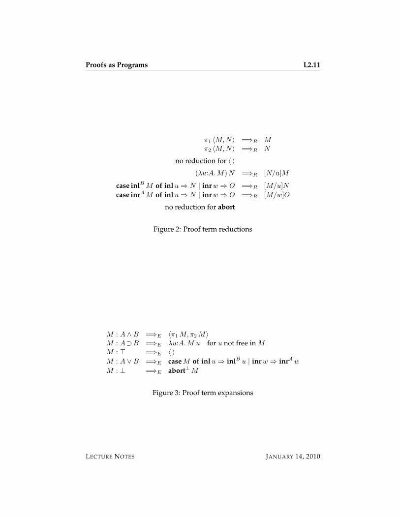
In general, we think of the proof terms corresponding to the introduc-tion rules as the constructors and the proof terms corresponding to the elim-ination rules as the destructors.

Conjunction. The constructor forms a pair, while the destructors are theleft and right projections. The reduction rules prescribe the actions of theprojections.



π1 〈M,N〉 =⇒R Mπ2 〈M,N〉 =⇒R N

Truth. The constructor just forms the unit element, 〈〉. Since there is nodestructor, there is no reduction rule.

Implication. The constructor forms a function by λ-abstraction, while thedestructor applies the function to an argument. In general, the applicationof a function to an argument is computed by substitution. As a simple ex-ample from mathematics, consider the following equivalent definitions

f(x) = x2 + x− 1 f = λx. x2 + x− 1

and the computation

f(3) = (λx. x2 + x− 1)(3) = [3/x](x2 + x− 1) = 32 + 3− 1 = 11

In the second step, we substitute 3 for occurrences of x in x2 + x − 1, thebody of the λ-expression. We write [3/x](x2 + x− 1) = 32 + 3− 1.

In general, the notation for the substitution of N for occurrences of u inM is [N/u]M . We therefore write the reduction rule as

(λu:A.M) N =⇒R [N/u]M

We have to be somewhat careful so that substitution behaves correctly. Inparticular, no variable in N should be bound in M in order to avoid conflict.We can always achieve this by renaming bound variables—an operationwhich clearly does not change the meaning of a proof term. A more formaldefinition is presented in Section 8.

Disjunction. The constructors inject into a sum types; the destructor dis-tinguishes cases. We need to use substitution again.

case inlB M of inl u ⇒ N | inr w ⇒ O =⇒R [M/u]Ncase inrA M of inl u ⇒ N | inr w ⇒ O =⇒R [M/w]O

Falsehood. Since there is no constructor for the empty type there is noreduction rule for falsehood.



This concludes the definition of the reduction judgment. In the next sec-tion we will prove some of its properties.

As an example we consider a simple program for the composition oftwo functions. It takes a pair of two functions, one from A to B and onefrom B to C and returns their composition which maps A directly to C.

comp : ((A⊃B) ∧ (B⊃C))⊃(A⊃C)

We transform the following implicit definition into our notation step-by-step:

comp 〈f, g〉 (w) = g(f(w))comp 〈f, g〉 = λw. g(f(w))

compu = λw. (π2 u) ((π1 u)(w))comp = λu. λw. (π2 u) ((π1 u) w)

The final definition represents a correct proof term, as witnessed by thefollowing deduction.

u : (A⊃B) ∧ (B⊃C)u

π2 u : B⊃C∧ER

u : (A⊃B) ∧ (B⊃C)u

π1 u : A⊃B∧EL

w : Aw

(π1 u) w : B⊃E

(π2 u) ((π1 u) w) : C⊃E

λw. (π2 u) ((π1 u) w) : A⊃C⊃Iw

(λu. λw. (π2 u) ((π1 u) w)) : ((A⊃B) ∧ (B⊃C))⊃(A⊃C)⊃Iu

We now verify that the composition of two identity functions reduces againto the identity function. First, we verify the typing of this application.

(λu. λw. (π2 u) ((π1 u) w)) 〈(λx. x), (λy. y)〉 : A⊃A

Now we show a possible sequence of reduction steps. This is by no meansuniquely determined.

(λu. λw. (π2 u) ((π1 u) w)) 〈(λx. x), (λy. y)〉=⇒R λw. (π2 〈(λx. x), (λy. y)〉) ((π1 〈(λx. x), (λy. y)〉) w)=⇒R λw. (λy. y) ((π1 〈(λx. x), (λy. y)〉) w)=⇒R λw. (λy. y) ((λx. x) w)=⇒R λw. (λy. y) w=⇒R λw. w



We see that we may need to apply reduction steps to subterms in orderto reduce a proof term to a form in which it can no longer be reduced. Wepostpone a more detailed discussion of this until we discuss the operationalsemantics in full.

4 Expansion

We saw in the previous section that proof reductions that witness localsoundness form the basis for the computational interpretation of proofs.Less relevant to computation are the local expansions. What they tell us,for example, is that if we need to return a pair from a function, we can al-ways construct it as 〈M,N〉 for some M and N . Another example wouldbe that whenever we need to return a function, we can always construct itas λu.M for some M .

We can derive what the local expansion must be by annotating the de-ductions witnessing local expansions from Lecture 1 with proof terms. Weleave this as an exercise to the reader. The left-hand side of each expan-sion has the form M : A, where M is an arbitrary term and A is a logicalconnective or constant applied to arbitrary propositions. On the right handside we have to apply a destructor to M and then reconstruct a term of theoriginal type. The resulting rules can be found in Figure 3.

5 Summary of Proof Terms

Judgments.M : A M is a proof term for proposition A, see Figure 1M =⇒R M ′ M reduces to M ′, see Figure 2M : A =⇒E M ′ M expands to M ′, see Figure 3

6 Hypothetical Judgments in Localized Form

The isomorphism between proofs and programs seems obvious, but it isnonetheless a useful exercise to rigorously prove this relationship as a prop-erty of the deductive systems we have developed. When we proceed to acertain level of formality in our analysis, it is beneficial to write hypotheti-


http://www.cs.cmu.edu/~fp/courses/15816-s10/lectures/01-judgments.pdf


Constructors Destructors

M : A N : B

〈M,N〉 : A ∧B∧I

M : A ∧B

π1 M : A∧EL

M : A ∧B

π2 M : B∧ER

〈〉 : >>I

no destructor for >

u : Au

...M : B

λu:A.M : A⊃B⊃Iu

M : A⊃B N : A

M N : B⊃E

M : A

inlB M : A ∨B∨IL

N : B

inrA N : A ∨B∨IR

M : A ∨B

u : Au

...N : C

w : Bw

...O : C

case M of inl u ⇒ N | inr w ⇒ O : C∨Eu,w

no constructor for ⊥M : ⊥

abortC M : C⊥E

Figure 1: Proof term assignment for natural deduction



π1 〈M,N〉 =⇒R Mπ2 〈M,N〉 =⇒R N

no reduction for 〈〉

(λu:A.M) N =⇒R [N/u]M

case inlB M of inl u ⇒ N | inr w ⇒ O =⇒R [M/u]Ncase inrA M of inl u ⇒ N | inr w ⇒ O =⇒R [M/w]O

no reduction for abort

Figure 2: Proof term reductions

M : A ∧B =⇒E 〈π1 M,π2 M〉M : A⊃B =⇒E λu:A.M u for u not free in MM : > =⇒E 〈〉M : A ∨B =⇒E case M of inl u ⇒ inlB u | inr w ⇒ inrA w

M : ⊥ =⇒E abort⊥ M

Figure 3: Proof term expansions



cal judgmentsJ1 · · · Jn...

J

in their localized formJ1, . . . , Jn ` J.

When we try to recast the two-dimensional rules, however, some ambigui-ties in the two-dimensional notation need to be clarified.

The first ambiguity can be seen from considering the question of howmany verifications of P ⊃P ⊃P there are. Clearly, there should be two: oneusing the first assumption and one using the second assumption. Indeed,after a few steps we arrive at the following situation

P↓u

P↓w

...P↑

P ⊃P↑⊃Iw

P ⊃P ⊃P↑⊃Iu

Now we can use the ↓↑ rule with the hypothesis labeled u or the hypothesislabeled w. If we look at the hypothetical judgment that we still have toprove and write it as

P↓, P↓ ` P↑

then it is not clear if or how we should distinguish the two occurrences ofP↓. We can do this by labeling them in the local notation for hypotheticaljudgments. But we have already gone through this exercise before, whenintroducing proof terms! We therefore forego a general analysis of how todisambiguate hypothetical judgments and just work with proof terms.

The localized version of this judgment has the form

x1:A1, . . . , xn:An︸︷︷︸Γ

` M : C

where we abbreviate the collection of assumptions by Γ. We often refer toΓ as the context for the judgment M : C. Following general convention andtheir use in the proof term M , we now use variables x, y, z for labels ofhypotheses. The turnstile ‘`’ is the universal symbol indicating a hypothet-ical judgment, with the hypotheses on the left and the conclusion on the



right. Since the goal is to have an unambiguous representation of proofs,we require all variables x1, . . . , xn to be distinct. Of course, some of thepropositions A1, . . . , An may be the same, as they would be in the proofof A⊃A⊃A. We write ‘·’ for an empty collection of hypotheses when wewant to emphasize that there are no assumptions.

The definition of the notion of hypothetical judgment was as an incom-plete proof. This means we can always substitute an actual proof for themissing one. That is, any time we use the turnstile (`) symbol, we meanthat it must satisfy the following principle, now written in localized form.

Substitution, v.1: If Γ1, x:A,Γ3 ` N : C and Γ2 ` M : A thenΓ1,Γ2,Γ3 ` [M/x]N : C.

A second important principle which is implicit in the two-dimensionalnotation for hypothetical judgments is that hypotheses need not be used.For example, in the proof

x:A, y:B ` x : Ax

x:A ` λy. x : B⊃A⊃Iy

· ` (λx. λy. x) : A⊃B⊃A⊃Ix

we find the judgment x:A, y:B ` x : A where y is not used. In two-dimensional notation, this would just be written as

x : Ax

which would just be x:A ` x : A since there is no natural place to displayy:B. Moreover, it might be used later in the context of a larger proof whereother assumptions become available, which would also not be shown.

What emerges is a general principle of weakening.

Weakening: If Γ1,Γ2 ` N : C then Γ1, x:A,Γ2 ` N : C.

It is implicit here that x does not already occur in Γ1 and Γ2, which is nec-essary so that the new context Γ1, x:A,Γ2 is well-formed.

We also have the principle of contraction, whose justification can be seenby going back to the original definition of hypothetical judgments. Doesthe hypothetical proof

A ∧B trueB true

∧ERA ∧B true

A true∧EL

B ∧A true∧I



correspond to A∧B true ` B∧A true or A∧B true, A∧B true ` B∧A true?Depending on the situation in which we use this, both are possible. Forexample, during the proof of A ∧ B⊃B ∧ A we would be taking the firstinterpretation, while the second might come out of a proof of A ∧ B⊃A ∧B⊃B ∧A.

In general, we can always contract two assumptions by identifying thevariables that label them: we simply replace any use by either x or y by z.

Contraction: If Γ1, x:A,Γ2, y:A,Γ3 ` N : C then Γ1, z:A,Γ2,Γ3 `[z/x, z/y]N : C.

Again, it is implicit that z be chosen distinct from the variables in Γ1,Γ2,Γ3.Finally, we may note that the order of the hypotheses in Γ is irrelevant.

Exchange: If Γ1, x:A, y:B,Γ2 ` N : C then Γ1, y:B, x:A,Γ2 ` N :C.

We will have occasion to consider systems where some of the principlesof weakening, contraction, or exchange are violated. For example, in linearlogic, weakening and contraction are restricted to specific circumstances,in ordered logic exchange is also repudiated. Also, in dependent type theorywe have dependencies between assumptions so that some cannot be ex-changed, even if weakening and contraction do hold.

The one invariant, however, is the substitution principle since we viewis as the defining property of hypothetical judgments.However, even thesubstitution principle has different forms, depending on how we employ it.Consider the local reduction of (λx:A.N) M =⇒R [M/x]N . We would liketo demonstrate that if the left-hand side is a valid proof term, then the right-hand side is as well. This property is called subject reduction. It verifies thatthe local reduction, when written on proof terms, really is a proper localreduction when considered as an operation on proofs. By inspection ofthe rules (which we will develop below), we see that if Γ ` (λx:A.N) M :C then Γ, x:A ` N : C and Γ ` M : A. Now the assumptions of thesubstitution principle above do not quite apply, so it is convenient to havean alternative formulation that matches this particular use.

Substitution, v.2: If Γ1, x:A,Γ2 ` N : C and Γ1 ` M : A thenΓ1,Γ2 ` [M/x]N : C.

This now matches the property we need for Γ2 = (·). Under the rightcircumstances, the two versions of the substitution principle coincide (seeExercise 5).



7 Natural Deduction in Localized Form

We now revisit the rules for natural deduction, using the local form of hy-pothetical judgments, thereby making the contexts of each judgment ex-plicit. We read these rules from the conclusion to the premises. For ex-ample (eliding proof terms), in order to prove Γ ` A ∧ B true we have toprove Γ ` A and Γ ` B, making all current assumptions Γ available forboth subproofs. The rules in this form are summarized in Figure 4. Thereis an alternative possibility, reading the rules from premises to conclusionwhich is pursued in Exercise 6.

The rules ⊃I and ∨E that introduce new hypotheses, are now usuallyno longer labeled, because we track the assumption and its name locally,in the context. We have to be careful to maintain the assumption thatall variables in a context are distinct. For example, would we consider` λx:A. λx:B. x : A⊃B⊃B to be a correct judgment? It appears we mightbe stuck at the point

x:A ` λx:B. x : B⊃B

but we are not, because we can always silently rename bound variables. Inthis case, this is indistinguishable from

x:A ` λy:B. y : B⊃B

which is now easily checked.We also see that we acquired one new rule when writing the judgment

in its localized form which makes the use of a hypothesis explicit:

Γ1, x:A,Γ2 ` x : Ahyp

which could also be written as

x:A ∈ ΓΓ ` x : A

hyp

This rule is not connected to any particular logical connective, but is de-rived from the nature of the hypothetical judgment. We often refer to suchrules as judgmental rules because they are concerned with judgments ratherthan any specific propositions.



Γ1, x:A,Γ2 ` x : Ahyp

Constructors Destructors

Γ ` M : A Γ ` N : B

Γ ` 〈M,N〉 : A ∧B∧I

Γ ` M : A ∧B

Γ ` π1 M : A∧EL

Γ ` M : A ∧B

Γ ` π2 M : B∧ER

Γ ` 〈〉 : >>I

no destructor for >

Γ, x:A ` M : B

Γ ` λx:A.M : A⊃B⊃I

Γ ` M : A⊃B Γ ` N : A

Γ ` M N : B⊃E

Γ ` M : A

Γ ` inlB M : A ∨B∨IL

Γ ` N : B

Γ ` inrA N : A ∨B∨IR

Γ ` M : A ∨B Γ, x:A ` N : C Γ, y:B ` O : C

Γ ` case M of inl x ⇒ N | inr y ⇒ O : C∨E

no constructor for ⊥Γ ` M : ⊥

Γ ` abortC M : C⊥E

Figure 4: Proof term assignment for natural deduction with contexts



8 Subject Reduction

We would like to prove that local reduction, as expressed on proof terms,preserves types. In some sense the idea is already contained in the displayof local reduction on proofs themselves, since the judgment A true remainsunchanged. Now we reexamine this in a more formal setting, where proofterms are explicit and hypotheses are listed explicitly as part of hypotheti-cal judgments.

The reduction for implication, (λx:A.N) N =⇒R [M/x]N , suggests thatwe will first need a property of substitution, already stated in Section 6.We take for granted the property of weakening, which just adds an unusedhypothesis but otherwise leaves the proof unchanged. Before we undertakethe proof, we should formally define the substitution as an operation onterms. For that we define the notion of a free variable in a term. We say x isfree in M if x occurs in M outside the scope of a binder for x. Note that ifΓ ` M : A then any free variable in M must be declared in Γ. The point ofthe terminology is to be able to define certain operations without requiringterms to be a priori well-typed or carrying around explicit contexts at alltimes.

[M/x]x = M[M/x]y = y for x 6= y

[M/x](〈N1, N2〉) = ([M/x]N1) ([M/x]N2)[M/x](π1 N) = π1 ([M/x]N)[M/x](π2 N) = π2 ([M/x]N)

[M/x](〈〉) = 〈〉

[M/x](λy:A.N) = λy:A. [M/x]N provided x 6= y and y not free in M[M/x](N1 N2) = ([M/x]N1) ([M/x]N2)

[M/x](inlB N) = inlB ([M/x]N)[M/x](inrA N) = inrA ([M/x]N)[M/x](case N1 of inl y ⇒ N2 | inr z ⇒ N3)

= case ([M/x]N1) of inl y ⇒ ([M/x]N2) | inr z ⇒ ([M/x]N3)provided x 6= y, x 6= zand y and z not free in M

[M/x](abortC N) = abortC ([M/x]N)

We call the definition of substitution compositional because it pushes the



substitution through to all subterms and recomposes the results with thesame constructor or destructor. This is a key observation, because it tellsus that the definition is modular: if we add a new logical connective oroperator to the language, substitution is always extended compositionally.This should have been clear from the beginning, given the intuitive pictureof replacing an unproven assumption in a proof with an actualy proof.

We also say that the definition of [M/x]N is by induction on the struc-ture of N , because on the right-hand side the substitution is always appliedto subterms. Since we also have a clause for every possible case, this guar-antees that substitution is always defined. To see this we just have to ob-serve that the provisos on the clauses that bind variables (λ and case) canalways be satisfied by renaming, which we do silently.

Theorem 1 (Substitution) If Γ ` M : A and Γ, x:A,Γ′ ` N : C then Γ,Γ′ `[M/x]N : C

Proof: By induction on N . This is suggested by the fact that the substitu-tion operation itself is defined by induction on N . We show a few repre-sentative cases.

Case: N = x.

Γ, x:A,Γ′ ` x : C GivenA = C By inversion, since var. decls. are uniqueΓ ` M : A GivenΓ,Γ′ ` M : A By weakeningΓ,Γ′ ` [M/x]x : A Since [M/x]x = MΓ,Γ′ ` [M/x]x : C Since A = C

Case: N = y for y 6= x.

Γ ` M : A GivenΓ, x:A,Γ′ ` y : C Giveny:C ∈ (Γ,Γ′) By inversion and y 6= xΓ,Γ′ ` y : C By rule hyp

Case: N = N1 N2.

Γ, x:A,Γ′ ` N1 N2 : C GivenΓ, x:A,Γ′ ` N1 : C2⊃C andΓ, x:A,Γ′ ` N2 : C2 By inversion



Γ,Γ′ ` [M/x]N1 : C2⊃C By i.h. on N1

Γ,Γ′ ` [M/x]N2 : C2 By i.h. on N2

Γ,Γ′ ` ([M/x]N1) ([M/x]N2) : C By rule ⊃EΓ,Γ′ ` [M/x](N1 N2) : C By defn. of [M/x](N1 N2)

Case: N = (λy. N1).

Γ, x:A,Γ′ ` (λy. N1) : C GivenΓ, x:A,Γ′, y:C2 ` N1 : C1 andC = C2⊃C1 for some C1, C2 By inversionΓ,Γ′, y:C2 ` [M/x]N1 : C1 by i.h. on N1

Γ,Γ′ ` λy:C2. [M/x]N1 : C1 By rule ⊃IΓ,Γ′ ` [M/x](λy:C2. N1) : C1 By definition of [M/x](λy:C2. N1)

In this last case worth verifying that the provisos in the definition of[M/x](λy:C2. N1) are satisfied to see that it is equal to λy:C2. [M/x]N1.When we applied inversion, we formed Γ, x:A,Γ′, y:C2, possibly ap-plying some implicit renaming to make sure y was different from xand any variable in Γ and Γ′. Since the free variables of M are con-tained in Γ, the proviso must be satisfied.

�

Now we return to subject reduction proper. We only prove it for a top-level (local) reduction. It should be clear by a simple additional argumentthat if the reduction takes place anywhere inside a term, the type of theoverall term also is preserved.

Theorem 2 (Subject Reduction) If Γ ` M : A and M =⇒R M ′ then Γ `M ′ : A.

Proof: By cases on M =⇒R M ′, using inversion on the typing derivationin each case. We show a few cases.

Case: π1〈M1,M2〉 =⇒R M1.

Γ ` π1〈M1,M2〉 : A GivenΓ ` 〈M1,M2〉 : A ∧B for some B By inversionΓ ` M1 : A and Γ ` M2 : B By inversion

Case: π2〈M1,M2〉 =⇒R M2. Symmetric to the previous case.



Case: (λx:A2.M1) M2 =⇒R [M2/x]M1.

Γ ` (λx:A2.M1) M2 : A GivenΓ ` λx:A2.M1 : A2⊃A andΓ ` M2 : A2 By inversionΓ, x:A2 ` M1 : A By inversionΓ ` [M2/x]M1 : A By substitution (Theorem 1)

�

An analogous theorem holds for local expansion; see Exercise 11.The material so far is rather abstract, in that it does not commit to

whether we are primarily interested in logical reasoning or programming.If we want to take this further, the two views which are perfectly unifiedat this point, will start to drift apart. From the logical point of view, weneed to investigate how to prove global soundness and completeness asintroduced at the end of Lecture 1.

From a programming language perspective, we are interested in defin-ing an operational semantics which applies local reductions in a preciselyspecified manner to subterms. With respect to such a semantics we canprove progress (either we have a value, or we can perform a reduction step)on well-typed program and totality (all well-typed programs have a value).Some progress has been made to understand the choices that still remain inthe definition of the operational semantics from a logical point of view, butin the end the interpretation of proofs as programs remains as an impor-tant guide to the design of the type structure of a language, but is not thefinal word. We will often return to these questions of the operational se-mantics, because much of our investigation of various intuitionistic modallogics and their computational interpretations will be at this interface.


http://www.cs.cmu.edu/~fp/courses/15816-s10/lectures/01-judgments.pdf


Exercises

Exercise 1 Write proof terms for each direction of the interaction laws (L13),(L19), and (L20). Abuse the type inference engine of your favorite functional pro-gramming language (ML, Haskell, . . .) to check the correctness of your proof terms.

Exercise 2 Two types A and B are isomorphic if there are functions M : A⊃Band N : B⊃A such that their compositions λx:A.N (M x) : A⊃A and λy:B.M (N y) :B⊃B are both identity functions.

For example, A ∧B and B ∧A are isomorphic, because

λy:A ∧B. 〈π2 y, π1 y〉 : (A ∧B)⊃(B ∧A)

andλz:B ∧A. 〈π2 y, π1 y〉 : (B ∧A)⊃(A ∧B)

andλx. (λy. 〈π2 y, π1 y〉) ((λz. 〈π2 z, π1 z〉) x)≡ λx. (λy. 〈π2 y, π1 y〉) 〈π2 x, π1 x〉≡ λx. 〈π2 〈π2 x, π1 x〉, π1 〈π2 x, π1 x〉〉≡ λx. 〈π1 x, π1 〈π2 x, π1 x〉〉≡ λx. 〈π1 x, π2 x〉≡ λx. x

and symmetrically for the other direction. Here we used the congruence (≡) gener-ated by reductions and expansions, used in either direction and applied to arbitrarysubterms.

Check which among, (L13), (L19), and (L20) are type isomorphisms, usingonly local reductions and expansions, in either direction, on any subterm, in orderto show that the compositions are the identity.

For those that fail, is it the case that the types are simply not isomorphic, ordoes the failure suggest additional equivalences between proof terms that might bejustified?

Exercise 3 Proceed as in Exercises 1 and 2, but for laws (L4) and (L6).

Exercise 4 We could try to add a second rule for uses of falsehood, namely

⊥↓C↓

⊥E

Give arguments for an against such a rule, using examples and counterexamples.



Exercise 5 Carefully state the relationship between the two versions of the substi-tution principle and prove that it is satisfied.

Exercise 6 We can write a system with localized hypotheses where each rule isnaturally read from the premises to the conclusion and only records hypothesesthat are actually used. For example, we can rewrite ∧I and hyp as

Γ1 ` M : A Γ2 ` N : B

Γ1,Γ2 ` 〈M,N〉 : A ∧B∧I

x:A ` x : Ahyp

(i) Complete the system of rules.

(ii) State the precise relationship with the system in Figure 4.

(iii) Prove that relationship.

Exercise 7 Show the cases concerning pairs in the proof of the substitution prop-erty (Theorem 1).

Exercise 8 Show the cases concerning disjunction in the proof of the substitutionproperty (Theorem 1).

Exercise 9 As pragmatists, we can define a new connective A⊗B by the followingelimination rule.

A⊗B true

A trueu

B truew

...C true

C true⊗Eu,w

(i) Write down corresponding introduction rules.

(ii) Show local reductions to verify local soundness.

(iii) Show local expansion to verify local completeness.

(iv) Define verifications and uses of A⊗B.

(v) Devise a notation for proof terms and show versions of the rules with localhypotheses and proof terms.

(vi) Reiterate local reduction and expansions on proof terms.

(vii) Extend the definition of substitution to include the new terms.



(viii) Extend the proof of the substitution property to encompass the new terms.

(ix) Show the new cases in subject reduction.

(x) Can we express A ⊗ B as an equivalent proposition in variables A and Busing only conjunction, implication, disjunction, truth, and falsehood? Ifso, prove the logical equivalence. If not, explain why not.

(xi) Can you relate the proof terms for A⊗B to constructs in existing functionallanguages such as Haskell or ML?

Exercise 10 As verificationists, we can define a new connective A ∧L B with thefollowing introduction rule.

A true

A trueu

...B true

A ∧L B true∧LIu

(i) Write down the corresponding elimination rules.

(ii)–(xi) as in Exercise 9, where in part (x), try to define A ∧L B in terms of theexisting connectives.

Exercise 11 Prove subject expansion: If Γ ` M : A and M : A =⇒E M ′ thenΓ ` M ′ : A.



References

[How80] W. A. Howard. The formulae-as-types notion of construction.In J. P. Seldin and J. R. Hindley, editors, To H. B. Curry: Essayson Combinatory Logic, Lambda Calculus and Formalism, pages 479–490. Academic Press, 1980. Hitherto unpublished note of 1969,rearranged, corrected, and annotated by Howard.

[ML80] Per Martin-Lof. Constructive mathematics and computer pro-gramming. In Logic, Methodology and Philosophy of Science VI,pages 153–175. North-Holland, 1980.


Lecture Notes on Proofs as Programs - cs.cmu.edufp/courses/15816-s10/lectures/02-pap.pdf · Lecture...

Documents

Transcript of Lecture Notes on Proofs as Programs - cs.cmu.edufp/courses/15816-s10/lectures/02-pap.pdf · Lecture...