LECTURE NOTES

ON

DIGITAL COMMUNICATIONS

Fig. 1.1: Block diagram of Communication System

The three basic elements of every communication systems areTransmitter,Receiver andChannel.The Overall purpose of this system is to transfer information from one point (called Source)

UNIT – I

ELEMENTS OF DIGITAL COMMUNICATION SYSTEMS

The purpose of a Communication System is to transport an information bearing signal from a

source to a user destination via a communication channel.

MODEL OF A COMMUNICATION SYSTEM

to another point, the user destination.

The message produced by a source, normally, is not electrical. Hence an input transducer is

used for converting the message to a time – varying electrical quantity called message signal.

Similarly, at the destination point, another transducer converts the electrical waveform to the

appropriate message.

The transmitter is located at one point in space, the receiver is located at some other point

separate from the transmitter, and the channel is the medium that provides the electrical

connection between them.

The purpose of the transmitter is to transform the message signal produced by the source of

information into a form suitable for transmission over the channel.

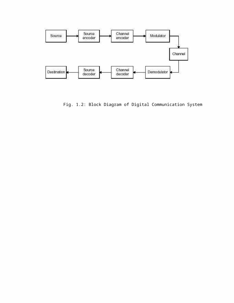
ELEMENTS OF DIGITAL COMMUNICATION SYSTEMS:The figure 1.2 shows the functional elements of a digital communication system. Source of Information:1. Analog Information Sources.2. Digital Information Sources.Analog Information Sources → Microphone actuated by a speech, TV Camera scanning a scene, continuous amplitude signals.Digital Information Sources → These are teletype or the numerical output of computer which consists of a sequence of discrete symbols or letters.An Analog information is transformed into a discrete information through the process of sampling and quantizing.Digital Communication System

The received signal is normally corrupted version of the transmitted signal, which is due to

channel imperfections, noise and interference from other sources.The receiver has the task of

operating on the received signal so as to reconstruct a recognizable form of the original

message signal and to deliver it to the user destination.

Communication Systems are divided into 3 categories:

1. Analog Communication Systems are designed to transmit analog information using

analog modulation methods.

2. Digital Communication Systems are designed for transmitting digital information using

digital modulation schemes, and

3. Hybrid Systems that use digital modulation schemes for transmitting sampled and

quantized values of an analog message signal.

Fig. 1.2: Block Diagram of Digital Communication System

words is quite simple, but the decoder for a system using variable – length code words will be very complex.Aim of the source coding is to remove the redundancy in the transmitting information, so that bandwidth required for transmission is minimized. Based on the probability of the symbol code word is assigned. Higher the probability, shorter is the codeword.Ex: Huffman coding.CHANNEL ENCODER / DECODER:Error control is accomplished by the channel coding operation that consists of systematically adding extra bits to the output of the source coder.These extra bits do not convey any information but helps the receiver to detect and /

SOURCE ENCODER / DECODER:The Source encoder ( or Source coder) converts the input i.e. symbol sequence into a

binary sequence of 0s and 1s by assigning code words to the symbols in the input

sequence. For eg. :-If a source set is having hundred symbols, then the number of

bits used to represent each symbol will be 7 because 27=128 unique combinations are

available. The important parameters of a source encoder are block size, code

word lengths, average data rate and theefficiency of the coder (i.e. Actual output

data rate compared to the minimum achievable rate)

At the receiver, the source decoder converts the binary output of the channel

decoder into a symbol sequence. The decoder for a system using fixed – length code

or correct some of the errors in the information bearing bits. There are two methods

of channel coding:

1. Block Coding: The encoder takes a block of k information bits from

the source encoder and adds r error control bits, where r is dependent on k and

error control capabilities desired.

2. Convolution Coding: The information bearing message stream is encoded in

a continuous fashion by continuously interleaving information bits and error

control bits.

spectrumoftransmittedsignalwithchannel characteristics, to provide thecapability to multiplex many signals.

DEMODULATOR:The extraction of the message from the information bearing waveform produced by the modulation is accomplished by the demodulator. The output of the demodulatoris bit stream. The important parameter is the method of demodulation.

CHANNEL:The Channel provides the electrical connection between the source and destination.

The Channel decoder recovers the information bearing bits from the coded binary

stream. Error detection and possible correction is also performed by the channel

decoder.

The important parameters of coder / decoder are: Method of coding, efficiency,

error control capabilities and complexity of the circuit.

MODULATOR:

The Modulator converts the input bit stream into an electrical waveform

suitable for transmission over the communication channel. Modulator can be

effectively used to minimize the effects of channel noise, tomatch the frequency

The different channels are: Pair of wires, Coaxial cable, Optical fibre, Radio

channel, Satellite channel or combination of any of these.

The communication channels have only finite Bandwidth, non-ideal frequency

response, the signal often suffers amplitude and phase distortion as it travels over the

channel. Also, the signal power decreases due to the attenuation of the channel.

The signal iscorrupted by unwanted, unpredictable electrical signals referred to as

noise.

•Transmission Rate (measured in bits per second): This is a measure of the number of bits that can be transmitted over the communication channel per unit time.Bandwidth Requirements (measured in Hz): This is a measure of the spectrum that the communication system requires to transmit the information at the desired transmission rate.Error probability (measured in percentages): This represents the percentage of bits that are in error relative to the overall number of bits that are transmitted by the communication system.Transmission Power (or Bit Energy) (measured in Watts (or Jules/bit)): This

represents the amount of power of the transmitted signal that would be required toachieve a particular desired error probability.

The important parameters of the channel are Signal to Noise power Ratio(SNR),

usable bandwidth, amplitude and phase response and the statistical properties of

noise.

Certain Issues in Digital Transmission

Sometimes, a comparison between two digital transmission systems is needed. There

are many parameters that can be used to compare between digital transmission

systems, but some of the most important parameters of a digital transmission system

are:

• System Complexity (measured in cost of building or operating the system):

This represents that amount of money that a manufacturer will have to spend to build

the system and the amount of money that a user will have to pay to use the system.

The performance of a digital transmission system is a function of the

following factors:

1. Amount of energy in each digital bit (or pulse): Generally, the more energy a

digital bit (or pulse) has, the better the performance that the system will have.

either transmit at a higher transmission bit rate while keeping the same probability of bit error, or we can transmit at the same transmission bit rate but reduce the probability of bit error. Generally, the larger the bandwidth allocated to acommunication system, the better the performance it will have.

Advantages of Digital CommunicationThe effect of distortion, noise and interference is less in a digital communication system. This is because the disturbance must be large enough to change the pulse from one state to the other.Regenerative repeaters can be used at fixed distance along the link, to identify andregenerate a pulse before it is degraded to an ambiguous state.

2. The distance between the transmitter and receiver: Because energy is spread

or attenuated as it travels over the channel and more noise is added due to the

existence of more noise sources over long channels, generally the longer the path that

the digital transmitted signal has to travel, the worse the performance that the system

will have. However, you do not always have control over the distance between the

transmitted and receiver.

3. Amount of noise that is added to the signal: Certainly, the less the noise that

is added to the transmitted signal, the better the performance of the communication

system. We usually have limited control over the added noise.

4. Bandwidth of the transmission channel: By using larger bandwidth, we can

3. Digital circuits are more reliable and cheaper compared to analog circuits.

4. The Hardware implementation is more flexible than analog hardware because of

the use of microprocessors, VLSI chips etc.

5. Signal processing functions like encryption, compression can be employed to

maintain the secrecy of the information.

6. Error detecting and Error correcting codes improve the system performance by

reducing the probability of error.

7. Combining digital signals using TDM is simpler than combining analog signals

using FDM. The different types of signals such as data, telephone, TV can be treated

as identical signals in transmission and switching in a digital communication system.

characteristics of the channel. The two main characteristics of the channel are BANDWIDTH and POWER. In addition the other characteristics are whether the channel is linear or nonlinear, and how free the channel is free from the externalinterference.

Five channels are considered in the digital communication, namely: telephone channels, coaxial cables, optical fibers, microwave radio, and satellite channels.Telephone channel: It is designed to provide voice grade communication. Also good for data communication over long distances. The channel has a band-pass characteristic occupying the frequency range 300Hz to 3400hz, a high SNR ofabout 30db, and approximately linear response.

8. We can avoid signal jamming using spread spectrum

technique. Disadvantages of Digital Communication:

1. Large System Bandwidth:- Digital transmission requires a large system

bandwidth to communicate the same information in a digital format as compared to

analog format.

2. System Synchronization:- Digital detection requires system synchronization

whereas the analog signals generally have no such requirement.

Channels for Digital Communications

The modulation and coding used in a digital communication system depend on the

For the transmission of voice signals the channel provides flat amplitude

response. But for thetransmission of data and image transmissions, since the phase

delay variations are important an equalizer is used to maintain the flat amplitude

response and a linear phase response over the required frequency band.

Transmission rates upto16.8 kilobits per second have been achieved over the

telephone lines.

Coaxial Cable: The coaxial cable consists of a single wire conductor centered

inside an outer conductor, which is insulated from each other by a dielectric. The

main advantages of the coaxial cable are wide bandwidth and low external

Compared to coaxial cables, optical fibers are smaller in size and they offer higher transmission bandwidths and longer repeater separations.Microwave radio: A microwave radio, operating on the line-of-sight link, consists basically of a transmitter and a receiver that are equipped with antennas. The antennas are placed on towers at sufficient height to have the transmitter and receiver in line-of-sight of each other. The operating frequencies range from 1 to30 GHz.

Under normal atmospheric conditions, a microwave radio channel is veryreliable and provides path for high-speed digital transmission.But during meteorological variations, a severe degradation occurs in the system performance.

interference. But closely spaced repeaters are required. With repeaters spaced at 1km

intervals the data rates of 274 megabits per second have been achieved.

Optical Fibers: An optical fiber consists of a very fine inner core made of silica

glass, surrounded by a concentric layer called cladding that is also made of glass. The

refractive index of the glass in the core is slightly higher than refractive index of the

glass in the cladding. Hence if a ray of light is launched into an optical fiber at the

right oblique acceptance angle, it is continually refracted into the core by the

cladding. That means the difference between the refractive indices of the core and

cladding helps guide the propagation of the ray of light inside the core of the fiber

from one end to the other.

Satellite Channel: A Satellite channel consists of a satellite in geostationary orbit, an

uplink from ground station, and a down link to another ground station. Both link

operate at microwave frequencies, with uplink the uplink frequency higher than the

down link frequency. In general, Satellite can be viewed as repeater in the sky. It

permits communication over long distances at higher bandwidths and relatively low

cost.

Bandwidth:

megabit per second.

SamplingA message signal may originate from a digital or analog source. If the message signal is analog in nature, then it has to be converted into digital form before it can transmitted by digital means. The process by which the continuous-time signal is converted into a discrete–time signal is called Sampling.Sampling operation is performed in accordance with the sampling theorem.

Bandwidth is simply a measure of frequency range. The range of frequencies

contained in a composite signal is its bandwidth. The bandwidth is normally a

difference between two numbers. For example, if a composite signal contains

frequencies between 1000 and 5000, its bandwidth is 5000 - or 4000. If a range of

2.40 GHz to 2.48 GHz is used by a device, then the bandwidth would be 0.08 GHz

(or more commonly stated as 80MHz).It is easy to see that the bandwidth we define

here is closely related to the amount of data you can transmit within it - the more

room in frequency space, the more data you can fit in at a given moment. The term

bandwidth is often used for something we should rather call a data rate, as in “my

Internet connection has 1 Mbps of bandwidth”, meaning it can transmit data at 1

Sampling Theorem for Lowpass Signals

Part - I If a signal x(t) does not contain any frequency component beyond W Hz, then

the signal is completely described by its instantaneous uniform samples with

sampling interval (or period ) of Ts< 1/(2W) sec.

Part – II The signal x(t) can be accurately reconstructed (recovered) from the set of

uniform instantaneous samples by passing the samples sequentially through an ideal

(brick-wall) lowpass filter with bandwidth B, where W ≤ B < fs – W and fs = 1/(Ts).

using the theory of instantaneous sampling, as a fairly close approximation ofinstantaneous sampling is sufficient for most practical systems. To contain our discussion on Nyquist’s theorems, we will introduce some mathematical expressions.

If x(t) represents a continuous-time signal, the equivalent set of instantaneousuniform samples {x(nTs)} may be represented as,

{x(nTs)}≡ xs(t) = Σ x(t).δ(t- nTs)(1)where x(nTs) = x(t) t =nTs , δ(t) is a unit pulse singularity function and ‘n’ is an integer

As the samples are generated at equal (same) interval (Ts) of time, the process of

sampling is called uniform sampling. Uniform sampling, as compared to any non-

uniform sampling, is more extensively used in time-invariant systems as the theory of

uniform sampling (either instantaneous or otherwise) is well developed and the

techniques are easier to implement in practical systems.

The concept of ‘instantaneous’ sampling is more of a mathematical abstraction as no

practical sampling device can actually generate truly instantaneous samples (a

sampling pulse should have non-zero energy). However, this is not a deterrent in

Conceptually, one may think that the continuous-time signal x(t) is multiplied by an

(ideal) impulse train to obtain {x(nTs)} as in equation(1) can be rewritten as,

xs(t) = x(t).Σ δ(t- nTs)…. (2)

Now, let X(f) denote the Fourier Transform F(T) of x(t), i.e.

+∞

X ( f )= ∫ x (t ).exp( − j 2π ft )dt …. (3)

−∞

==

X(f)*[fs.Σ δ(f- nfs)]fs.X(f)*Σ δ(f- nfs)

= fs. ∫+∞ X(λ). Σ δ(f − nfs − λ)dλ = fs. Σ ∫ X(λ).δ(f- nfs-λ)dλ = fs.Σ X(f- nfs)−∞ ….

(5)

[By sifting property of δ(t) and considering δ(f) as an even function, i.e. δ(f) = δ(-f)]

This equation, when interpreted appropriately, gives an intuitive proof to Nyquist’s

Now, from the theory of Fourier Transform, we know that the F.T of Σ δ(t- nTs), the

impulse train in time domain, is an impulse train in frequency domain:

F{Σ δ(t- nTs)} = (1/Ts).Σ δ(f- n/Ts) = fs.Σ δ(f- nfs) … (4)

If Xs(f) denotes the Fourier transform of the energy signal xs(t), we can write using

Eq. (1.2.4) and the convolution property:

Xs(f) = X(f)* F{Σ δ(t- nTs)}

theorems as stated above and also helps to appreciate their practical implications.

Let us note that while writing Eq.(5), we assumed that x(t) is an energy signal so that

its Fourier transform exists.

Further, the impulse train in time domain may be viewed as a periodic singularity

function with almost zero (but finite) energy such that its Fourier Transform [i.e. a

train of impulses in frequency domain] exists.

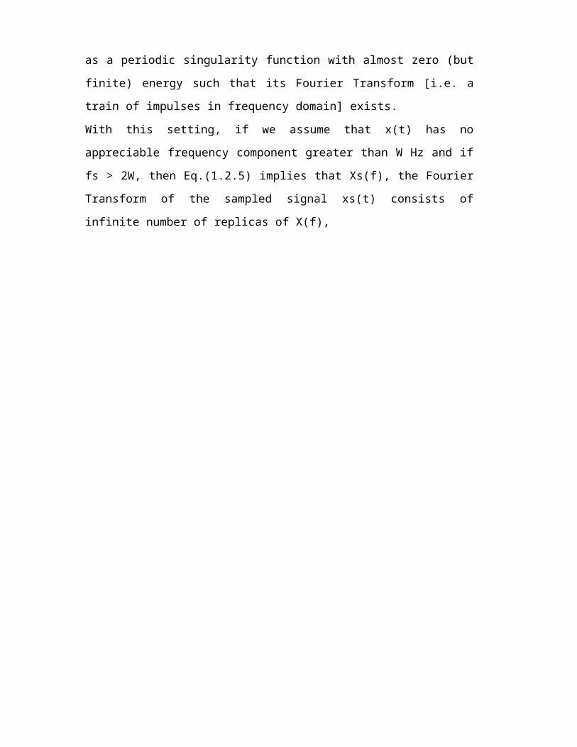
With this setting, if we assume that x(t) has no appreciable frequency component

greater than W Hz and if fs > 2W, then Eq.(1.2.5) implies that Xs(f), the Fourier

Transform of the sampled signal xs(t) consists of infinite number of replicas of X(f),

Fig. 1.3 Spectra of (a) an analog signal x(t) and (b) its sampled version

Fig. 1.3 indicates that the bandwidth of this instantaneously sampled wavexs(t) is infinite while the spectrum of x(t) appears in a periodic manner, centered at discrete frequency values n.fs.

Now, Part – I of the sampling theorem is about the condition fs > 2.W i.e. (fs – W) >W and (– fs + W) < – W. As seen from Fig. 1.3, when this condition is satisfied, the spectra of xs(t), centered at f = 0 and f = ± fs do not overlap and hence, the spectrum

centered at discrete frequencies n.fs, -∞ < n < ∞ and scaled by a constant fs= 1/Ts

(Fig. 1.3).

of x(t) is present in xs(t) without any distortion. This implies that xs(t), the

appropriately sampled version of x(t), contains all information about x(t) and thus

represents x(t).

The second part of Nyquist’s theorem suggests a method of recovering x(t) from its

sampled version xs(t) by using an ideal lowpass filter. As indicated by dotted lines in

Fig. 1.3, an ideal lowpass filter (with brick-wall type response) with a bandwidth W

≤ B < (fs – W), when fed with xs(t), will allow the portion of Xs(f), centered at f = 0

and will reject all its replicas at f = n fs, for n ≠ 0. This implies that the shape of the

continuous-time signal xs(t), will be retained at the output of the ideal filter.

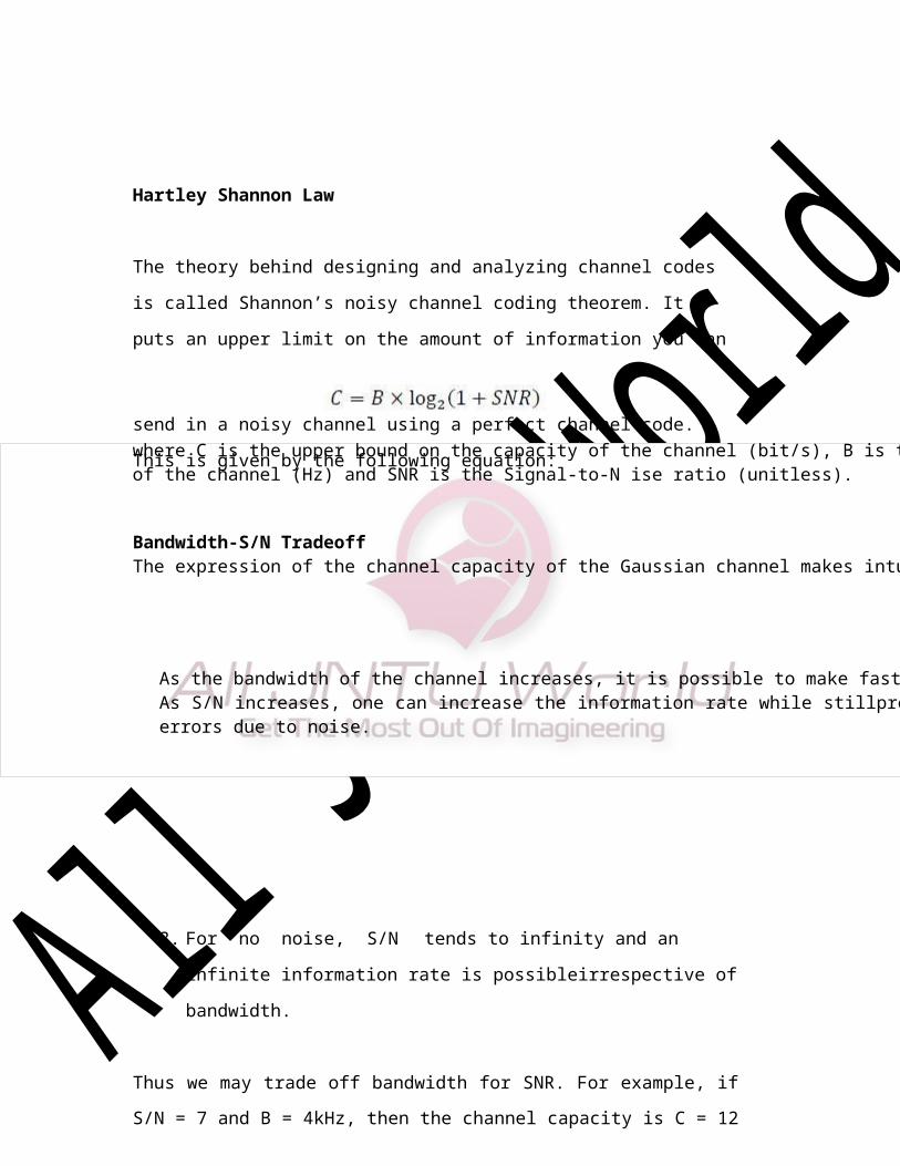
where C is the upper bound on the capacity of the channel (bit/s), B is the bandwidthof the channel (Hz) and SNR is the Signal-to-N ise ratio (unitless).

Bandwidth-S/N TradeoffThe expression of the channel capacity of the Gaussian channel makes intuitive sense:

As the bandwidth of the channel increases, it is possible to make faster changes in the information signal, thereby increasing the information rate.As S/N increases, one can increase the information rate while stillpreventingerrors due to noise.

Hartley Shannon Law

The theory behind designing and analyzing channel codes is called Shannon’s noisy

channel coding theorem. It puts an upper limit on the amount of information you can

send in a noisy channel using a perfect channel code. This is given by the following

equation:

3. For no noise, S/N tends to infinity and an infinite information rate is

possibleirrespective of bandwidth.

Thus we may trade off bandwidth for SNR. For example, if S/N = 7 and B = 4kHz,

then the channel capacity is C = 12 ×103 bits/s. If the SNR increases to S/N = 15 and

B is decreased to 3kHz, the channel capacity remains the same. However, as B tends

to 1, the channel capacity does not become infinite since, with an increase in

bandwidth, the noise power also increases. If the noise power spectral density is ɳ/2,

then the total noise power is N = ɳB, so the Shannon-Hartley law becomes

IntroductionIn the simplest model of a telephone speech communication there is a direct, dedicated, physical connection between the two participants in the conversation, and this link is held for the duration of the conversation. The analogue electrical signal produced by the telephone at either end is sent on to connection without modification.In Pulse Amplitude Modulation (PAM), the unmodified electrical signal is not sent on to the connection. Instead, short samples of the signal are taken at regular intervals, and these samples are sent on to the connection. The amplitude of each sample is identical to the signal voltage at the time when the sample was taken. Typically, 8,000 samples are taken per second, so that the interval between samples is 125s, and the duration of each sample is approximately 4s.

Pulse Code Modulation

Because each sample is very short (~4s) there is a lot of time between samples (~121s). Samples from other conversations are put into this “spare time”. Usually the samples from 32 separate conversations are put on to a single line. This process is called Time Division Multiplexing (TDM).

Each sample is very short, and will be distorted as it travels across a communications network. In order to reconstruct the original analogue signal the only information the receiver needs to have about a sample is its amplitude, but if this is distorted then all information about the sample has been lost. To overcome this problem, the pulse is not transmitted directly, instead its amplitude is measured and converted into an 8 binary number - a sequence of 1s and 0s. At the receiver end, the receiver merely needs to detect if a 1 or a 0 has been received so that it can still recover the amplitude of a PAM pulse even if the 1s and 0s used to describe it have been distorted.

The process of converting the amplitude of each pulse into a stream of 1s and 0s is called Pulse Code Modulation (PCM)

Note that the process of PAM and PCM (but without the use of TDM) is essentially used to store music and speech on CDs, but with a higher sample rate, more bits per sample and complex error correction mechanisms.

Some terms are:

Sampling The process of measuring the amplitude of a continuous-time signal at discrete instants. It converts a continuous-time signal to a discrete- time signal.

Quantizing Representing the sampled values of the amplitude by a finite set of levels. It converts a continuous-amplitude sample to a discrete- amplitude sample.

Encoding Designating each quantized level by a (binary) code.

Sampling and quantizing operations transform an analogue signal to a digital signal.

Use of quantizing and encoding distinguishes PCM from analogue pulse modulation methods.

The quantizing and encoding operations are usually performed in the same circuit at the transmitter, which is called an Analogue to Digital Converter (ADC). At the receiver end the decoding operation converts the (8 bit) binary representation of the pulse back into an analogue voltage in a Digital to Analogue Converter (DAC)

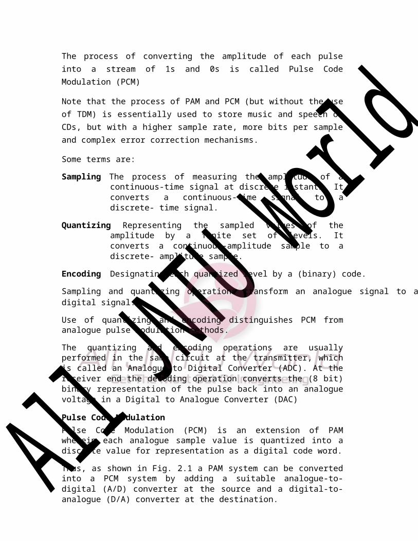
Pulse Code ModulationPulse Code Modulation (PCM) is an extension of PAM wherein each analogue sample value is quantized into a discrete value for representation as a digital code word.

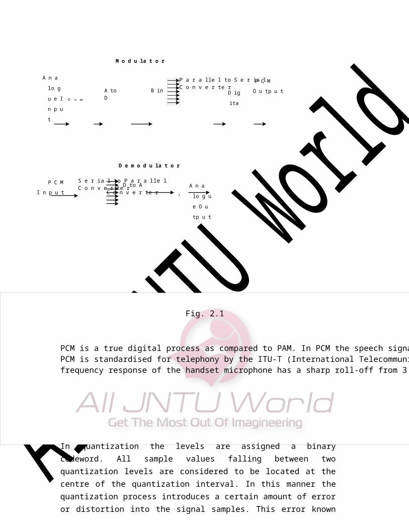
Thus, as shown in Fig. 2.1 a PAM system can be converted into a PCM system by adding a suitable analogue-to-digital (A/D) converter at the source and a digital-to- analogue (D/A) converter at the destination.

S a m p A to D

C o n v e

D ig

ita l P

u ls e

B in a

r y C

P a r a lle l to S e r ia lC o n v e r te r

D to AC o n v e r te r

S e r ia l to P a r a lle lC o n v e r te r

Fig. 2.1

PCM is a true digital process as compared to PAM. In PCM the speech signal is converted from analogue to digital form.PCM is standardised for telephony by the ITU-T (International Telecommunications Union - Telecoms, a branch of the UN), in a series of recommendations called the G series. For example the ITU-T recommendations for out-of-band signal rejection in PCM voice coders require that 14 dB of attenuation is provided at 4 kHz. Also, the ITU-T transmission quality specification for telephony terminals require that thefrequency response of the handset microphone has a sharp roll-off from 3.4 kHz.

M o d u la t o r

A n a lo g

u e I n p

u t

P C M

O u tp u t

D e m o d u la t o r

P C M

I n p u tA n a lo g

u e O u tp

u t

In quantization the levels are assigned a binary codeword. All sample values falling between two quantization levels are considered to be located at the centre of the quantization interval. In this manner the quantization process introduces a certain amount of error or distortion into the signal samples. This error known as quantization noise, is minimised by establishing a large number of small quantization intervals. Of course, as the number ofquantization intervals increase, so must the number or bits increase to uniquely identify the quantization intervals. For example, if an analogue voltage level is to be converted to a digital system with 8 discrete levels or quantization steps three bits are required. In the ITU-T version there are 256 quantization steps, 128 positive and 128 negative, requiring 8 bits. A positive level is represented by having bit 8 (MSB) at 0, and for a negative level the MSB is 1.

L P

Quantization

The process of quantizing a signal is the first part of converting an sequence of analog samples to a PCM code. In quantization, an analog sample with an amplitude that may take value in a specific range is converted to a digital sample with an amplitude that takes one of a specific pre–defined set of quantization values. This is performed by dividing the range of possible values of the analog samples into L different levels, and assigning the center value of each level to any sample that falls in that quantization interval. The problem with this process is that it approximates the value of an analog sample with the nearest of the quantization values. So, for almost all samples, the quantized samples will differ from the original samples by a small amount. This amount is called the quantization error. To get some idea on the effect of this quantization error, quantizing audio signals results in a hissing noise similar to what you would hear when play a random signal.

Assume that a signal with power Psis to be quantized using a quantizer with L = 2n levels ranging in voltage from –mp tomp as shown in the fig. 2.2

A quantization interval Corresponding quantization

value mp

v

L = 2n

L levels n bits 0

s 2Ts 3Ts

t4Ts 5

–mp

Q u an tizer In p u t S am p les xQ u an tizer O u tp u t S am p les x q

Fig. 2.2

We can define the variable v to be the height of the each of the L levels of the quantizer as shown above. This gives a value of v equal to

v 2 m p .L

Therefore, for a set of quantizers with the same mp, the larger the number of levels of a quantizer, the smaller the size of each quantization interval, and for a set of quantizers with the same number of quantization intervals, the larger mp is the larger the quantization interval length to accommodate all the quantization range.

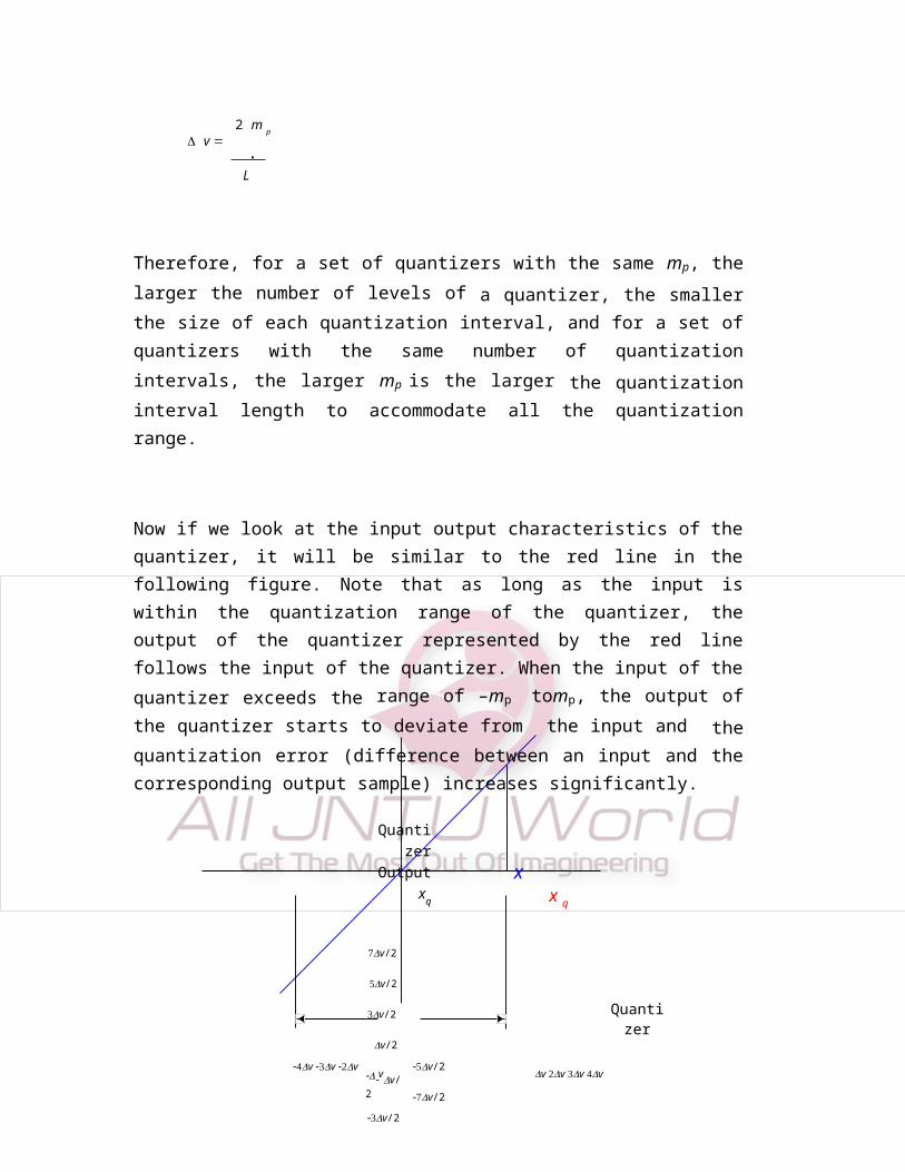
Now if we look at the input output characteristics of the quantizer, it will be similar to the red line in the following figure. Note that as long as the input is within the quantization range of the quantizer, the output of the quantizer represented by the red line follows the input of the quantizer. When the input of the quantizer exceeds the range of –mp tomp, the output of the quantizer starts to deviate from the input and the quantization error (difference between an input and the corresponding output sample) increases significantly.

Quantizer Output xq

v/2

v/2

v/2

v/2

xx q

Quantizerv v v

vv/2

v/2

v/2

v/2

v v v v Input x

mp

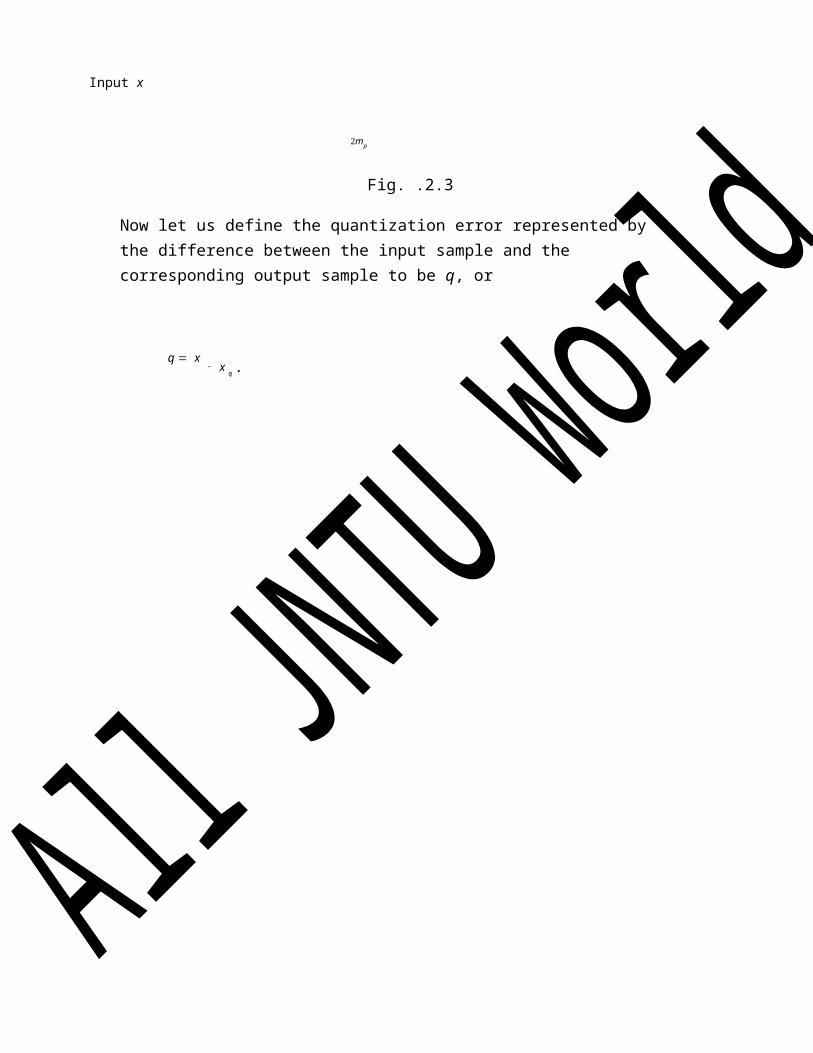
Fig. .2.3

Now let us define the quantization error represented by the difference between the input sample and the corresponding output sample to be q, or

q x x q .

Plotting this quantization error versus the input signal of a quantizer is seen next. Notice that the plot of the quantization error is obtained by taking the difference between the blow and red lines in the above Fig. 2.3

Quantization Error q

v/2 Quantizer

v v vv/2

v v v v vInput x

Fig. 2.4

It is seen from the Fig 2.4 that the quantization error of any sample is restricted between –v/2 andv/2 except when the input signal exceeds the range of quantization of –mp to mp.

Uniform Quantization

-m p +m p

I n p u t

We assume that the amplitude of the signal m(t) is confined to the range (-mp, +mp ). This range (2mp) is divided into L levels, each of step size , given by

= 2 mp / L

A sample amplitude value is approximated by the midpoint of the interval in which it lies. The input/output characteristics of a uniform quantizer is shown in Fig. 2.5

Fig. 2.5

O u

t

mp

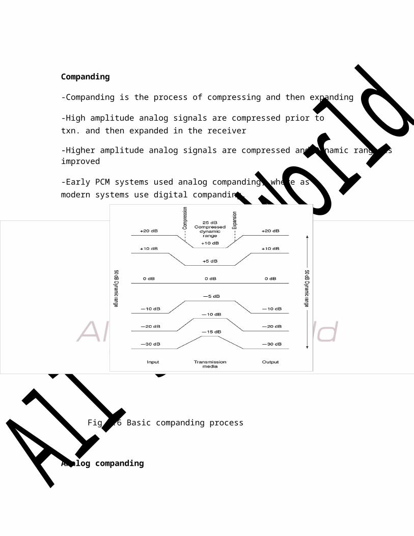
Companding

-Companding is the process of compressing and then expanding

-High amplitude analog signals are compressed prior to txn. and then expanded in the receiver

-Higher amplitude analog signals are compressed and Dynamic range is improved

-Early PCM systems used analog companding, where as modern systems use digital companding.

Fig 2.6 Basic companding process

Analog companding

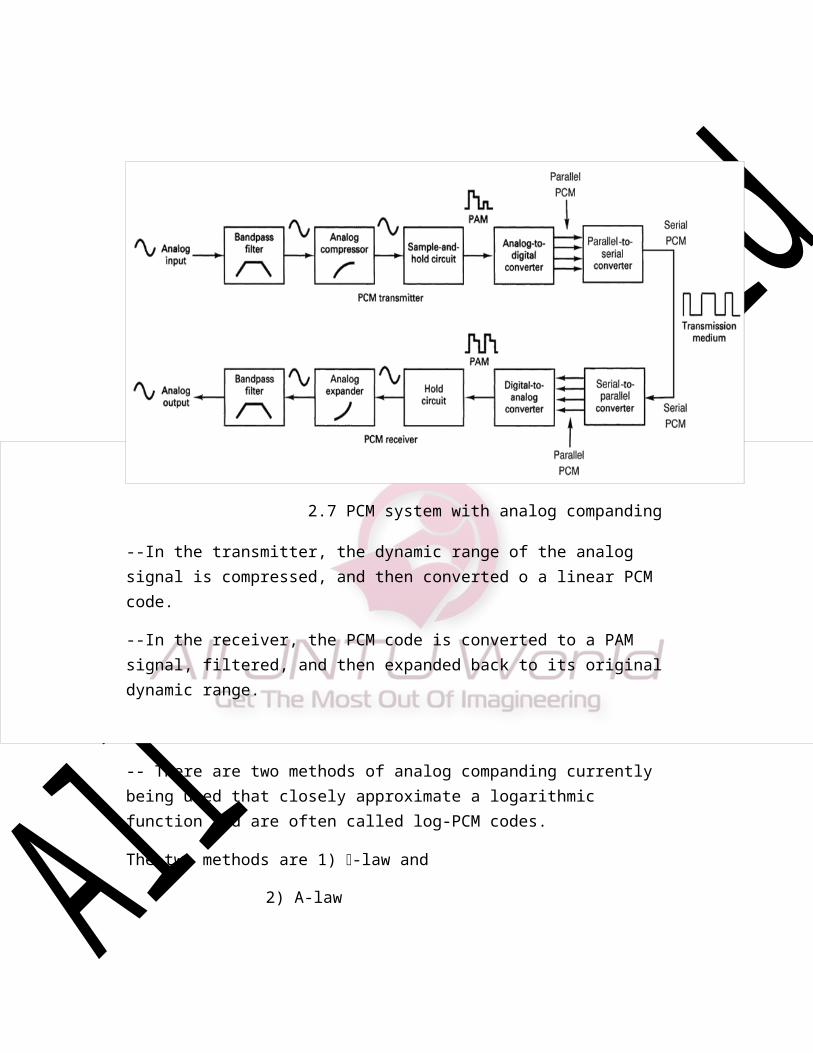
2.7 PCM system with analog companding

--In the transmitter, the dynamic range of the analog signal is compressed, and then converted o a linear PCM code.

--In the receiver, the PCM code is converted to a PAM signal, filtered, and then expanded back to its original dynamic range.

-- There are two methods of analog companding currently being used that closely approximate a logarithmic function and are often called log-PCM codes.

The two methods are 1) -law and

2) A-law

-law companding

where Vmax = maximum uncompressed analog input amplitude(volts) Vin = amplitude of the input signal at a particular instant of time (volts) = parameter used tio define the amount of compression (unitless)Vout = compressed output amplitude (volts)

A-law companding

V m a x ln 1 V in

V

V out m a x

ln 1

Fig. 2.8m-law companding

--A-law is superior to -law in terms of small-signal quality

--The compression characteristic is given by

where y = Vout

A | x | 1 log A

, 10 | x | A

Vmaxy 1 log(

A | x |) 1

, | x | 1x = Vin /

1 log A A

%error=12-bit encoded voltage - 12-bit decoded voltage X 100

12-bit decoded voltage

1.3 PCM Encoding Process (HDB3)The output from the analogue to digital converter (ADC) has n parallel bits. In the case of telephony n = 8. The most significant bit is the signed bit. If the measured sample is positive then the signed bit is 0. If the measured sample is negative then

Digital Companding:

--With digital companding, the analog signal is first sampled and converted to a linear PCM code, and then the linear code is digitally compressed.

-- In the receiver, the compressed PCM code is expanded and then decoded back to analog.

-- The most recent digitally compressed PCM systems use a 12- bit linear PCM code and an 8-bit compressed PCM code.

Digital compression error

--To calculate the percentage error introduced by digital compression

the signed bit is 1. The remaining 7 bits are used to code the sample value. The ITU- T define a look up table which allocates a particular binary code to each quantified A-law value.

The line coding which is used assigns opposite polarities to successive “1”s. This eliminates any DC voltage on the line, and reduces the inter symbol interference if adjacent bits are “1”. If there is silence on the PCM channel then the measured samples will be 0 Vrms and the output of the DAC will be 1000 0000. A stream of all zeros is not desirable on an active channel because

all zeros could also be a fault condition and

it is difficult to recover the clock signal from the incoming signal.The coding system HDB3 is used and was developed to eliminate all zeros, and to assign opposite polarities to successive “1”s.

This is a bipolar signalling technique (i.e. relies on the transmission of both positive and negative pulses).

In AMI positive and negative pulses (of equal amplitude) are used for alternative symbols 1. No pulse is used for symbol 0. In either case the pulse returns to 0 before the end of the bit interval. This eliminates any DC on the line.

HDB3 encoding rules follow those for AMI, except that a sequence of four consecutive 0's are encoded using a special "violation" bit. The 4 th 0 bit is given the same polarity as the last 1-bit which was sent using the AMI encoding rule. This prevents long runs of 0's in the data stream which may otherwise prevent a receiver from tracking the centre of each bit. By introducing violations, extra "edges" are introduced, enabling a Digital PLL to reliably reconstruct the clock signal at the receiver. The HDB3 is transparent to the sequence of bits being transmitted (i.e. whatever data is sent, the Digital PLL can reconstruct the data and extract the bits at the receiver).

To prevent a DC being introduced by excessive runs of zeros any run of more than four zeros encodes as B00V. The value of B is assigned + or - alternately throughout the bit stream.

Example 1 1 1 1 1 1 1 1 = + - + - + - + -

B BBBBBBB

1 0 1 0 1 0 1 0 = + 0 - 0 + 0 - 0B 0 B 0 B 0 B 0

1 0 0 0 0 0 0 1 + 0 0 0 + 0 0 -= B 0 0 0 V 0 0 B

1 0 0 0 0 1 1 0 = + 0 0 0 + - + 0

= B 0 0 0 V B B 0

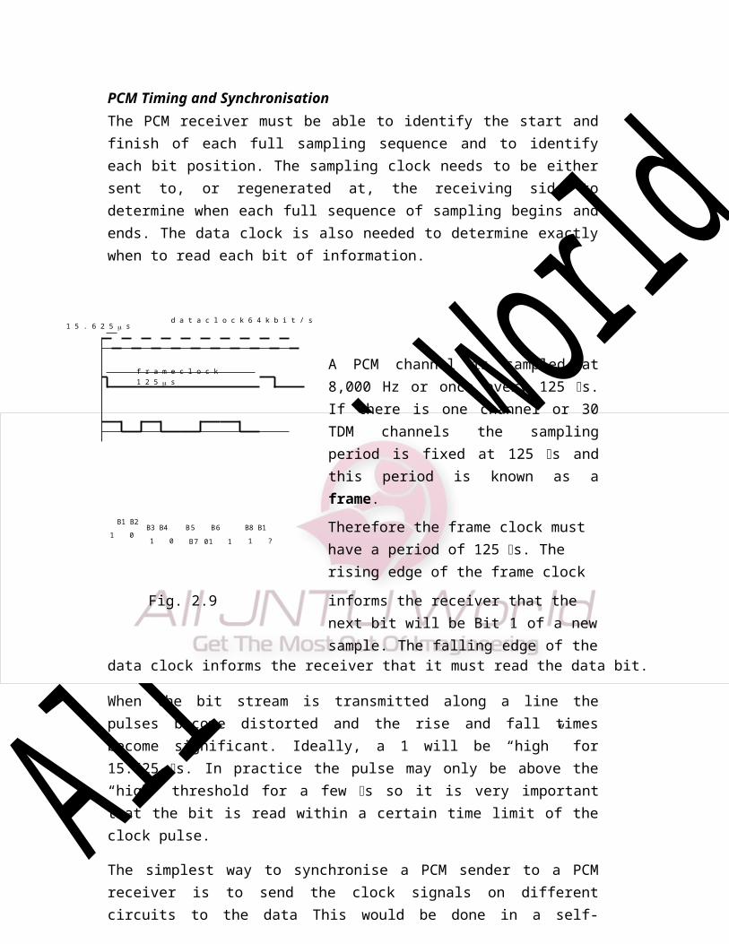
PCM Timing and SynchronisationThe PCM receiver must be able to identify the start and finish of each full sampling sequence and to identify each bit position. The sampling clock needs to be either sent to, or regenerated at, the receiving side to determine when each full sequence of sampling begins and ends. The data clock is also needed to determine exactly when to read each bit of information.

1 5 . 6 2 5 sd a t a c l o c k 6 4 k b i t / s

f r a m e c l o c k 1 2 5 s A PCM channel is sampled at 8,000 Hz or once every 125 s. If there is one channel or 30 TDM channels the sampling period is fixed at 125 s and this period is known as a frame.

B1 B2

1 0B3 B4

1 0

B5 B6 B7

0 1 1

B8 B1

1 ?Therefore the frame clock must have a period of 125 s. The rising edge of the frame clock

Fig. 2.9 informs the receiver that the next bit will be Bit 1 of a new sample. The falling edge of the

data clock informs the receiver that it must read the data bit.

When the bit stream is transmitted along a line the pulses become distorted and the rise and fall times become significant. Ideally, a 1 will be “high” for 15.625 s. In practice the pulse may only be above the “high” threshold for a few s so it is very important that the bit is read within a certain time limit of the clock pulse.

The simplest way to synchronise a PCM sender to a PCM receiver is to send the clock signals on different circuits to the data This would be done in a self-contained system such as private branch exchange (PBX). Telephony is full duplex so that there is a coder and a decoder at each port, but each would use the same clock.

To minimise the number of circuits it is possible to use a line-coding scheme which allows the receiver to extract the clocks from the PCM signal. In this case the receiver will have free running clocks that lock (using a PLL) to the phase and frequency of the transitions in the data stream. The line-coding scheme ensures that there is a transition for every data bit.

Differential pulse coding schemesPCM transmits the absolute value of the signal for each frame. Instead we can transmit information about the difference between each sample. The two main differential coding schemes are: Delta Modulation Differential PCM and Adaptive Differential PCM (ADPCM)

good as PCM.

To reconstruct the original from the quantization, if a 1 is received the signal is increased by a step of size q, if a 0 is received the output is reduced by the same size step. Slope overload occurs when the encoded waveform is more than a step size away from the input signal. This condition happens when the rate of change of the input exceeds the maximum change that can be generated by the output. Overload willoccurif:dx(t)/dt q /T = q * fs

where: x(t) = input signal, q = step size, T = period between samples, fs = sampling frequency

Delta ModulationDelta modulation converts an analogue signal, normally voice, into a digital signal.

The analogue signal is sampled as in theg r a n u la r n o i

s e 1 1

1

1 0 0 1

1 1 0

0 01

0 0 0

0

PCM process. Then the sample is compared with the previous sample. The result of the comparison is quantified using a one bit coder. If the sample is greater than the previous sample a 1 is generated. Otherwise a 0 is generated.The advantage of delta modulation over

PCM is its simplicity and lower cost. But the noise performance is not as Fig. 2.10

Assume that the input signal has maximum amplitude A and maximum frequency F. The most rapidly changing input is provided by x(t) = A * sin (2 * * F * t). For this dx(t)/dt = 2 * * F * A * sin (2 * * F * t). This slope has a maximum value of 2 * * F * AOverload occurs if 2 * * F * A > q * fs

To prevent overload we require q * fs> 2 * * F * AExample A = 2 V, F = 3.4 kHz, and the signal is sampled 1,000,000 times per second, requires q > 2 * 3.14 * 3,400 * 2 /1,000,000 V > 42.7 mV

Granular noise occurs if the slope changes more slowly than the step size. The reconstructed signal oscillates by 1 step size in every sample. It can be reduced by decreasing the step size. This requires that the sample rate be increased. Delta Modulation requires a sampling rate much higher than twice the bandwidth. It requires oversampling in order to obtain an accurate prediction of the next input, since each encoded sample contains a relatively small amount of information. Delta Modulation requires higher sampling rates than PCM.

Differential PCM (DPCM) and ADPCM

A n a l o g u e I n p u t

D i f f e r e n t ia t o r

+

E n c o d e d D i f f e r e n c e S a m p le s

-

Fig. 2.11

DPCM is also designed to take advantage of the redundancies in a typical speech waveform. In DPCM the differences between samples are quantized with fewer bits that would be used for quantizing an individual amplitude sample. The sampling rate is often the same as for a comparable PCM system,

unlike Delta Modulation.

Adaptive Differential Pulse Code Modulation ADPCM is standardised by ITU-T recommendations G.721 and G.726. The method uses 32,000 bits/s per voice channel, as compared to standard PCM’s 64,000 bits/s. Four bits are used to describe each sample, which represents the difference between two adjacent samples. Sampling is 8,000 times a second. It makes it possible to reduce the bit flow by half while maintaining an acceptable quality. While the use of ADPCM (rather than PCM) is imperceptible to humans, it can significantly reduce the throughput of high speed modems and fax transmissions.

The principle of ADPCM is to use our knowledge of the signal in the past time to predict the signal one sample period later, in the future. The predicted signal is then compared with the actual signal. The difference between these is the signal which is sent to line - it is the error in the prediction. However this is not done by making

A c c u m u l a to r D

B a n d L i m it i n g F i l

Q u a n t is e r E n o d e r

ADPCM is sometimes used by telecom operators to fit two speech channels onto a single 64 kbit/s link. This was very common for transatlantic phone calls via satelliteup until a few years ago. Now, nearly all calls use fibre optic channels at 64 kbit/s.

6.9 Delta Modulation

comparisons on the incoming audio signal - the comparisons are done after PCM coding.

To implement ADPCM the original (audio) signal is sampled as for PCM to produce a code word. This code word is manipulated to produce the predicted code word for the next sample. The new predicted code word is compared with the code word of the second sample. The result of this comparison is sent to line. Therefore we need to perform PCM before ADPCM.

The ADPCM word represents the prediction error of the signal, and has no significance itself. Instead the decoder must be able to predict the voltage of the recovered signal from the previous samples received, and then determine the actual value of the recovered signal from this prediction and the error signal, and then to reconstruct the original waveform.

Delta modulation, like DPCM is a predictive waveform coding technique and can be considered as a special case of DPCM. It uses the simplest possible quantizer, namely a two level (one bit) quantizer. The price paid for achieving the simplicity of the quantizer is the increased sampling rate (much higher than the Nyquist rate) and the possibility of slope-overload distortion in the waveform reconstruction, as explained in greater detail later on in this section.

In DM, the analog signal is highly over-sampled in order to increase the adjacent sample correlation. The implication of this is that there is very little change in two

adjacent samples, thereby enabling us to use a simple one bit quantizer, which like in DPCM, acts on the difference (prediction error) signals.

In its original form, the DM coder approximates an input time function by a series of linear segments of constant slope. Such a coder is therefore referred to as a Linear (or non-adaptive) Delta Modulator (LDM). Subsequent developments have resulted in delta modulators where the slope of the approximating function is a variable. Such coders are generally classified under Adaptive Delta Modulation (ADM) schemes. We use DM to indicate either of the linear or adaptive variety.

Fig. 2.12: Waveforms illustrative of LDM operation

Deltamodulation principleofoperation

Deltamodulationwasintroducedinthe1940sasasimplifiedformofpulsecodemodulatio n(PCM),whichrequiredadifficult-to-implementanalog-to-digital(A/D)converter.

Theoutputofadeltamodulatorisabitstreamofsamples,atarelatively highrate(eg,100kbit/sor

moreforaspeechbandwidthof4 kHz)thevalueofeachbitbeing determinedaccordingas towhethertheinputmessagesampleamplitudehasincreasedordecreasedrelativetothepr evioussample.Itisan exampleofdifferentialpulsecodemodulation(DPCM).

Blockdiagram

Theoperationofadeltamodulatoristoperiodicallysampletheinputmessage,tomakeac omparisonofthecurrentsamplewiththatprecedingit,andtooutputasinglebit which indicatesthesignofthe differencebetweenthe twosamples.Thisinprinciple would requirea sample-and-hold type circuit.

DeJager(1952)hitonanideafordispensingwiththeneedforasampleandholdcircuit.Her easonedthatifthesystemwasproducingthedesiredoutputthenthisoutputcouldbesentb acktotheinputandthetwoanalogsignalscomparedinacomparator.Theoutput isa delayedversionoftheinput,andsothecomparison isineffectthatofthecurrentbitwiththepreviousbit,asrequiredbythedeltamodulationpri nciple.

Figure2.13illustratesthebasicsysteminblockdiagramform,andthiswillbethemodulat oryouwill bemodelling.

Thesystemisintheformofafeedbackloop.Thismeansthatitsoperationisnotn ecessaril

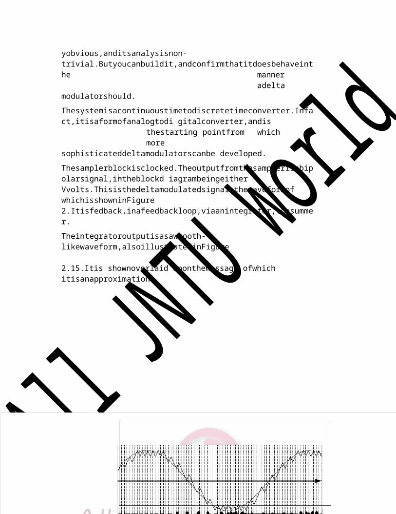
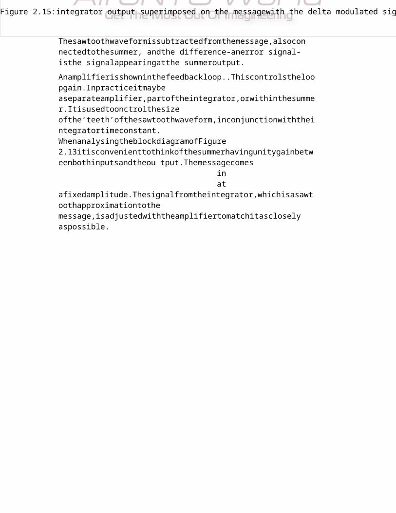
Figure 2.15:integrator output superimposed on the messagewith the delta modulated signal below

yobvious,anditsanalysisnon- trivial.Butyoucanbuildit,andconfirmthatitdoesbehaveinthe manner adelta modulatorshould.

Thesystemisacontinuoustimetodiscretetimeconverter.Infact,itisaformofanalogtodi gitalconverter,andis thestarting pointfrom which more sophisticateddeltamodulatorscanbe developed.

Thesamplerblockisclocked.Theoutputfromthesamplerisabipolarsignal,intheblockd iagrambeingeither Vvolts.Thisisthedeltamodulatedsignal,thewaveformof whichisshowninFigure 2.Itisfedback,inafeedbackloop,viaanintegrator,toasummer.

Theintegratoroutputisasawtooth-likewaveform,alsoillustratedinFigure 2.15.Itis shownoverlaid uponthemessage,ofwhich itisanapproximation.

Thesawtoothwaveformissubtractedfromthemessage,alsoconnectedtothesummer, andthe difference-anerror signal-isthe signalappearingatthe summeroutput.

Anamplifierisshowninthefeedbackloop..Thiscontrolstheloopgain.Inpracticeitmaybe aseparateamplifier,partoftheintegrator,orwithinthesummer.Itisusedtoonctrolthesize ofthe‘teeth’ofthesawtoothwaveform,inconjunctionwiththeintegratortimeconstant.WhenanalysingtheblockdiagramofFigure 2.13itisconvenienttothinkofthesummerhavingunitygainbetweenbothinputsandtheou tput.Themessagecomes in at afixedamplitude.Thesignalfromtheintegrator,whichisasawtoothapproximationtothe message,isadjustedwiththeamplifiertomatchitasclosely aspossible.

stepsizecalculation

InthedeltamodulatorofFigure2.13theoutputoftheintegratorisasawtooth- likeapproximationtotheinputmessage.Theteethofthesaw mustbeabletorise(orfall)fastenoughtofollowthemessage.Thustheintegratortimecons tantisanimportantparameter.

Foragivensampling(clock)ratethestepslope(volt/s)determinesthesize(volts)oftheste p withinthesamplinginterval.

Supposetheamplitudeof therectangularwavefromthesampleris±V volt.Forachangeofinputsampleto theintegratorfrom(say)negativeto positive,thechangeofintegrator output will be,

afteraclockperiodT:

wherekisthegainoftheamplifier precedingthe integrator(asinFigure2.13).

AnswerTutorialQuestions1and 2beforeattemptingtheexperiment.Youcanlatercheckyouranswerbymeasurement.

slopeoverloadandgranularity

ThebinarywaveformillustratedinFigure2.15isthesignaltransmitted.Thisisthedeltamo dulatedsignal.

Theintegralofthebinarywaveformisthesawtoothapproximationto themessage.

IntheexperimententitledDeltademodulation(inthisVolume)youwillseethatthissawto othwave istheprimaryoutputfromthedemodulatoratthereceiver.

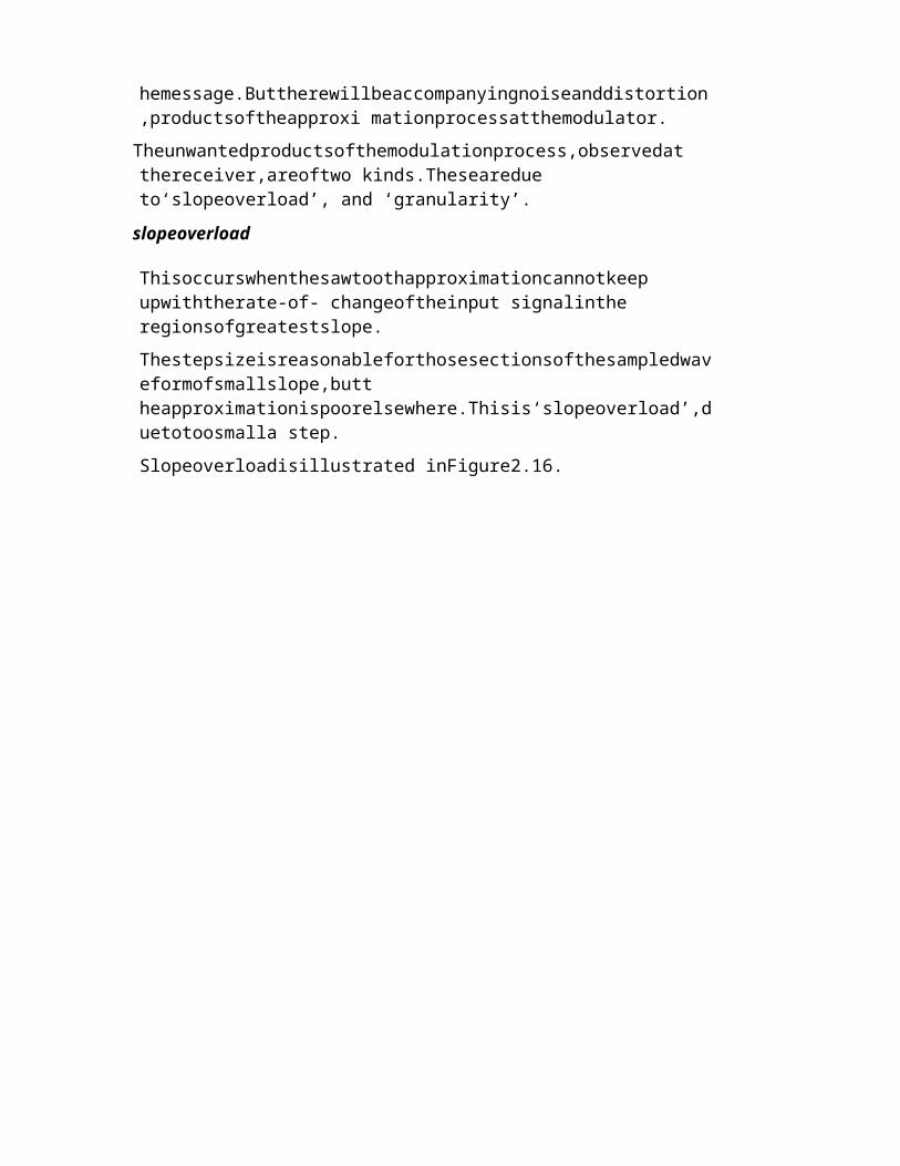
Lowpassfilteringofthesawtooth(fromthedemodulator)givesabetterapproximationtot hemessage.Buttherewillbeaccompanyingnoiseanddistortion,productsoftheapproxi mationprocessatthemodulator.

Theunwantedproductsofthemodulationprocess,observedatthereceiver,areoftwo kinds.Thesearedue to‘slopeoverload’, and ‘granularity’.

slopeoverload

Thisoccurswhenthesawtoothapproximationcannotkeepupwiththerate-of- changeoftheinput signalinthe regionsofgreatestslope.

Thestepsizeisreasonableforthosesectionsofthesampledwaveformofsmallslope,butt heapproximationispoorelsewhere.Thisis‘slopeoverload’,duetotoosmalla step.

Slopeoverloadisillustrated inFigure2.16.

slo p e o v e rlo a d

Figure2.16:slopeoverload

Toreducethepossibilityofslopeoverloadthestepsizecanbeincreased(forthesamesamp ling rate).This isillustratedin Figure 2.17.Thesawtoothisbetterabletomatchthemessageinthe regionsofsteep slope.

Figure2.17:increasedstepsize to reduce slope overload

An alternative method of slope overload reduction is to increase the samplingrate.This is illustrateFigure2.18,wheretheratehasbeenincreasedbyafactorof2.4times, but thestep isthe same size asinFigure2.15.

1.4 Granularnoise

ReferbacktoFigure 2.16.Thesawtoothfollowsthemessagebeingsampledquitewellintheregionsofsmallslo pe.Toreducetheslopeoverloadthestepsizeisincreased,andnow(Figure 2.17)thematchovertheregionsofsmallslopehasbeendegraded.

Thedegradationshowsup,atthedemodulator,asincreasedquantizingnoise,or‘granulari ty’.

1.5 noiseanddistortionminimization

Figure2.18:increasedsampling rate to reduce slope overload

Thereisaconflictbetweentherequirementsforminimizationofslopeoverloadandthegra nularnoise.Theonerequiresanincreasedstepsize,theotherareducedstepsize.You shouldrefertoyourtextbook formorediscussion ofwaysandmeansofreachingacompromise.Youwillmeetanexampleintheexperimente ntitledAdaptivedeltamodulation(inthisVolume).Anoptimumstepcanbedeterminedby minimizingthequantizingerroratthesummer output, or thedistortionatthe demodulatoroutput.

Adaptive Delata Modulation

tim e

The Operation Theory of ADM Modulation

From previous chapter, we know that the disadvantage of delta modulation is when the input audio signal frequency exceeded the limitation of delta modulator, i.e.

Then this situation will produce the occurrence of slope overload and cause signal distortion. However, the adaptive delta modulation (ADM) is the modification of delta modulation to improve the disadvantage of the occurrence of slope overload.

Figure 2.20 is the block diagram of ADM modulator. In figure 2.20, we can see that the delta modulator is comprised by comparator, sampler and integrator, then the slope controller and the level detect algorithm comprise a quantization level adjuster, which can control the gain of the integrator in the delta modulator. ADM modulator is the modification of delta modulator, therefore, due to the delta modulator has the problem of slope overload at low and high frequencies. The reason is the magnitude of the Δ(t) of delta modulator is fixed, i.e. the increment of Δ or -Δ is unable to follow the variation of the slope of the input signal. When the variation of the slope of the input signal is large, the magnitude of Δ(t) still can increase by following the variation, then this situation will not occur the problem of slope overload. On the other hand, there is another technique, which is known as continuous variable slope delta (CVSD) modulation. This technique is commonly used in Bluetooth application. CVSD modulator is also the modification of delta modulator, use to improve the occurrence of slope overload. The different between the CVSD and ADM modulators are the quantization level adjuster A. ADM modulator is discrete values and the quantization level adjuster of CVSD modulator is continuous. Simply, the quantization value of ADM modulator is the variation of digital, such as the quantization values of +1, +2, +3, -2, -3 and so on. As for CVSD modulator, the quantization value is the variation of analog, such as the quantization values of +1,+1.1, +1.2, -1.5, -0.3, -0.9 and so on.

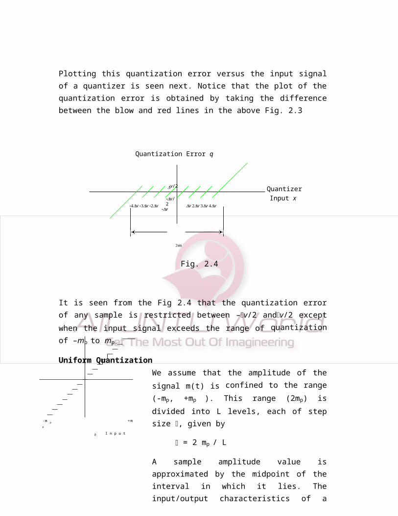
Fig. 2.20 The Operation Theory of ADM Modulation

UNIT - II

Digital modulation techniquesModulation is defined as the process by which some characteristics of a carrier is

varied in accordance with a modulating wave. In digital communications, the

modulating wave consists of binary data or an M-ary encoded version of it and the

carrier is sinusoidal wave.

Different Shift keying methods that are used in digital modulation techniques are

Amplitude shift keying [ASK]

Frequency shift keying [FSK]

Phase shift keying [PSK]

In a binary ASK system symbol ‘1’ and ‘0’ are transmitted as

S (t) 1

2EbTb

Cos2f t for symbol 11

S 2 (t) 0 for symbol 0

2. FSK[Frequency Shift Keying]:

In a binary FSK system symbol ‘1’ and ‘0’ are transmitted as

1 1

Fig 3.1 Different modulations1. ASK[Amplitude Shift Keying]:

S (t) 2E b Cos2f t for symbol 1

T b

S 2(t) 2Eb Cos2f 2t for symbol 0Tb

3. PSK[Phase Shift Keying]:

In a binary PSK system the pair of signals S1(t) and S2(t) are used to represent binary symbol ‘1’ and ‘0’ respectively.

S1 (t) 2Eb Cos2fc t --------- for Symbol ‘1’Tb

S2 (t) 2Eb Cos(2fc t ) 2Eb Cos2fc t ------- for Symbol ‘0’Tb Tb

Hierarchy of digital modulation technique

Digital Modulation Technique

Coherent Non - Coherent

Binary M - ary Hybrid Binary M - ary(m) = 2 (m) = 2

* ASK M-ary ASK M-ary APK * ASK M-ary ASK* FSK M-ary FSK M-ary QAM * FSK M-ary FSK* PSK M-ary PSK * DPSK M-ary DPSK

(QPSK)

(t) 2Cos2f t1 c

Tb

x(t) x1 Choose 1 if x1>0

Choose 0 if x1<0

Correlator1 (t) Threshold λ = 0

Fig 3.3 Coherent binary PSK receiver

In a Coherent binary PSK system the pair of signals S1(t) and S2(t) are used

Decision DeviceT b

dt0

Coherent Binary PSK:

BinaryData Sequence

Fig. 3.2 Block diagram of BPSK transmitter

to represent binary symbol ‘1’ and ‘0’ respectively.

S1 (t) 2Eb Cos2fc t --------- for Symbol ‘1’Tb

S2 (t) 2Eb Cos(2fc t ) 2Eb Cos2fc t ------- for Symbol ‘0’Tb Tb

Where Eb= Average energy transmitted per bit Eb E E

b0 b1

2In the case of PSK, there is only one basic function of Unit energy which is given

by

Non Return toProductZero Level

Encoder ModulatorBinary PSK Signal

2 T

b

E

E

Eb

Tb

0

The message point corresponding to S1(t) is located at S11 Eb and S2(t) is located at S21 Eb .To generate a binary PSK signal we have to represent the input binary sequence inpolar form with symbol ‘1’ and ‘0’ represented by constant amplitude levels of

S21 S2 (t)1 (t) dt Eb

Eb & Eb respectively. This signal transmission encoding is performed by a NRZ

level encoder.The resulting binary wave [in polar form] and a sinusoidal carrier 1 (t)[whose frequency fc nc ] are applied to a product modulator. The desired BPSK waveTb

(t) Cos2f t 0 t T1 c b

Therefore the transmitted signals are given bySymbol

S (t) (t) 0 t T for 11 b 1 B

S (t) (t) 0 t T

2 b 1 B

for Symbol 0

A Coherent BPSK is characterized by having a signal space that is one dimensional (N=1) with two message points (M=2)

Tb

S11 S1 (t)1 (t) dt 0

is obtained at the modulator output.

To detect the original binary sequence of 1’s and 0’s we apply the noisy PSK

signal x(t) to a Correlator, which is also supplied with a locally generated coherent

reference signal 1 (t) as shown in fig (b). The correlator output x1 is compared with a

threshold of zero volt.

If x1 > 0, the receiver decides in favour of symbol 1.

If x1 < 0, the receiver decides in favour of symbol 0.

Therefore FSK is characterized by two dimensional signal space with two message points i.e. N=2 and m=2.

The two message points are defined by the signal vector

Generation and Detection:-

Coherent Binary FSK

In a binary FSK system symbol ‘1’ and ‘0’ are transmitted as

S (t)

2E b Cos2f t for symbol 1

1 Tb1

S 2(t) 2Eb Cos2f 2t for symbol 0Tb

The basic functions are given by

(t) 2 Cos2ft AndT

b1 1

(t) 2 Cos2ft for 0 t T And Zero Otherwise2 Tb

2 b

(a)

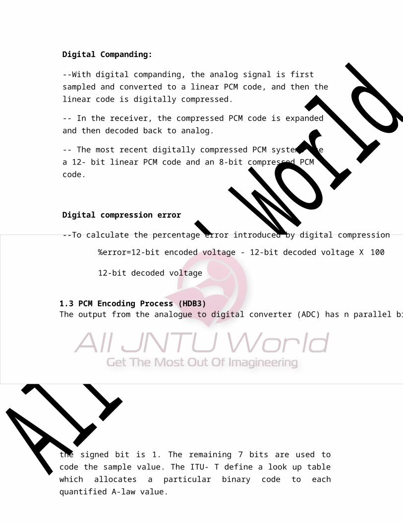
Fig. 3.4: (a) FSK transmitter ( b) FSK Receiver

A binary FSK Transmitter is as shown in fig. (a). The incoming binary data sequence is applied to on-off level encoder. The output of encoder is Eb volts for symbol 1 and 0 volts for symbol ‘0’. When we have symbol 1 the upper channel isswitched on with oscillator frequency f1, for symbol ‘0’, because of inverter the lowerchannel is switched on with oscillator frequency f2. These two frequencies are combined using an adder circuit and then transmitted. The transmitted signal is nothing but required BFSK signal.The detector consists of two correlators. The incoming noisy BFSK signal x(t) iscommon to both correlator. The Coherent reference signal 1 (t) and 2 (t) are supplied

(b)

to upper and lower correlators respectively.

The correlator outputs are then subtracted one from the other and resulting a

random vector ‘l’ (l=x1 - x2). The output ‘l’ is compared with threshold of zero volts.

If l > 0, the receiver decides in favour of symbol 1.

l < 0, the receiver decides in favour of symbol0

Product Modulator

ON-OFFLevel Encod

x(t) X If x > λ choose symbol 1

If x < λ choose symbol 01 (t)Threshold λ

Fig. 3.6 Coherent binary ASK demodulator In Coherent binary ASK system the basic function is given by

(t) 2 Cos2f t 0 t T1 e b

TbThe transmitted signals S1(t) and S2(t) are given by S1 (t) Eb 1 (t) for Symbol 1S2 (t) 0 for Symbol 0

Decision DeviceTb

dt0

BINARY ASK SYSTEM :-

BinaryData Sequence

Binary ASK Signal

Fig. 3.5 BASK transmitter

(t) 2 Cos2f t

1 e

Tb

The BASK system has one dimensional signal space with two messages (N=1, M=2)

MessagePoint 2

Eb

1 (t)

output Eb volts for symbol 1 and 0 volt for symbol 0. The resulting binary wave [in unipolarform] and sinusoidal carrier 1 (t) are applied to a product modulator. The desired BASK wave is obtained at the modulator output.

In demodulator, the received noisy BASK signal x(t) is apply to correlator with coherent reference signal 1 (t) as shown in fig. (b). The correlator output x is compared with threshold λ.If x > λ the receiver decides in favour of symbol 1.If x < λ the receiver decides in favour of symbol 0.

Incoherent detection:

Region E2 Region E1

0E

b Message2 Point 1

Fig. 3.7 Signal Space representation of BASK signal

In transmitter the binary data sequence is given to an on-off encoder. Which gives an

Fig. 3.8 : Envelope detector for OOK BASK

Fig. 3.9 : Incoherent detection of FSK

Fig. 3.9 shows the block diagram of incoherent type FSK demodulator. The detector consists of two band pass filters one tuned to each of the two frequencies used tocommunicate ‘0’s and ‘1’s., The output of filter is envelope detected and then baseband detectedusing an integrate and dump operation. The detector is simply evaluating which of two possible

Incoherent detection as used in analog communication does not require carrier for

reconstruction. The simplest form of incoherent detector is the envelope detector as shown in

Fig. 3.8. The output of envelope detector is the baseband signal. Once the baseband signal is

recovered, its samples are taken at regular intervals and compared with threshold.

If Z(t) is greater than threshold ( ) a decision will be made in favour of symbol ‘1’

If Z(t) the sampled value is less than threshold ( ) a decision will be made in favour of

symbol ‘0’.

Non- Coherenent FSK Demodulation:-

sinusoids is stronger at the receiver. If we take the difference of the outputs of the two envelope

detectors the result is bipolar baseband.

The resulting envelope detector outputs are sampled at t = kTb and their values are

compared with the threshold and a decision will be made infavour of symbol 1 or 0.

Differential Phase Shift Keying:- [DPSK]

(b) DPSK Receiver Fig. 3.10 DPSKA DPSK system may be viewed as the non coherent version of the PSK. It eliminates the need for coherent reference signal at the receiver by combining two basic operations at the transmitterDifferential encoding of the input binary wave andPhase shift keying

(a) DPSK Transmitter

Hence the name differential phase shift keying [DPSK]. To send symbol ‘0’ we

phase advance the current signal waveform by 1800 and to send symbol 1 we leave the

phase of the current signal waveform unchanged.

The differential encoding process at the transmitter input starts with an arbitrary

first but, securing as reference and thereafter the differentially encoded sequence{dk} is

generated by using the logical equation.

d k d k 1 bk

d k 1 bk

Where bk is the input binary digit at time kTb and dk-1 is the previous value of the

A DPSK demodulator is as shown in fig(b). The received signal is first passed through a BPF centered at carrier frequency fc to limit noise power. The filter output and its delay version are applied to correlator the resulting output of correlator is proportionalto the cosine of the difference between the carrier phase angles in the two correlatorinputs. The correlator output is finally compared with threshold of ‘0’ volts . If correlator output is +ve-- A decision is made in favour of symbol ‘1’ If correlator output is -ve--- A decision is made in favour of symbol ‘0’

differentially encoded digit. Table illustrate the logical operation involved in the generation of DPSK signal.

Input Binary Sequence {bK} 1 0 0 1 0 0 1 1Differentially Encoded 1 1 0 1 1 0 1 1 1sequence {dK}

Transmitted Phase 0 0 Π 0 0 Π 0 0 0Received Sequence 1 0 0 1 0 0 1 1

(Demodulated Sequence)

Fig. 3.11(b) QPSK ReceiverIn case of QPSK the carrier is given by

COHERENT QUADRIPHASE – SHIFT KEYING

Fig. 3.11(a) QPSK Transmitter

s (t) 2E Cos[2f t (2i 1) / 4] 0 t T i 1 to 4i T c

s (t)

2E Cos[(2i 1) / 4]cos( 2f t) 2E sin[(2i 1) / 4]sin( 2f t) 0 t T i 1 to 4

i T c T c

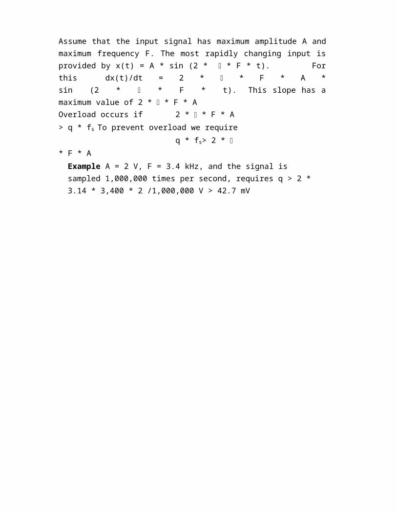
Fig. 3.11(c) QPSK Waveform

In QPSK system the information carried by the transmitted signal is contained in

the phase. The transmitted signals are given by

Where the carrier frequency f C

n C for some fixed integer nc

7

E = the transmitted signal energy per symbol.

T = Symbol duration.

The basic functions 1 (t) and 2 (t) are given by

1

2 cos2 f c

t (t) T b 0 t T

2

2sin2 f c

t (t) T b 0 t T

There are four message points and the associated signal vectors are defined by

The table shows the elements of signal vectors, namely Si1 & Si2

Table:-

E cos2i 1

Si 4 i 1,2,3,4

2i 1

E sin

Therefore a QPSK signal is characterized by having a two dimensional signal constellation(i.e.N=2)and four message points(i.e. M=4) as illustrated in fig(d)

Input dibit Phase of Coordinates of

message

QPSK points

signal(radians) Si1 Si2

10 E E4 2 2

00 3 E E4 2 2

01 5 E E4 2 2

11 7 E E4 2 2

.Fig 3.11(d) Signal-space diagram of coherent QPSK system.

Unit III

Base Band Transmission and Optimal Reception of Digital Signal

BASEBAND:

Pulse Shaping for Optimum Transmissions

Base Band Reception Techniques

Receiving Filter:

Correlative receiver

For an AWGN channel and for the case when the transmitted signals are equally likely, the optimum receiver consists of two subsystems

1) Receiver consists of a bank of M product-integrator or correlators Φ1(t) ,Φ2(t) …….ΦM(t) orthonormal function2) The bank of correlator operate on the received signal x(t) to produceobservation vector x

Implemented in the form of maximum likelihood detector that operates on observationvector x to produce an estimate of the transmitted symbol m ii = 1 to M, in a way that would minimize the average probability of symbol error.

The N elements of the observation vector x are first multiplied by the corresponding N elements of each of the M signal vectors s1, s2… sM , and the resulting products are successively summed in accumulator to form the corresponding set of

Inner products {(x, sk)} k= 1, 2 ..M. The inner products are corrected for the fact that the transmitted signal energies may be unequal. Finally, the largest in the resulting set of numbers is selected and a corresponding decision on the transmitted message made.

The optimum receiver is commonly referred as a correlation receiver

MATCHED FILTERScience each of the orthonormal basic functions are Φ1(t) ,Φ2(t) …….ΦM(t) is assumed to be zero outside the interval 0<t<T. we can design a linear filter with impulse response hj(t), with the received signal x(t) the fitter output is given by the convolution integral

yj(t) = xj

Where xj is the j th correlator output produced by the received signal x(t).

A filter whose impulse response is time-reversed and delayed version of the input signal is said to be matched to xj (t)correspondingly, the optimum receiver based on this isreferred as the matched filter receiver.

For a matched filter operating in real time to be physically realizable, it must be causal.

MATCHED FILTER

The impulse response of the matched filter is time-reversed and delayed version of the input signal

MATCHED FILTER PROPERTIES

PROPERTY 1

The spectrum of the output signal of a matched filter with the matched signal as input is, except for a time delay factor, proportional to the energy spectral density of the input signal.

Φ(t) = input signal

h(t) = impulse response W(t) =white noise

PROPERTY 2

The output signal of a Matched Filter is proportional to a shifted version of the autocorrelation function of the input signal to which the filter is matched.

PROPERTY 3

The output Signal to Noise Ratio of a Matched filter depends only on the ratio of the signal energy to the power spectral density of the white noise at the filter input.

PROPERTY 4

The Matched Filtering operation may be separated into two matching

conditions; namely spectral phase matching that produces the desired output peak at time T, and the spectral amplitude matching that gives this peak value its optimum signal to noise density ratio.

EYE PATTERN

The quality of digital transmission systems are evaluated using the bit error rate. Degradation of quality occurs in each process modulation, transmission, and detection. The eye pattern is experimental method that contains all the information concerning the degradation of quality. Therefore, careful analysis of the eye pattern is important in analyzing the degradation mechanism.

• Eye patterns can be observed using an oscilloscope. The received wave is applied to the vertical deflection plates of an oscilloscope and the sawtooth wave at a rate equal to transmitted symbol rate is applied to the horizontal deflection plates, resulting display is eye pattern as it resembles human eye.

• The interior region of eye pattern is called eye opening

We get superposition of successive symbol intervals to produce eye pattern as shown below.

• The width of the eye opening defines the time interval over which the received wave can be sampled without error from ISI

• The optimum sampling time corresponds to the maximum eye opening

• The height of the eye opening at a specified sampling time is a measure of the margin over channel noise.

The sensitivity of the system to timing error is determined by the rate of closure of the eye as the sampling time is varied.

Any non linear transmission distortion would reveal itself in an asymmetric or squinted eye. When the effected of ISI is excessive, traces from the upper portion of the eye pattern cross traces from lower portion with the result that the eye is completely closed.

INFORMATION THEORY

Information and Entropy

bit of information in the random variable.This means that on average we need to sendone bit per trial to describe a sample. This should fit your intuitions: if I flip a coin 100 times,I’ll need 100 numbers to describe those flips, if order matters. By contrast, our two-headedcoin has entropy . Even if I flip this coin 100 times, it doesn’t matterbecause the outcome is always heads. I don’t need to send any message to describe a sample. This should fit your intuitions: if I flip a coin 100 times, I’ll need 100 numbers to describe those flips, if order matters. By contrast, our two-headed coin has entropy –1log1+ 0log0= 0.Even if I flip this coin 100 times, it doesn’t matter because the outcome is always heads. I don’t need to send any message to describe a sample.

Although it is in principle a very old concept, entropy is generally credited to Shannon

because it is the fundamental measure in information theory. Entropy is often defined as an

expectation:

where 0 log(0) = 0. The base of the logarithm is generally 2. When this is the case, the units

of entropy are bits.

Entropy captures the amount of randomness or uncertainty in a variable. This, in turn,is

aeasure of the average length of a message that would have to be sent to describe a sample.

Recall our fair coin from § 1. It’s entropy is:–0.5log0.5 + 0.5log0.5= 1; that is, thereis

one

There are other possibilities besides being completely random and completely deter-mined.

Imagine a weighted coin, such that heads occurr 75% of the time. The entropy would be: –

0.75log0.75 + 0.25log0.25= 0.8113. After 100 trials, I’d only need a message of about 82 bits

on average to describe the sample. Shannon showed that there exists a coder thatcan construct

messages of length H(X)+1, nearly matching this ideal rate.

Just as with probabilities, we can compute joint and conditional entropies. Joint

entropy is the randomness contained in two variables, while conditional entropy is a measure

of the randomness of one variable given knowledge of another. Joint entropy is defined as:

There are several facts about discrete entropy, H(), that do not hold for continuous ordifferential entropy, h(). The most important is that while HX≥0 h() can actually be negative. Worse, even a distribution with an entropy of –∞ can still have uncertainty. Luckily, for us, even though differential entropy cannot provide us with an absolute measureof randomness, it is still that case that if hX≥hY then X has more randomness than Y.

Mutual Information

Although conditional entropy can tell us when two variables are completely independent, it isnot an adequarte measure of dependence. A small value for HY| X may imply that X tells

while the conditional entropy is:

There are several interesting facts that follow from these definitions. For example, two

random variables, X and Y, are considered independent if and only if HY| X= HY

or HXY= HX+HY It is also the case that HY|X≤HY (knowing more information

can never increase our uncertainty). Similarly, HXY≤HX+HY It is alsothe case that

HXY=HY|X+HX=HX Y+HY These relations hold in thegeneral case of more

than two variables.

us a great deal about Y or that H(Y) is small to begin with. Thus, we measure dependence

using mutual information:

IXY= HY–HY|X

Mutual information is a measure of the reduction of randomness of a variable given

knowledge of another variable. Using properties of logarithms, we can derive several equiva-

lent definitions:

IXY= HY–HY | X

relative entropy. It is always non-negative and zero only when p=q; however, it is not adistance because it is not symmetic.

In terms of KL divergence, mutual information is:

In other words, mutual information is a measure of the difference between the jointprobability and product of the individual probabilities. These two distributions are equivalent

= HX–HX | Y

=HX+HY–HXY

= IYX

In addition to the definitions above, it is useful to realize that mutual information is a

particular case of the Kullback-Leibler divergence. The KL divergence is defined as:

KL divergence measures the difference between two distributions. It is sometimes called the

only when X and Y are independent, and diverge as X and Y become more dependent.

Shannon-Fano Code

Shannon–Fano coding, named after Claude Elwood Shannon and Robert Fano, is a technique

for constructing a prefix code based on a set of symbols and their probabilities. It is

suboptimal in the sense that it does not achieve the lowest possible expected codeword length

like Huffman coding; however unlike Huffman coding, it does guarantee that all codeword

lengths are within one bit of their theoretical ideal I(x) =−log P(x).

In Shannon–Fano coding, the symbols are arranged in order from most probable to least

probable, and then divided into two sets whose total probabilities are as close as possible to

computationally simple and produces prefix codes that always achieve the lowest expected code word length. Shannon–Fano coding is used in the IMPLODE compression method, which is part of the ZIP file format, where it is desired to apply a simple algorithm with high

For a given list of symbols, develop a corresponding list of probabilities or frequency

A Shannon–Fano tree is built according to a specification designed to define an effective code table. The actual algorithm is simple:

performance and minimum requirements for programming.

Shannon-Fano Algorithm:

being equal. All symbols then have the first digits of their codes assigned; symbols in the first

set receive "0" and symbols in the second set receive "1". As long as any sets with more than

one member remain, the same process is repeated on those sets, to determine successive

digits of their codes. When a set has been reduced to one symbol, of course, this means the

symbol's code is complete and will not form the prefix of any other symbol's code.

The algorithm works, and it produces fairly efficient variable-length encodings; when the two

smaller sets produced by a partitioning are in fact of equal probability, the one bit of

information used to distinguish them is used most efficiently. Unfortunately, Shannon–Fano

does not always produce optimal prefix codes.

For this reason, Shannon–Fano is almost never used; Huffman coding is almost as

counts so that each symbol’s relative frequency of occurrence is known.

Sort the lists of symbols according to frequency, with the most frequently occurring

symbols at the left and the least common at the right.

Divide the list into two parts, with the total frequency counts of the left part being as

close to the total of the right as possible.

The left part of the list is assigned the binary digit 0, and the right part is assigned the

digit 1. This means that the codes for the symbols in the first part will all start with 0,

and the codes in the second part will all start with 1.

Recursively apply the steps 3 and 4 to each of the two halves, subdividing groups and

adding bits to the codes until each symbol has become a corresponding code leaf on the tree.

Example:

The source of information A generates the symbols {A0, A1, A2, A3 and A4} with the

corresponding probabilities {0.4, 0.3, 0.15, 0.1 and 0.05}. Encoding the source symbols using

binary encoder and Shannon-Fano encoder gives:

Source Symbol Pi Binary Code Shannon-Fano

A0 0.4 000 0

A1 0.3 001 10

A2 0.15 010 110

A3 0.1 011 1110

A4 0.05 100 1111

Lavg H = 2.0087 3 2.05

Shannon-Fano code is a top-down approach. Constructing the code tree, we get

letter is also assumed. Let us, consider a small example to appreciate the importance ofprobability assignment of the source letters.

Let us consider a source with four letters a1, a2, a3 and a4 with P(a1)=0.5,P(a2)=0.25, P(a3)= 0.13, P(a4)=0.12. Let us decide to go for binary coding of these foursource letters. While this can be done in multiple ways, two encoded representations are shown below:

Code Representation#1: a1: 00, a2:01, a3:10, a4:11

Source Coding

All source models in information theory may be viewed as random process or

random sequence models. Let us consider the example of a discrete memory less source

(DMS), which is a simple random sequence model.

A DMS is a source whose output is a sequence of letters such that each letter is

independently selected from a fixed alphabet consisting of letters; say a1, a2 , ……….ak.

The letters in the source output sequence are assumed to be random and statistically

independent of each other. A fixed probability assignment for the occurrence of each

Code Representation#2: a1: 0, a2:10, a3:001, a4:110

It is easy to see that in method #1 the probability assignment of a source letter has

not been considered and all letters have been represented by two bits each. However in

the second method only a1 has been encoded in one bit, a2 in two bits and the remaining

two in three bits. It is easy to see that the average number of bits to be used per source

letter for the two methods are not the same. ( a for method #1=2 bits per letter and a for

method #2 < 2 bits per letter). So, if we consider the issue of encoding a long sequence of

letters we have to transmit less number of bits following the second method. This is an

important aspect of source coding operation in general. At this point, let us note the

following:

So a source-encoding scheme should ensure that

The average number of coded bits (or letters in general) required per source letter is as small as possible andThe source letters can be fully retrieved from a received encodedsequence.In the following we discuss a popular variable-length source-coding scheme satisfying the above two requirements.

Variable length Coding

Let us assume that a DMS U has a K- letter alphabet {a1, a 2, ……….aK} with

a) We observe that assignment of small number of bits to more probable

letters and assignment of larger number of bits to less probable letters (or symbols) may

lead to efficient source encoding scheme.

b) However, one has to take additional care while transmitting the encoded

letters. A careful inspection of the binary representation of the symbols in method #2

reveals that it may lead to confusion (at the decoder end) in deciding the end of binary

representation of a letter and beginning of the subsequent letter.

probabilities P(a 1), P(a2),…………. P(aK). Each source letter is to be encoded into a

codeword made of elements (or letters) drawn from a code alphabet containing D

symbols. Often for ease of implementation a binary code alphabet (D = 2) is chosen. As

we observed earlier in an example, different codeword may not have same number of

code symbols. If nk denotes the number of code symbols corresponding to the source

letter ak , the average number of code letters per source letter ( n ) is:

K

n=∑P (ak)nk 5.1k =1

xk=(xk,1,xk,2,......,xk,nk), wherexk,1,xk,2,......,xk,nkdenote the individualcode letters (when D=2, these are 1 or 0). Any sequence made up of an initial part of xkthat is xk,1,xk,2,......,xk,i for i ≤ nk is called a prefix of xk .

A prefix condition code is a code in which no code word is the prefix ofany other codeword.

Example: consider the following table and find out which code out of the four shown is

Intuitively, if we encode a very long sequence of letters from a DMS, the number

of code letters per source letter will be close to n .

Now, a code is said to be uniquely decodable if for each source sequence of finite

length, the sequence of code letters corresponding to that source sequence is different

from the sequence of code letters corresponding to any other possible source sequence.

We will briefly discuss about a subclass of uniquely decodable codes, known as

prefix condition code. Let the code word in a code be represented as

/are prefix condition code. Also determine n for each code.

Source letters:- a1, a2, a3 and a4

P(ak) :- P(a1)=0.5, P(a2)=0.25, P(a3)= 0.125, P(a4)=0.125

Code Representation#1: a1: 00, a2:01, a3:10, a4:11

Code Representation#2: a1: 0, a2:1, a3:00, a4:11

Code Representation#3: a1: 0, a2:10, a3:110, a4:111

Code Representation#4: a1: 0, a2:01, a3:011, a4:0111

A prefix condition code can be decoded easily and uniquely. Start at the beginning of a

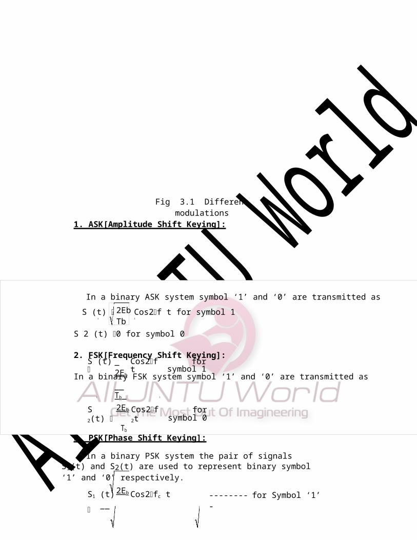
In Binary Huffman Coding each source letter is converted into a binary codeword. It is a prefix condition code ensuring minimum average length per source letter in bits.

Let the source letters a1, a 2, ……….aK have probabilities P(a1), P(a2),………….P(aK) and let us assume that P(a1) ≥ P(a2) ≥ P(a 3)≥…. ≥ P(aK).

We now consider a simple example to illustrate the steps for Huffman coding.

sequence and decode one word at a time. Finding the end of a code word is not a problem

as the present code word is not a prefix to any other codeword.

Example: Consider a coded sequence 0111100 as per Code Representation #3 of

theprevious example. See that the corresponding source letter sequence is a1 ,a4 , a2 , a1 .

Now, we state one important theorem known as Kraft Inequality theorem

withoutproof.

Binary Huffman Coding (an optimum variable-length source coding scheme)

Steps to calculate Huffman Coding

Example Let us consider a discrete memoryless source with six letters having

P(a1)=0.3,P(a2)=0.2, P(a 3)=0.15, P(a 4)=0.15, P(a5)=0.12 and P(a6)=0.08.

Arrange the letters in descending order of their probability (here they are

arranged).

Consider the last two probabilities. Tie up the last two probabilities. Assign, say,

0 to the last digit of representation for the least probable letter (a6) and 1 to the

last digit of representation for the second least probable letter (a5). That is, assign

‘1’ to the upper arm of the tree and ‘0’ to the lower arm.

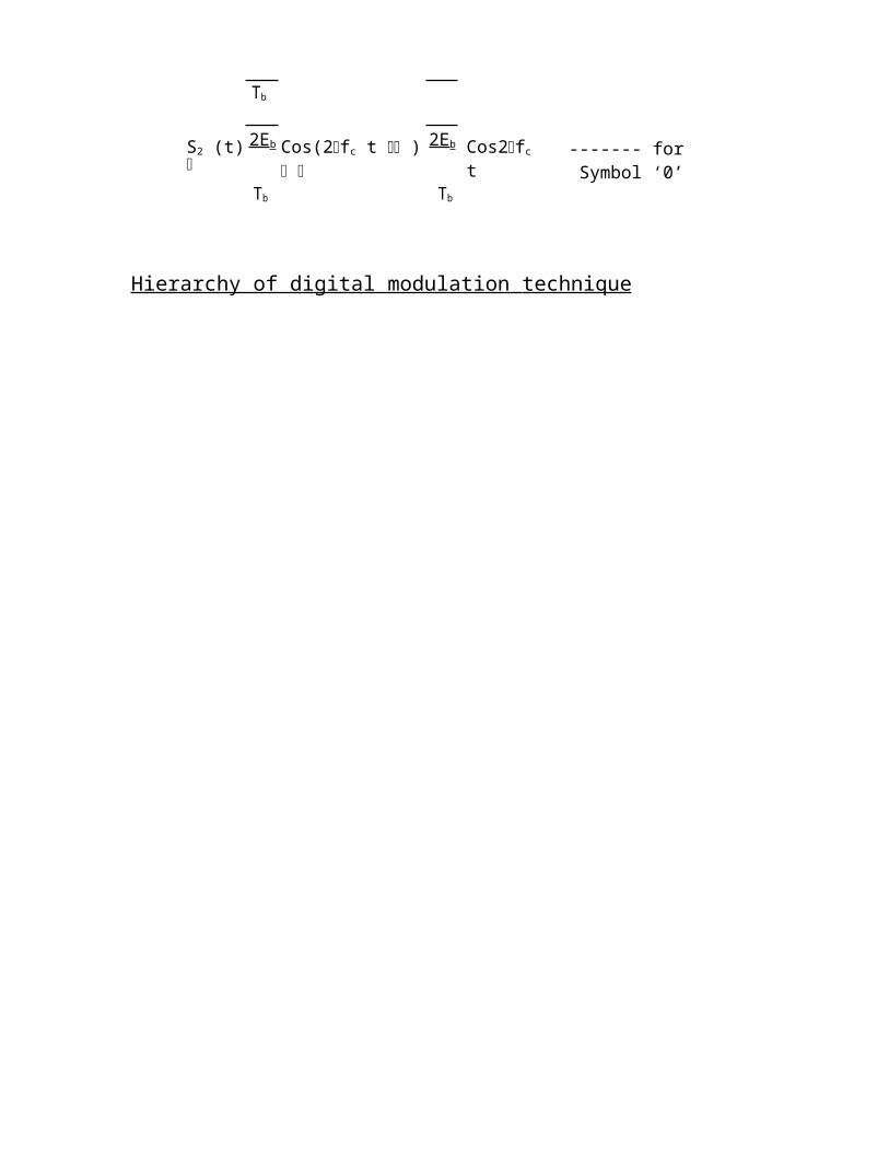
letters. For our example, it leads to:P(a1)=0.3, P(a2)=0.2, P(b1)=0.2, P(a3)=0.15 and P(a4)=0.15

(4) Now go to Step#2 and start with the reduced ensemble consisting of a1 , a2 , a3 ,a4 and b1. Our example results in:

P(a3)=0.15 1

0.3

0

P(a4)=0.15

1

P(a5)=0.12

0.2

P(a6)=0.08 0

(3) Now, add the two probabilities and imagine a new letter, say b1, substituting for

a6 and a5. So P(b1) =0.2. Check whether a4 and b1are the least likely letters. If

not, reorder the letters as per Step#1 and add the probabilities of two least likely

Here we imagine another letter b1, with P(b2)=0.3.

t Continue till the first digits of the most reduced ensemble of two letters are

assigned a ‘1’ and a ‘0’.

Again go back to the step (2): P(a1)=0.3, P(b2)=0.3, P(a2)=0.2 and P(b1)=0.2.

Now we consider the last two probabilities:

P(a2)=0.2

0.4

P(b1)=0.2

P(b2)=0.3 0

with P(b4) = 0.6. Finally we get only two probabilities

P(b4)=0.6 1

1.00

P(b3)=0.40

So, P(b3)=0.4. Following Step#2 again, we get, P(b3)=0.4, P(a1)=0.3 and

P(b2)=0.3.

Next two probabilities lead

to: 1

P(a1)=0.3

0.6

6. Now, read the code tree inward, starting from the root, and construct the

codewords. The first digit of a codeword appears first while reading the code tree

inward.

Hence, the final representation is: a1=11, a2=01, a3=101, a4=100, a5=001, a6=000.

A few observations on the preceding example

1. The event with maximum probability has least number of bits.

2. Prefix condition is satisfied. No representation of one letter is prefix for other.

Prefix condition says that representation of any letter should not be a part of any

other letter.

3. Average length/letter (in bits) after coding is

= ∑P (ai )ni = 2.5 bits/letter.

i

4. Note that the entropy of the source is: H(X)=2.465 bits/symbol. Average length

per source letter after Huffman coding is a little bit more but close to the source

entropy. In fact, the following celebrated theorem due to C. E. Shannon sets the

limiting value of average length of codewords from a DMS.

CONVOLUTIONAL CODES

Convolutional codes are commonly described using two parameters: the code rate and the constraint length. The code rate, k/n, is expressed as a ratio of the number of bits into the convolutional encoder (k) to the number of channel symbols output by the convolutional encoder (n) in a given encoder cycle. The constraint length parameter, K, denotes the "length" of the convolutional encoder, i.e. how many k-bit stages are available to feed the combinatorial logic that produces the output symbols. Closely related to K is the parameter m, which indicates how many encoder cycles an input bit is retained and used for encoding after it first appears at the input to the convolutional encoder. The m parameter can be thought of as the memory length of the encoder.

Convolutional codes are widely used as channel codes in practical communication systems for error correction. The encoded bits depend on the current k input bits and a few past input bits. The main decoding strategy for convolutional codes is based on the widely used Viterbi algorithm. As a result of the wide acceptance of convolutional codes, there have been several approaches to modify and extend this basic coding scheme. Trellis coded modulation (TCM) and turbo codes are two such examples. In TCM, redundancy is added by combining coding and modulation into a single operation. This is achieved without any reduction in data rate or expansion in bandwidth as required by only error correcting coding schemes.

A simple convolutional encoder is shown in Fig. 7.1. The information bits are fed in small groups of k-bits at a time to a shift register. The output encoded bits are obtained by modulo-2 addition (EXCLUSIVE-OR operation) of the input information bits and the contents of the shift registers which are a few previous information bits.

If the encoder generates a group of ‘n’ encoded bits per group of ‘k’ information bits, the code rate R is commonly defined as R = k/n. In Fig. 7.1, k = 1 and n = 2. The number, K of elements in the shift register which decides for how many codewords one information bit will affect the encoder output, is known as the constraint length of the code. For the present example, K = 3.

The shift register of the encoder is initialized to all-zero-state before encoding operation starts. It is easy to verify that encoded sequence is 00 11 10 00 01 ….for an input message sequence of 01011….

Fig. 7.1A convolutional encoder with k=1, n=2 and r=1/2

The operation of a convolutional encoder can be explained in several but equivalent ways such as, by a) state diagram representation, b) tree diagram representation and c) trellis diagram representation.

a) State Diagram Representation

A convolutional encoder may be defined as a finite state machine. Contents of the rightmost (K-1) shift register stages define the states of the encoder. So, the encoder in Fig. 7.2has four states. The transition of an encoder from one state to another, ascaused by input bits, is depicted in the state diagram. Fig. 7.2 shows the state diagram of the encoder in Fig. 7.1. A new input bit causes a transition from one state to another. Thepath information between the states, denoted as b/c1c2 , represents input information bit‘b’ and the corresponding output bits (c1c2). Again, it is not difficult to verify from the state diagram that an input information sequence b = (1011) generates an encoded sequence c = (11, 10, 00, 01).

Fig. 7.2 State diagram representation for the encoder in Fig. 7.1

b)Tree Diagram Representation

The tree diagram representation shows all possible information and encoded sequences for the convolutional encoder. Fig. 7.3 shows the tree diagram for the encoder in Fig. 7.1. The encoded bits are labeled on the branches of the tree. Given an input sequence, the encoded sequence can be directly read from the tree. As an example, an input sequence (1011) results in the encoded sequence (11, 10, 00, 01).

c) Trellis Diagram Representation

The trellis diagram of a convolutional code is obtained from its state diagram. All state transitions at each time step are explicitly shown in the diagram to retain the time dimension, as is present in the corresponding tree diagram. Usually, supporting descriptions on state transitions, corresponding input and output bits etc. are labeled in the trellis diagram. It is interesting to note that the trellis diagram, which describes the operation of the encoder, is very convenient for describing the behavior of thecorresponding decoder, especially when the famous ‘Viterbi Algorithm (VA)’ is followed. Figure 7.4 shows the trellis diagram for the encoder in Figure 7.1.

Fig. 7.3 A tree diagram for the encoder in Fig. 7.1

Fig. 7.4Trellis diagram, used in the decoder corresponding to the encoder in Fig.7.1

The Viterbi algorithm utilizes the trellis diagram to compute the path metrics. The channel is assumed to be memory less, i.e. the noise sample affecting a received bit is independent from the noise sample affecting the other bits. The decoding operation starts from state ‘00’, i.e. with the assumption that the initial state of the encoder is ‘00’. With receipt of one noisy codeword, the decoding operation progresses by one step deeper into the trellis diagram. The branches, associated with a state of the trellis tell us about the corresponding codewords that the encoder may generate starting from this state. Hence, upon receipt of a codeword, it is possible to note the ‘branch metric’ of each branch by determining the Hamming distance of the received codeword from the valid codeword associated with that branch. Path metric of all branches, associated with all the states are calculated similarly Now, at each depth of the trellis, each state also carries some ‘accumulated path metric’, which is the addition of metrics of all branches that construct the ‘most likely path’ to that state. As an example, the trellis diagram of the code shown in Fig. 7.1, has four states and each state has two incoming and two outgoing branches. At any depth of the trellis, each state can be reached through two paths from the previous stage and as per the VA, the path with lower accumulated path metric is chosen. In the

Hard-Decision and Soft-Decision DecodingHard-decision and soft-decision decoding are based on the type of quantization

used on the received bits. Hard-decision decoding uses 1-bit quantization on the received samples. Soft-decision decoding uses multi-bit quantization (e.g. 3 bits/sample) on the received sample values.

Hard-Decision Viterbi AlgorithmThe Viterbi Algorithm (VA) finds a maximum likelihood (ML) estimate of a

transmitted code sequence c from the corresponding received sequence r by maximizing the probability p(r|c) that sequence r is received conditioned on the estimated code sequence c. Sequence c must be a valid coded sequence.

process, the ‘accumulated path metric’ is updated by adding the metric of the incoming branch with the ‘accumulated path metric’ of the state from where the branch originated. No decision about a received codeword is taken from such operations and the decoding decision is deliberately delayed to reduce the possibility of erroneous decision.

The basic operations which are carried out as per the hard-decision Viterbi Algorithm after receiving one codeword are summarized below:

All the branch metrics of all the states are determined;

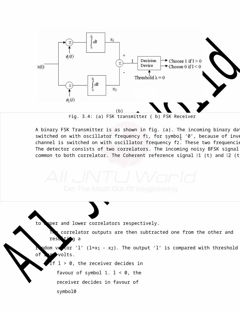
(5) Steps a) to d) are repeated and decoding decision is delayed till sufficient number of codewords has been received. Typically, the delay in decision making = Lx k codewords where L is an integer, e.g. 5 or 6. For the code in Fig. 7.1, the decision delay of 5x3 = 15 codewords may be sufficient for most occasions. This means, we decide about the first received codeword after receiving the 16thcodeword. The decision strategy is simple. Upon receiving the 16thcodeword and carrying out steps a) to d), we compare the ‘accumulated path metrics’ of all the states ( four in our example) and chose the state with minimum overall ‘accumulated path metric’ as the ‘winning node’ for the first codeword. Then we trace back the history of the path associated with this winning node to identify the codeword tagged to the first branch of the path and declare this codeword as the most likely transmitted first codeword.The above procedure is repeated for each received codeword hereafter. Thus, the decision for a codeword is delayed but once the decision process starts, we decide once for every received codeword. For most practical applications, including delay-sensitive digital speech coding and transmission, a decision delay of Lx k codewords is acceptable.

.

Accumulated metrics of all the paths (two in our example code) leading to a state are calculated taking into consideration the ‘accumulated path metrics’ of the states from where the most recent branches emerged;

Only one of the paths, entering into a state, which has minimum ‘accumulated path metric’ is chosen as the ‘survivor path’ for the state (or, equivalently ‘node’);

So, at the end of this process, each state has one ‘survivor path’. The ‘history’ of a survivor path is also maintained by the node appropriately ( e.g. by storing the codewords or the information bits which are associated with the branches making the path);

Soft-Decision Viterbi AlgorithmIn soft-decision decoding, the demodulator does not assign a ‘0’ or a ‘1’ to

each received bit but uses multi-bit quantized values. The soft-decision Viterbi algorithm is very similar to its hard-decision algorithm except that squared Euclidean distance is used in the branch metrics instead of simpler Hamming distance. However, the performance of a soft-decision VA is much more impressive compared to its HDD (Hard Decision Decoding) counterpart [Fig. 7.6 (a) and (b)]. The computational requirement of a Viterbi decoder grows exponentially as a function of the constraint length and hence it is usually limited in practice to constraint lengths of K = 9.

Fig. 7.6 (a) Decoded BER vs input BER for the rate – half convolutional codes withViterbi Algorithm ; 1) k = 3 (HDD),2) k = 5 (HDD),3) k = 3 (SDD), and 4) k= 5 (SDD). HDD: Hard Decision Decoding; SDD: Soft Decision Decoding.

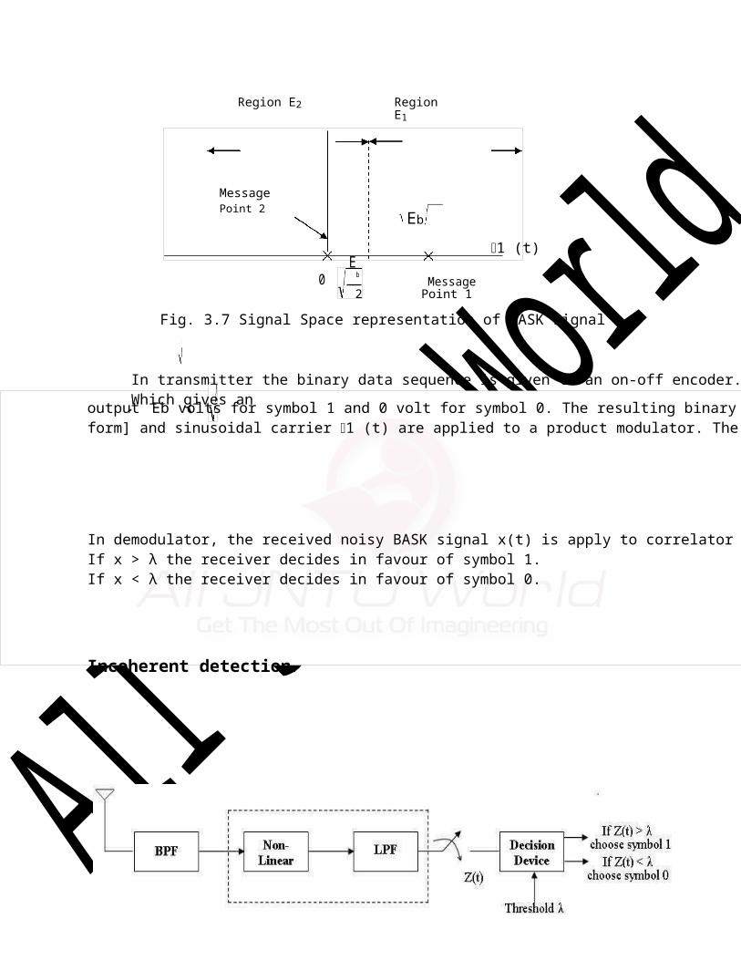
Fig. 7.6 (b) Decoded BER vs Eb/No(in dB) for the rate – half convolutional codes withViterbi Algorithm ; 1) Uncoded system; 2) with k = 3 (HDD) and 3) k = 3 (SDD). HDD: Hard Decision Decoding; SDD: Soft Decision Decoding.

Spread – Spectrum Modulation

Introduction:

Initially developed for military applications during II world war, that was less sensitive to intentional interference or jamming by third parties.

Spread spectrum technology has blossomed into one of the fundamental building blocks in current and next-generation wireless systems

Problem of radio transmission

Narrow band can be wiped out due to interference

To disrupt the communication, the adversary needs to do two things,

to detect that a transmission is taking place and

to transmit a jamming signal which is designed to confuse the receiver.

Solution

A spread spectrum system is therefore designed to make these tasks as difficult as possible.

Firstly, the transmitted signal should be difficult to detect by an adversary/jammer, i.e.,the signal should have a low probability of intercept (LPI).

Secondly, the signal should be difficult to disturb with a jamming signal, i.e., thetransmitted signal should possess an anti-jamming (AJ) property

Remedy

Spread the narrow band signal into a broad band to protect against interference

In a digital communication system the primary resources are Bandwidth andPower. The study of digital communication system deals with efficient utilization ofthese two resources, but there are situations where it is necessary to sacrifice their efficient utilization in order to meet certain other design objectives.

For example to provide a form of secure communication (i.e. the transmitted signal is not easily detected or recognized by unwanted listeners) the bandwidth of thetransmitted signal is increased in excess of the minimum bandwidth necessary to transmit it. This requirement is catered by a technique known as “Spread SpectrumModulation”.

The primary advantage of a Spread – Spectrum communication system is its ability to reject ‘Interference’ whether it be the unintentional or the intentionalinterference.

The definition of Spread – Spectrum modulation may be stated in two parts.

Spread Spectrum is a mean of transmission in which the data sequence occupies a BW (Bandwidth) in excess of the minimum BW necessary to transmit it.

The Spectrum Spreading is accomplished before transmission through the use of a code that is independent of the data sequence. The Same code is used in the receiver to despread the received signal so that the original data sequence may be recovered.

s(t) wide band r(t) wide band b(t) + Noise

Bandb(t) . . . . . . . . . Narrow Wide

Band

c(t) n(t) c(t)

Wide band (noise) Wide band

---- Transmitter---- ---- Channel------ --- Receiver--------

Fig: 8.1 spread spectrum technique.

b(t) = Data Sequence to be transmitted (Narrow Band) c(t)= Wide Band codes(t) = c(t) * b(t) – (wide Band)

Fig: 8.2Spectrum of signal before & after spreading

Code division multiple access

CDMA is achannel access methodutilized by various radio communication technologies.

One of the basic concepts in data communication is the idea of allowing several transmitters to send information simultaneously over a single communication channel. This allows several users to share a bandwidth of frequencies. This concept is called multiplexing. CDMA employs spread-spectrum technology and a special coding scheme (where each transmitter is assigned a code) to allow multiple users to be multiplexed over the same physical channel. By contrast, time division multiple access (TDMA) divides access by time, while frequency-division multiple access (FDMA) divides it by frequency. CDMA is a form of "spread-spectrum" signaling, since the modulated coded signal has a much higher data bandwidth than the data being communicated.

An analogy to the problem of multiple access is a room (channel) in which people wish to communicate with each other. To avoid confusion, people could take turns speaking (time division), speak at different pitches (frequency division), or speak in different languages (code division). CDMA is analogous to the last example where people speaking the same language can understand each other, but not other people. Similarly, in radio CDMA, each group of users is given a shared code. Many codes occupy the same channel, but only users associated with a particular code can understand each other.

Technical details

CDMA is a spread spectrum multiple access technique. In CDMA a locally generated code runs at a much higher rate than the data to be transmitted. Data for transmission is simply logically XOR (exclusive OR) added with the faster code. The figure shows how spread spectrum signal is generated. The data signal with pulse duration of Tb is XOR added with the code signal with pulse duration of Tc. (Note: bandwidth is proportional to 1 / T where T = bit time) Therefore, the bandwidth of the data signal is 1 / Tb and the bandwidth of the spread spectrum signal is 1 / Tc. Since Tc is much smaller than Tb, the bandwidth of the spread spectrum signal is much larger than the bandwidth of the original signal.

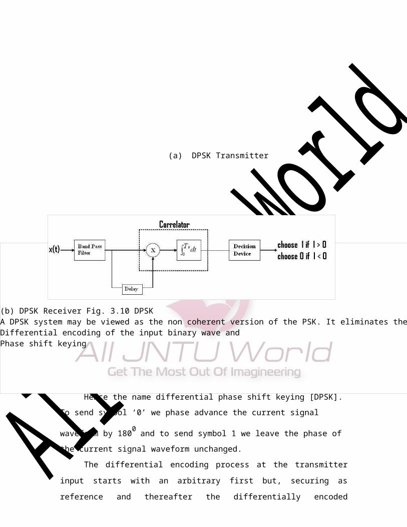
Fig. 8.3

CDMA uses Direct Sequence spreading, where spreading process isdone by directly combining the baseband information to high chip rate binary code. The Spreading Factor is the ratio of the chips (UMTS = 3.84Mchips/s) to baseband information rate. Spreading factors vary from 4 to 512 in FDD UMTS. Spreading process gain can in expressed in dBs (Spreading factor 128 = 21dB gain).

Fig. 8.4

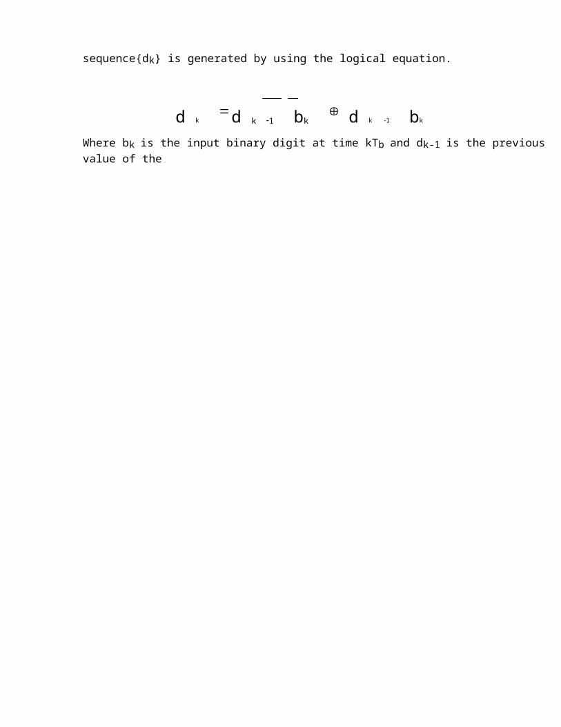
Each user in a CDMA system uses a different code to modulate their signal. Choosing the codes used to modulate the signal is very important in the performance of CDMA systems. The best performance will occur when there is good separation between the signal of a desired user and the signals of other users. The separation of the signals is made by correlating the received signal with the locally generated code of the desired user. If the signal matches the desired user's code then the correlation function will be high and the system can extract that signal. If the desired user's code has nothing in common with the signal the correlation should be as close to zero as possible (thus eliminating the signal); this is referred to as cross correlation. If the code is correlated with the signal at any time offset other than zero, the correlation should be as close to zero as possible. This is referred to as auto-correlation and is used to reject multi-path interference.

Fig. 8.5

Fig 8.6: Maximum-length sequence generator for n=3

A feedback shift register is said to be Linear when the feed back logic consists of entirely mod-2-address ( Ex-or gates). In such a case, the zero state is not permitted. The period of a PN sequence produced by a linear feedback shift register with ‘n’ flip flops cannot exceed 2n-1. When the period is exactly 2n-1, the PN sequence is called a‘maximum length sequence’ or ‘m-sequence’.

Example1: Consider the linear feed back shift register as shown in fig 2involvethree flip-flops. The input so is equal to the mod-2 sum of S1 and S3. If the initial state of the shift register is 100. Then the succession of states will be as follows.

PSUEDO-NOISE SEQUENCE:

Generation of PN sequence:

Clock

Shift Shift Shift Output

S0Register1 Register2 S3

Register3

Logic Circuit

100,110,011,011,101,010,001,100 . . . . . .

The output sequence (output S3) is therefore. 00111010 . . . . .

Which repeats itself with period 23–1 = 7 (n=3)

Maximal length codes are commonly used PN codes

In binary shift register, the maximum length sequence is

N = 2m-1

chips, where m is the number of stages of flip-flops in the shift register.

Fig. 8.8 Initial stages of Shift registers1000 Let initial status of shift register be 1000

Fig.8.7

At each clock pulse

(6) Contents of register shifts one bit right.

(7) Contents of required stages are modulo 2 added and fed back to input.

1 0 0 00 1 0 00 0 1 01 0 0 11 1 0 00 1 1 01 0 1 10 1 0 11 0 1 01 1 0 11 1 1 01 1 1 10 1 1 10 0 1 10 0 0 11 0 0 0

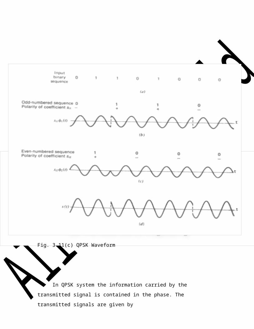
• We can see for shift Register of length m=4.

.At each clock the change in state of flip-flop is shown.

•Feed back function is modulo two of X3andX4.

•After 15 clock pulses the sequence repeats. Output sequence is

0 0 0 1 0 0 1 1 0 1 0 1 1 1 1

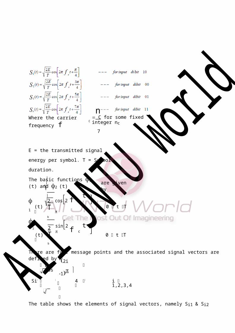
Properties of PN SequenceRandomness of PN sequence is tested by following properties

u Balance propertyv Run length propertyw Autocorrelation property

1. Balance property

In each Period of the sequence , number of binary ones differ from binary zeros by at most one digit .Consider output of shift register 0 0 0 1 0 0 1 1 0 1 0 1 1 1 1 Seven zeros and eight ones -meets balance condition.

2. Run length property

Among the runs of ones and zeros in each period, it is desirable that about one half the runs of each type are of length 1, one- fourth are of length 2 and one-eighth are of length 3 and so- on.

Consider output of shift register Number of runs =8

0 0 0 1 0 0 1 1 0 1 01 1 1 13 1 2 2 1 1 1 4

{ No. of agreements – No. of disagreements in comparison of one full period } Consider output of shift register for l=1

Yields PN autocorrelation as

Range of PN Sequence Lengths

Length 0f Shift Register, m PN Sequence Length,

7 127

8 255

9 511

10 1023

11 2047

12 4095

13 8191

17 13107119 524287

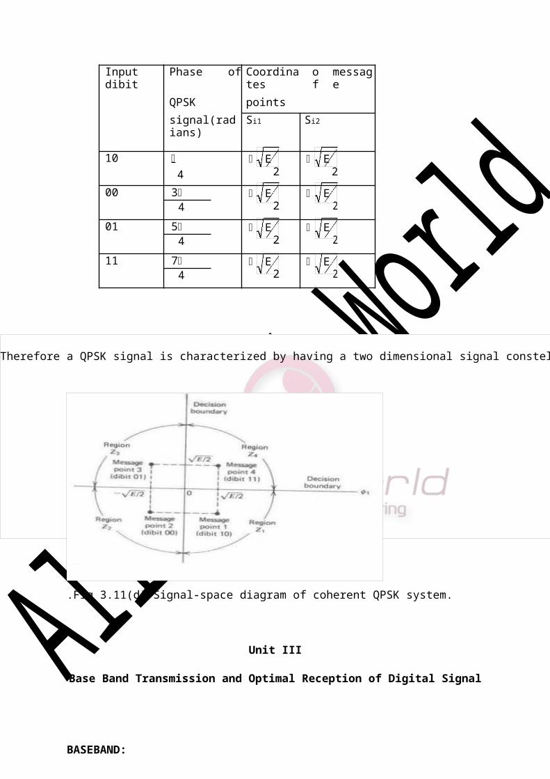
b(t) m(t). . r(t) z(t) Decisi on Device

0dt

Tb

<----Transmitter-----> --Channel - - - - - Receiver -------------

Let { bK} denotes a binary data sequence.

{ cK } denotes a PN sequence.

b(t) and c(t) denotes their NRZ polar representation respectively.

The desired modulation is achieved by applying the data signal b(t) and PN signal c(t) to a product modulator or multiplier. If the message signal b(t) is narrowband and the PN sequence signal c(t) is wide band, the product signal m(t) is also wide band. The PN

sequence performs the role of a ‘Spreading Code”.

A Notion of Spread Spectrum:

An important attribute of Spread Spectrum modulation is that it can provide protection against externally generated interfacing signals with finite power. Protection against jamming (interfacing) waveforms is provided by purposely making the information– bearing signal occupy a BW far in excess of the minimum BW necessary to transmit it. This has the effect of making the transmitted signal a noise like appearance so as to blend into the background. Therefore Spread Spectrum is a method of ‘camouflaging’ the information – bearing signal.

V

c(t) n(t) c(t) Threshold=0

For base band transmission, the product signal m(t) represents the transmitted

signal. Therefore m(t) = c(t).b(t)

The received signal r(t) consists of the transmitted signal m(t) plus an additive interference noise n(t), Hence

r(t) = m(t) + n(t)

= c(t).b(t) + n(t)

+1

0

-1

a) Data Signal b(t)

+1

0 -1

1

0 -1

b)Spreading Code c(t)

+

c)Product signal or base band transmitted signal m(t)

To recover the original message signal b(t), the received signal r(t) is applied to a demodulator that consists of a multiplier followed by an integrator and a decision device. The multiplier is supplied with a locally generated PN sequence that is exact replica of that used in the transmitter. The multiplier output is given by

Z(t) = r(t).c(t)

4.[b(t) * c(t) + n(t)] c(t)

5.c2(t).b(t) + c(t).n(t)

The data signal b(t) is multiplied twice by the PN signal c(t), where as unwanted signal n(t) is multiplied only once. But c2(t) = 1, hence the above equation reduces to

Z(t) = b(t) + c(t).n(t)

Now the data component b(t) is narrowband, where as the spurious component c(t)n(t) is wide band. Hence by applying the multiplier output to a base band (low pass) filter most of the power in the spurious component c(t)n(t) is filtered out. Thus the effect of the interference n(t) is thus significantly reduced at the receiver output.

The integration is carried out for the bit interval 0 ≤ t ≤ Tb to provide the sample value V. Finally, a decision is made by the receiver.

If V > Threshold Value ‘0’, say binary symbol ‘1’

If V < Threshold Value ‘0’, say binary symbol ‘0’

Frequency – Hop Spread Spectrum:

In a frequency – hop Spread – Spectrum technique, the spectrum of data modulated carrier is widened by changing the carrier frequency in a pseudo – random manner. The type of spread – spectrum in which the carrier hops randomly form one frequency to another is called Frequency–Hop (FH) Spread Spectrum.

Since frequency hopping does not covers the entire spread spectrum instantaneously. We are led to consider the rate at which the hop occurs. Depending upon this we have two types of frequency hop.

1. Slow frequency hopping:- In which the symbol rate Rs of the MFSK signal is aninteger multiple of the hop rate Rh. That is several symbols are transmitted on each frequency hop.

2. Fast – Frequency hopping:- In which the hop rate Rh is an integral multiple of theMFSK symbol rate Rs. That is the carrier frequency will hoop several times during the transmission of one symbol.

A common modulation format for frequency hopping system is that of M- ary frequency – shift – keying (MFSK).

Slow frequency hopping:-

Fig. 8.12 a) Shows the block diagram of an FH / MFSK transmitter, which involves

frequency modulation followed by mixing.

The incoming binary data are applied to an M-ary FSK modulator. The resulting modulated wave and the output from a digital frequency synthesizer are then applied to a mixer that consists of a multiplier followed by a band – pass filter. The filter is designed

to select the sum frequency component resulting from the multiplication process as the transmitted signal. An ‘k’ bit segments of a PN sequence drive the frequencysynthesizer, which enables the carrier frequency to hop over 2n distinct values. Since frequency synthesizers are unable to maintain phase coherence over successive hops, most frequency hops spread spectrum communication system use non coherent M-ary modulation system.

Fig 8.12:- Frequency hop spread M-ary Frequency – shift – keying

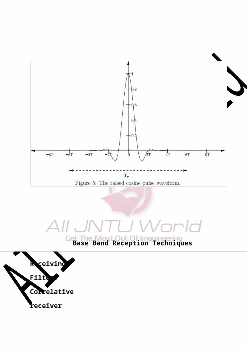
Where Rh is the hop rate and Rs is Symbol Rate

In a slow rate frequency hopping multiple symbols are transmitted per hop. Henceeach symbol of a slow FH / MFSK signal is a chip. The bit rate Rb of theincoming binarydata. The symbol rate Rs of the MFSK signal, the chip rate Rc and the hop rate Rn are related by

Rc = Rs = Rb /k ≥ Rh

where k= log2M

In the receiver the frequency hoping is first removed by mixing the received signal with the output of a local frequency synthesizer that is synchronized with the transmitter. The resulting output is then band pass filtered and subsequently processed by a non coherent M- ary FSK demodulator. To implement this M-ary detector, a bank of M non coherent matched filters, each of which is matched to one of the MFSK tones is used. By selecting the largest filtered output, the original transmitted signal is estimated.

An individual FH / MFSK tone of shortest duration is referred as a chip. The chip rate Rc for an FH / MFSK system is defined by

Rc = Max(Rh,Rs)

Fast frequency hopping:-

A fast FH / MFSK system differs from a slow FH / MFSK system in that there are multiple hops per m-ary symbol. Hence in a fast FH / MFSK system each hop is a chip.

Fig. illustrates the variation of the frequency of a slow FH/MFSK signal with time for one complete period of the PN sequence. The period of the PN sequence is 24-1 = 15. The FH/MFSK signal has the following parameters:

Number of bits per MFSK symbol K = 2.

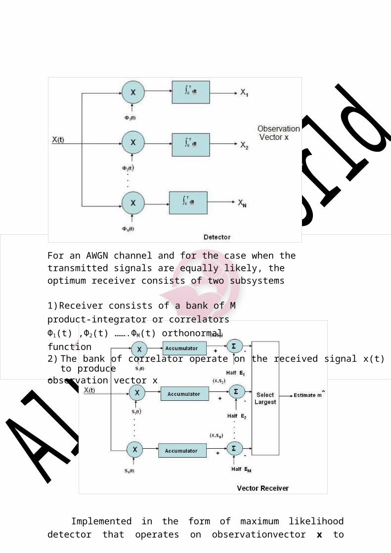
Number of MFSK tones M = 2K = 4

Length of PN segment per hop k = 3

Total number of frequency hops 2k = 8

Fig. illustrates the variation of the transmitted frequency of a fast FH/MFSK signal with time. The signal has the following parameters:

Number of bits per MFSK symbol K = 2.

Number of MFSK tones M = 2K = 4

Length of PN segment per hop k = 3

Total number of frequency hops 2k = 8