Lecture Notes Computer Graphics

Prepared By- Ipsita Panda

Sem-7th

Branch-CSE

Sub code-PCCS4401

Module-I

Computer graphicsComputer graphics remains one of the most existing and rapidly growing computer fields. Computer graphics may be defined as a pictorial representation or graphical representation of objects in a computer.

Application of Computer Graphics

Computer-Aided Design

Computer-Aided Design for engineering and architectural systems etc. Objects maybe displayed in a wireframe outline form. Multi-window environment is also favored for producing various zooming scales and views. Animations are useful for testing performance.

Presentation Graphics

To produce illustrations which summarize various kinds of data. Except 2D, 3D graphics are good tools for reporting more complex data.

Computer Art

Painting packages are available. With cordless, pressure-sensitive stylus, artists can produce electronic paintings which simulate different brush strokes, brush widths, and colors. Photorealistic techniques, morphing and animations are very useful in commercial art. For films, 24 frames per second are required. For video monitor, 30 frames per second are required.

Entertainment

Motion pictures, Music videos, and TV shows, Computer games

Education and Training

Training with computer-generated models of specialized systems such as the training of ship captains and aircraft pilots.

Visualization

For analyzing scientific, engineering, medical and business data or behavior. Converting data to visual form can help to understand mass volume of data very efficiently.

Image Processing

Image processing is to apply techniques to modify or interpret existing pictures. It is widely used in medical applications.

Graphical User Interface

Multiple window, icons, menus allow a computer setup to be utilized more efficiently.

Overview of Graphics Systems

Cathode-Ray Tubes (CRT) –

Still the most common video display device presently electrostatic deflection of the electron beam in a CRT. An electron gun emits a beam of electrons, which passes through focusing and deflection systems and hits on the phosphor-coated screen. A beam of electrons (cathode rays), emitted by an electron gun, passes through focusing and deflection systems that direct the beam towards specified position on the phosphor-coated screen. The phosphor then emits a small spot of light at each position contacted by the electron beam. Because the light emitted by the phosphor fades very rapidly, some method is needed for maintaining the screen picture. One way to keep the phosphor glowing is to redraw the picture repeatedly by quickly directing the electron beam back over the same points. This type of display is called a refresh CRT.

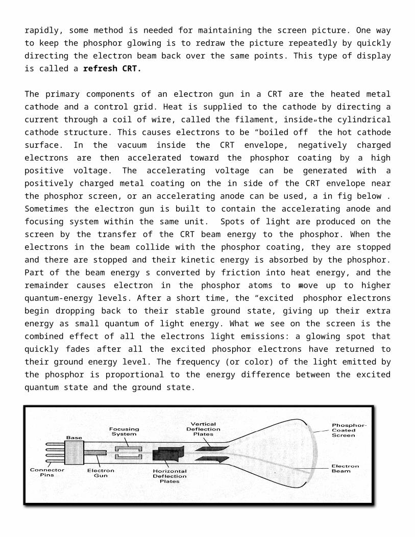
The primary components of an electron gun in a CRT are the heated metal cathode and a control grid. Heat is supplied to the cathode by directing a current through a coil of wire, called the filament, inside the cylindrical cathode structure. This causes electrons to be “boiled off” the hot cathode surface. In the vacuum inside the CRT envelope, negatively charged electrons are then accelerated toward the phosphor coating by a high positive voltage. The accelerating voltage can be generated with a positively charged metal coating on the in side of the CRT envelope near the phosphor screen, or an accelerating anode can be used, a in fig below . Sometimes the electron gun is built to contain the accelerating anode and focusing system within the same unit. Spots of light are produced on the screen by the transfer of the CRT beam energy to the phosphor. When the electrons in the beam collide with the phosphor coating, they are stopped and there are stopped and their kinetic energy is absorbed by the phosphor. Part of the beam energy s converted by friction into heat energy, and the remainder causes electron in the phosphor atoms to move up to higher quantum-energy levels. After a short time, the “excited” phosphor electrons begin dropping back to their stable ground state, giving up their extra energy as small quantum of light energy. What we see on the screen is the combined effect of all the electrons light emissions: a glowing spot that quickly fades after all the excited phosphor electrons have returned to their ground energy level. The frequency (or color) of the light emitted by the phosphor is proportional to the energy difference between the excited quantum state and the ground state.

Different kinds of phosphor are available for use in a CRT. Besides color, a major difference between phosphors is their persistence: how long they continue to emit light (that is, have excited electrons returning to the ground state) after the CRT beam is removed. Persistence is defined as the time it takes the emitted light from the screen to decay to one-tenth of its original intensity. Lower-persistence phosphors require higher refresh rates to maintain a picture on the screen without flicker. A phosphor with low persistence is useful for animation; a high-persistence phosphor is useful for displaying highly complex, static pictures. Although some phosphor have a persistence greater than 1 second, graphics monitor are usually constructed with a persistence in the range from 10 to 60 microseconds

Raster-scan technique

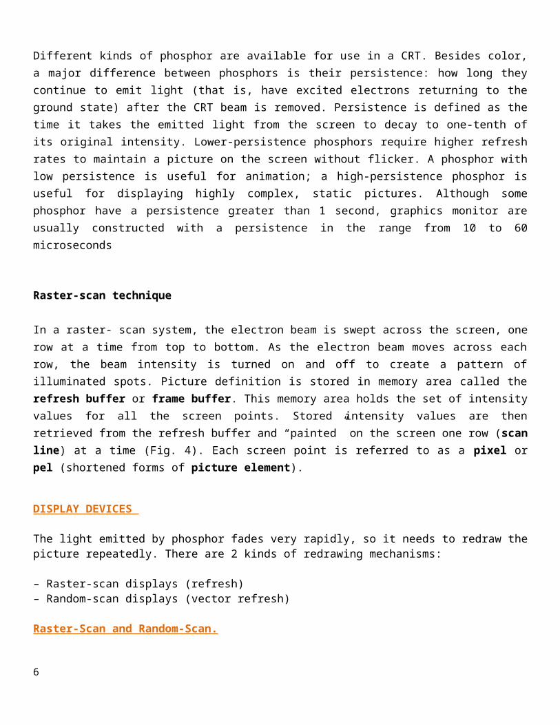
In a raster- scan system, the electron beam is swept across the screen, one row at a time from top to bottom. As the electron beam moves across each row, the beam intensity is turned on and off to create a pattern of illuminated spots. Picture definition is stored in memory area called the refresh buffer or frame buffer. This memory area holds the set of intensity values for all the screen points. Stored intensity values are then retrieved from the refresh buffer and “painted” on the screen one row (scan line) at a time (Fig. 4). Each screen point is referred to as a pixel or pel (shortened forms of picture element).

DISPLAY DEVICES

The light emitted by phosphor fades very rapidly, so it needs to redraw the picture repeatedly. There are 2 kinds of redrawing mechanisms:

– Raster-scan displays (refresh) – Random-scan displays (vector refresh)

Raster-Scan and Random-Scan.

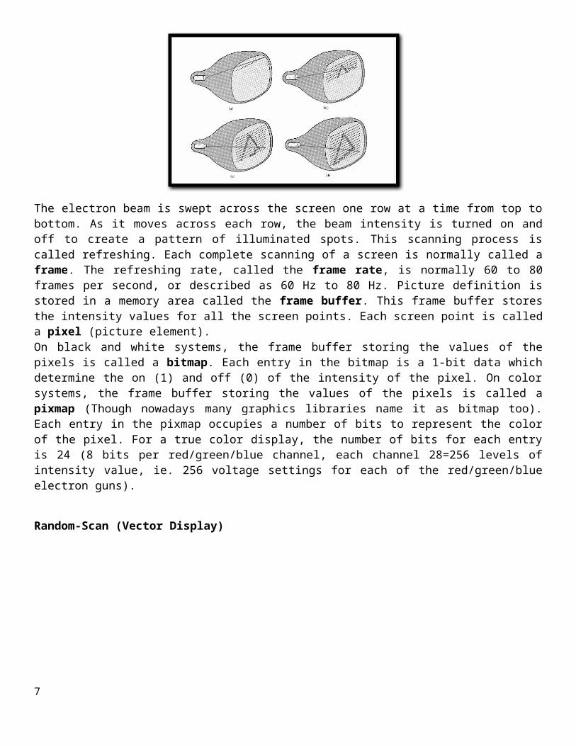
The electron beam is swept across the screen one row at a time from top to bottom. As it moves across each row, the beam intensity is turned on and off to create a pattern of illuminated spots. This scanning process is called refreshing. Each complete scanning of a screen is normally called a frame. The refreshing rate, called the

5

frame rate, is normally 60 to 80 frames per second, or described as 60 Hz to 80 Hz. Picture definition is stored in a memory area called the frame buffer. This frame buffer stores the intensity values for all the screen points. Each screen point is called a pixel (picture element).On black and white systems, the frame buffer storing the values of the pixels is called a bitmap. Each entry in the bitmap is a 1-bit data which determine the on (1) and off (0) of the intensity of the pixel. On color systems, the frame buffer storing the values of the pixels is called a pixmap (Though nowadays many graphics libraries name it as bitmap too). Each entry in the pixmap occupies a number of bits to represent the color of the pixel. For a true color display, the number of bits for each entry is 24 (8 bits per red/green/blue channel, each channel 28=256 levels of intensity value, ie. 256 voltage settings for each of the red/green/blue electron guns).

Random-Scan (Vector Display)

The CRT's electron beam is directed only to the parts of the screen where a picture is to be drawn.The picture definition is stored as a set of line-drawing commands in a refresh display file or a refresh buffer in memory. Random-scan generally have higher resolution than raster systems and can produce smooth line drawings, however it cannot display realistic shaded scenes.

6

Graphics Systems

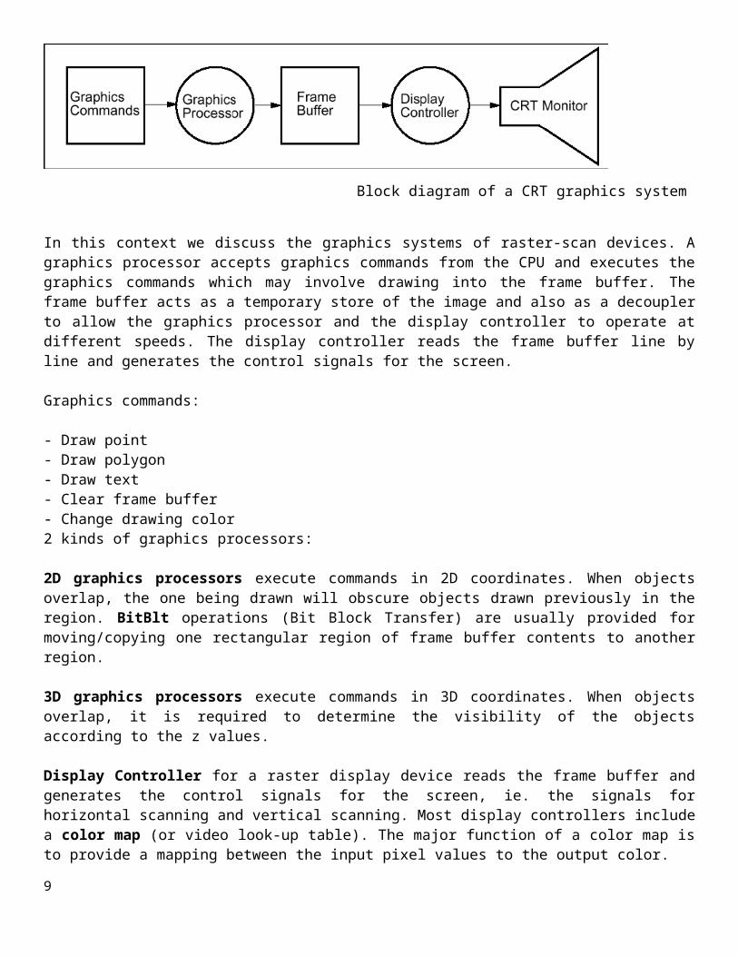
Block diagram of a CRT graphics system

In this context we discuss the graphics systems of raster-scan devices. A graphics processor accepts graphics commands from the CPU and executes the graphics commands which may involve drawing into the frame buffer. The frame buffer acts as a temporary store of the image and also as a decoupler to allow the graphics processor and the display controller to operate at different speeds. The display controller reads the frame buffer line by line and generates the control signals for the screen.

Graphics commands:

- Draw point- Draw polygon- Draw text- Clear frame buffer- Change drawing color2 kinds of graphics processors:

2D graphics processors execute commands in 2D coordinates. When objects overlap, the one being drawn will obscure objects drawn previously in the region. BitBlt operations (Bit Block Transfer) are usually provided for moving/copying one rectangular region of frame buffer contents to another region.

3D graphics processors execute commands in 3D coordinates. When objects overlap, it is required to determine the visibility of the objects according to the z values.

Display Controller for a raster display device reads the frame buffer and generates the control signals for the screen, ie. the signals for horizontal scanning and vertical scanning. Most display controllers include a color map (or video look-up table). The major function of a color map is to provide a mapping between the input pixel values to the output color.

7

Color CRT monitor

The beam penetration method for displaying color pictures has been used with random-scan monitors. Two layers of phosphor, usually red and green, are coated on to theinside of the CRT screen, and the displayed color depends on how far the electron beam penetrates into the phosphor layers.

Shadow-mask

Shadow-mask methods are commonly used in raster-scan systems (including color TV) because they produce a much wider range of color than the beam penetration method. A shadow-mask CRT has three phosphor color dots at each pixel position. One phosphor dot emits a red light, another emits a green light, and the third emits a blue light. This type of CRT has three electron guns, one for each color dot, and a shadow- mask grid just behind the phosphor –coated screen. Figure 6 below illustrates the delta-delta shadow-mask method, commonly used in color CRT systems. The three electron beam are deflected and focused as a group onto the shadow mask, which contains a series of holes aligned with the phosphor-dot patterns. When the three beams pass through a hole in the shadow mask, they activate a dot triangle, which appears as a small color spot the screen the phosphor dots in the triangles are arranged so that each electron beam can activate only its corresponding color dot when it passes through the shadow mask .

8

Input Devices

Common devices: keyboard, mouse, trackball and joystick Specialized devices:

Data gloves are electronic gloves for detecting fingers' movement. In some applications, a sensor is also attached to the glove to detect the hand movement as a whole in 3D space.A tablet contains a stylus and a drawing surface and it is mainly used for the input of drawings. A tablet is usually more accurate than a mouse, and is commonly used for large drawings.Scanners are used to convert drawings or pictures in hardcopy format into digital signal for computer processing.Touch panels allow displayed objects or screen positions to be selected with the touch of a finger. In these devices a touch-sensing mechanism is fitted over the video monitor screen. Touch input can be recorded using optical, electrical, or acoustical methods.

Hard-Copy DevicesDirecting pictures to a printer or plotter to produce hard-copy output on 35-mm slides, overhead transparencies, or plain paper. The quality of the pictures depends on dot size and number of dots per inch (DPI).Types of printers: line printers, laserjet, ink-jet, dot-matrix

Laserjet printers use a laser beam to create a charge distribution on a rotating drum coated with a photoelectric material. Toner is applied to the drum and then transferred to the paper. To produce color outputs, the 3 color pigments (cyan, magenta, and yellow) are deposited on separate passes.

Inkjet printers produce output by squirting ink in horizontal rows across a roll of paper wrapped on a drum. To produce color outputs, the 3 color pigments are shot simultaneously on a single pass along each print line on the paper.Inkjet or pen plotters are used to generate drafting layouts and other drawings of normally larger sizes. A pen plotter has one or more pens of different colors and widths mounted on a carriage which spans a sheet of paper.

9

Coordinate Representations in Graphics

General graphics packages are designed to be used with Cartesian coordinate representations (x,y,z).Usually several different Cartesian reference frames are used to construct and display a scene:

Modeling coordinates are used to construct individual object shapes.

World coordinates are computed for specifying the placement of individual objects in appropriatepositions.

Normalized coordinates are converted from world coordinates, such that x,y values are ranged from 0 to 1.

Device coordinates are the final locations on the output devices.

10

Output Primitives

Drawing a Thin Line in Raster Devices

This is to compute intermediate discrete coordinates along the line path between 2 specified endpoint positions. The corresponding entry of these discrete coordinates in the frame buffer is then marked with the line color wanted.

The basic concept is:

A line can be specified in the form: y = mx + c

Let m be between 0 to 1, then the slope of the line is between 0 and 45 degrees.

For the x-coordinate of the left end point of the line, compute the corresponding y value according to the line equation. Thus we get the left end point as (x1,y1), where y1 may not be an integer.

Calculate the distance of (x1,y1) from the center of the pixel immediately above it and call it D1

Calculate the distance of (x1,y1) from the center of the pixel immediately below it and call it D2

If D1 is smaller than D2, it means that the line is closer to the upper pixel than the lower pixel, then, we set the upper pixel to on; otherwise we set the lower pixel to on.

Then increatement x by 1 and repeat the same process until x reaches the right end point of the line.

This method assumes the width of the line to be zero.

Digital differential analyzer(DDA)

In computer graphics, a hardware or software implementation of a digital differential analyzer (DDA) is used for linear interpolation of variables over an interval between start and end point. DDAs are used for rasterization of lines, triangles and polygons.

The DDA method can be implemented using floating-point or integer arithmetic. The native floating-point implementation requires one addition and one rounding operation per interpolated value (e.g. coordinate x, y, depth, color component etc.) and output result. This process is only efficient when an FPU with fast add and rounding operation is available.

The fixed-point integer operation requires two additions per output cycle, and in case of fractional part overflow, one additional increment and subtraction. The probability of fractional part overflows is proportional to the ratio m of the interpolated start/end values.

11

DDAs are well suited for hardware implementation and can be pipelined for maximized throughput.

Where m represents the slope of the line and c is the y intercept . this slope can be expressed in DDA as

in fact any two consecutive point(x,y) laying on this line segment should satisfy the equation.

The DDA starts by calculating the smaller of dy or dx for a unit increment of the other. A line is then sampled at unit intervals in one coordinate and corresponding integer values nearest the line path are determined for the other coordinate.

Considering a line with positive slope, if the slope is less than or equal to 1, we sample at unit x intervals (dx=1) and compute successive y values as

Subscript k takes integer values starting from 0, for the 1st point and increases by 1 until endpoint is reached. y value is rounded off to nearest integer to correspond to a screen pixel.

For lines with slope greater than 1, we reverse the role of x and y i.e. we sample at dy=1 and calculate consecutive x values as

Similar calculations are carried out to determine pixel positions along a line with negative slope. Thus, if the absolute value of the slope is less than 1, we set dx=1 if i.e. the starting extreme point is at the left.

Algorithm:-

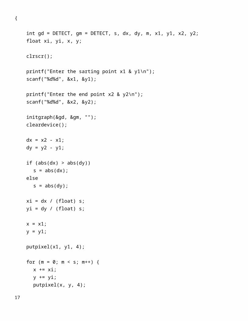
#include <graphics.h>#include <stdio.h>#include <conio.h>#include <math.h> void main(){  int gd = DETECT, gm = DETECT, s, dx, dy, m, x1, y1, x2, y2; float xi, yi, x, y;

12

  clrscr();  printf("Enter the sarting point x1 & y1\n"); scanf("%d%d", &x1, &y1);  printf("Enter the end point x2 & y2\n"); scanf("%d%d", &x2, &y2);  initgraph(&gd, &gm, ""); cleardevice();  dx = x2 - x1; dy = y2 - y1;  if (abs(dx) > abs(dy))

s = abs(dx); else

s = abs(dy);  xi = dx / (float) s; yi = dy / (float) s;  x = x1; y = y1;  putpixel(x1, y1, 4);  for (m = 0; m < s; m++) {

x += xi;y += yi;putpixel(x, y, 4);

} getch();}

13

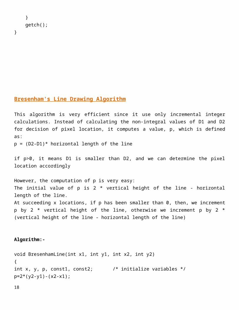
Bresenham's Line Drawing Algorithm

This algorithm is very efficient since it use only incremental integer calculations. Instead of calculating the non-integral values of D1 and D2 for decision of pixel location, it computes a value, p, which is defined as:p = (D2-D1)* horizontal length of the line

if p>0, it means D1 is smaller than D2, and we can determine the pixel location accordingly

However, the computation of p is very easy:The initial value of p is 2 * vertical height of the line - horizontal length of the line.At succeeding x locations, if p has been smaller than 0, then, we increment p by 2 * vertical height of the line, otherwise we increment p by 2 * (vertical height of the line - horizontal length of the line)

Algorithm:-

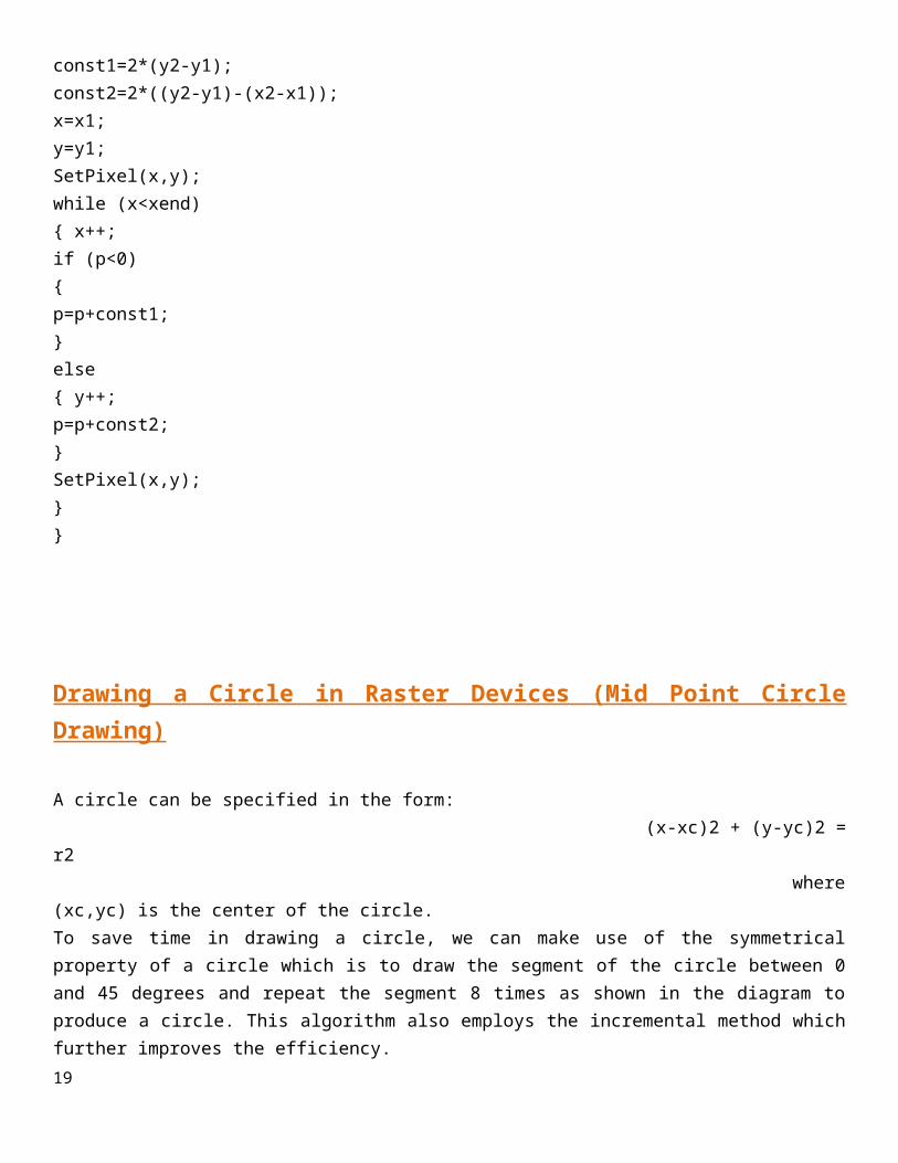
void BresenhamLine(int x1, int y1, int x2, int y2){ int x, y, p, const1, const2; /* initialize variables */p=2*(y2-y1)-(x2-x1);const1=2*(y2-y1);const2=2*((y2-y1)-(x2-x1));x=x1;y=y1;SetPixel(x,y);while (x<xend){ x++;if (p<0){ p=p+const1;}else{ y++;p=p+const2;}SetPixel(x,y);}}

14

Drawing a Circle in Raster Devices (Mid Point Circle Drawing)

A circle can be specified in the form: (x-xc)2 + (y-yc)2 = r2 where (xc,yc) is the center of the circle.

To save time in drawing a circle, we can make use of the symmetrical property of a circle which is to draw the segment of the circle between 0 and 45 degrees and repeat the segment 8 times as shown in the diagram to produce a circle. This algorithm also employs the incremental method which further improves the efficiency.

Algorithm:-

void PlotCirclePoints(int centerx, int centery, int x, int y){ SetPixel(centerx+x,centery+y);SetPixel(centerx-x,centery+y);SetPixel(centerx+x,centery-y);SetPixel(centerx-x,centery-y);SetPixel(centerx+y,centery+x);SetPixel(centerx-y,centery+x);SetPixel(centerx+y,centery-x);SetPixel(centerx-y,centery-x);}void BresenhamCircle(int centerx, int centery, int radius){ int x=0;int y=radius;int p=3-2*radius;while (x<y){ PlotCirclePoints(centerx,centery,x,y);if (p<0)

15

{ p=p+4*x+6;}else{ p=p+4*(x-y)+10;y=y-1;}x=x+1;}PlotCirclePoints(centerx,centery,x,y);}

Ellipses

• Implicit: This is only for the special case where the ellipse is centered at theorigin with the major and minor axes aligned with y = 0 and x = 0.

The implicit form of ellipses and circles is common because there is no explicit functional form.This is because y is a multifunction of x.

16

2D Transformations

Given a point cloud, polygon, or sampled parametric curve, we can use transformations for several purposes:1. Change coordinate frames (world, window, viewport, device, etc).2. Compose objects of simple parts with local scale/position/orientation of one part defined with regard to other parts.

For example, for articulated objects.3. Use deformation to create new shapes.4. Useful for animation.

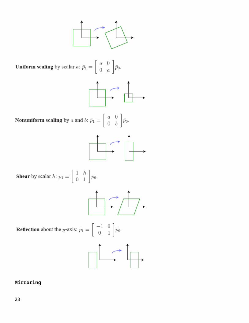
There are three basic classes of transformations:1. Rigid body - Preserves distance and angles.• Examples: translation and rotation.2. Conformal - Preserves angles.• Examples: translation, rotation, and uniform scaling.3. Affine - Preserves parallelism. Lines remain lines.• Examples: translation, rotation, scaling, shear, and reflection.

17

Mirroring

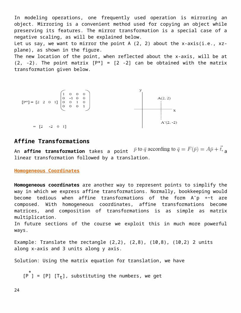
In modeling operations, one frequently used operation is mirroring an object. Mirroring is a convenient method used for copying an object while preserving its features. The mirror transformation is a special case of a negative scaling, as will be explained below. Let us say, we want to mirror the point A (2, 2) about the x-axis(i.e., xz-plane), as shown in the figure. The new location of the point, when reflected about the x-axis, will be at (2, -2). The point matrix [P*] = [2 -2] can be obtained with the matrix transformation given below.

18

Affine TransformationsAn affine transformation takes a point a linear transformation followed by a translation.

Homogeneous Coordinates

Homogeneous coordinates are another way to represent points to simplify the way in which we express affine transformations. Normally, bookkeeping would become tedious when affine transformations of the form A¯p +~t are composed. With homogeneous coordinates, affine transformations become matrices, and composition of transformations is as simple as matrix multiplication.In future sections of the course we exploit this in much more powerful ways.

Example: Translate the rectangle (2,2), (2,8), (10,8), (10,2) 2 units along x-axis and 3 units along y axis.

Solution: Using the matrix equation for translation, we have

[P*] = [P] [Tt], substituting the numbers, we get

19

Module-II

20

Scan-Line Polygon Fill Algorithm

Basic idea: For each scan line crossing a polygon, this algorithm locates the intersection points of the scan line with the polygon edges. These intersection points are shorted from left to right.Then, we fill the pixels between each intersection pair.

Some scan-line intersection at polygon vertices require special handling. A scan line passing through a vertex as intersecting the polygon twice. In this case we may or may not add 2 points to the list of intersections, instead of adding 1 points. This decision depends on whether the 2 edges at both sides of the vertex are both above, both below, or one is above and one is below the scan line. Only for the case if both are above or both are below the scan line, then we will add 2 points.

Inside-Outside Tests: The above algorithm only works for standard polygon shapes. However, for the cases which the edges of the polygon intersect, we need to identify whether a point is an interior or exterior point. Students may find interesting descriptions of 2 methods to solve this problem in many text books: odd-even rule and nonzero winding number rule.

21

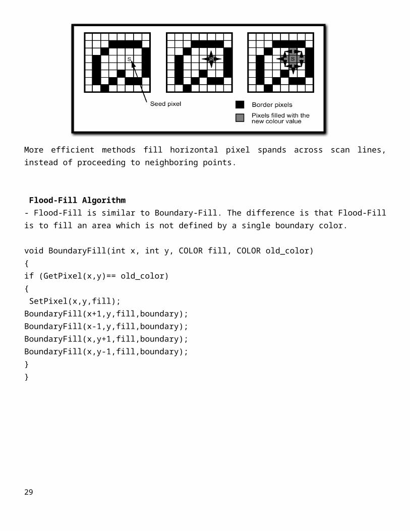
Boundary-Fill Algorithm

- This algorithm starts at a point inside a region and paint the interior outward towards the boundary.- This is a simple method but not efficient: 1. It is recursive method which may occupy a large stack size in the main memory.

void BoundaryFill(int x, int y, COLOR fill, COLOR boundary){ COLOR current;current=GetPixel(x,y);if (current<>boundary) and (current<>fill) then{ SetPixel(x,y,fill);BoundaryFill(x+1, y, fill, boundary);BoundaryFill(x-1, y, fill, boundary);BoundaryFill(x, y+1, fill, boundary);BoundaryFill(x, y-1,fill, boundary);}}

22

More efficient methods fill horizontal pixel spands across scan lines, instead of proceeding to neighboring points.

Flood-Fill Algorithm- Flood-Fill is similar to Boundary-Fill. The difference is that Flood-Fill is to fill an area which is not defined by a single boundary color.

void BoundaryFill(int x, int y, COLOR fill, COLOR old_color){ if (GetPixel(x,y)== old_color){ SetPixel(x,y,fill);BoundaryFill(x+1,y,fill,boundary);BoundaryFill(x-1,y,fill,boundary);BoundaryFill(x,y+1,fill,boundary);BoundaryFill(x,y-1,fill,boundary);}}

23

AntialiasingWhat anti-aliasing attempts to do is, using mathematics, fill in some of the digital system with colors that are in-between the two adjoining colors. In this case a medium gray would be between the black and the white. Some gray squares placed in the grid might help soften up the "jaggies".

Antialiasing utilizes blending techniques to blur the edges of the lines and provide the viewer with the illusion of a smoother line.

Two general approaches: Super-sampling samples at higher resolution, then filters down the resulting image Sometimes called post-filtering The prevalent form of anti-aliasing in hardware Area sampling sample primitives with a box (or Gaussian, or whatever) rather than spikes Requires primitives that have area (lines with width)

Unweighted Area Sampling

• Intensity is proportional to the amount of area covered.

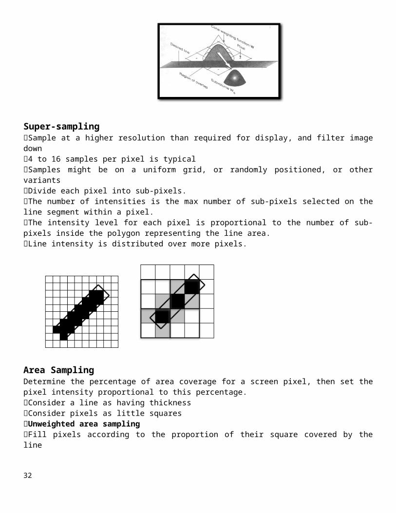
• Defining the box weighting function which has volume of 1 (Imax).

• Determine the overlap volume Ws [0, 1].

• primitive cannot affect intensity of pixel if it does not intersect the pixel • equal areas cause equal intensity, regardless of distance from pixel center to area • Un-weighted sampling colors two pixels identically when the primitive cuts the same area through the

two pixels • intuitively, pixel cut through the center should be more heavily weighted than one cut along corner

24

Weighted Area Sampling

Weight the subpixel contributions according to position, giving higher weights to the central subpixels. Weighting function, W(x,y) specifies the contribution of primitive passing through the point (x, y) from pixel center.

Super-sampling Sample at a higher resolution than required for display, and filter image down 4 to 16 samples per pixel is typical Samples might be on a uniform grid, or randomly positioned, or other variants Divide each pixel into sub-pixels. The number of intensities is the max number of sub-pixels selected on the line segment within a pixel. The intensity level for each pixel is proportional to the number of sub-pixels inside the polygon

representing the line area. Line intensity is distributed over more pixels.

Area Sampling

Determine the percentage of area coverage for a screen pixel, then set the pixel intensity proportional to this percentage.

Consider a line as having thickness Consider pixels as little squares Unweighted area sampling Fill pixels according to the proportion of their square covered by the line

25

Halftone Patterns and Dithering

Halftoning is used when an output device has a limited intensity range, but we want to create an apparent increase in the number of available intensities.Example: The following shows an original picture and the display of it in output devices of limited intensity ranges (4 colors, 8 colors, 16 colors):

If we view a very small area from a sufficiently large viewing distance, our eyes average fine details within the small area and record only the overall intensity of the area. By halftoning, each small resolution unit is imprinted with a circle of black ink whose area is proportional to the blackness of the area in the original photograph. Graphics output devices can approximate the variable-area circles of halftone reproduction by incorporating multiple pixel positions into the display of each intensity value.

A 2 x 2 pixel grid used to display 5 intensity levels (I) on a bilevel system:

26

A 3 x 3 pixel grid used to display 10 intensities on a bilevel system:

A 2x2 pixel grid used to display 13 intensities on a 4-level system:

Dithering

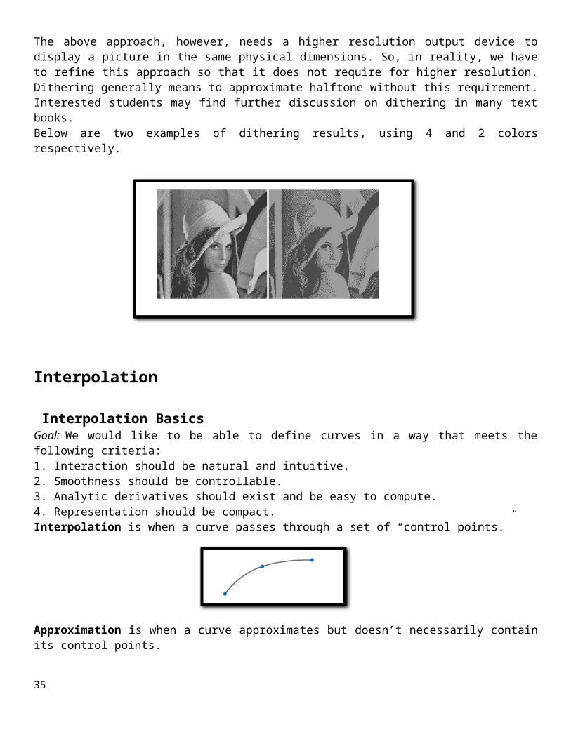
The above approach, however, needs a higher resolution output device to display a picture in the same physical dimensions. So, in reality, we have to refine this approach so that it does not require for higher resolution. Dithering generally means to approximate halftone without this requirement. Interested students may find further discussion on dithering in many text books.Below are two examples of dithering results, using 4 and 2 colors respectively.

27

Interpolation

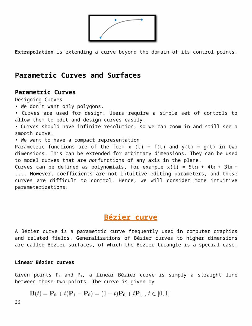
Interpolation BasicsGoal: We would like to be able to define curves in a way that meets the following criteria:1. Interaction should be natural and intuitive.2. Smoothness should be controllable.3. Analytic derivatives should exist and be easy to compute.4. Representation should be compact.Interpolation is when a curve passes through a set of “control points.”

Approximation is when a curve approximates but doesn’t necessarily contain its control points.

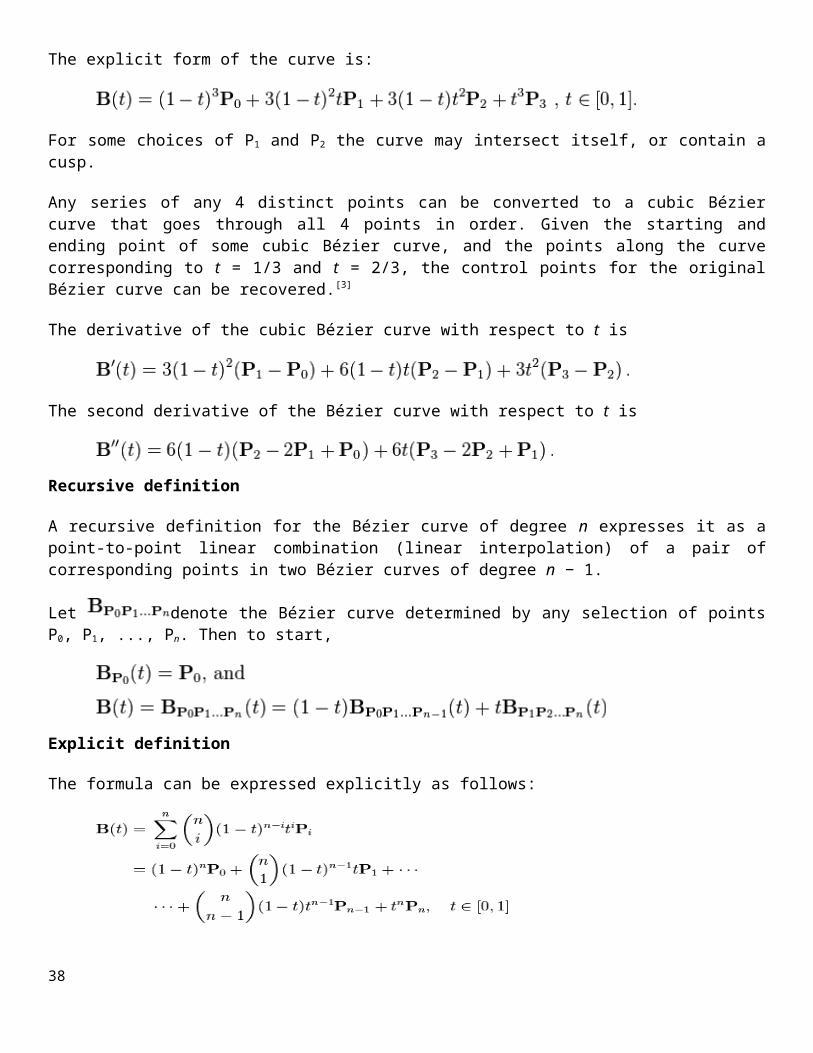
Extrapolation is extending a curve beyond the domain of its control points.

Parametric Curves and Surfaces

Parametric CurvesDesigning Curves• We don’t want only polygons.• Curves are used for design. Users require a simple set of controls to allow them to edit and design curves easily.• Curves should have infinite resolution, so we can zoom in and still see a smooth curve.• We want to have a compact representation.Parametric functions are of the form x (t) = f(t) and y(t) = g(t) in two dimensions. This can be extended for arbitrary dimensions. They can be used to model curves that are not functions of any axis in the plane.Curves can be defined as polynomials, for example x(t) = 5t10 + 4t9 + 3t8 + .... However, coefficients are not intuitive editing parameters, and these curves are difficult to control. Hence, we will consider more intuitive parameterizations.

Bézier curve28

A Bézier curve is a parametric curve frequently used in computer graphics and related fields. Generalizations of Bézier curves to higher dimensions are called Bézier surfaces, of which the Bézier triangle is a special case.

Linear Bézier curves

Given points P0 and P1, a linear Bézier curve is simply a straight line between those two points. The curve is given by

and is equivalent to linear interpolation.

Quadratic Bézier curves

A quadratic Bézier curve is the path traced by the function B(t), given points P0, P1, and P2,

,

which can be interpreted as the linear interpolant of corresponding points on the linear Bézier curves from P0 to P1 and from P1 to P2 respectively. Rearranging the preceding equation yields:

The derivative of the Bézier curve with respect to t is

From which it can be concluded that the tangents to the curve at P0 and P2 intersect at P1. As t increases from 0 to 1, the curve departs from P0 in the direction of P1, then bends to arrive at P2 from the direction of P1.

The second derivative of the Bézier curve with respect to t is

A quadratic Bézier curve is also a parabolic segment. As a parabola is a conic section, some sources refer to quadratic Béziers as "conic arcs".[2]

Cubic Bézier curves

Four points P0, P1, P2 and P3 in the plane or in higher-dimensional space define a cubic Bézier curve. The curve starts at P0 going toward P1 and arrives at P3 coming from the direction of P2. Usually, it will not pass through P1

or P2; these points are only there to provide directional information. The distance between P0 and P1 determines "how long" the curve moves into direction P2 before turning towards P3.

Writing BPi,Pj,Pk(t) for the quadratic Bézier curve defined by points Pi, Pj, and Pk, the cubic Bézier curve can be defined as a linear combination of two quadratic Bézier curves:

29

The explicit form of the curve is:

For some choices of P1 and P2 the curve may intersect itself, or contain a cusp.

Any series of any 4 distinct points can be converted to a cubic Bézier curve that goes through all 4 points in order. Given the starting and ending point of some cubic Bézier curve, and the points along the curve corresponding to t = 1/3 and t = 2/3, the control points for the original Bézier curve can be recovered.[3]

The derivative of the cubic Bézier curve with respect to t is

The second derivative of the Bézier curve with respect to t is

Recursive definition

A recursive definition for the Bézier curve of degree n expresses it as a point-to-point linear combination (linear interpolation) of a pair of corresponding points in two Bézier curves of degree n − 1.

Let denote the Bézier curve determined by any selection of points P0, P1, ..., Pn. Then to start,

Explicit definition

The formula can be expressed explicitly as follows:

Where are the binomial coefficients.

For example, for n = 5:

30

Terminology

Some terminology is associated with these parametric curves. We have

Where the polynomials

are known as Bernstein basis polynomials of degree n.

Note that t0 = 1, (1 − t)0 = 1, and that the binomial coefficient, , also expressed as or is:

The points Pi are called control points for the Bézier curve. The polygon formed by connecting the Bézier points with lines, starting with P0 and finishing with Pn, is called the Bézier polygon (or control polygon). The convex hull of the Bézier polygon contains the Bézier curve.

Properties

The curve begins at P0 and ends at Pn; this is the so-called endpoint interpolation property. The curve is a straight line if and only if all the control points are collinear. The start (end) of the curve is tangent to the first (last) section of the Bézier polygon. A curve can be split at any point into two subcurves, or into arbitrarily many subcurves, each of which is

also a Bézier curve. Some curves that seem simple, such as the circle, cannot be described exactly by a Bézier or piecewise

Bézier curve; though a four-piece cubic Bézier curve can approximate a circle (see Bézier spline), with a maximum radial error of less than one part in a thousand, when each inner control point (or offline

point) is the distance horizontally or vertically from an outer control point on a unit circle. More generally, an n-piece cubic Bézier curve can approximate a circle, when each inner control point is

the distance from an outer control point on a unit circle, where t is 360/n degrees,and n > 2. The curve at a fixed offset from a given Bézier curve, often called an offset curve (lying "parallel" to the

original curve, like the offset between rails in a railroad track), cannot be exactly formed by a Bézier curve (except in some trivial cases). However, there are heuristic methods that usually give an adequate approximation for practical purposes. (For example: [1])

Every quadratic Bézier curve is also a cubic Bézier curve, and more generally, every degree n Bézier curve is also a degree m curve for any m > n. In detail, a degree n curve with control points P0, …, Pn is equivalent (including the parametrization) to the degree n + 1 curve with control points P'0, …, P'n + 1,

where . Bézier curves follow the Variation diminishing property.

31

Constructing Bézier curves

Linear curves

Animation of a linear Bézier curve, t in [0,1]

The t in the function for a linear Bézier curve can be thought of as describing how far B(t) is from P0 to P1. For example when t=0.25, B(t) is one quarter of the way from point P0 to P1. As t varies from 0 to 1, B(t) describes a straight line from P0 to P1.

Quadratic curves

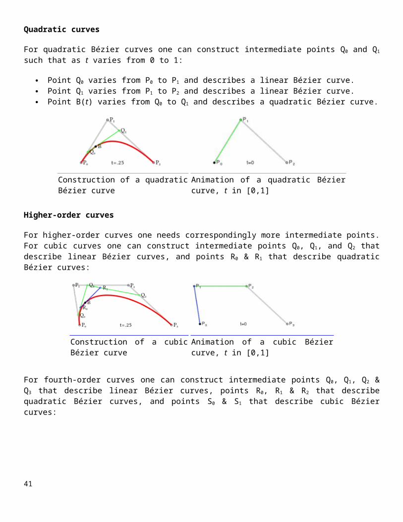
For quadratic Bézier curves one can construct intermediate points Q0 and Q1 such that as t varies from 0 to 1:

Point Q0 varies from P0 to P1 and describes a linear Bézier curve. Point Q1 varies from P1 to P2 and describes a linear Bézier curve. Point B(t) varies from Q0 to Q1 and describes a quadratic Bézier curve.

Construction of a quadratic Bézier curve Animation of a quadratic Bézier curve, t in [0,1]

Higher-order curves

For higher-order curves one needs correspondingly more intermediate points. For cubic curves one can construct intermediate points Q0, Q1, and Q2 that describe linear Bézier curves, and points R0 & R1 that describe quadratic Bézier curves:

Construction of a cubic Bézier curve Animation of a cubic Bézier curve, t in [0,1]

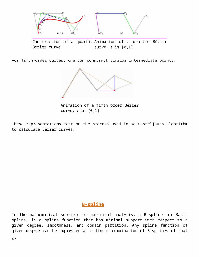
For fourth-order curves one can construct intermediate points Q0, Q1, Q2 & Q3 that describe linear Bézier curves, points R0, R1 & R2 that describe quadratic Bézier curves, and points S0 & S1 that describe cubic Bézier curves:32

Construction of a quartic Bézier curve Animation of a quartic Bézier curve, t in [0,1]

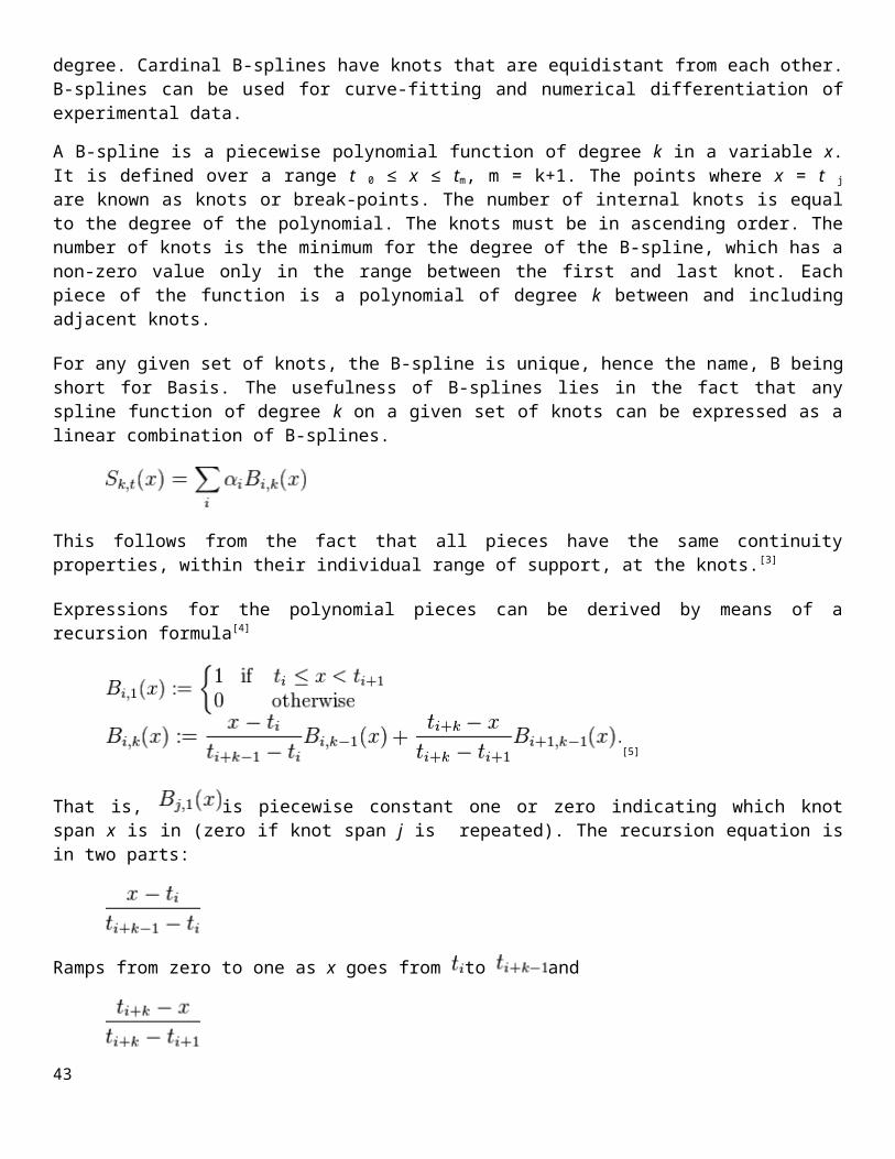
For fifth-order curves, one can construct similar intermediate points.

Animation of a fifth order Bézier curve, t in [0,1]

These representations rest on the process used in De Casteljau's algorithm to calculate Bézier curves.

B-spline

In the mathematical subfield of numerical analysis, a B-spline, or Basis spline, is a spline function that has minimal support with respect to a given degree, smoothness, and domain partition. Any spline function of given degree can be expressed as a linear combination of B-splines of that degree. Cardinal B-splines have knots that are equidistant from each other. B-splines can be used for curve-fitting and numerical differentiation of experimental data.

A B-spline is a piecewise polynomial function of degree k in a variable x. It is defined over a range t 0 ≤ x ≤ tm, m = k+1. The points where x = t j are known as knots or break-points. The number of internal knots is equal to the degree of the polynomial. The knots must be in ascending order. The number of knots is the minimum for the degree of the B-spline, which has a non-zero value only in the range between the first and last knot. Each piece of the function is a polynomial of degree k between and including adjacent knots.

33

For any given set of knots, the B-spline is unique, hence the name, B being short for Basis. The usefulness of B-splines lies in the fact that any spline function of degree k on a given set of knots can be expressed as a linear combination of B-splines.

This follows from the fact that all pieces have the same continuity properties, within their individual range of support, at the knots.[3]

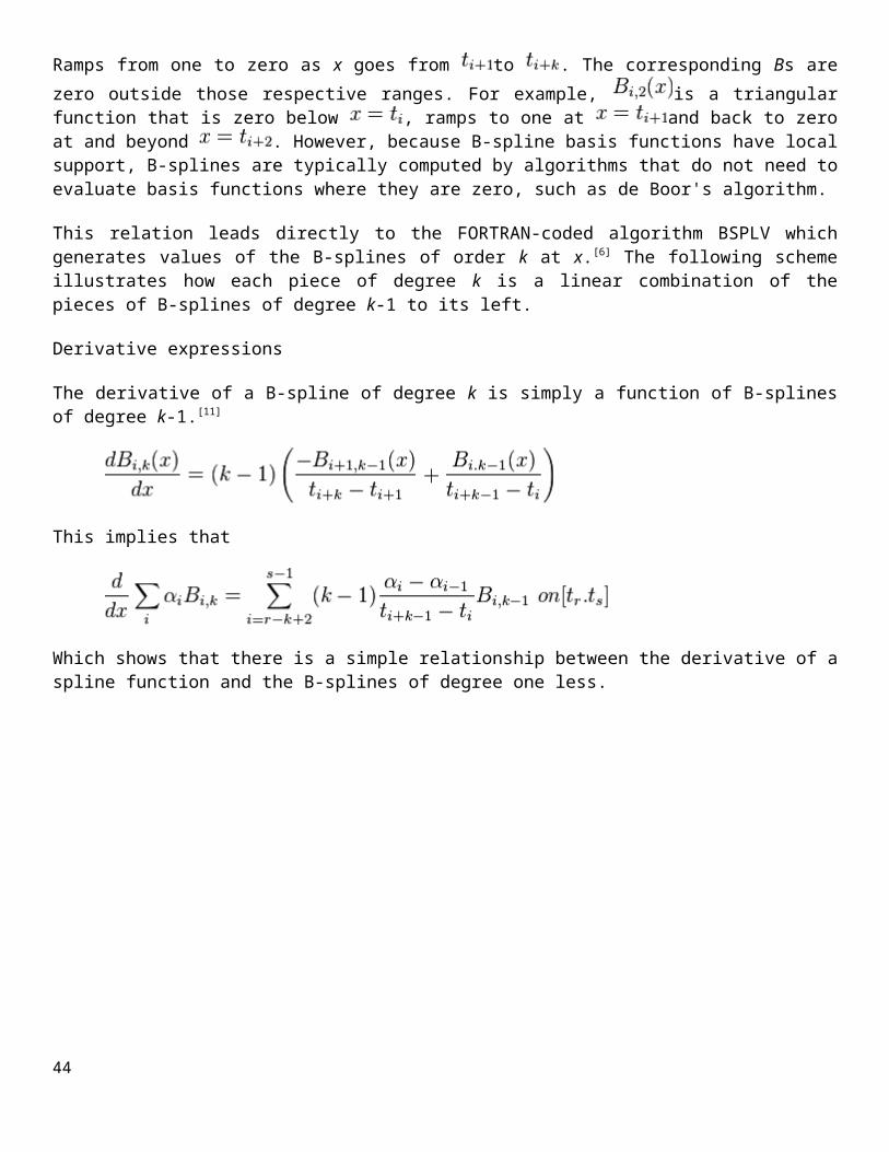
Expressions for the polynomial pieces can be derived by means of a recursion formula[4]

[5]

That is, is piecewise constant one or zero indicating which knot span x is in (zero if knot span j is repeated). The recursion equation is in two parts:

Ramps from zero to one as x goes from to and

Ramps from one to zero as x goes from to . The corresponding Bs are zero outside those respective ranges. For example, is a triangular function that is zero below , ramps to one at and back to zero at and beyond . However, because B-spline basis functions have local support, B-splines are typically computed by algorithms that do not need to evaluate basis functions where they are zero, such as de Boor's algorithm.

This relation leads directly to the FORTRAN-coded algorithm BSPLV which generates values of the B-splines of order k at x.[6] The following scheme illustrates how each piece of degree k is a linear combination of the pieces of B-splines of degree k-1 to its left.

Derivative expressions

The derivative of a B-spline of degree k is simply a function of B-splines of degree k-1.[11]

This implies that34

Which shows that there is a simple relationship between the derivative of a spline function and the B-splines of degree one less.

Fractal Geometry

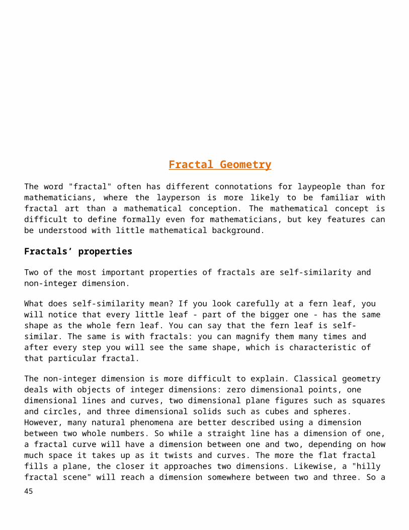
The word "fractal" often has different connotations for laypeople than for mathematicians, where the layperson is more likely to be familiar with fractal art than a mathematical conception. The mathematical concept is difficult to define formally even for mathematicians, but key features can be understood with little mathematical background.

Fractals’ properties

Two of the most important properties of fractals are self-similarity and non-integer dimension.

What does self-similarity mean? If you look carefully at a fern leaf, you will notice that every little leaf - part of the bigger one - has the same shape as the whole fern leaf. You can say that the fern leaf is self-similar. The

35

same is with fractals: you can magnify them many times and after every step you will see the same shape, which is characteristic of that particular fractal.

The non-integer dimension is more difficult to explain. Classical geometry deals with objects of integer dimensions: zero dimensional points, one dimensional lines and curves, two dimensional plane figures such as squares and circles, and three dimensional solids such as cubes and spheres. However, many natural phenomena are better described using a dimension between two whole numbers. So while a straight line has a dimension of one, a fractal curve will have a dimension between one and two, depending on how much space it takes up as it twists and curves. The more the flat fractal fills a plane, the closer it approaches two dimensions. Likewise, a "hilly fractal scene" will reach a dimension somewhere between two and three. So a fractal landscape made up of a large hill covered with tiny mounds would be close to the second dimension, while a rough surface composed of many medium-sized hills would be close to the third dimension.

There are a lot of different types of fractals. In this paper I will present two of the most popular types: complex number fractals and Iterated Function System (IFS) fractals.

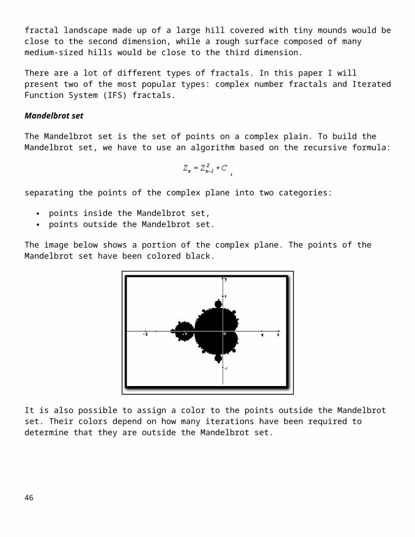
Mandelbrot set

The Mandelbrot set is the set of points on a complex plain. To build the Mandelbrot set, we have to use an algorithm based on the recursive formula:

,

separating the points of the complex plane into two categories:

points inside the Mandelbrot set, points outside the Mandelbrot set.

The image below shows a portion of the complex plane. The points of the Mandelbrot set have been colored black.

It is also possible to assign a color to the points outside the Mandelbrot set. Their colors depend on how many iterations have been required to determine that they are outside the Mandelbrot set.

36

 

 

How is the Mandelbrot set created?

To create the Mandelbrot set we have to pick a point (C ) on the complex plane. The complex number corresponding with this point has the form:

After calculating the value of previous expression:

using zero as the value of , we obtain C as the result. The next step consists of assigning the result to and repeating the calculation: now the result is the complex number . Then we have to assign the value to and repeat the process again and again.

This process can be represented as the "migration" of the initial point C across the plane. What happens to the point when we repeatedly iterate the function? Will it remain near to the origin or will it go away from it, increasing its distance from the origin without limit? In the first case, we say that C belongs to the Mandelbrot set (it is one of the black points in the image); otherwise, we say that it goes to infinity and we assign a color to C depending on the speed at which the point "escapes" from the origin.

We can take a look at the algorithm from a different point of view. Let us imagine that all the points on the plane are attracted by both: infinity and the Mandelbrot set. That makes it easy to understand why:

points far from the Mandelbrot set rapidly move towards infinity, points close to the Mandelbrot set slowly escape to infinity, points inside the Mandelbrot set never escape to infinity.

Julia sets

37

Julia sets are strictly connected with the Mandelbrot set. The iterative function that is used to produce them is the same as for the Mandelbrot set. The only difference is the way this formula is used. In order to draw a picture of the Mandelbrot set, we iterate the formula for each point C of the complex plane, always starting with

. If we want to make a picture of a Julia set, C must be constant during the whole generation process,

while the value of varies. The value of C determines the shape of the Julia set; in other words, each point of the complex plane is associated with a particular Julia set.

How is a Julia set created?

We have to pick a point C) on the complex plane. The following algorithm determines whether or not a point on complex plane Z) belongs to the Julia set associated with C, and determines the color that should be assigned to

it. To see if Z belongs to the set, we have to iterate the function using . What happens to the initial point Z when the formula is iterated? Will it remain near to the origin or will it go away from it, increasing its distance from the origin without limit? In the first case, it belongs to the Julia set; otherwise it goes to infinity and we assign a color to Z depending on the speed the point "escapes" from the origin. To produce an image of the whole Julia set associated with C, we must repeat this process for all the points Z whose coordinates are included in this range:

;

The most important relationship between Julia sets and Mandelbrot set is that while the Mandelbrot set is connected (it is a single piece), a Julia set is connected only if it is associated with a point inside the Mandelbrot

set. For example: the Julia set associated with is connected; the Julia set associated with is not connected (see picture below).

  

Iterated Function System Fractals

Iterated Function System (IFS) fractals are created on the basis of simple plane transformations: scaling, dislocation and the plane axes rotation. Creating an IFS fractal consists of following steps:38

1. defining a set of plane transformations,2. drawing an initial pattern on the plane (any pattern),3. transforming the initial pattern using the transformations defined in first step, 4. transforming the new picture (combination of initial and transformed patterns) using the same set of

transformations,5. repeating the fourth step as many times as possible (in theory, this procedure can be repeated an infinite

number of times).

The most famous ISF fractals are the Sierpinski Triangle and the Koch Snowflake.

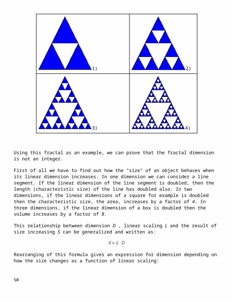
Sierpinski Triangle

This is the fractal we can get by taking the midpoints of each side of an equilateral triangle and connecting them. The iterations should be repeated an infinite number of times. The pictures below present four initial steps of the construction of the Sierpinski Triangle:

1) 2)

3) 4)

 

Using this fractal as an example, we can prove that the fractal dimension is not an integer.

First of all we have to find out how the "size" of an object behaves when its linear dimension increases. In one dimension we can consider a line segment. If the linear dimension of the line segment is doubled, then the length (characteristic size) of the line has doubled also. In two dimensions, if the linear dimensions of a square for example is doubled then the characteristic size, the area, increases by a factor of 4. In three dimensions, if the linear dimension of a box is doubled then the volume increases by a factor of 8.

39

This relationship between dimension D , linear scaling L and the result of size increasing S can be generalized and written as:

Rearranging of this formula gives an expression for dimension depending on how the size changes as a function of linear scaling:

In the examples above the value of D is an integer 1, 2, or 3 depending on the dimension of the geometry. This relationship holds for all Euclidean shapes. How about fractals?Looking at the picture of the first step in building the Sierpinski Triangle, we can notice that if the linear dimension of the basis triangle ( L) is doubled, then the area of whole fractal (blue triangles) increases by a factor of three ( S).

 

Using the pattern given above, we can calculate a dimension for the Sierpinski Triangle:

The result of this calculation proves the non-integer fractal dimension.

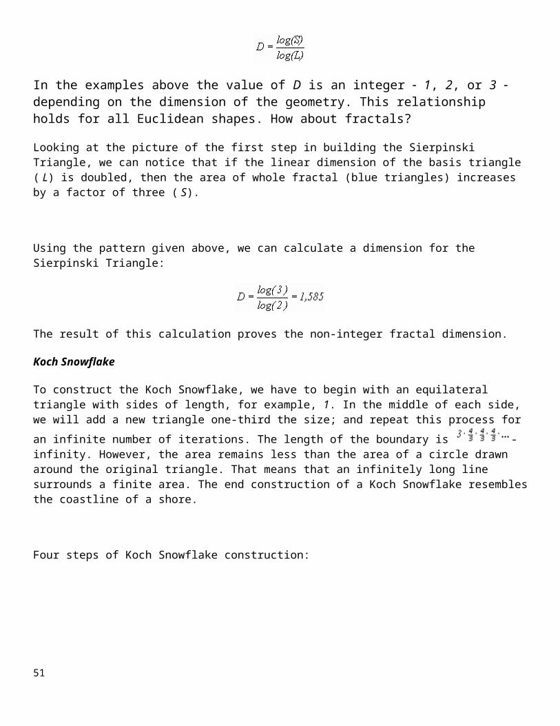
Koch Snowflake

To construct the Koch Snowflake, we have to begin with an equilateral triangle with sides of length, for example, 1. In the middle of each side, we will add a new triangle one-third the size; and repeat this process for

an infinite number of iterations. The length of the boundary is -infinity. However, the area remains less than the area of a circle drawn around the original triangle. That means that an infinitely long line surrounds a finite area. The end construction of a Koch Snowflake resembles the coastline of a shore.

 

Four steps of Koch Snowflake construction:

40

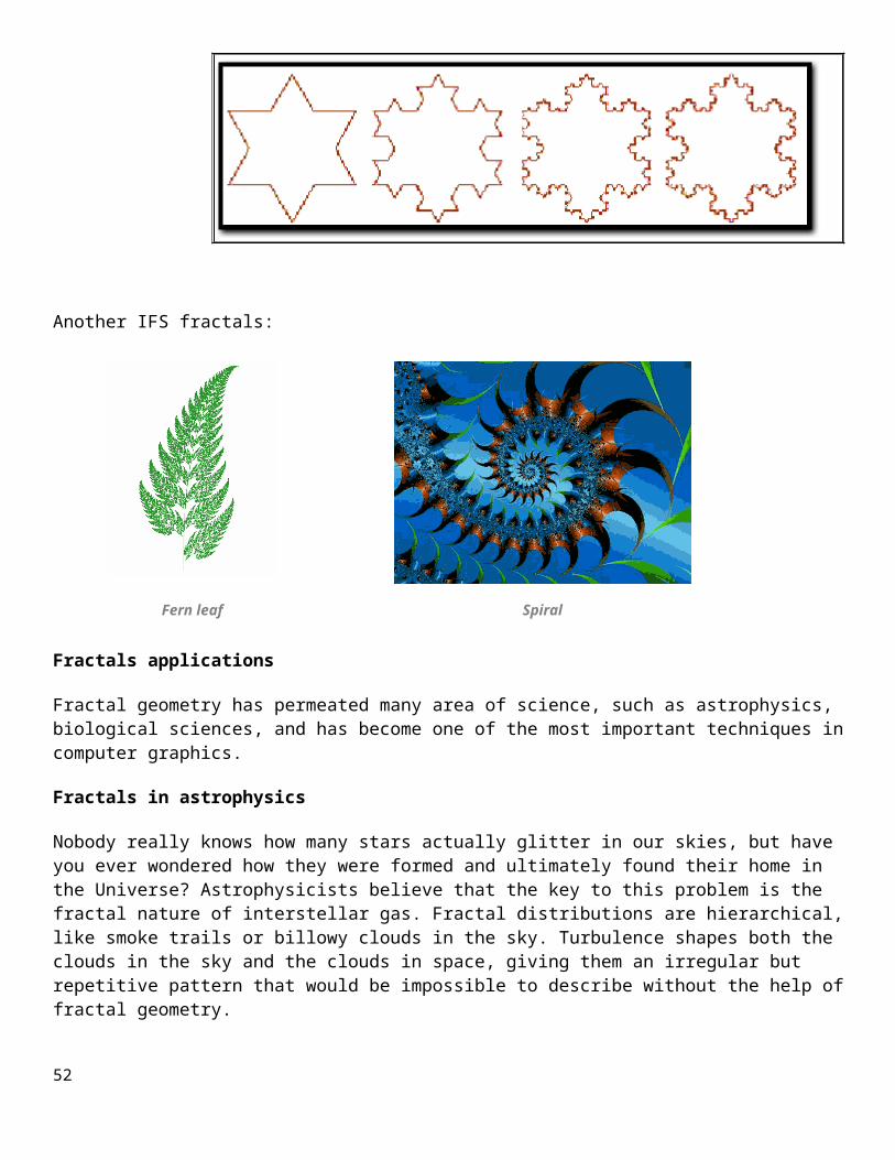
Another IFS fractals:

Fern leaf Spiral

Fractals applications

Fractal geometry has permeated many area of science, such as astrophysics, biological sciences, and has become one of the most important techniques in computer graphics.

Fractals in astrophysics

Nobody really knows how many stars actually glitter in our skies, but have you ever wondered how they were formed and ultimately found their home in the Universe? Astrophysicists believe that the key to this problem is the fractal nature of interstellar gas. Fractal distributions are hierarchical, like smoke trails or billowy clouds in the sky. Turbulence shapes both the clouds in the sky and the clouds in space, giving them an irregular but repetitive pattern that would be impossible to describe without the help of fractal geometry.

Fractals in the Biological Sciences

Biologists have traditionally modeled nature using Euclidean representations of natural objects or series. They represented heartbeats as sine waves, conifer trees as cones, animal habitats as simple areas, and cell membranes as curves or simple surfaces. However, scientists have come to recognize that many natural constructs are better characterized using fractal geometry. Biological systems and processes are typically characterized by many levels of substructure, with the same general pattern repeated in an ever-decreasing cascade. 41

Scientists discovered that the basic architecture of a chromosome is tree-like; every chromosome consists of many 'mini-chromosomes', and therefore can be treated as fractal. For a human chromosome, for example, a fractal dimension D equals 2,34 (between the plane and the space dimension).

Self-similarity has been found also in DNA sequences. In the opinion of some biologists fractal properties of DNA can be used to resolve evolutionary relationships in animals.

Perhaps in the future biologists will use the fractal geometry to create comprehensive models of the patterns and processes observed in nature.

Fractals in computer graphics

The biggest use of fractals in everyday live is in computer science. Many image compression schemes use fractal algorithms to compress computer graphics files to less than a quarter of their original size.

Computer graphic artists use many fractal forms to create textured landscapes and other intricate models.

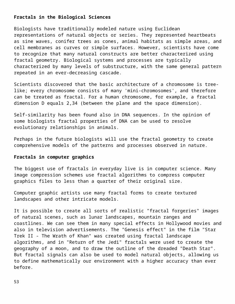
It is possible to create all sorts of realistic "fractal forgeries" images of natural scenes, such as lunar landscapes, mountain ranges and coastlines. We can see them in many special effects in Hollywood movies and also in television advertisements. The "Genesis effect" in the film "Star Trek II - The Wrath of Khan" was created using fractal landscape algorithms, and in "Return of the Jedi" fractals were used to create the geography of a moon, and to draw the outline of the dreaded "Death Star". But fractal signals can also be used to model natural objects, allowing us to define mathematically our environment with a higher accuracy than ever before.

A fractal landscape

 

 

42

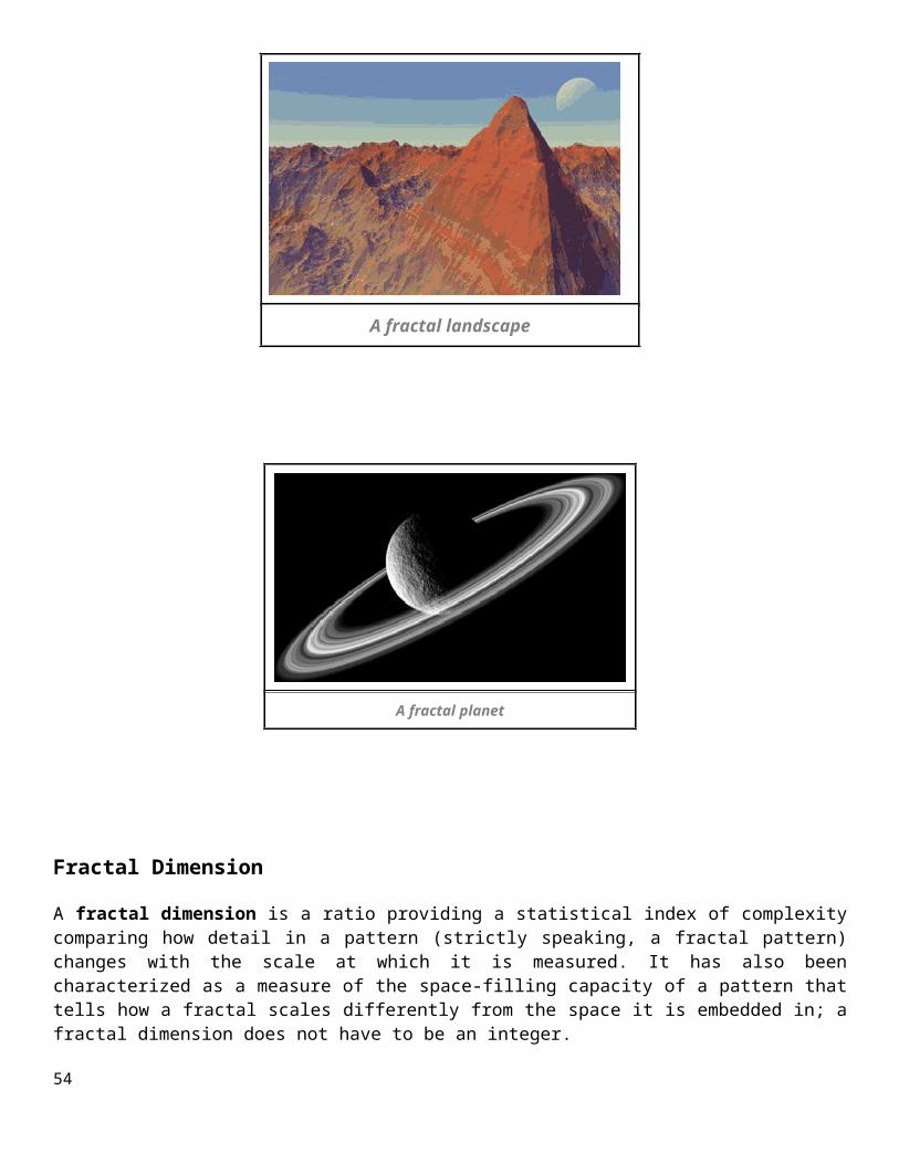
A fractal planet

Fractal Dimension

A fractal dimension is a ratio providing a statistical index of complexity comparing how detail in a pattern (strictly speaking, a fractal pattern) changes with the scale at which it is measured. It has also been characterized as a measure of the space-filling capacity of a pattern that tells how a fractal scales differently from the space it is embedded in; a fractal dimension does not have to be an integer.

Now we see an alternative way to specify the dimension of a self-similar object: The dimension is simply the exponent of the number of self-similar pieces with magnification factor N into which the figure may be broken.

So what is the dimension of the Sierpinski triangle? How do we find the exponent in this case? For this, we need logarithms. Note that, for the square, we have N^2 self-similar pieces, each with magnification factor N. So we can write

Similarly, the dimension of a cube is

43

Thus, we take as the definition of the fractal dimension of a self-similar object

Now we can compute the dimension of S. For the Sierpinski triangle consists of 3 self-similar pieces, each with magnification factor 2. So the fractal dimension is

so the dimension of S is somewhere between 1 and 2, just as our ``eye'' is telling us.

But wait a moment, S also consists of 9 self-similar pieces with magnification factor 4. No problem -- we have

as before. Similarly, S breaks into 3^N self-similar pieces with magnification factors 2^N, so we again have

Fractal dimension is a measure of how "complicated" a self-similar figure is. In a rough sense, it measures "how many points" lie in a given set. A plane is "larger" than a line, while S sits somewhere in between these two sets.

44

Three Dimensional Modeling Transformations

Methods for geometric transforamtions and object modelling in 3D are extended from 2D methods by including the considerations for the z coordinate.Basic geometric transformations are: Translation, Rotation, Scalin

Basic Transformations

Translation

We translate a 3D point by adding translation distances, tx, ty, and tz, to the original coordinate position (x,y,z):x' = x + tx, y' = y + ty, z' = z + tzAlternatively, translation can also be specified by the transformation matrix in the following formula:

Exercise: translate a triangle with vertices at original coordinates (10,25,5), (5,10,5), (20,10,10) bytx=15, ty=5,tz=5. For verification, roughly plot the x and y values of the original and resultant triangles, and imagine the locations of z values.

45

Scaling With Respect to the Origin

We scale a 3D object with respect to the origin by setting the scaling factors sx, sy and sz, which are multiplied to the original vertex coordinate positions (x,y,z):x' = x * sx, y' = y * sy, z' = z * sz

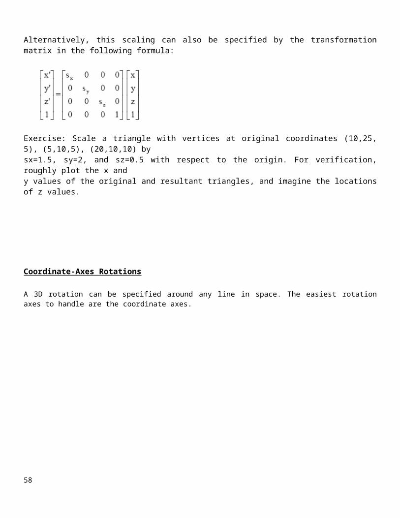
Alternatively, this scaling can also be specified by the transformation matrix in the following formula:

Exercise: Scale a triangle with vertices at original coordinates (10,25, 5), (5,10,5), (20,10,10) bysx=1.5, sy=2, and sz=0.5 with respect to the origin. For verification, roughly plot the x andy values of the original and resultant triangles, and imagine the locations of z values.

Coordinate-Axes Rotations

A 3D rotation can be specified around any line in space. The easiest rotation axes to handle are the coordinate axes.

46

3D Rotations About an Axis Which is Parallel to an Axis

47

Step 1:- Translate the object so that the rotation axis coincides with the parallel coordinate axis.Step 2:-Perform the specified rotation about that axis.Step 3:-Translate the object so that the rotation axis is moved back to its original position.

General 3D Rotations

48

Step 1:-Translate the object so that the rotation axis passes through the coordinate origin.Step 2:- Rotate the object so that the axis of rotation coincides with one of the coordinate axes.Step 3:- Perform the specified rotation about that coordinate axis.Step 4:- Rotate the object so that the rotation axis is brought back to its original orientation.Step 5:- Translate the object so that the rotation axis is brought back to its original position.

Projections

49

Parallel projections

Parallel projections have lines of projection that are parallel both in reality and in the projection plane. Parallel projection corresponds to a perspective projection with an infinite focal length (the distance from the image plane to the projection point), or "zoom". Within parallel projection there is an ancillary category known as "pictorials". Pictorials show an image of an object as viewed from a skew direction in order to reveal all three directions (axes) of space in one picture. Because pictorial projections innately contain this distortion, in the rote, drawing instrument for pictorials, some liberties may be taken for economy of effort and best effect.

Axonometric projection

Axonometric projection is a type of orthographic projection where the plane or axis of the object depicted is not parallel to the projection plane, such that multiple sides of an object are visible in the same image. [5] It is further subdivided into three groups: isometric, dimetric and trimetric projection, depending on the exact angle at which the view deviates from the orthogonal. A typical characteristic of axonometric pictorials is that one axis of space is usually displayed as vertical.

Comparison of several types of graphical projection.

50

Isometric projection

In isometric pictorials (for protocols see isometric projection), the most common form of axonometric projection,[3] the direction of viewing is such that the three axes of space appear equally foreshortened, of which the displayed angles among them and also the scale of foreshortening are universally known. However in creating a final, isometric instrument drawing, in most cases a full-size scale, i.e., without using a foreshortening factor, is employed to good effect because the resultant distortion is difficult to perceive.

Dimetric projection

In dimetric pictorials (for protocols see dimetric projection), the direction of viewing is such that two of the three axes of space appear equally foreshortened, of which the attendant scale and angles of presentation are determined according to the angle of viewing; the scale of the third direction (vertical) is determined separately. Approximations are common in dimetric drawings.

Trimetric projection

In trimetric pictorials (for protocols see trimetric projection), the direction of viewing is such that all of the three axes of space appear unequally foreshortened. The scale along each of the three axes and the angles among them are determined separately as dictated by the angle of viewing. Approximations in trimetric drawings are common,[clarification needed] and trimetric perspective is seldom used.[4]

Oblique projection

In oblique projections the parallel projection rays are not perpendicular to the viewing plane as with orthographic projection, but strike the projection plane at an angle other than ninety degrees.[1] In both orthographic and oblique projection, parallel lines in space appear parallel on the projected image. Because of its simplicity, oblique projection is used exclusively for pictorial purposes rather than for formal, working drawings. In an oblique pictorial drawing, the displayed angles among the axes as well as the foreshortening factors (scale) are arbitrary. The distortion created thereby is usually attenuated by aligning one plane of the imaged object to be parallel with the plane of projection thereby creating a true shape, full-size image of the chosen plane. Special types of oblique projections are cavalier projection and cabinet projection.[2]

Limitations

Objects drawn with parallel projection do not appear larger or smaller as they extend closer to or away from the viewer. While advantageous for architectural drawings, where measurements must be taken directly from the image, the result is a perceived distortion, since unlike perspective projection, this is not how our eyes or photography normally work. It also can easily result in situations where depth and altitude are difficult to gauge, as is shown in the illustration to the right.

In this isometric drawing, the blue sphere is two units higher than the red one. However, this difference in elevation is not apparent if one covers the right half of the picture, as the boxes (which serve as clues suggesting height) are then obscured.

This visual ambiguity has been exploited in op art, including "impossible object" drawings. M. C. Escher's Waterfall (1961) is a well-known example, in which a channel of water seems to travel unaided along a downward path, only to then paradoxically fall once again as it returns to its source. The water thus appears to disobey the law of conservation of energy. An extreme example is depicted in the film Inception, where by a forced perspective trick an immobile stairway changes its connectivity.51

Perspective Projection

Perspective in the graphic arts, such as drawing, is an approximate representation, on a flat surface (such as paper), of an image as it is seen by the eye. The two most characteristic features of perspective are that objects are drawn:

Smaller as their distance from the observer increases. Foreshortened: the size of an object's dimensions along the line of sight are relatively shorter than

dimensions across the line of sight

Perspective drawings have a horizon line, which is often implied. This line, directly opposite the viewer's eye, represents objects infinitely far away. They have shrunk, in the distance, to the infinitesimal thickness of a line. It is analogous to (and named after) the Earth's horizon.

Any perspective representation of a scene that includes parallel lines has one or more vanishing points in a perspective drawing. A one-point perspective drawing means that the drawing has a single vanishing point, usually (though not necessarily) directly opposite the viewer's eye and usually (though not necessarily) on the horizon line. All lines parallel with the viewer's line of sight recede to the horizon towards this vanishing point. This is the standard "receding railroad tracks" phenomenon. A two-point drawing would have lines parallel to two different angles. Any number of vanishing points are possible in a drawing, one for each set of parallel lines that are at an angle relative to the plane of the drawing.

Perspectives consisting of many parallel lines are observed most often when drawing architecture (architecture frequently uses lines parallel to the x, y, and z axes). Because it is rare to have a scene consisting solely of lines parallel to the three Cartesian axes (x, y, and z), it is rare to see perspectives in practice with only one, two, or three vanishing points; even a simple house frequently has a peaked roof which results in a minimum of six sets of parallel lines, in turn corresponding to up to six vanishing points.

In contrast, natural scenes often do not have any sets of parallel lines and thus no vanishing points.

Orthographic projections:

When the observer is at a finite distance from the object, the visual rays or the projectors converge to the eye. But if the observer is imagined at an infinite distance from the transparent plane or the plane projection, the projectors will be parallel and will be perpendicular to the plane of projection as shown in fig (3.1). This projection is called orthographic projection.

52

Module-III

53

Light Intensities

Values of intensity calculated by an illumination model must be converted to one of the allowable intensity levels for the particular graphics system in use.

We have 2 issues to consider:1. Human perceive relative light intensities on a logarithmic scale.

Eg. We perceive the difference between intensities 0.20 and 0.22 to be the same as the difference between 0.80 and 0.88. Therefore, to display successive intensity levels with equal perceived differences of brightness, the intensity levels on the monitor should be spaced so that the ratio of successive intensities is constant:

I1/I0 = I2/I1 = I3/I2 = … = a constant.

2. The intensities produced by display devices are not linear with the electron-gun voltage.This is solved by applying a gamma correction for video lookup correction:Voltage for intensity Ik is computed as:

Vk = (Ik / a )1 / ?Where a is a constant and ? is an adjustment factor controlled by the user.

For example, the NTSC signal standard is ?=2.2.

Basic Lighting and ReflectionUp to this point, we have considered only the geometry of how objects are transformed and projected to images. We now discuss the shading of objects: how the appearance of objects depends, among other things, on the lighting that illuminates the scene, and on the interaction of light with the objects in the scene. Some of the basic qualitative properties of lighting and object reflectance that we need to be able to model include:

Light source - There are different types of sources of light, such as point sources (e.g., a small light at a distance), extended sources (e.g., the sky on a cloudy day), and secondary reflections (e.g., light that bounces from one surface to another).

Reflectance - Different objects reflect light in different ways. For example, diffuse surfaces appear the same when viewed from different directions, whereas a mirror looks very different from different points of view.In this chapter, we will develop simplified model of lighting that is easy to implement and fast to compute, and used in many real-time systems such as OpenGL. This model will be an approximation and does not fully capture all of the effects we observe in the real world. In later chapters, we will discuss more sophisticated and realistic models.

Simple Reflection Models

Diffuse Reflection

We begin with the diffuse reflectance model. A diffuse surface is one that appears similarly bright from all viewing directions. That is, the emitted light appears independent of the viewing location. Let ¯p be a point on a diffuse surface with normal ~n, light by a point light source in direction ~s from the surface. The reflected intensity of light is given by:54

Perfect Specular Reflection

For pure specular (mirror) surfaces, the incident light from each incident direction ~di is reflected toward a unique emittant direction ~de. The emittant direction lies in the same plane as the incident direction ~di and the surface normal ~n, and the angle between ~n and ~de is equal to that between ~n and ~di. One can show that the emitting direction is given by ~de = 2(~n · ~di)~n − ~di. (The derivation was

covered in class). In perfect specular reflection, the light emitted in direction ~de can be computed by reflecting ~de across the normal (as 2(~n · ~de)~n − ~de), and determining the incoming light in this direction. (Again, all vectors are required to be normalized in these equations).

General Specular Reflection

Many materials exhibit a significant specular component in their reflectance. But few are perfect mirrors. First, most specular surfaces do not reflect all light, and that is easily handled by introducing a scalar constant to attenuate intensity. Second, most specular surfaces exhibit some form of off-axis specular reflection. That is, many polished and shiny surfaces (like plastics and metals) emit light in the perfect mirror direction and in some nearby directions as well. These off-axis specularities look a little blurred. Good examples are highlights on plastics and metals. More precisely, the light from a distant point source in the direction of ~s is reflected into a range of directions about the perfect mirror directions ~m = 2(~n · ~s)~n−~s. One common model for this is the following:

Where rs is called the specular reflection coefficient I is the incident power from the point source, and α ≥ 0 is a constant that determines the width of the specular highlights. As α increases, the effective width of the specular reflection decreases. In the limit as α increases, this becomes a mirror.

Ambient Illumination

The diffuse and specular shading models are easy to compute, but often appear artificial. The biggest issue is the point light source assumption, the most obvious consequence of which is that any surface normal pointing away from the light source (i.e., for which ~s · ~n < 0) will have a radiance of zero. A better approximation to the light source is a uniform ambient term plus a point light source. This is a still a remarkably crude model, but it’s much better than the point source by itself. Ambient illumintation is modeled simply by:

55

Where ra is often called the ambient reflection coefficient, and Ia denotes the integral of the uniform illuminant.

Backface Removal

Consider a closed polyhedral object. Because it is closed, far side of the object will always be invisible, blocked by the near side. This observation can be used to accelerate rendering, by removing back-faces.

We can determine if a face is back-facing as follows. Suppose we compute a normals ~n for a mesh face, with the normal chosen so that it points outside the object For a surface point ¯p on a planar patch and eye point ¯e, if (¯p − ¯e) · ~n > 0, then the angle between the view direction and normal is less than 90◦, so the surface normal points away from ¯e. The result will be the same no matter which face point ¯p we use. Patch and eye point ¯e, if (¯p − ¯e) · ~n > 0, then the angle between the view direction and normal is less than 90◦, so the surface normal points away from ¯e. The result will be the same no matter which face point ¯p we use.

Backface removal is a “quick reject” used to accelerate rendering. It must still be used together with another visibility method. The other methods are more expensive, and removing backfaces just reduces the number of faces that must be considered by a more expensive method.

The Depth Buffer

Normally when rendering, we compute an image buffer I(i,j) that stores the color of the object that projects to pixel (i, j). The depth d of a pixel is the distance from the eye point to the object.The depth buffer is an array zbuf(i, j) which stores, for each pixel (i, j), the depth of the nearest point drawn so far. It is initialized by setting all depth buffer values to infinite depth:

zbuf(i,j)= ∞.To draw color c at pixel (i, j) with depth d:if d < zbuf(i, j) thenputpixel(i, j, c)zbuf(i, j) = dend

When drawing a pixel, if the new pixel’s depth is greater than the current value of the depth buffer56

at that pixel, then there must be some object blocking the new pixel, and it is not drawn.

Advantages

• Simple and accurate• Independent of order of polygons drawnDisadvantages

• Memory required for depth buffer• Wasted computation on drawing distant points that are drawn over with closer points that occupy the same pixelTo represent the depth at each pixel, we can use pseudodepth, which is available after the homogeneous perspective transformation.1 Then the depth buffer should be initialized to 1, since the pseudodepth values are between −1 and 1. Pseudo depth gives a number of numerical advantages over true depth.

Painter’s Algorithm

The painter’s algorithm is an alternative to depth buffering to attempt to ensure that the closest points to a viewer occlude points behind them. The idea is to draw the most distant patches of a surface first, allowing nearer surfaces to be drawn over them.In the heedless painter’s algorithm, we first sort faces according to depth of the vertex furthest from the viewer. Then faces are rendered from furthest to nearest. There are problems with this approach, however. In some cases, a face that occludes part of another face can still have its furthest vertex further from the viewer than any vertex of the face it occludes.In this situation, the faces will be rendered out of order. Also, polygons cannot intersect at all as they can when depth buffering is used instead. One solution is to split triangles, but doing this correctly is very complex and slow. Painter’s algorithm is rarely used directly in practice; however, a data-structure called BSP trees can be used to make painter’s algorithm much more appealing.

57

AnimationOverview

Motion can bring the simplest of characters to life. Even simple polygonal shapes can convey a number of human qualities when animated: identity, character, gender, mood, intention, emotion, and so on.The basic principle of animation is the same for all media – displaying a rapid sequence of images which are slightly different than each other creating the illusion of movement before the eye.However, this is how regular, 2D animation is created (or rather, was created until a few years ago). Nowadays, for both creating 2D as well as 3D animation, computer software from several vendors such as Adobe, Xara, Strata and Corel are available.

A movie is a sequence of frames of still images. For video, the frame rate is typically 24 frames per second. For film, this is 30 frames per second.

In general, animation may be achieved by specifying a model with n parameters that identify degrees of freedom that an animator may be interested in such as:-

58

• Polygon vertices,• spline control,• Joint angles,• Muscle contraction,• Camera parameters, or• Color.

With n parameters, this results in a vector ~q in n-dimensional state space. Parameters may be varied to generate animation. A model’s motion is a trajectory through its state space or a set of motion curves for each parameter over time, i.e. ~q(t), where t is the time of the current frame. Every animation technique reduces to specifying the state space trajectory.The basic animation algorithm is then: for t=t1 to tend: render (~q(t)).Modeling and animation are loosely coupled. Modeling describes control values and their actions. Animation describes how to vary the control values. There are a number of animation techniques, including the following:

• User driven animation– Keyframing– Motion capture

• Procedural animation– Physical simulation– Particle systems– Crowd behaviors

• Data-driven animation

Keyframing

Keyframing is an animation technique where motion curves are interpolated through states at times, (~q1, ..., ~qT ), called keyframes, specified by a user.

59

• Pros:– Very expressive– Animator has complete control over all motion parameters

• Cons:– Very labor intensive– Difficult to create convincing physical realism

• Uses:– Potentially everything except complex physical phenomena such as smoke, water, or fire.

Concepts and Storyboarding

Storyboarding is the process of creating a visual representation of the actual screenplay of the animation’s story. It basically consists of a series of illustrations or images presented in a sequence for pre-visualizing an animation. It is usually an intricate and tedious process as it is supposed to visually convey the actual story of the animation.

Modeling

3D modeling is usually done using specialized computer software and involves developing a mathematical model of any surface of a three dimensional object. This is actually done using 2D images of the object using a process called 3D rendering. Models may be created automatically or manually; the latter is usually done by an artist and is similar to sculpting. An example of a computerized 3D model of a human head is shown next. (Source: http://pabs.us/graphictutorials/wp-content)

Layout

To render objects on the media being used, they must first be placed within a scene, a process known as layout. In this process, the physical and spatial interrelations between the objects contained in a scene are first decided. Next, several techniques such as motion capturing and keyframing are used to capture their movement and deformation over time.

Just as in modeling, layout may also involve physical movement of the objects in the scene, similar to sculpting. An example of the use of layout is shown below in a promotional poster for the film ‘Shrek’.

60

Virtual realityVirtual reality (VR), sometimes referred to as immersive multimedia, is a computer-simulated environment that can simulate physical presence in places in the real world or imagined worlds. Virtual reality can recreate sensory experiences, including virtual taste, sight, smell, sound, touch, etc.

Most current virtual reality environments are primarily visual experiences, displayed either on a computer screen or through special stereoscopic displays, but some simulations include additional sensory information, such as sound through speakers or headphones. Some advanced, haptic systems now include tactile information, generally known as force feedback in medical, gaming and military applications. Furthermore, virtual reality covers remote communication environments which provide virtual presence of users with the concepts of telepresence and telexistence or a virtual artifact (VA) either through the use of standard input devices such as a keyboard and mouse, or through multimodal devices such as a wired glove, the Polhemus, and omnidirectional treadmills. The simulated environment can be similar to the real world in order to create a lifelike experience—for example, in simulations for pilot or combat training—or it can differ significantly from reality, such as in VR games. In practice, it is currently very difficult to create a high-fidelity virtual reality experience, because of technical limitations on processing power, image resolution, and communication bandwidth. However, the technology's proponents hope that such limitations will be overcome as processor, imaging, and data communication technologies become more powerful and cost-effective over time.

Virtual reality is often used to describe a wide variety of applications commonly associated with immersive, highly visual, 3D environments. The development of CAD software, graphics hardware acceleration, head-mounted displays, datagloves, and miniaturization have helped popularize the notion. In the book The Metaphysics of Virtual Reality by Michael R. Heim, seven different concepts of virtual reality are identified: simulation, interaction, artificiality, immersion, telepresence, full-body immersion, and network communication. People often identify VR with head mounted displays and data suits.

The possibility exists to have films and television programmes which are watched with a head-mounted display and computer control of the image so that the viewer appears to be inside the scene with the action going all round. The computer presents the view which corresponds to the direction the viewer is facing, through a system of head-tracking. This would give the viewers the feeling that they are actually going to the scene in person instead of looking at pictures on a screen. The term "virtual space" has been suggested as more specific for this technology, which is described in detail in the article Virtual Space - the movies of the future.

The term "artificial reality", coined by Myron Krueger, has been in use since the 1970s; however, the origin of the term "virtual reality" can be traced back to the French playwright, poet, actor, and director Antonin Artaud. In his seminal book The Theatre and Its Double (1938), Artaud described theatre as "la réalité virtuelle", a virtual reality in which, in Erik Davis's words, "characters, objects, and images take on the phantasmagoric force of alchemy's visionary internal dramas". Artaud claimed that the "perpetual allusion to the materials and the principle of the theater found in almost all alchemical books should be understood as the expression of an identity existing between the world in which the characters, images, and in a general way all that constitutes the

61

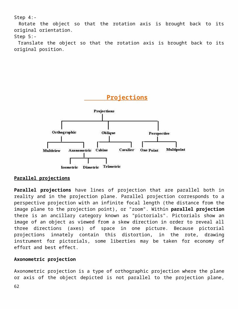
virtual reality of the theater develops, and the purely fictitious and illusory world in which the symbols of alchemy are evolved".

The term has also been used in The Judas Mandala, a 1982 science-fiction novel by Damien Broderick, where the context of use is somewhat different from that defined above. The earliest use cited by the Oxford English Dictionary is in a 1987 article titled "Virtual reality”, but the article is not about VR technology. The concept of virtual reality was popularized in mass media by movies such as Brainstorm and The Lawnmower Man. The VR research boom of the 1990s was accompanied by the non-fiction book Virtual Reality (1991) by Howard Rheingold. The book served to demystify the subject, making it more accessible to less technical researchers and enthusiasts.

Multimedia: from Wagner to Virtual Reality, edited by Randall Packer and Ken Jordan and first published in 2001, explores the term and its history from an avant-garde perspective. Philosophical implications of the concept of VR are discussed in books including Philip Zhai's Get Real: A Philosophical Adventure in Virtual Reality (1998) and Digital Sensations: Space, Identity and Embodiment in Virtual Reality (1999), written by Ken Hillis.

------------------------------------------------------------- X X X X -------------------------------------------------------

62