Lecture Notes in Probability - huji.ac.il · PDF fileLecture Notes in Probability ... to a...
159
Lecture Notes in Probability Raz Kupferman Institute of Mathematics The Hebrew University April 5, 2009
-
Upload
vuongquynh -
Category
Documents
-
view
215 -
download
0
Transcript of Lecture Notes in Probability - huji.ac.il · PDF fileLecture Notes in Probability ... to a...
Lecture Notes in Probability
Raz KupfermanInstitute of MathematicsThe Hebrew University
April 5, 2009

2

Contents
1 Basic Concepts 11.1 The Sample Space . . . . . . . . . . . . . . . . . . . . . . . . . . 11.2 Events . . . . . . . . . . . . . . . . . . . . . . . . . . . . . . . . 31.3 Probability . . . . . . . . . . . . . . . . . . . . . . . . . . . . . . 71.4 Discrete Probability Spaces . . . . . . . . . . . . . . . . . . . . . 101.5 Probability is a Continuous Function . . . . . . . . . . . . . . . . 15
2 Conditional Probability and Independence 212.1 Conditional Probability . . . . . . . . . . . . . . . . . . . . . . . 212.2 Bayes’ Rule and the Law of Total Probability . . . . . . . . . . . 242.3 Compound experiments . . . . . . . . . . . . . . . . . . . . . . . 262.4 Independence . . . . . . . . . . . . . . . . . . . . . . . . . . . . 292.5 Repeated Trials . . . . . . . . . . . . . . . . . . . . . . . . . . . 322.6 On Zero-One Laws . . . . . . . . . . . . . . . . . . . . . . . . . 362.7 Further examples . . . . . . . . . . . . . . . . . . . . . . . . . . 37
3 Random Variables (Discrete Case) 393.1 Basic Definitions . . . . . . . . . . . . . . . . . . . . . . . . . . 393.2 The Distribution Function . . . . . . . . . . . . . . . . . . . . . . 443.3 The binomial distribution . . . . . . . . . . . . . . . . . . . . . . 463.4 The Poisson distribution . . . . . . . . . . . . . . . . . . . . . . 503.5 The Geometric distribution . . . . . . . . . . . . . . . . . . . . . 52

ii CONTENTS
3.6 The negative-binomial distribution . . . . . . . . . . . . . . . . . 533.7 Other examples . . . . . . . . . . . . . . . . . . . . . . . . . . . 533.8 Jointly-distributed random variables . . . . . . . . . . . . . . . . 553.9 Independence of random variables . . . . . . . . . . . . . . . . . 573.10 Sums of random variables . . . . . . . . . . . . . . . . . . . . . . 613.11 Conditional distributions . . . . . . . . . . . . . . . . . . . . . . 63
4 Expectation 674.1 Basic definitions . . . . . . . . . . . . . . . . . . . . . . . . . . . 674.2 The expected value of a function of a random variable . . . . . . . 704.3 Moments . . . . . . . . . . . . . . . . . . . . . . . . . . . . . . 744.4 Using the linearity of the expectation . . . . . . . . . . . . . . . . 784.5 Conditional expectation . . . . . . . . . . . . . . . . . . . . . . . 824.6 The moment generating function . . . . . . . . . . . . . . . . . . 88
5 Random Variables (Continuous Case) 895.1 Basic definitions . . . . . . . . . . . . . . . . . . . . . . . . . . . 895.2 The uniform distribution . . . . . . . . . . . . . . . . . . . . . . 915.3 The normal distribution . . . . . . . . . . . . . . . . . . . . . . . 925.4 The exponential distribution . . . . . . . . . . . . . . . . . . . . 965.5 The Gamma distribution . . . . . . . . . . . . . . . . . . . . . . 985.6 The Beta distribution . . . . . . . . . . . . . . . . . . . . . . . . 985.7 Functions of random variables . . . . . . . . . . . . . . . . . . . 995.8 Multivariate distributions . . . . . . . . . . . . . . . . . . . . . . 1015.9 Conditional distributions and conditional densities . . . . . . . . . 1075.10 Expectation . . . . . . . . . . . . . . . . . . . . . . . . . . . . . 1095.11 The moment generating function . . . . . . . . . . . . . . . . . . 1125.12 Other distributions . . . . . . . . . . . . . . . . . . . . . . . . . 116
6 Inequalities 1196.1 The Markov and Chebyshev inequalities . . . . . . . . . . . . . . 119

CONTENTS iii
6.2 Jensen’s inequality . . . . . . . . . . . . . . . . . . . . . . . . . 121
6.3 Kolmogorov’s inequality . . . . . . . . . . . . . . . . . . . . . . 122
7 Limit theorems 1257.1 Convergence of sequences of random variables . . . . . . . . . . 125
7.2 The weak law of large numbers . . . . . . . . . . . . . . . . . . . 130
7.3 The central limit theorem . . . . . . . . . . . . . . . . . . . . . . 131
7.4 The strong law of large numbers . . . . . . . . . . . . . . . . . . 137
8 Markov chains 1438.1 Definitions and basic properties . . . . . . . . . . . . . . . . . . . 143
8.2 Transience and recurrence . . . . . . . . . . . . . . . . . . . . . 146
8.3 Long-time behavior . . . . . . . . . . . . . . . . . . . . . . . . . 150
9 Simulation 1539.1 Pseudo-random number generators . . . . . . . . . . . . . . . . . 153
9.2 Bernoulli variables . . . . . . . . . . . . . . . . . . . . . . . . . 153
9.3 Exponential variables . . . . . . . . . . . . . . . . . . . . . . . . 154
9.4 Normal variables . . . . . . . . . . . . . . . . . . . . . . . . . . 154
9.5 Rejection sampling . . . . . . . . . . . . . . . . . . . . . . . . . 154
9.6 The Gamma distribution . . . . . . . . . . . . . . . . . . . . . . 156
10 Statistics 15910.1 Notations and some definitions . . . . . . . . . . . . . . . . . . . 159
10.2 Confidence intervals . . . . . . . . . . . . . . . . . . . . . . . . 161
10.3 Su!cient statistics . . . . . . . . . . . . . . . . . . . . . . . . . 164
10.4 Point estimation . . . . . . . . . . . . . . . . . . . . . . . . . . . 167
10.5 Maximum-likelihood estimators . . . . . . . . . . . . . . . . . . 172
10.6 Hypothesis testing . . . . . . . . . . . . . . . . . . . . . . . . . . 176

iv CONTENTS
11 Analysis of variations 18111.1 Introduction . . . . . . . . . . . . . . . . . . . . . . . . . . . . . 181

CONTENTS v
Foreword
These lecture notes were written while teaching the course “Probability 1” at theHebrew University. Most of the material was compiled from a number of text-books, such that A first course in probability by Sheldon Ross, An introduction toprobability theory and its applications by William Feller, and Weighing the oddsby David Williams. These notes are by no means meant to replace a textbook inprobability. By construction, they are limited to the amount of material that canbe taught in a 14 week course of 3 hours. I am grateful to the many students whohave spotted mistakes and helped makes these notes more coherent.

vi CONTENTS

Chapter 1
Basic Concepts
Discussion: Why is probability theory so often a subject of confusion?In every mathematical theory there are three distinct aspects:
! A formal set of rules." An intuitive background, which assigns a meaning to certain concepts.# Applications: when and how can the formal framework be applied to solve
a practical problem.
Confusion may arise when these three aspects intermingle.
Discussion: Intuitive background: what do we mean by “the probability of a diethrow resulting in “5” is 1/6?” Discuss the frequentist versus Bayesian points ofview; explain why the frequentist point of view cannot be used as a fundamentaldefinition of probability (but can certainly guide our intuition).
1.1 The Sample Space
The intuitive meaning of probability is always related to some experiment, whetherreal or conceptual (e.g., winning the lottery, that a newborn be a boy, a person’sheight). We assign probabilities to possible outcomes of the experiment. We firstneed to develop an abstract model for an experiment. In probability theory anexperiment (real or conceptual) is modeled by all its possible outcomes, i.e., by

2 Chapter 1
a set, which we call the sample space. Of course, a set is a mathematical entity,independent of any intuitive background.
Notation: We will usually denote the sample space by " and its elements by !.
Examples:
! Tossing a coin: " = {H,T } (but what if the coin falls on its side or runsaway?).
" Tossing a coin three times:
" = {(a1, a2, a3) : ai ! {H,T }} = {H,T }3.
(Is this the only possibility? for the same experiment we could only observethe majority.)
# Throwing two distinguishable dice: " = {1, . . . , 6}2.$ Throwing two indistinguishable dice: " = {(i, j) : 1 " i " j " 6}.% A person’s lifetime (in years): " = R+ (what about an age limitation?).& Throwing a dart into a unit circle: if we only measure the radius, " = [0, 1].
If we measure position, we could have
" = {(r, ") : 0 " r " 1, 0 " " < 2#} = [0, 1] # [0, 2#),
but also" =!(x, y) : x2 + y2 " 1
".
Does it make a di#erence? What about missing the circle?' An infinite sequence of coin tosses: " = {H,T }$0 (which is isomorphic to
the segment (0, 1)).( Brownian motion: " = C([0, 1];R3).) A person throws a coin: if the result is Head he takes an exam in probability,
which he either passes or fails; if the result is Tail he goes to sleep and wemeasure the duration of his sleep (in hours):
" = {H} #{ 0, 1} %{ T } # R+.
The sample space is the primitive notion of probability theory. It provides a modelof an experiment in the sense that every thinkable outcome (even if extremelyunlikely) is completely described by one, and only one, sample point.

Basic Concepts 3
1.2 Events
Suppose that we throw a die. The set of all possible outcomes (the sample space)is " = {1, . . . , 6}. What about the result ”the outcome is even”? Even outcome isnot an element of ". It is a property shared by several points in the sample space.In other words, it corresponds to a subset of " ({2, 4, 6}). “The outcome is even”is therefore not an elementary outcome of the experiment. It is an aggregate ofelementary outcomes, which we will call an event.
Definition 1.1 An event is a property for which it is clear for every ! ! "whether it has occurred or not. Mathematically, an event is a subset of the samplespace.
The intuitive terms of “outcome” and “event” have been incorporated within anabstract framework of a set and its subsets. As such, we can perform on events set-theoretic operations of union, intersection and complementation. All set-theoreticrelations apply as they are to events.Let " be a sample space which corresponds to a certain experiment. What is thecollection of all possible events? The immediate answer is P("), which is the setof all subsets (denoted also by 2"). It turns out that in many cases it is advisableto restrict the collection of subsets to which probabilistic questions apply. In otherwords, the collection of events is only a subset of 2". While we leave the reasonsto a more advanced course, there are certain requirements that the set of eventshas to fulfill:
! If A & " is an event so is Ac (if we are allowed to ask whether A hasoccurred, we are allowed to ask whether it has not occurred).
" If A, B & " are events, so is A ' B.# " is an event (we can always ask ”has any outcome occurred?”).
A collection of events satisfying these requirements is called an algebra of events.
Definition 1.2 Two events A, B are called disjoint if their intersection is empty.A collection of events is called mutually disjoint if every pair is disjoint. Let A, Bbe events, then
A ' Bc = {! ! " : (! ! A) and (! ! B)} ( A \ B.
Unions of disjoint sets are denoted by %· .

4 Chapter 1
Proposition 1.1 Let " be a sample space and C be an algebra of events. Then,
! ) ! C ." If A1, . . . , An ! C then %n
i=1Ai ! C .# If A1, . . . , An ! C then 'n
i=1Ai ! C .
Proof : Easy. Use de Morgan and induction. *
Probability theory is often concerned with infinite sequences of events. A collec-tion of events C is called a $-algebra of events, if it is an algebra, and in addition,(An)*n=1 + C implies that
*#
n=1
An ! C .
That is, a$-algebra of events is closed with respect to countably many set-theoreticoperations. We will usually denote the $-algebra by F .
Discussion: Historic background on the countably-many issue.
Examples:
! A tautological remark: for every event A,
A = {! ! " : ! ! A} .
" For every ! ! " the singleton {!} is an event.# The experiment is tossing three coins and the event is “second toss was
Head”.$ The experiment is “waiting for the fish to bite” (in hours), and the event is
“waited more than an hour and less than two”.% For every event A, {), A, Ac,"} is a $-algebra of events.& For every collection of events we can construct the $-algebra generated by
this collection.' The cylinder sets in Brownian motion.

Basic Concepts 5
+ Exercise 1.1 Construct a sample space corresponding to filling a single col-umn in the Toto. Define two events that are disjoint. Define three events that aremutually disjoint, and whose union is ".
Infinite sequences of events Let (",F ) be a sample space together with a $-algebra of events (such a pair is called a measurable space), and let (An)*n=1 + F .We have *$
n=1
An = {! ! " : ! ! An for at least one n}
*#
n=1
An = {! ! " : ! ! An for all n} .
Also,*$
k=n
Ak = {! ! " : ! ! Ak for at least one k , n}
(there exists a k , n for which ! ! Ak), so that
*#
n=1
*$
k=n
Ak =%! ! " : ! ! Ak for infinitely many k
&
(for every n there exists a k , n for which ! ! Ak). We denote,
*#
n=1
*$
k=n
Ak = {! ! " : ! ! Ak i.o.} ( lim supn
An.
Similarly,*#
k=n
Ak = {! ! " : ! ! Ak for all k , n}
(! ! Ak for all k , n), so that
*$
n=1
*#
k=n
Ak =%! ! " : ! ! Ak eventually
& ( lim infn
An
(there exists an n such that ! ! Ak for all k , n). Clearly,
lim infn
An & lim supn
An.
6 Chapter 1
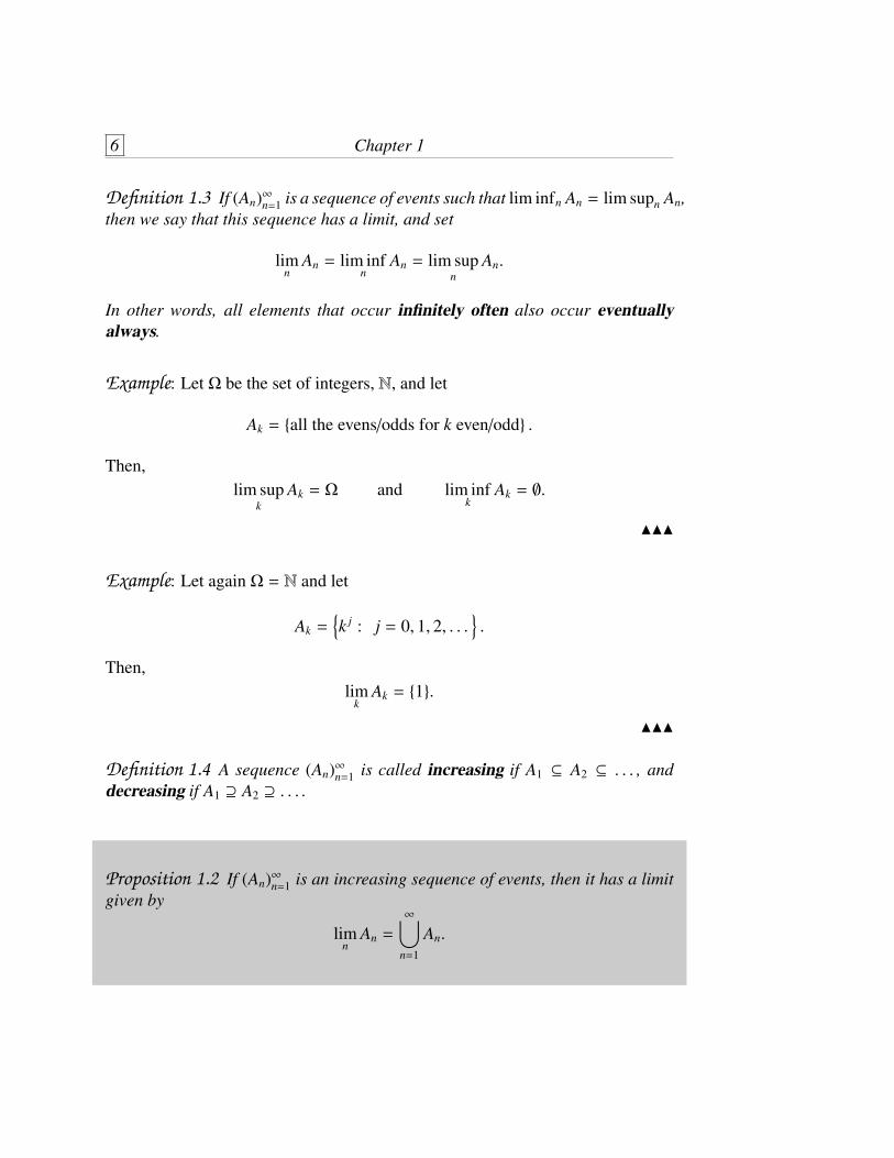
Definition 1.3 If (An)*n=1 is a sequence of events such that lim infn An = lim supn An,then we say that this sequence has a limit, and set
limn
An = lim infn
An = lim supn
An.
In other words, all elements that occur infinitely often also occur eventuallyalways.
Example: Let " be the set of integers, N, and let
Ak = {all the evens/odds for k even/odd} .
Then,lim sup
kAk = " and lim inf
kAk = ).
!!!
Example: Let again " = N and let
Ak =!k j : j = 0, 1, 2, . . .
".
Then,lim
kAk = {1}.
!!!
Definition 1.4 A sequence (An)*n=1 is called increasing if A1 & A2 & . . . , anddecreasing if A1 - A2 - . . . .
Proposition 1.2 If (An)*n=1 is an increasing sequence of events, then it has a limitgiven by
limn
An =
*$
n=1
An.
Basic Concepts 7
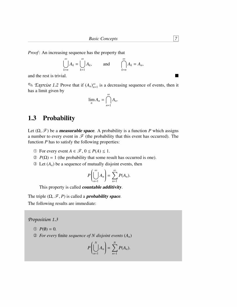
Proof : An increasing sequence has the property that*$
k=n
Ak =
*$
k=1
Ak, and*#
k=n
Ak = An,
and the rest is trivial. *
+ Exercise 1.2 Prove that if (An)*n=1 is a decreasing sequence of events, then ithas a limit given by
limn
An =
*#
n=1
An.
1.3 Probability
Let (",F ) be a measurable space. A probability is a function P which assignsa number to every event in F (the probability that this event has occurred). Thefunction P has to satisfy the following properties:
! For every event A ! F , 0 " P(A) " 1." P(") = 1 (the probability that some result has occurred is one).# Let (An) be a sequence of mutually disjoint events, then
P
'((((()*$
n=1
An
*+++++, =
*-
n=1
P(An).
This property is called countable additivity.
The triple (",F , P) is called a probability space.The following results are immediate:
Proposition 1.3
! P()) = 0." For every finite sequence of N disjoint events (An)
P
'((((()
N$
n=1
An
*+++++, =
N-
n=1
P(An).
8 Chapter 1
Proof : The first claim is proved by noting that for every A ! F , A = A %· ). Forthe second claim we take Ak = ) for k > n. *
Examples:
! Tossing a coin, and choosing P({H}) = P({T }) = 1/2." Throwing a die, and choosing P({i}) = 1/6 for i ! {1, . . . , 6}. Explain why
this defines uniquely a probability function.
Proposition 1.4 For every event A ! F ,
P(Ac) = 1 . P(A).
If A, B are events such that A & B, then
P(A) " P(B).
Proof : The first result follows from the fact that A %· Ac = ". The second resultfollows from B = A %· (B \ A). *
Proposition 1.5 (Probability of a union) Let (",F , P) be a probability space.For every two events A, B ! F ,
P(A % B) = P(A) + P(B) . P(A ' B).
Proof : We haveA % B = (A \ B) %· (B \ A) %· (A ' B)
A = (A \ B) %· (A ' B)B = (B \ A) %· (A ' B),
and it remains to use the additivity of the probability function to calculate P(A %B) . P(A) . P(B). *

Basic Concepts 9
Proposition 1.6 Let (",F , P) be a probability space. For every three eventsA, B,C ! F ,
P(A % B %C) = P(A) + P(B) + P(C). P(A ' B) . P(A 'C) . P(B 'C)+ P(A ' B 'C).
Proof : Using the binary relation we have
P(A % B %C) = P(A % B) + P(C) . P((A % B) 'C)= P(A) + P(B) . P(A ' B) + P(C) . P((A 'C) % (B 'C)),
and it remains to apply the binary relation for the last expression. *
Proposition 1.7 (Inclusion-exclusion principle) For n events (Ai)ni=1 we have
P(A1 % · · · % An) =n-
i=1
P(Ai) .-
i< j
P(Ai ' Aj) +-
i< j<k
P(Ai ' Aj ' Ak)
+ (.1)n+1P(A1 ' · · · ' An)
+ Exercise 1.3 Prove the inclusion-exclusion principle.
+ Exercise 1.4 Let A, B be two events in a probability space. Show that theprobability that either A or B has occurred, but not both, is P(A)+P(B).2 P(A'B).
Lemma 1.1 (Boole’s inequality) Let (",F , P) be a probability space. Probabil-ity is sub-additive in the sense that
P.%*k=1Ak
/ "*-
k=1
P(Ak)
for every sequence (An) of events.
10 Chapter 1
Proof : Define the following sequence of events,
B1 = A1 B2 = A2 \ A1, , . . . , Bn = An \0%n.1
k=1Ak
1.
The Bn are disjoint and their union equals to the union of the An. Also, Bn & An
for every n. Now,
P.%*k=1Ak
/= P.%*k=1Bk
/=
*-
k=1
P(Bk) "*-
k=1
P(Ak).
*
1.4 Discrete Probability Spaces
The simplest sample spaces to work with are such whose sample spaces includecountably many points. Let " be a countable set,
" = {a1, a2, . . . } ,and let F = P("). Then, a probability function, P, on F is fully determinedby its value for every singleton, {aj}, i.e., by the probability assigned to everyelementary event. Indeed, let P({aj}) ( pj be given, then since every event A canbe expressed as a finite, or countable union of disjoint singletons,
A = %· a j!A{aj},it follows from the additivity property that
P(A) =-
a j!Ap j.
A particular case which often arises in applications is when the sample space isfinite (we denote by |"| the size of the sample space), and where every elementaryevent {!} has equal probability, p. By the properties of the probability function,
1 = P(") =-
a j!"P({aj}) = p|"|,
i.e., p = 1/|"|. The probability of every event A is then
P(A) =-
a j!AP({aj}) = p|A| = |A||"| .

Basic Concepts 11
Comment: The probability space, i.e., the sample space, the set of events and theprobability function, are a model of an experiment whose outcome is a priori un-known. There is no a priori reason why all outcomes should be equally probable.It is an assumption that has to be made only when believed to be applicable.
Examples:
! Two dice are rolled. What is the probability that the sum is 7? The samplespace is" = {(i, j) : 1 " i, j " 6}, and it is natural to assume that each of the|"| = 36 outcomes is equally likely. The event ”the sum is 7” correspondsto
A = {(1, 6), (2, 5), (3, 4), (4, 3), (5, 2), (6, 1)} ,so that P(A) = 6/36.
" There are 11 balls in a jar, 6 white and 5 black. Two balls are taken atrandom. What is the probability of having one white and one black.To solve this problem, it is helpful to imagine that the balls are numberedfrom 1 to 11. The sample space consists of all possible pairs,
" = {(i, j) : 1 " i < j " 11} ,and its size is |"| =
0112
1; we assume that all pairs are equally likely. The
event A = one black and one white corresponds to a number of states equalto the number of possibility to choose one white ball out of six, and oneblack ball out of five, i.e.,
P(A) =
061
1051
1
0112
1 =6 · 5
10 · 11 : 2=
611.
# A deck of 52 cards is distributed between four players. What is the proba-bility that one of the players received all 13 spades?The sample space " is the set of all possible partitions, the number of dif-ferent partitions being
|"| = 52!13! 13! 13! 13!
(the number of possibilities to order 52 cards divided by the number ofinternal orders). Let Ai be the event that the i-th player has all spades, andA be the event that some player has all spades; clearly,
A = A1 %· A2 %· A3 %· A4.
12 Chapter 1
For each i,|Ai| =
39!13! 13! 13!
,
hence,
P(A) = 4 P(A1) = 4 # 39! 13! 13! 13! 13!52! 13! 13! 13!
/ 6.3 # 10.12.
+ Exercise 1.5 Prove that it is not possible to construct a probability functionon the sample space of integers, such that P({i}) = P({ j}) for all i, j.
+ Exercise 1.6 A fair coin is tossed five times. What is the probability that therewas at least one instance of two Heads in a row? Start by building the probabilityspace.
We are now going to cover a number of examples, all concerning finite probabilityspaces with equally likely outcomes. The importance of these examples stemsfrom the fact that they are representatives of classes of problems which recur inmany applications.
Example: (The birthday paradox) In a random assembly of n people, what isthe probability that none of them share the same date of birth?We assume that n < 365 and ignore leap years. The sample space is the set ofall possible date-of-birth assignments to n people. This is a sample space of size|"| = 365n. Let An be the event that all dates-of-birth are di#erent. Then,
|An| = 365 # 364 # · · · # (365 . n + 1),
henceP(An) =
|An||"| = 1 # 364
365# · · · # 365 . n + 1
365.
The results for various n are
P(A23) < 0.5 P(A50) < 0.03 P(A100) < 3.3 # 10.7.
!!!
Comment: Many would have guessed that P(A50) / 1.50/365. This is a “selfish”thought.

Basic Concepts 13
Example: (The inattentive secretary, or the matching problem) A secretaryplaces randomly n letters into n envelopes. What is the probability that no letterreaches its destination? What is the probability that exactly k letters reach theirdestination?As usual, we start by setting the sample space. Assume that the letters and en-velopes are all numbered from one to n. The sample space consists of all possibleassignments of letters to envelopes, i.e., the set of all permutations of the numbers1-to-n. The first question can be reformulated as follows: take a random one-to-one function from {1, . . . , n} to itself; what is the probability that it has no fixedpoints?If A is the event that no letter has reached its destination, then its complement, Ac
is the event that at least one letter has reached its destination (at least one fixedpoint). Let furthermore Bi be the event that the i-th letter reached its destination,then
Ac = %ni=1Bi.
We apply the inclusion-exclusion principle:
P(Ac) =n-
i=1
P(Bi) .-
i< j
P(Bi ' Bj) +-
i< j<k
P(Bi ' Bj ' Bk) . . . .
= n P(B1) .2n2
3P(B1 ' B2) +
2n3
3P(B1 ' B2 ' B3) . . . . ,
where we have used the symmetry of the problem. Now,
P(B1) =|B1||"| =
(n . 1)!n!
P(B1 ' B2) =|B1 ' B2||"| =
(n . 2)!n!
,
etc. It follows that
P(Ac) = n1n.2n2
3(n . 2)!
n!+
2n3
3(n . 3)!
n!. · · · + (.1)n+1
2nn
30!n!
= 1 . 12!+
13!. · · · + (.1)n+1 1
n!
=
n-
k=1
(.1)k+1
k!.

14 Chapter 1
For large n,
P(A) = 1 . P(Ac) =n-
k=0
(.1)k
k!/ e.1,
from which we deduce that for large n, the probability that no letter has reachedits destination is 0.37. The fact that the limit is finite may sound surprising (onecould have argued equally well that the limit should be either 0 or 1). Note that asa side result, the number of permutations that have no fixed points is
|A| = |"| P(A) = n!n-
k=0
(.1)k
k!.
Now to the second part of this question. Before we answer what is the numberof permutations that have exactly k fixed points, let’s compute the number of per-mutations that have only k specific fixed points. This number coincides with thenumber of permutations of n . k elements without fixed points,
(n . k)!n.k-
%=0
(.1)%
%!.
The choice of k fixed points is exclusive, so to find the total number of permu-tations that have exactly k fixed points, we need to multiply this number by thenumber of ways to choose k elements out of n. Thus, if C denotes the event thatthere are exactly k fixed points, then
|C| =2nk
3(n . k)!
n.k-
%=0
(.1)%
%!,
and
P(C) =1k!
n.k-
%=0
(.1)%
%!.
For large n and fixed k we have
P(C) / e.1
k!.
We will return to such expressions later on, in the context of the Poisson distri-bution. !!!

Basic Concepts 15
+ Exercise 1.7 Seventeen men attend a party (there were also women, but it isirrelevant). At the end of it, these drunk men collect at random a hat from the hathanger. What is the probability that
! At least someone got his own hat." John Doe got his own hat.# Exactly 3 men got their own hats.$ Exactly 3 men got their own hats, one of which is John Doe.
As usual, start by specifying what is your sample space.
+ Exercise 1.8 A deck of cards is dealt out. What is the probability that thefourteenth card dealt is an ace? What is the probability that the first ace occurs onthe fourteenth card?
1.5 Probability is a Continuous Function
This section could be omitted in a first course on probability. I decided to include it onlyin order to give some flavor of the analytical aspects of probability theory.
An important property of the probability function is its continuity, in the sensethat if a sequence of events (An) has a limit, then P(lim An) = lim P(An).We start with a “soft” version:
Theorem 1.1 (Continuity for increasing sequences) Let (An) be an increasing se-quence of events, then
P(limn
An) = limn
P(An).
Comment: We have already shown that the limit of an increasing sequence ofevents exists,
limn
An = %*k=1Ak.
Note that for every n,P(%n
k=1Ak) = P(An),

16 Chapter 1
but we can’t just replace n by*. Moreover, since P(An) is an increasing functionwe have
P(An)0 P(limn
An).
Proof : Recall that for an increasing sequence of events, limn An = %*n=1An. Con-struct now the following sequence of disjoint events,
B1 = A1
B2 = A2 \ A1
B3 = A3 \ A2,
etc. Clearly,
%· ni=1Bi = %n
i=1Ai = An and hence %*i=1 Ai = %· *i=1Bi.
Now,
P(limn
An) = P(%*i=1Ai) = P(%· *i=1Bi)
=
*-
i=1
P(Bi) = limn
n-
i=1
P(Bi)
= limn
P(%· ni=1Bi) = lim
nP(An).
*
+ Exercise 1.9 (Continuity for decreasing sequences) Prove that if (An) is a de-creasing sequence of events, then
P(limn
An) = limn
P(An),
and more precisely, P(An)1 P(limn An).
Now the next two lemmas are for arbitrary sequences of events, without assumingthe existence of a limit.
Lemma 1.2 (Fatou) Let (An) be a sequence of events, then
P(lim infn
An) " lim infn
P(An).

Basic Concepts 17
Proof : Recall that
lim infn
An = %*n=1 '*k=n Ak ( %*n=1Gn
is the set of outcomes that occur “eventually always”. The sequence (Gn) is in-creasing, and therefore
limn
P(Gn) = P(limn
Gn) = P(lim infn
An).
On the other hand, since Gn = '*k=nAk, it follows that
P(Gn) " infk,n
P(Ak).
The left hand side converges to P(lim infn An) whereas the right hand side con-verges to lim infn P(An), which concludes the proof. *
Lemma 1.3 (Reverse Fatou) Let (An) be a sequence of events, then
lim supn
P(An) " P(lim supn
An).
Proof : Recall that
lim supn
An = '*n=1 %*k=n Ak ( '*n=1Gn
is the set of outcomes that occur “infinitely often”. The sequence (Gn) is decreas-ing, and therefore
limn
P(Gn) = P(limn
Gn) = P(lim supn
An).
On the other hand, since Gn = %*k=nAk, it follows that
P(Gn) , supk,n
P(Ak).
The left hand side converges to P(lim supn An) whereas the right hand side con-verges to lim supn P(An), which concludes the proof. *

18 Chapter 1
Theorem 1.2 (Continuity of probability) If a sequence of events (An) has a limit,then
P(limn
An) = limn
P(An).
Proof : This is an immediate consequence of the two Fatou lemmas, for
lim supn
P(An) " P(lim supn
An) = P(lim infn
An) " lim infn
P(An).
*
Lemma 1.4 (First Borel-Cantelli) Let (An) be a sequence of events such that4n P(An) < *. Then,
P(lim supn
An) = P({An i.o.}) = 0.
Proof : Let as before Gn = %*k=nAk. Since P(Gn)1 P(lim supn An), then for all m
P(lim supn
An) " P(Gm) "-
k,m
P(Ak).
Letting m2 * and using the fact that the right hand side is the tail of a convergingseries we get the desired result. *
+ Exercise 1.10 Does the “reverse Borel-Cantelli” hold? Namely, is it true thatif4
n P(An) = * thenP(lim sup
nAn) > 0.
Well, no. Construct a counter example.
Example: Consider the following scenario. At a minute to noon we insert into anurn balls numbered 1-to-10 and remove the ball numbered “10”. At half a minuteto noon we insert balls numbered 11-to-20 and remove the ball numbered “20”,

Basic Concepts 19
and so on. Which balls are inside the urn at noon? Clearly all integers except forthe “10n”.Now we vary the situation, except that the first time we remove the ball numbered“1”, next time the ball numbered “2”, etc. Which balls are inside the urn at noon?none.In the third variation we remove each time a ball at random (from those insidethe urn). Are there any balls left at noon? If this question is too bizarre, hereis a more sensible picture. Our sample space consists of random sequences ofnumbers, whose elements are distinct, and whose first element is in the range 1-to-10, its second element is in the range 1-to-20, and so on. We are asking what isthe probability that such a sequence contains all integers?Let’s focus on ball number “1” and denote by En then event that it is still insidethe urn after n steps. We have
P(En) =9
10# 18
19# · · · # 9n
9n + 1=
n5
k=1
9k9k + 1
.
The events (En) form a decreasing sequence, whose countable intersection corre-sponds to the event that the first ball was not ever removed. Now,
P(limn
En) = limn
P(En) = limn
n5
k=1
9k9k + 1
= limn
6777778
n5
k=1
9k + 19k
9:::::;.1
= limn
6777778
n5
k=1
21 +
19k
39:::::;.1
= limn
<21 +
19
3 21 +
118
3. . .
=.1
" limn
21 +
19+
118+ . . .
3.1
= 0.
Thus, there is zero probability that the ball numbered “1” is inside the urn afterinfinitely many steps. The same holds ball number “2”, “3”, etc. If Fn denotes theevent that the n-th ball has remained inside the box at noon, then
P(%*n=1Fn) "*-
n=1
P(Fn) = 0.
!!!

20 Chapter 1

Chapter 2
Conditional Probability andIndependence
2.1 Conditional Probability
Example: Two dice are tossed. What is the probability that the sum is 8? This isan easy exercise: we have a sample space " that comprises 36 equally-probableoutcomes. The event “the sum is 8” is given by
A = {(2, 6), (3, 5), (4, 4), (5, 3), (6, 2)} ,
and therefore P(A) = |A|/|"| = 5/36.But now, suppose someone reveals that the first die resulted in “3”. How does thischange our predictions? This piece of information tells us that “with certainty”the outcome of the experiment lies in set
F = {(3, i) : 1 " i " 6} + ".
As this point, outcomes that are not in F have to be ruled out. The sample spacecan be restricted to F (F becomes the certain event). The event A (sum was“8”) has to be restricted to its intersection with F. It seems reasonable that “theprobability of A knowing that F has occurred” be defined as
|A ' F||F| =
|A ' F|/|"||F|/|"| =
P(A ' F)P(F)
,
which in the present case is 1/6. !!!

22 Chapter 2
This example motivates the following definition:
Definition 2.1 Let (",F , P) be a probability space and let F ! F be an eventfor which P(F) " 0. For every A ! F the conditional probability of A giventhat F has occurred (or simply, given F) is defined (and denoted) by
P(A|F) :=P(A ' F)
P(F).
Comment: Note that conditional probability is defined only if the conditioningevent has finite probability.
Discussion: Like probability itself, conditional probability also has di#erent in-terpretations depending on wether you are a frequentist or Bayesian. In the fre-quentist interpretation, we have in mind a large set of n repeated experiments. LetnB denote the number of times event B occurred, and nA,B denote the number oftimes that both events A and B occurred. Then in the frequentist’s world,
P(A|B) = limn2*
nA,B
nB.
In the Bayesian interpretation, this conditional probability is that belief that A hasoccurred after we learned that B has occurred.
Example: There are 10 white balls, 5 yellow balls and 10 black balls in an urn. Aball is drawn at random, what is the probability that it is yellow (answer: 5/25)?What is the probability that it is yellow given that it is not black (answer: 5/15)?Note how the additional information restricts the sample space to a subset. !!!
Example: Jeremy can’t decide whether to study probability theory or literature.If he takes literature, he will pass with probability 1/2; if he takes probability, hewill pass with probability 1/3. He made his decision based on a coin toss. Whatis the probability that he passed the probability exam?This is an example where the main task is to set up the probabilistic model andinterpret the data. First, the sample space. We can set it to be the product of thetwo sets %
prob., lit.& # %pass, fail
&.
Conditional Probability and Independence 23
If we define the following events:
A =%passed
&=%prob., lit.
& # %pass&
B =%probability
&=%prob.
& # %pass, fail&,
then we interpret the data as follows:
P(B) = P(Bc) =12
P(A|B) =13
P(A|Bc) =12.
The quantity to be calculated is P(A ' B), and this is obtained as follows:
P(A ' B) = P(A|B)P(B) =16.
!!!
Example: There are 8 red balls and 4 white balls in an urn. Two are drawn atrandom. What is the probability that the second was red given that the first wasred?Answer: it is the probability that both were red divided by the probability that thefirst was red. The result is however 7/11, which illuminates the fact that havingdrawn the first ball red, we can think of a new initiated experiment. !!!
The next theorem justifies the term conditional probability:
Theorem 2.1 Let (",F , P) be a probability space and F be an event such thatP(F) " 0. Define the set function Q(A) = P(A|F). Then, Q is a probabilityfunction over (",F ).
Proof : We need to show that the three axioms are met. Clearly,
Q(A) =P(A ' F)
P(F)" P(F)
P(F)= 1.
Also,
Q(") =P(" ' F)
P(F)=
P(F)P(F)
= 1.

24 Chapter 2
Finally, let (An) be a sequence of mutually disjoint events. Then the events (An'F)are also mutually disjoint, and
Q(%nAn) =P((%nAn) ' F)
P(F)=
P(%n(An ' F))P(F)
=1
P(F)
-
n
P(An ' F) =-
n
Q(An).
*
In fact, the function Q is a probability function on the smaller space F, with the$-algebra
F |F := {F ' A : A ! F } .
+ Exercise 2.1 Let A, B,C be three events of positive probability. We say that“A favors B” if P(B|A) > P(B). Is it generally true that if A favors B and B favorsC, then A favors C?
+ Exercise 2.2 Prove the general multiplication rule
P(A ' B 'C) = P(A) P(B|A) P(C|A ' B),
with the obvious generalization for more events. Reconsider the “birthday para-dox” in the light of this formula.
2.2 Bayes’ Rule and the Law of Total Probability
Let (Ai)ni=1 be a partition of ". By that we mean that the Ai are mutually disjoint
and that their union equals " (every ! ! " is in one and only one Ai). Let B bean event. Then, we can write
B = %· ni=1(B ' Ai),
and by additivity,
P(B) =n-
i=1
P(B ' Ai) =n-
i=1
P(B|Ai)P(Ai).
This law is known as the law of total probability; it is very intuitive.

Conditional Probability and Independence 25
The next rule is known as Bayes’ law: let A, B be two events (such that P(A), P(B) >0) then
P(A|B) =P(A ' B)
P(B)and P(B|A) =
P(B ' A)P(A)
,
from which we readily deduce
P(A|B) = P(B|A)P(A)P(B)
.
Bayes’ rule is easily generalized as follows: if (Ai)ni=1 is a partition of ", then
P(Ai|B) =P(Ai ' B)
P(B)=
P(B|Ai)P(Ai)4nj=1 P(B|Aj)P(Aj)
,
where we have used the law of total probability.
Example: A lab screen for the HIV virus. A person that carries the virus isscreened positive in only 95% of the cases. A person who does not carry the virusis screened positive in 1% of the cases. Given that 0.5% of the population carriesthe virus, what is the probability that a person who has been screened positive isactually a carrier?Again, we start by setting the sample space,
" = {carrier, not carrier} # {+,.} .
Note that the sample space is not a sample of people! If we define the events,
A =%the person is a carrier
&B =%the person was screened positive
&,
it is given that
P(A) = 0.005 P(B|A) = 0.95 P(B|Ac) = 0.01.
Now,
P(A|B) =P(A ' B)
P(B)=
P(B|A)P(A)P(B|A)P(A) + P(B|Ac)P(Ac)
=0.95 · 0.005
0.95 · 0.005 + 0.01 · 0.995/ 1
3.
This is a nice example where fractions fool our intuition. !!!

26 Chapter 2
+ Exercise 2.3 The following problem is known as Polya’s urn. At time t = 0an urn contains two balls, one black and one red. At time t = 1 you draw one ballat random and replace it together with a new ball of the same color. You repeatthis procedure at every integer time (so that at time t = n there are n + 2 balls.Calculate
pn,r = P(there are r red balls at time n)
for n = 1, 2, . . . and r = 1, 2, . . . , n + 1. What can you say about the proportion ofred balls as n2 *.Solution: In order to have r red balls at time n there must be either r or r . 1 redballs at time n . 1. By the law of total probability, we have the recursive formula
pn,r =>1 . r
n + 1
?pn.1,r +
r . 1n + 1
pn.1,r.1,
with “initial conditions” p0,1 = 1. If we define qn.r = (n + 1)!pn,r, then
qn,r = (n + 1 . r) qn.1,r + (r . 1) qn.1,r.1.
You can easily check that qn,r = n! so that the solution to our problem is pn,r =
1/(n + 1). At any time all the outcomes for the number of red balls are equallylikely!
2.3 Compound experiments
So far we have only “worked” with a restricted class of probability spaces—finiteprobability space in which all outcomes have the same probability. The conceptof conditional probabilities is also a mean to define a class of probability spaces,representing compound experiments where certain parts of the experiment relyon the outcome of other parts. The simplest way to get insight into it is throughexamples.
Example: Consider the following statement: “the probability that a family hask children is pk (with
4k pk = 1), and for any family size, all sex distributions
have equal probabilities”. What is the probability space corresponding to such astatement?Since there is no a-priori limit on the number of children (although every familyhas a finite number of children), we should take our sample space to be the set of

Conditional Probability and Independence 27
all finite sequences of type ”bggbg”:
" =!a1a2 . . . an : aj ! {b, g} , n ! N
".
This is a countable space so the $-algebra can include all subsets. What is thenthe probability of a point ! ! "? Suppose that ! is a string of length n, and let An
be the event “the family has n children”, then by the law of total probability
P({!}) =*-
m=1
P({!}|Am)P(Am) =pn
2n .
Having specified the probability of all singletons of a countable space, the proba-bility space is fully specified.We can then ask, for example, what is the probability that a family with no girlshas exactly one child? If B denotes the event “no girls”, then
P(A1|B) =P(A1 ' B)
P(B)=
p1/2p1/2 + p2/4 + p3/8 + . . .
.
!!!
Example: Consider two dice: die A has four red and two white faces and die Bhas two red and four white faces. One throws a coin: if it falls Head then die A istossed sequentially, otherwise die B is used.What is the probability space?
" = {H,T } #!a1a2 · · · : aj ! {R,W}
".
It is a product of two subspaces. What we are really given is a probability onthe first space and a conditional probability on the second space. If AH and AT
represent the events “head has occurred” and “tail has occurred”, then we knowthat
P(AH) = P(AT ) =12,
and facts likeP({RRWR} |AH) =
46· 4
6· 2
6· 4
6
P({RRWR} |AT ) =26· 2
6· 4
6· 2
6.
(No matter for the moment where these numbers come from....) !!!
The following well-known “paradox” demonstrates the confusion that can arisewhere the boundaries between formalism and applications are fuzzy.

28 Chapter 2
Example: The sibling paradox. Suppose that in all families with two childrenall the four combinations {bb, bg, gb, gg} are equally probable. Given that a familywith two children has at least one boy, what is the probability that it also has a girl?The easy answer is 2/3.Suppose now that one knocks on the door of a family that has two children, and aboy opens the door and says “I am the oldest child”. What is the probability thathe has a sister? The answer is one half. Repeat the same scenario but this timethe boy says “I am the youngest child”. The answer remains the same. Finally, aboy opens the door and says nothing. What is the probability that he has a sister:a half or two thirds???The resolution of this paradox is that the experiment is not well defined. We couldthink of two di#erent scenarios: (i) all families decide that boys, when available,should open the door. In this case if a boy opens the door he just rules out thepossibility of gg, and the likelihood of a girl is 2/3. (ii) When the family hearsknocks on the door, the two siblings toss a coin to decide who opens. In this case,the sample space is
" = {bb, bg, gb, gg} # {1, 2} ,and all 8 outcomes are equally likely. When a boy opens, he gives us the knowl-edge that the outcome is in the set
A = {(bb, 1), (bb, 2), (bg, 1), (gb, 2)} .
If B is the event that there is a girl, then
P(B|A) =P(A ' B)
P(A)=
P({(bg, 1), (gb, 2)})P(A)
=2/84/8=
12.
!!!
+ Exercise 2.4 Consider the following generic compound experiment: one per-forms a first experiment to which corresponds a probability space ("0,F0, P0),where "0 is a finite set of size n. Depending on the outcome of the first experi-ment, the person conducts a second experiment. If the outcome was ! j ! "0 (with1 " j " n), he conducts an experiment to which corresponds a probability space(" j,F j, Pj). Construct a probability space that corresponds to the compound ex-periment.
NEEDED: exercises on compound experiments.

Conditional Probability and Independence 29
2.4 Independence
Definition 2.2 Let A and B be two events in a probability space (",F , P). Wesay that A is independent of B if the knowledge that B has occurred does not alterthe probability that A has occurred. That is,
P(A|B) = P(A).
By the definition of conditional probability, this condition is equivalent to
P(A ' B) = P(A)P(B),
which may be taken as an alternative definition of independence. Also, the lattercondition makes sense also if P(A) or P(B) are zero. By the symmetry of thiscondition we immediately conclude:
Corollary 2.1 If A is independent of B then B is also independent of A. Indepen-dence is a mutual property.
Example: A card is randomly drawn from a deck of 52 cards. Let
A = {the card is an Ace}B =%the card is a spade
&.
Are these events independent? Answer: yes. !!!
Example: Two dice are tossed. Let
A = {the first die is a 4}B = {the sum is 6} .
Are these events independent (answer: no)? What if the sum was 7 (answer: yes)?!!!
30 Chapter 2
Proposition 2.1 Every event is independent of " and ).
Proof : Immediate. *
Proposition 2.2 If B is independent of A then it is independent of Ac.
Proof : Since B = (B ' Ac) %· (A ' B),
P(B' Ac) = P(B). P(A' B) = P(B). P(A)P(B) = P(B)(1. P(A)) = P(B)P(Ac).
*
Thus, if B is independent of A, it is independent of the collection of sets {", A, Ac, )},which is the$-algebra generated by A. This innocent distinction will gain mean-ing in a moment.Consider then three events A, B,C. What does it mean that they are independent?What does it mean for A to be independent of B and C? A first, natural guesswould be to say that the knowledge that B has occurred does not a#ect the prob-ability of A, as does the knowledge that C has occurred? Does it imply that theprobability of A is indeed independent of any information regarding whether Band C occurred?
Example: Consider again the toss of two dice and
A = {the sum is 7}B = {the first die is a 4}C = {the first die is a 2} .
Clearly, A is independent of B and it is independent of C, but it is not true that Band C are independent.But now, what if instead C was that the second die was a 2? It is still true that A isindependent of B and independent of C, but can we claim that it is independent ofB and C? Suppose we knew that both B and C took place. This would certainlychange the probability that A has occurred (it would be zero). This example callsfor a modified definition of independence between multiple events. !!!

Conditional Probability and Independence 31
Definition 2.3 The event A is said to be independent of the pair of events B andC if it is independent of every event in the $-algebra generated by B and C. Thatis, if it is independent of the collection
$(B,C) = {B,C, Bc,Cc, B 'C, B %C, B 'Cc, B %Cc, . . . ,", )} .
Proposition 2.3 A is independent of B and C if and only i! it is independent ofB, C, and B 'C, that is, if and only if
P(A ' B) = P(A)P(B) P(A 'C) = P(A)P(C)P(A ' B 'C) = P(A)P(B 'C).
Proof : The “only if” part is obvious. Now to the “if” part. We need to show thatA is independent of each element in the $-algebra generated by B and C. Whatwe already know is that A is independent of B, C, B ' C, Bc, Cc, Bc % Cc, ", and) (not too bad!). Take for example the event B %C:
P(A ' (B %C)) = P(A ' (Bc 'Cc)c)= P(A) . P(A ' Bc 'Cc)= P(A) . P(A ' Bc) + P(A ' Bc 'C)= P(A) . P(A)P(Bc) + P(A 'C) . P(A 'C ' B)= P(A) . P(A)(1 . P(B)) + P(A)P(C) . P(A)P(B 'C)= P(A) [P(B) + P(C) . P(B 'C)]= P(A)P(B %C).
The same method applies to all remaining elements of the $-algebra. *
+ Exercise 2.5 Prove directly that if A is independent of B, C, and B ' C, thenit is independent of B \C.

32 Chapter 2
Corollary 2.2 The events A, B,C are mutually independent in the sense that eachone is independent of the remaining pair if and only if
P(A ' B) = P(A)P(B) P(A 'C) = P(A)P(C)P(B 'C) = P(B)P(C) P(A ' B 'C) = P(A)P(B 'C).
More generally,
Definition 2.4 A collection of events (An) is said to consist of mutually inde-pendent events if for every subset An1 , . . . , Ank ,
P(An1 ' · · · ' Ank) =k5
j=1
P(An j).
2.5 Repeated Trials
Only now that we have defined the notion of independence we can consider the sit-uation of an experiment being repeated again and again under identical conditions—a situation underlying the very notion of probability.Consider an experiment, i.e., a probability space ("0,F0, P0). We want to usethis probability space to construct a compound probability space correspondingto the idea of repeating the same experiment sequentially n times, the outcome ofeach trial being independent of all other trials. For simplicity, we assume that thesingle experiment corresponds to a discrete probability space, "0 = {a1, a2, . . . }with atomistic probabilities P0({aj}) = pj.Consider now the compound experiment of repeating the same experiment n times.The sample space consists of n-tuples,
" =" n0 =!(aj1 , aj2 , . . . , ajn) : ajk ! "0
".
Since this is a discrete space, the probability is fully determined by its value forall singletons. Each singleton,
! = (aj1 , aj2 , . . . , ajn),

Conditional Probability and Independence 33
corresponds to an event, which is the intersection of the n events: “first outcomewas aj1” and “second outcome was aj2”, etc. Since we assume statistical inde-pendence between trials, its probability should be the product of the individualprobabilities. I.e., it seems reasonable to take
P({(aj1 , aj2 , . . . , ajn)}) = pj1 pj2 . . . pjn . (2.1)
Note that this is not the only possible probability that one can define on "n0!
Proposition 2.4 Definition (2.1) defines a probability function on "n0.
Proof : Immediate. *
The following proposition shows that (2.1) does indeed correspond to a situationwhere di#erent trials do not influence each other’s statistics:
Proposition 2.5 Let A1, A2, . . . , An be a sequence of events such that the j-th trialalone determines whether Aj has occurred; that is, there exists a Bj & "0, suchthat
Aj = "j.10 # Bj #"n. j
0 .
If the probability is defined by (2.1), then the Aj are mutually independent.
Proof : Consider a pair of such events Aj, Ak, say, j < k. Then,
Aj ' Ak = "j.10 # Bj #"k. j.1
0 # Bk #"n.k0 ,
which can be written as
Aj ' Ak = %· b1!"0 . . . %· b j!Bj . . . %· bk!Bk . . . %· bn!"0{(b1, b2, . . . , bn)}.
Using the additivity of the probability,
P(Aj ' Ak) =-
b1!"0
· · ·-
b j!Bj
· · ·-
bk!Bk
· · ·-
bn!"0
P0({b1})P0({b2}) . . . P0({bn})
= P0(Bj)P0(Bk).

34 Chapter 2
It is easy, by a similar construction to show that in fact
P(Aj) = P0(Bj)
for all j, so that the binary relation has been proved. Similarly, we can take alltriples, quadruples, etc. *
Example: Consider an experiment with two possible outcomes: ”Success” withprobability p and ”Failure” with probability q = 1.p (such an experiment is calleda Bernoulli trial). Consider now an infinite sequence of independent repetitionsof this basic experiment. While we have not formally defined such a probabilityspace (it is uncountable), we do have a precise probabilistic model for any finitesubset of trials.(1) What is the probability of at least one success in the first n trials? (2) What isthe probability of exactly k successes in the first n trials? (3) What is the proba-bility of an infinite sequence of successes?Let Aj denote the event “the j-th trial was a success”. What we know is that forall distinct natural numbers j1, . . . , jn,
P(Aj1 ' · · · ' Ajn) = pn.
To answer the first question, we note that the probability of having only failures inthe first n trials is qn, hence the answer is 1 . qn. To answer the second question,we note that exactly k successes out of n trials is a disjoint unions of n-choose-k singletons, the probability of each being pkqn.k. Finally, to answer the thirdquestion, we use the continuity of the probability function,
P('*j=1Aj) = P('*n=1 'nj=1 Aj) = P( lim
n2*'n
j=1Aj) = limn2*
P('nj=1Aj) = lim
n2*pn,
which equals 1 if p = 1 and zero otherwise. !!!
Example: (The gambler’s ruin problem, Bernoulli 1713) Consider the follow-ing game involving two players, which we call Player A and Player B. Player Astarts the game owning i NIS while Player B owns N . i NIS. The game is a gameof zero-sum, where each turn a coin is tossed. The coin has probability p to fall onHead, in which case Player B pays Player A one NIS; it has probability q = 1 . pto fall on Tail, in which case Player A pays Player B one NIS. The game endswhen one of the players is broke. What is the probability for Player A to win?

Conditional Probability and Independence 35
While the game may end after a finite time, the simplest sample space is that ofan infinite sequence of tosses, " = {H,T }N. The event
E = {“Player A wins” },
consists of all sequences in which the number of Heads exceeds the number ofTails by N . i before the number of Tails has exceeded the number of Heads by i.If
F = {“first toss was Head”},then by the law of total probability,
P(E) = P(E|F)P(F) + P(E|Fc)P(Fc) = pP(E|F) + qP(E|Fc).
If the first toss was a Head, then by our assumption of mutual independence, wecan think of the game starting anew with Player A having i + 1 NIS (and i . 1 ifthe first toss was Tail). Thus, if &i denote the probability that Player A wins if hestarts with i NIS, then
&i = p&i+1 + q&i.1,
or equivalently,&i+1 . &i =
qp
(&i . &i.1).
The “boundary conditions” are &0 = 0 and &N = 1.This system of equations is easily solved. We have
&2 . &1 =qp&1
&3 . &2 =qp
(&2 . &1) =2
qp
32&1
... =...
1 . &N.1 =qp
(&N.1 . &N.2) =2
qp
3N.1
&1.
Summing up,
1 . &1 =
6777781 +
qp+ · · · +
2qp
3N.19::::;&1 . &1,
i.e.,
1 =(q/p)N . 1
q/p . 1&1,

36 Chapter 2
from which we get that
&i =(q/p)i . 1q/p . 1
&1 =(q/p)i . 1(q/p)N . 1
.
What is the probability that Player B wins? Exchange i with N . i and p with q.What is the probability that either of them wins? The answer turns out to be 1!!!!
2.6 On Zero-One Laws
Events that have probability either zero or one are often very interesting. We willdemonstrate such a situation with a funny example, which is representative ofa class of problems that have been classified by Kolmogorov as 0-1 laws. Thegeneral theory is beyond the scope of this course.Consider a monkey typing on a typing machine, each second typing a character (aletter, number, or a space). Each character is typed at random, independent of pastcharacters. The sample space consists thus of infinite strings of typing-machinecharacters. The question that interests us is how many copies of the CollectedWork of Shakespeare (WS) did the monkey produce. We define the followingevents:
H =%the monkey produces infinitely many copies of WS
&
Hk =%the monkey produces at least k copies of WS
&
Hm,k =%the monkey produces at least k copies of WS by time m
&
Hm =%the monkey produces infinitely many copies of WS after time m + 1
&.
Of course, Hm = H, i.e., the event of producing infinitely many copies is nota#ected by any finite prefix (it is a tail event!).Now, because the first m characters are independent of the characters from m + 1on, we have for all m, k,
P(Hm,k ' Hm) = P(Hm,k)P(Hm).
and since Hm = H,P(Hm,k ' H) = P(Hm,k)P(H).

Conditional Probability and Independence 37
Take now m2 *. Clearly, limm2* Hm,k = Hk, and
limm2*
(Hm,k ' H) = Hk ' H = H.
By the continuity of the probability function,
P(H) = P(Hk)P(H).
Finally, taking k 2 *, we have limk2* Hk = H, and by the continuity of theprobability function,
P(H) = P(H)P(H),
from which we conclude that P(H) is either zero or one.
2.7 Further examples
In this section we examine more applications of conditional probabilities.
Example: The following example is actually counter-intuitive. Consider an infi-nite sequence of tosses of a fair coin. There are eight possible outcomes for threeconsecutive tosses, which are HHH, HHT, HTH, HTT, THH, THT, TTH, and TTT. It turnsout that for any of those triples, there exists another triple, which is likely to occurfirst with probability strictly greater than one half.Take for example s1 = HHH and s2 = THH, then
P(s2 before s1) = 1 . P(first three tosses are s1) =78.
Take s3 = TTH, then
P(s3 before s2) = P(TT before s2) > P(TT before HH) =12.
where the last equality follows by symmetry. !!!
+ Exercise 2.6 Convince yourself that the above statement is indeed correct byexamining all cases.

38 Chapter 2

Chapter 3
Random Variables (Discrete Case)
3.1 Basic Definitions
Consider a probability space (",F , P), which corresponds to an “experiment”.The points ! ! " represent all possible outcomes of the experiment. In manycases, we are not necessarily interested in the point ! itself, but rather in someproperty (function) of it. Consider the following pedagogical example: in a cointoss, a perfectly legitimate sample space is the set of initial conditions of the toss(position, velocity and angular velocity of the toss, complemented perhaps withwind conditions). Yet, all we are interested in is a very complicated function ofthis sample space: whether the coin ended up with Head or Tail showing up. Thefollowing is a “preliminary” version of a definition that will be refined furtherbelow:
Definition 3.1 Let (",F , P) be a probability space. A function X : " 2 S(where S + R is a set) is called a real-valued random variable.
Example: Two dice are tossed and the random variable X is the sum, i.e.,
X((i, j)) = i + j.
Note that the set S (the range of X) can be chosen to be {2, . . . , 12}. Suppose nowthat all our probabilistic interest is in the value of X, rather than the outcome of theindividual dice. In such case, it seems reasonable to construct a new probabilityspace in which the sample space is S . Since it is a discrete space, the events related

40 Chapter 3
to X can be taken to be all subsets of S . But now we need a probability functionon (S , 2S ), which will be compatible with the experiment. If A ! 2S (e.g., the sumwas greater than 5), the probability that A has occurred is given by
P({! ! " : X(!) ! A}) = P(!! ! " : ! ! X.1(A)
") = P(X.1(A)).
That is, the probability function associated with the experiment (S , 2S ) is P 3 X.1.We call it the distribution of the random variable X and denote it by PX. !!!
Generalization These notions need to be formalized and generalized. In prob-ability theory, a space (the sample space) comes with a structure (a $-algebra ofevents). Thus, when we consider a function from the sample space " to someother space S , this other space must come with its own structure—its own $-algebra of events, which we denote by FS .The function X : " 2 S is not necessarily one-to-one (although it can always bemade onto by restricting S to be the range of X), therefore X is not necessarilyinvertible. Yet, the inverse function X.1 can acquire a well-defined meaning if wedefine it on subsets of S ,
X.1(A) = {! ! " : X(!) ! A} , 4A ! FS .
There is however nothing to guarantee that for every event A ! FS the set X.1(A) +" is an event in F . This is something we want to avoid otherwise it will make nosense to ask “what is the probability that X(!) ! A?”.
Definition 3.2 Let (",F ) and (S ,FS ) be two measurable spaces (a set and a$-algebra of subsets). A function X : " 2 S is called a random variable ifX.1(A) ! F for all A ! FS . (In the context of measure theory it is called ameasurable function.)1
An important property of the inverse function X.1 is that it preserves (commuteswith) set-theoretic operations:
Proposition 3.1 Let X be a random variable mapping a measurable space (",F )into a measurable space (S ,FS ). Then,
1Note the analogy with the definition of continuous functions between topological spaces.
Random Variables (Discrete Case) 41
! For every event A ! FS
(X.1(A))c = X.1(Ac).
" If A, B ! FS are disjoint so are X.1(A), X.1(B) ! F .# X.1(S ) = ".$ If (An) + FS is a sequence of events, then
X.1('*n=1An) = '*n=1X.1(An).
Proof : Just follow the definitions. *
Example: Let A be an event in a measurable space (",F ). An event is not arandom variable, however, we can always form from an event a binary randomvariable (a Bernoulli variable), as follows:
IA(!) =
@AABAAC
1 ! ! A0 otherwise
.
!!!
So far, we completely ignored probabilities and only concentrated on the structurethat the function X induces on the measurable spaces that are its domain and range.Now, we remember that a probability function is defined on (",F ). We want todefine the probability function that it induces on (S ,FS ).
Definition 3.3 Let X be an (S ,FS )-valued random variable on a probabilityspace (",F , P). Its distribution PX is a function FS 2 R defined by
PX(A) = P(X.1(A)).
Proposition 3.2 The distribution PX is a probability function on (S ,FS ).

42 Chapter 3
Proof : The range of PX is obviously [0, 1]. Also
PX(S ) = P(X.1(S )) = P(") = 1.
Finally, let (An) + FS be a sequence of disjoint events, then
PX(%· *n=1An) = P(X.1(%· *n=1An)) =P(%· *n=1X.1(An))
=
*-
n=1
P(X.1(An)) =
*-
n=1
PX(An).
*
Comment: The distribution is defined such that the following diagram commutes
"X.....2 S
!DDDDDE !
DDDDDE
FX.1
5..... FS
PDDDDDE PX
DDDDDE
[0, 1] [0, 1]
In this chapter, we restrict our attention to random variables whose ranges S arediscrete spaces, and take FS = 2S . Then the distribution is fully specified by itsvalue for all singletons,
PX({s}) =: pX(s), s ! S .
We call the function pX the atomistic distribution of the random variable X.Note the following identity,
pX(s) = PX({s}) = P(X.1({s}) = P ({! ! " : X(!) = s}) ,
whereP : F 2 [0, 1] PX : FS 2 [0, 1] pX : S 2 [0, 1]
are the probability, the distribution of X, and the atomistic distribution of X, re-spectively. The function pX is also called the probability mass function (pmf) ofthe random variable X.

Random Variables (Discrete Case) 43
Notation: We will often have expressions of the form
P({! : X(!) ! A}),
which we will write in short-hand notation, P(X ! A) (to be read as “the probabil-ity that the random variable X assumes a value in the set A”).
Example: Three balls are extracted from an urn containing 20 balls numberedfrom one to twenty. What is the probability that at least one of the three has anumber 17 or higher.The sample space is
" = {(i, j, k) : 1 " i < j < k " 20} ,
and for every ! ! ", P({!}) = 1/0
203
1. We define the random variable
X((i, j, k)) = k.
It maps every point ! ! " into a point in the set S = {3, . . . , 20}. To every k ! Scorresponds an event in F ,
X.1({k}) = {(i, j, k) : 1 " i < j < k} .
The atomistic distribution of X is
pX(k) = PX({k}) = P(X = k) =
0k.1
2
1
0203
1 .
Then,
PX({17, . . . , 20}) = pX(17) + pX(18) + pX(19) + pX(20)
=
2203
3.1 F2162
3+
2172
3+
2182
3+
2192
3G/ 0.508.
!!!
Example: Let A be an event in a probability space (",F , P). We have alreadydefined the random variables IA : "2 {0, 1}. The distribution of IA is determinedby its value for the two singletons {0}, {1}. Now,
PIA({1}) = P(I.1A ({1})) = P({! : IA(!) = 1}) = P(A).
!!!

44 Chapter 3
Example: The coupon collector problem. Consider the following situation:there are N types of coupons. A coupon collector gets each time unit a coupon atrandom. The probability of getting each time a specific coupon is 1/N, indepen-dently of prior selections. Thus, our sample space consists of infinite sequencesof coupon selections, " = {1, . . . ,N}N, and for every finite sub-sequence the cor-responding probability space is that of equal probability.A random variable of particular interest is the number of time units T until thecoupon collector has gathered at least one coupon of each sort. This randomvariable takes values in the set S = {N,N + 1, . . . } % {*}. Our goal is to computeits atomistic distribution pT (k).Fix an integer n , N, and define the events A1, A2, . . . , AN such that Aj is the eventthat no type- j coupon is among the first n coupons. By the inclusion-exclusionprinciple,
PT ({n + 1, n + 2, . . . }) = P0%N
j=1Aj
1
=-
j
P(Aj) .-
j<k
P(Aj ' Ak) + . . . .
Now, by the independence of selections, P(Aj) = [(N . 1)/N]n, P(Aj ' Ak) =[(N . 2)/N]n, and so on, so that
PT ({n + 1, n + 2, . . . }) = N2
N . 1N
3n.2N2
3 2N . 2
N
3n+ . . .
=
N-
j=1
2Nj
3(.1) j+1
>N . jN
?n.
Finally,pT (n) = PT ({n, n + 1, . . . }) . PT ({n + 1, n + 2, . . . }).
!!!
3.2 The Distribution Function
Definition 3.4 Let X : " 2 S be a real-valued random variable (S & R). Itsdistribution function FX is a real-valued function R2 R defined by
FX(x) = P({! : X(!) " x}) = P(X " x) = PX((.*, x]).

Random Variables (Discrete Case) 45
Example: Consider the experiment of tossing two dice and the random variableX(i, j) = i + j. Then, FX(x) is of the form
!
"
1 2 3 4 5 6 7
!!!
Proposition 3.3 The distribution function FX of any random variable X satisfiesthe following properties:
1. FX is non-decreasing.
2. FX(x) tends to zero when x2 .*.
3. FX(x) tends to one when x2 *.
4. Fx is right-continuous.
Proof :
1. Let a " b, then (.*, a] & (.*, b] and since PX is a probability function,
FX(a) = PX((.*, a]) " PX((.*, b]) = FX(b).

46 Chapter 3
2. Let (xn) be a sequence that converges to .*. Then,
limn
FX(xn) = limn
PX((.*, xn]) = PX(limn
(.*, xn]) = PX()) = 0.
3. The other limit is treated along the same lines.
4. Same for right continuity: if the sequence (hn) converges to zero from theright, then
limn
FX(x + hn) = limn
PX((.*, x + hn])
= PX(limn
(.*, x + hn])
= PX((.*, x]) = FX(x).
*
+ Exercise 3.1 Explain why FX is not necessarily left-continuous.
What is the importance of the distribution function? A distribution is a compli-cated object, as it has to assign a number to any set in the range of X (for themoment, let’s forget that we deal with discrete variables and consider the moregeneral case where S may be a continuous subset of R). The distribution functionis a real-valued function (much simpler object) which embodies the same infor-mation. That is, the distribution function defines uniquely the distribution of any(measurable) set in R. For example, the distribution of semi-open segments is
PX((a, b]) = PX((.*, b] \ (.*, a]) = FX(b) . FX(a).
What about open segments?
PX((a, b)) = PX(limn
(a, b . 1/n]) = limn
PX((a, b . 1/n]) = FX(b.) . FX(a).
Since every measurable set in R is a countable union of closed, open, or semi-opendisjoint segments, the probability of any such set is fully determined by FX.
3.3 The binomial distribution
Definition 3.5 A random variable over a probability space is called a Bernoullivariable if its range is the set {0, 1}. The distribution of a Bernoulli variable X isdetermined by a single parameter pX(1) := p. In fact, a Bernoulli variable can beidentified with a two-state probability space.
Random Variables (Discrete Case) 47
Definition 3.6 A Bernoulli process is a compound experiment whose constituentsare n independent Bernoulli trials. It is a probability space with sample space
" = {0, 1}n,
and probability defined on singletons,
P({(a1, . . . , an)}) = pnumber of ones(1 . p)number of zeros.
Consider a Bernoulli process (this defines a probability space), and set the randomvariable X to be the number of “ones” in the sequence (the number of successesout of n repeated Bernoulli trials). The range of X is {0, . . . , n}, and its atomisticdistribution is
pX(k) =2nk
3pk(1 . p)n.k. (3.1)
(Note that it sums up to one.)
Definition 3.7 A random variable X over a probability space (",F , P) is calleda binomial variable with parameters (n, p) if it takes integer values between zeroand n and its atomistic distribution is (3.1). We write X 6 B (n, p).
Discussion: A really important point: one often encounters problems startingwith a statement “X is a binomial random variable, what is the probability thatbla bla bla..” without any mention of the underlying probability space (",F , P).It this legitimate? There are two answers to this point: (i) if the question onlyaddresses the random variable X, then it can be fully solved knowing just thedistribution PX; the fact that there exists an underlying probability space is ir-relevant for the sake of answering this kind of questions. (ii) The triple (" ={0, 1, . . . , n},F = 2", P = PX) is a perfectly legitimate probability space. In thiscontext the random variable X is the trivial map X(x) = x.
Example: Diapers manufactured by Pamp-ggies are defective with probability0.01. Each diaper is defective or not independently of other diapers. The companysells diapers in packs of 10. The customer gets his/her money back only if morethan one diaper in a pack is defective. What is the probability for that to happen?Every time the customer takes a diaper out of the pack, he faces a Bernoulli trial.The sample space is {0, 1} (1 is defective) with p(1) = 0.01 and p(0) = 0.99. The

48 Chapter 3
number of defective diapers X in a pack of ten is a binomial variable B (10, 0.01).The probability that X be larger than one is
PX({2, 3, . . . , 10}) = 1 . PX({0, 1})= 1 . pX(0) . pX(1)
= 1 .2100
3(0.01)0(0.99)10 .
2101
3(0.01)1(0.99)9
/ 0.07.
!!!
Example: An airplane engine breaks down during a flight with probability 1 . p.An airplane lands safely only if at least half of its engines are functioning uponlanding. What is preferable: a two-engine airplane or a four-engine airplane (orperhaps you’d better walk)?Here again, the number of functioning engines is a binomial variable, in one caseX1 6 B (2, p) and in the second case X2 6 B (4, p). The question is whetherPX1({1, 2}) is larger than PX2({2, 3, 4}) or the other way around. Now,
PX1({1, 2}) =221
3p1(1 . p)1 +
222
3p2(1 . p)0
PX2({2, 3, 4}) =242
3p2(1 . p)2 +
243
3p3(1 . p)1 +
244
3p4(1 . p)0.
Opening the brackets,
PX1({1, 2}) = 2p(1 . p) + p2 = 2p . p2
PX2({2, 3, 4}) = 6p2(1 . p)2 + 4p3(1 . p) + p4 = 3p4 . 8p3 + 6p2.
One should prefer the four-engine airplane if
p(3p3 . 8p2 + 7p . 2) > 0,
which factors intop(p . 1)2(3p . 2) > 0,
and this holds only if p > 2/3. That is, the higher the probability for a defectiveengine, less engines should be used. !!!
Everybody knows that when you toss a fair coin 100 times it will fall Head 50times... well, at least we know that 50 is the most probable outcome. How proba-ble is in fact this outcome?

Random Variables (Discrete Case) 49
Example: A fair coin is tossed 2n times, with n 7 1. What is the probability thatthe number of Heads equals exactly n?The number of Heads is a binomial variable X 6 B
02n, 1
2
1. The probability that
X equals n is given by
pX(n) =22nn
3 212
3n 212
3n=
(2n)!(n!)2 22n .
To evaluate this expression we use Stirling’s formula, n! 68
2#nn+1/2e.n, thus,
pX(n) 68
2#(2n)2n+1/2e.2n
22n 2#n2n+1e.2n =18# n
For example, with a hundred tosses (n = 50) the probability that exactly half areHeads is approximately 1/
850# / 0.08. !!!
We conclude this section with a simple fact about the atomistic distribution of aBinomial variable:
Proposition 3.4 Let X 6 B (n, p), then pX(k) increases until it reaches a maxi-mum at k = 9(n + 1)p:, and then decreases.
Proof : Consider the ratio pX(k)/pX(k . 1),
pX(k)pX(k . 1)
=n!(k . 1)!(n . k + 1)! pk(1 . p)n.k
k!(n . k)!n!pk.1(1 . p)n.k+1 =(n . k + 1)p
k(1 . p).
pX(k) is increasing if
(n . k + 1)p > k(1 . p) ; (n + 1)p . k > 0.
*
+ Exercise 3.2 In a sequence of Bernoulli trials with probability p for success,what is the probability that a successes will occur before b failures? (Hint: theissue is decided after at most a + b . 1 trials).
50 Chapter 3
+ Exercise 3.3 Show that the probability of getting exactly n Heads in 2n tossesof a fair coin satisfies the asymptotic relation
P(n Heads) 6 18#n.
Remind yourself what we mean by the 6 sign.
3.4 The Poisson distribution
Definition 3.8 A random variable X is said to have a Poisson distribution withparameter ', if it takes values S = {0, 1, 2, . . . , }, and its atomistic distribution is
pX(k) = e.''k
k!.
(Prove that this defines a probability distribution.) We write X 6 Poi (').
The first question any honorable person should ask is “why”? After all, we candefine infinitely many such distributions, and give them fancy names. The answeris that certain distributions are important because they frequently occur is reallife. The Poisson distribution appears abundantly in life, for example, when wemeasure the number of radio-active decays in a unit of time. In fact, the followinganalysis reveals the origins of this distribution.
Comment: Remember the inattentive secretary. When the number of letters n islarge, we saw that the probability that exactly k letters reach their destination isapproximately a Poisson variable with parameter ' = 1.
Consider the following model for radio-active decay. Every ( seconds (a veryshort time) a single decay occurs with probability proportional to the length ofthe time interval: '(. With probability 1 . '( no decay occurs. Physics tellsus that this probability is independent of history. The number of decays in onesecond is therefore a binomial variable X 6 B (n = 1/(, p = '(). Note how as( 2 0, n goes to infinity and p goes to zero, but their product remains finite. The

Random Variables (Discrete Case) 51
probability of observing k decays in one second is
pX(k) =2nk
3 >'n
?k >1 . '
n
?n.k
='k
k!n(n . 1) . . . (n . k + 1)
nk
>1 . '
n
?n.k
='k
k!
21 . 1
n
3. . .
21 . k . 1
n
3 01 . 'n1n
01 . 'n
1k .
Taking the limit n2 * we get
limn2*
pX(k) = e.''k
k!.
Thus the Poisson distribution arises from a Binomial distribution when the prob-ability for success in a single trial is very small but the number of trials is verylarge such that their product is finite.
Example: Suppose that the number of typographical errors in a page is a Poissonvariable with parameter 1/2. What is the probability that there is at least oneerror?
This exercise is here mainly for didactic purposes. As always, we need to start byconstructing a probability space. The data tells us that the natural space to take isthe sample space " = N with a probability P({k}) = e.1/2/(2kk!). Then the answeris
P({k ! N : k , 1}) = 1 . P({0}) = 1 . e.1/2 / 0.395.
While this is a very easy exercise, note that we converted the data about a “Pois-son variable” into a probability space over the natural numbers with a Poissondistribution. Indeed, a random variable is a probability space. !!!
+ Exercise 3.4 Assume that the number of eggs laid by an insect is a Poissonvariable with parameter '. Assume, furthermore, that every egg has a probabilityp to develop into an insect. What is the probability that exactly k insects willsurvive? If we denote the number of survivors by X, what kind of random variableis X? (Hint: construct first a probability space as a compound experiment).

52 Chapter 3
3.5 The Geometric distribution
Consider an infinite sequence of Bernoulli trials with parameter p, i.e., " ={0, 1}N, and define the random variable X to be the number of trials until the firstsuccess is met. This random variables takes values in the set S = {1, 2, . . . }. Theprobability that X equals k is the probability of having first (k.1) failures followedby a success:
pX(k) = PX({k}) = P(X = k) = (1 . p)k.1 p.
A random variable having such an atomistic distribution is said to have a geomet-ric distribution with parameter p; we write X 6 Geo (p).
Comment: The number of failures until the success is met, i.e., X.1, is also calleda geometric random variable. We will stick to the above definition.
Example: There are N white balls and M black balls in an urn. Each time, wetake out one ball (with replacement) until we have a black ball. (1) What is theprobability that we need k trials? (2) What is the probability that we need at leastn trials.The number of trials X is distributed Geo (M/(M + N)). (1) The answer is simply
> NM + N
?k.1 MM + N
=Nk.1M
(M + N)k .
(2) The answer is
MM + N
*-
k=n
> NM + N
?k.1
=M
M + N
0N
M+N
1n.1
1 . NM+N
=> N
M + N
?n.1
,
which is obviously the probability of failing the first n . 1 times.!!!
An important property of the geometric distribution is its lack of memory. Thatis, the probability that X = n given that X > k is the same as the probability thatX = n . k (if we know that we failed the first k times, it does not imply that wewill succeed earlier when we start the k + 1-st trial, that is
PX({n}|{k + 1, . . . }) = pX(n . k).

Random Variables (Discrete Case) 53
This makes sense even if n " k, provided we extend PX to all Z. To prove thisclaim we follow the definitions. For n > k,
PX({n}|{k + 1, k + 2 . . . }) = PX({n} '{ k + 1, . . . })PX({k + 1, k + 2, . . . })
=PX({n})
PX({k + 1, k + 2, . . . })
=(1 . p)n.1 p
(1 . p)k = (1 . p)n.k.1 p = pX(n . k).
3.6 The negative-binomial distribution
A coin with probability p for Heads is tossed until a total of n Heads is obtained.Let X be the number of failures until n successes were met. We say that X hasthe negative-binomial distribution with parameters (n, p). What is pX(k) fork = 0, 1, 2 . . . ? The answer is simply
pX(k) =2n + k . 1
k
3pn(1 . p)k.
This is is a special instance of negative-binomial distribution, which can be ex-tended to non-integer n. To allow for non-integer n we note that for integers$(n) = (n . 1)!. Thus, the general negative-binomial distribution with parameters0 < p < 1 and r > 0 has the atomistic distribution,
pX(k) =$(r + k)k!$(r)
pr(1 . p)k.
We write X 6 nBin (r, p).
3.7 Other examples
Example: Here is a number theoretic result derived by probabilistic means. Lets > 1 and let X be a random variable taking values in {1, 2 . . . , } with atomisticdistribution,
pX(k) =k.s
)(s),
54 Chapter 3
where ) is the Riemann zeta-function,
)(s) =*-
n=1
n.s.
Let Am + N be the set of integers that are divisible by m. Clearly,
PX(Am) =4
k divisible by m k.s
4*n=1 n.s =
4*k=1(mk).s
4*n=1 n.s = m.s.
Next, we claim that the events Ep = {X ! Ap}, with p primes are independent.Indeed, Ap ' Aq = Apq, so that
PX(Ap ' Aq) = PX(Apq) = (pq).s = p.sq.s = PX(Ap)PX(Aq).
The same consideration holds for all collections of Ap.Next, we note that #
p prime
Acp = {1},
from which, together with the independence of the Ap, follows that
pX(1) =5
p prime
PX(Acp),
i.e.,1)(s)=5
p prime
21 . 1
ps
3,
an identity known as Euler’s formula.A consequence from this formula is obtained by letting s2 1,
5
p prime
21 . 1
p
3= 0.
Taking the logarithm we get that-
p prime
log21 . 1
p
3= .*.
Since for 0 < x < 0.6 we have log(1 . x) , .2x it follows that
.* =-
p prime
log21 . 1
p
3, .2
-
p prime
1p,
i.e., the harmonic prime series diverges. !!!

Random Variables (Discrete Case) 55
3.8 Jointly-distributed random variables
Consider a probability space (",F , P) and a pair of random variables, X and Y .That is, we have two maps between probability spaces:
(",F , P)X.2 (S X,FX, PX)
(",F , P)Y.2 (S Y ,FY , PY).
Recall that the probability that X be in a set A ! FX is fully determined by the dis-tribution PX. Now, try to answer the following question: suppose that we are onlygiven the distributions PX and PY (i.e., we don’t know P). What is the probabilitythat X(!) ! A and Y(!) ! B, where A ! FX and B ! FY? We cannot answer thisquestion. The knowledge of the separate distributions of X and Y is insu!cientto answer questions about events that are joint to X and Y .The correct way to think about a pair of random variables, is as a mapping " 2S X # S Y , i.e.,
! <2 (X(!),Y(!)).
As always, we need to equip S X # S y with a $-algebra of events FX,Y and werequire that every set A ! FX,Y has a pre-image in F . In fact, given the $-algebraFX,Y , the $-algebra FX is a restriction of FX,Y ,
FX =%A & S X : A # S Y ! FX,Y
&,
and similarly for FY .The joint distribution of the pair X,Y is defined naturally as
PX,Y(A) := P({! ! " : (X(!),Y(!)) ! A}).
Note that one can infer the individual (marginal) distributions of X and Y fromthis joint distribution, as
PX(A) = PX,Y(A # S Y) A ! FX
PY(B) = PX,Y(S X # B) B ! FY .
When both S X and S Y are countable spaces, we define the atomistic joint distri-bution,
pX,Y(x, y) := PX,Y({(x, y)}) = P(X = x,Y = y).
56 Chapter 3
Obviously,pX(x) = PX,Y({x} # S Y) =
-
y!S Y
pX,Y(x, y)
pY(y) = PX,Y(S X # {y}) =-
x!S X
pX,Y(x, y).
Finally, we define the joint distribution function,
FX,Y(x, y) := PX,Y((.*, x] # (.*, y]) = P(X " x,Y " y).
Example: There are three red balls, four white balls and five blue balls in an urn.We extract three balls. Let X be the number of red balls and Y the number of whiteballs. What is the joint distribution of X and Y?
The natural probability space here is the set of triples out of twelve elements. Wehave
(X,Y) : "2 {(i, j) : i, j , 0, i + j " 3} .For example,
pX,Y(0, 0) =
053
1
03
12
1 pX,Y(1, 1) =
031
1041
1051
1
0123
1 ,
etc. !!!
+ Exercise 3.5 Construct two probability spaces, and on each define two ran-dom variables, X,Y , such that two PX are the same and the two PY are the same,but the PX,Y di#er.
These notions can be easily generalized to n random variables. X1, . . . , Xn areviewed as a function from" to the product set S 1# · · ·#S n, with joint distribution
PX1,...,Xn(A) = P({! : (X1(!), . . . , Xn(!)) ! A}),
where A ! S 1 # · · · # S n. The marginal distributions of subsets of variables, areobtained, as for example,
PX1,...,Xn.1(A) = PX1,...,Xn(A # S n),
with A & S 1 # S 2 # · · · # S n.1.

Random Variables (Discrete Case) 57
3.9 Independence of random variables
Let (",F , P) be a probability space and let X : " 2 S be a random variable,where the set S is equipped with its$-algebra of events FS . By the very definitionof a random variable, for every event A ! FS , the event X.1(A) is an element ofF . That is,
X.1(FS ) =!X.1(A) : A ! FS
"& F .
It is easily verified (given as an exercise) that X.1(FS ) is a $-algebra, i.e., a sub-$-algebra of F . We call it the $-algebra generated by the random variable X,and denote it by $(X). Events in $(X) are subsets of" (not of S ) that characterizethe outcome of X(!).Similarly, when we have a pair of random variables X,Y with a $-algebra FX,Y ,they generate (together!) a $-algebra, $(X,Y), which consists of all events of theform
{! ! " : (X(!),Y(!)) ! A} ,with A ! FX,Y . Note that in general FX,Y - FX #FY , from which follows that$(X,Y) - $(X) % $(Y). Indeed, $(X) % $(Y) comprises events of the form
{! ! " : X(!) ! A, Y(!) ! B} ,
whereas $(X,Y) comprises a larger family of events of the form
{! ! " : (X(!),Y(!)) ! C} .
+ Exercise 3.6 Let X be a random variable (=a measurable mapping) from (",F , P)to the space (S ,FS , PX). Consider the collection of events,
{X.1(A) : A ! FS },
which is by assumption a subset of F . Prove that this collection is a $-algebra.
We are now ready to define the independence of two random variables. Recallthat we already have a definition for the independence of events:
Definition 3.9 Two random variables X,Y over a probability space (",F , P)are said to be independent if every event in $(X) is independent of every event in$(Y). In other words, they are independent if every information associated withthe value of X does not a!ect the (conditional) probability of events regarding therandom variable Y.
58 Chapter 3
Example: Consider the probability space associated with tossing two dice, and letX(!) be the sum of the dice and Y(!) be the value of the first die, i.e.,
X((i, j)) = i + j Y((i, j)) = i.
The ranges of X and Y are S X = {2, . . . , 12} and S Y = {1, . . . , 6}, respectively. The$-algebra generated by X is the collection of events of the form
X.1(A) = {(i, j) ! " : i + j ! A, A & {2, . . . , 12}} ! $(X),
whereas the $-algebra generated by Y is the collection of events of the form
Y.1(B) = {(i, j) ! " : i ! B & {1, . . . , 6}} ! $(Y).
Recall that the events X.1({7}) and Y.1({3}) are independent. Does it mean thatX and Y are independent variables? No, for example X.1({6}) and Y.1({3}) aredependent. It is not true that any information on the outcome of X does not changethe probability of the outcome of Y . !!!
While the definition of independence may seem hard to work with, it is easilytranslated into simpler terms. Let A # B be an event in FX,Y with A ! FX andB ! FY . If X and Y are independent, then
PX,Y(A # B) = P(X ! A,Y ! B)= P({! : X(!) ! A} ' {! : Y(!) ! B})= P(X ! A)P(Y ! B)= PX(A)PY(B).
In particular, if A = {x} and B = {y} are singletons, then
pX,Y(x, y) = pX(x)pY(y).
Finally, if A = (.*, x] and B = (.*, y], then
FX,Y(x, y) = FX(x)FY(y).
Thus, two random variables are independent only if their joint distribution (atomicjoint distribution, joint distribution function) factors into a product of distribu-tions.
Random Variables (Discrete Case) 59
+ Exercise 3.7 Prove that two random variables X,Y are independent if and onlyif
PX,Y(A # B) = PX(A)PY(B)
for every A ! FX and B ! FY .
These definitions are easily generalized to n random variables. The random vari-ables X1, . . . , Xn have a joint distribution PX1,...,Xn defined on a $-algebra of eventsof the form
{! ! " : (X1(!), . . . , Xn(!)) ! A} , A ! S 1 # · · · # S n.
These variables are mutually independent if for all A1 ! F1, . . . , An ! Fn,
PX1,...,Xn(A1 # · · · # An) = PX1(A1) . . . PXn(An).
We further extend the definition to a countable number of random variables. Aninfinite sequence of random variables is said to me mutually independent if everyfinite subset is independent.We will see now a strong use of independence. But first an important lemma,which really is the “second half” of a lemma whose first part we have alreadyseen. Recall the first Borel-Cantelli lemma that states that if an infinite sequenceof events (An) has the property that
4P(An) < *, then
P(lim supn
An) = P(An; i.o.) = 0.
There is also a converse lemma, which however requires the independence of theevents:
Lemma 3.1 (Second Borel-Cantelli) Let (An) be a collection of mutually inde-pendent events in a probability space (",F , P). If
4P(An) = *, then
P(lim supn
An) = P(An; i.o.) = 1.
Proof : Note that
(lim supn
An)c =.'*n=1 %*k=n Ak
/c= %*n=1 '*k=n Ac
k = lim infn
Acn.

60 Chapter 3
Fix n. Because the events are independent we have
P('*k=nAck) =
*5
k=n
(1 . P(Ak)).
Using the inequality 1 . x " e.x we have
P('*k=nAck) "
*5
k=n
e.P(Ak) = exp'((((().
*-
k=n
P(Ak)*+++++, = 0,
where we have used the divergence of the series. Thus, the event (lim supn An)c isa countable union of events that have zero probability, and therefore also has zeroprobability. It follows that its complement has probability one. *
+ Exercise 3.8 Show, by means of a counter example, why does the secondBorel-Cantelli lemma require the independence of the random variables.
Example: Here is simple application of the second Borel-Cantelli lemma. Con-sider an infinite sequence of Bernoulli trials with probability 0 < p < 1 for“success”. What is the probability that the sequence SFS appears infinitely manytimes? Let Aj be the event that the sub-sequence aja j+1aj+2 equals SFS, i.e.,
Aj =!(an) ! {S , F}N : aj = S , aj+1 = F, aj+2 = S
".
The events A1, A4, A7, . . . are independent. Since they have an equal finite proba-bility, p2(1 . p),
*-
n=1
P(A3n) = * ; P(lim supn
A3n) = 1.
!!!
Example: Here is a more subtle application of the second Borel-Cantelli lemma.Let (Xn) be an infinite sequence of independent random variables assuming realpositive values, and having the following distribution function,
FX(x) =
@AABAAC
0 x " 01 . e.x x > 0
.

Random Variables (Discrete Case) 61
(Such random variables are called exponential; we shall study them later on).Thus, for any positive x,
P(Xj > x) = e.x.
In particular, we may ask about the probability that the n-th variable exceeds& log n,
P(Xn > & log n) = e.& log n = n.&.
It follows from the two Borel-Cantelli lemmas that
P(Xn > & log n i.o. ) =
@AABAAC
0 & > 11 & " 1
.
By the same method, we can obtain refined estimates, such as
P(Xn > log n + & log log n i.o. ) =
@AABAAC
0 & > 11 & " 1
,
and so on. !!!
3.10 Sums of random variables
Let X,Y be two real-valued random variables (i.e., S X # S Y + R2) with jointdistribution PX,Y . Let Z = X + Y . What is the distribution of Z? To answer thisquestion we examine the distribution function of Z, and write it as follows:
FZ(z) = P(X + Y " z)= P(%x!S X {! : X(!) = x,Y(!) " z . x})=-
x!S X
P({! : X(!) = x,Y(!) " z . x})
=-
x!S X
-
S Y=y"z.x
pX,Y(x, y).
Similarly, we can derive the atomistic distribution of Z,
pZ(z) = pX+Y(z) =-
x!S X
-
S Y=y=z.x
pX,Y(x, y) =-
x!S X
pX,Y(x, z . x),

62 Chapter 3
where the sum may be null if z does not belong to the set
S X + S Y := {z : >(x, y) ! S X # S Y , z = x + y} .
For the particular case where X and Y are independent we have
FX+Y(z) =-
x!S X
-
S Y=y"z.x
pX(x)pY(y) =-
x!S X
pX(x)FY(z . x),
andpX+Y(z) =
-
x!S X
pX(x)pY(z . x),
the last expression being the discrete convolution of pX and pY evaluated at thepoint z.
Example: Let X 6 Poi ('1) and Y 6 Poi ('2) be independent random variables.What is the distribution of X + Y?
Using the convolution formula, and the fact that Poisson variables assume non-negative integer values,
pX+Y(k) =k-
j=0
pX( j)pY(k . j)
=
k-
j=0
e.'1' j
1
j!e.'2
'k. j2
(k . j)!
=e.('1+'2)
k!
k-
j=0
2kj
3' j
1'k. j2
=e.('1+'2)
k!('1 + '2)k,
i.e., the sum of two independent Poisson variables is a Poisson variable, whoseparameter is the sum of the two parameters. !!!
+ Exercise 3.9 Let X 6 B (n, p) and Y 6 B (m, p). Prove that X + Y 6B (n + m, p). Give an intuitive explanation for why this must hold.
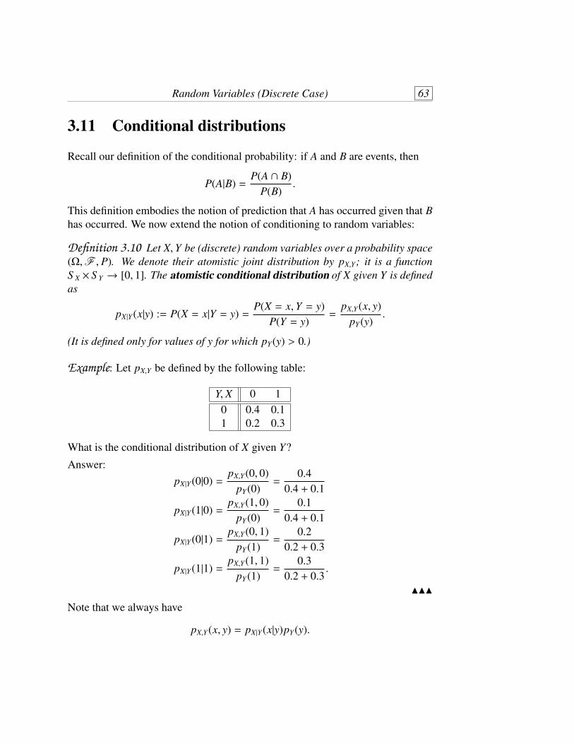
Random Variables (Discrete Case) 63
3.11 Conditional distributions
Recall our definition of the conditional probability: if A and B are events, then
P(A|B) =P(A ' B)
P(B).
This definition embodies the notion of prediction that A has occurred given that Bhas occurred. We now extend the notion of conditioning to random variables:
Definition 3.10 Let X,Y be (discrete) random variables over a probability space(",F , P). We denote their atomistic joint distribution by pX,Y; it is a functionS X # S Y 2 [0, 1]. The atomistic conditional distribution of X given Y is definedas
pX|Y(x|y) := P(X = x|Y = y) =P(X = x,Y = y)
P(Y = y)=
pX,Y(x, y)pY(y)
.
(It is defined only for values of y for which pY(y) > 0.)
Example: Let pX,Y be defined by the following table:
Y, X 0 10 0.4 0.11 0.2 0.3
What is the conditional distribution of X given Y?Answer:
pX|Y(0|0) =pX,Y(0, 0)
pY(0)=
0.40.4 + 0.1
pX|Y(1|0) =pX,Y(1, 0)
pY(0)=
0.10.4 + 0.1
pX|Y(0|1) =pX,Y(0, 1)
pY(1)=
0.20.2 + 0.3
pX|Y(1|1) =pX,Y(1, 1)
pY(1)=
0.30.2 + 0.3
.
!!!
Note that we always have
pX,Y(x, y) = pX|Y(x|y)pY(y).

64 Chapter 3
Summing over all y ! S Y ,
pX(x) =-
y!S Y
pX,Y(x, y) =-
y!S Y
pX|Y(x|y)pY(y),
which can be identified as the law of total probability formulated in terms ofrandom variables.
+ Exercise 3.10 True or false: every two random variables X,Y satisfy-
x!S X
pX|Y(x|y) = 1
-
y!S Y
pX|Y(x|y) = 1.
Example: Assume that the number of eggs laid by an insect is a Poisson variablewith parameter '. Assume, furthermore, that every eggs has a probability p todevelop into an insect. What is the probability that exactly k insects will survive?This problem has been previously given as an exercise. We will solve it now interms of conditional distributions. Let X be the number of eggs laid by the insect,and Y the number of survivors. We don’t even bother to (explicitly) write the prob-ability space, because we have all the needed data as distributions and conditionaldistributions. We know that X has a Poisson distribution with parameter ', i.e.,
pX(n) = e.''n
n!n = 0, 1, . . . ,
whereas the distribution of Y conditional on X is binomial,
pY |X(k|n) =2nk
3pk(1 . p)n.k k = 0, 1, . . . , n.
The distribution of the number of survivors Y is then
pY(k) =*-
n=0
pY |X(k|n)pX(n) =*-
n=k
2nk
3pk(1 . p)n.ke.'
'n
n!
= e.'('p)k
k!
*-
n=k
['(1 . p)]n.k
(n . k)!
= e.'('p)k
k!e'(1.p) = e.'p ('p)k
k!.
Thus, Y 6 Poi ('p). !!!

Random Variables (Discrete Case) 65
Example: Let X 6 Poi ('1) and Y 6 Poi ('2) be independent random variables.What is the conditional distribution of X given that X + Y = n?We start by writing things explicitly,
pX|X+Y(k|n) = P(X = k|X + Y = n)
=P(X = k, X + Y = n)
P(X + Y = n)
=pX,Y(k, n . k)
4nj=0 pX,Y( j, n . j)
.
At this point we use the fact that the variables are independent and their distribu-tions are known:
pX|X+Y(k|n) =e.'1
'k1
k! e.'2'n.k
2(n.k)!
4nj=0 e.'1
' j1
j! e.'2'n. j
2(n. j)!
=
0nk
1'k
1'n.k2
4nj=0
0nj
1' j
1'n. j2
=
0nk
1'k
1'n.k2
('1 + '2)n .
Thus, it is a binomial distribution with parameters n and '1/('1 + '2), which memay write as
[X conditional on X + Y = n] 6 B
2n,
'1
'1 + '2
3.
!!!
Conditional probabilities can be generalized to multiple variables. For example,
pX,Y |Z(x, y|z) := P(X = x,Y = y|Z = z) =pX,Y,Z(x, y, z)
pZ(z)
pX|Y,Z(x|y, z) := P(X = x|Y = y,Z = z) =pX,Y,Z(x, y, z)
pY,Z(y, z),
and so on.
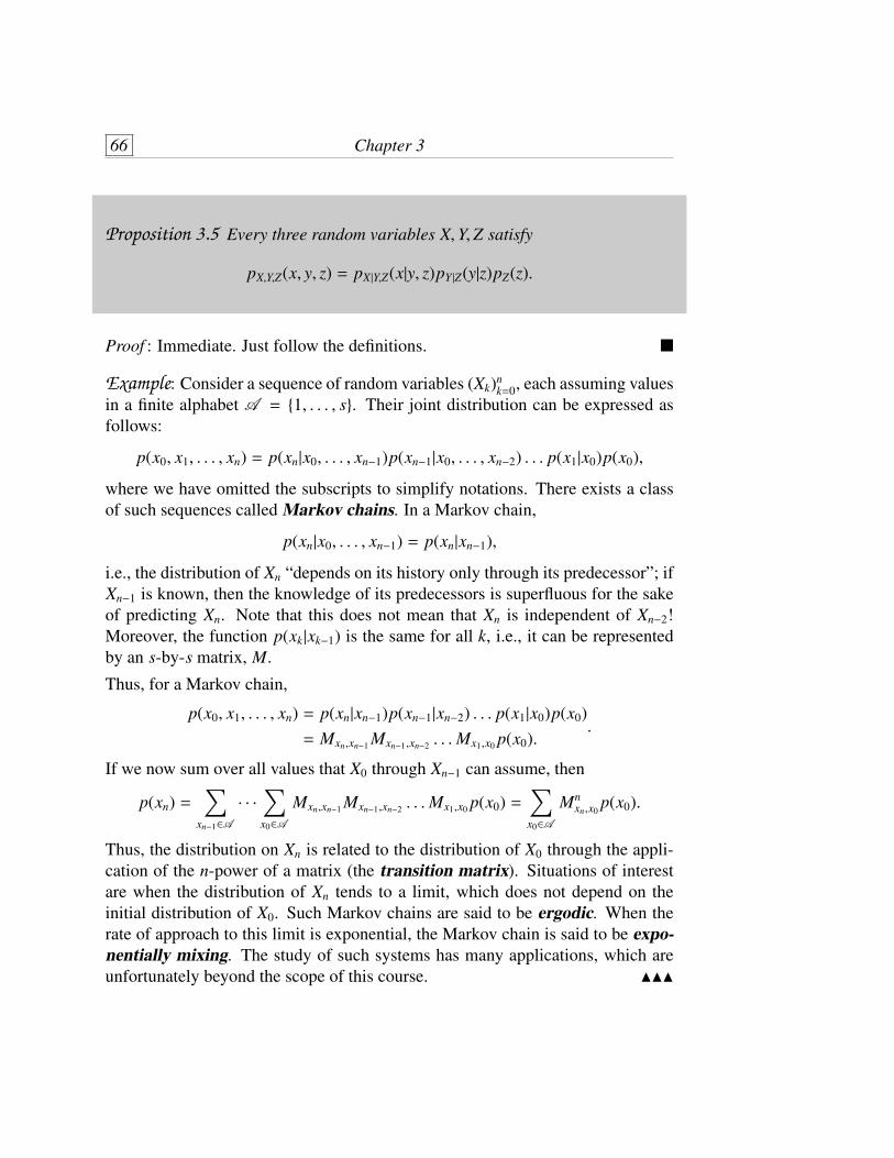
66 Chapter 3
Proposition 3.5 Every three random variables X,Y,Z satisfy
pX,Y,Z(x, y, z) = pX|Y,Z(x|y, z)pY |Z(y|z)pZ(z).
Proof : Immediate. Just follow the definitions. *
Example: Consider a sequence of random variables (Xk)nk=0, each assuming values
in a finite alphabet A = {1, . . . , s}. Their joint distribution can be expressed asfollows:
p(x0, x1, . . . , xn) = p(xn|x0, . . . , xn.1)p(xn.1|x0, . . . , xn.2) . . . p(x1|x0)p(x0),
where we have omitted the subscripts to simplify notations. There exists a classof such sequences called Markov chains. In a Markov chain,
p(xn|x0, . . . , xn.1) = p(xn|xn.1),
i.e., the distribution of Xn “depends on its history only through its predecessor”; ifXn.1 is known, then the knowledge of its predecessors is superfluous for the sakeof predicting Xn. Note that this does not mean that Xn is independent of Xn.2!Moreover, the function p(xk|xk.1) is the same for all k, i.e., it can be representedby an s-by-s matrix, M.Thus, for a Markov chain,
p(x0, x1, . . . , xn) = p(xn|xn.1)p(xn.1|xn.2) . . . p(x1|x0)p(x0)= Mxn,xn.1 Mxn.1,xn.2 . . .Mx1,x0 p(x0).
.
If we now sum over all values that X0 through Xn.1 can assume, then
p(xn) =-
xn.1!A· · ·-
x0!AMxn,xn.1 Mxn.1,xn.2 . . .Mx1,x0 p(x0) =
-
x0!AMn
xn,x0p(x0).
Thus, the distribution on Xn is related to the distribution of X0 through the appli-cation of the n-power of a matrix (the transition matrix). Situations of interestare when the distribution of Xn tends to a limit, which does not depend on theinitial distribution of X0. Such Markov chains are said to be ergodic. When therate of approach to this limit is exponential, the Markov chain is said to be expo-nentially mixing. The study of such systems has many applications, which areunfortunately beyond the scope of this course. !!!

Chapter 4
Expectation
Unregistered
!"#$% !&'(' )" *+ ,'-(!
,'-(' !(!./0 )% 1)01
#/ "#2#% &" *'+!
!3(# 1'0,) ,(/ 1)-'1
4.1 Basic definitions
Definition 4.1 Let X be a real-valued random variable over a discrete proba-bility space (",F , P). We denote the atomistic probability by p(!) = P({!}).The expectation or expected value of X is a real number denoted by E[X], anddefined by
E[X] :=-
!!"X(!) p(!).
It is an average over X(!), weighted by the probability p(!).
Comment: The expected value is only defined for random variables for which thesum converges absolutely. In the context of measure theory, the expectation is theintegral of X over the measure space (",F , P).

68 Chapter 4
The expected value of X can be rewritten in terms of the distribution of X:
E[X] =-
!!"X(!) p(!)
=-
x!S X
-
!!X.1(x)
X(!) p(!)
=-
x!S X
x-
!!X.1(x)
p(!)
=-
x!S X
x pX(x).
Thus, E[X] is the expected value of the identity function, X(x) = x, with respectto the probability space (S X,FX, PX).
Example: Let X be the outcome of a tossed die, what is the expected value of X?
In this case S = {1, . . . , 6} and pX(k) = 16 , thus
E[X] =6-
k=1
k · 16=
216.
!!!
Example: What is the expected value of X, which is a Bernoulli variable withpX(1) = p? Answer: p. !!!
Example: What is the expected value of X 6 B (n, p)?
E[X] =n-
k=0
k2nk
3pk(1 . p)n.k
=
n-
k=1
n!(n . k)!(k . 1)!
pk(1 . p)n.k
=
n.1-
k=0
n!(n . k . 1)!k!
pk+1(1 . p)n.k.1
= npn.1-
k=0
(n . 1)!(n . k . 1)!k!
pk(1 . p)n.k.1
= np.!!!

Expectation 69
Example: What is the expected value of X 6 Poi (')?
E[X] =*-
k=0
ke.''k
k!= e.'
*-
k=1
'k
(k . 1)!= e.'
*-
k=0
'k+1
k!= '.
!!!
Example: What is the expected value of X 6 Geo (p)?
E[X] =*-
k=1
kqk.1 p = pd
dq
*-
k=1
qk = pd
dq
2q
1 . q
3=
p(1 . q)2 =
1p.
If you don’t like this method, you can obtain the same result by noting that
E[X] = p +*-
k=2
kqk.1 p = p +*-
k=1
(k + 1)qk p = p +*-
k=1
qk p + qE[X],
i.e.,pE[X] = p +
pq1 . q
= 1.
!!!
+ Exercise 4.1 What is the expected value of the number of times one has totoss a die until getting a “3”? What is the expected value of the number of timesone has to toss two dice until getting a Shesh-Besh (6, 5)?
Example: Let X be a random variable assuming integer values and having anatomistic distribution of the form pX(k) = a/k2, where a is a constant. What is a?What is the expected value of X? !!!
What is the intuitive (until we prove some theorems) meaning of the expectedvalue? Suppose we repeat the same experiment many times and thus obtain asequence (Xk) of random variables that are mutually independent and have thesame distribution. Consider then the statistical average
Y =1n
n-
k=1
Xk =-
a!Sa
number of times the outcome was an
.
As n goes to infinity, this ratio tends to pX(a), and Y tends to E[X]. This heuristicargument lacks rigor (e.g., does it hold when S is an infinite set?), but should givemore insight into the definition of the expected value.

70 Chapter 4
4.2 The expected value of a function of a randomvariable
Example: Consider a random variable X assuming the values {0, 1, 2} and havinga distribution
x 0 1 2pX(x) 1/2 1/3 1/6
What is the expected value of the random variable X2?We need to follow the definition, construct the distribution pY of the random vari-able Y = X2, and then
E[X2] = E[Y] =-
y
y pY(y).
This is easy to do, because the distribution of Y is readily inferred from the distri-bution of X,
y 0 1 4pY(y) 1/2 1/3 1/6
thusE[Y] =
12· 0 + 1
3· 1 + 1
6· 4 = 1.
Note then that the arithmetic operation we do is equivalent to
E[X2] =-
x
x2 pX(x).
The question is whether it is generally true that for any function g : R2 R,
E[g(x)] =-
x
g(x) pX(x).
While this may seem intuitive, note that by definition,
E[g(x)] =-
y
y pg(X)(y).
!!!

Expectation 71
Theorem 4.1 (The unconscious statistician) Let X be a random variable withrange S X and atomistic distribution pX. Then, for any real valued function g,
E[g(X)] =-
x!S X
g(x) pX(x),
provided that the right-hand side is finite.
Proof : Let Y = g(X) and set S Y = g(S X) be the range set of Y . We need tocalculate E[Y], therefore we need to express the atomistic distribution of Y . Lety ! S Y , then
pY(y) = P({! : Y(!) = y}) = P({! : g(X(!)) = y})= P0{! : X(!) ! g.1(y)}
1,
where g.1(y) may be a subset of S X if g is not one-to-one. Thus,
pY(y) =-
S X=x!g.1(y)
pX(x).
The expected value of Y is then obtained by
E[Y] =-
y!S Y
y pY(y) =-
y!S Y
y-
S X=x!g.1(y)
pX(x)
=-
y!S Y
-
S X=x!g.1(y)
g(x)pX(x) =-
x!S X
g(x)pX(x).
*

72 Chapter 4
Comment: In a sense, this theorem is trivial. Had we followed the original defini-tion of the expected value, we would have had,
E[g(X)] =-
!!"g(X(!)) p(!)
=-
x!S X
-
!!X.1(x)
g(X(!)) p(!)
=-
x!S X
g(x)-
!!X.1(x)
p(!)
=-
x!S X
g(x) pX(x).
(This is the way I will prove it next time I teach this course...)
+ Exercise 4.2 Let X be a random variable and f , g be two real valued functions.Prove that
E[ f (X)g(X)] "0E[ f 2(X)]
11/2 0E[g2(X)]
11/2.
Hint: use the Cauchy inequality.
Example: The soccer club of Maccabbi Tel-Aviv plans to sell jerseys carrying thename of their star Eyal Berkovic. They must place their order at the beginningof the year. For every sold jersey they gain b Sheqels, but for every jersey thatremains unsold they lose % Sheqels. Suppose that the demand is a random variablewith atomistic distribution p( j), j = 0, 1, . . . . How many jerseys they need to orderto maximize their expected profit?
Let a be the number of jerseys ordered by the club, and X be the demand. The netprofit is then
g(X) =
@AABAAC
Xb . (a . X)% X = 0, 1, . . . , aab X > a
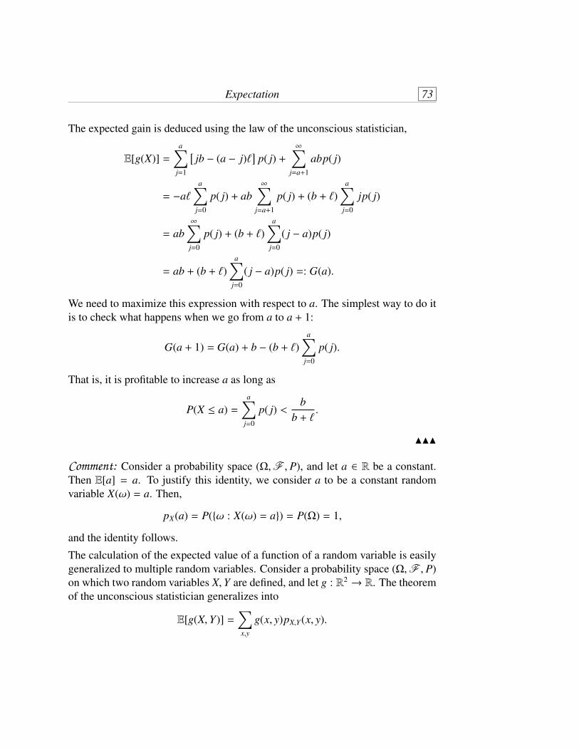
Expectation 73
The expected gain is deduced using the law of the unconscious statistician,
E[g(X)] =a-
j=1
Hjb . (a . j)%
Ip( j) +
*-
j=a+1
abp( j)
= .a%a-
j=0
p( j) + ab*-
j=a+1
p( j) + (b + %)a-
j=0
jp( j)
= ab*-
j=0
p( j) + (b + %)a-
j=0
( j . a)p( j)
= ab + (b + %)a-
j=0
( j . a)p( j) =: G(a).
We need to maximize this expression with respect to a. The simplest way to do itis to check what happens when we go from a to a + 1:
G(a + 1) = G(a) + b . (b + %)a-
j=0
p( j).
That is, it is profitable to increase a as long as
P(X " a) =a-
j=0
p( j) <b
b + %.
!!!
Comment: Consider a probability space (",F , P), and let a ! R be a constant.Then E[a] = a. To justify this identity, we consider a to be a constant randomvariable X(!) = a. Then,
pX(a) = P({! : X(!) = a}) = P(") = 1,
and the identity follows.The calculation of the expected value of a function of a random variable is easilygeneralized to multiple random variables. Consider a probability space (",F , P)on which two random variables X,Y are defined, and let g : R2 2 R. The theoremof the unconscious statistician generalizes into
E[g(X,Y)] =-
x,y
g(x, y)pX,Y(x, y).

74 Chapter 4
+ Exercise 4.3 Prove it.
Corollary 4.1 The expectation is a linear functional in the vector space of randomvariables: if X,Y are random variables over a probability space (",F , P) anda, b ! R, then
E[aX + bY] = aE[X] + bE[Y].
Proof : By the theorem of the unconscious statistician,
E[aX + bY] =-
x,y
(ax + by)pX,Y(x, y)
= a-
x
x-
y
pX,Y(x, y) + b-
y
y-
x
pX,Y(x, y)
= aE[X] + bE[Y].
*
This simple fact will be used extensively later on.
4.3 Moments
Definition 4.2 Let X be a random variable over a probability space. The n-thmoment of X is defined by
Mn[X] := E[Xn].If we denote the expected value of X by µ, then the n-th central moment of X isdefined by
Cn[X] := E[(X . µ)n].The second central moment of a random variable is called its variance, and it isdenoted by
Var[X] := E[(X . µ)2] = E[X2 . 2µX + µ2]= E[X2] . 2µE[X] + µ2 = E[X2] . (E[X])2.
(We have used the linearity of the expectation.) The square root of the variance iscalled the standard deviation, and is denoted by
$X =J
Var[X].

Expectation 75
The standard deviation is a measure of the (absolute) distance of the random vari-able from its expected value (or mean). It provides a measure of how “spread” thedistribution of X is.
Proposition 4.1 If Var[X] = 0, then X(!) = E[X] with probability one.
Proof : Let µ = E[X]. By definition,
Var[X] =-
x
(x . µ)2 pX(x).
This is a sum of non-negative terms. It can only be zero if pX(µ) = 1. *
Example: The second moment of a random variable X 6 B (n, p) is calculated asfollows:
E[X(X . 1)] =n-
k=0
k(k . 1)2nk
3pk(1 . p)n.k
=
n-
k=2
n!(n . k)!(k . 2)!
pk(1 . p)n.k
=
n.2-
k=0
n!(n . k . 2)!k!
pk+2(1 . p)n.k.2
= n(n . 1)p2.
Therefore,E[X2] = n(n . 1)p2 + E[X] = n(n . 1)p2 + np.
The variance of X is
Var[X] = n(n . 1)p2 + np . (np)2 = np(1 . p).
!!!
Example: What is the variance of a Poisson variable X 6 Poi (')? Recalling thata Poisson variable is the limit of a binomial variable with n 2 *, p 2 0, andnp = ', we deduce that Var[X] = '. !!!
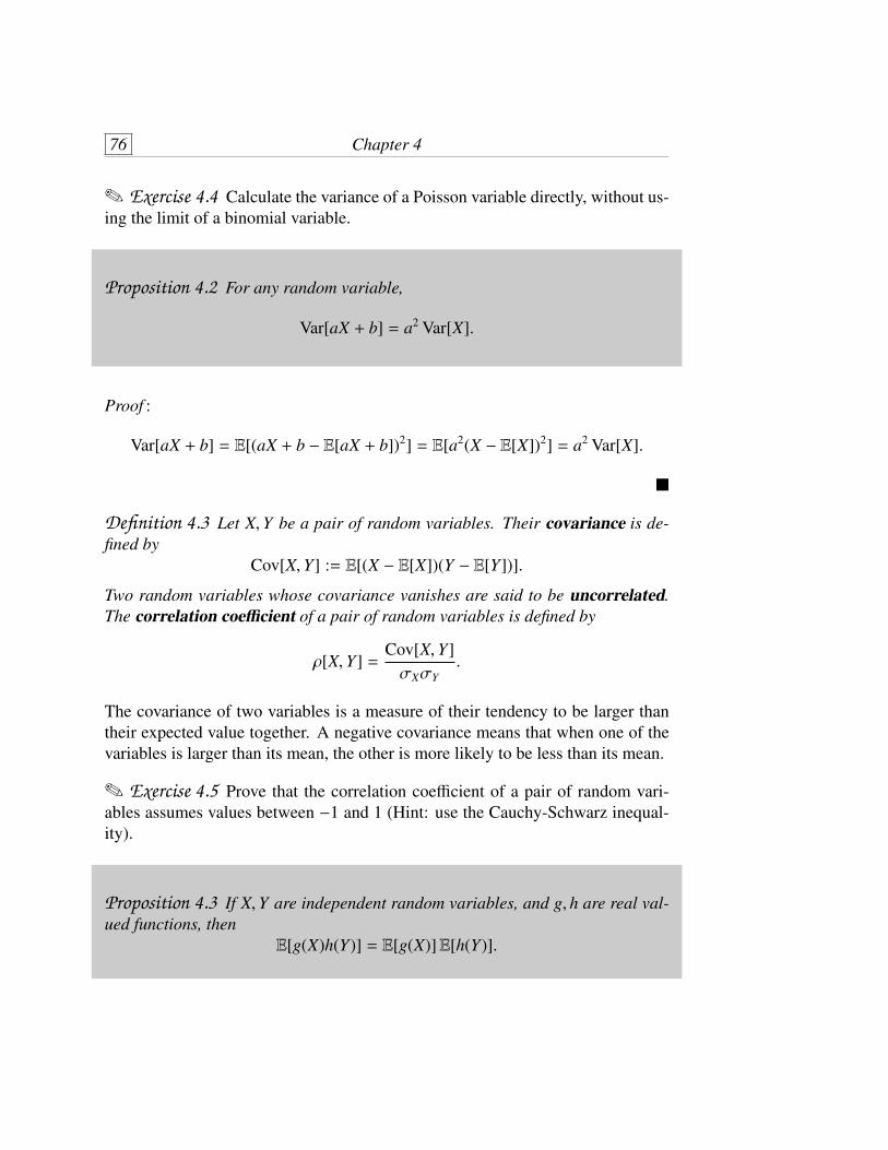
76 Chapter 4
+ Exercise 4.4 Calculate the variance of a Poisson variable directly, without us-ing the limit of a binomial variable.
Proposition 4.2 For any random variable,
Var[aX + b] = a2 Var[X].
Proof :
Var[aX + b] = E[(aX + b . E[aX + b])2] = E[a2(X . E[X])2] = a2 Var[X].
*
Definition 4.3 Let X,Y be a pair of random variables. Their covariance is de-fined by
Cov[X,Y] := E[(X . E[X])(Y . E[Y])].
Two random variables whose covariance vanishes are said to be uncorrelated.The correlation coe!cient of a pair of random variables is defined by
*[X,Y] =Cov[X,Y]$X$Y
.
The covariance of two variables is a measure of their tendency to be larger thantheir expected value together. A negative covariance means that when one of thevariables is larger than its mean, the other is more likely to be less than its mean.
+ Exercise 4.5 Prove that the correlation coe!cient of a pair of random vari-ables assumes values between .1 and 1 (Hint: use the Cauchy-Schwarz inequal-ity).
Proposition 4.3 If X,Y are independent random variables, and g, h are real val-ued functions, then
E[g(X)h(Y)] = E[g(X)]E[h(Y)].

Expectation 77
Proof : One only needs to apply the law of the unconscious statistician and use thefact that the joint distribution is the product of the marginal distributions,
E[g(X)h(Y)] =-
x,y
g(x)h(y)pX(x)pY(y)
=
'((((()-
x
g(x)pX(x)*+++++,
'(((((()-
y
h(y)pY(y)
*++++++,
= E[g(X)]E[h(Y)].
*
Corollary 4.2 If X,Y are independent then they are uncorrelated.
Proof : Obvious. *
Is the opposite statement true? Are uncorrelated random variables necessarilyindependent? Consider the following joint distribution:
X/Y .1 0 10 1/3 0 1/31 0 1/3 0
X and Y are not independent, because, for example, knowing that X = 1 impliesthat Y = 0. On the other hand,
Cov[X,Y] = E[XY] . E[X]E[Y] = 0 . 13· 0 = 0.
That is, zero correlation does not imply independence.
Proposition 4.4 For any two random variables X,Y,
Var[X + Y] = Var[X] + Var[Y] + 2 Cov[X,Y].

78 Chapter 4
Proof : Just do it! *
+ Exercise 4.6 Show that for any collection of random variables X1, . . . , Xn,
Var6777778
n-
k=1
Xk
9:::::; =
n-
k=1
Var[Xk] + 2-
i< j
Cov[Xi, Xj].
4.4 Using the linearity of the expectation
In this section we will examine a number of examples that make use of the additiveproperty of the expectation.
Example: Recall that we calculated the expected value of a binomial variable,X 6 B (n, p), and that we obtained E[X] = np. There is an easy way to obtain thisresult. A binomial variable can be represented as a sum of independent Bernoullivariables,
X =n-
k=1
Xk, Xk’s Bernoulli with success probability p.
By the additivity of the expectation,
E[X] =n-
k=1
E[Xk] = n · p.
The variance can be obtained by the same method. We have
Var[X] = n # Var[X1],
and it remains to verify that
Var[X1] = p(1 . p)2 + (1 . p)(0 . p)2 = (1 . p)(p(1 . p) + p2) = p(1 . p).
Note that the calculation of the expected value does not use the independenceproperty, whereas the calculation of the variance does. !!!
Example: A hundred dice are tossed. What is the expected value of their sum X?Let Xk be the outcome of the k-th die. Since E[Xk] = 21/6 = 7/2, we have byadditivity, E[X] = 100 # 7/2 = 350. !!!
Expectation 79
Example: Consider again the problem of the inattentive secretary who puts nletters randomly into n envelopes. What is the expected number of letters thatreach their destination?Define for k = 1, . . . , n the Bernoulli variables,
Xk =
@AABAAC
1 the k-th letter reached its destination0 otherwise.
Clearly, pXk(1) = 1/n. If X is the number of letters that reached their destination,then X =
4nk=1 Xk, and by additivity,
E[X] = n # 1n= 1.
We then proceed to calculate the variance. We’ve already seen that for the Bernoullivariable with parameter p the variance equals p(1. p). In this case, the Xk are notindependent therefore we need to calculate their covariance. The variable X1X2 isalso a Bernoulli variable, with parameter 1/n(n . 1), so that
Cov[X1, X2] =1
n(n . 1). 1
n2 .
Putting things together,
Var[X] = n # 1n
21 . 1
n
3+ 22n2
3#2
1n(n . 1)
. 1n2
3
=
21 . 1
n
3+ n(n . 1)
21
n(n . 1). 1
n2
3= 1.
Should we be surprised? Recall that X tends as n2 * to a Poisson variable withparameter ' = 1, so that we expect that in this limit E[X] = Var[X] = 1. It turnsout that this result holds exactly for every finite n. !!!
+ Exercise 4.7 In an urn are N white balls and M black balls. n balls are drawnrandomly. What is the expected value of the number of white balls that weredrawn? (Solve this problem by using the additivity of the expectation.)
Example: Consider a randomized deck of 2n cards, two of type “1”, two of type“2”, and so on. m cards are randomly drawn. What is the expected value of thenumber of pairs that will remain intact? (This problem was solved by Daniel

80 Chapter 4
Bernoulli in the context of the number of married couples remaining intact afterm deaths.)We define Xk to be a Bernoulli variable taking the value 1 if the k-th couple re-mains intact. We have
E[Xk] = pXk(1) =
02n.2
m
1
02nm
1 =(2n . m)(2n . m . 1)
2n(2n . 1).
The desired result is n times this number. !!!
Example: Recall the coupon collector: there are n di#erent coupons, and eachturn there is an equal probability to obtain any coupon. What is the expected valueof the number of coupons that need to be collected before obtaining a completeset?Let X be the number of coupons that need to be collected and Xk be the numberof coupons that need to be collected from the moment that we had k di#erentcoupons to the moment we have k + 1 di#erent coupons. Clearly,
X =n.1-
k=0
Xk.
Now, suppose we have k di#erent coupons. Every new coupon can be viewed as aBernoulli experiment with success probability (n . k)/n. Thus, Xk is a geometricvariable with parameter (n . k)/n, and E[Xk] = n/(n . k). Summing up,
E[X] =n.1-
k=0
nn . k
= nn-
k=1
1k/ n log n.
!!!
+ Exercise 4.8 Let X1, . . . , Xn be a sequence of independent random variablesthat have the same distribution. We denote E[X1] = µ and Var[X1] = $2. Find theexpected value and the variance of the empirical mean
S n =1n
n-
k=1
Xk.
We conclude this section with a remark about infinite sums. First a simple lemma:

Expectation 81
Lemma 4.1 Let X be a random variable. If X(!) , a (with probability one) thenE[X] , a. Also,
E[|X|] , |E[X]|.
Proof : The first result follows from the definition of the expectation. The secondresult follows from the inequality
KKKKKKK
-
x
x pX(x)
KKKKKKK"-
x
|x| pX(x).
*
Theorem 4.2 Let (Xn) be an infinite sequence of random variables such that
*-
n=1
E[|Xn|] < *.
Then,
E
6777778*-
n=1
Xn
9:::::; =
*-
n=1
E[Xn].
Proof : TO BE COMPLETED. *
The following is an application of the above theorem. Let X be a random variableassuming positive integer values and having a finite expectation. Define for everynatural i,
Xi(!) =
@AABAAC
1 i " X(!)0 otherwise
Then,*-
i=1
Xi(!) =-
i"X(!)
1 = X(!).

82 Chapter 4
Now,
E[X] =*-
i=1
E[Xi] =*-
i=1
P({! : X(!) , i}).
4.5 Conditional expectation
Definition 4.4 Let X,Y be random variables over a probability space (",F , P).The conditional expectation of X given that Y = y is defined by
E[X|Y = y] :=-
x
x pX|Y(x|y).
Note that this definition makes sense because pX|Y(·|y) is an atomistic distributionon S X.
Example: Let X,Y 6 B (n, p) be independent. What is the conditional expecta-tion of X given that X + Y = m?To answer this question we need to calculate the conditional distribution pX|X+Y .Now,
pX|X+Y(k|m) =P(X = k, X + Y = m)
P(X + Y = m)=
P(X = k,Y = m . k)P(X + Y = m)
,
with k " m, n. We know what the numerator is. For the denominator, we real-ize that the sum of two binomial variables with parameters (n, p) is a binomialvariable with parameters (2n, p) (think of two independent sequences of Bernoullitrials added up). Thus,
pX|X+Y(k|m) =
0nk
1pk(1 . p)n.k
0n
m.k
1pm.k(1 . p)n.m+k
02nm
1pm(1 . p)2n.m
=
0nk
10n
m.k
1
02nm
1 .
The desired result is
E[X|X + Y = m] =min(m,n)-
k=0
k
0nk
10n
m.k
1
02nm
1 .
It is not clear how to simplify this expression. A useful trick is to observe thatpX|X+Y(k|m) with m fixed is the probability of obtaining k white balls when one

Expectation 83
draws m balls from an urn containing n white balls and n black balls. Since everyball is white with probability 1/2, by the additivity of the expectation, the expectednumber of white balls is m/2.Now that we know the result, we may see that we could have reached it muchmore easily. By symmetry,
E[X|X + Y = m] = E[Y |X + Y = m],
hence, by the linearity of the expectation,
E[X|X + Y = m] =12E[X + Y |X + Y = m] =
m2.
In particular, this result holds whatever is the distribution of X,Y (as long as it isthe same). !!!
We now refine our definition of the conditional expectation:
Definition 4.5 Let X(!),Y(!) be random variables over a probability space (",F , P).The conditional expectation of X given Y is a random variable Z(!), which is acomposite function of Y(!), i.e., Z(!) = +(Y(!)), and
+(y) := E[X|Y = y].
Another way to write it is:
E[X|Y](!) := E[X|Y = y]y=Y(!).
That is, having performed the experiment, we are given only Y(!), and the randomvariable E[X|Y](!) is the expected value of X(!) now that we know Y(!).
Proposition 4.5 For every two random variables X,Y,
E[E[X|Y]] = E[X].
Proof : What does the proposition say? That-
!!"E[X|Y](!) p(!) =
-
!!"X(!) p(!).
84 Chapter 4
Since E[X|Y](!) is a composite function of Y(!) we can use the law of the uncon-scious statistician to rewrite this as
-
y
E[X|Y = y] pY(y) =-
x
x pX(x).
Indeed,-
y
E[X|Y = y] pY(y) =-
y
-
x
x pX|Y(x|y)pY(y)
=-
y
-
x
x pX,Y(x, y) = E[X].
*
This simple proposition is quite useful. It states that the expected value of X canbe computed by averaging over its expectation conditioned over another variable.
Example: A miner is inside a mine, and doesn’t know which of three possibletunnels will lead him out. If he takes tunnel A he will be out within 3 hours. If hetakes tunnel B he will be back to the same spot after 5 hours. If he takes tunnel Che will be back to the same spot after 7 hours. He chooses the tunnel at randomwith equal probability for each tunnel. If he happens to return to the same spot,the poor thing is totally disoriented, and has to redraw his choice again with equalprobabilities. What is the expected time until he finds the exit?The sample space consists of infinite sequences of ”BCACCBA...”, with the stan-dard probability of independent repeated trials. Let X(!) be the exit time and Y(!)be the label of the first door he chooses. By the above proposition,
E[X] = E[E[X|Y]]= E[X|Y = A] pY(A) + E[X|Y = B] pY(B) + E[X|Y = C] pY(C)
=13
(3 + E[X|Y = B] + E[X|Y = C]) .
What is E[X|Y = B]? If the miner chose tunnel B, then he wandered for 5 hours,and then faced again the original problem, independently of his first choice. Thus,
E[X|Y = B] = 5 + E[X] and similarly E[X|Y = C] = 7 + E[X].
Substituting, we get
E[X] = 1 +13
(5 + E[X]) +13
(7 + E[X]) .
This equation is easily solved, E[X] = 15. !!!

Expectation 85
Example: Consider a sequence of independent Bernoulli trials with success prob-ability p. What is the expected number of trials until one obtains two 1’s in arow?Let X(!) be the number of trials until two 1’s in a row, and let Yj(!) be theoutcome of the j-th trial. We start by writing
E[X] = E[E[X|Y1]] = pE[X|Y1 = 1] + (1 . p)E[X|Y1 = 0].
By the same argument as above,
E[X|Y1 = 0] = 1 + E[X].
Next, we use a simple generalization of the conditioning method,
E[X|Y1 = 1] = pE[X|Y1 = 1,Y2 = 1] + (1 . p) E[X|Y1 = 1,Y2 = 0].
Using the fact that
E[X|Y1 = 1,Y2 = 1] = 2 and E[X|Y1 = 1,Y2 = 0] = 2 + E[X],
we finally obtain an implicit equation for E[X]:
E[X] = pH2p + (1 . p)(2 + E[X])
I+ (1 . p)(1 + E[X]),
from which we readily obtain
E[X] =1 + p
p2 .
We can solve this same problem di#erently. We view the problem in terms ofa three-state space: one can be in the initial state (having to produce two 1’s ina row), be in state after a single 1, or be in the terminal state after two 1’s in arow. We label these states S 0, S 1, and S 2. Now every sequence of successes andfailures implies a trajectory on the state space. That is, we can replace the originalsample space of sequences of zero-ones by a sample space of sequences of statesS j. This defined a new compound experiment, with transition probabilities thatcan be represented as a graph:
!"#$
!"#$
!"#$%&'(
S 0 S 1 S 2! ! !p p
1 . p 1 . p

86 Chapter 4
Let now X(!) be the number of steps until reaching state S 2. The expected valueof X depends on the initial state. The graph suggests the following relations,
E[X|S 0] = 1 + pE[X|S 1] + (1 . p)E[X|S 0]E[X|S 1] = 1 + pE[X|S 2] + (1 . p)E[X|S 0]E[X|S 2] = 0
It is easily checked that E[X|S 0] = (1 + p)/p2. !!!
I AM NOT SATISFIED WITH THE WAY THIS IS EXPLAINED. REQUIRESELABORATION.
+ Exercise 4.9 Consider a sequence of independent Bernoulli trials with suc-cess probability p. What is the expected number of trials until one obtains three1’s in a row? four 1’s in a row?
+ Exercise 4.10 A monkey types randomly on a typing machine. Each characterhas a probability of 1/26 of being each of the letters of the alphabet, independentlyof the other. What is the expected number of characters that the monkey will typeuntil generating the string ”ABCD”? What about the string ”ABAB”?
The following paragraphs are provided for those who want to know more.
The conditional expectation E[X|Y](!) plays a very important role in probability theory.Its formal definition, which remains valid in the general case (i.e., uncountable spaces),is somewhat more involved than that presented in this section, but we do have all thenecessary background to formulate it. Recall that a random variable Y(!) generates a$-algebra of events (a sub-$-algebra of F ),
F - $(Y) :=!Y.1(A) : A ! FY
".
Let + be a real valued function defined on S Y , and define a random variable Z(!) =+(Y(!)). The $-algebra generated by Z is
$(Z) :=!Z.1(B) : B ! FZ
"=!Y.1(+.1(B)) : B ! FZ
"& $(Y).
That is, the $-algebra generated by a function of a random variable is contained in the$-algebra generated by this random variable. In fact, it can be shown that the oppositeis true. If Y,Z are random variables and $(Z) & $(Y), then Z can be expressed as acomposite function of Y .
Recall now our definition of the conditional expectation,
E[X|Y](!) = E[X|Y = y]y=Y(!) =-
xx pX|Y (x|Y(!)) =
-
xx
pX,Y (x,Y(!))pY (Y(!))
.
Expectation 87
Let A ! F be any event in $(Y), that is, there exists a B ! FY for which Y.1(B) = A.Now,
-
!!AE[X|Y](!) p(!) =
-
!!A
-
xx
pX,Y (x,Y(!))pY (Y(!))
p(!)
=-
xx-
!!A
pX,Y (x,Y(!))pY (Y(!))
p(!)
=-
xx-
y!B
-
!!Y.1(y)
pX,Y (x, y)pY (y)
p(!)
=-
xx-
y!B
pX,Y (x, y)pY (y)
-
!!Y.1(y)
p(!)
=-
xx-
y!B
pX,Y (x, y).
On the other hand,-
!!AX(!) p(!) =
-
y!B
-
!!Y.1(y)
X(!) p(!)
=-
x
-
y!B
-
{!:(X(!),Y(!))=(x,y)}X(!) p(!)
=-
xx-
y!B
-
{!:(X(!),Y(!))=(x,y)}p(!)
=-
xx-
y!B
pX,Y (x, y).
That is, for every A ! $(Y),-
!!AE[X|Y](!) p(!) =
-
!!AX(!) p(!).
This property is in fact the standard definition of the conditional expectation:
Definition 4.6 Let X,Y be random variables over a probability space (",F , P). Theconditional expectation of X given Y is a random variable Z satisfying the following twoproperties: (1) $(Z) & $(Y), (2) For every A ! $(Y)
-
!!AZ(!) p(!) =
-
!!AX(!) p(!).
It can be proved that there exists a unique random variable satisfying these properties.

88 Chapter 4
4.6 The moment generating function
Definition 4.7 Let X be a discrete random variable. Its moment generatingfunction MX(t) is a real-valued function defined by
MX(t) := E[etX] =-
x
etx pX(x).
Example: What is the moment generating function of a binomial variable X 6B (n, p)?
MX(t) =n-
k=1
etk2nk
3pk(1 . p)n.k = (1 . p + et p)n.
!!!
Example: What is the moment generating function of a Poisson variable X 6Poi (')?
MX(t) =*-
k=0
etke.''k
k!= e'(e
t.1).
!!!
What are the uses of the moment generating function? Note that
MX(0) = 1M?X(0) = E[X]M??X (0) = E[X2],
and in general, the k-th derivative evaluated at zero equals to the k-th moment.
Example: Verify that we get the correct moments for the binomial and Poissonvariables !!!
Comment: The moment-generating function is the Laplace transform of theatomistic distribution. It has many uses, which are however beyond the scopeof this course.

Chapter 5
Random Variables (ContinuousCase)
So far, we have purposely limited our consideration to random variables whoseranges are countable, or discrete. The reason for that is that distributions on count-able spaces are easily specified by means of the atomistic distribution. The con-struction of a distribution on an uncountable space is only done rigorously withinthe framework of measure theory. Here, we will only provide limited tools thatwill allow us to operate with such variables.
5.1 Basic definitions
Definition 5.1 Let (",F , P) be a probability space. A real-valued function"2R is called a continuous random variable, if there exists a non-negative real-valued integrable function fX(x), such that
P({! : X(!) " a}) = FX(a) =L a
.*fX(x) dx.
The function fX is called the probability density function (pdf) of X.
Comment: Recall that a random variable has a $-algebra of events FX associatedwith its range (here R), and we need X.1(A) ! F for all A ! FX. What is asuitable $-algebra for R? These are precisely the issues that we sweep under
90 Chapter 5
the carpet (well, I can still tell you that it is the $-algebra generated by all opensubsets of the line).Thus, a continuous random variable is defined by its pdf. Since a random variableis by definition defined by its distribution PX, we need to show that the pdf definesthe distribution uniquely. Since we don’t really know how to define distributionswhen we don’t even know the set of events, this cannot really be achieved. Yet,we can at least show the following properties:(1) For every segment (a, b],
PX((a, b]) = FX(b) . FX(a) =L b
afX(x) dx.
(2) For every A expressible as a countable union of disjoint (aj, bj],
PX(A) =L
AfX(x) dx.
(3) Normalization, L
R
fX(x) dx = 1.
(4) The distribution of closed sets follows from the continuity of the probability,
PX([a, b]) = P>limn2*
(a . 1n , b]?= lim
n2*
L b
a.1/nfX(x) dx = PX((a, b]).
(5) As a result, PX({a}) = 0 for every a ! R, as
P({a}) = PX([a, b]) . PX((a, b]).
Comment: We may consider discrete random variables as having a pdf which is asum of ,-functions.
Example: The random variable X has a pdf of the form
fX(x) =
@AABAAC
2C(2x . x2) 0 " x " 20 otherwise
.
What is the value of the constant C and what is the probability that X(!) > 1?
Random Variables (Continuous Case) 91
The constant is obtained by normalization,
1 = 2CL 2
0(2x . x2) dx = 2C
24 . 8
3
3=
8C3.
Then,
P(X > 1) = 2CL 2
1(2x . x2) dx =
12.
!!!
5.2 The uniform distribution
Definition 5.2 A random variable X is called uniformly distributed in [a, b],denoted X 6 U (a, b), if its pdf is given by
fX(x) =
@AABAAC
1b.a a " x " b0 otherwise
.
Example: Buses are arriving at a station every 15 minutes. A person arrives atthe station at a random time, uniformly distributed between 7:00 and 7:30. Whatis the probability that he has to wait less than 5 minutes?Let X(!) be the arrival time (in minutes past 7:00), and Y(!) the time he has towait. We know that X 6 U (0, 30). Now,
P(Y < 5) = P({X = 0} % {10 " X < 15} % {25 " X < 30}) = 0 +5
30+
530=
13.
!!!
Example: Bertrand’s paradox: consider a random chord of a circle. What is theprobability that the chord is longer than the side of an equilateral triangle inscribedin that circle?The “paradox” stems from the fact that the answer depends on the way the randomchord is selected. One possibility is to take the distance of the chord from thecenter of the circle r to be U (0,R). Since the chord is longer than the side of theequilateral triangle when r < R/2, the answer is 1/2. A second possibility is totake the angle " between the chord and the tangent to the circle to be U (0, #). Thechord is longer than the side of the triangle when #/3 < " < 2#/3, in which casethe answer is 1/3.
!!!

92 Chapter 5
5.3 The normal distribution
Definition 5.3 A random variable X is said to be normally distributed withparameters µ,$2, denoted by X 6 N(µ,$2), if its pdf is
fX(x) =18
2#$2exp2. (x . µ)2
2$2
3.
X is called a standard normal variable if µ = 0 and $2 = 1.
+ Exercise 5.1 Show that the pdf of a normal variable N(µ,$2) is normalized.
Proposition 5.1 Let X 6 N(µ,$2) and set Y = aX + b, where a > 0. Then
Y 6 N(aµ + b, a2$2).
Proof : At this point, where we don’t know how to change variables, we simplyoperate on the distribution function of Y ,
FY(y) = P(Y " y) = P(X " a.1(y . b))
=18
2#$2
L a.1(y.b)
.*exp2. (x . µ)2
2$2
3dx
=1/a82#$2
L y
.*exp2. (a.1(u . b) . µ)2
2$2
3du
=18
2#a2$2
L y
.*exp2. (u . b . aµ)2
2a2$2
3du,
where we have changed variables, x = a.1(u . b). *
Corollary 5.1 If X 6 N(µ,$2) then (X . µ)/$ is a standard normal variable.

Random Variables (Continuous Case) 93
Notation: The distribution function of a standard normal variable will be denotedby %(x),
%(x) :=182#
L x
.*e.y2/2 dy.
(This function is closely related to Gauss’ error function).
The importance of the normal distribution stems from the central limit theorem,which we will encounter later on. The following theorem is an instance of thecentral limit theorem for a particular case:
Theorem 5.1 (DeMoivre-Laplace) Let (Xn) be a sequence of independentBernoulli variables with parameter p and set
Yn :=Xn . pJ
p(1 . p).
(The variables Yn have zero expectation and unit variance.) Set then
S n :=18n
n-
k=1
Yk.
Then S n tends, as n2 *, to a standard normal variable in the sense that
limn2*
P (a " S n " b) = %(b) . %(a).
Comment: This theorem states that the sequence of random variables S n con-verges to a standard normal variable in distribution, or in law.
Proof : The event {a " S n " b} can be written as
@AABAACnp +
Jnp(1 . p) a "
n-
k=1
Xk " np +J
np(1 . p) b
MAANAAO ,

94 Chapter 5
and the sum over Xk is a binomial variable B (n, p). Thus, the probability of thisevent is
P (a " S n " b) =np+8
np(1.p) b-
k=np+8
np(1.p) a
2nk
3pk(1 . p)n.k.
(We will ignore the fact that limits are integer as the correction is negligible asn 2 *.) As n becomes large (while p remains fixed), n, k, and n . k becomelarge, hence we use Stirling’s approximation,
2nk
36
82#n nne.n
82#k kke.k
82#(n . k) (n . k)n.ke.(n.k)
,
and so 2nk
3pk(1 . p)n.k 6
Pn
2#k(n . k)
>npk
?k 2n(1 . p)n . k
3n.k
,
where, as usual, the 6 relation means that the ratio between the two sides tends toone as n 2 *. The summation variable k takes values that are of order O(
8n)
around np. This suggests a change of variables, k = np+J
np(1 . p) m, where mvaries from a to b in units of &m = [np(1 . p)].1/2.Consider the first term in the above product. As n2 *,
limn2*
1&m
Pn
2#k(n . k)= lim
n2*
8n8
2#n
Jp(1 . p)
8(k/n)(1 . k/n)
=182#.
Consider the second term, which we can rewrite as>np
k
?k=
2np
np + r8
n
3np+r8
n
,
where r =J
p(1 . p) m. To evaluate the n 2 * limit it is easier to look at thelogarithm of this expression, whose limit we evaluate using Taylor’s expansion,
log>np
k
?k= (np + r
8n) log
21 +
rp
n.1/23.1
= (np + r8
n) log21 . r
pn.1/2 +
r2
p2 n.13+ l.o.t
= (np + r8
n)2. r
pn.1/2 +
r2
2p2 n.13+ l.o.t
= .r8
n . r2
2p= .r
8n . 1
2(1 . p)m2 + l.o.t.

Random Variables (Continuous Case) 95
Similarly,
log2n(1 . p)
n . k
3n.k
= r8
n . 12
pm2 + l.o.t.
Combining the two together we have
limn2*
log677778>np
k
?k 2n(1 . p)n . k
3n.k9::::; = .12
m2.
Thus, as n2 * we have
limn2*
P (a " S n " b) = limn2*
182#
b-
m=a
e.m2/2 &m = %(b) . %(a),
which concludes the proof. *
A table of the values of %(x) is all that is needed to compute probabilities forgeneral normal variables. Indeed, if X 6 N(µ,$2), then
FX(x) = P(X " x) = P>X . µ$" x . µ$
?= %> x . µ$
?.
Example: The duration of a normal pregnancy (in days) is a normal variableN (270, 100). A sailor’s wife gave birth to a baby. It turns out that her husbandwas on the go during a period that started 290 days before the delivery and ended240 days before the delivery. What is the probability that the baby was conceivedwhile he was at home?Let X be the actual duration of the pregnancy. The question is
P ({X > 290} % {X < 240}) =?,
which we solve as follows,
P ({X > 290} % {X < 240}) = P2F
X . 27010
> 2G%F
X . 27010
< .3G3
=182#
L .3
.*e.y2/2 dy +
182#
L *
2e.y2/2 dy
= %(.3) + [1 . %(2)] = 0.241.
(It is with great relief that we learn that after having completed this calculation,the sailor decided not to slaughter his wife.) !!!

96 Chapter 5
Example: A fair coin is tossed 40 times. What is the probability that the numberof Heads equals exactly 20?Since the number of heads is a binomial variable, the answer is
24020
3 212
320 212
320
= 0.1268...
We can also approximate the answer using the DeMoivre-Laplace theorem. In-deed, the random variable
X . 40 # 12Q
40 # 12 # (1 . 1
2 )/ N (0, 1) .
The number of heads is a discrete variable, whereas the normal distribution refersto a continuous one. We will approximate the probability that the number of headsbe 20 by the probability that it is, in a continuous context, between 19.5 and 20.5,i.e., that
|X . 20|810
" 128
10,
and
P2
128
10" X . 208
10" 1
28
10
3/ 22%
21
28
10
3. %(0)
3= 0.127...
!!!
5.4 The exponential distribution
Definition 5.4 A random variable X is said to be exponentially distributed withparameter ', denoted X 6 Exp ('), if its pdf is
fX(x) =
@AABAAC' e.'x x , 00 x < 0
.
The corresponding distribution function is
FX(x) =
@AABAAC
1 . e.'x x , 00 x < 0
.

Random Variables (Continuous Case) 97
An exponential distribution is a suitable model in many situations, like the timeuntil the next earthquake.
Example: Suppose that the duration of a phone call (in minutes) is a randomvariable Exp (1/10). What is the probability that a given phone call lasts morethan 10 minutes? The answer is
P(X > 10) = 1 . Fx(10) = e.10/10 / 0.368.
Suppose we know that a phone call has already lasted 10 minutes. What is theprobability that it will last at least 10 more minutes. The perhaps surprising answeris
P(X > 20|X > 10) =P(X > 20, X > 10)
P(X > 10)=
e.2
e.1 = e.1.
More generally, we can show that for every t > s,
P(X > t|X > s) = P(X > t . s).
A random variable satisfying this property is called memoryless. !!!
Proposition 5.2 A random variable that satisfies
P(X > t|X > s) = P(X > t . s) for all t > s > 0
is exponentially distributed.
Proof : It is given that
P(X > t, X > s)P(X > s)
= P(X > t . s),
or in terms of the distribution function,1 . FX(t)1 . FX(s)
= 1 . FX(t . s).
Let g(t) = 1 . FX(t), then for all t > s,
g(t) = g(s)g(t . s),
and the only family of functions satisfying this property is the exponentials. *

98 Chapter 5
5.5 The Gamma distribution
The Gamma function is defined by
$(x) =L *
0tx.1e.t dt
for x > 0. This function is closely related to factorials since $(1) = 1 and byintegration by parts,
$(n + 1) =L *
0tne.t dt = n
L *
0tn.1e.t dt = n$(n),
hence $(n + 1) = n! for integer n. A random variable X is said to be Gamma-distributed with parameters r, ' if it assumes positive values and
fX(x) ='r
$(r)xr.1e.'x.
We denote it by X 6 Gamma (r, '). This is a normalized pdf sinceL *
0fX(x) dx =
1$(r)
L *
0('x)r.1e.'x d('x) = 1.
Note that for r = 1 we get the pdf of an exponential distribution, i.e.,
Gamma (1, ') 6 Exp (') .
The significance of the Gamma distribution will be seen later on in this chapter.
5.6 The Beta distribution
A random variable assuming values in [0, 1] is said to have the Beta distributionwith parameters K, L > 0, i.e., X 6 Beta (K, L), if it has the pdf
fX(x) =$(K + L)$(K)$(L)
xK.1(1 . x)L.1.
Random Variables (Continuous Case) 99
5.7 Functions of random variables
In this section we consider the following problem: let X be a continuous randomvariable with pdf fX(x). Let g be a real-valued function and Y(!) = g(X(!)). Whatis the distribution of Y?
Example: Let X 6 U (0, 1). What is the distribution of Y = Xn?The random variable Y , like X, assumes values in the interval [0, 1]. Now,
FY(y) = P(Y " y) = P(Xn " y) = P(X " y1/n) = FX(y1/n),
where we used the monotonicity of the power function for positive arguments. Inthe case of a uniform distribution,
FX(x) =L x
.*fX(x) =
@AAAAABAAAAAC
0 x < 0x 0 " x " 11 x > 1
.
Thus,
FY(y) =
@AAAAABAAAAAC
0 y < 0y1/n 0 " y " 11 y > 1
.
Di#erentiating,
fY(y) =dFY(y)
dy=
@AABAAC
1n y1/n.1 0 " y " 10 otherwise
.
!!!
Example: Let X be a continuous random variable with pdf fX(x). What is thedistribution of Y = X2.The main di#erence with the previous exercise is that X may possibly assume bothpositive and negative values, in which case the square function is non-monotonic.Thus, we need to proceed with more care,
FY(y) = P(Y " y) = P(X2 " y)= P(X , .8y, X " 8y)= FX(
8y) . FX(.8y).

100 Chapter 5
Di#erentiating, we get the pdf
fY(y) =fX(8y) + fX(.8y)
28y.
!!!
With these preliminaries, we can formulate the general theorem:
Theorem 5.2 Let X be a continuous random variable with pdf fX(x). Let g bea strictly monotonic, di!erentiable function and set Y(!) = g(X(!)). Then therandom variable Y has a pdf
fY(y) =
@AABAAC
KKK(g.1)?(y)KKK fX(g.1(y)) y is in the range of g(X)
0 otherwise.
Comment: If g is non-monotonic then g.1(y) may be set-valued and the aboveexpression has to be replaced by a sum over all “branches” of the inverse function:
-
g.1(y)
KKK(g.1)?(y)KKK fX(g.1(y)).
Proof : Consider the case where g is strictly increasing. Then, g.1 exists, and
FY(y) = P(Y " y) = P(g(X) " y) = P(X " g.1(y)) = FX(g.1(y)),
and upon di#erentiation,
fY(y) =ddy
FX(g.1(y)) = (g.1)?(y) fX(g.1(y)).
The case where g is strictly decreasing is handled similarly. *
Random Variables (Continuous Case) 101
The inverse transformation method An application of this formula is the fol-lowing. Suppose that you have a computer program that generates a random vari-able X 6 U (0, 1). How can we use it to generate a random variable with distribu-tion function F? The following method is known as the inverse transformationmethod.If F is strictly increasing (we know that it is at least non-decreasing), then we candefine
Y(!) = F.1(X(!)).
Note that F.1 maps [0, 1] onto the entire real line, while X has range [0, 1]. More-over, FX(x) is the identity on [0, 1]. By the above formula,
FY(y) = FX(F(y)) = F(y).
Example: Suppose we want to generate an exponential variable Y 6 Exp ('), inwhich case F(y) = 1 . e.'y. The inverse function is F.1(x) = . 1
' log(1 . x), i.e.,an exponential variable is generated by setting
Y(!) = .1'
log(1 . X(!)).
In fact, since 1 . X has the same distribution as X, we may equally well takeY = .'.1 log X.
!!!
5.8 Multivariate distributions
We proceed to consider joint distributions of multiple random variables. The treat-ment is fully analogous to that for discrete variables.
Definition 5.5 A pair of random variables X,Y over a probability space (",F , P)is said to have a continuous joint distribution if there exists an integrable non-negative bi-variate function fX,Y(x, y) (the joint pdf) such that for every (measur-able) set A & R2,
PX,Y(A) = P({! : (X(!),Y(!)) ! A}) =!
AfX,Y(x, y) dxdy.
102 Chapter 5
Note that in particular,
FX,Y(x, y) = P({! : X(!) " x,Y(!) " y}) =L x
.*
L y
.*fX,Y(x, y) dxdy,
and consequently,
fX,Y(x, y) =-2
-x -yFX,Y(x, y).
Furthermore, if X,Y are jointly continuous, then each random variable is continu-ous as a single variable. Indeed, for all A & R,
PX(A) = PX,Y(A # R) =L
A
<L
R
fX,Y(x, y) dy=
dx,
from which we identify the marginal pdf of X,
fX(x) =L
R
fX,Y(x, y) dy,
with an analogous expression for fY(y). The generalization to multivariate dis-tributions is straightforward.
Example: Consider a uniform distribution inside a circle of radius R,
fX,Y(x, y) =
@AABAAC
C x2 + y2 " R2
0 otherwise.
(1) What is C? (2) What is the marginal distribution of X? (3) What is the proba-bility that the Euclidean norm of (X,Y) is less than a?(1) The normalization condition is
L
x2+y2"R2C dxdy = #R2C = 1.
(2) For |x| " R the marginal pdf of X is given by
fX(x) =L
R
fX,Y(x, y) dy =1#R2
L 8R2.x2
.8
R2.x2dy =
28
R2 . x2
#R2 .
Finally,
P(X2 + Y2 " a2) =a2
R2 .

Random Variables (Continuous Case) 103
!!!
We next consider how does independence a#ect the joint pdf. Recall that X,Y aresaid to be independent if for all A, B & R,
PX,Y(A # B) = PX(A)PY(B).
For continuous distributions, this means that for all A, B,L
A
L
BfX,Y(x, y) dxdy =
L
AfX(x) dx
L
BfY(y) dy,
from which we conclude that
fX,Y(x, y) = fX(x) fY(y).
Similarly, n random variables with continuous joint distribution are independentif their joint pdf equals to the product of their marginal pdfs.
Example: Let X,Y,Z be independent variables all being U (0, 1). What is theprobability that X > YZ?
The joint distribution of X,Y,Z is
fX,Y,Z(x, y, z) = fX(x) fY(y) fZ(z) =
@AABAAC
1 x, y, z ! [0, 1]0 otherwise
.
Now,
P(X > YZ) =!
x>yzdxdydz =
L 1
0
L 1
0
2L 1
yzdx3
dydz
=
L 1
0
L 1
0(1 . yz) dydz =
L 1
0
01 . z
2
1dz = 3
4 .
!!!
Sums of independent random variables Let X,Y be independent continuousrandom variables. What is the distribution of X + Y?
104 Chapter 5
We proceed as usual,
FX+Y(z) = P(X + Y " z) =!
x+y"zfX(x) fY(y) dxdy
=
L *
.*
L z.y
.*fX(x) fY(y) dxdy
=
L *
.*FX(z . y) fY(y) dy.
Di#erentiating, we obtain,
fX+Y(z) =ddz
FX+Y(z) =L *
.*fX(z . y) fY(y) dy,
i.e., the pdf of a sum is the convolution of the pdfs, fX+Y = fX @ fY .
Example: What is the distribution of X+Y when X,Y 6 U (0, 1) are independent?We have
fX+Y(z) =L *
.*fX(z . y) fY(y) dy =
L z
z.1fX(w) dw.
The integral vanishes if z < 0 and if z > 2. Otherwise,
fX+Y(z) =
@AABAAC
z 0 " z " 12 . z 1 < z " 2
.
!!!
We conclude this section with a general formula for variable transformations. LetX = (X1, X2) be two random variables with joint pdf fX(x), and set
Y = g(X).
What is the joint pdf of Y = (Y1,Y2)? We will assume that these relations areinvertible, i.e., that
X = g.1(Y).Furthermore, we assume that g is di#erentiable. Then,
FY(y) =!
g(x)"yfX(x) dx1dx2 =
L y1
.*
L y2
.*fX(g.1(u)) |J(u)| du1du2,
where J(y) = -(x)/-(y) is the Jacobian of the transformation. Di#erentiatingtwice with respect to y1, y2 we obtain the joint pdf,
fY(y) = |J(y)| fX(g.1(u)).

Random Variables (Continuous Case) 105
+ Exercise 5.2 Let X1, X2 be two independent random variables with distribu-tion U (0, 1) (i.e., the variables that two subsequent calls of the rand() functionon a computer would return). Define,
Y1 =J.2 log X1 cos(2#X2)
Y2 =J.2 log X1 sin(2#X2).
Show that Y1 and Y2 are independent and distributed N (0, 1). This is the standardway of generating normally-distributed random variables on a computer. Thischange of variables is called the Box-Muller transformation (G.E.P. Box andM.E. Muller, 1958).
Example: Suppose that X 6 Gamma (K, 1) and Y 6 Gamma (L, 1) are indepen-dent, and consider the variables
V =X
X + Yand W = X + Y.
The reverse transformation is
X = VW and Y = W(1 . V).
Since X,Y ! [0,*) it follows that V ! [0, 1] and W ! [0,*).The Jacobian is
|J(v,w)| =KKKKKKw .wv 1 . v
KKKKKK = w.
Thus,
fV,W(v,w) =(vw)K.1e.vw
$(K)[w(1 . v)]L.1e.w(1.v)
$(L)w
=wK+L.1e.w
$(K + L)# $(K + L)$(K)$(L)
vK.1(1 . v)L.1.
This means that
V 6 Beta (K, L) and W 6 Gamma (K + L, 1) .
Moreover, they are independent. !!!

106 Chapter 5
Example: We now develop a general formula for the pdf of ratios. Let X,Y berandom variables, not necessarily independent, and set
V = X and W = X/Y.
The inverse transformation is
X = V and Y = V/W.
The Jacobian is
|J(v,w)| =KKKKKK1 1/w0 .v/w2
KKKKKK =KKKKK
vw2
KKKKK .
Thus,fV,W(v,w) = fX,Y
>v,
vw
? KKKKKv
w2
KKKKK ,
and the uni-variate distribution of W is given by
fW(w) =L
fX,Y
>v,
vw
? KKKKKv
w2
KKKKK dv.
!!!
+ Exercise 5.3 Find the distribution of X/Y when X,Y 6 Exp (1) are indepen-dent.
Example: Let X 6 U (0, 1) and let Y be any (continuous) random variable inde-pendent of X. Define
W = X + Y mod 1.
What is the distribution of W?Clearly, W assumes value in [0, 1]. We need to express the set {W " c} in termsof X,Y . If we decompose Y = N + Z, where Z = Y mod 1, then
{W " c} = {Z " c} '{ 0 " X " c . Z}% {Z " c} '{ 1 . Z " X " 1}% {Z > c} '{ 1 . Z " X " 1 . (Z . c)}
It follows that
P(W " c) =*-
n=.*
L 1
0fY(n + y)
Hc Iz"c + c Iz>c
Idz = c,
i.e., no matter what Y is, W 6 U (0, 1). !!!

Random Variables (Continuous Case) 107
5.9 Conditional distributions and conditional densi-ties
Remember that in the case of discrete random variables we defined
pX|Y(x|y) := P(X = x|Y = y) =pX,Y(x, y)
pY(y).
Since the pdf is, in a sense, the continuous counterpart of the atomistic distribution,the following definition seems most appropriate:
Definition 5.6 The conditional probability density function (cpdf) of X givenY is
fX|Y(x|y) :=fX,Y(x, y)
fY(y).
The question is what is the meaning is this conditional density? First, we note thatviewed as a function of x, with y fixed, it is a density, as it is non-negative, and
L
R
fX|Y(x|y) dx =
RR
fX,Y(x, y) dxfY(y)
= 1.
Thus, it seems natural to speculate that the integral of the cpdf over a set A is theprobability that X ! A given that Y = y,
L
AfX|Y(x|y) dx ?
= P(X ! A|Y = y).
The problem is that the right hand side is not defined, since the condition (Y = y)has probability zero!
A heuristic way to resolve the problem is the following (for a rigorous way weneed again measure theory): construct a sequence of sets Bn + R, such that Bn 2{y} and each of the Bn has finite measure (for example, Bn = (y . 1/n, y + 1/n)),and define
P(X ! A|Y = y) = limn2*
P(X ! A|Y ! Bn).

108 Chapter 5
Now, the right-hand side is well-defined, provided the limit exists. Thus,
P(X ! A|Y = y) = limn2*
P(X ! A,Y ! Bn)P(Y ! Bn)
= limn2*
RA
RBn
fX,Y(x, u) dudxR
BnfY(u) du
=
L
Alimn2*
RBn
fX,Y(x, u) duR
BnfY(u) du
dx
=
L
A
fX,Y(x, y)fY(y)
dx,
where we have used something analogous to l’Hopital’s rule in taking the limit.This is precisely the identity we wanted to obtain.What is the cpdf good for? We have the identity
fX,Y(x, y) = fX|Y(x|y) fY(y).
In many cases, it is more natural to define models in terms of conditional densities,and our formalism tells us how to convert this data into joint distributions.
Example: Let the joint pdf of X,Y be given by
fX,Y(x, y) =
@AABAAC
1y e.x/ye.y x, y , 00 otherwise
.
What is the cpdf of X given Y , and what is the probability that X(!) > 1 given thatY = y?For x, y , 0 the cpdf is
fX|Y(x|y) =1y e.x/ye.y
R *0
1y e.x/ye.y dx
=1y
e.x/y,
andP(X > 1|Y = y) =
L *
1fX|Y(x|y) dx =
1y
L *
1e.x/y dx = e.1/y.
!!!

Random Variables (Continuous Case) 109
5.10 Expectation
Recall our definition of the expectation for discrete probability spaces,
E[X] =-
!!"X(!) p(!),
where p(!) is the atomistic probability in ", i.e., p(!) = P({!}). We saw that anequivalent definition was
E[X] =-
x!S x
x pX(x).
In a more general context, the first expression is the integral of the function X(!)over the probability space (",F , P), whereas the second equation is the integralof the identity function X(x) = x over the probability space (S x,FX, PX). We nowwant to generalize these definitions for uncountable spaces.
The definition of the expectation in the general case relies unfortunately on inte-gration theory, which is part of measure theory. The expectation of X is definedas
E[X] =L
"
X(!) P(d!),
but this is not supposed to make much sense to us. On the other hand, the equiva-lent definition,
E[X] =L
R
x PX(dx),
does make sense if we identify PX(dx) with fX(x) dx. That is, our definition of theexpectation for continuous random variables is
E[X] =L
Rx fX(x) dx.
Example: For X 6 U (a, b),
E[X] =1
b . a
L b
ax dx =
a + b2.
!!!

110 Chapter 5
Example: For X 6 Exp ('),
E[X] =L *
0x 'e.'x dx =
1'.
!!!
Example: For X 6 N(µ,$2),
E[X] =18
2#$2
L
R
x e.(x.µ)2/2$2dx = µ.
!!!
Lemma 5.1 Let Y be a continuous random variable with pdf fY(y). Then
E[Y] =L *
0
H1 . FY(y) . FY(.y)
Idy.
Proof : Note that the lemma states that
E[Y] =L *
0
HP(Y > y) . P(Y " .y)
Idy.
We start with the first expressionL *
0P(Y > y) dy =
L *
0
L *
yfY(u) dudy
=
L *
0
L u
0fY(u) dydu
=
L *
0u fY(u) du,
where the passage from the first to the second line involves a change in the order ofintegration, with the corresponding change in the limits of integration. Similarly,
L *
0P(Y " .y) dy =
L *
0
L .y
.*fY(u) dudy
=
L 0
.*
L .u
0fY(u) dydu
= .L 0
.*u fY(u) du.

Random Variables (Continuous Case) 111
Subtracting the two expressions we get the desired result. *
Theorem 5.3 (The unconscious statistician) Let X be a continuous random vari-able and let g : R2 R. Then,
E[g(X)] =L
R
g(x) fX(x) dx.
Proof : In principle, we could write the pdf of g(X) and follow the definition ofits expected value. The fact that g does not necessarily have a unique inversecomplicates the task. Thus, we use instead the previous lemma,
E[g(X)] =L *
0P(g(X) > y) dy .
L *
0P(g(X) " .y) dy
=
L *
0
L
g(x)>yfX(x) dxdy .
L *
0
L
g(x)".yfX(x) dxdy.
We now exchange the order of integration. Note that for the first integral,
{0 < y < *, g(x) > y} can be written as {x ! R, 0 < y < g(x)}
whereas for the second integral,
{0 < y < *, g(x) < .y} can be written as {x ! R, 0 < y < .g(x)}
Thus,
E[g(X)] =L
R
L max(0,g(x))
0fX(x) dydx .
L
R
L max(0,.g(x))
0fX(x) dydx
=
L
R
Hmax(0, g(x)) .max(0,.g(x))
IfX(x) dx
=
L
R
g(x) fX(x) dx.
*

112 Chapter 5
Example: What is the variance of X 6 N(µ,$2)?
Var[X] =18
2#$2
L
R
(x . µ)2e.(x.µ)2/2$2dx
=$3
82#$2
L
R
u2e.u2/2 du = $2.
!!!
+ Exercise 5.4 Let X 6 N(0,$2). Calculate the moments E[Xk] (hint: considerseparately the cases of odd and even k’s).
The law of the unconscious statistician is readily generalized to multiple randomvariables, for example,
E[g(X,Y)] =!
R2g(x, y) fX,Y(x, y) dxdy.
+ Exercise 5.5 Show that if X and Y are independent continuous random vari-ables, then for every two functions f , g,
E[ f (X)g(Y)] = E[ f (X)]E[g(Y)].
5.11 The moment generating function
As for discrete variables the moment generating function is defined as
MX(t) := E[etX] =L
R
etx fX(x) dx,
that is, it is the Laplace transform of the pdf. Without providing a proof, westate that the transformation fX <2 MX is invertible (it is one-to-one), although theformula for the inverse is complicated and relies on complex analysis.
Comment: A number of other generating functions are commonly defined: firstthe characteristic function,
+X(t) = E[eıtX] =L
R
eıtx fX(x) dx,
Random Variables (Continuous Case) 113
which unlike the moment generating function is always well defined for every t.Since its use relies on complex analysis we do not use it in this course. Anotherused generating function is the probability generating function
gX(t) = E[tX] =-
x
tx pX(x).
Example: What is the moment generating function of X 6 N0µ,$2
1?
MX(t) =18
2#$2
L
R
etxe.(x.µ)2/2$2dx
=18
2#$2
L
R
exp<. x2 . 2µx + µ2 . 2$2tx
2$2
=dx
=18
2#$2e.µ
2/2$2e(µ+$2t)2/2$2
L
R
exp<. (x . µ . $2t)2
2$2
=dx
= exp<µt +
$2
2t2=.
From this we readily obtain, say, the first two moments,
E[X] = M?X(0) = (µ + $2t)eµt+12$
2t2KKKKt=0= µ,
andE[X2] = M??X (0) =
S(µ + $2t)2 + $2
Teµt+
12$
2t2KKKKt=0= $2 + µ2,
as expected. !!!
Example: Recall the Gamma-distribution whose pdf is
fX(x) ='r
$(r)xr.1e.'x.
To calculate its moments it is best to use the moment generating function,
MX(t) ='r
$(r)
L *
0etxxr.1e.'x dx =
'r
(' . t)r ,
defined only for t < '. We can then calculate the moment, e.g.,
E[X] = M?X(0) = 'r r(' . t).(r+1)|t=0 =r',
114 Chapter 5
andE[X2] = M??X (0) = 'r r(r + 1)(' . t).(r+2)|t=0 =
r(r + 1)'2 ,
from which we conclude that
Var[X] =r'2 .
!!!
From the above discussion it follows that the moment generating function embod-ies the same information as the pdf. A nice property of the moment generatingfunction is that it converts convolutions into products. Specifically,
Proposition 5.3 Let fX and fY be probability densities functions and let f = fX @fY be their convolution. If MX, MY and M are the moment generating functionsassociated with fX, fY and f , respectively, then M = MX MY.
Proof : By definition,
M(t) =L
R
etx f (x) dx =L
R
etxL
R
fX(y) fY(x . y) dy dx
=
L
R
L
R
ety fX(y)et(x.y) fY(x . y) dy d(x . y)
=
L
R
ety fX(y) dyL
R
etu fY(u) du = MX(t)MY(t).
*
Example: Here is an application of the above proposition. Let X 6 N0µ1,$2
1
1
and Y 6 N0µ2,$2
2
1be independent variables. We have already calculated their
moment generating function,
MX(t) = exp<µ1t +
$21
2t2=
MY(t) = exp<µ2t +
$22
2t2=.

Random Variables (Continuous Case) 115
By the above proposition, the generating function of their sum is the product ofthe generating functions,
MX+Y(t) = exp<(µ1 + µ2)t +
$21 + $
22
2t2=,
from which we conclude at once that
X + Y 6 N0µ1 + µ2,$
21 + $
22
1,
i.e., sums of independent normal variables are normal. !!!
Example: Consider now the sum of n independent exponential random variablesXi 6 Exp ('). Since Exp (') 6 Gamma (1, ') we know that
MXi(t) ='
' . t.
The pdf of the sum of n independent random variables,
Y =n-
i=1
Xi
is the n-fold convolution of their pdfs, and its generating function is the productof their generating functions,
MY(t) =n5
i=1
MXi(t) ='n
(' . t)n ,
which we identify as the generating function of the Gamma (n, ') distribution.Thus the Gamma distribution with parameters (n, ') characterizes the sumof n independent exponential variables with parameter '. !!!
+ Exercise 5.6 What is the distribution of X1 + X2 where X1 6 Gamma (r1, ')and X2 6 Gamma (r2, ') are independent?
Example: A family of distributions that have an important role in statistics are the.2/ distributions with / = 1, 2 . . . . A random variable Y has the .2
/-distribution if itis distributed like
Y 6 X21 + X2
2 + · · · + X2/ ,

116 Chapter 5
where Xi 6 N (0, 1) are independent.The distribution of X2
1 is obtained by the change of variable formula,
fX21(x) =
fX1(8
x) + fX1(.8
x)28
x= 2
182#
e.x/2
28
x=
182#x
e.x/2.
The moment generating function is
MX21(t) =
L *
0etx 18
2#xe.x/2 dx =
282#
L *
0e.
12 (1.2t)y2
dy = (1 . 2t).1/2,
and by the addition rule, the moment generating function of the .2/-distribution is
MY(t) = (1 . 2t).//2 =(1/2)//2
(1/2 . t)//2.
We identify this moment generating function as that of Gamma (//2, 1/2). !!!
5.12 Other distributions
We conclude this section with two distributions that have major roles in statistics.Except for the additional exercise in the change of variable formula, the goal is toknow the definition of these very useful distributions.
Definition 5.7 Let X 6 .2r and Y 6 .2
s be independent. A random variable thathas the same distribution as
W =X/rY/s
is said to have the Fischer Fr,s distribution.
Since, by the previous section
fX/r(x) =(r/2)r (rx)r/2.1e. 1
2 rx
$( r2 )
r
fY/s(y) =(s/2)s (sy)s/2.1e. 1
2 sy
$( s2 )
s,
Random Variables (Continuous Case) 117
it follows from the distribution of ratios formula that
fW(w) =L *
0
012
1r/2(rv)r/2.1e. 1
2 rv
$( r2 )
r
012
1s/2(sv/w2)s/2.1e. 1
2 sv/w2
$( s2 )
sv
w2 dv
=1
$( r2 )$( s
2 )(1
2r)r/2( 12 s)s/2
ws
L *
0vr/2+s/2.1e.
12 v(r+s/w2) dv.
Changing variables we get
fW(w) =1
$( r2 )$( s
2 )( 1
2r)r/2(12 s)s/2
ws
<12
(r + s/w2)=.(r/2+s/2) L *
00r/2+s/2.1e.0 d0
=$( r
2 +s2 )
$( r2 )$( s
2 )( 1
2r)r/2( 12 s)s/2
ws
<12
(r + s/w2)=.(r/2+s/2)
=$( r
2 +s2 )
$( r2 )$( s
2 )rr/2ss/2
ws(r + s/w2) 12 (r+s).
Definition 5.8 Let X 6 N (0, 1) and Y 6 .2/ be independent. A random variable
that has the same distribution as
W =X8Y//
is said to have the Student’s t/ distribution.
+ Exercise 5.7 Find the pdf of the Student’s t/ distribution.

118 Chapter 5

Chapter 6
Inequalities
6.1 The Markov and Chebyshev inequalities
As you’ve probably seen in today’s front page: the upper tenth percentile earns 12times more than the average salary. The following theorem will show that this isnot possible.
Theorem 6.1 (Markov inequality) Let X be a random variable assuming non-negative values. Then for every a , 0,
P(X , a) " E[X]a.
Comment: Note first that this is a vacuous statement for a < E[X]. For a > E[X]this inequality limits the probability that X assumes values larger than its mean.This is the first time in this course that we derive an inequality. Inequalities, ingeneral, are an important tool for analysis, where estimates (rather than exactidentities) are needed.
Proof : We will assume a continuous variable. A similar proof holds in the discretecase.
E[X] =L *
0x fX(x) dx ,
L *
ax fX(x) dx , a
L *
afX(x) dx = a P(X > a).
120 Chapter 6
*
Theorem 6.2 (Chebyshev inequality) Let X be a random variable with meanvalue µ and variance $2. Then, for every a > 0
P(|X . µ| , a) " $2
a2 .
Comment: If we write a = k$, this theorem states that the probability that arandom variable assumes a value whose absolute distance from its mean is morethan k times its standard deviation is less that 1/k2.The notable thing about these inequalities is that they make no assumption aboutthe distribution. As a result, of course, they may provide very loose estimates.
Proof : Since |X . µ|2 is a positive variable we may apply the Markov inequality,
P(|X . µ| , a) = P(|X . µ|2 , a2) " E[|X . µ|2]a2 =
$2
a2 .
*
Example: On average, an alcoholic drinks 25 liters of wine every week. What isthe probability that he drinks more than 50 liters of wine on a given week?Here we apply the Markov inequality. If X is the amount of wine he drinks on agiven week, then
P(X > 50) " E[X]50=
12.
!!!
Example: Let X 6 U (0, 10) what is the probability that |X . E[X]| > 4?Since E[X] = 5, the answer is 0.2. The Chebyshev inequality, on the other handgives,
P(|X . E[X]| > 4) " $2
16=
25/316/ 0.52.
!!!

Inequalities 121
6.2 Jensen’s inequality
Recall that a function f : R2 R is called convex if it is always below its secants,i.e., if for every x, y and 0 < '< 1,
f ('x + (1 . ')y) " ' f (x) + (1 . ') f (y).
Proposition 6.1 (Jensen’s inequality) If g is a convex real valued function and Xis a real valued random variable, then
g(E[X]) " E[g(X)],
provided that the expectations exist.
Proof : Let’s start with an easy proof for a particular case. Consider a continuousrandom variable and assume that g is twice di#erentiable (therefore g??(x) , 0).Taylor expanding g about µ = E[X],
g(x) = g(µ) + g?(µ) (x . µ) + 12
g??(0)(x . µ)2 , g(µ) + g?(µ) (x . µ).
Multiplying both sides by the non-negative functions fX and integrating over x weget
L
R
g(x) fX(x) dx ,L
R
g(µ) fX(x) dx +L
R
g?(µ) (x . µ) fX(x) dx = g(µ),
which is precisely what we need to show.What about the more general case? Any convex function is continuous, and hasone-sided derivatives with
g?.(x) := limyAx
g(x) . g(y)x . y
" limyBx
g(x) . g(y)x . y
=: g?+(x).
For every m ! [g?.(µ), g?+(µ)]
g(x) , g(µ) + m(x . µ),
so the same proof holds with m replacing g?(µ). If X is a discrete variable, we usesummation instead of integration. *

122 Chapter 6
Example: Since exp is a convex function,
exp(t E[X]) " E[etX] = MX(t),
or,E[X] " 1
tlog MX(t),
for all t > 0. !!!
Example: Consider a discrete random variable assuming the positive values x1, . . . , xn
with equal probability 1/n. Jensen’s inequality for g(x) = . log(x) gives,
. log'((((()1n
n-
i=1
xi
*+++++, " .
1n
n-
i=1
log(xi) = . log'((((()
n5
i=1
x1/ni
*+++++, .
Reversing signs, and exponentiating, we get
1n
n-
i=1
xi ,'((((()
n5
i=1
xi
*+++++,
1/n
,
which is the classical arithmetic mean-geometric mean inequality. In fact, thisinequality can be generalized for arbitrary distributions, pX(xi) = pi, yielding
n-
i=1
pixi ,n5
i=1
xpii .
!!!
6.3 Kolmogorov’s inequality
The Kolmogorov inequality may first seem to be of similar flavor as Chebyshev’sinequality, but it is considerably stronger. I have decided to include it here becauseits proof involves some interesting subtleties. First, a lemma:
Lemma 6.1 If X,Y,Z are random variables such that Y is independent of X andZ, then
E[XY |Z] = E[X|Z]E[Y].
Inequalities 123
Proof : The fact that Y is independent of both X,Z implies that (in the case ofdiscrete variables),
pX,Y,Z(x, y, z) = pX,Z(x, z)pY(y).
Now, for every z,
E[XY |Z = z] =-
x,y
xy pX,Y |Z(x, y|z)
=-
x,y
xypX,Y,Z(x, y, z)
pZ(z)
=-
x,y
xypX,Z(x, z)pY(y)
pZ(z)
=-
y
y pY(y)-
x
xpX,Z(x, z)
pZ(z)
= E[Y]E[X|Z = z].
*
Theorem 6.3 (Kolmogorov’s inequality) Let X1, . . . , Xn be independent randomvariables such that E[Xk] = 0 and Var[Xk] = $2
k < *. Then, for all a > 0,
P>max1"k"n|X1 + · · · + Xk| , a
?" 1
a2
n-
i=1
$2i .
Comment: For n = 1 this is nothing but the Chebyshev inequality. For n > 1it would still be Chebyshev’s inequality if the maximum over 1 " k " n wasreplaced by k = n, since by independence
Var[X1 + · · · + Xn] =n-
i=1
$2i .
Proof : We introduce the notation S k = X1 + · · · + Xk. This theorem is concernedwith the probability that |S k| > a for some k. We define the random variable N(!)

124 Chapter 6
to be the smallest integer k for which |S k| > a; if there is no such number we setN(!) = n. We observe the equivalence of events,
U! : max
1"k"n|S k| > a
V=!! : S 2
N(!) > a2",
and from the Markov inequality
P>max1"k"n|S k| > a
?" 1
a2E[S 2N].
We need to estimate the right hand side. If we could replace
E[S 2N] by E[S 2
n] = Var[S n] =n-
i=1
$2i ,
then we would be done.The trick is to show that E[S 2
N] " E[S 2n] by using conditional expectations. If
E[S 2N |N = k] " E[S 2
n|N = k]
for all 1 " k " n then the inequality holds, since we have then an inequalitybetween random variables E[S 2
N |N] " E[S 2n|N], and applying expectations on
both sides gives the desired result.For k = n, the identity
E[S 2N |N = n] = E[S 2
n|N = n],
hold trivially. Otherwise, we write
E[S 2n|N = k] = E[S 2
k |N = k] + E[(Xk+1 + · · · + Xn)2|N = k]+ 2E[S k(Xk+1 + · · · + Xn)|N = k]
The first term on the right hand side equals E[S 2N |N = k], whereas the second terms
is non-negative. Remains the third term for which we remark that Xk+1 + · · · + Xn
is independent of both S k and N, and by the previous lemma,
E[S k(Xk+1 + · · · + Xn)|N = k] = E[S k|N = k]E[Xk+1 + · · · + Xn] = 0.
Putting it all together,
E[S 2n|N = k] , E[S 2
N |N = k].
Since this holds for all k’s we have thus shown that
E[S 2N] " E[S 2
n] =n-
i=1
$2i ,
which completes the proof. *

Chapter 7
Limit theorems
Throughout this section we will assume a probability space (",F , P), in whichis defined an infinite sequence of random variables (Xn) and a random variable X.The fact that for every infinite sequence of distributions it is possible to constructa probability space with a corresponding sequence of random variables is a non-trivial fact, whose proof is due to Kolmogorov (see for example Billingsley).
7.1 Convergence of sequences of random variables
Definition 7.1 The sequence (Xn) is said to converge to X almost-surely (or, w.p.1) if
P>U! : lim
n2*Xn(!) = X(!)
V?= 1.
We write Xna.s.2 X.
It is often easier to express this mode of convergence using its complement. Xn(!)fails to converge to X(!) if there exists an ( > 0 such that |Xn(!).X(!)| , ( holdsfor infinitely many values of n. Let us denote the following family of events,
B(n = {! : |Xn(!) . X(!)| , (} .
Thus, Xn(!) does not converge almost-surely to X(!) is there exists an ( > 0 suchthat
P(B(n i.o.) > 0,

126 Chapter 7
and inversely, it does converge almost-surely to X(!) if for all ( > 0
P(B(n i.o.) = P2lim sup
nB(n
3= 0.
Definition 7.2 The sequence (Xn) is said to converge to X in the mean-square if
limn2*ES|Xn . X|2
T= 0.
We write Xnm.s.2 X.
Definition 7.3 The sequence (Xn) is said to converge to X in probability if forevery ( > 0,
limn2*
P ({! : |Xn(!) . X(!)| > (}) = 0.
We write XnPr.2 X.
Definition 7.4 The sequence (Xn) is said to converge to X in distribution if forevery a ! R,
limn2*
FXn(a) = FX(a),
i.e., if the sequence of distribution functions of the Xn converges point-wise to thedistribution function of X. We write Xn
D.2 X.
Comment: Note that the first three modes of convergence require that the sequence(Xn) and X are all defined on a joint probability space. Since convergence indistribution only refers to distribution, each variable could, in principle, belong toa “separate world”.The first question to be addressed is whether there exists a hierarchy of modes ofconvergence. We want to know which modes of convergence imply which. Theanswer is that both almost-sure and mean-square convergence imply convergencein probability, which in turn implies convergence in distribution. On the otherhand, almost-sure and mean-square convergence do not imply each other.
Proposition 7.1 Almost-sure convergence implies convergence in probability.
Limit theorems 127
Proof : As we have seen, almost sure convergence means that for every ( > 0
P ({! : |Xn(!) . X(!)| > ( i.o.}) = 0.
Define the family of events
B(n = {! : |Xn(!) . X(!)| > (} .
Xn 2 X almost-surely if for every ( > 0
P2lim sup
n2*B(n
3= 0.
By the Fatou lemma,
lim supn2*
P(B(n) " P2lim sup
n2*B(n
3= 0,
from which we deduce that
limn2*
P(B(n) = limn2*
P ({! : |Xn(!) . X(!)| > (}) = 0,
i.e., Xn 2 X in probability. *
Proposition 7.2 Mean-square convergence implies convergence in probability.
Proof : This is an immediate consequence of the Markov inequality, for
P(|Xn . X| > () = P(|Xn . X|2 > (2) " E|Xn . X|2(2
,
and the right-hand side converges to zero. *
Proposition 7.3 Mean-square convergence does not imply almost sure conver-gence.
128 Chapter 7
Proof : All we need is a counter example. Consider a family of independentBernoulli variables Xn with atomistic distributions,
pXn(x) =
@AABAAC
1/n x = 11 . 1/n x = 0
,
and set X = 0. We claim that Xn 2 X in the mean square, as
E|Xn . X|2 = E[Xn] =1n2 0.
On the other hand, it does not converge to X almost surely, as for ( = 1/2,*-
n=1
P(|Xn . X| > () =*-
n=1
1n= *,
and by the second lemma of Borel-Cantelli,
P(|Xn . X| > ( i.o.) = 1.
*
Proposition 7.4 Almost-sure convergence does not imply mean square conver-gence.
Proof : Again we construct a counter example, with
pXn(x) =
@AABAAC
1/n2 x = n3
1 . 1/n2 x = 0,
and again X = 0. We immediately see that Xn does not converge to X in the meansquare, since
E|Xn . X|2 = E[X2n] =
n6
n2 = *.It remains to show that Xn 2 X almost-surely. For every ( > 0, and n su!cientlylarge, P(|Xn| > () = 1/n2, i.e., for every ( > 0,
*-
n=1
P(|Xn . X| > () < *,

Limit theorems 129
and by the first lemma of Borel-Cantelli,
P(|Xn . X| > ( i.o.) = 0.
*
Comment: In the above example Xn 2 X in probability, so that the latter does notimply convergence in the mean square either.
Proposition 7.5 Convergence in probability implies convergence in distribution.
Proof : Let a ! R be given, and set ( > 0. On the one hand
FXn(a) = P (Xn " a, X " a + () + P (Xn " a, X > a + ()= P (Xn " a|X " a + () P (X " a + () + P (Xn " a, X > a + ()" P (X " a + () + P (Xn < X . ()" FX(a + () + P (|Xn . X| > () ,
where we have used the fact that if A implies B then P(A) " P(B)). By a similarargument
FX(a . () = P (X " a . (, Xn " a) + P (X " a . (, Xn > a)= P (X " a . ( |Xn " a) P (Xn " a) + P (X " a . (, Xn > a)" P (Xn " a) + P (X < Xn . ()" FXn(a) + P (|Xn . X| > () ,
Thus, we have obtained that
FX(a . () . P (|Xn . X| > () " FXn(a) " FX(a + () + P (|Xn . X| > () .Taking now n2 * we have
FX(a . () " lim infn2*
FXn(a) " lim supn2*
FXn(a) " FX(a + ().
Finally, since this inequality holds for any ( > 0 we conclude that
limn2*
FXn(a) = FX(a).
*
To conclude, the various modes of convergence satisfy the following scheme:
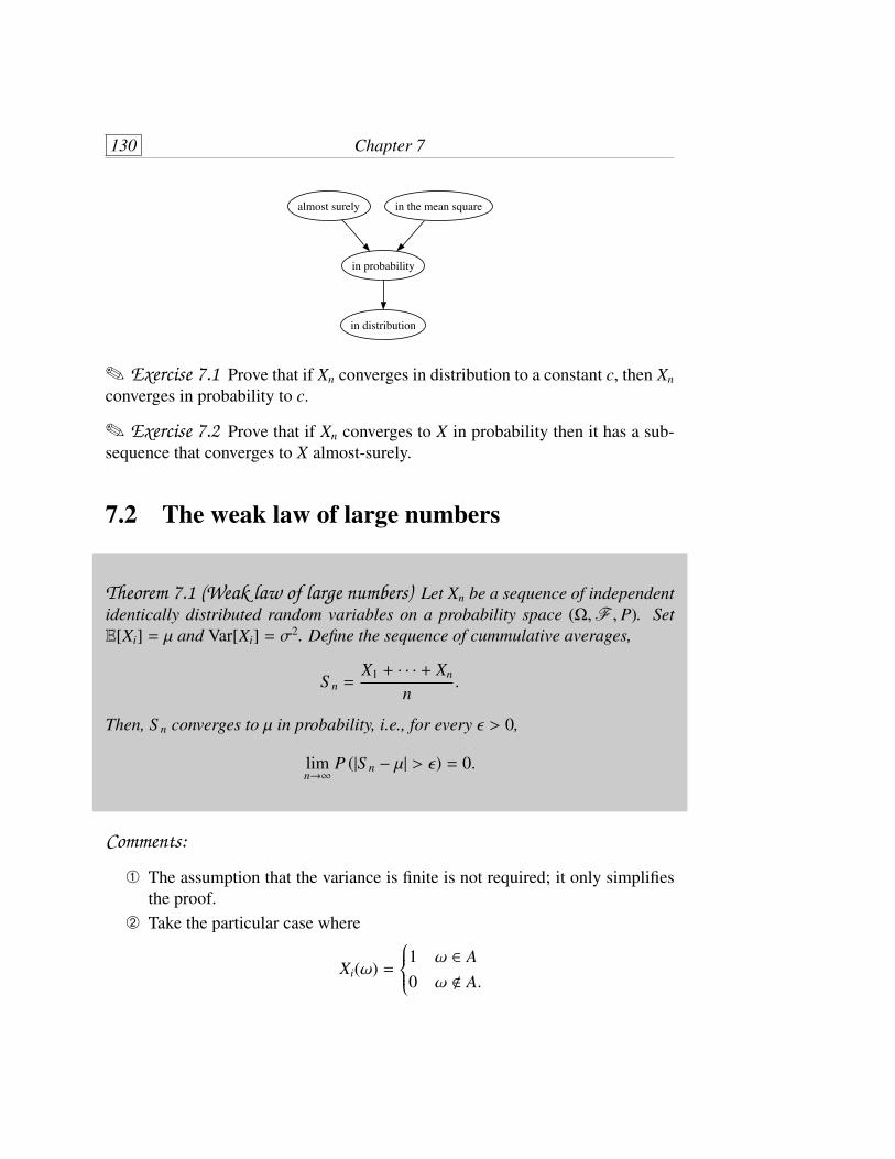
130 Chapter 7
almost surely
in probability
in distribution
in the mean square
+ Exercise 7.1 Prove that if Xn converges in distribution to a constant c, then Xn
converges in probability to c.
+ Exercise 7.2 Prove that if Xn converges to X in probability then it has a sub-sequence that converges to X almost-surely.
7.2 The weak law of large numbers
Theorem 7.1 (Weak law of large numbers) Let Xn be a sequence of independentidentically distributed random variables on a probability space (",F , P). SetE[Xi] = µ and Var[Xi] = $2. Define the sequence of cummulative averages,
S n =X1 + · · · + Xn
n.
Then, S n converges to µ in probability, i.e., for every ( > 0,
limn2*
P (|S n . µ| > () = 0.
Comments:
! The assumption that the variance is finite is not required; it only simplifiesthe proof.
" Take the particular case where
Xi(!) =
@AABAAC
1 ! ! A0 ! ! A.
Limit theorems 131
Then,S n = fraction of times ! ! A.
The weak law of large numbers states that the fraction of times the outcomeis in a given set converges in probability to E[X1], which is the probabilityof this set, P(A).
Proof : This is an immediate consequence of the Chebyshev inequality, for by theadditivity of the expectation and the variance (for independent random variables),
E[S n] = µ and Var[S n] =$2
n.
Then,
P (|S n . µ| > () "Var[S n](2
=$2
n(22 0.
*
Comment: the first proof is due to Jacob Bernoulli (1713), who proved it for theparticular case of binomial variables.
7.3 The central limit theorem
Theorem 7.2 (Central limit theorem) Let (Xn) be a sequence of i.i.d. randomvariables with E[Xi] = 0 and Var[Xi] = 1. Then, the sequence of random variables
S n =X1 + · · · + Xn8
n
converges in distribution to a random variables X 6 N(0, 1). That is,
limn2*
P (S n " a) =182#
L a
.*e.y2/2 dy.
Comments:

132 Chapter 7
! If E[Xi] = µ and Var[Xi] = $2 then the same applies for
S n =X1 + · · · + Xn . nµ
$8
n=
18n
n-
i=1
Xi . µ$.
" The central limit theorem (CLT) is about a running average rescaled by afactor of
8n. If we denote by Yn the running average,
Yn =X1 + · · · + Xn
n,
then the CLT states that
P2Yn "
a8n
36 %(a),
i.e., it provides an estimate of the distribution of Yn at distances O(n.1/2)from its mean. It is a theorem about small deviations from the mean. Thereexist more sophisticated theorems about the distribution of Yn far from themean, part of the so-called theory of large deviations.
# There are many variants of this theorem.
Proof : We will use the following fact, which we won’t prove: if the sequence ofmoment generating functions MXn(t) of a sequence of random variables (Xn) con-verges for every t to the moment generating function MX(t) of a random variableX, then Xn converges to X in distribution. In other words,
MXn(t)2 MX(t) for all t implies that XnD.2 X.
Thus, we need to show that the moment generating functions of the S n’s tendsas n 2 * to exp(t2/2), which is the moment generating function of a standardnormal variable.Recall that the pdf of a sum of two random variables is the convolution of theirpdf, but the moment generating function of their sum is the product of the theirmoment generating function. Inductively,
MX1+X2+...,+Xn(t) =n5
i=1
MXi(t) = [MX1(t)]n,

Limit theorems 133
where we have used the fact that they are i.i.d., Now, if a random variable Y has amoment generating function MY , then
MY/a(t) =L
R
ety fY/a(y) dy,
but since fY/a(y) = a fY(ay) we get that
MY/a(t) = aL
R
ety fY(ay) dy =L
R
eaty/a fY(ay) d(ay) = MY(t/a),
from which we deduce that
MS n(t) =<MX1
2t8n
3=n.
Take the logarithm of both sides, and write the left hand side explicitly,
log MS n(t) = n logL
R
etx/8
n fX1(x) dx.
Taylor expanding the exponential about t = 0 we have,
log MS n(t) = n logL
R
21 +
tx8n+
t2x2
2n+
t3x3
6n3/2 e0x/8
n3
fX1(x) dx
= n log21 + 0 +
t2
2n+ O(n.3/2)
3
= n2
t2
2n+ O(n.3/2)
32 t2
2.
*
Example: Suppose that an experimentalist wants to measure some quantity. Heknows that due to various sources of errors, the result of every single measurementis a random variable, whose mean µ is the correct answer, and the variance ofhis measurement is $2. He therefore performs independent measurements andaverages the results. How many such measurements does he need to perform tobe sure, within 95% certainty, that his estimate does not deviate from the trueresult by $/4?

134 Chapter 7
The question we’re asking is how large should n be in order for the inequality
P
'((((()µ .
$
4" 1
n
n-
k=1
Xk " µ +$
4
*+++++, , 0.95
to hold. This is equivalent to asking what should n be for
P
'((((().8
n4" 18
n
n-
k=1
Xk . µ$
"8
n4
*+++++, , 0.95.
By the central limit theorem the right hand side is, for large n, approximately
282#
L 8n/4
0e.y2/2 dy,
which turns out to be larger than 0.95 for , 62.The problem with this argument that it uses the assumption that “n is large”, butit is not clear what large is. Is n = 62 su!ciently large for this argument to hold?This problem could have been solved without this di!culty but resorting insteadto the Chebyshev inequality:
P
'((((().8
n4" 18
n
n-
k=1
Xk . µ$
"8
n4
*+++++, = 1 . P
'((((()
KKKKKKK18n
n-
k=1
Xk . µ$
KKKKKKK,8
n4
*+++++,
, 1 . 16n,
and the right hand side is larger than 0.95 if
n , 160.05
= 320.
!!!
Example: The number of students X who are going to fail in the exam is a Poissonvariable with mean 100, i.e, X 6 Poi(100). I am going to admit that the exam wastoo hard if more than 120 student fail. What is the probability for it to happen?We know the exact answer,
P (X , 120) = e.100*-
k=120
100k
k!,

Limit theorems 135
which is a quite useless expression. Let’s base our estimate on the central limittheorem as follows: a Poisson variable with mean 100 can be expressed as thesum of one hundred independent variables Xk 6 Poi(1) (the sum of independentPoisson variables is again a Poisson variable), that is X =
4100k=1 Xk. Now,
P (X , 120) = P
'((((()
18100
100-
k=1
Xk . 11, 20
10
*+++++, ,
which by the central limit theorem equals approximately,
P (X , 120) / 182#
L *
2e.y2/2 dy / 0.228.
!!!
Example: Let us examine numerically a particular example. Let Xi 6 Exp (1) beindependent exponential variable and set
S n =18n
n-
i=1
(Xi . 1).
A sum of n independent exponential variables has distribution Gamma (n, 1), i.e.,its pdf is
xn.1e.x
$(n).
The density for this sum shifted by n is
(x + n)n.1e.(x+n)
$(n),
with x > .n and after dividing by8
n,
fS n(x) =8
n(8
nx + n)n.1e.(8
nx+n)
$(n),
with x > .8n. See Figure 7.1 for a visualization of the approach of the distribu-tion of S n toward the standard normal distribution.
!!!

136 Chapter 7
−5 −4 −3 −2 −1 0 1 2 3 4 50
0.1
0.2
0.3
0.4
0.5
0.6
0.7
0.8
0.9
1n=1
−5 −4 −3 −2 −1 0 1 2 3 4 5−0.1
0
0.1
0.2
0.3
0.4
0.5
0.6n=2
−5 −4 −3 −2 −1 0 1 2 3 4 50
0.05
0.1
0.15
0.2
0.25
0.3
0.35
0.4
0.45n=4
−5 −4 −3 −2 −1 0 1 2 3 4 50
0.05
0.1
0.15
0.2
0.25
0.3
0.35
0.4
0.45n=16
Figure 7.1: The approach of a normalized sum of 1, 2, 4 and 16 exponential ran-dom variables to the normal distribution.

Limit theorems 137
7.4 The strong law of large numbers
Our next limit theorem is the strong law of large number, which states that therunning average of a sequence of i.i.d. variables converges to the mean almost-surely (thus strengthening the weak law of large number, which only providesconvergence in probability).
Theorem 7.3 (Strong law of large numbers) Let (Xn) be an i.i.d. sequence ofrandom variables with E[Xi] = 0 and Var[Xi] = $2, then with probability one,
X1 + · · · + Xn
n2 0.
Proof : Set ( > 0, and consider the following sequence of events:
An =
@AABAACmax
1"k"n
KKKKKKK
k-
i=1
Xi
i
KKKKKKK> (
MAANAAO .
From Komogorov’s inequality,
P(An) " 1(2
n-
k=1
$2
k2 .
The (An) are an increasing sequence hence, by the continuity of the probability,
limn2*
P(An) = P>limn2*
An
?= P
'((((()max
1"k
KKKKKKK
k-
i=1
Xi
i
KKKKKKK> (
*+++++, "
C$2
(2,
or equivalently,
P
'((((()max
1"k
KKKKKKK
k-
i=1
Xi
i
KKKKKKK" (*+++++, , 1 . C$2
(2
Since this holds for all ( > 0, taking ( 2 * results in
P
'((((()max
1"k
KKKKKKK
k-
i=1
Xi
i
KKKKKKK< **+++++, = 1.

138 Chapter 7
from which we infer that
P
'((((()*-
i=1
Xi
i< **+++++, = 1,
It is then a consequence of a lemma due to Kronecker that
*-
i=1
Xi
i< * implies lim
n2*1n
n-
k=1
Xk = 0.
*

Limit theorems 139
Lemma 7.1 Let X1 6 N(µ1,$21) and X2 6 N(µ2,$2
2) be independent. Then,
X1 + X2 6 N(µ1 + µ2,$21 + $
22).
Proof : Rather then working with the convolution formula, we use the momentgenerating functions. We have seen that
MX1(t) = exp2$2
1
2t2 + µ1t
3
MX2(t) = exp2$2
2
2t2 + µ2t
3.
Since X1, X2 are independent,
MX1+X2(t) = ESeX1+X2
T= ESeX1TESeX2T,
hence,
MX1+X2(t) = exp2$2
1 + $22
2t2 + (µ1 + µ2)t
3,
from which we identify X1 + X2 as a normal variable with the desired mean andvariance. *
Corollary 7.1 Let Z1,Z2 · · · 6 N(0, 1) be independent. Then for every n ! N,
Z1 + · · · + Zn8n
6 N(0, 1).
Theorem 7.4 Let (Xn) be a sequence of i.i.d. RVs with E[Xi] = 0, Var[Xi] = 1 andE|Xi|3 < *; let S n be defined as above. Let Z1,Z2 · · · 6 N(0, 1) be independent.Then, for every non-negative function +(x), uniformly three-times di!erentiable,and with compact support,
limn2*
KKKKKKE+2
X1 + · · · + Xn8n
3. E+
2Z1 + · · · + Zn8
n
3KKKKKK = 0.
Comments: Suppose we could have taken +(x) = I[a,b](x). Then,
E+(X) = P (a " X " b) ,
140 Chapter 7
and the theorem would imply that
limn2*
KKKKKKP2a " X1 + · · · + Xn8
n" b3. 18
2#
L b
ae.y2/2 dy
KKKKKK = 0.
We are somewhat more restricted by the requirement that + be three time di#eren-tiable, but we can approximate the indicator function by a sequence of smootherfunctions.
Proof : We start with
E+
2X1 + · · · + Xn8
n
3. E+
2Z1 + · · · + Zn8
n
3
= E+
2X1 + · · · + Xn8
n
3. E+
2X1 + · · · + Xn.1 + Zn8
n
3
+ E+
2X1 + · · · + Xn.1 + Zn8
n
3. E+
2X1 + · · · + Xn.2 + Zn.1 + Zn8
n
3
+ . . . ,
so thatKKKKKKE+2
X1 + · · · + Xn8n
3. E+
2Z1 + · · · + Zn8
n
3KKKKKK
"n-
i=1
KKKKKKE+2
X1 + · · · + Xi + Zi+1 + · · · + Zn8n
3. E+
2X1 + · · · + Xi.1 + Zi + · · · + Zn8
n
3.
KKKKKK
Each of the summands can be estimated as follows:KKKKKKE+2
X1 + · · · + Xi + Zi+1 + · · · + Zn8n
3. E+
2X1 + · · · + Xi.1 + Zi + · · · + Zn8
n
3KKKKKK
=
KKKKKKE+2
Xi8n+ un
3. E+
2Zi8
n+ un
3KKKKKK ,
where the un represent all the other terms. We then Taylor expand up to the thirdterm, and replace the expectation by
E[·] = E[E[·|un]].

Limit theorems 141
Using the fact that Xn and Zn have the same first and second moments, and theuniform boundedness of the third derivative of +, we get
KKKKKKE+2
Xi8n+ un
3. E+
2Zi8
n+ un
3KKKKKK "C
n8
n.
Substituting above we conclude thatKKKKKKE+2
X1 + · · · + Xn8n
3. E+
2Z1 + · · · + Zn8
n
3KKKKKK "C8
n2 0.
*

142 Chapter 7

Chapter 8
Markov chains
8.1 Definitions and basic properties
Let S be a set that could be either finite or countable. S is called the state space;elements of S are denoted by indices i, j, . . . , i0, i1, . . . .
Definition 8.1 A Markov chain over S is a sequence of random variables X1, X2, . . . ,satisfying
P(Xn = in|X0 = i0, . . . , Xn.1 = in.1) = P(Xn = in|Xn.1 = in.1).
That is, “the present determines the distribution of the future independently of thepast”. The right hand side is called the transition probability. It depends on n,and on the two states in.1 and in.
Comments:
! A Markov chain is an instance of a stochastic process." We often interpret the index n as time. In a Markov chain time is a discrete
parameter; there are also Markov processes in continuous time (continuous-time Markov processes) and Markov processes over uncountable state spaces(e.g., Brownian motion).
# A Markov chain is called time homogeneous if the transition probability istime-independent, i.e., if
P(Xn = j|Xn.1 = i) = P(Xm = j|Xm.1 = i) ( pi, j.

144 Chapter 8
The matrix P whose entries are pi, j is called the transition matrix (don’t bebothered by infinite matrices). It is the probability to transition from state ito state j in a single step.
The transition matrix P is a stochastic matrix. That is, pi, j , 0 for all i, j ! S and-
j!Spi, j = 1
for all i ! S (note that the sums over columns do not need to be one; a stochasticmatrix having this additional property, i.e., that PT is also stochastic, is calleddoubly stochastic.In addition to the transition matrix, a Markov chain is also characterized by itsinitial distribution, which can be represented by a vector µ with entries
µi = P(X0 = i).
Proposition 8.1 The transition distribution µ and the transition matrix P fullydetermine the distribution of the process (i.e., the distribution of the sequence ofrandom variables).
Proof : A sequence of random variables is fully determined by all its finite-dimensionalmarginal distributions. Using the product formula,
P(A ' B 'C ' · · · ' Z) = P(A|B 'C ' · · · ' Z) P(B|C ' · · · ' Z) · · · P(Z),
along with the Markov property, we have for every n,
P(X0 = i0, . . . , Xn = in) = P(Xn = in|X0 = i0, . . . , Xn.1 = in.1)# P(Xn.1 = in.1|X0 = i0, . . . , Xn.2 = in.2) · · ·# P(X1 = i1|X0 = i0)P(X0 = i0)= µi0 pi0,i1 · · · pin.2,in.1 pin.1,in .
*
Summing the above identity over all values of i1, . . . , in.1 we obtain,
P(Xn = in|X0 = i0) = (Pn)i0,in ( p(n)i0,in .

Markov chains 145
Thus, the n-th power of the transition matrix is the n-step transition matrix; p(n)i, j is
the probability to transition from state i to state j in n steps. It follows at once thatfor all n,m,
p(n+m)i, j =
-
k!Sp(n)
i,k p(m)k, j .
It is also customary to definep(0)
i, j = ,i, j.
Finally, if µ(n) denotes the distribution at time n, i.e.,
µ(n)j = P(Xn = j),
thenµ(n)
j =-
i!SP(Xn = j|X0 = i)P(X0 = i) =
-
i!Sµi pi, j,
namely,µ(n) = µPn,
where we interpret µ as a row vector.
Example: Consider a Markov chain with finite state space. We can represent thestates in S as nodes of a graph. Every two nodes i, j are joined by a directed edgelabeled by the probability to transition from i to j is a single step. If pi, j = 0 thenno edge is drawn. This picture is useful for imagining a simulation of the Markovchain. The initial state is drawn from the distribution µ by “tossing a coin” (well,more precisely by sampling from U (0, 1)). Then, we transition from this state i0
by drawing the next state from the distribution pi0, j, and so on. !!!
Example: Another example is random walk on Zd. For d = 1 we start, say, atthe origin, X0 = 0. Then
Xn+1 =
@AABAAC
Xn . 1 w.p. 1/2Xn + 1 w.p. 1/2.
In higher dimensions we will assume, for technical reasons, that the process movesat each step along all d axes. Thus, for d = 2, we have
Xn+1 = Xn + (±1,±1),
each four transitions having equal probability. !!!

146 Chapter 8
8.2 Transience and recurrence
We define now the following probability:
f (n)i, j = P(Xn = j, Xn.1 " j, . . . , X1 " j|X0 = i).
It is the probability that the process arrives at state j at time n for the first time,given that it started in state i. Note that the events “the process arrived to state j forthe first time at time n”, with n varying, are mutually disjoint, and their countableunion is the event that the process arrived to state j eventually. That is,
fi, j =
*-
n=1
f (n)i, j
is the probability that a process that started in state i will eventually get to state j.In particular, f j, j is the probability that a process starting in state j will eventuallyreturn to its stating point.
Definition 8.2 A state j ! S is called persistent if a process stating in this statehas probability one to eventually return to it, i.e., if f j, j = 1. Otherwise, it is calledtransient.
Suppose that the process started in state i. The probability that it visited state j forthe first time at time n1, for the second time at time n2, and so on, until the k-thtime at time nk is
f (n1)i, j f (n2.n1)
j, j · · · f (nk.nk.1)j, j .
The probability that there were eventually k visits in j is obtained by summingover all possible values of the n1, . . . , nk, giving,
P(at least k visits in j|X0 = i) = fi, j f kj, j.
Letting k 2 * we get that the probability of having infinitely many visits in statej is
P(Xn = j i.o.|X0 = i) =
@AABAAC
fi, j f j, j = 10 f j, j < 1.
.
Taking j = i, we get that the process returns to its stating point infinitely manytimes with a probability that is either zero or one (yet another zero-one law),
P(Xn = i i.o.|X0 = i) =
@AABAAC
1 fi,i = 10 fi,i < 1.
.
Markov chains 147
This means that
One guaranteed return is equivalent to infinitely many guaranteed returns.
The question is how to identify whether a state is recurrent or transient given theMarkov transition matrix. This is settled by the following theorem:
Theorem 8.1 The following characterization of persistence are equivalent:
fi,i = 1 C P(Xn = i i.o.|X0 = i) = 1 C*-
n=1
p(n)i,i = *.
Similarly for transience,
fi,i < 1 C P(Xn = i i.o.|X0 = i) = 0 C*-
n=1
p(n)i,i < *.
Proof : It is enough to show the correctness for transience. We have already seenthat transience is equivalent to the probability of infinitely many returns beingzero. By the first Borel-Cantelli lemma the finiteness of the series implies as wellthat the probability of infinitely many returns is zero. It remains to show thattransience implies the finiteness of the series. We have
p(n)i, j =
n.1-
s=0
P(Xn = j, Xn.s = j, Xn.s.1 " j, . . . , X1 " j|X0 = i)
=
n.1-
s=0
P(Xn = j|Xn.s = j)P(Xn.s = j, Xn.s.1 " j, . . . , X1 " j|X0 = i)
=
n.1-
s=0
p(s)j, j f (n.s)
i, j .
This decomposition is called a first passage time decomposition. We then seti = j and sum over n,
m-
n=1
p(n)i,i =
m-
n=1
n.1-
s=0
p(s)i,i f (n.s)
i,i =
m.1-
s=0
m-
n=s+1
p(s)i,i f (n.s)
i,i =
m.1-
s=0
p(s)i,i
m.s-
n=1
f (n)i,i " fi,i
m-
s=0
p(s)i,i

148 Chapter 8
This means thatm-
n=1
p(n)i,i " fi,i + fi,i
m-
s=1
p(s)i,i ,
where we have used the fact that fi,i(0) = 1, or,
(1 . fi,i)m-
n=1
p(n)i,i " fi,i.
If fi,i < 1 then we have a uniform bound on the series. *
Example: Random walks in Zd. Since
p(n)0,0 6
1nd/2 ,
then the origin (and any other state by symmetry) is recurrent in dimensions oneand two and transient in dimensions higher than two. !!!
Definition 8.3 A Markov chain is called irreducible if, loosely speaking, it ispossible to reach every state from every other state. More precisely, if for everyi, j ! S there exists an n for which
p(n)i, j > 0.
Theorem 8.2 In an irreducible Markov chain one of the following holds:
! All the states are transient, and for all i, j,
P0% j!S {Xn = j i.o.} |X0 = i
1= 0,
and *-
n=1
p(n)i, j < *.
" All the states are persistent, and for all i, j,
P0' j!S {Xn = j i.o.} |X0 = i
1= 1,
and *-
n=1
p(n)i, j = *.

Markov chains 149
Comment: This implies that provided that one state is persistent, irrespectively ofthe initial state, the chain is guaranteed to visit every state infinitely many times.This is highly non-trivial.
Proof : Let i, j ! S be given. Since the chain is irreducible, then there exist m, rsuch that p(m)
i, j > 0 and p(r)j,i > 0. For all n,
p(m+n+r)i,i " p(m)
i, j p(n)j, j p(r)
j,i .
Summing over n, it follows that if j is transient so is i. That is, transience (andhence persistence) is a property of all states.We saw that
p(Xn = j i.o.|X0 = i) =
@AABAAC
0 f j, j < 1fi, j f j, j = 1.
Thus, if the chain is transient, then this is zero for all i, j. By Boole’s inequalitya countable union of the event of zero probability has zero probability. Finally,using again the first passage trick,
p(n)i, j =
n-
s=0
f (s)i, j p(n.s)
j, j ,
hence,
*-
n=1
p(n)i, j =
*-
n=1
n-
s=0
f (s)i, j p(n.s)
j, j =
*-
s=0
f (s)i, j
*-
n=s
p(n.s)j, j = fi, j
*-
n=0
p(n)j, j < *.
Conversely, suppose the chain is persistent, i.e., f j, j = 1 for all j. We then knowthat
p(Xn = j i.o.|X0 = i) = fi, j.
For every m,
p(m)j,i = P({Xm = i} ' {Xn = j i.o.} |X0 = j)
"-
n>m
P(Xm = i, Xm+1 " j, . . . , Xn = j|X0 = j)
=-
n>m
p(m)j,i f (n.m)
i, j = fi, j p(m)j,i .

150 Chapter 8
Since there exists an m for which the left-hand side is positive, it follows thatfi, j = 1. Then, the countable intersection of certain events has probability one.Finally, if
*-
n=1
p(n)i, j < *,
then by the first Borel-Cantelli lemma
p(Xn = j i.o.|X0 = i) = 0,
which is a contradiction. *
Corollary 8.1 A finite irreducible Markov chain is persistent.
Proof : Since for all i, -
j!Sp(n)
i, j = 1,
then1|S |-
j!S
*-
n=1
p(n)i, j = *.
It follows that4*
n=1 p(n)i, j = * for all i, j. *
8.3 Long-time behavior
We now turn to discuss the long time behavior of Markov chains. Recall that ifµ(n) is the distribution at time n then
µ(n)i =
-
j!Sµ(n.1)
j p j,i,
and inductively,µ(n)
i =-
j!Sµ(0)
j (Pn) j,i.
The question is whether the distribution has a limit as n2 * and what it is. Notefirst that if a limit µ = ! exists, then
! = !P,

Markov chains 151
i.e., it is a stationary distribution of the Markov chain; it is also a left eigenvectorof P with eigenvalue 1.
Example: To get some idea on what is going on, consider a two-state Markovchain with transition matrix
P =21 . p p
q 1 . q
3,
with 0 < p, q < 1. For such a simple matrix we can easily calculate its n-th power.The eigenvalues satisfy
<1 . p . ' p
q 1 . q . '
== 0,
i.e.,'2 . (2 . p . q)' + (1 . p . q) = 0.
Setting 1 . p . q = & we have
'1,2 =12
0(1 + &) ±
J(1 + &)2 . 4&
1= 1,&.
The eigenvector that corresponds to ' = 1 is (1, 1)T . The eigenvector that corre-sponds to ' = & satisfies 2
q pq p
3 2xy
3= 0,
i.e., (p,.q)T . Normalizing we have
S =21/8
2 p/J
p2 + q2
1/8
2 .q/J
p2 + q2
3and S .1 = .
82J
p2 + q2
p + q
2.q/J
p2 + q2 .p/J
p2 + q2
.1/8
2 1/8
2
3.
SinceP = S'S .1,
it follows that Pn = S'nS .1 and as n2 *
limn2*
Pn = S21 00 0
3S .1 =
1p + q
2q pq p
3.
For every µ(0) we get
limn2*µ(n) =
(q, p)p + q
.
Thus, the distribution converges to the (unique) stationary distribution irrespec-tively of the initial distribution. !!!