Lecture 7 Rolling Constraints 

The most common, and most important nonholonomic constraints 

They cannot be wri5en in terms of the variables alone  you must include some deriva9ves 

The resul9ng differen9al is not integrable 

1 

The major assump9on/simplifica9on is point contact 

This is true of a rigid hoop on a rigid surface 

or a rigid sphere on a rigid surface 

2 

I will also generally assume that the surface is horizontal  so that gravity is normal to the surface 

3 

rigid hoop on a rigid surface 

4 

rigid sphere on a rigid surface 

5 

It’s not a bad approxima9on for a well‐inflated bicycle or motorcycle 9re  on hard pavement 

It’s not so good for an automobile 9re, which has a pre5y big patch on the ground 

Cylindrical wheels, like those on grocery carts and children’s toys  must slip over parts of their surfaces when turning 

We aren’t going to care about any of this  We’re going to suppose that all the wheels we consider have point contact 

6 

Two fundamental ideas: 

The speed of a point rota9ng about a fixed point is 

€

v =ω × r

The contact point between a wheel and the ground is not moving 

7 

For a sphere of radius a r = ak 

€

v = aω ×k = aωy

−ωx

0

This is iner9al , so we have  

€

v = aωy

−ωx

0

= a

˙ θ sinφ − ˙ ψ cosφ sinθ− ˙ θ cosφ − ˙ ψ sinφ sinθ

0

8 

€

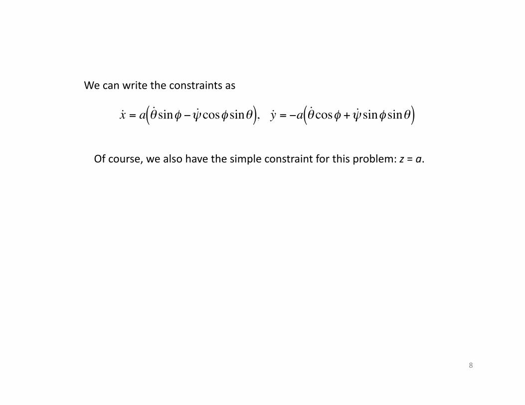
˙ x = a ˙ θ sinφ − ˙ ψ cosφ sinθ( ), ˙ y = −a ˙ θ cosφ + ˙ ψ sinφ sinθ( )

We can write the constraints as 

Of course, we also have the simple constraint for this problem: z = a. 

9 

An erect wheel has the same r 

If we choose to let the axle be the K body coordinate  then θ = ±π/2, fixed, and the constraint becomes 

€

v = aωy

−ωx

0

= a

˙ θ sinφ − ˙ ψ cosφ sinθ− ˙ θ cosφ − ˙ ψ sinφ sinθ

0

€

v = a

˙ ψ cosφ− ˙ ψ sinφ

0

⇒ ˙ x = −a ˙ ψ cosφ, ˙ y = −a ˙ ψ sinφ

The general wheel is fancier; I’ll get to that shortly 

BUT FIRST 

10 

How do we impose these? 

The classical method is through Lagrange mul9pliers,  and that’s what we’ll do today 

(There’s an alternate method that we will see later in the semester) 

To get at this we need to go back to first principles  and it helps to note that we can write the constraints in matrix form 

11 

€

˙ x = a ˙ θ sinφ + ˙ ψ cosφ sinθ( ), ˙ y = −a ˙ θ cosφ + ˙ ψ sinφ sinθ( )

€

q =

xyzφ

θ

ψ

€

˙ q 1 − a ˙ q 5 sinq4 + ˙ q 6 cosq4 sinq5( ) = 0 = ˙ q 2 + a ˙ q 5 cosq4 + ˙ q 6 sinq4 sinq5( )

12 

€

1 0 0 0 −asinq4 −acosq4 sinq5

0 1 0 0 acosq4 asinq4 sinq5

˙ q 1

˙ q 2

˙ q 3

˙ q 4

˙ q 5

˙ q 6

= 0

€

˙ q 1 − a ˙ q 5 sinq4 + ˙ q 6 cosq4 sinq5( ) = 0 = ˙ q 2 + a ˙ q 5 cosq4 + ˙ q 6 sinq4 sinq5( )

€

C ˙ q = 0⇔C ji ˙ q j

13 

We can view the 9me deriva9ve of q as a surrogate for δq 

€

C jiδq j = 0

€

dI η( )dη

= 0 =∂L *∂qk −

ddt

∂L *∂ ˙ q k

∂qk

∂ηdt

t1

t2∫ =∂L *∂qk −

ddt

∂L *∂ ˙ q k

δqkdt

t1

t2∫

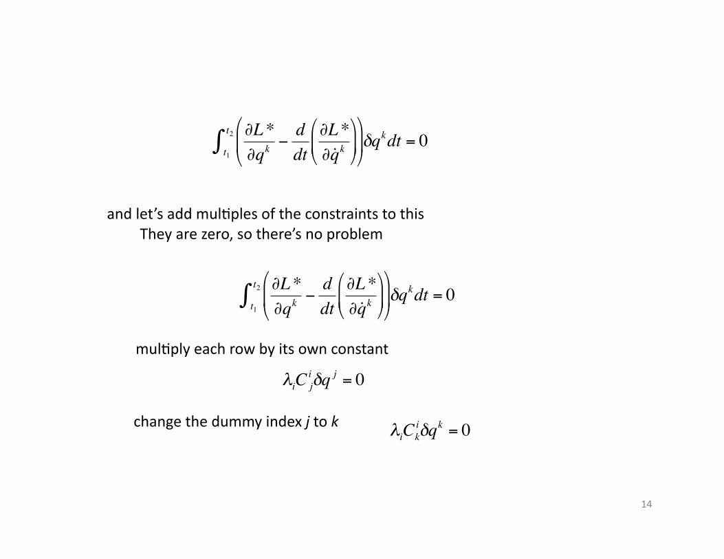
Now let’s go back to lecture two and the ac9on integral it is sta9onary if 

Consider the final version 

14 

€

∂L *∂qk −

ddt

∂L *∂ ˙ q k

δqkdt

t1

t2∫ = 0

and let’s add mul9ples of the constraints to this  They are zero, so there’s no problem 

€

∂L *∂qk −

ddt

∂L *∂ ˙ q k

δqkdt

t1

t2∫ = 0

€

λiC jiδq j = 0

€

λiCkiδqk = 0

mul9ply each row by its own constant 

change the dummy index j to k 

15 

€

∂L *∂qk −

ddt

∂L *∂ ˙ q k

+ λiCk

i

δqkdt

t1

t2∫ = 0

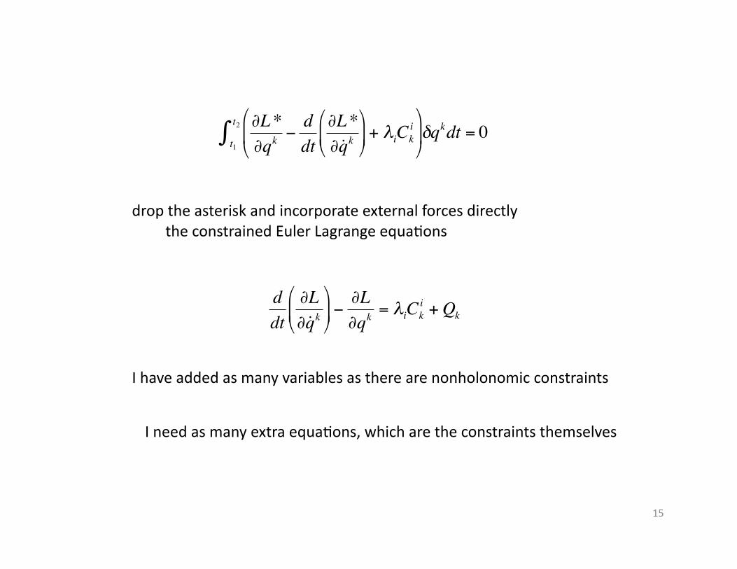
drop the asterisk and incorporate external forces directly  the constrained Euler Lagrange equa9ons 

€

ddt

∂L∂ ˙ q k

−

∂L∂qk = λiCk

i + Qk

I have added as many variables as there are nonholonomic constraints 

I need as many extra equa9ons, which are the constraints themselves 

16 

€

ddt

∂L∂ ˙ q k

−

∂L∂qk = λiCk

i + Qk

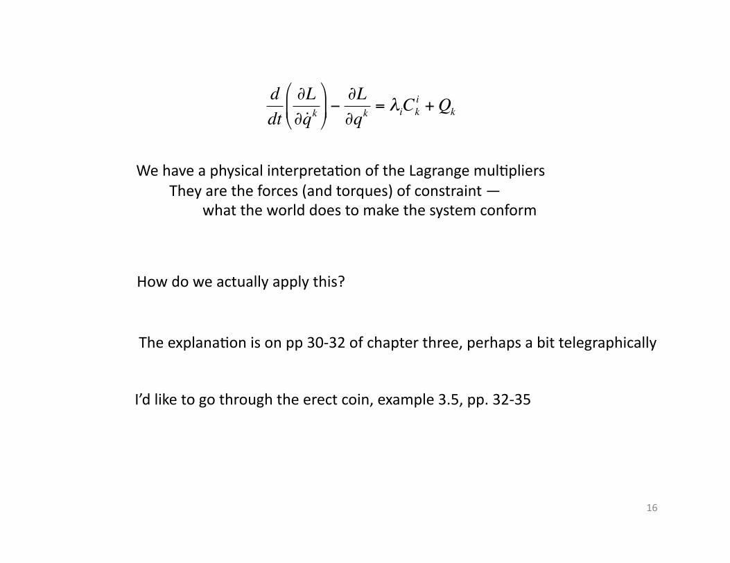
We have a physical interpreta9on of the Lagrange mul9pliers  They are the forces (and torques) of constraint —    what the world does to make the system conform 

How do we actually apply this? 

The explana9on is on pp 30‐32 of chapter three, perhaps a bit telegraphically 

I’d like to go through the erect coin, example 3.5, pp. 32‐35 

17 

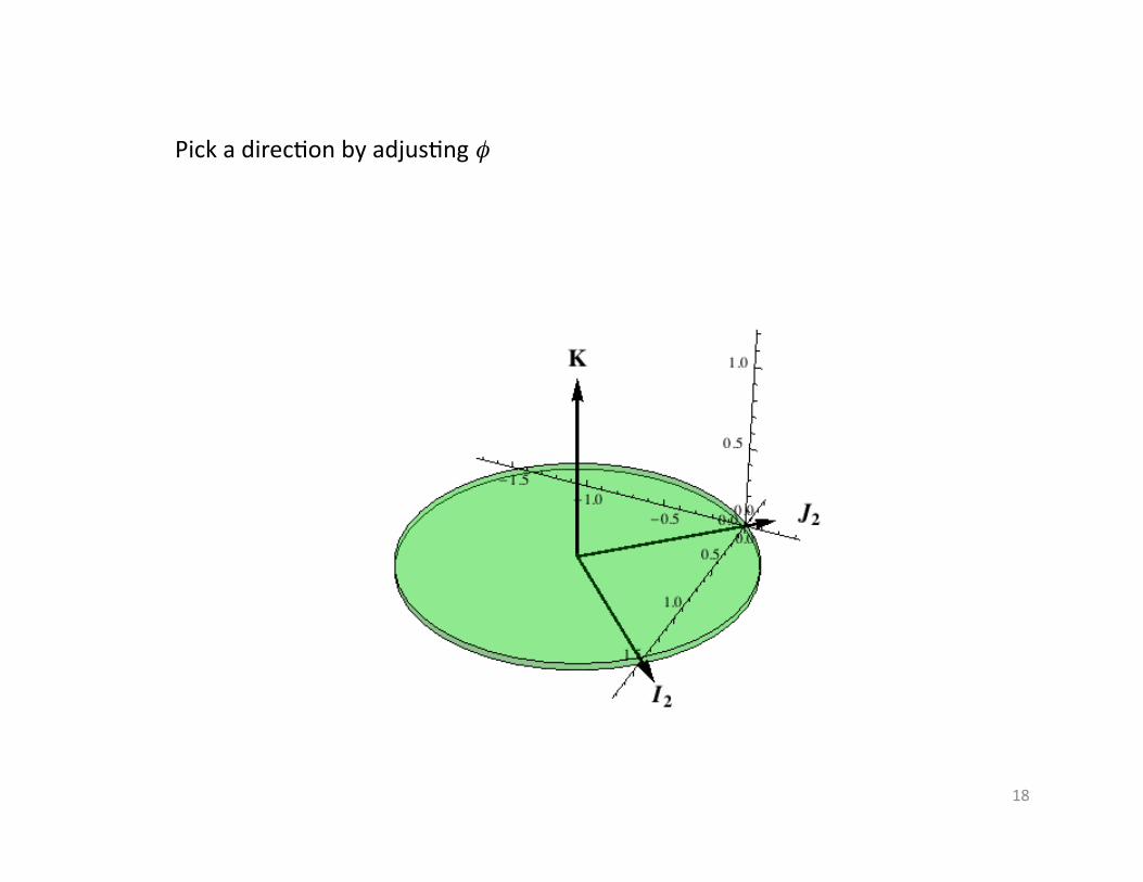
First let’s see how we can set up a wheel 

I like the axle to be the K axis; let’s see how we can erect the wheel 

Star9ng with all Euler angles equal to zero 

18 

Pick a direc9on by adjus9ng φ

19 

erect the wheel with θ = ‐π/2  (the text example uses + π/2) 

20 

€

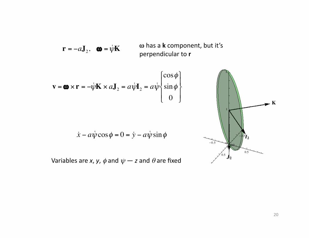
r = −aJ2, ω = ˙ ψ K

€

v =ω × r = − ˙ ψ K × aJ2 = a ˙ ψ I2 = a ˙ ψ

cosφsinφ

0

€

˙ x − a ˙ ψ cosφ = 0 = ˙ y − a ˙ ψ sinφ

Variables are x, y, φ and ψ — z and θ are fixed 

ω has a k component, but it’s perpendicular to r 

21 

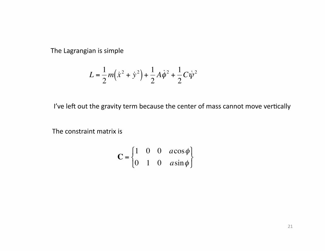
The Lagrangian is simple 

€

L =12

m ˙ x 2 + ˙ y 2( ) +12

A ˙ φ 2 +12

C ˙ ψ 2

I’ve lek out the gravity term because the center of mass cannot move ver9cally 

The constraint matrix is 

€

C =1 0 0 acosφ0 1 0 asinφ

22 

The product 

€

λC = λ1 λ2{ }1 0 0 acosφ0 1 0 asinφ

= λ1 λ2 0 a λ1 cosφ + λ2 sinφ( ){ }

The Lagrange equa9ons are then 

€

m˙ ̇ x = λ1, m˙ ̇ y = λ2, ˙ ̇ φ = 0, ˙ ̇ ψ =aC

λ1 cosφ + λ2 sinφ( )

and the constraints are 

€

˙ x − a ˙ ψ cosφ = 0 = ˙ y − a ˙ ψ sinφ

23 

So I have six equa9ons in six unknowns: the variables and the mul9pliers 

Solve the first two dynamical equa9ons for the mul9pliers 

€

λ1 = m˙ ̇ x , λ2 = m˙ ̇ y

The remaining dynamical equa9ons become 

€

˙ ̇ φ = 0, ˙ ̇ ψ =amC

˙ ̇ x cosφ + ˙ ̇ y sinφ( )

and I can use the constraints to eliminate the accelera9on terms 

24 

€

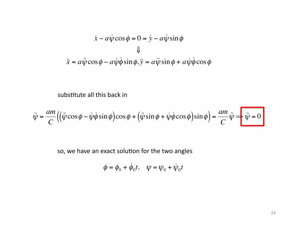
˙ x − a ˙ ψ cosφ = 0 = ˙ y − a ˙ ψ sinφ⇓

˙ ̇ x = a ˙ ̇ ψ cosφ − a ˙ ψ ̇ φ sinφ, ˙ ̇ y = a ˙ ̇ ψ sinφ + a ˙ ψ ̇ φ cosφ

subs9tute all this back in 

€

˙ ̇ ψ =amC

˙ ̇ ψ cosφ − ˙ ψ ̇ φ sinφ( )cosφ + ˙ ̇ ψ sinφ + ˙ ψ ̇ φ cosφ( )sinφ( ) =amC

˙ ̇ ψ ⇒ ˙ ̇ ψ = 0

€

φ = φ0 + ˙ φ 0t, ψ =ψ0 + ˙ ψ 0t

so, we have an exact solu9on for the two angles 

25 

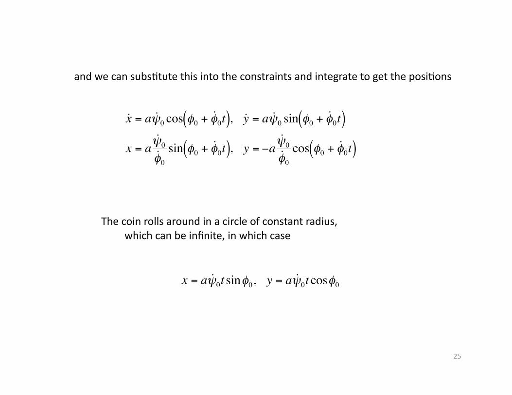
and we can subs9tute this into the constraints and integrate to get the posi9ons 

€

˙ x = a ˙ ψ 0 cos φ0 + ˙ φ 0t( ), ˙ y = a ˙ ψ 0 sin φ0 + ˙ φ 0t( )

x = a˙ ψ 0˙ φ 0

sin φ0 + ˙ φ 0t( ), y = −a˙ ψ 0˙ φ 0

cos φ0 + ˙ φ 0t( )

The coin rolls around in a circle of constant radius,  which can be infinite, in which case 

€

x = a ˙ ψ 0t sinφ0, y = a ˙ ψ 0t cosφ0

26 

Suppose we consider a general rolling coin,  one not held ver9cal 

The book doesn’t deal with this un9l chapter five,  but we can certainly set it up here.    It’s a hard problem and does not have a closed form solu9on 

27 

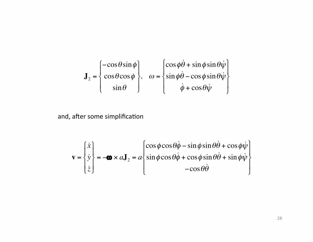
This has the same body system as before  but the angle θ can vary    (it’s equal to ‐0.65π here) 

r remains equal to –aJ2  but we need the whole ω  

28 

€

J2 =

−cosθ sinφcosθ cosφ

sinθ

, ω =

cosφ ˙ θ + sinφ sinθ ˙ ψ

sinφ ˙ θ − cosφ sinθ ˙ ψ ˙ φ + cosθ ˙ ψ

and, aker some simplifica9on 

€

v =

˙ x ˙ y ˙ z

= −ω × aJ2 = acosφ cosθ ˙ φ − sinφ sinθ ˙ θ + cosφ ˙ ψ

sinφ cosθ ˙ φ + cosφ sinθ ˙ θ + sinφ ˙ ψ

−cosθ ˙ θ

29 

€

˙ x − a cosφ cosθ ˙ φ − sinφ sinθ ˙ θ + cosφ ˙ ψ ( ) = 0

˙ y − a sinφ cosθ ˙ φ + cosφ sinθ ˙ θ + sinφ ˙ ψ ( ) = 0

˙ z + acosθ ˙ θ = 0

The last one is actually integrable, but I won’t do that 

We have a constraint matrix that appears to disagree   with the one on p. 15 of chapter five. 

The difference stems from the assump9on in the book that θ ≥ 0  whereas in the picture here, θ ≤ 0. 

Choose the one that fits your idea of the ini9al condi9ons. 

30 

I will use the book’s picture, and I will go to Mathema9ca  to analyze this system