Lecture 5. Fractal Properties of Gaussian Random Fields

Lecture 5. Fractal Properties ofGaussian Random Fields

Yimin Xiao

Michigan State UniversityCBMS Conference, University of Alabama in

Huntsville

August 2–6, 2021

Yimin Xiao (Michigan State University) Lecture 5. Fractal Properties of Gaussian Random Fields August 2–6, 2021 1 / 44

Outline

An introduction to fractal geometryHausdorff measure and Hausdorff dimensionPacking measure and packing dimension

Exact Hausdorff measure functions for the range offBm

Exact packing measure functions for the range of fBm

Chung’s LIL for fBm and its exceptional sets


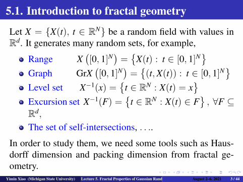
5.1. Introduction to fractal geometry

Let X = X(t), t ∈ RN be a random field with values inRd. It generates many random sets, for example,

Range X([0, 1]N

)=

X(t) : t ∈ [0, 1]N

Graph GrX([0, 1]N

)=

(t,X(t)) : t ∈ [0, 1]N

Level set X−1(x) =

t ∈ RN : X(t) = x

Excursion set X−1(F) =

t ∈ RN : X(t) ∈ F, ∀F ⊆

Rd,

The set of self-intersections, . . ..

In order to study them, we need some tools such as Haus-dorff dimension and packing dimension from fractal ge-ometry.


5.1 Definitions of Hausdorff measure anddimension

Let Φ be the class of functions ϕ : (0, δ) → (0,∞) whichare right continuous, monotone increasing with ϕ(0+) = 0and such that there exists a finite constant K > 0 such that

ϕ(2s)ϕ(s)

≤ K for 0 < s <12δ.

A function ϕ in Φ is often called a measure function orgauge function.For example, ϕ(s) = sα (α > 0) andϕ(s) = sα log log(1/s)are measure functions.


Given ϕ ∈ Φ, the ϕ-Hausdorff measure of E ⊆ Rd isdefined by

ϕ-m(E) = limε→0

inf∑

i

ϕ(2ri) : E ⊆∞⋃

i=1

B(xi, ri), ri < ε

, (1)

where B(x, r) denotes the open ball of radius r centered atx. The sequence of balls satisfying the two conditions onthe right-hand side of (1) is called an ε-covering of E.

It can be shown that ϕ-m is a metric outer measure and allBorel sets in Rd is ϕ-m measurable.

A function ϕ ∈ Φ is called an exact Hausdorff measurefunction for E if 0 < ϕ-m(E) <∞.


If ϕ(s) = sα, we write ϕ-m(E) asHα(E).The Hausdorff dimension of E is defined by

dimHE = infα > 0 : Hα(E) = 0

= sup

α > 0 : Hα(E) =∞,

Convention: sup∅ := 0.

Hausdorff dimension has the following properties:

1 E ⊆ F ⊆ Rd ⇒ dimHE ≤ dimHF ≤ d.2 (σ-stability):

dimH

( ∞⋃j=1

Ej

)= sup

j≥1dimHEj.


An upper density theorem

For any Borel measure µ on Rd and ϕ ∈ Φ, the upper ϕ-density of µ at x ∈ Rd is defined as

Dϕ

µ(x) = lim supr→0

µ(B(x, r))

ϕ(2r).

Lemma 5.1 [Rogers and Taylor, 1961]Given ϕ ∈ Φ, ∃K > 0 such that for any Borel measureµ on Rd with 0 < ‖µ‖=µ(Rd) < ∞ and every Borel setE ⊆ Rd, we have

K−1µ(E) infx∈E

Dϕ

µ(x)−1 ≤ ϕ-m(E) ≤ K‖µ‖ sup

x∈E

Dϕ

µ(x)−1

.


5.2 Packing measure and packing dimensionThey were introduced by Tricot (1982), Taylor and Tricot(1985). For any ϕ ∈ Φ and E ⊆ Rd, define

ϕ-P(E) = limε→0

sup∑

i

ϕ(2ri) : B(xi, ri) is an ε-packing.

Here ε-packing means that the balls are disjoint, xi ∈ Eand ri ≤ ε.The packing measure ϕ-p of E is defined as:

ϕ-p(E) = inf∑

n

ϕ-P(En) : E ⊆⋃

n

En

.

A function ϕ ∈ Φ is called an exact packing measure func-tion for E for E if 0 < ϕ-p(E) <∞.


If ϕ(s) = sα, we write ϕ-p(E) as Pα(E). The packingdimension of E is defined as:

dimPE = infα > 0 : Pα(E) = 0.

Comparison between dimH and dimP:For any ϕ ∈ Φ and E ⊆ Rd,

ϕ-m(E) ≤ ϕ-p(E), dimHE ≤ dimPE.


A lower density theoremFor any Borel measure µ on Rd and ϕ ∈ Φ, the lower ϕ-density of µ at x ∈ Rd is defined as

Dϕµ(x) = lim inf

r→0

µ(B(x, r))

ϕ(2r).

Lemma 5.2 [Taylor and Tricot, 1985]Given ϕ ∈ Φ, ∃K > 0 such that for any Borel measureµ on Rd with 0 < ‖µ‖=µ(Rd) < ∞ and every Borel setE ⊆ Rd, we have

K−1µ(E) infx∈E

Dϕµ(x)

−1 ≤ ϕ-p(E) ≤ K‖µ‖ supx∈E

Dϕµ(x)

−1.


Example: Cantor’s set

Let C denote the standard ternary Cantor set in [0 , 1]. Atthe nth stage of its construction, C is covered by 2n inter-vals of length/diameter 3−n each.It can be proved that

dimHC = dimPC = log3 2.

By using the upper and lower density theorems, one canprove that

0 < Hlog3 2(C) ≤ Plog3 2(C) <∞.


Example: the range of Brownian motionLet B([0, 1]) be the image of Brownian motion in Rd. Levy(1948) and Taylor (1953) proved that

dimHB([0, 1]) = mind, 2 a.s.

Ciesielski and Taylor (1962), Ray and Taylor (1964) provedthat

0 < ϕd-m(B([0, 1])

)<∞ a.s.,

where

ϕ1(r) = r,

ϕ2(r) = r2 log(1/r) log log log(1/r),

ϕd(r) = r2 log log(1/r), if d ≥ 3.


Taylor and Tricot (1985) proved that

dimPB([0, 1]) = mind, 2

and, if d ≥ 3, then

0 < ψ-p(B([0, 1])

)<∞ a.s.,

where ψ(r) = r2/ log log(1/r).

LeGall and Taylor (1986) proved that, if d = 2, then forany measure function ϕ, either ϕ-p

(B([0, 1])

)= 0 or∞.

Question: How to extend the above results to Gaussianrandom fields?


5.3. Exact Hausdorff and packing measurefunctions for fractional Brownian motionFor H ∈ (0, 1), the fBm BH = BH(t), t ∈ RN with in-dex H is a centered (N, d)-Gaussian field whose covariancefunction is

E[BH

i (s)BHj (t)

]=

12δij(|s|2H + |t|2H − |s− t|2H) ,

where δij = 1 if i = j and 0 otherwise.When N = 1 and H = 1/2, BH is Brownian motion.BH is H-self-similar and has stationary increments.

Kahane (1985) proved that

dimHBH([0, 1]N) = min

d,NH

a.s.


5.3.1 Exact Hausdorff measure functions forBH([0, 1]N) and GrBH([0, 1]N)

Theorem 5.1 [Talagrand (1995, 1998)]Let BH = BH(t), t ∈ RN be a fBm with values in Rd.(i). If N < Hd, then

K−1 ≤ ϕ1-m(BH([0, 1]N)

)≤ K, a.s.

where ϕ1(r) = rNH log log(1/r).

(ii). If N = Hd, then ϕ2-m(BH([0, 1]N)

)is σ-finite, where

ϕ2(r) = rd log(1/r) log log log(1/r).


Theorem 5.2 [X. (1997)]Let BH = BH(t), t ∈ RN be a fBm with values in Rd.(i). If N < Hd, then

K−1 ≤ ϕ1-m(GrBH([0, 1]N)

)≤ K, a.s.

where ϕ1(r) = rNH log log(1/r).

(ii). If N > Hd, then

K−1 ≤ ϕ3-m(GrBH([0, 1]N)

)≤ K, a.s.,

whereϕ2(r) = rN+(1−H)d( log log(1/r)

)Hd/N.


5.3.2. Exact packing measure function forBH([0, 1]N)

Theorem 5.3 (Xiao, 1996, 2003)Let BH = BH(t), t ∈ RN be a fBm with values in Rd. IfN < Hd, then there exists a finite constant K ≥ 1 such that

K−1 ≤ ϕ4-p(BH([0, 1]N)) ≤ K, a.s.

where ϕ4(r) = rNH(

log log(1/r))−N/(2H).


For proving Theorem 5.3, one needs to study the liminfbehavior of the sojourn measure

T(r) =

∫RN

1|BH(t)|≤rdt.

A key ingredient is the following small ball probability es-timate for T(1).

Lemma 5.4 [Xiao, 1996, 2003]Assume that N < Hd. Then there exists a positive andfinite constant K ≥ 1, depending only on H, N and d suchthat for any 0 < ε < 1,

exp(− Kε2H/N

)≤ PT(1) < ε ≤ exp

(− 1

Kε2H/N

).


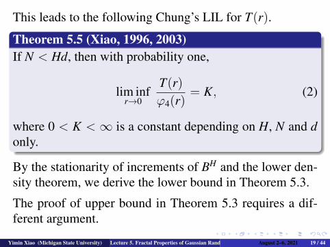
This leads to the following Chung’s LIL for T(r).

Theorem 5.5 (Xiao, 1996, 2003)If N < Hd, then with probability one,

lim infr→0

T(r)

ϕ4(r)= K, (2)

where 0 < K <∞ is a constant depending on H, N and donly.

By the stationarity of increments of BH and the lower den-sity theorem, we derive the lower bound in Theorem 5.3.

The proof of upper bound in Theorem 5.3 requires a dif-ferent argument.


5.4 Exact Hausdorff measure function for theranges of Gaussian random fieldsLet X = X(t), t ∈ RN be a Gaussian field in Rd:

X(t) =(X1(t), . . . ,Xd(t)

), t ∈ RN , (3)

where X1, . . . ,Xd are independent copies of a centered Gaus-sian field X0. We assume that X0 satisfies the followingconditions from Lecture 3.Assumption (A1)Consider a compact interval T ⊂ RN . There exists a Gaus-sian random field v(A, t) : A ∈ B(R+), t ∈ T such that(a) For all t ∈ T , A 7→ v(A, t) is a real-valued Gaussiannoise, v(R+, t) = X0(t), and v(A, ·) and v(B, ·) are inde-pendent whenever A and B are disjoint.


Assumption (A1) (continued)(b) There are constants a0 ≥ 0 and γj > 0, j = 1, . . . ,Nsuch that for all a0 ≤ a ≤ b ≤ ∞ and s = (s1, . . . , sN), t =(t1, . . . , tN) ∈ T ,∥∥v([a, b), s)− X0(s)− v([a, b), t) + X0(t)

∥∥L2

≤ C( N∑

j=1

aγj|sj − tj|+ b−1),

(4)

where ‖Y‖L2 =[E(Y2)

]1/2 for a random variable Y and

∥∥v([0, a0), s)− v([0, a0), t)∥∥

L2 ≤ CN∑

j=1

|sj − tj|. (5)


Condition (A4′) [strong local nondeterminism]There exists a constant c > 0 such that ∀ n ≥ 1 andu, t1, . . . , tn ∈ T ,

Var(X0(u)

∣∣X0(t1), . . . ,X0(tn))≥ c min

1≤k≤nρ(u, tk)2, (6)

where ρ(s, t) is the metric on RN defined by

ρ(s, t) =N∑

j=1

|sj − tj|Hj ,

and where Hj = (γj + 1)−1 (j = 1, . . . ,N).

These conditions are weaker than those in Luan and X.(2012).


Theorem 5.6Let X = X(t), t ∈ RN be a centered Gaussian field withvalues in Rd such that X0 satisfies (A1) and (A4′).

(i). If Q =N∑

j=1H−1

j < d, then

K−1 ≤ ϕ5-m(X([0, 1]N)

)≤ K, a.s., (7)

where ϕ5(r) = rQ log log(1/r).(ii). If Q > d, then X([0, 1]N) has positive d-dimensionalLebesgue measure a.s.

The problem to determine the exact Hausdorff measurefunction for X([0, 1]N) in the “critical case” Q = d is open.


Proof of Theorem 5.6

The lower bound in (7) is proved by using the upper densitytheorem in Lemma 5.1. A natural measure on X([0, 1]N) isthe sojourn measure

µ(B) = λN

t ∈ [0, 1]N : X(t) ∈ B, ∀B ∈ B(Rd),

where λN denotes the Lebesgue measure on RN .For any 0 < r < 1 and t0 ∈ [0, 1]N := I, we consider

µ(B(X(t0), r)

)=

∫I1|X(t)−X(t0)|≤r dt,

which is the sojourn time of X in the ball B(X(t0), r).


The following moment estimate is essential for determin-ing the asymptotic behavior of µ

(B(X(t0), r)

)as r → 0.

Lemma 5.5If d > Q, then there is a finite constant C such that forevery t0 ∈ I and all integers n ≥ 1,

E[µ(B(X(t0), r)

)n] ≤ Cnn! rQn.

Proof. For n = 1, by Fubini’s theorem we have

E[µ(B(X(t0), r)

)]=

∫IP|X(t)− X(t0)| < r

dt

≤∫

Imin

1, c( rρ(t, t0)

)d

dt

=

∫t:ρ(t,t0)≤cr∩I

dt + c∫t:ρ(t,t0)>cr∩I

( rρ(t, t0)

)ddt.


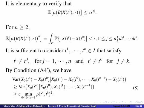
It is elementary to verify thatE[µ(B(X(t0), r)

)]≤ crQ.

For n ≥ 2,

E[µ(B(X(t0), r)

)n]=

∫InP∣∣X(tj)−X(t0)

∣∣ < r, 1 ≤ j ≤ n

dt1 · · · dtn.

It is sufficient to consider t1, · · · , tn ∈ I that satisfy

tj 6= t0, for j = 1, · · · , n and tj 6= tk for j 6= k.

By Condition (A4′), we have

Var(X0(tn)− X0(t0)

∣∣X0(t1)− X0(t0), · · · ,X0(tn−1)− X0(t0))

≥ Var(X0(tn)

∣∣X0(t0),X0(t1), · · · ,X0(tn−1))

≥ c min0≤k≤n−1

ρ(tn, tk)2.

(8)


Since conditional distributions in Gaussian processes arestill Gaussian, it follows from Anderson’s inequality and(8) that∫

IP∣∣X(tn)− X(t0)

∣∣ < r∣∣X(t1)− X(t0), · · · ,X(tn−1)− X(t0)

dtn

≤ c∫

I

n−1∑k=0

min

1, c( rρ(tn, tk)

)ddtn

≤ c n∫

Imin

1, c( rρ(tn, 0)

)ddtn

≤ c nrQ.

Iterating the procedure proves Lemma 5.5.


From Lemma 5.5 and the Borel-Cantelli lemma, we canprove the following law of the iterated logarithm for thesojourn measure of X.

Proposition 5.1For every t0 ∈ I, we have

lim supr→0

µ(B(X(t0), r)

)ϕ5(r)

≤ C <∞, a.s.

This and Fubini’s theorem yield: a.s.

lim supr→0

µ(B(X(t0), r)

)ϕ5(r)

≤ C a.e. t0 ∈ I.

Hence, the lower bound in (7) follows from Lemma 5.1.Yimin Xiao (Michigan State University) Lecture 5. Fractal Properties of Gaussian Random Fields August 2–6, 2021 28 / 44

For proving the upper bound in (7), we need the followingsmall ball probability estimates.

Lemma 5.6 [X. (2009)]Under the conditions of Theorem 5.6, There exist constantsc and c′ such that for all t0 ∈ I = [0, 1]N and 0 < ε < r,

exp(−c′( rε

)Q)≤ P

sup

t∈I:ρ(t,t0)≤r|X(t)−X(t0)| ≤ ε

≤ exp

(−c( rε

)Q).

The main estimate is given in the following lemma.


Proposition 5.2Assume that the conditions of Theorem 5.6 hold. Thereexist positive constants δ0 and C such that for any t0 ∈ Iand 0 < r0 ≤ δ0, we have

P∃ r ∈ [r2

0, r0], supt∈I:ρ(t,t0)≤r

|X(t)− X(t0)| ≤ Cr(

log log(1/r))−1/Q

≥ 1− exp

(−(

log(1/r0)1/2).

Proof. The method of proof comes form Talagrand (1995).We provide the main steps. Let U > 1 be a number whosevalue will be determined later. For k ≥ 0, let rk = r0U−2k.Consider the largest integer k0 such that

k0 ≤log(1/r0)

2 log U.


Thus, for k ≤ k0 we have r20 ≤ rk ≤ r0. It thereby suffices

to prove that

P∃k ≤ k0, sup

t∈I:ρ(t,t0)≤rk

|X(t)− X(t0)| ≤ c rk

(log log

1rk

)−1/Q≥ 1− exp

(−(

log1r0

)1/2).

(9)

Let ak = r−10 U2k−1 and we define for k = 0, 1, · · ·

X0,k(t) = v([ak, ak+1), t)

andXk(t) =

(X1,k(t), · · · ,Xd,k(t)

),

where X1,k(t), · · · ,Xd,k(t) are independent copies of X0,k(t).It follows that X1 − X1,k, · · · ,Xd − Xd,k are independentcopies of X0 − X0,k.


The Gaussian random fields X0, X1, · · · are independent.By Lemma 5.6 we can find a constant c > 0 such that, if r0is small enough, then for each k ≥ 0

P

supt∈I:ρ(t,t0)≤rk

∣∣Xk(t)− Xk(t0)∣∣ ≤ c rk

(log log(1/rk)

)−1/Q

≥ exp(− 1

4log log(1/rk)

)=

1(log 1/rk)1/4

≥(2 log 1/r0

)−1/4.

By the independence,

P∃k ≤ k0, sup

t∈I:ρ(t,t0)≤rk

∣∣Xk(t)− Xk(t0)∣∣ ≤ c rk

(log log(1/rk)

)−1/Q≥ 1−

(1− 1

(2 log 1/r0)1/4

)k0

≥ 1− exp(− k0

(2 log 1/r0)1/4

),

(10)

where the last inequality follows from 1 − x ≤ e−x for allx ≥ 0.Yimin Xiao (Michigan State University) Lecture 5. Fractal Properties of Gaussian Random Fields August 2–6, 2021 32 / 44

To deal with X(t) − Xk(t), we claim that for any u ≥crkU−β

√log U, where β = minHN

−1 − 1, 1,

P

supt∈I:ρ(t,t0)≤rk

∣∣X(t)−Xk(t)−(X(t0)−Xk(t0))∣∣ ≥ u

≤ exp

(− u2

cr2kU−2β

).

(11)To see this, it’s enough to prove that (11) holds for X0, byapplying Lemma 3.3.Consider S = t ∈ I : ρ(t, t0) ≤ rk and on S the distance

d(s, t) =∥∥X0(s)− X0,k(s)− (X0(t)− X0,k(t))

∥∥L2 .

Then d(s, t) ≤ c∑N

i=1 |si− ti|Hi and N(S, d, ε) ≤ c(rk/ε

)Q.


Now we estimate the d-diameter D of S. By Condition(A1), we have for any s, t ∈ S,

‖X0(s)− X0,k(s)− (X0(t)− X0,k(t))‖L2

≤ C( N∑

j=1

aH−1

j −1k |sj − tj|+ a−1

k+1

)≤ CrkU−β,

where β = minHN−1 − 1, 1. Therefore, D ≤ CrkU−β.

Notice that∫ D

0

√log N(S, d, ε)dε ≤ c

∫ CrkU−β

0

√log rk/ε dε

≤ crk

∫ CU−β

0

√log 1/u du ≤ crkU−β

√log U.

Hence (11) follows from Lemma 3.3.


Let U = (log 1/r0)1/β. Then for r0 > 0 small

Uβ (log U)−1/2 ≥(

log log1r0

)1/Q

.

Take u = crk(log log 1/r0)−1/Q. It follows from (11) that

P

supt∈I:ρ(t, t0)≤rk

∣∣X(t)− Xk(t)−(X(t0)− Xk(t0)

)∣∣ ≥ c rk(

log log1r0

)−1/Q

≤ exp(− cUβ

(log log 1/r0)2/Q

).


Combining this with (10), we get

P∃k ≤ k0, sup

ρ(t, t0)≤rk

∣∣X(t)− X(t0)∣∣ ≤ c rk

(log log(1/rk

)−1/Q

≥ 1− exp(− k0

(2 log 1/r0)1/4

)− k0 exp

(− cUβ

(log log 1/r0)2/Q

).

This proves (9) and Proposition 5.2.

With Proposition 5.2 in hand, we proceed to constructionof an economic covering for X([0, 1]N).


For k ≥ 1, consider the set

Rk =

t ∈ [0, 1]N : ∃ r ∈ [2−2k, 2−k] such that

sups∈I:ρ(s,t)≤r

∣∣X(s)− X(t)∣∣ ≤ c r(log log

1r

)−1/Q

.

By Lemma 5.7 we have that for every t ∈ [0, 1]N ,

Pt ∈ Rk ≥ 1− exp(−√

k/2).

This and Fubini’s theorem imply that

E[λN(Rk)] ≥ 1− exp(−√

k/2).

OrE[λN(I\Rk)] ≤ exp(−

√k/2).


By Markov’s inequality, we have

PλN(Rk) < 1− exp(−

√k/2)

= P

λN(I\Rk) > exp(−

√k/2)

≤ E[λN(I\Rk)]

exp(−√

k/2)

≤ exp(−( 1√

2− 1

2

)√k).

Hence, by the Borel-Cantelli lemma, we have P(Ω1) = 1,where

Ω1 =ω : λN(Rk) ≥ 1− exp(−

√k/2) for all k large enough

.


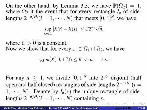
On the other hand, by Lemma 3.3, we have P(Ω2) = 1,where Ω2 it the event that for every rectangle In of side-lengths 2−n/Hi(i = 1, · · · ,N) that meets [0, 1]N , we have

sups,t∈In

∣∣X(t)− X(s)∣∣ ≤ C2−n√n,

where C > 0 is a constant.Now we show that for every ω ∈ Ω1 ∩ Ω2, we have

ϕ5-m(X([0, 1]N)) ≤ K <∞, a.s.

For any n ≥ 1, we divide [0, 1]N into 2nQ disjoint (halfopen and half closed) rectangles of side-lengths 2−n/Hi (i =1, · · · ,N). Denote by In(x) the unique rectangle of side-lengths 2−n/Hi(i = 1, · · · ,N) containing x.


Consider k ≥ 1 such that

λN(Rk) ≥ 1− exp(−√

k/2).

For any x ∈ Rk we can find the smallest integer n withk ≤ n ≤ 2k such that

sups,t∈In(x)

∣∣X(t)− X(s)∣∣ ≤ c 2−n(log log 2n)−1/Q. (12)

Thus we have

Rk ⊆ V =2k⋃

n=k

Vn

and each Vn is a union of rectangles In(x) satisfying (12).Notice that X(In(x)) can be covered by a ball of radius rn =c2−n(log log 2n)−1/Q.


Since ϕ5(2rn) ≤ c2−nQ = cλN(In), we obtain

2k∑n=k

∑In∈Vn

ϕ5(2rn) ≤∑

n

∑In∈Vn

cλN(In) = CλN(V) ≤ C. (13)

Thus X(V) is contained in the union of a family of balls Bnof radius rn with

∑n ϕ5(2rn) ≤ C.

On the other hand, [0, 1]N\V is contained in a union ofrectangles of side-lengths 2−q/Hi(i = 1, · · · ,N) where q =2k + 1, none of which meets Rk. There can be at most

2QqλN([0, 1]N\V) ≤ c2Qq exp(−√

k/2)

such rectangles.


Since ω ∈ Ω2, for each of these rectangles Iq, X(Iq) iscontained in a ball of radius c2−q√q.Thus X([0, 1]N\V) can be covered by a sequence Bn ofballs of radius rn = c2−q√q such that∑

n

ϕ5(2rn) ≤(

c2Qq exp(−√

k/2))(

c2−qQqQ/2 log log(c2q/√

q))

≤ 1(14)

for all k large enough. Since k can be arbitrarily large, itfollows from (13) and (14) that

ϕ5-m(X([0, 1]N)

)≤ K, a.s.

This finishes the proof of Part (i) of Theorem 5.6.Part (ii) is related to the existence of local times. A proofbased on Fourier analysis will be given in Lecture 6.


If Condition (A4′) in Theorem 5.6 is replaced by (A4), thenthe exact Hausdorff measure function for X([0, 1]N) is dif-ferent. See the recent paper of Lee (2021).


Thank you


Lecture 5. Fractal Properties of Gaussian Random Fields

Documents

Transcript of Lecture 5. Fractal Properties of Gaussian Random Fields