Lecture 4.Engr 691-73 Introduction to Free-Surface Hydraulics in Open Channels1 ENGR 691 – 73:...
68
Lecture 4. Engr 691-73 Introduction to Free-Surface Hydraulics in Open Channels 1 ENGR 691 – 73: Introduction to Free-Surface Hydraulics in Open Channels Lecture 04: Nonuniform Flow Course Notes by: Mustafa S. Altinakar and Yan Ding Yan Ding, Ph.D. Research Assistant Professor, National Center for Computational Hydroscience and Engineering (NCCHE), The University of Mississippi, Old Chemistry 335, University, MS 38677 Phone: 915-8969; Email: [email protected]
-
Upload
tre-unthank -
Category
Documents
-
view
277 -
download
15
Transcript of Lecture 4.Engr 691-73 Introduction to Free-Surface Hydraulics in Open Channels1 ENGR 691 – 73:...

Lecture 4. Engr 691-73 Introduction to Free-Surface Hydraulics in Open Channels 1
ENGR 691 – 73: Introduction to Free-Surface Hydraulics in Open Channels
Lecture 04: Nonuniform Flow
Course Notes by: Mustafa S. Altinakar and Yan Ding
Yan Ding, Ph.D. Research Assistant Professor, National Center for Computational
Hydroscience and Engineering (NCCHE), The University of Mississippi, Old Chemistry 335, University, MS 38677
Phone: 915-8969; Email: [email protected]

Lecture 4. Engr 691-73 Introduction to Free-Surface Hydraulics in Open Channels 2
Outline
• Transition Between Subcritical and Critical Flow• Introduction to Hydraulic Jump• Gradually Varied Flow (Governing Equations)• Forms of water surface (Channels on Mild Slope, Critical Slope,
Steep Slope, Adverse Slope, Horizontal Slope)• Control Points• Computation of Water Surface (Method of successive
Approximations; Method of Direct Integration; Method of Graphical Integration)
• Rapidly Varied Flow (Weirs; Spillways; Hydraulic Drop; Underflow Gates; Hydraulic Jump)
• Transitions (Channel with variable Bed Floor; Channel of variable Width; Oblique Jump)
• Lateral Inflow

Lecture 4. Engr 691-73 Introduction to Free-Surface Hydraulics in Open Channels 3
co SS
co SS
Transitionfrom subcritical to supercritical flow
When the flow changes from subcritical to supercritical the water surface lowers gradually from a higher depth to a lower depth by passing through critical depth.
In the region where the flow changes from subcritical to critical flow, a gradually varied flow takes place.
Transitionfrom supercritical to subcritical flow
When the flow changes from supercritical to subcritical the water surface rapidly increases from a supercritical depth to subcritical depth. This sudden increase is called a rapidly varied flow.
The rapidly varied flow may be preceded by a gradually varied flow region where the flow depth rises but stays below critical depth.
co SS
co SS
Transitions between subcritical and critical flow

Lecture 4. Engr 691-73 Introduction to Free-Surface Hydraulics in Open Channels 4
1sH
h
Specific Energyg
VhH s 2
2
1h
2h
ch
2sH hjh
conjugate depthsorsequent depths
sHM
h
21 MM
Specific Momentum
2
22 h
gh
qM
1h
2h
ch
q
1h 2h1V
2V
2211 hVhVq Equation of continuity
1221VVQFFF pp Momentum equation
with Bh
Fp 2
21
1 B
hFp 2
22
2
alternate depths
hjh
Things to remember:• Conjugate depths or
sequent depths (on Specific Momentum Curve)
• Alternate depths (on Specific Energy Curve)
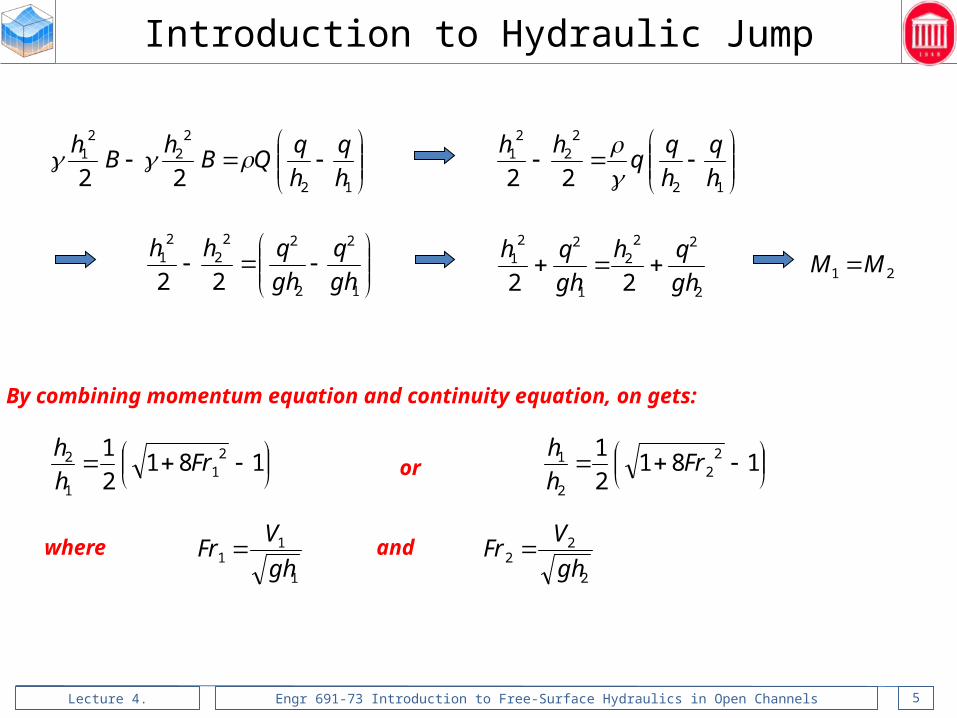
Introduction to Hydraulic Jump
Lecture 4. Engr 691-73 Introduction to Free-Surface Hydraulics in Open Channels 5
12
22
21
22 h
q
h
qQB
hB
h
12
22
21
22 h
q
h
hh
1
2
2
222
21
22 gh
q
gh
qhh
2
222
1
221
22 gh
qh
gh
qh 21 MM
By combining momentum equation and continuity equation, on gets:
181
2
1 21
1
2 Frh
hor
181
2
1 22
2
1 Frh
h
where1
11
gh
VFr
2
22
gh
VFr and
Introduction to Hydraulic Jump

Lecture 4. Engr 691-73 Introduction to Free-Surface Hydraulics in Open Channels 6
Q1h
1z
gU 2/21
2h
2z
gU 2/22
ref. line
fh
L
Consider the steady non uniform flow in a channel. We wish to develop an equation for the variation of the water surface h(x), i.e. longitudinal water surface profile.
For this, we will consider the equation of energy:
H
g
AQhz
g
Uhz
2
/
2
22
and the equation of continuity: UAQ
h
z
gU 2/2
H
Differentiate the energy equation with respect to x to get:
dx
dH
g
AQ
dx
d
dx
dh
dx
dz
2
/ 2
oS eS
Assuming that the head loss can be expressed using Chezy equation, we have:
he RC
AQS
2
2/
h
o RC
AQS
dx
dh
g
AQ
dx
d2
22 /
2
/
Gradually Varied Flow Equation

Lecture 4. Engr 691-73 Introduction to Free-Surface Hydraulics in Open Channels 7
Q1h
1z
gU 2/21
2h
2z
gU 2/22
ref. line
fh
L
Consider the steady non uniform flow in a channel. We wish to develop an equation for the variation of the water surface h(x), i.e. longitudinal water surface profile.
For this, we will consider the equation of energy:
H
g
AQhz
g
Uhz
2
/
2
22
and the equation of continuity: UAQ
h
z
gU 2/2
H
Differentiate the energy equation with respect to x to get:
dx
dH
g
AQ
dx
d
dx
dh
dx
dz
2
/ 2
oS eS
Assuming that the head loss can be expressed using Chezy equation, we have:
he RC
AQS
2
2/
h
o RC
AQS
dx
dh
g
AQ
dx
d2
22 /
2
/
Gradually Varied Flow Equation
Lecture 4. Engr 691-73 Introduction to Free-Surface Hydraulics in Open Channels 8
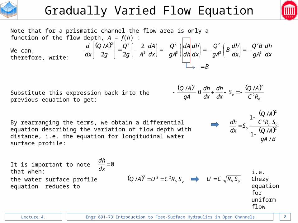
Note that for a prismatic channel the flow area is only a function of the flow depth, A = f(h) :
We can, therefore, write:
dx
dh
gA
BQ
dx
dhB
gA
Q
dx
dh
dh
dA
gA
Q
dx
dA
Ag
Q
g
AQ
dx
d3
2
3
2
3
2
3
22 2
22
/
B
h
o RC
AQS
dx
dh
dx
dhB
gA
AQ2
22 //Substitute this expression back into the previous equation to get:
By rearranging the terms, we obtain a differential equation describing the variation of flow depth with distance, i.e. the equation for longitudinal water surface profile:
BgA
AQ
SRCAQ
Sdx
dh oho
//
1
/1
2
2
2
It is important to note that when: 0dx
dh
the water surface profile equation reduces to oh SRCUAQ 222/ oh SRCU i.e. Chezy equation for uniform flow
Gradually Varied Flow Equation

Lecture 4. Engr 691-73 Introduction to Free-Surface Hydraulics in Open Channels 9
Consider again the equation for longitudinal water surface profile:
BgA
AQ
SRCAQ
Sdx
dh oho
//
1
/1
2
2
2
For
BgA
AQ
/
/1
2
the denominator becomes zero and we have: dx
dh
hgD
U 2
1 21 Fr
We can, therefore conclude that, at critical flow (Fr = 1 and h = hc), the water surface profile is perpendicular to bed.
The normal is equal to critical depth, hn = hc , when:
BgA
AQ
SRC
AQ
oh /
/10
/1
2
2
2
BgASRC oh /2
0dx
dhUniform flow
1Fr
0dx
dh
0dx
dh
0dx
dh
The flow depth remains constant and is equal to normal depth (uniform flow)
The flow depth increases in the direction of flow
The flow depth decreases in the direction of flow
Gradually Varied Flow Equation

Lecture 4. Engr 691-73 Introduction to Free-Surface Hydraulics in Open Channels 10
Consider the flow cases below (for all cases channel cross section characteristics are the same):
chnh
ch
nh
nc hh
co SS co SS co SS
cn hh cn hh cn hh
1Fr 1Fr 1Fr
Critical slope is the bed slope when normal depth, hn, is equal to critical depth, hc.
When flow is critical, we have: 1hgD
UFr 1
BA
gA
QFr 1
3
2
gA
BQ
B
gAQ
32
Since the flow is also uniform, Chezy equation holds:2/12/1
oh SRCAQ
Equating two expressions, we have:B
gASRACQ ch
3222 note that we have changed So to Sc.
hc BRC
gAS
2The expression for critical discharge is obtained as:
If Manning-Strickler is used:B
gASR
n
AQ ch
33/4
2
22 3/4
2
h
cBR
gAnS
Review of the Notion of Critical Flow

Lecture 4. Engr 691-73 Introduction to Free-Surface Hydraulics in Open Channels 11
The gradually varied flow equation can therefore be written as:
c
on
n
o
SS
KK
KK
Sdx
dh2
2
1
1
The equation for gradually varied flow can also be written using the notion of conveyance:
Remember the definition of conveyance:
3/2)( hRn
AhK
2/1)( hRAChK
when using Manning Strickler
when using Chezy
2/1)( on ShKQ
2
2
2
2
22/1
2
22
2
2
2/
K
K
SK
SK
SCAR
Q
SRAC
Q
SRC
AQ n
o
on
ohohoh
3
22
/
/
gA
BQ
BgA
AQ
Consider the term in the denominator of gradually varied flow equation: 3
222
222
2
3
2
gA
SRAC
SRAC
BQ
gA
BQ oh
oh
oh
ho
SgA
RBC
CARS
Q
gA
BQ 22
22/1
2
3
2 1
when the flow is uniform, in either case we can write:
cS
1
or
2/1)(o
nS
QhK
2)(hKn )(hK
c
on
S
S
K
K
gA
BQ2
2
3
2
Now consider the term in the nominator of gradually varied flow equation:
Gradually Varied Flow Equation in Terms of Conveyance
Lecture 4. Engr 691-73 Introduction to Free-Surface Hydraulics in Open Channels 12
3
3
1
1
hh
hh
Sdx
dh
c
n
o
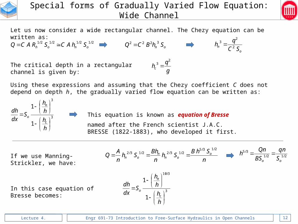
Let us now consider a wide rectangular channel. The Chezy equation can be written as:
2/12/12/12/1onoh ShACSRACQ
on SC
qh
2
23
The critical depth in a rectangular channel is given by:g
qhc
23
Using these expressions and assuming that the Chezy coefficient C does not depend on depth h, the gradually varied flow equation can be written as:
This equation is known as equation of Bresse
If we use Manning-Strickler, we have:n
ShBSh
n
BhSh
n
AQ o
onn
on
2/13/52/13/22/13/2 2/12/1
3/5
oo S
qn
BS
Qnh
on ShBCQ 3222
In this case equation of Bresse becomes: 3
3/10
1
1
hh
hh
Sdx
dh
c
n
o
named after the French scientist J.A.C. BRESSE (1822-1883), who developed it first.
Special forms of Gradually Varied Flow Equation: Wide Channel

Lecture 4. Engr 691-73 Introduction to Free-Surface Hydraulics in Open Channels 13
Before we present all possible gradually varied flow profiles, let us take a look at the general properties of such curves:• The water surface profile approaches asymptotically to uniform depth hn.
• The water surface profile is orthogonal to the critical depth line, when h = hc.
Water surface profiles are classified according to the bed slope.
0oS
0oS
0oS
co SS
co SS
co SS
Channel on Mild slope M
Channel on Steep slope S
Channel on Critical slope C
Channel on Horizontal slope H
Channel on Adverse slope A
type profile
type profile
type profile
type profile
type profile
For each profile type several possibilities are distinguished. These are called branches.
In studying gradually varied water surface profiles we should also keep in mind that:
• In subcritical flow (Fr < 1), the perturbations travel both upstream and downstream. The water surface profiles for subcritical flow are controlled by a downstream control section.
• In supercritical flow (Fr > 1), the perturbations travel only downstream. The water surface profiles for supercritical flow are controlled by an upstream control section.
Gradually Varied Flow: Forms of Water Surface

Lecture 4. Engr 691-73 Introduction to Free-Surface Hydraulics in Open Channels 14
Convention for numbering branches:
• When the water surface profile is higher than both the normal depth and the critical depth, the branch is numbered as type 1,
• the water surface profile is between the normal and critical depths, the branch is numbered as type 2,
• the water surface profile is lower than both the normal depth and the critical depth, the branch is numbered as type 3,
Gradually Varied Flow: Forms of Water Surface

Lecture 4. Engr 691-73 Introduction to Free-Surface Hydraulics in Open Channels 15
0oS co SS
Channel on Mild slope
M-type profiles
and
cn hhh
1Fr
0dx
dh
Branch M1
cn hhh
1Fr
0dx
dh
Branch M2
hhh cn
1Fr
0dx
dh
Branch M3
Towards upstream the profile approaches asymptotically
normal depth, towards downstream the curve tends to
become horizontal.
Encountered:• Upstream of a weir or a dam• Upstream of a pier• Upstream of certain bed
slope changes points
Towards upstream the profile approaches asymptotically
normal depth, towards downstream the curve
decreasingly tends to critical depth.
Encountered:• Upstream of an increase in
bed slope• Upstream of a free drop
structure
Towards downstream the profile approaches increasingly
to critical depth.
Encountered:• When a supercritical flow
enters a mild channel• After a change in slope from
steep to mild
cn hh
Gradually Varied Flow: Forms of Water Surface

Lecture 4. Engr 691-73 Introduction to Free-Surface Hydraulics in Open Channels 16
0oS co SS
Channel on Steep slope
S-type profiles
and
nc hhh
1Fr
0dx
dh
Branch S1
nc hhh
1Fr
0dx
dh
Branch S2
hhh nc
1Fr
0dx
dh
Branch S3
Towards upstream the profile approaches asymptotically
normal depth, towards downstream the curve tends to
become horizontal.
Encountered:• Upstream of a weir or a dam• Upstream of a pier• Upstream of certain bed
slope changes points
Towards upstream the profile approaches asymptotically
normal depth, towards downstream the curve
decreasingly tends to critical depth.
Encountered:• Upstream of an increase in
bed slope• Upstream of a free drop
structure
Towards downstream the profile approaches increasingly
to critical depth.
Encountered:• When a supercritical flow
enters a mild channel• After a change in slope from
steep to mild
cn hh
Gradually Varied Flow: Forms of Water Surface

Lecture 4. Engr 691-73 Introduction to Free-Surface Hydraulics in Open Channels 17
0oS co SS
Channel on Critical slope
C-type profiles
and
nc hhh
1Fr
0dx
dh
Branch C1 Branch C2
nc hhh
1Fr
0dx
dh
Branch C3
The water surface profile is horizontal, when Chezy
equation is used.
Encountered:• Upstream of a dam/weir• At certain bed slope change
locations
There is no physically possible C2 profile.
The water surface profile is horizontal, when Chezy
equation is used.
Encountered:• When a supercritical flow
enters a mild channel• After a change in slope from
steep to mild
cn hh
Gradually Varied Flow: Forms of Water Surface

Lecture 4. Engr 691-73 Introduction to Free-Surface Hydraulics in Open Channels 18
0oS
Channel on Horizontal slope
H-type profiles
Branch H1
chh
1Fr
0dx
dh
Branch H2
hhc
1Fr
0dx
dh
Branch H3
Normal depth becomes infinite and is meaningless.
Consequently, H1 profile is not possible.
Similar to M2 profile
Encountered:• Upstream of a free drop
structure
Similar to M3 profile
Encountered:• When a supercritical flow
enters a horizontal channel
nh
Gradually Varied Flow: Forms of Water Surface

Lecture 4. Engr 691-73 Introduction to Free-Surface Hydraulics in Open Channels 19
0oS
Channel on Adverse slope
H-type profiles
Branch A1 Branch A2 Branch A3
Normal depth becomes infinite and is meaningless.
Consequently, A1 profile is not possible.
Similar to H2 profile (parabolic)
Encountered:• Upstream of a certain bed
slope change location
Similar to H3 profile(parabolic)
Encountered:• When a supercritical flow
enters a channel with adverse slope
nh
chh
1Fr
0dx
dh
hhc
1Fr
0dx
dh
Gradually Varied Flow: Forms of Water Surface
Lecture 4. Engr 691-73 Introduction to Free-Surface Hydraulics in Open Channels 20
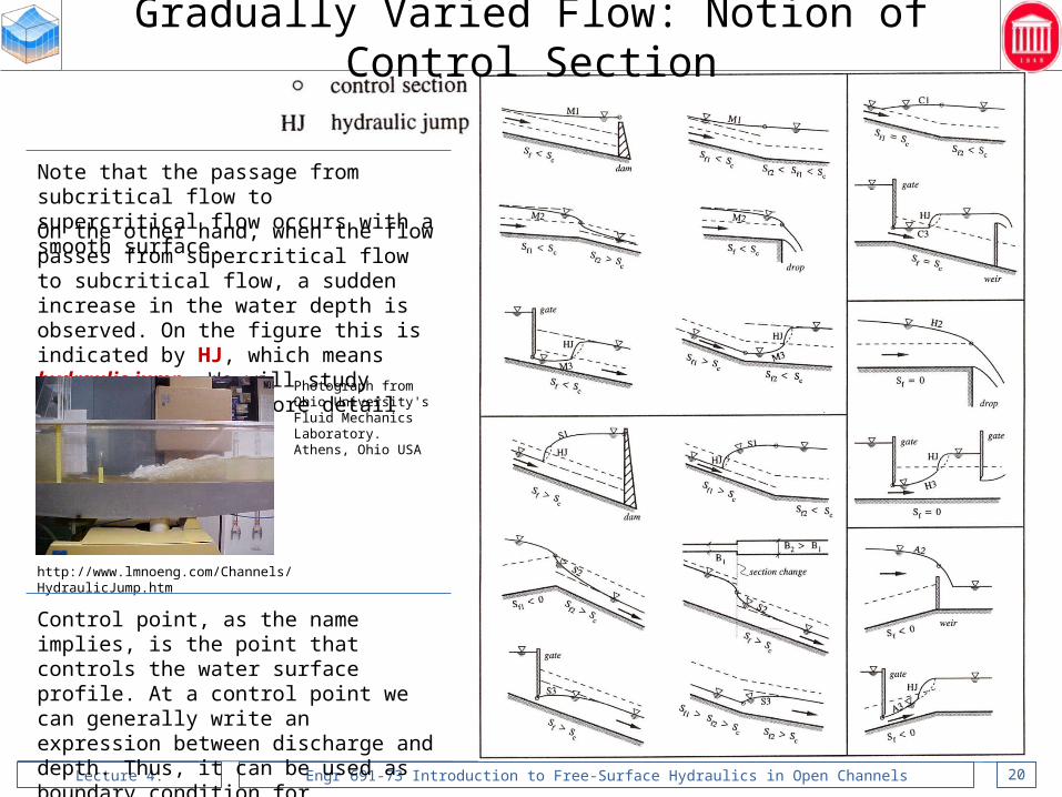
Note that the passage from subcritical flow to supercritical flow occurs with a smooth surface.
On the other hand, when the flow passes from supercritical flow to subcritical flow, a sudden increase in the water depth is observed. On the figure this is indicated by HJ, which means hydraulic jump. We will study hydraulic jump in more detail later.
http://www.lmnoeng.com/Channels/HydraulicJump.htm
Photograph from Ohio University's Fluid Mechanics Laboratory. Athens, Ohio USA
Control point, as the name implies, is the point that controls the water surface profile. At a control point we can generally write an expression between discharge and depth. Thus, it can be used as boundary condition for calculating the water surface profile.
Gradually Varied Flow: Notion of Control Section
Lecture 4. Engr 691-73 Introduction to Free-Surface Hydraulics in Open Channels 21
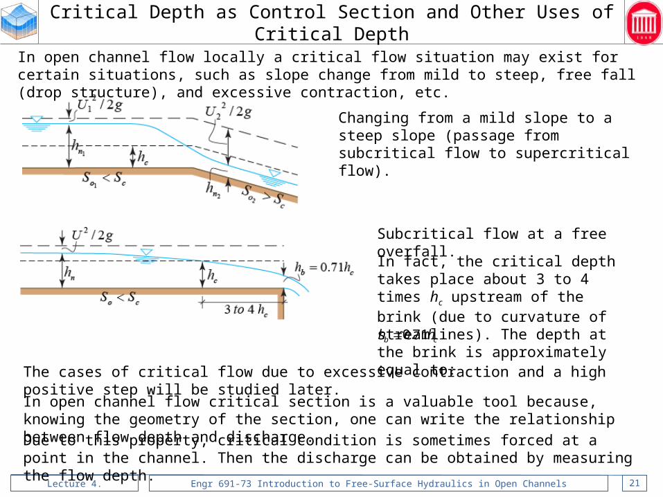
Changing from a mild slope to a steep slope (passage from subcritical flow to supercritical flow).
Subcritical flow at a free overfall.
In open channel flow critical section is a valuable tool because, knowing the geometry of the section, one can write the relationship between flow depth and discharge.
Due to this property, critical condition is sometimes forced at a point in the channel. Then the discharge can be obtained by measuring the flow depth.
cb hh 71.0
In open channel flow locally a critical flow situation may exist for certain situations, such as slope change from mild to steep, free fall (drop structure), and excessive contraction, etc.
In fact, the critical depth takes place about 3 to 4 times hc upstream of the brink (due to curvature of streamlines). The depth at the brink is approximately equal to:
The cases of critical flow due to excessive contraction and a high positive step will be studied later.
Critical Depth as Control Section and Other Uses of Critical Depth

Lecture 4. Engr 691-73 Introduction to Free-Surface Hydraulics in Open Channels 22
x
c
n
o hxf
hh
hh
Sdx
dh,
1
1
3
3
Several methods are available for computing gradually varied water surface profiles:
1. The most obvious is to solve the differential equation of gradually varied flow, equation of Bresse, using a numerical method, such as 4th order Runge-Kutta method. This method is called method of direct integration.
Equation of Bresse using Chezy equation:
Equation of Bresse using Manning-Strickler equation:
4th order Runge-Kutta method formula can be written as: 4321 226
kkkkx
hh xxx
where: x Coordinate along the channel length. The origin can be arbitrarily placed at any location.
xh Flow depth at location x. All flow parameters at this location are known.
xxh Flow depth at location x+Dx. This is the unknown flow depth we are calculating.
x
c
n
o hxf
hh
hh
Sdx
dh,
1
1
3
3/10
xhxfk ,1
12 2,
2k
xh
xxfk x
23 2,
2k
xh
xxfk x
34 , kxhxxfk x
Computations should start from a point where all flow parameters are known (such as a control point) and proceed upstream if the flow is subcritical and downstream if the flow is supercritical.
Computation of Gradually Varied Flow
Lecture 4. Engr 691-73 Introduction to Free-Surface Hydraulics in Open Channels 23
Several methods are available for computing gradually varied water surface profiles:
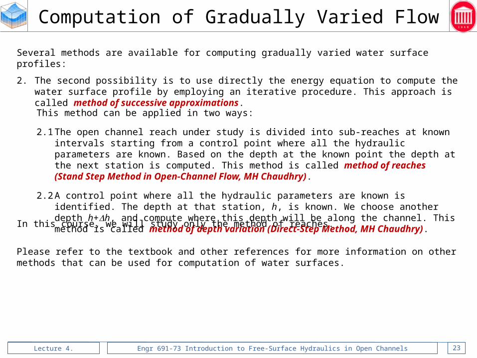
2. The second possibility is to use directly the energy equation to compute the water surface profile by employing an iterative procedure. This approach is called method of successive approximations.
This method can be applied in two ways:
2.1 The open channel reach under study is divided into sub-reaches at known intervals starting from a control point where all the hydraulic parameters are known. Based on the depth at the known point the depth at the next station is computed. This method is called method of reaches (Stand Step Method in Open-Channel Flow, MH Chaudhry).
2.2 A control point where all the hydraulic parameters are known is identified. The depth at that station, h, is known. We choose another depth h+Dh, and compute where this depth will be along the channel. This method is called method of depth variation (Direct-Step Method, MH Chaudhry).
In this course, we will study only the method of reaches.
Please refer to the textbook and other references for more information on other methods that can be used for computation of water surfaces.
Computation of Gradually Varied Flow
Lecture 4. Engr 691-73 Introduction to Free-Surface Hydraulics in Open Channels 24
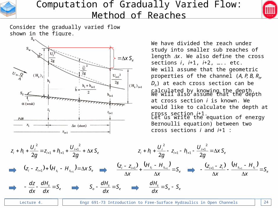
Consider the gradually varied flow shown in the figure.
eSx
We have divided the reach under study into smaller sub reaches of length Dx. We also define the cross sections i, i+1, i+2, ….. etc.
We will assume that the geometric properties of the channel (A, P, B, Rh, Dh) at each cross section can be calculated by knowing the depth.
We will also assume that the depth at cross section i is known. We would like to calculate the depth at cross section i+1.
Let us write the equation of energy Bernoulli equation) between two cross sections i and i+1 :
ei
iii
ii Sxg
Uhz
g
Uhz
22
21
11
2
ei
iii
ii Sxg
Uhz
g
Uhz
22
21
11
2
essii SxHHzzii
11
e
ssii Sx
HH
x
zzii
11
essii S
x
HH
x
zzii
11
es S
dx
dH
dx
dz e
so S
dx
dHS eo
s SSdx
dH
Computation of Gradually Varied Flow: Method of Reaches

Lecture 4. Engr 691-73 Introduction to Free-Surface Hydraulics in Open Channels 25
Therefore, when using the method of reaches, we will be solving this ordinary differential equation:
eSx
The basic equation we are using is:
ei
iii
ii Sxg
Uhz
g
Uhz
22
21
11
2
Since depth hi , invert elevation zi and the discharge Q are known, we can calculate the left side of the equation, i.e. the total energy head, Hi directly.
eii SxHH 1
Let us now assume a depth hi+1 . Since the invert elevation zi and the discharge Q are known, we can also calculate the total energy head, Hi+1 directly.
Now the question is weather the assumed that is the correct depth. This can be easily done. If the assumed depth hi+1 is correct, then, the difference between the total heads Hi and Hi+1 should be equal to Dx Se.
The energy gradient can be calculated using either the equation of Chezy or Manning Strickler:
h
e RC
AQS
2
2/Chezy equation: Manning Strickler equation:
3/4
22/
h
eR
nAQS
Computation of Gradually Varied Flow

Lecture 4. Engr 691-73 Introduction to Free-Surface Hydraulics in Open Channels 26
Since the hydraulic parameters are varying from cross section i to i+1, we may want to use the average value of the energy gradient:
21
ii ee
e
SSS
Note also that : ii xxx 1
We should therefore check that: eii SxHH 1 or
21
11ii ee
iiii
SSxxHH is satisfied.
If the above equation is not satisfied, a new value should be assumed for hi+1 and the computations must be carried out again.
All these calculation can easily be carried out on a spread sheet.
If there are singular losses between the two cross sections i and i +1, this should also be taken into account. Then the equation becomes:
g
AQKSx
g
UKSxHH eeii 2
/
2
22
1
Again considering average values we can write:
2
//
2
1
2
21
2
111
iiee
iiii
AQAQ
gK
SSxxHH ii
2
//
2
1
2
/ 21
22
ii AQAQ
gg
AQ
Consequently:
Computation of Gradually Varied Flow

Lecture 4. Engr 691-73 Introduction to Free-Surface Hydraulics in Open Channels 27
The computation of gradually varied flow equations can be easily carried out on a spreadsheet using Goal Seek function
A trapezoidal channel having a bottom width of b = 7.0m and side slopes of m = 1.5, conveys a discharge of Q = 28m3/s. The channel has a constant bed slope of So = 0.001. The Manning friction coefficient for the channel is n = 0.025m-1/3s. The channel terminates by a sudden drop of the bed.1. Determine the type of water surface profile to be expected.2. Calculate the water surface profile for a reach length of 3200m.
Computation of Gradually Varied Flow
Lecture 4. Engr 691-73 Introduction to Free-Surface Hydraulics in Open Channels 28
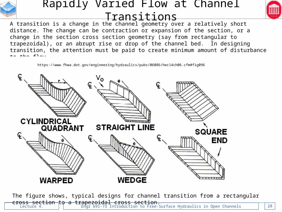
A transition is a change in the channel geometry over a relatively short distance. The change can be contraction or expansion of the section, or a change in the section cross section geometry (say from rectangular to trapezoidal), or an abrupt rise or drop of the channel bed. In designing transition, the attention must be paid to create minimum amount of disturbance to the flow.
https://www.fhwa.dot.gov/engineering/hydraulics/pubs/06086/hec14ch06.cfm#fig096
The figure shows, typical designs for channel transition from a rectangular cross section to a trapezoidal cross section.
Rapidly Varied Flow at Channel Transitions

Lecture 4. Engr 691-73 Introduction to Free-Surface Hydraulics in Open Channels 29
ss HE
gU 2/22
chh 1
gU c 2/2ch
gU 2/21
1h
ch
chh 2
Alternate depths
ss HorE
h
Specific Energy
Curve plotted for a constant Q
Subcrit
ical f
low
Supercritical flow
2
22
22 gA
Qh
g
UhH s
Specific energy curve is an extremely useful tool for analyzing various flow situations. In the following slides we will learn how the specific energy curve can be used to analyze various flow situations in channel transitions (flow over a positive or negative step, flow through a contraction or expansion).
2h
Use of Specific Energy to study Rapidly Varied Flow at Channel Transitions

Lecture 4. Engr 691-73 Introduction to Free-Surface Hydraulics in Open Channels 30
In the following pages we will study in detail the rapid change of water surface at four types of channel transitions under both subcritical and supercritical conditions:
1. Subcritical flow over a positive step
2. Supercritical flow over a positive step
3. Subcritical flow over a negative step
4. Supercritical flow over a negative step
5. Subcritical flow through a contraction
6. Supercritical flow through a contraction
7. Subcritical flow through an expansion
8. Supercritical flow through an expansion
z
z
Side view
Side view
Top view
Top view
Q
Q
Q
Q
Rapidly Varied Flow at Channel Transitions

Lecture 4. Engr 691-73 Introduction to Free-Surface Hydraulics in Open Channels 31
zzH s 1
1sH
z2h
1h
h
sH
2sH
gU 2/21
zH s 1
2sH
2h
h
sH
gU 2/22
./ constBQq
./ constBQq
ch
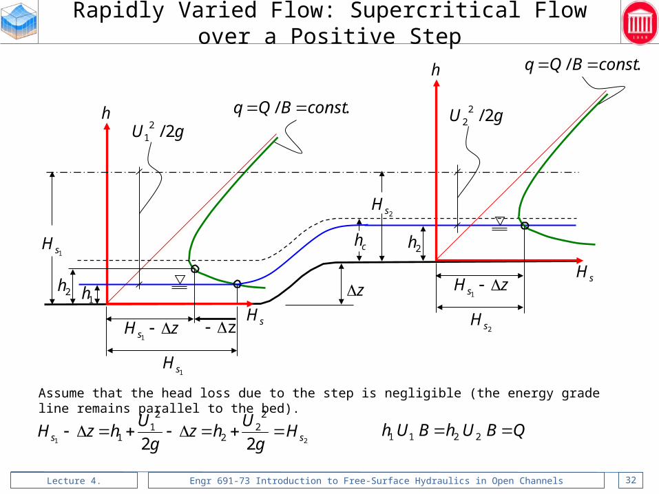
Assume that the head loss due to the step is negligible (the energy grade line remains parallel to the bed).
QBUhBUh 2211
1sH
21 22
22
2
21
1 ss Hg
Uhz
g
UhzH
Rapidly Varied Flow: Subcritical Flow over a Positive Step
Lecture 4. Engr 691-73 Introduction to Free-Surface Hydraulics in Open Channels 32
zzH s 1
1sH
z2h1h
h
sH
1sH
gU 2/21
./ constBQq
ch
Assume that the head loss due to the step is negligible (the energy grade line remains parallel to the bed).
QBUhBUh 2211
zH s 1
2sH
2h
h
sH
2sH
gU 2/22
./ constBQq
21 22
22
2
21
1 ss Hg
Uhz
g
UhzH
Rapidly Varied Flow: Supercritical Flow over a Positive Step

Lecture 4. Engr 691-73 Introduction to Free-Surface Hydraulics in Open Channels 33
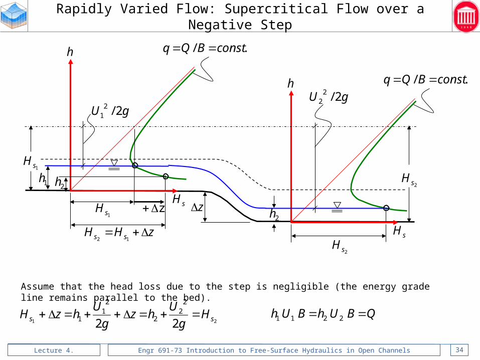
zz
zHH ss 12
1sH
1h
2h
h
sH
gU 2/21
./ constBQq
1sH
2sH
2h
h
sH
gU 2/22
./ constBQq
2sH
Assume that the head loss due to the step is negligible (the energy grade line remains parallel to the bed).
21 22
22
2
21
1 ss Hg
Uhz
g
UhzH QBUhBUh 2211
Rapidly Varied Flow: Subcritical Flow over a Negative Step
Lecture 4. Engr 691-73 Introduction to Free-Surface Hydraulics in Open Channels 34
zz
zHH ss 12
1sH
1h2h
h
sH
gU 2/21
./ constBQq
1sH
2sH
2h
h
sH
gU 2/22
./ constBQq
2sH
Assume that the head loss due to the step is negligible (the energy grade line remains parallel to the bed).
21 22
22
2
21
1 ss Hg
Uhz
g
UhzH QBUhBUh 2211
Rapidly Varied Flow: Supercritical Flow over a Negative Step

Lecture 4. Engr 691-73 Introduction to Free-Surface Hydraulics in Open Channels 35
1sH
1ch
1h
h
sH
gU 2/21
11 / BQq
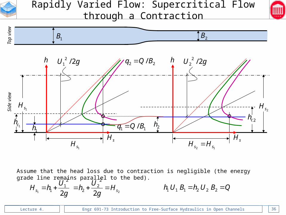
Assume that the head loss due to contraction is negligible (the energy grade line remains parallel to the bed).
QBUhBUh 222111
1sH
21 22
22
2
21
1 ss Hg
Uh
g
UhH
2h
h
sH
gU 2/2222 / BQq
2sH
1B 2B
Top
view
Side
vie
w
12 ss HH
2ch
Rapidly Varied Flow: Subcritical Flow through a Contraction
Lecture 4. Engr 691-73 Introduction to Free-Surface Hydraulics in Open Channels 36
1sH
1ch1h
h
sH
gU 2/21
11 / BQq
Assume that the head loss due to contraction is negligible (the energy grade line remains parallel to the bed).
QBUhBUh 222111
1sH
21 22
22
2
21
1 ss Hg
Uh
g
UhH
12 ss HH
2h
h
sH
gU 2/2222 / BQq
2sH
1B 2B
Top
view
Side
vie
w
2ch
Rapidly Varied Flow: Supercritical Flow through a Contraction
Lecture 4. Engr 691-73 Introduction to Free-Surface Hydraulics in Open Channels 37
1sH
1ch
1h
h
sH
gU 2/21
22 / BQq
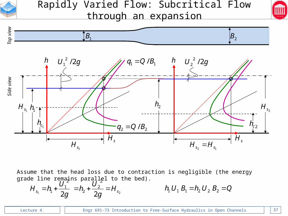
Assume that the head loss due to contraction is negligible (the energy grade line remains parallel to the bed).
QBUhBUh 222111
1sH
21 22
22
2
21
1 ss Hg
Uh
g
UhH
2h
h
sH
gU 2/2211 / BQq
2sH
1B 2B
Top
view
Side
vie
w
12 ss HH
2ch
Rapidly Varied Flow: Subcritical Flow through an expansion

Lecture 4. Engr 691-73 Introduction to Free-Surface Hydraulics in Open Channels 38
Rapidly Varied Flow: Supercritical Flow through an Expansion
1sH
1ch1h
h
sH
gU 2/21
22 / BQq
Assume that the head loss due to contraction is negligible (the energy grade line remains parallel to the bed).
QBUhBUh 222111
1sH
21 22
22
2
21
1 ss Hg
Uh
g
UhH
2h
h
sH
gU 2/2211 / BQq
2sH
1B 2B
Top
view
Side
vie
w
2ch
12 ss HH
Lecture 4. Engr 691-73 Introduction to Free-Surface Hydraulics in Open Channels 39
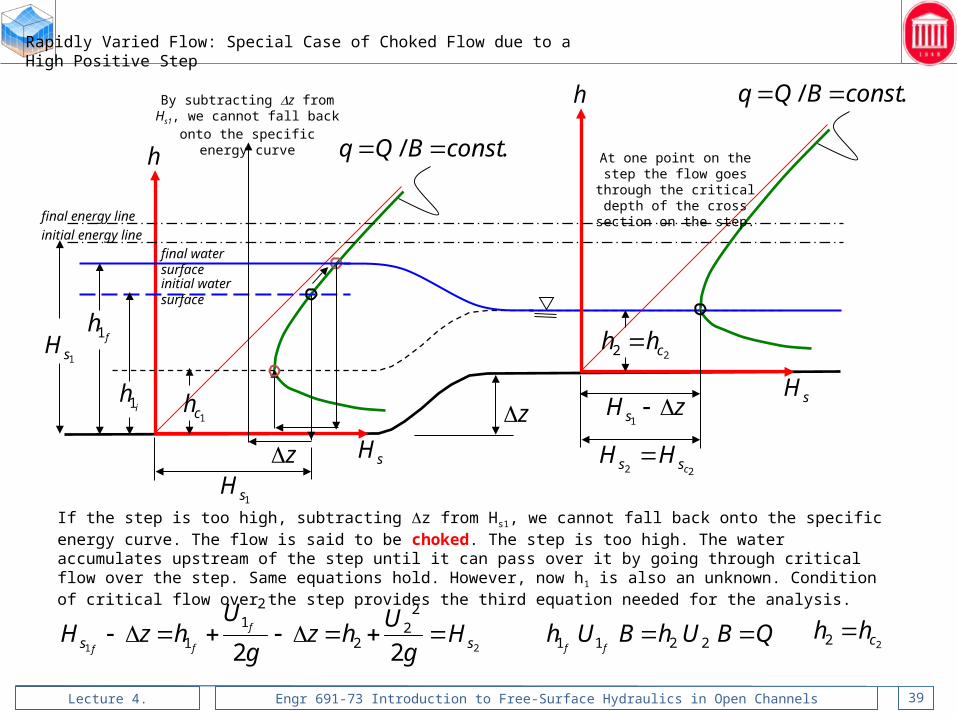
Rapidly Varied Flow: Special Case of Choked Flow due to a High Positive Step
z
1sH
z
22 chh
fh1
h
sH
zH s 1
22 css HH
h
sH
./ constBQq
./ constBQq
If the step is too high, subtracting Dz from Hs1, we cannot fall back onto the specific energy curve. The flow is said to be choked. The step is too high. The water accumulates upstream of the step until it can pass over it by going through critical flow over the step. Same equations hold. However, now h1 is also an unknown. Condition of critical flow over the step provides the third equation needed for the analysis.
QBUhBUhff
2211
1sH
21 22
22
2
21
1 ss Hg
Uhz
g
UhzH f
ff
By subtracting Dz from Hs1, we cannot fall back onto the specific
energy curve
initial water surface
final water surface
ih1
At one point on the step the flow goes through the critical depth of
the cross section on the step.
22 chh
1ch
initial energy line
final energy line

Lecture 4. Engr 691-73 Introduction to Free-Surface Hydraulics in Open Channels 40
Rapidly Varied Flow: Special Case of Choked Flow due to too much Contraction
1sH
1ch
fh1
h
sH11 / BQq
1sH
h
sH
22 / BQq
2sH
1B 2B
Top
view
Side
vie
w initial water surface
final water surface
ih1
At one point on the contracted section the flow goes through the critical depth of that cross section.
22 chh
With the available energy Hs1, we cannot cut the specific energy curve of the contracted section
22 chh
If the step is contracted too much, with the specific energy Hs1 we cannot cut the specific energy curve of the contracted section. The flow is said to be choked. The section is contracted too much. The water accumulates upstream of the contraction until it can pass a discharge of Q to the downstream by going through critical flow of the contracted section. Same equations hold. However, now h1 is also an unknown. Condition of critical flow at the contracted section provides the third equation needed for the analysis.
QBUhBUhff
221121 22
22
2
21
1 ss Hg
Uhz
g
UhzH f
ff
22 css HH
initial energy line
final energy line

Lecture 4. Engr 691-73 Introduction to Free-Surface Hydraulics in Open Channels 41
Energy Losses For Subritical Flow in Open Channel Transitions
Taken from USACE (1994)
U.S. Army Corps of Engineers, 1994. “Hydraulic Design of Flood Control Channels,” Engineering and Design Manual, EM 1110-2-1601, July 1991, Change 1 (June 1994).
Head losses at contractions and expansions can be calculated using the following expressions:
g
U
g
UCH cLc 22
21
22
g
U
g
UCH eLe 22
21
22
U1 U2 U1 U2
Contraction Expansion

Lecture 4. Engr 691-73 Introduction to Free-Surface Hydraulics in Open Channels 42
Rapidly Varied Flow: Hydraulic Jump
Hydraulic jump is a natural phenomenon that occurs when supercritical flow is forced to become subcritical.
The passage from supercritical flow to subcritical takes place with a sudden rise of the flow depth accompanied by a very turbulent motion that may entrain air into the flow.
To derive the equation governing hydraulic jump in a channel (see figure above), we will make use of momentum and continuity equations simultaneously.
12sin21
UUQFWFFF fPPx
Consider a control volume, which comprises the hydraulic jump. The upstream cross section of the control volume is in supercritical flow and the downstream section is in subcritical flow. Forces acting on this control volume are the weight of the fluid, W, the upstream and downstream pressure forces, FP1 and FP2 respectively, and the friction force, Ff. The momentum equation can be written as:
Assuming a rectangular channel, we have: BhA 11 BhA 22 BQq / 11
21A
hFP 2
1
22A
hFP
Lecture 4. Engr 691-73 Introduction to Free-Surface Hydraulics in Open Channels 43
Rapidly Varied Flow: Hydraulic Jump
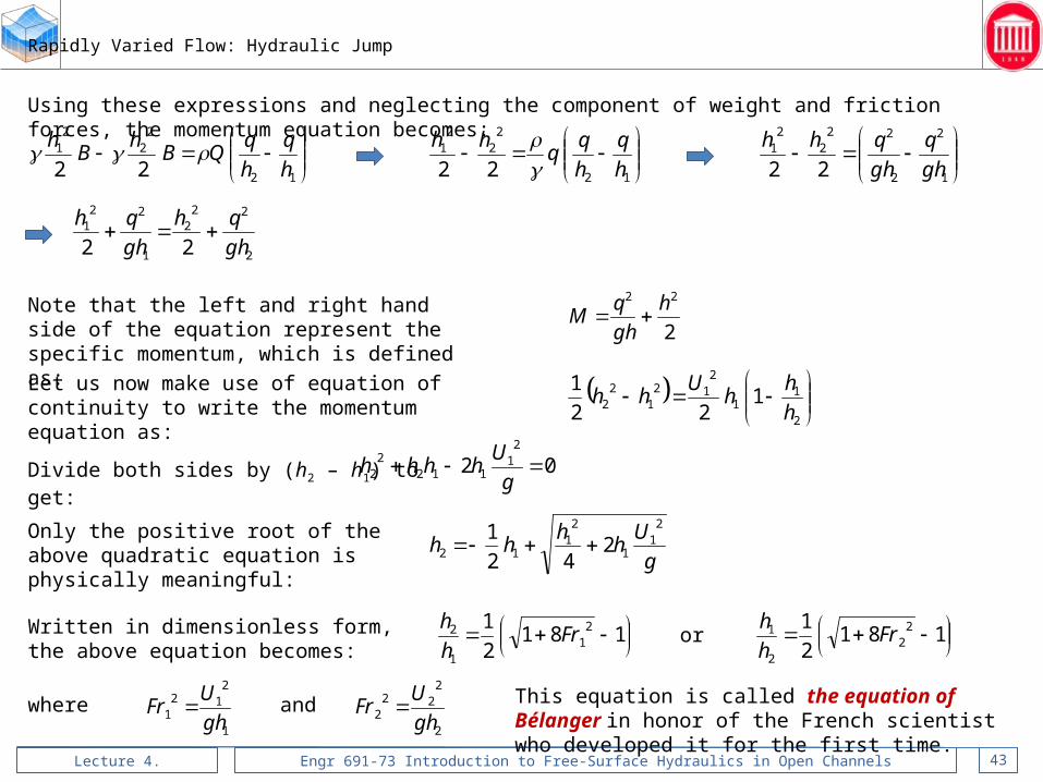
Using these expressions and neglecting the component of weight and friction forces, the momentum equation becomes:
12
22
21
22 h
q
h
qQB
hB
h
12
22
21
22 h
q
h
hh
1
2
2
222
21
22 gh
q
gh
qhh
2
222
1
221
22 gh
qh
gh
qh
Note that the left and right hand side of the equation represent the specific momentum, which is defined as: 2
22 h
gh
qM
Let us now make use of equation of continuity to write the momentum equation as:
2
11
212
12
2 122
1
h
hh
Uhh
Divide both sides by (h2 – h1) to get: 022
1112
22
g
Uhhhh
Only the positive root of the above quadratic equation is physically meaningful:
181
2
1 21
1
2 Frh
h
181
2
1 22
2
1 Frh
h
g
Uh
hhh
21
1
21
12 242
1
Written in dimensionless form, the above equation becomes:
or
where1
212
1 gh
UFr
2
222
2 gh
UFr and This equation is called the equation of Bélanger in honor
of the French scientist who developed it for the first time.

Lecture 4. Engr 691-73 Introduction to Free-Surface Hydraulics in Open Channels 44
Rapidly Varied Flow: Hydraulic Jump
Note that for a hydraulic jump on larger slopes, the weight of the fluid cannot be neglected. In this case, the equation of Bélanger for hydraulic jump becomes:
181
2
1 21
1
2 Frh
hHJ where 027.010HJ
as given by Rajaratnam.
https://www.fhwa.dot.gov/engineering/hydraulics/pubs/06086/hec14ch06.cfm#fig096
Hydraulic jumps are classified according to the approach flow Froude number.
a is in degrees

Lecture 4. Engr 691-73 Introduction to Free-Surface Hydraulics in Open Channels 45
Rapidly Varied Flow: Hydraulic Jump
21
312
22
2
21
1 42221 hh
hh
g
Uh
g
UhHHh sshj
Energy loss across the hydraulic jump:
Length of the hydraulic jump: 7512
hh
Lhj
Classification of hydraulic jumps:
7.11 Fr Undular jump
5.27.1 1 Fr Weak jump
5.45.2 1 Fr Oscillating jump
Strong jump
0.95.4 1 Fr Steady jumpjump type generally preferred in engineering applications
6.11 Fr
0.91 Fr
Photos from (Dr. H. Chanson): http://www.uq.edu.au/~e2hchans/undular.html

Lecture 4. Engr 691-73 Introduction to Free-Surface Hydraulics in Open Channels 46
Use of Hydraulic Jump in Hydraulic Engineering
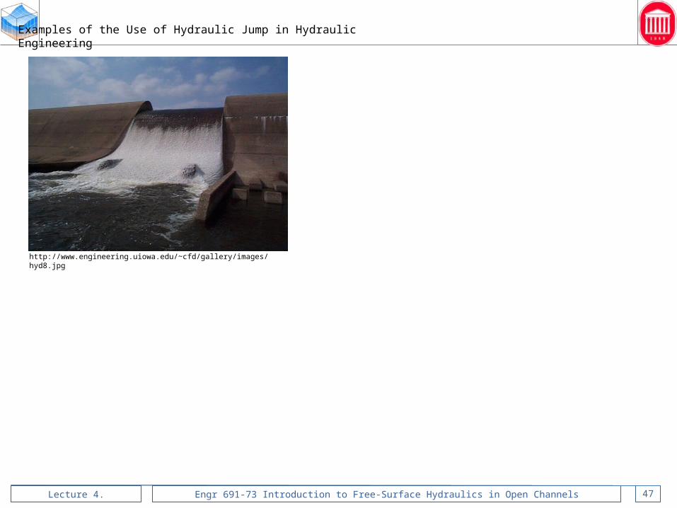
Hydraulic jump is used for dissipating the energy of high speed flow which may harm the environment if released in an uncontrolled way.
The hydraulic jump, should take place in a area where the bottom is protected (for example by a concrete slab or large size rocks). If the jump takes place on erodible material the formation of the erosion hole may endanger even the foundations of the structure.
In real engineering projects measures are taken to ensure that the hydraulic jump takes place in the area with a protected bottom. This is achieved by creating a stilling basin with the use of chute blocks, baffle piers, and end sill, etc.
Lecture 4. Engr 691-73 Introduction to Free-Surface Hydraulics in Open Channels 47
Examples of the Use of Hydraulic Jump in Hydraulic Engineering
http://www.engineering.uiowa.edu/~cfd/gallery/images/hyd8.jpg

Lecture 4. Engr 691-73 Introduction to Free-Surface Hydraulics in Open Channels 48
Design of Stilling Basins
USBR Type I Stilling Basin USBR Type II Stilling Basin
USBR Type IV Stilling Basin
USBR Type III Stilling Basin
SAF Stilling Basin Pillari’s Stilling Basin

Lecture 4. Engr 691-73 Introduction to Free-Surface Hydraulics in Open Channels 49
Books on Design of Stilling Basins
Hydraulic Design of Stilling Basins and Energy Dissipators
by A. J. Peterka, U.S. Department of the Interior,
Bureau of Reclamation
Energy Dissipators and Hydraulic Jump
by Willi H. Hager

Lecture 4. Engr 691-73 Introduction to Free-Surface Hydraulics in Open Channels 50
Positioning of a Hydraulic Jump
Draw the upstream supercritical flow profile starting from a control section at the upstream.
Draw the downstream subcritical flow profile starting from a control section at the downstream.
Draw the conjugate depth curve for the upstream supercritical flow profile.
For a hydraulic jump with zero length the jump is a vertical water surface between A’ and Z’.
If we wish to take into account the length of the jump for each point on the conjugate depth curve, draw a line parallel to the bed. The length of the line should be equal to the length of the jump, i.e. 3 to 5 times the height difference between the conjugate depth and the water depth. The tips of these lines are joined to obtain a translated conjugate depth curve which takes into account the length of the jump. The intersection of the downstream profile with the translated conjugate depth gives the downstream end of the jump.
Thus, the jump takes place between A and Z.

Lecture 4. Engr 691-73 Introduction to Free-Surface Hydraulics in Open Channels 51
Oblique Hydraulic Jump
Consider again the specific energy curve.
ss HE
gU 2/22
chh 1
gU c 2/2ch
gU 2/21
1h
ch
chh 2
Alternate depths
ss HorE
h
Specific Energy
g
UhH s 2
2
Curve plotted for a constant Q
Subcrit
ical f
low
Supercritical flow2h
It can be seen that when the flow is supercritical, a small variation in depth (say Dh) causes a large variation in kinetic energy and, thus the specific energy (DEs or DHs).
h
ss HorE
Therefore, in supercritical flow, a transition, such as a change in width or a change in direction, will provoke an abrupt variation of flow depth and stationary, stable gravity waves will appear on the free surface.
Lecture 4. Engr 691-73 Introduction to Free-Surface Hydraulics in Open Channels 52
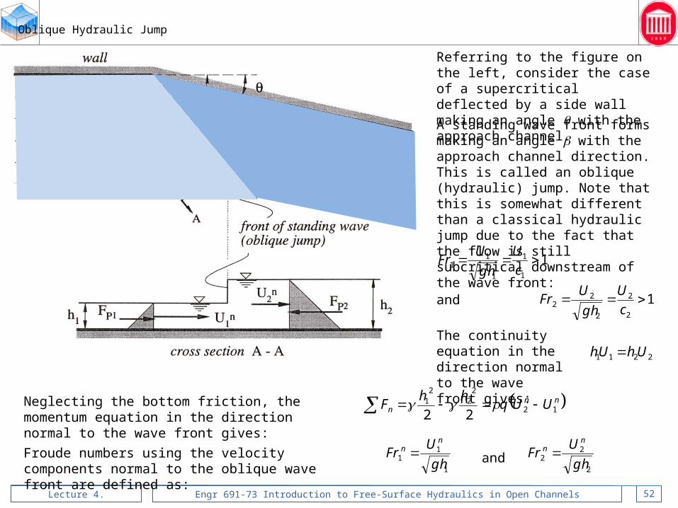
Oblique Hydraulic Jump
Referring to the figure on the left, consider the case of a supercritical deflected by a side wall making an angle q with the approach channel.
A standing wave front forms making an angle b with the approach channel direction. This is called an oblique (hydraulic) jump. Note that this is somewhat different than a classical hydraulic jump due to the fact that the flow is still subcritical downstream of the wave front:
and
11
1
1
11
c
U
gh
UFr
The continuity equation in the direction normal to the wave front gives:
2211 UhUh
Neglecting the bottom friction, the momentum equation in the direction normal to the wave front gives:
nnn UUq
hhF 12
22
21
22
Froude numbers using the velocity components normal to the oblique wave front are defined as: 1
11
gh
UFr
nn
2
22
gh
UFr
nn
12
2
2
22
c
U
gh
UFrand

Lecture 4. Engr 691-73 Introduction to Free-Surface Hydraulics in Open Channels 53
Oblique Hydraulic Jump
Note that in the direction tangent to the wave front no momentum change takes place. The equation of momentum in tangential direction becomes:
This clearly shows that:
Combining continuity and momentum equations, one obtains the equation for change of depth across an oblique jump:
In which the Froude number normal to the wave front is defined as: sin
sin1
1
1
1
11 Fr
gh
U
gh
UFr
nn
ttt UUqF 120
tt UU 21
Geometric considerations allow us to write:
sin11 UU n sin22 UU n
tan1
1
nt U
U
tan2
2
nt U
U
181
2
1 2
11
2 nFrh
h

Lecture 4. Engr 691-73 Introduction to Free-Surface Hydraulics in Open Channels 54
The angle b of the wave front can be expressed as:
Note that, for small variations of depth, thus for gradual transitions, one gets:
Combining two equations for change of depth across an oblique jump, we can write:
Using equation of continuity and geometric relationships, the equation for the oblique jump can also be written as:
tan
tan
2
1
1
2n
n
U
U
h
h
181tan2
381tantan
2
12
2
1
n
n
Fr
Fr
1
2
11sin
1
2
1
2
1 h
h
h
h
Fr
1
1
1
1sin
U
c
Fr
These derivations were originally carried out by Ippen (1949). He also experimentally verified the relationship above which gives the relationship between q and b for contracting channels (only).
Oblique Hydraulic Jump

Lecture 4. Engr 691-73 Introduction to Free-Surface Hydraulics in Open Channels 55
Oblique Hydraulic Jump
The relation ship between q and b is plotted on the left. Following observations can be made:
• For all Froude numbers there exists a maximum value for the angle of deflection, qmax.
• For all values q smaller than qmax, two values of b are possible. However, since the analysis is made for the case the flow remains supercritical after the jump, i.e. Fr2 > 1, we should consider only the values on the left side (solid lines).
It is important to note that, any perturbation created by one wall will be reflected by the other wall and so on. To study this behavior, we will consider two cases:• Asymmetrically converging channel, and• Symmetrically converging channel.
Lecture 4. Engr 691-73 Introduction to Free-Surface Hydraulics in Open Channels 56
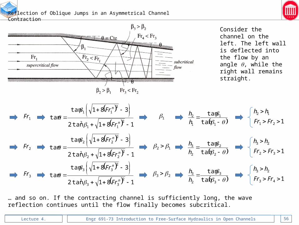
Reflection of Oblique Jumps in an Asymmetrical Channel Contraction
Consider the channel on the left. The left wall is deflected into the flow by an angle q, while the right wall remains straight.
1Fr 181tan2
381tantan
2
112
2
11
n
n
Fr
Fr
1
1
1
1
2
tan
tan
h
h 12 hh
121 FrFr
2Fr 181tan2
381tantan
2
222
2
22
n
n
Fr
Fr
12
2
2
2
3
tan
tan
h
h 23 hh
132 FrFr
3Fr 181tan2
381tantan
2
332
2
33
n
n
Fr
Fr
23
3
3
2
3
tan
tan
h
h 23 hh
143 FrFr
… and so on. If the contracting channel is sufficiently long, the wave reflection continues until the flow finally becomes subcritical.

Lecture 4. Engr 691-73 Introduction to Free-Surface Hydraulics in Open Channels 57
Reflection of Oblique Jumps in an Asymmetrical Channel Contraction
Consider the channel on the left. The left wall is deflected into the flow by an angle q, while the right wall remains straight.
1Fr 181tan2
381tantan
2
112
2
11
n
n
Fr
Fr
1
1
1
1
2
tan
tan
h
h 12 hh
121 FrFr
2Fr 181tan2
381tantan
2
222
2
22
n
n
Fr
Fr
12
2
2
2
3
tan
tan
h
h 23 hh
132 FrFr
3Fr 181tan2
381tantan
2
332
2
33
n
n
Fr
Fr
23
3
3
2
3
tan
tan
h
h 23 hh
143 FrFr
… and so on. If the contracting channel is sufficiently long, the wave reflection continues until the flow finally becomes subcritical.
Lecture 4. Engr 691-73 Introduction to Free-Surface Hydraulics in Open Channels 58
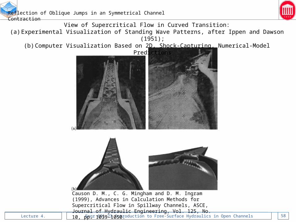
Reflection of Oblique Jumps in an Symmetrical Channel Contraction
Causon D. M., C. G. Mingham and D. M. Ingram (1999), Advances in Calculation Methods for Supercritical Flow in Spillway Channels, ASCE, Journal of Hydraulic Engineering, Vol. 125, No. 10, pp. 1039-1050.
View of Supercritical Flow in Curved Transition:(a) Experimental Visualization of Standing Wave Patterns, after Ippen and Dawson (1951);(b) Computer Visualization Based on 2D, Shock-Capturing, Numerical-Model Predictions

Lecture 4. Engr 691-73 Introduction to Free-Surface Hydraulics in Open Channels 59
Designing a Symmetrical Channel Contraction for Supercritical Flow
A good channel contraction design for supercritical flow should reduce or eliminate the undesirable cross wave pattern. This can be achieved by choosing a linear contraction length LT, thus by choosing a contraction angle q’, such that the positive waves emanating from points A and A’, due to converging walls, arrive directly at points D and D’, where negative waves are generated due to diverging walls. Such a design is shown in the figure on the left.
The choice of the angle q’ depends on the approach Froude number, Fr1, and the contraction ratio B3/B1.
Based on continuity equation, and assuming that the flow remains supercritical in the contracted section, i.e. Fr3 > 1, we can write: 3
1
2/3
3
1
33
11
1
3
Fr
Fr
h
h
Uh
Uh
B
B
From geometric considerations , we also have the relationship:tan2
31 BBLT
The angle q’ to satisfy these two equations is calculated using an iterative procedure.
Lecture 4. Engr 691-73 Introduction to Free-Surface Hydraulics in Open Channels 60
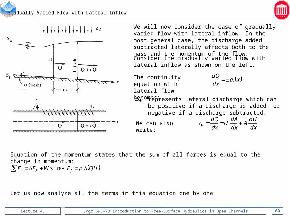
Gradually Varied Flow with Lateral Inflow
xqdx
dQ
We will now consider the case of gradually varied flow with lateral inflow. In the most general case, the discharge added subtracted laterally affects both to the mass and the momentum of the flow.
The continuity equation with lateral flow becomes:
represents lateral discharge which can be positive if a discharge is added, or negative if a discharge subtracted.
q
dx
dUA
dx
dAU
dx
dQq We can also write:
Consider the gradually varied flow with lateral inflow as shown on the left.
Equation of the momentum states that the sum of all forces is equal to the change in momentum:
QUFWFF fPx sin
Let us now analyze all the terms in this equation one by one.

Lecture 4. Engr 691-73 Introduction to Free-Surface Hydraulics in Open Channels 61
AdhAdhzAzF PPP The net hydrostatic pressure force will be:
zP is the distance from the free surface to the centroid of the flow area A:
dxASdxAW oP sinsinThe weight of the water prism between two sections that are dx apart is:
The rightmost side assumes that a is small.
dxASdxPF eof The friction force can be written as: since eho SR
The change in the momentum can be written as:
cos UdxqQUdUUdQQQU
Note that dQdxq
Note also that the lateral flow is entering or leaving the channel at an angle f and with velocity Uℓ.
Let us insert above expression the equation of momentum, and simplify:
cos UdxqQUdUUdQQdxASdxASAdh eo
A
Udxq
A
QU
A
dUUdQQdxSSdh eo
cos
Gradually Varied Flow with Lateral Inflow

Lecture 4. Engr 691-73 Introduction to Free-Surface Hydraulics in Open Channels 62
gAdx
Udxq
gAdx
QU
gAdx
dUUdQQSS
dx
dheo
cos
gA
Uq
gAdx
QUdQdUUdQQdUQU
gAdxSS
dx
dheo
cos1
gA
Uq
gAdx
QU
gAdx
UdQ
gAdx
QdU
gAdx
QUSS
dx
dheo
cos
gA
Uq
gAdx
UdQ
gAdx
QdUSS
dx
dheo
cos
gA
Uq
dx
dQ
Adx
dU
g
USS
dx
dheo
cos1
This is the equation of free surface for a steady gradually varied flow with lateral inflow, which is also called a steady spatially varied flow.
Recalling that: dQdxq and dAA
dQQdUU
Simplifying also second order terms AdA and dQdA, the spatially varied flow equation can be written as:
BgA
AQ
UgAgA
QqSS
dx
dhleo
//
1
cos1
2
2
2
It can be verified that, this equation reduces to gradually varied flow formula when lateral flow is zero, qℓ = 0.
Spatially varied flow equation can also be solved using the same methods for solving gradually varied flow equation.
Gradually Varied Flow with Lateral Inflow

Lecture 4. Engr 691-73 Introduction to Free-Surface Hydraulics in Open Channels 63
Example of Structures for Spatially Varied Flow: Side Channel Spillway
http://www.tornatore.com/joel/pics/index.php?op=dir&directory=20040227
Side channel spillway of Hoover Dam in Nevada.
http://www.firelily.com/stuff/hoover/flood.control.html
Side channel spillway of Hoover Dam in Nevada as seen from the reservoir side.

Lecture 4. Engr 691-73 Introduction to Free-Surface Hydraulics in Open Channels 64
Example of Structures for Spatially Varied Flow: Side Channel Spillway
http://www.hprcc.unl.edu/nebraska/sw-drought-2003-photos1.html
Side channel spillway of Hoover Dam in Nevada, looking downstream.

Lecture 4. Engr 691-73 Introduction to Free-Surface Hydraulics in Open Channels 65
Quiz No 1(5 minutes)
A steep channel is connected to a mild channel as shown in figure. Both channels have a rectangular cross section. The following data is given:
1nh
2nh
ch1oS
2oS
mBB 0.421
01.01oS 001.0
1oS
smnn 3/121 012.0
smQ /6 3 mhc 612.0 mhn 383.01 mhn 818.0
2
The flow in steep channel is steady and uniform. Determine in which channel, steep or mild, the hydraulic jump will take place.

Lecture 4. Engr 691-73 Introduction to Free-Surface Hydraulics in Open Channels 66
Quiz No 1(5 minutes): Solution
A steep channel is connected to a mild channel as shown in figure. Both channels have a rectangular cross section. The following data is given:
1nh
2nh
ch1oS
2oS
mBB 0.421 01.01oS 001.0
1oS
smnn 3/121 012.0 smQ /6 3
mhc 612.0 mhn 383.01 mhn 818.0
2
The flow in steep channel is steady and uniform. Determine in which channel, steep or mild, the hydraulic jump will take place.
Solution: Assume that the steady uniform flow continues all the way down to the point where the slope becomes mild. Let us see if there is a jump at that point what would be the conjugate depth.
181
2
1 21
1
1 Frh
hcj
181
2
1 2111 Frhhcj mhcj 92.0102.281383.0
2
1 21
smhB
QU
n
/91.3383.00.4
6
1
1
02.2383.081.9
91.3
1
1
ngh
UFr
mhmh ncj 818.092.0
21 A jump taking place at the point of slope change will be too strong. It can jump higher than the normal depth in the channel. Therefore, the flow continues into the mild channel without a jump and creates an M3 type profile up to a depth whose conjugate depth is equal to the uniform flow depth of the mild channel.

Lecture 4. Engr 691-73 Introduction to Free-Surface Hydraulics in Open Channels 67
Quiz No 2 (5 minutes)
Consider the channel on the left with the following data:
Determine if the flow is choked due to the positive step. What will be the flow depth over the step?
ch
ch
1h
zmh 288.01
mhc 129.0
301.01sH
193.0csH
Q
mz 12.0
Lecture 4. Engr 691-73 Introduction to Free-Surface Hydraulics in Open Channels 68
Quiz No 2 (5 minutes): Solution
Consider the channel on the left with the following data:
ch
ch
1h
zmh 288.01
mhc 129.0
301.01sH
193.0csH
Q
mz 12.0
mHmzHcss 193.0181.012.0301.0
1
Thus the flow is choked. The flow will go through the critical depth over the step, i.e. mhh c 129.02
Solution: Assuming no singular energy losses due to the step, the energy grade line remains at the same level. Over the step, the energy is reduced by an amount Dz.
Determine if the flow is choked due to the positive step. What will be the flow depth over the step?