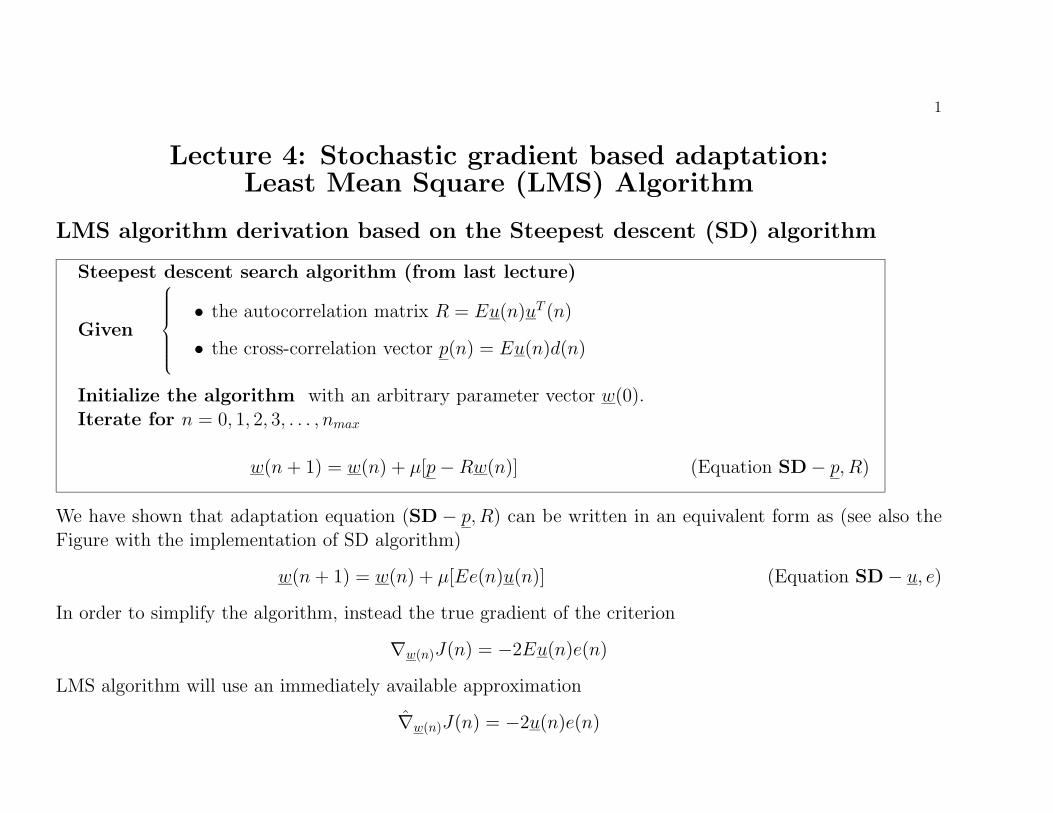
1

Lecture 4: Stochastic gradient based adaptation:Least Mean Square (LMS) Algorithm

LMS algorithm derivation based on the Steepest descent (SD) algorithm

Steepest descent search algorithm (from last lecture)

Given

⎧⎪⎪⎪⎪⎪⎨⎪⎪⎪⎪⎪⎩

• the autocorrelation matrix R = Eu(n)uT (n)

• the cross-correlation vector p(n) = Eu(n)d(n)

Initialize the algorithm with an arbitrary parameter vector w(0).Iterate for n = 0, 1, 2, 3, . . . , nmax

w(n + 1) = w(n) + µ[p − Rw(n)] (Equation SD − p, R)

We have shown that adaptation equation (SD − p, R) can be written in an equivalent form as (see also theFigure with the implementation of SD algorithm)

w(n + 1) = w(n) + µ[Ee(n)u(n)] (Equation SD − u, e)

In order to simplify the algorithm, instead the true gradient of the criterion

∇w(n)J(n) = −2Eu(n)e(n)

LMS algorithm will use an immediately available approximation

∇̂w(n)J(n) = −2u(n)e(n)

Lecture 4 2

Using the noisy gradient, the adaptation will carry on the equation

w(n + 1) = w(n) − 1

2µ∇̂w(n)J(n) = w(n) + µu(n)e(n)

In order to gain new information at each time instant about the gradient estimate, the procedure will gothrough all data set {(d(1), u(1)), (d(2), u(2)), . . .}, many times if needed.

LMS algorithm

Given

⎧⎪⎪⎪⎪⎪⎪⎪⎪⎪⎨⎪⎪⎪⎪⎪⎪⎪⎪⎪⎩

• the (correlated) input signal samples {u(1), u(2), u(3), . . .},generated randomly;

• the desired signal samples {d(1), d(2), d(3), . . .} correlatedwith {u(1), u(2), u(3), . . .}

1 Initialize the algorithm with an arbitrary parameter vector w(0), for example w(0) = 0.2 Iterate for n = 0, 1, 2, 3, . . . , nmax

2.0 Read /generate a new data pair, (u(n), d(n))2.1 (Filter output) y(n) = w(n)T u(n) =

∑M−1i=0 wi(n)u(n − i)

2.2 (Output error) e(n) = d(n) − y(n)2.3 (Parameter adaptation) w(n + 1) = w(n) + µu(n)e(n)

or componentwise

⎡⎢⎢⎢⎢⎢⎢⎢⎢⎣

w0(n + 1)w1(n + 1)

.

.

.wM−1(n + 1)

⎤⎥⎥⎥⎥⎥⎥⎥⎥⎦

=

⎡⎢⎢⎢⎢⎢⎢⎢⎢⎣

w0(n)w1(n)

.

.

.wM−1(n)

⎤⎥⎥⎥⎥⎥⎥⎥⎥⎦

+ µe(n)

⎡⎢⎢⎢⎢⎢⎢⎢⎢⎣

u(n)u(n − 1)

.

.

.u(n − M + 1)

⎤⎥⎥⎥⎥⎥⎥⎥⎥⎦

�

The complexity of the algorithm is 2M + 1 multiplications and 2M additions per iteration.

Lecture 4 3

Schematic view of LMS algorithm

Lecture 4 4

Stability analysis of LMS algorithm

SD algorithm is guaranteed to converge to Wiener optimal filter if the value of µ is selected properly (see lastLecture)

w(n) → wo

J(w(n)) → J(wo)

The iterations are deterministic : starting from a given w(0), all the iterations w(n) are perfectly determined.

LMS iterations are not deterministic: the values w(n) depend on the realization of the data d(1), . . . , d(n)and u(1), . . . , u(n). Thus, w(n) is now a random variable.

The convergence of LMS can be analyzed from following perspectives:

• Convergence of parameters w(n) in the mean:

Ew(n) → wo

• Convergence of the criterion J(w(n)) (in the mean square of the error)

J(w(n)) → J(w∞)

Assumptions (needed for mathematical tractability) = Independence theory

1. The input vectors u(1), u(2), . . . , u(n) are statistically independent vectors (very strong requirement:even white noise sequences don’t obey this property );

Lecture 4 5

2. the vector u(n) is statistically independent of all d(1), d(2), . . . , d(n − 1)

3. The desired response d(n) is dependent on u(n) but independent on d(1), . . . , d(n − 1).

4. The input vector u(n) and desired response d(n) consist of mutually Gaussian-distributed random vari-ables.

Two implications are important:

* w(n + 1) is statistically independent of d(n + 1) and u(n + 1)

* The Gaussion distribution assumption (Assumption 4) combines with the independence assumptions 1 and2 to give uncorrelated-ness statements

Eu(n)u(k)T = 0, k = 0, 1, 2, . . . , n − 1

Eu(n)d(k) = 0, k = 0, 1, 2, . . . , n − 1

Convergence of average parameter vector Ew(n)

We will subtract from the adaptation equation

w(n + 1) = w(n) + µu(n)e(n) = w(n) + µu(n)(d(n) − w(n)Tu(n))

the vector wo and we will denote ε(n) = w(n) − wo

w(n + 1) − wo = w(n) − wo + µu(n)(d(n) − w(n)Tu(n))

ε(n + 1) = ε(n) + µu(n)(d(n) − wTo u(n)) + µu(n)(u(n)Two − u(n)Tw(n))

= ε(n) + µu(n)eo(n) − µu(n)u(n)Tε(n) = (I − µu(n)u(n)T )ε(n) + µu(n)eo(n)

Lecture 4 6

Taking the expectation of ε(n + 1) using the last equality we obtain

Eε(n + 1) = E(I − µu(n)u(n)T )ε(n) + Eµu(n)eo(n)

and now using the statistical independence of u(n) and w(n), which implies the statistical independence ofu(n) and ε(n),

Eε(n + 1) = (I − µE[u(n)u(n)T ])E[ε(n)] + µE[u(n)eo(n)]

Using the principle of orthogonality which states that E[u(n)eo(n)] = 0, the last equation becomes

E[ε(n + 1)] = (I − µE[u(n)u(n)T ])E[ε(n)] = (I − µR)E[ε(n)]

Reminding the equation

c(n + 1) = (I − µR)c(n) (1)

which was used in the analysis of SD algorithm stability, and identifying now c(n) with Eε(n), we have thefollowing result:

The mean Eε(n) converges to zero, and consequently Ew(n)converges to wo

iff

0 < µ <2

λmax(STABILITY CONDITION !) where λmax is the

largest eigenvalue of the matrix R = E[u(n)u(n)T ].

Lecture 4 7

Stated in words, LMS is convergent in mean, iff the stability condition is met.

The convergence property explains the behavior of the first order characterization of ε(n) = w(n) − wo.

Now we start studying the second order characterization of ε(n).

ε(n + 1) = ε(n) + µu(n)e(n) = ε(n) − 1

2µ∇̂J(n)

Now we split ∇̂J(n) in two terms: ∇̂J(n) = ∇J(n) + 2N(n) where N(n) is the gradient noise. ObviouslyE[N(n)] = 0

u(n)e(n) = −1

2∇̂J(n) = −1

2∇J(n) − N(n) = −(Rw(n) − p) − N(n)

= −R(w(n) − wo) − N(n) = −Rε(n) − N(n)

ε(n + 1) = ε(n) + µu(n)e(n) = ε(n) − µRε(n) − µN(n)

= (I − µR)ε(n) − µN(n) = (I − QΛQH)ε(n) − µN(n) = Q(I − µΛ)QHε(n) − µN(n)

We denote ε′(n) = QHε(n) and N ′(n) = QHN(n) the rotated vectors (remember, Q is the matrix formed bythe eigenvectors of matrix R) and we thus obtain

ε′(n + 1) = (I − µΛ)ε′(n) − µN ′(n)

or written componentwise

ε′j(n + 1) = (1 − µλj)ε′j(n) − µN ′

j(n)

Lecture 4 8

Taking the modulus and then taking the expectation in both members:

E|ε′j(n + 1)|2 = (1 − µλj)2E|ε′j(n)|2 − 2µ(1 − µλj)E[N ′

j(n)ε′j(n)] + µ2E[|N ′j(n)|]2

Making the assumption: E[N ′j(n)ε′j(n)] = 0 and denoting

γj(n) = E[|ε′j(n)|]2

we obtain the recursion showing how γj(n) propagates through time.

γj(n + 1) = (1 − µλj)2γj(n) + µ2E[|N ′

j(n)|]2

More information can be obtained if we assume that the algorithm is in the steady-state, and therefore ∇J(n)is close to 0. Then

e(n)u(n) = −N(n)

i.e. the adaptation vector used in LMS is only noise. Then

E[N(n)N(n)T ] = E[e2(n)u(n)u(n)T ] ≈ E[e2(n)]E[u(n)u(n)T ] = JoR = JoQΛQH

and therefore

E[N ′(n)N ′(n)H ] = JoΛ

or componentwise

E[|N ′j(n)|]2 = Joλj

and finally

γj(n + 1) = (1 − µλj)2γj(n) + µ2Joλj

Lecture 4 9

We can iterate this to obtain

γj(n + 1) = (1 − µλj)2nγj(0) + µ2

n/2∑

i=0(1 − µλj)

2iJoλj

Using the assumption |1 − µλj| < 1(which is also required for convergence in mean) at the limit

limn→∞ γj(n) = µ2Joλj

1

1 − (1 − µλj)2 =µJo

2 − µλj

This relation gives an estimate of the variance of the elements of QH(w(n) − wo) vector. Since this varianceconverges to a nonzero value, it results that the parameter vector w(n) continues to fluctuate around theoptimal vector wo. In Lecture 2 we obtained the canonical form of the quadratic form which expresses themean square error:

J(n) = Jo +M∑

i=1λi|νi|2

where ν was defined asν(n) = QHc(n) = QH(w(n) − wo) (2)

Similarly it can be shown that in the case of LMS adaptation, and using the independence assumption,

J(n) = Jo +M∑

i=1λiE|ε′i|2 = Jo +

M∑

i=1λiγi(n)

Lecture 4 10

and defining the criterion J∞ as the value of criterion J(w(n)) = J(n) when n → ∞ we obtain

J∞ = Jo +M∑

i=1λi

µJo

2 − µλi

For µλi � 2

J∞ = Jo + µJo

M∑

i=1λi/2 = Jo(1 + µ

M∑

i=1λi/2) = Jo(1 + µtr(R)/2) = (3)

J∞ = Jo(1 + µMr(0)/2) = Jo(1 +µM

2· Power of the input) (4)

The steady state mean square error J∞ is close to optimal mean square error if µ is small enough.

In [Haykin 1991] there was a more complex analysis, involving the transient analysis of J(n). It showed thatconvergence in mean square sense can be obtained if

M∑

i=1

µλi

2(1 − µλi)< 1

or in another, simplified, form

µ <2

Power of the input

Lecture 4 11

Small Step Size Statistical Theory (Haykin 2002)

• Assumption 1 The step size parameter µ is small, so the LMS acts as a low pass filter with a low cutofffrequency.

It allows to approximate the equation

ε(n + 1) = (I − µu(n)u(n)T )ε(n) − µu(n)eo(n) (5)

by an approximation:

εo(n + 1) = (I − µR)εo(n) − µu(n)eo(n) (6)

• Assumption 2 The physical mecanism for generating the desired response d(n) has the same form asthe adaptive filter d(n) = wT

o u(n) + eo(n) where eo(n) is a white noise, statistically independent of u(n).

• Assumption 3 The input vector u(n) and the desired response d(n) are jointly Gaussian.

Lecture 4 12

Learning curves

The statistical performance of adaptive filters is studied using learning curves, averaged over many realizations,or ensemble-averaged.

• The mean square error MSE learning curve Take an ensemble average of the squared estimationerror e(n)2

J(n) = Ee2(n) (7)

• The mean-square deviation (MSD) learning curve Take an ensemble average of the squared errordeviation ||ε(n)||2

D(n) = E||ε(n)||2 (8)

• The excess mean-square-error

Jex(n) = J(n) − Jmin (9)

where Jmin is the MSE error of the optimal Wiener filter.

Lecture 4 13

Results of the small step size theory

The statistical performance of adaptive filters is studied using learning curves, averaged over many realizations,or ensemble-averaged.

• Connection between MSE and MSD

λminD(n) ≤ Jex(n) ≤ λmaxD(n) (10)

Jex(n)/λmin ≤ D(n) ≤ Jex(n)/λmax (11)

It is therefore enough to study the transient behavior of Jex(n), since D(n) follows its evolutions.

• The condition for stability

0 < µ <2

λmax(12)

• The excess mean-square-error converges to

Jex(∞) =µJmin

2

M∑

k=1λk (13)

• The misadjustment

M =Jex(∞)

Jmin=

µ

2

M∑

k=1λk =

µ

2tr(R) =

µ

2Mr(0) (14)

Lecture 4 14

Application of LMS algorithm : Adaptive Equalization

Lecture 4 15

Modelling the communication channel

We assume the impulse response of the channel in the form

h(n) =

⎧⎨⎩

12

[1 + cos(2π

W (n − 2))], n = 1, 2, 3

0, otherwise

The filter input signal will be

u(n) = (h ∗ a)(n) =3∑

k=1h(k)a(n − k) + v(n)

where σ2v = 0.001

Selecting the filter structure

The filter has M = 11 delays units (taps).

The weights (parameter) of the filter are symmetric with respect to the middle tap (n = 5).

The channel input is delayed 7 units to provide the desired response to the equalizer.

Correlation matrix of the Equalizer input

Since u(n) =∑3

k=1 h(k)a(n − k) + v(n) is a MA process, the correlation function will be

r(0) = h(1)2 + h(2)2 + h(3)2 + σ2v

r(1) = h(1)h(2) + h(2)h(3)

r(2) = h(1)h(3)

r(3) = r(4) = . . . = 0

Lecture 4 16

0 2 4 6 8 100

0.2

0.4

0.6

0.8

1Channel input response h(n)

0 20 40 60−1.5

−1

−0.5

0

0.5

1

1.5Convolved (distorted) signal h*a

0 20 40 60−1

−0.5

0

0.5

1Original signal to be transmitted a(n)

0 20 40 60−1.5

−1

−0.5

0

0.5

1

1.5Received signal u(n)(noise + distorted)

Sample signals in adaptive equalizer experiment

Lecture 4 17

Effect of the parameter W on the eigenvalue spread

We define the eigenvalue spread χ(R) of a matrix as the ratio of the maximum eigenvalue over the minimumeigenvalue

W 2.9 3.1 3.3 3.5

r(0) 1.0973 1.1576 1.2274 1.3032

r(1) 0.4388 0.5596 0.6729 0.7775

r(2) 0.0481 0.0783 0.1132 0.1511

λmin 0.3339 0.2136 0.1256 0.0656

λmax 2.0295 2.3761 2.7263 3.0707

χ(R) = λmax/λmin 6.0782 11.1238 21.7132 46.8216

Lecture 4 18

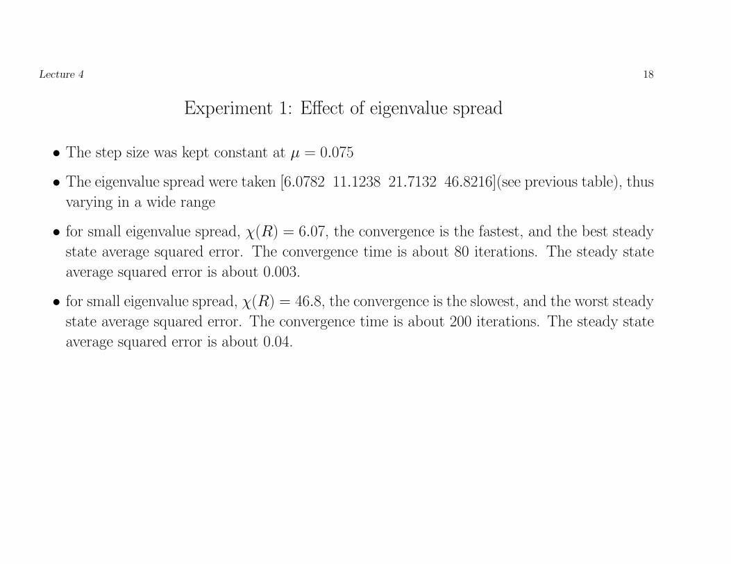
Experiment 1: Effect of eigenvalue spread

• The step size was kept constant at µ = 0.075

• The eigenvalue spread were taken [6.0782 11.1238 21.7132 46.8216](see previous table), thus

varying in a wide range

• for small eigenvalue spread, χ(R) = 6.07, the convergence is the fastest, and the best steady

state average squared error. The convergence time is about 80 iterations. The steady state

average squared error is about 0.003.

• for small eigenvalue spread, χ(R) = 46.8, the convergence is the slowest, and the worst steady

state average squared error. The convergence time is about 200 iterations. The steady state

average squared error is about 0.04.

Lecture 4 19

Learning curves for µ = 0.075, W = [2.9 3.1 3.3 3.5]

0 50 100 150 200 250 300 350 400 450 50010

−3

10−2

10−1

100

101

102

103

Learning curve Ee2(n) for LMS algorithm

time step n

W=2.9W=3.1W=3.3W=3.5

Lecture 4 20

Experiment 2: Effect of step size

• The eigenvalue spread was kept constant at χ = 11.12

• The step size were taken [0.0075 0.025 0.075], thus varying in a range1:10

• for smallest step sizes, µ = 0.0075, the convergence is the slowest, and the best steady state

average squared error. The convergence time is about 2300 iterations. The steady state

average squared error is about 0.001.

• for large step size, µ = 0.075, the convergence is the fastest, and the worst steady state average

squared error. The convergence time is about 100 iterations. The steady state average squared

error is about 0.005.

Lecture 4 21

Learning curves for µ = [0.0075 0.025 0.075]; W = 3.1

0 500 1000 1500 2000 2500 300010

−3

10−2

10−1

100

101

Learning curve Ee2(n) for LMS algorithm

time step n

µ=0.0075µ=0.025 µ=0.075

Lecture 4 22

% Adaptive equalization

% Simulate some (useful) signal to be transmitted

a= (randn(500,1)>0) *2-1; % Random bipolar (-1,1) sequence;

% CHANNEL MODEL

W=2.9;

h= [ 0, 0.5 * (1+cos(2*pi/W*(-1:1))) ];

ah=conv(h,a);

v= sqrt(0.001)*randn(500,1); % Gaussian noise with variance 0.001;

u=ah(1:500)+v;

subplot(221) , stem(impz(h,1,10)), title(’Channel input response h(n)’)

subplot(222) , stem(ah(1:59)), title(’Convolved (distorted) signal h*a’)

subplot(223) , stem(a(1:59)), title(’Original signal to be transmitted’)

subplot(224) , stem(u(1:59)), title(’Received signal (noise + distortion)’)

% Deterministic design of equalizer (known h(n))

Lecture 4 23

H=diag(h(1)*ones(9,1),0) +diag(h(2)*ones(8,1),-1) + diag(h(3)*ones(7,1),-2);

H=[H ; zeros(1,7) h(2) h(3); zeros(1,8) h(3) ]

b=zeros(11,1); b(6)=1;

c=H\b

% Independent trials N=200

average_J= zeros(500,1);N=2

for trial=1:N

v= sqrt(0.001)*randn(500,1); % Gaussian noise with variance 0.001;

u=ah(1:500)+v;

% Statistical design of equalizer (unkown h(n))

mu= 0.075;

w=zeros(11,1);

for i=12:500

y(i)=w’*u((i-11):(i-1));

e(i)=a(i-7)-y(i);

w=w+mu*e(i)*u((i-11):(i-1));

J(i)=e(i)^2;

Lecture 4 24

average_J(i)=average_J(i)+J(i);

end

end

average_J=average_J/N;

semilogy(average_J), title(’Learning curve Ee^2(n) for LMS algorithm’),

xlabel(’time step n’)

Lecture 4 25

Summary

• LMS is simple to implement.

• LMS does not require preliminary modelling.

• Main disadvantage: slow rate of convergence.

• Convergence speed is affected by two factors: the step size and the eigenvalue spread of the

correlation matrix.

• The condition for stability is

0 < µ <2

λmax

• For LMS filters with filter length M moderate to large, the convergence condition on the step

size is

0 < µ <2

MSmax

where Smax is the maximum value of the power spectral density of the tap inputs.