CHAPTER 2I. GENERAL SERVICE SIGNS Section 2I.01 Sizes of General

Randomized Algorithms
Textbook:
Randomized Algorithms, by Rajeev Motwani and Prabhakar Raghavan.
1
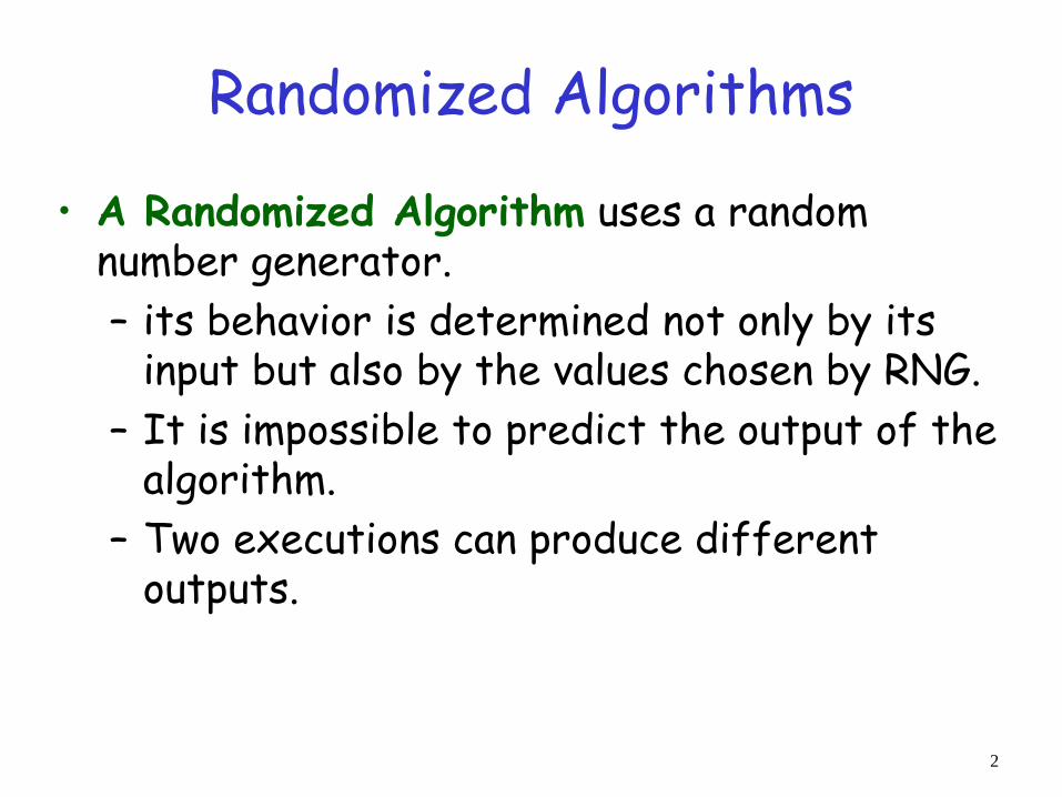
Randomized Algorithms
• A Randomized Algorithm uses a random number generator.
– its behavior is determined not only by its input but also by the values chosen by RNG.
– It is impossible to predict the output of the algorithm.
– Two executions can produce different outputs.
2

Why Randomized Algorithms?
• Efficiency • Simplicity • Reduction of the impact of bad cases! • Fighting an adversary.
3

Types of Randomized Algorithms
• Las Vegas algorithms – Answers are always correct,
running time is random
– In analysis: bound expected running time
• Monte Carlo algorithms – Running time is fixed,
answers may be incorrect
– In analysis: bound error probabilities
4
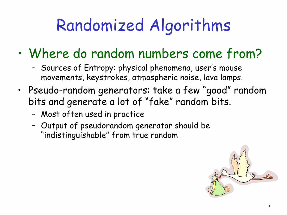
Randomized Algorithms
• Where do random numbers come from? – Sources of Entropy: physical phenomena, user’s mouse
movements, keystrokes, atmospheric noise, lava lamps.
• Pseudo-random generators: take a few “good” random bits and generate a lot of “fake” random bits. – Most often used in practice
– Output of pseudorandom generator should be “indistinguishable” from true random
5

We will see (up to random decisions):
1. A randomized approximation Algorithm for determining the value of .
2. A Randomized algorithm for the selection problem.
3. A randomized data structure. 4. Analysis of random walk on a graph. 5. A randomized graph algorithm.
6 6
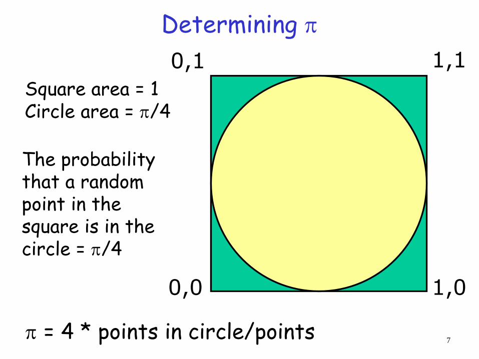
Determining
0,1 1,1
1,0 0,0
Square area = 1 Circle area = /4
The probability that a random point in the square is in the circle = /4
= 4 * points in circle/points 7

Determining def findPi (points): incircle = 0 for i in 1 to points: x = random() // float in [0,1] y = random() if (x - ½)2 + (y - ½)2 < 0.25)
incircle = incircle + 1 return 4.0 * incircle / points
Note : a point is in the circle if its distance from (½, ½) < r 8

Determining - Results
1 0.0 2 4.0 4 3.0 64 3.0625 1024 3.1640625 16384 3.1279296 131072 3.1376647 1048576 3.1411247
If we wait long enough will it produce an arbitrarily accurate value?
n Output Real = 3.14159265
9

Basic Probability Theory (a short recap)
• Sample Space Ω: – Set of possible outcome points
• Event AΩ: – A subset of outcomes
• Pr[A]: probability of an event – For every event A: Pr[A][0,1]
– If AB= then Pr[AB]=Pr[A]+Pr[B]
– Pr[Ω]=1
Sample space
0.1 0.1
0.1
0.3
0.2
0.05
0.1
0.05 0
0.35
10
Basic Probability Theory (a short recap)
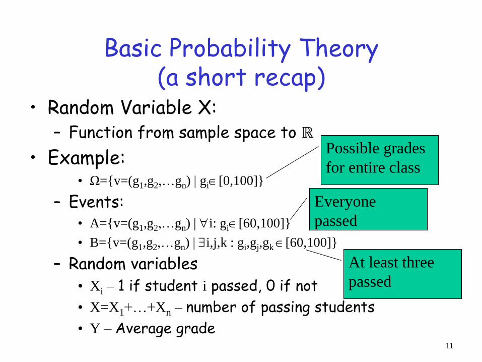
• Random Variable X: – Function from sample space to ℝ
• Example: • Ω=v=(g1,g2,…gn) | gi[0,100]
– Events: • A=v=(g1,g2,…gn) | i: gi[60,100]
• B=v=(g1,g2,…gn) | i,j,k : gi,gj,gk [60,100]
– Random variables
• Xi – 1 if student i passed, 0 if not
• X=X1+…+Xn – number of passing students
• Y – Average grade
Possible grades
for entire class
Everyone
passed
At least three
passed
11

Basic Probability Theory (a short recap)
• Expectation of a Random Variable X: – E[X]=xxPr[X=x] – the “average value”
• Expectation of Indicator Variables: – E[Xi]=Pr[Xi=1] – for an indicator r.v.
• Linearity of Expectation: – E[a1X1+…+anXn]=a1E[X1]+…+anE[Xn]
– Works for arbitrary random variables!
12
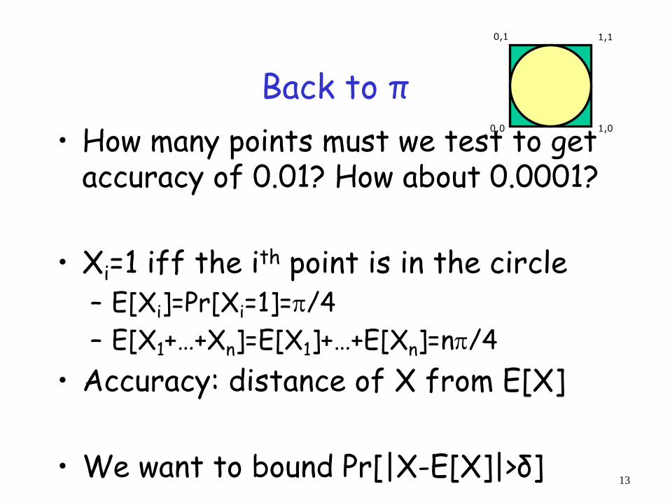
Back to π
• How many points must we test to get accuracy of 0.01? How about 0.0001?
• Xi=1 iff the ith point is in the circle – E[Xi]=Pr[Xi=1]=/4
– E[X1+…+Xn]=E[X1]+…+E[Xn]=n/4
• Accuracy: distance of X from E[X]
• We want to bound Pr[|X-E[X]|>δ]
0,1 1,1
1,0 0,0
13
A Simple Calculation
If the average income of people is $100 then more than 50% of the people can be
earning more than $200 each
False! else the average would be higher!!!
True or False:
14
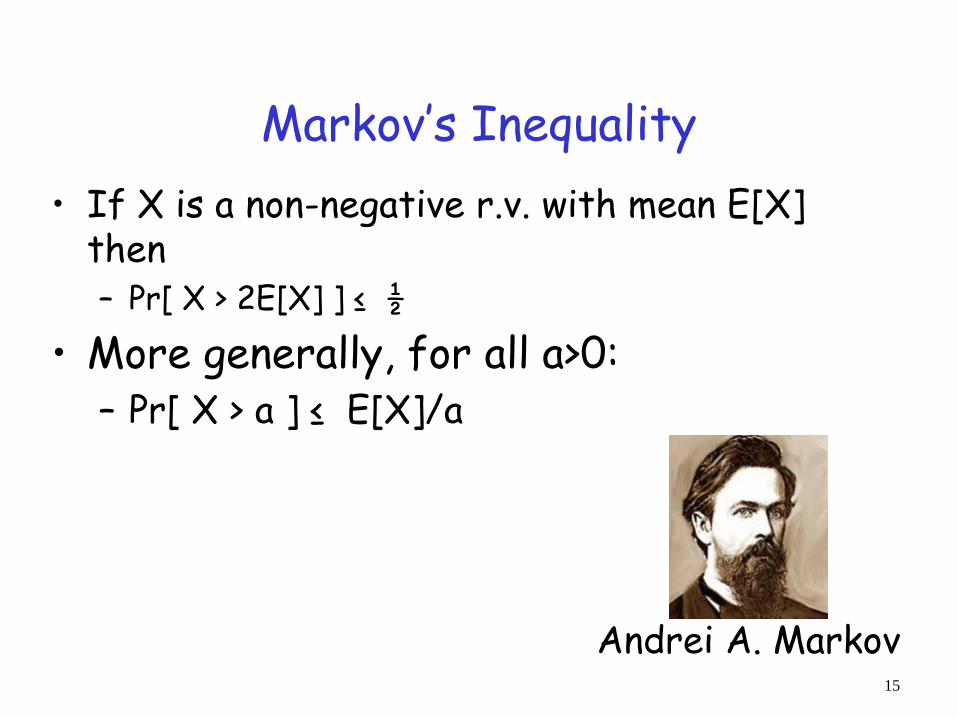
Andrei A. Markov
Markov’s Inequality
• If X is a non-negative r.v. with mean E[X] then – Pr[ X > 2E[X] ] ≤ ½
• More generally, for all a>0: – Pr[ X > a ] ≤ E[X]/a
15

(since X,a non-neg)
Markov’s Inequality
Non-neg random variable X has expectation E[X]
E[X] = 𝑥 ∙ Pr 𝑋 = 𝑥𝑥
≥ 𝑥 ∙ Pr 𝑋 = 𝑥𝑥≥𝑎
≥ 𝑎 ∙ Pr 𝑋 = 𝑥𝑥≥𝑎
= 𝑎 Pr 𝑋 = 𝑥𝑥≥𝑎
= 𝑎 Pr 𝑋 ≥ 𝑎
Pr 𝑋 ≥ 𝑎 ≤ E X /𝑎
16

Back to π again
• X is the number of points in the circle – X is non-negative
– E[X]=n/4
• What does Markov’s inequality give us?
– Pr 𝑋 − 𝐸 𝑋 > 𝛿 = Pr 𝑋 > 𝛿 + 𝐸 𝑋 ≤𝐸[𝑋]
𝐸 𝑋 +𝛿
– However, 𝐸[𝑋]
𝐸 𝑋 +𝛿→ 1 when 𝑛 → ∞
• Not good enough!
0,1 1,1
1,0 0,0
17

Chernoff-Hoeffding Bound
• Used to bound convergence of sums of
random variables: X=X1+…+Xn
– Xi are zero/one variables
– All variables are independent
• For all i,j: Pr[Xi=1|Xj=1]=Pr[Xi=1]
– Denote 𝜇 = 𝐸 𝑋 /𝑛
• When satisfied, sum converges
exponentially fast !
Pr𝑋
𝑛− 𝜇 ≥ 𝛿𝜇 ≤ 2𝑒−
𝑛𝛿2𝜇3
18
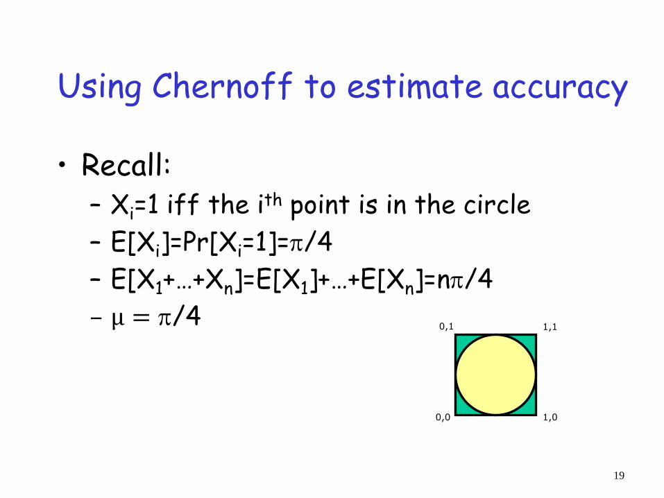
Using Chernoff to estimate accuracy
• Recall: – Xi=1 iff the ith point is in the circle
– E[Xi]=Pr[Xi=1]=/4
– E[X1+…+Xn]=E[X1]+…+E[Xn]=n/4
– µ = /4 0,1 1,1
1,0 0,0
19

Using Chernoff to estimate accuracy
• Using Chernoff:
Pr𝑋
𝑛− 𝜇 ≥ 𝛿𝜇 ≤2𝑒−
𝑛𝛿2𝜇3 ⇔ Pr
𝑋
𝑛− 𝜇 ≥ 𝛿 ≤2𝑒
−𝑛𝛿2
3𝜇
• To get close within 𝛿 with error prob. 𝜖:
2𝑒−𝑛𝛿2
3𝜇 < 𝜖 ⇔ 𝑛 >3𝜇 ln 2/𝜖
𝛿2=3𝜋 ln 2/𝜖
4𝛿2
• E.g.: to get 0.01 accuracy with 95% success:
𝜖 = 0.05, 𝛿 = 0.01 ⇒ 𝑛 >3𝜋 ln 40
4 ⋅ 0.0001≈ 86917
20
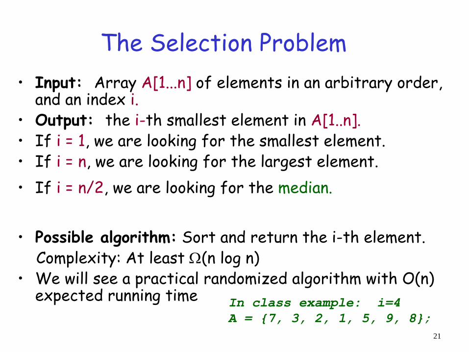
The Selection Problem
• Input: Array A[1...n] of elements in an arbitrary order, and an index i.
• Output: the i-th smallest element in A[1..n]. • If i = 1, we are looking for the smallest element. • If i = n, we are looking for the largest element.
• If i = n/2, we are looking for the median.
• Possible algorithm: Sort and return the i-th element. Complexity: At least (n log n) • We will see a practical randomized algorithm with O(n)
expected running time
21
In class example: i=4
A = 7, 3, 2, 1, 5, 9, 8;

Randomized Selection
• Key idea: similar to quicksort
• Choose a random element q
• partition the array into small (<q) and big (>q) elements.
• Keep searching in the appropriate side.
<q >q q
22

Randomized Selection
Select(A,i)
• If array A is of size 1 – trivial
• Randomly partition A with pivot q.
• Suppose q was the k’th smallest element
• If i=k, answer is q
• If i<k, recursively select i’th element in left subarray
• If i>k, recursively find (i-k)’th element in right subarray
<q >q q
23 k
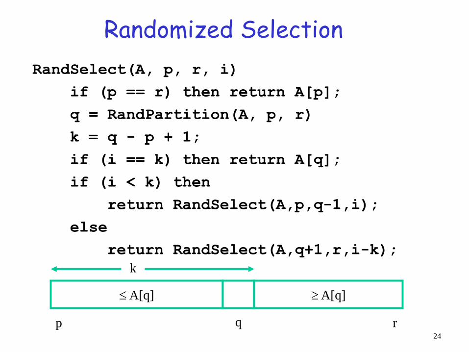
Randomized Selection
RandSelect(A, p, r, i)
if (p == r) then return A[p];
q = RandPartition(A, p, r)
k = q - p + 1;
if (i == k) then return A[q];
if (i < k) then
return RandSelect(A,p,q-1,i);
else
return RandSelect(A,q+1,r,i-k);
A[q] A[q]
k
q p r 24

How to partition?
We choose a random element q and want to move all elements smaller than q before q. and all elements greater than q after q.
• Keep two indices, one running from left and the other from right.
• Move each index until points to an element that belongs to the other side
• swap the two elements and repeat.
• Stop when indices cross each other.
Running time?
25
O(n)
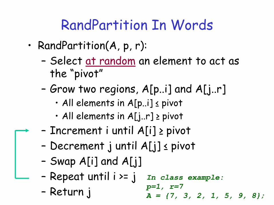
RandPartition In Words
• RandPartition(A, p, r):
– Select at random an element to act as the “pivot”
– Grow two regions, A[p..i] and A[j..r] • All elements in A[p..i] ≤ pivot
• All elements in A[j..r] ≥ pivot
– Increment i until A[i] ≥ pivot
– Decrement j until A[j] ≤ pivot
– Swap A[i] and A[j]
– Repeat until i >= j
– Return j
In class example:
p=1, r=7
A = 7, 3, 2, 1, 5, 9, 8;
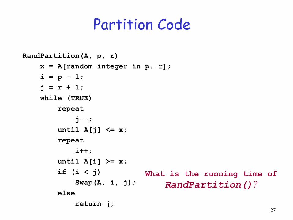
Partition Code
RandPartition(A, p, r)
x = A[random integer in p..r];
i = p - 1;
j = r + 1;
while (TRUE)
repeat
j--;
until A[j] <= x;
repeat
i++;
until A[i] >= x;
if (i < j)
Swap(A, i, j);
else
return j;
What is the running time of
RandPartition()?
27

Randomized Selection
• Analysis: – Worst case: partition always 0:n-1
T(n) = T(n-1) + O(n)
= O(n2) (arithmetic series)
• Worse than sorting!
– “Best” case: suppose an n : (1-)n partition for some fraction . T(n) = T(n) + O(n)
= O(n) (Master Theorem, case 3)
• Better than sorting!
a=1, b=1/
f(n)=Ω(nlogb(a)+ε)
28
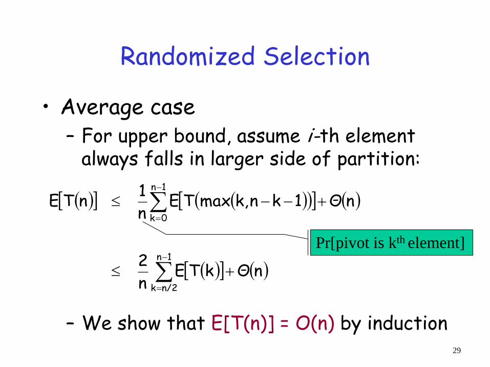
Randomized Selection
• Average case – For upper bound, assume i-th element
always falls in larger side of partition:
– We show that E[T(n)] = O(n) by induction
1n
n/2k
1n
0k
nΘkTEn
2
nΘ1knk,maxTEn
1nTE
Pr[pivot is kth element]
29
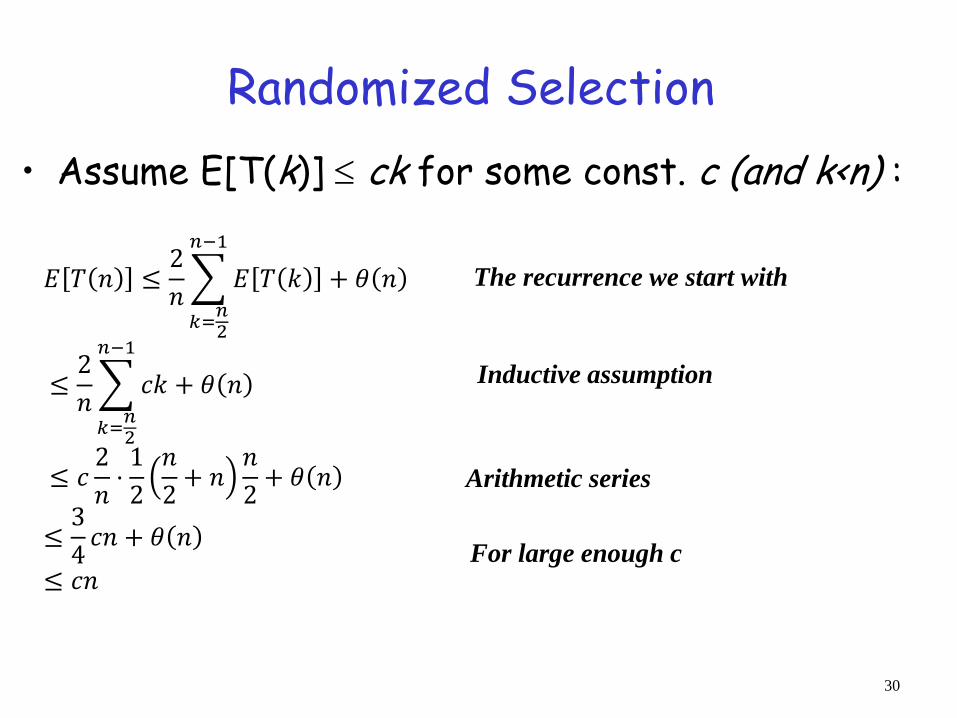
Randomized Selection
• Assume E[T(k)] ck for some const. c (and k<n) :
The recurrence we start with
Inductive assumption
Arithmetic series
For large enough c
30
𝐸 𝑇 𝑛 ≤2
𝑛 𝐸 𝑇 𝑘
𝑛−1
𝑘=𝑛2
+ 𝜃 𝑛
≤2
𝑛 𝑐𝑘
𝑛−1
𝑘=𝑛2
+ 𝜃 𝑛
≤ 𝑐2
𝑛⋅1
2
𝑛
2+ 𝑛𝑛
2+ 𝜃 𝑛
≤3
4𝑐𝑛 + 𝜃 𝑛
≤ 𝑐𝑛

Randomized Selection
• We got a randomized selectio algorithm that runs in expected linear time.
• Is this Monte Carlo or Las vegas?
31

Skip lists – a randomized data structure
Review: • Sorted Linked List
What is the worst case performance of find( ), insert( )?
• Sorted Array What is the worst case performance of find( ),
insert( )?
3 9 12 18 29 35 37
3 9 12 18 29 35 37 32

An Alternative Sorted Linked List
• What if you skip every other node?
– Every other node has a pointer to the next and the one after that
• Find :
– follow “skip” pointer until pass target
• Resources
– Additional storage
• Performance of find( )?
33

Skipping every 2nd node
The value stored in each node is shown below the node and corresponds to the the position of the node in the list.
It’s clear that find( ) does not need to examine every node. It can skip over every other node, then do a final examination at the end. The number of nodes examined is no more than n/2 + 1.
For example the nodes examined finding the value 15 would be 2, 4, 6, 8, 10, 12, 14, 16, 15 -- a total of 16/2 + 1 = 9.
34

Skipping every 2nd and 4th node
The find operation can now make bigger skips than the previous example. Every 4th node is skipped until the search is confined between two nodes. At this point as many as three nodes may need to be scanned. The number of nodes examined is no more than n / 4 + 3.
Again, look at the nodes examined when searching for 15
35

Skipping every 2i-th node
Add hierarchy of skip pointers every 2i-th node points 2i nodes ahead For example, every 2nd node has a reference 2 nodes ahead; every 8th node has a reference 8 nodes ahead
We can now search just as binary search in an array.
The max number of nodes examined is O(log n). 36

Some serious problems
• what happens when we insert or remove a value from the list? Reorganizing the list is θ(n).
• E.g., removing the first element in the list elements that were in odd positions (only at lowest level) are now at even positions and vice versa.
37

A Probabilistic Skip Lists
• Concept: A skip list that maintains the same distribution of nodes, but without the requirement for the rigid pattern of node sizes
• On average, 1/2 have 1 pointer
• On average, 1/4 have 2 pointers
• …
• On average, 1/2i have i pointers
• It’s no longer necessary to maintain the rigid pattern by moving values around for insert and remove. This gives us a high probability of still having O(log n) performance. The probability that a skip list will behave badly is very small.
38

A Probabilistic Skip List
The number of forward reference pointers a node has is its “size”
The distribution of node sizes is exactly the same as the previous figure, the nodes just occur in a different pattern.
39
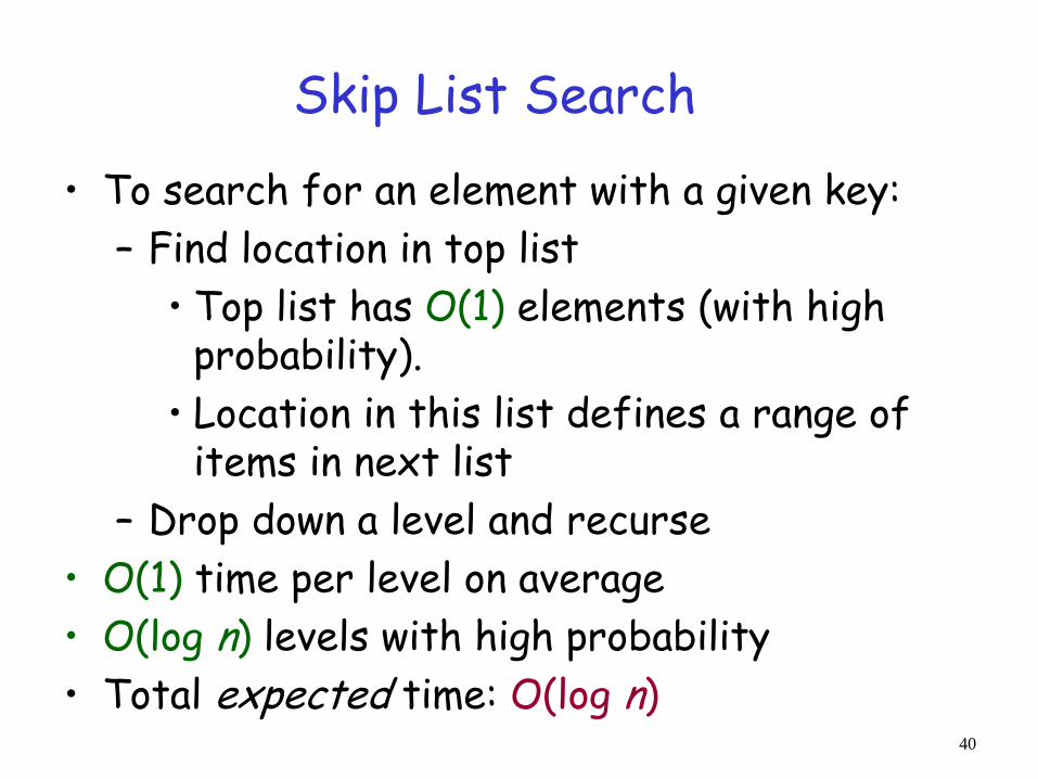
Skip List Search
• To search for an element with a given key:
– Find location in top list
• Top list has O(1) elements (with high probability).
• Location in this list defines a range of items in next list
– Drop down a level and recurse
• O(1) time per level on average
• O(log n) levels with high probability
• Total expected time: O(log n) 40

Skip List Insert
1. Perform a search for that key
2. Insert element in bottom-level list
3. With probability p, recurse to insert in upper level (note: p does not have to be 1/2)
– Expected number of occurances = 1+ p + p2 + … = = 1/(1-p) = O(1) if p is constant
– Total time = Search + O(1) = O(log n) expected
Skip list delete: O(1) (assuming a pointer to the element is given)
41
Probabilistic Skip Lists - summary
• O(log n) expected time for find, insert
• O(n) time worst case (Why?) – But random, and probability of getting worst-
case behavior is extremely small
• O(n) expected storage requirements (Why?)
• Easy to code
42
-
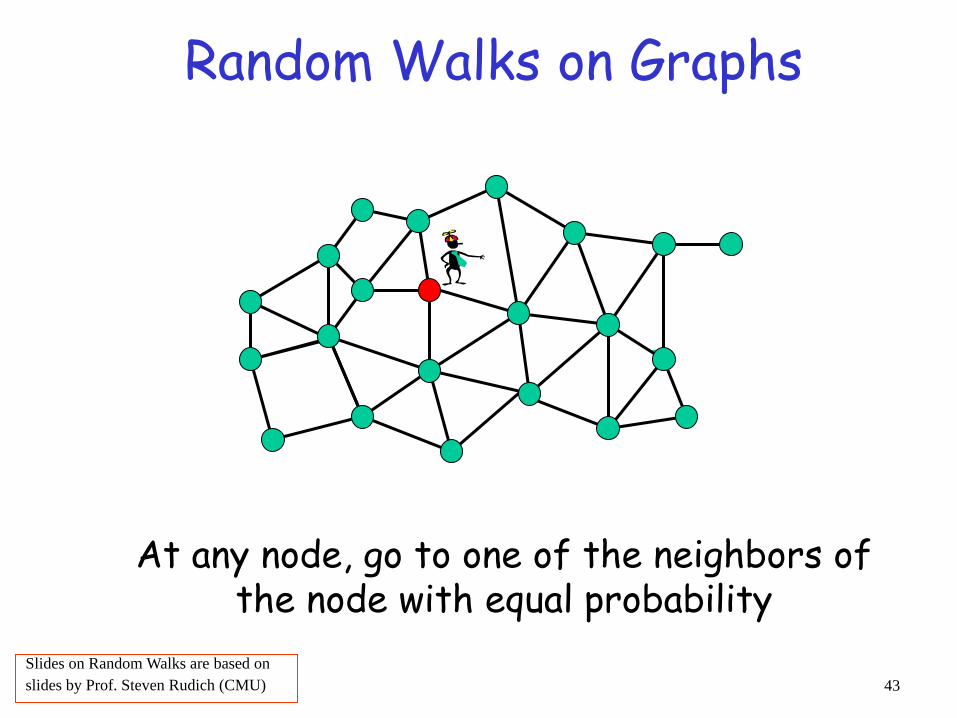
Random Walks on Graphs
At any node, go to one of the neighbors of the node with equal probability
Slides on Random Walks are based on
slides by Prof. Steven Rudich (CMU) 43
-
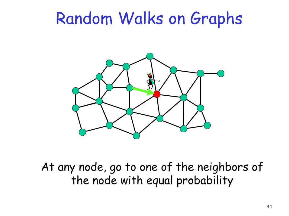
Random Walks on Graphs
At any node, go to one of the neighbors of the node with equal probability
44

-
Random Walks on Graphs
At any node, go to one of the neighbors of the node with equal probability
45
-
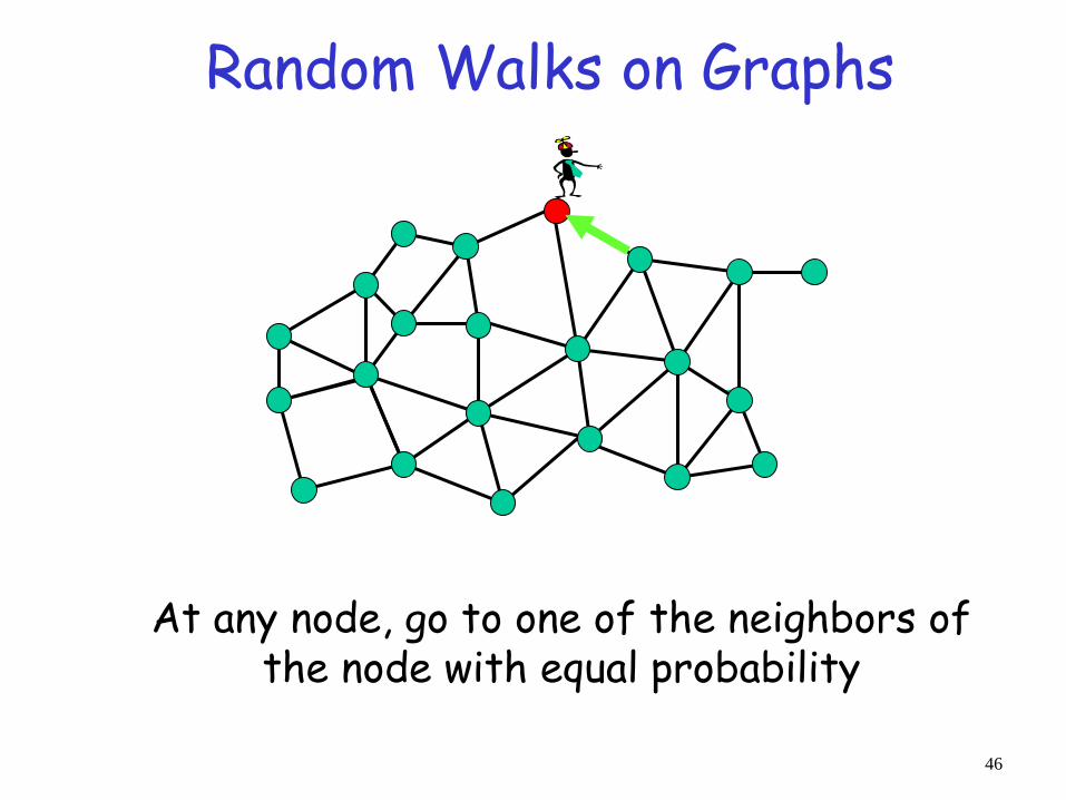
Random Walks on Graphs
At any node, go to one of the neighbors of the node with equal probability
46

-
Random Walks on Graphs
At any node, go to one of the neighbors of the node with equal probability
47

0 n
k
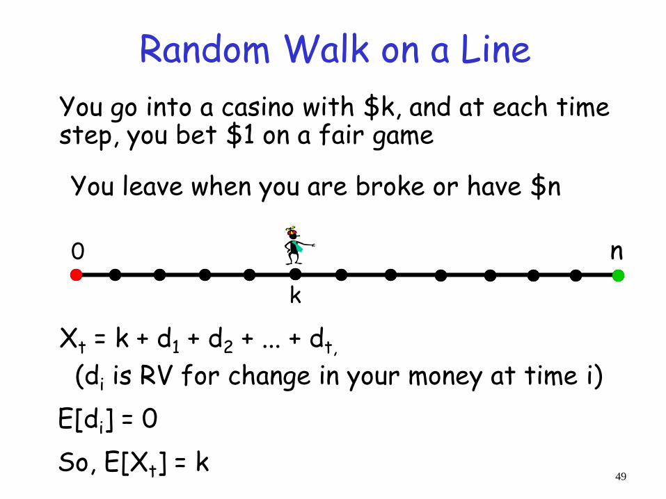
Random Walk on a Line
You go into a casino with $k, and at each time step, you bet $1 on a fair game
You leave when you are broke or have $n
Question 1: what is your expected amount of money at time t?
Let Xt be a R.V. for the amount of $ at time t
48
0 n
k
You go into a casino with $k, and at each time step, you bet $1 on a fair game
You leave when you are broke or have $n
Xt = k + d1 + d2 + ... + dt,
(di is RV for change in your money at time i)
So, E[Xt] = k
E[di] = 0
Random Walk on a Line
49
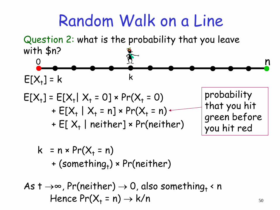
Question 2: what is the probability that you leave with $n?
E[Xt] = k
E[Xt] = E[Xt| Xt = 0] × Pr(Xt = 0)
+ E[Xt | Xt = n] × Pr(Xt = n)
+ E[ Xt | neither] × Pr(neither)
As t ∞, Pr(neither) 0, also somethingt < n Hence Pr(Xt = n) k/n
k = n × Pr(Xt = n)
+ (somethingt) × Pr(neither)
0
k
n
probability that you hit green before you hit red
Random Walk on a Line
50

Getting Back Home
-
Lost in a city, you want to get back to your hotel How should you do this?
Requires a good memory or a piece of chalk
Depth First Search!
51

Getting Back Home
-
How about walking randomly?
52
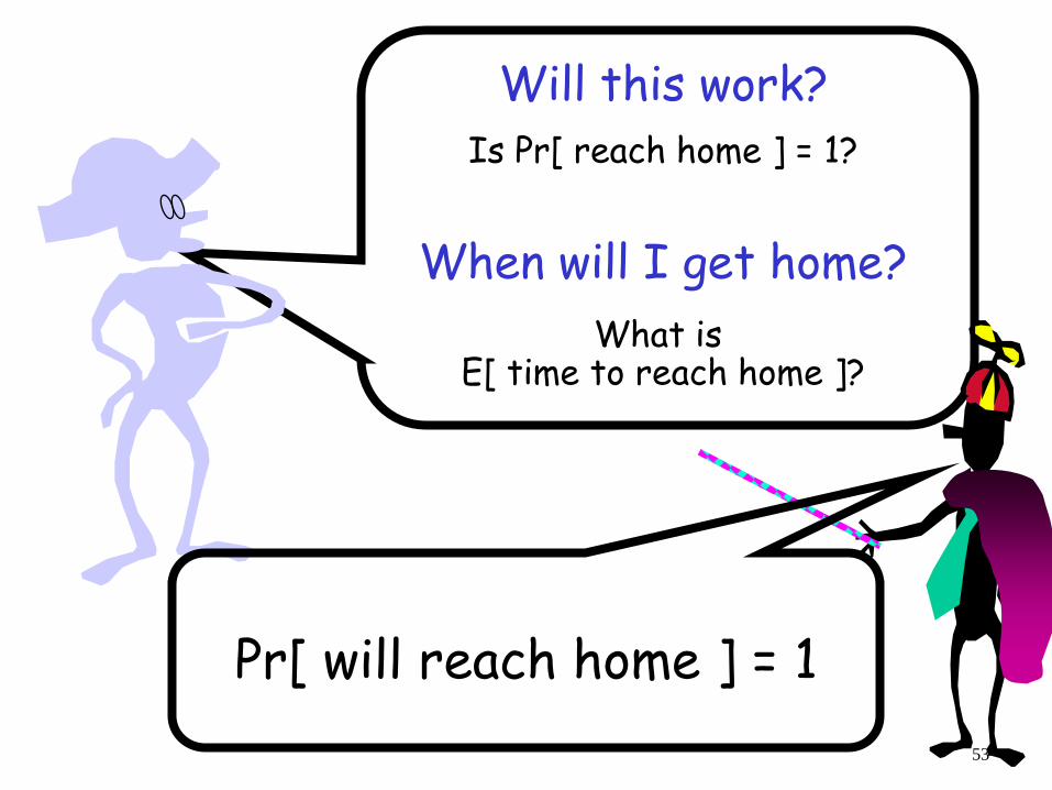
Will this work?
When will I get home?
Is Pr[ reach home ] = 1?
What is E[ time to reach home ]?
Pr[ will reach home ] = 1
53
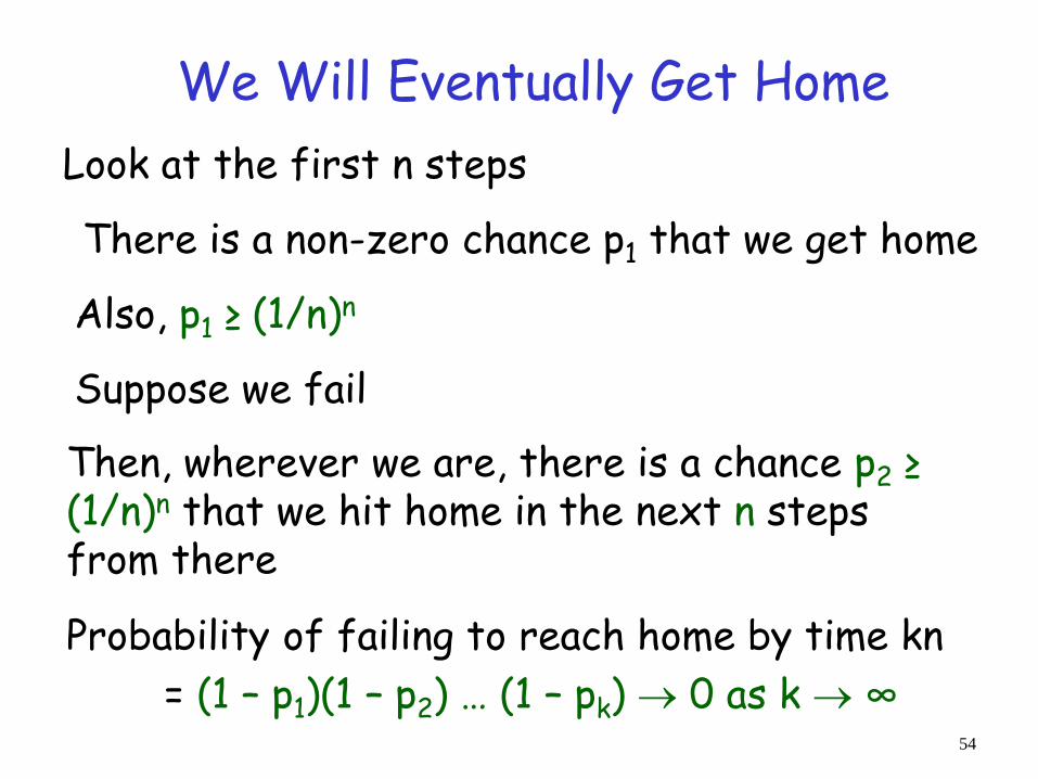
We Will Eventually Get Home
Look at the first n steps
There is a non-zero chance p1 that we get home
Also, p1 ≥ (1/n)n
Suppose we fail
Then, wherever we are, there is a chance p2 ≥ (1/n)n that we hit home in the next n steps from there
Probability of failing to reach home by time kn
= (1 – p1)(1 – p2) … (1 – pk) 0 as k ∞ 54

Furthermore:
If the graph has n nodes and m edges, then
E[ time to visit all nodes ] ≤ 2m × (n-1)
55

Cover Times
Cover time (from u) Cu = E [ time to visit all vertices | start at u ]
Cover time of the graph
(worst case expected time to see all vertices)
C(G) = maxu Cu
56
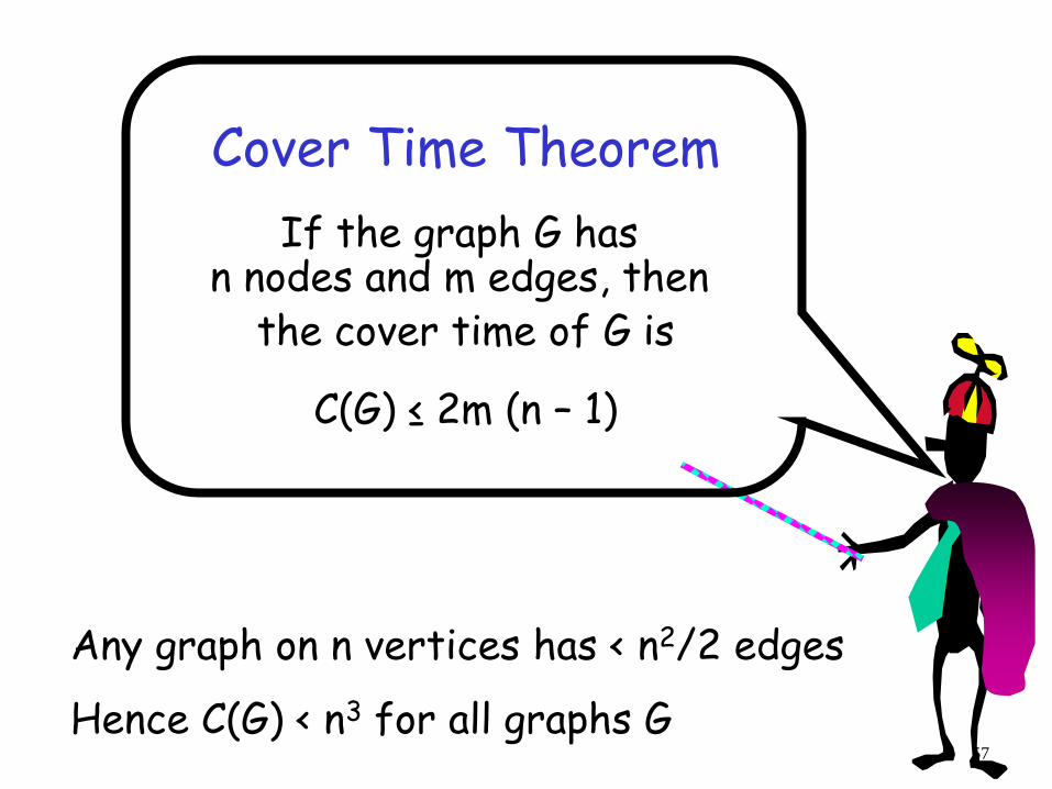
Cover Time Theorem
If the graph G has n nodes and m edges, then
the cover time of G is
C(G) ≤ 2m (n – 1)
Any graph on n vertices has < n2/2 edges
Hence C(G) < n3 for all graphs G 57

Actually, we get home pretty fast…
Chance that we don’t hit home by
(2k)2m(n-1) steps is (½)k
Why?
58

Random Walks are useful
• Efficient sampling from complicated distributions
• Ranking (search results, web pages, friend suggestions, spam detection)
• Clustering
• Design and analysis of random data structures and algorithms
• Applications in physics, economics, biology…
• Much more…..
59

Cut Problems
• Definition: A Cut S in the graph G(V; E) is a vertex partitioning into two sets: S and S’ such that S S’= V .
• The edges in the cut (S;S’) are those connecting a vertex in S and a vertex in S’.
S S’
The cut defined by S 60
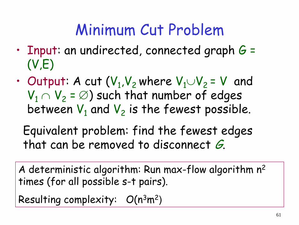
Minimum Cut Problem • Input: an undirected, connected graph G =
(V,E)
• Output: A cut (V1,V2 where V1V2 = V and V1 V2 = ) such that number of edges between V1 and V2 is the fewest possible.
Equivalent problem: find the fewest edges that can be removed to disconnect G.
A deterministic algorithm: Run max-flow algorithm n2 times (for all possible s-t pairs).
Resulting complexity: O(n3m2( 61
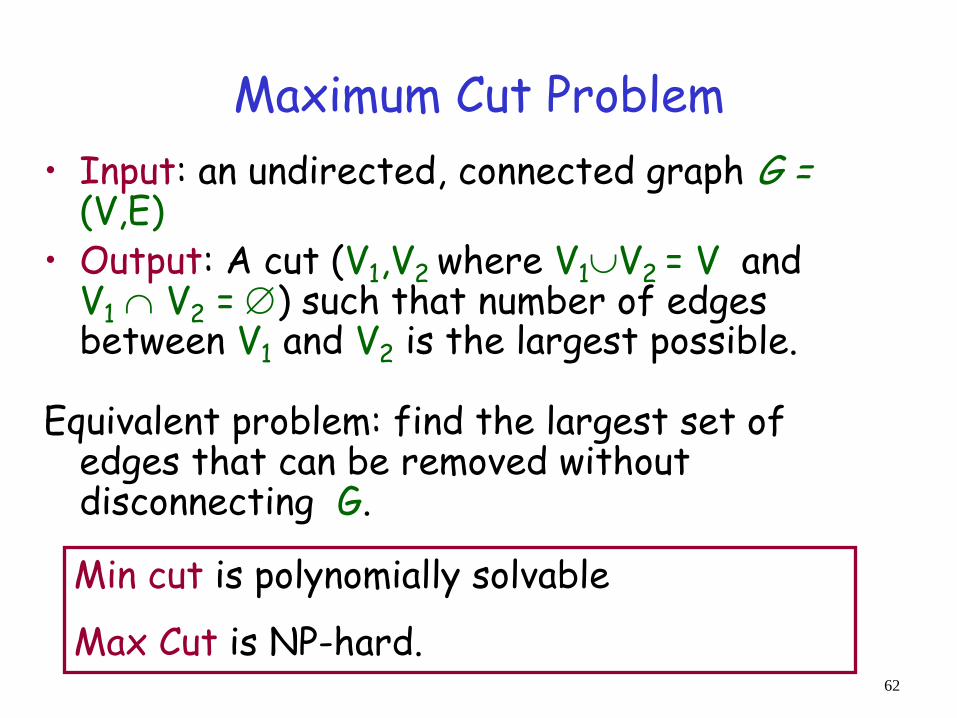
Maximum Cut Problem
• Input: an undirected, connected graph G = (V,E)
• Output: A cut (V1,V2 where V1V2 = V and V1 V2 = ) such that number of edges between V1 and V2 is the largest possible.
Equivalent problem: find the largest set of
edges that can be removed without disconnecting G.
Min cut is polynomially solvable
Max Cut is NP-hard. 62
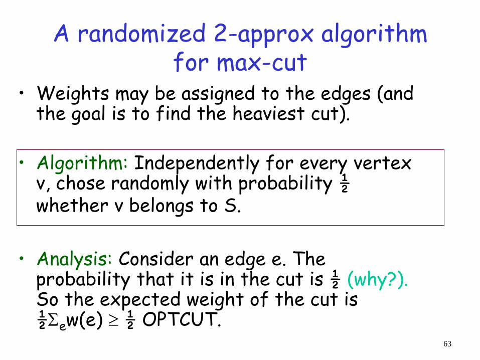
A randomized 2-approx algorithm for max-cut
• Weights may be assigned to the edges (and the goal is to find the heaviest cut).
• Algorithm: Independently for every vertex v, chose randomly with probability ½ whether v belongs to S.
• Analysis: Consider an edge e. The probability that it is in the cut is ½ (why?). So the expected weight of the cut is ½ew(e) ½ OPTCUT.
63

A randomized 2-approx algorithm for max-cut
Remarks:
• We can run the algorithm a few times to improve its performance – getting closer to guaranteeing 2-approx.
• Corollary: There exists a cut having weight at least ½ew(e).
64
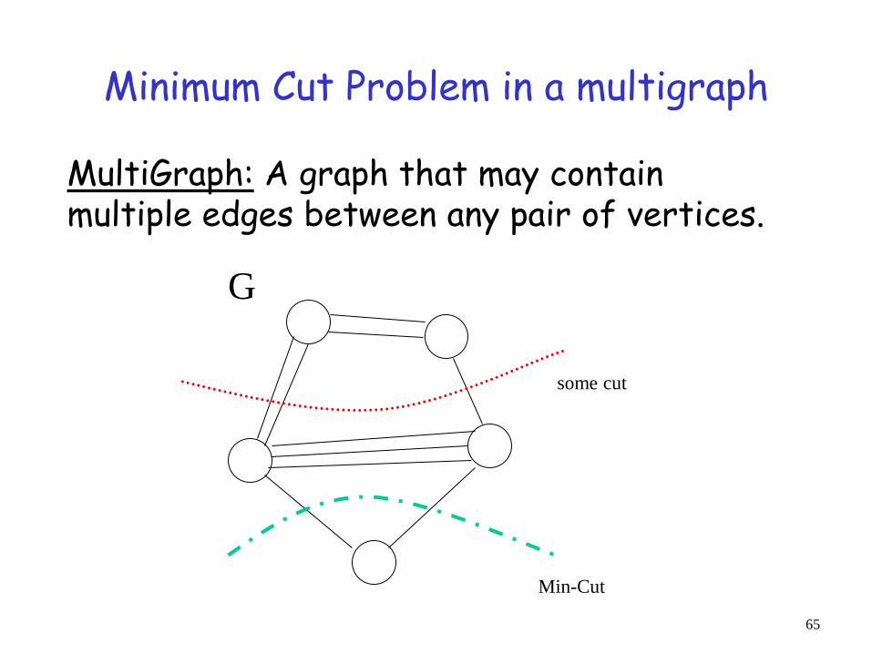
Minimum Cut Problem in a multigraph
MultiGraph: A graph that may contain multiple edges between any pair of vertices.
Min-Cut
some cut
G
65

Minimum Cut
A
B
C
D
Size of the min cut is not larger than the smallest node degree in graph
E
G
F
H
A
B
C
D
But can be much smaller… 66
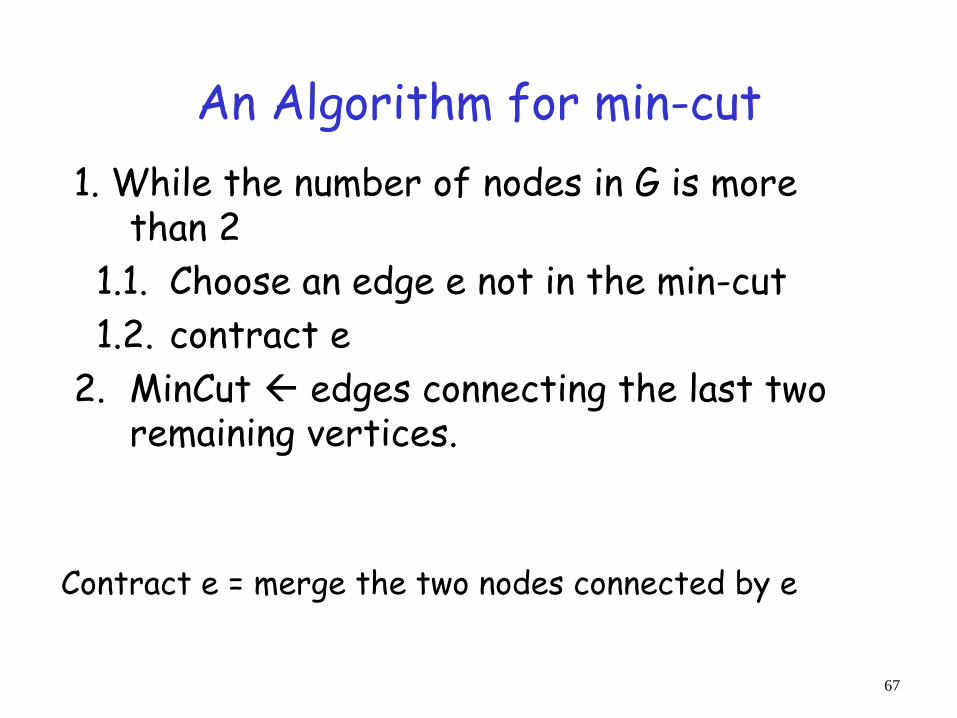
An Algorithm for min-cut
1. While the number of nodes in G is more than 2
1.1. Choose an edge e not in the min-cut
1.2. contract e
2. MinCut edges connecting the last two remaining vertices.
67
Contract e = merge the two nodes connected by e

An Algorithm for min-cut
1. While the number of nodes in G is more than 2
1.1. Choose an edge e not in the min-cut
1.2. contract e
2. MinCut edges connecting the last two remaining vertices.
68
randomly
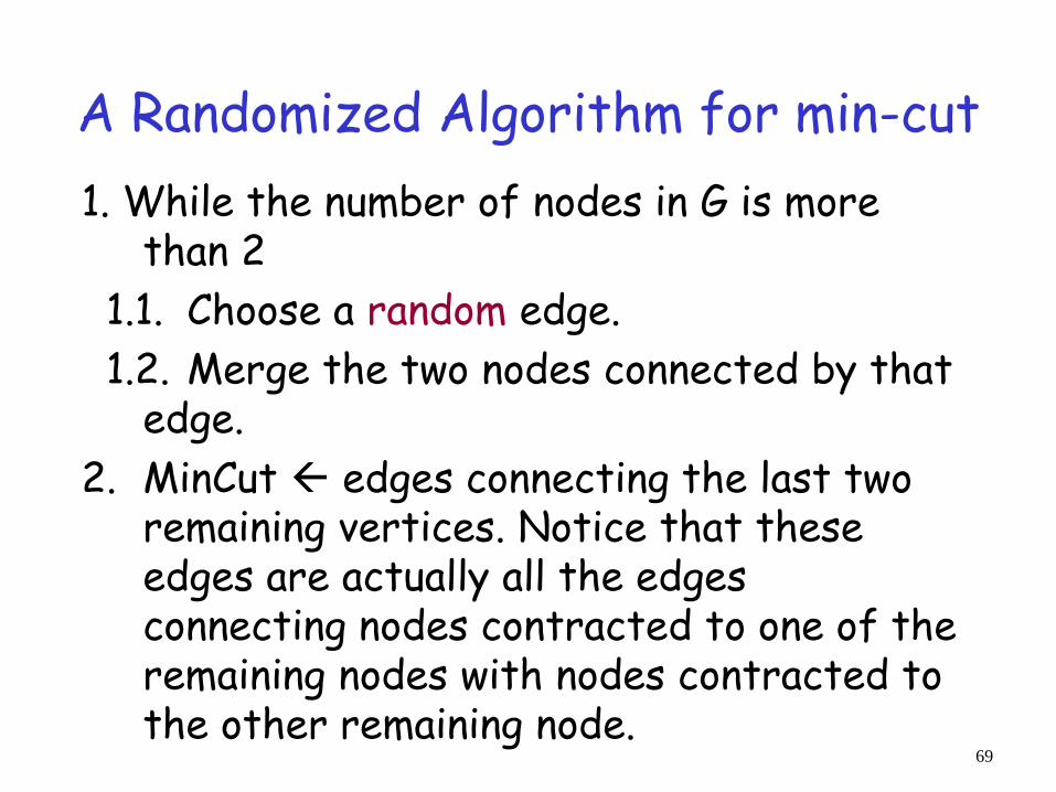
A Randomized Algorithm for min-cut
1. While the number of nodes in G is more than 2
1.1. Choose a random edge.
1.2. Merge the two nodes connected by that edge.
2. MinCut edges connecting the last two remaining vertices. Notice that these edges are actually all the edges connecting nodes contracted to one of the remaining nodes with nodes contracted to the other remaining node.
69

Running example
1 2
3 4
5
1 2
,43
5
Iteration 1: Iteration 2:
70

Running example (cont’)
1,2
,43
5
,431,2,
5
G 1
2
3 4
5
stop: the cut separates the vertices sets 5 and 1,2,3,4
Iteration 3: Iteration 4: Output:
71

Min-Cut algorithm analysis
Will this algorithm return the Min-Cut?
Let C be a particular Min-Cut. Let k be size of C.
The algorithm will return C if it never contracts any edge of C.
We need to estimate the probability that in each iteration it chooses an edge not from C.
72

Min-Cut algorithm analysis (cont’)
• The probability of picking at each iteration an edge from C is k/|E|, where |E| is the number of edges still in G.
• There is no vertex with degree less than k (we already mentioned that k ≤ minimal degree)
• So |E| = (sum of degrees)/2 ≥ kn/2
• Therefore, the probability of choosing an edge from C in iteration i is at most
1in
2
2k1)i(n
k
Note: In iteration i there are n-i+1 nodes.
73

Min-Cut algorithm analysis (cont’)
• Define ei to be the event of not choosing an edge
from C in iteration i.
•The probability of not choosing an edge from C in
iteration i (assuming not chosen earlier) is at least
• The probability of not choosing an edge from C at
all is:
1
21
in
n
21Pr 1 e
Pr 휀𝑖
𝑛−2
𝑖=1
≥ 1−2
𝑛 − 𝑖 + 1=
𝑛−2
𝑖=1
(𝑛 − 𝑗 + 1)𝑛𝑗=3
(𝑛 − 𝑖 + 1)𝑛−2𝑖=1
=2
𝑛(𝑛 − 1)
74
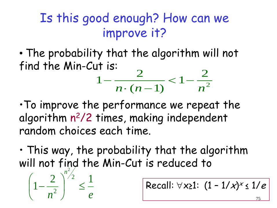
Is this good enough? How can we improve it?
• The probability that the algorithm will not find the Min-Cut is:
•To improve the performance we repeat the algorithm n2/2 times, making independent random choices each time.
• This way, the probability that the algorithm will not find the Min-Cut is reduced to
en
n
121
2
2
2
2
21
)1(
21
nnn
Recall: x≥1: (1 – 1/x)x ≤ 1/e
75
Primality Testing • Public-Key Cryptography needs large prime
numbers
• How can you tell if p is prime? – Try dividing p by all smaller integers
• Exponential in |p| (number of bits to represent p)
– Improvement: try only smaller primes • Still exponential
• Until 2002 no deterministic Poly-time test was known! – Agrawal-Kayal-Saxena showed (inefficient) test
– Much more efficient randomized tests exist. 76

Fermat’s (little) Theorem
• If p is a prime then for all a, 𝑎𝑝−1 ≡ 1 mod 𝑝
• Randomized test for a number n: – Choose a random a between 1 and n-1
– Check if 𝑎𝑛−1 ≡ 1 mod 𝑛
– If not, n is definitely not prime
• What is the probability of error? 77

Fermat Primality Test • If 𝑎𝑛−1 ≢ 1 mod 𝑛 we call a a “Fermat
Witness” for the compositeness of n
• For composite n, if 𝑏𝑛−1 ≡ 1 mod 𝑛 (b≠1) we call b a “Fermat Liar”
• Claim: if a is a Fermat witness for n, then at least half the a’s are Fermat witnesses
• Proof: Let b1,…,bk be Fermat liars. Then (𝑎 ⋅ 𝑏𝑖)
𝑛−1≡ 𝑎𝑛−1𝑏𝑖𝑛−1 ≡ 𝑎𝑛−1 ⋅ 1 ≢ 1 mod 𝑛
– So ab1,…,abk are all Fermat witnesses!
78
Fermat Primality Test • So, error probability at most ½?
• No: we assumed there exists a Fermat witness.
– There is an infinite sequence of composites that have no Fermat witnesses at all: the Carmichael Numbers
• Fermat primality test will always fail for Carmichael numbers.
– They are rarer than primes, but still a problem.
• Slightly more complex test (Rabin-Miller) always works
79