Lecture 14, p 1

Lecture 14: Superposition & Time-Dependent Quantum States

x

|y(x,t0)|2

U= U=

0 x L

|y(x,t=0)|2 U= U=

0 x L

Lecture 14, p 2

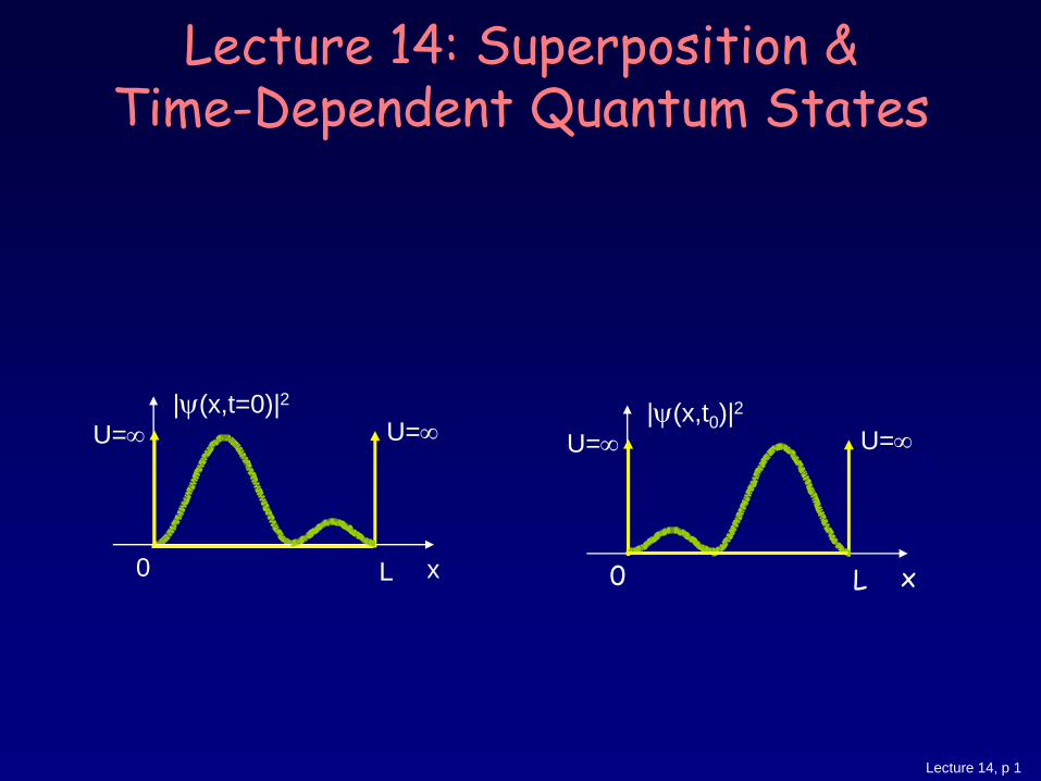
Last Week Time-independent Schrodinger’s Equation (SEQ):

It describes a particle that has a definite energy, E.

The solutions, y(x), are time independent (stationary states).

We considered three potentials, U(x):

Infinite square well

Boundary conditions only certain allowed energies (and

corresponding “energy eigenstates”)

Finite-depth square well

Particle can “leak” into forbidden region.

Comparison with infinite-depth well.

Harmonic oscillator

Energy levels are equally spaced.

A good approximation in many problems.

)()()()(

2 2

22

xExxUdx

xd

myy

y

Lecture 14, p 3

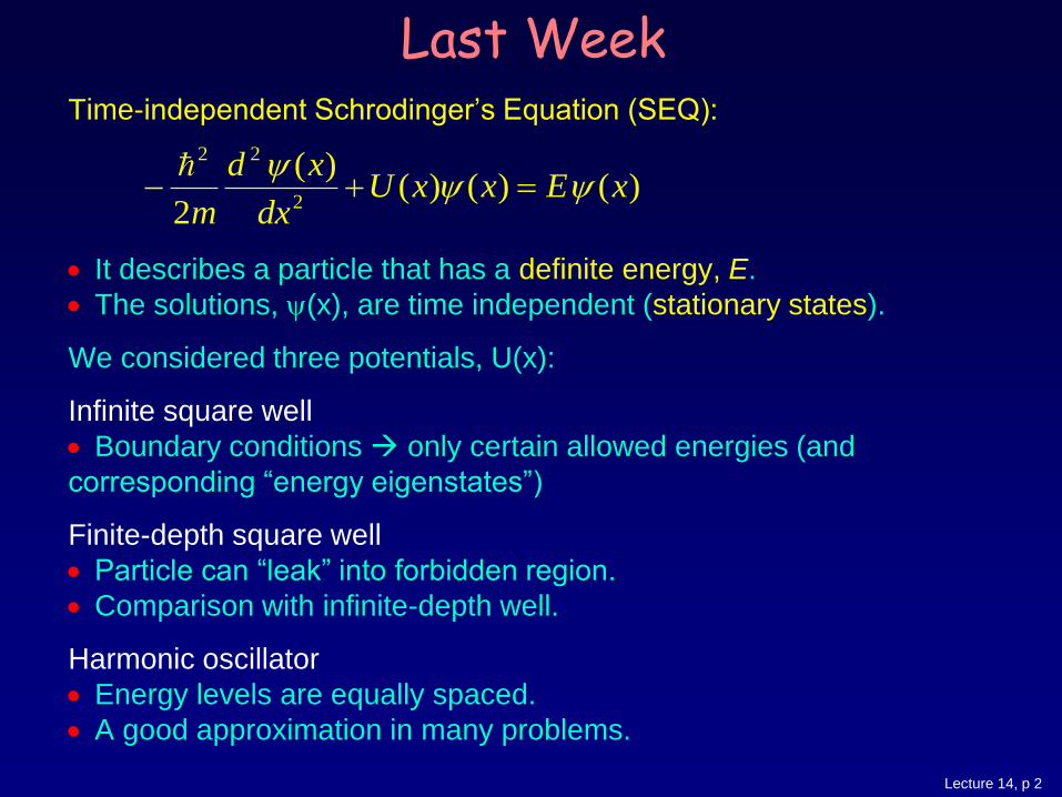
Today

Time dependent SEQ: Superposition of states and particle motion

Measurement in quantum physics

Time-energy uncertainty principle

Lecture 14, p 4

Lecture 14, p 5

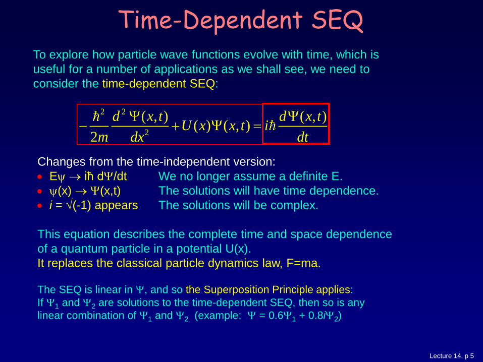
Time-Dependent SEQ To explore how particle wave functions evolve with time, which is

useful for a number of applications as we shall see, we need to

consider the time-dependent SEQ:

Changes from the time-independent version:

Ey iħ dY/dt We no longer assume a definite E.

y(x) Y(x,t) The solutions will have time dependence.

i = (-1) appears The solutions will be complex.

This equation describes the complete time and space dependence

of a quantum particle in a potential U(x).

It replaces the classical particle dynamics law, F=ma.

The SEQ is linear in Y, and so the Superposition Principle applies:

If Y1 and Y2 are solutions to the time-dependent SEQ, then so is any

linear combination of Y1 and Y2 (example: Y = 0.6Y1 + 0.8iY2)

2 2

2

( , ) ( , )( ) ( , )

2

d x t d x tU x x t i

m dx dt

Y Y Y

Lecture 14, p 6

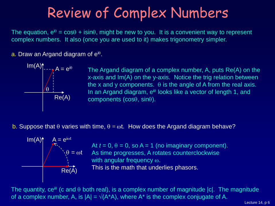
Review of Complex Numbers The equation, eiq = cosq + isinq, might be new to you. It is a convenient way to represent

complex numbers. It also (once you are used to it) makes trigonometry simpler.

a. Draw an Argand diagram of eiq.

The Argand diagram of a complex number, A, puts Re(A) on the

x-axis and Im(A) on the y-axis. Notice the trig relation between

the x and y components. q is the angle of A from the real axis.

In an Argand diagram, eiq looks like a vector of length 1, and

components (cosq, sinq). Re(A)

Im(A)

q

A = eiq

The quantity, ceiq (c and q both real), is a complex number of magnitude |c|. The magnitude

of a complex number, A, is |A| = (A*A), where A* is the complex conjugate of A.

Re(A)

Im(A)

q = wt

A = eiwt

b. Suppose that q varies with time, q = wt. How does the Argand diagram behave?

At t = 0, q = 0, so A = 1 (no imaginary component).

As time progresses, A rotates counterclockwise

with angular frequency w.

This is the math that underlies phasors.

Lecture 14, p 7

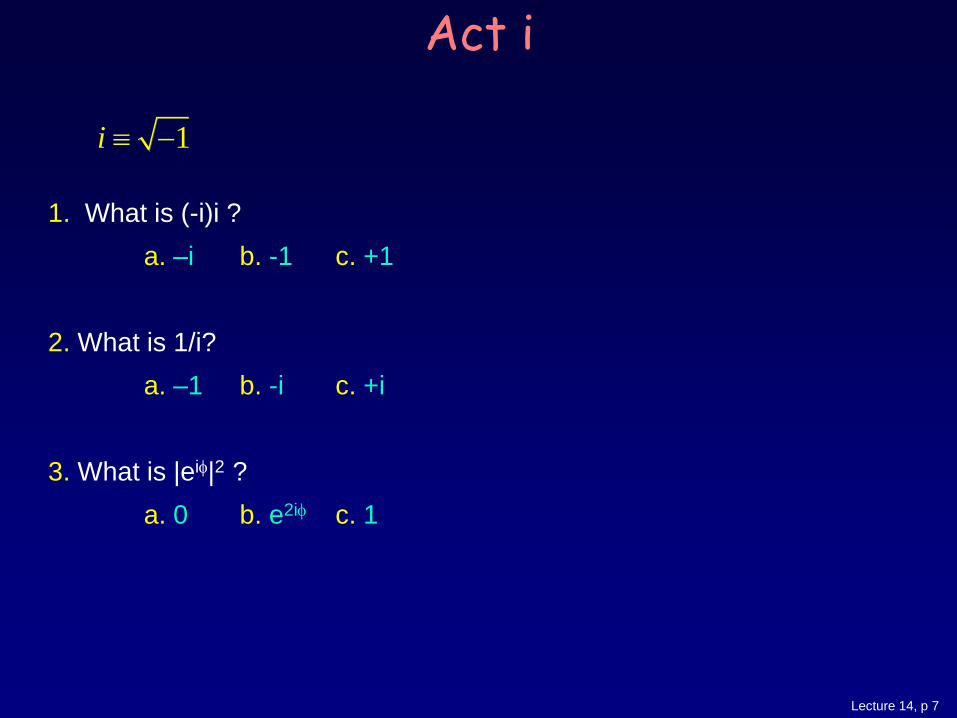
Act i

1. What is (-i)i ?

a. –i b. -1 c. +1

2. What is 1/i?

a. –1 b. -i c. +i

3. What is |ei|2 ?

a. 0 b. e2i c. 1

1i

Lecture 14, p 8

Lecture 14, p 9

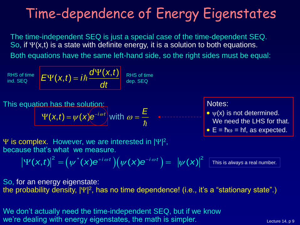
Time-dependence of Energy Eigenstates

The time-independent SEQ is just a special case of the time-dependent SEQ. So, if Y(x,t) is a state with definite energy, it is a solution to both equations.

Both equations have the same left-hand side, so the right sides must be equal:

This equation has the solution:

Y is complex. However, we are interested in |Y|2, because that’s what we measure.

So, for an energy eigenstate: the probability density, |Y|2, has no time dependence! (i.e., it’s a “stationary state”.)

We don’t actually need the time-independent SEQ, but if we know we’re dealing with energy eigenstates, the math is simpler.

( , ) h it( w) i t Ex t x e wy wY

2 2*( , ) ( ) ( ) ( )i t i tx t x e x e xw wy y y Y

( , )( , )

d x tE x t i

dt

YY

RHS of time

ind. SEQ RHS of time

dep. SEQ

Notes:

y(x) is not determined.

We need the LHS for that.

E = ħw = hf, as expected.

This is always a real number.

Lecture 14, p 10

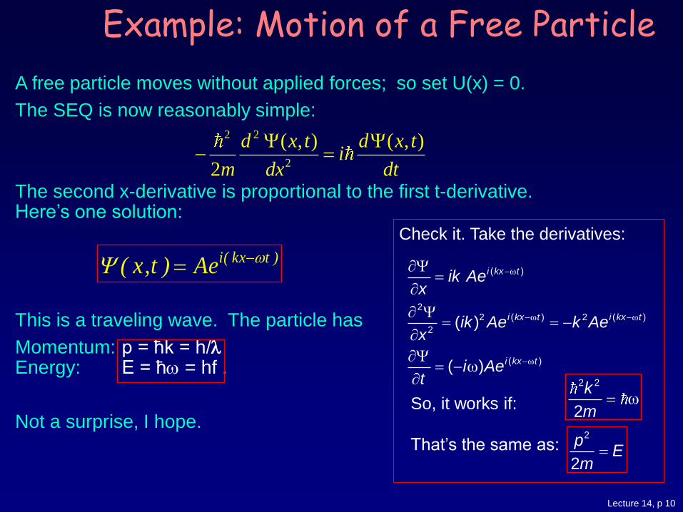
Example: Motion of a Free Particle

A free particle moves without applied forces; so set U(x) = 0.

The SEQ is now reasonably simple:

The second x-derivative is proportional to the first t-derivative. Here’s one solution:

This is a traveling wave. The particle has

Momentum: p = ħk = h/l Energy: E = ħw = hf .

Not a surprise, I hope.

2 2

2

( , ) ( , )

2

d x t d x ti

m dx dt

Y Y

)tkx(iAe)t,x( wY ( )

22 ( ) 2 ( )

2

( )

( )

( )

i kx t

i kx t i kx t

i kx t

ik Aex

ik Ae k Aex

i Aet

w

w w

w

Y

Y

Y w

Check it. Take the derivatives:

2 2

2

k

m wSo, it works if:

That’s the same as: 2

2

pE

m

Lecture 14, p 11

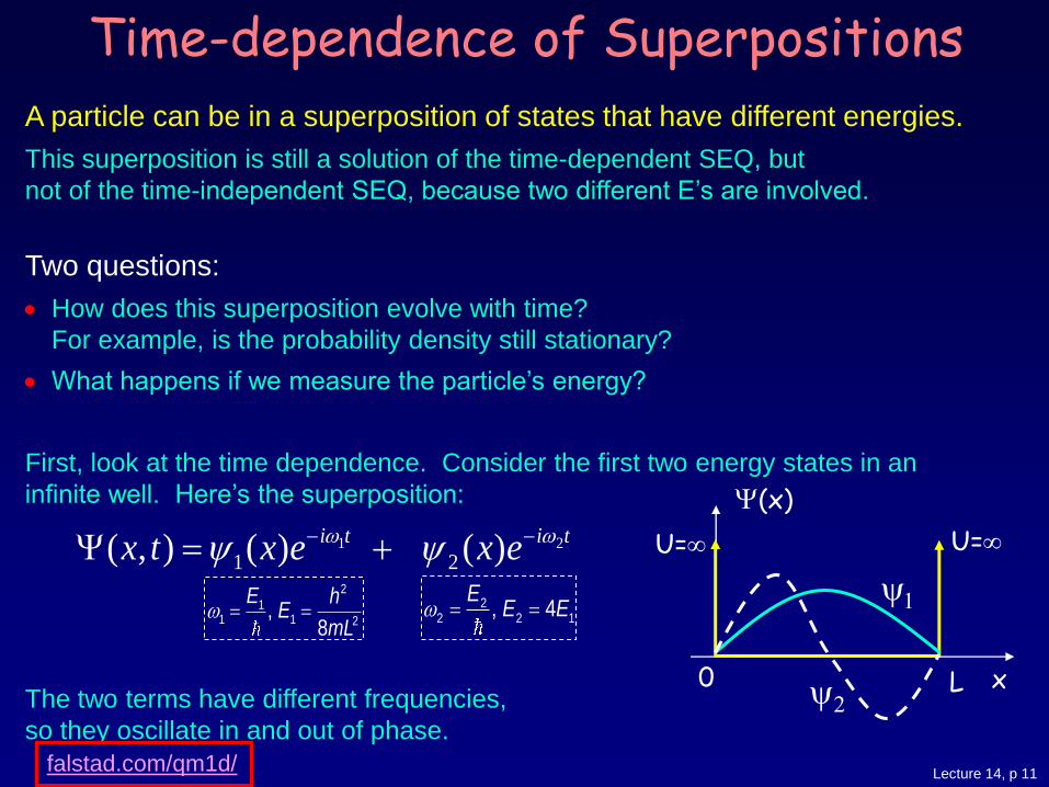
Time-dependence of Superpositions A particle can be in a superposition of states that have different energies.

This superposition is still a solution of the time-dependent SEQ, but

not of the time-independent SEQ, because two different E’s are involved.

Two questions:

How does this superposition evolve with time?

For example, is the probability density still stationary?

What happens if we measure the particle’s energy?

First, look at the time dependence. Consider the first two energy states in an

infinite well. Here’s the superposition:

The two terms have different frequencies,

so they oscillate in and out of phase.

U= U=

Y(x)

0 L x

y1

y2

1 2

1 2( , ) ( ) ( )w wy y Y i t i tx t x e x e

22 2 1, 4

EE Ew

2

11 1 2

, 8

E hE

mLw

falstad.com/qm1d/

Lecture 14, p 12

Lecture 14, p 13

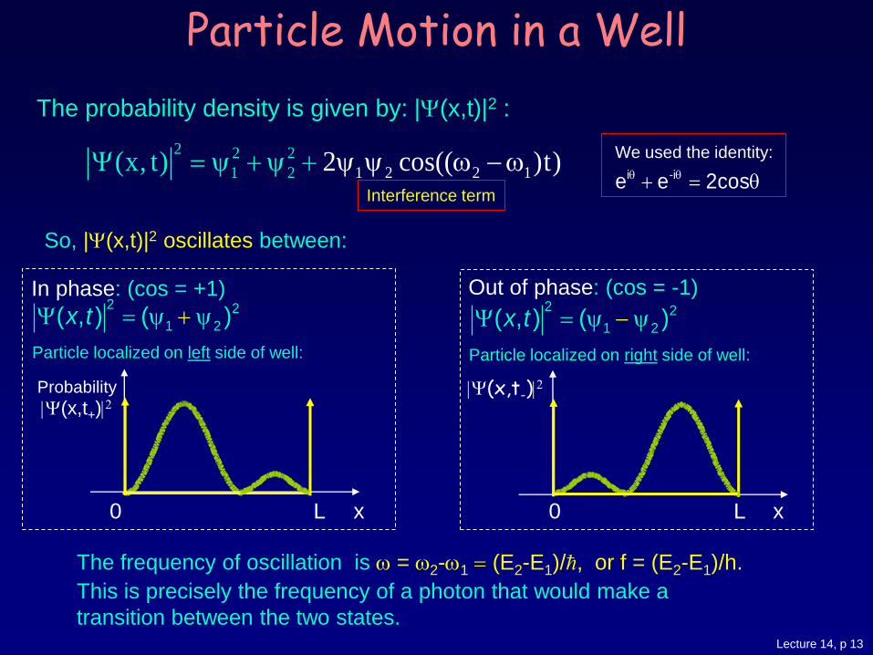
Particle Motion in a Well

The frequency of oscillation is w = w2-w1 (E2-E1)/, or f = (E2-E1)/h.

This is precisely the frequency of a photon that would make a

transition between the two states.

So, |Y(x,t)|2 oscillates between:

i -ie e 2cosq q q

We used the identity:

The probability density is given by: |Y(x,t)|2 :

1 2 21 2 1

2 2 2 2 cos(( )t)(x, t) y y w wY y y Interference term

2 2

1 2( , ) ( )x tY y y

Particle localized on left side of well:

|Y(x,t+)|2

0 x L

Probability

In phase: (cos = +1)

Particle localized on right side of well:

|Y(x,t-)|2

0 x L

Out of phase: (cos = -1) 2 2

1 2( , ) ( )x tY y y

Lecture 14, p 14

Interference Beats

The motion of the probability density comes from the changing interference between terms in Y that have different energy.

The beat frequency between two terms is the frequency difference, f2 - f1.

So energy differences are important: E1 - E2 = hf1 - hf2, etc.

Just like in Newtonian physics: absolute energies aren’t important (you can pick where to call U=0 for convenience), only energy differences.

Lecture 14, p 15

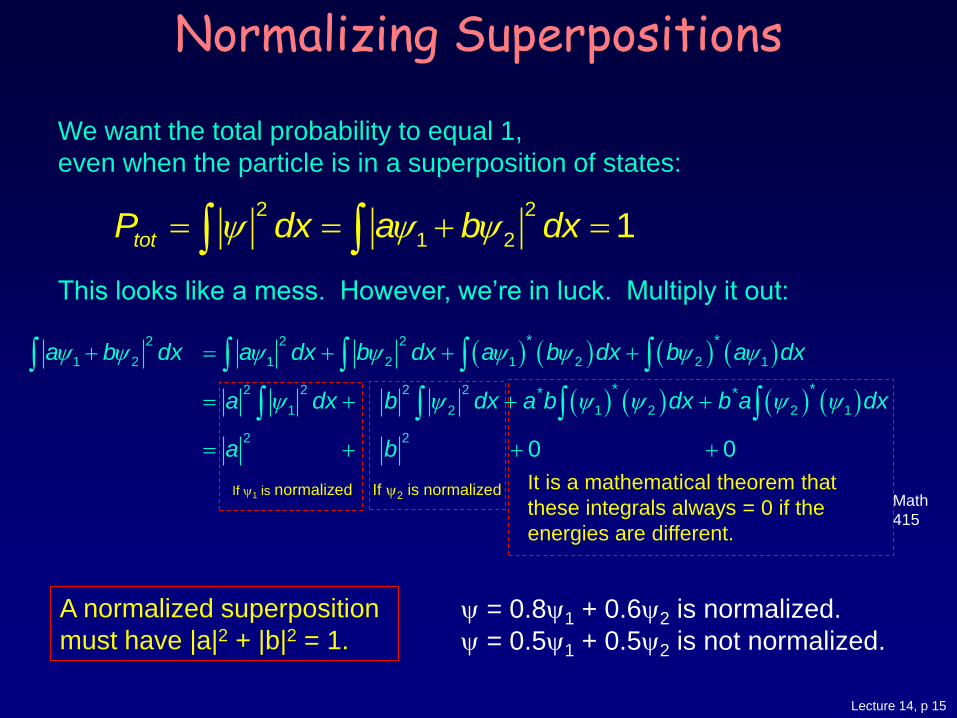
Normalizing Superpositions

We want the total probability to equal 1,

even when the particle is in a superposition of states:

This looks like a mess. However, we’re in luck. Multiply it out:

2 2

1 2 1totP dx a b dxy y y

y y y y y y y y

y y y y y y

2 2 2

1 2 1 2 1 2 2 1

2 2 2 2

1 2 1 2 2 1

2 2

* *

* ** *

0 0

a b dx a dx b dx a b dx b a dx

a dx b dx a b dx b a dx

a b

If y1 is normalized If y2 is normalized It is a mathematical theorem that

these integrals always = 0 if the

energies are different.

A normalized superposition

must have |a|2 + |b|2 = 1.

y = 0.8y1 + 0.6y2 is normalized.

y = 0.5y1 + 0.5y2 is not normalized.

Math

415

Lecture 14, p 16

Lecture 14, p 17

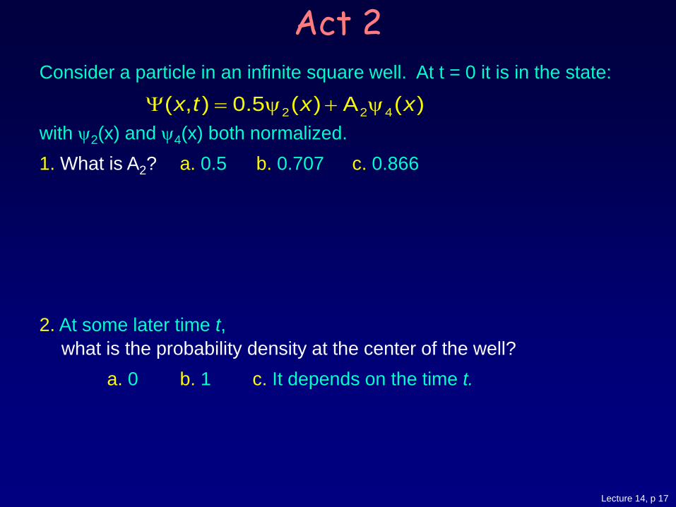
Consider a particle in an infinite square well. At t = 0 it is in the state:

with y2(x) and y4(x) both normalized.

1. What is A2? a. 0.5 b. 0.707 c. 0.866

2. At some later time t,

what is the probability density at the center of the well?

a. 0 b. 1 c. It depends on the time t.

Act 2

2 2 4( , ) 0.5 ( ) A ( )x t x xY y y

Lecture 14, p 18

Measurements of Energy

We are now ready to deal with the second question from earlier in the lecture:

What happens when we measure the energy of a particle whose wave function is a superposition of more than one energy state?

If the wave function is in an energy eigenstate (E1, say), then we know with certainty that we will obtain E1 (unless the apparatus is broken).

If the wave function is a superposition (y = ay1+by2) of energies E1 and E2, then we aren’t certain what the result will be. However: We know with certainty that we will only obtain E1 or E2 !!

To be specific, we will never obtain (E1+E2)/2, or any other value.

What about a and b? |a|2 and |b|2 are the probabilities of obtaining E1 and E2, respectively. That’s why we normalize the wave function to make |a|2 + |b|2 =1.

We can’t prove

this statement. It

is one of the

fundamental

postulates of

quantum theory.

Treat it as an

empirical fact.

Lecture 14, p 19

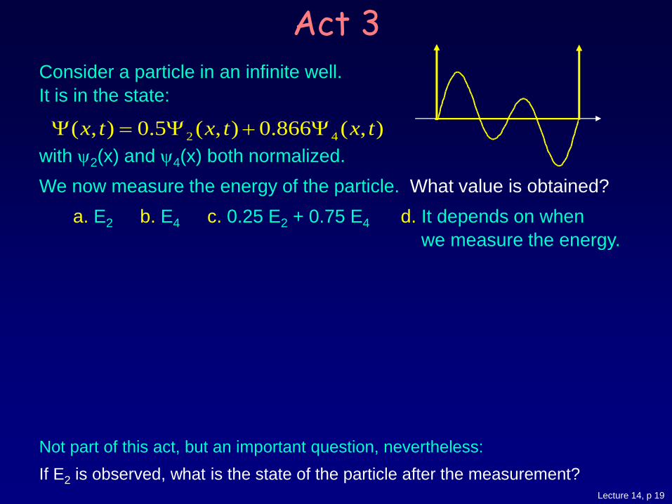
Consider a particle in an infinite well.

It is in the state:

with y2(x) and y4(x) both normalized.

We now measure the energy of the particle. What value is obtained?

a. E2 b. E4 c. 0.25 E2 + 0.75 E4 d. It depends on when

we measure the energy.

Not part of this act, but an important question, nevertheless:

If E2 is observed, what is the state of the particle after the measurement?

Act 3

2 4( , ) 0.5 ( , ) 0.866 ( , )Y Y Yx t x t x t

Lecture 14, p 20

Lecture 14, p 21

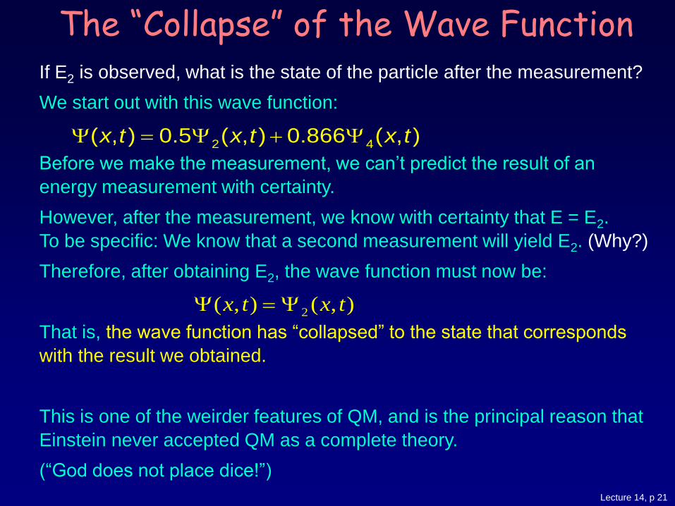
If E2 is observed, what is the state of the particle after the measurement?

We start out with this wave function:

Before we make the measurement, we can’t predict the result of an

energy measurement with certainty.

However, after the measurement, we know with certainty that E = E2.

To be specific: We know that a second measurement will yield E2. (Why?)

Therefore, after obtaining E2, the wave function must now be:

That is, the wave function has “collapsed” to the state that corresponds

with the result we obtained.

This is one of the weirder features of QM, and is the principal reason that

Einstein never accepted QM as a complete theory.

(“God does not place dice!”)

The “Collapse” of the Wave Function

2 4( , ) 0.5 ( , ) 0.866 ( , )x t x t x tY Y Y

2( , ) ( , )Y Yx t x t

Lecture 14, p 22

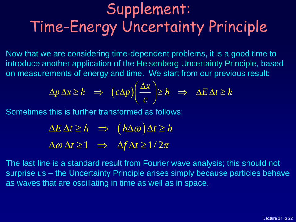
Supplement: Time-Energy Uncertainty Principle

Now that we are considering time-dependent problems, it is a good time to

introduce another application of the Heisenberg Uncertainty Principle, based

on measurements of energy and time. We start from our previous result:

Sometimes this is further transformed as follows:

The last line is a standard result from Fourier wave analysis; this should not

surprise us – the Uncertainty Principle arises simply because particles behave

as waves that are oscillating in time as well as in space.

x

p x c p E tc

1 1/ 2

E t t

t f t

w

w

Lecture 14, p 23

14

15

1 2 1

1/ 2

1/(2 0.4 10 Hz)

s 44 fs10

t f t

t f

w

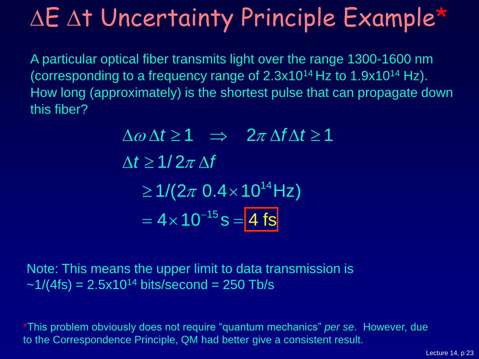
A particular optical fiber transmits light over the range 1300-1600 nm

(corresponding to a frequency range of 2.3x1014 Hz to 1.9x1014 Hz).

How long (approximately) is the shortest pulse that can propagate down

this fiber?

E t Uncertainty Principle Example*

Note: This means the upper limit to data transmission is

~1/(4fs) = 2.5x1014 bits/second = 250 Tb/s

*This problem obviously does not require “quantum mechanics” per se. However, due

to the Correspondence Principle, QM had better give a consistent result.

Lecture 14, p 24

Lecture 14, p 25

Next Week

3-Dimensional Potential Well

Schrödinger’s Equation for the Hydrogen Atom

Lecture 14, p 26

Supplement: Quantum Information References

Quantum computing

Employs superpositions of quantum states - astoundingly good for certain parallel computation, may use entangled states for error checking

www.newscientist.com/nsplus/insight/quantum/48.html

http://www.cs.caltech.edu/~westside/quantum-intro.html

Quantum cryptography

Employs single photons or entangled pairs of photons to generate a secret key. Can determine if there has been eavesdropping in information transfer

cam.qubit.org/articles/crypto/quantum.php

library.lanl.gov/cgi-bin/getfile?00783355.pdf

Quantum teleportation

Employs an entangled state to produce an exact replica of a third quantum state at a different point in space

www.research.ibm.com/quantuminfo/teleportation

www.quantum.univie.ac.at/research/photonentangle/teleport/index.html

Scientific American, April 2000

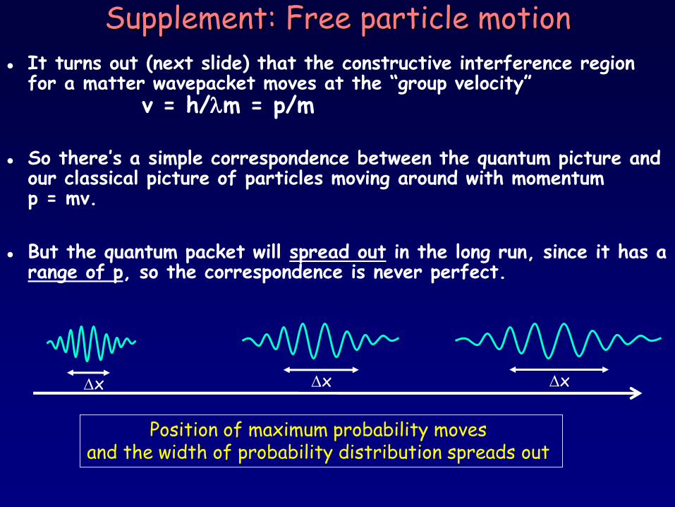
Supplement: Free particle motion

It turns out (next slide) that the constructive interference region for a matter wavepacket moves at the “group velocity” v = h/lm = p/m

So there’s a simple correspondence between the quantum picture and our classical picture of particles moving around with momentum p = mv.

But the quantum packet will spread out in the long run, since it has a range of p, so the correspondence is never perfect.

Position of maximum probability moves and the width of probability distribution spreads out

x x x

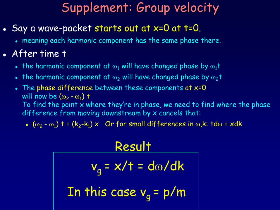
Supplement: Group velocity

Say a wave-packet starts out at x=0 at t=0. meaning each harmonic component has the same phase there.

After time t the harmonic component at w1 will have changed phase by w1t

the harmonic component at w2 will have changed phase by w2t

The phase difference between these components at x=0 will now be (w2 - w1) t To find the point x where they’re in phase, we need to find where the phase difference from moving downstream by x cancels that:

(w2 - w1) t = (k2-k1) x Or for small differences in w,k: tdw = xdk

Result

vg = x/t = dw/dk

In this case vg = p/m