THE TEMPERATURE DEPENDENT NON-LINEAR RESPONSE … · THE TEMPERATURE DEPENDENT NON-LINEAR RESPONSE...

THE TEMPERATURE DEPENDENT NON-LINEAR RESPONSE

OF A WOOD PLASTIC COMPOSITE

By

DOUGLAS J. POOLER

A thesis submitted in partial fulfillment of the requirements for the degree of

MASTER OF SCIENCE IN MECHANICAL ENGINEERING

WASHINGTON STATE UNIVERSITY Department of Mechanical and Materials Engineering

August 2001

ii

To the Faculty of Washington State University: The Members of the Committee appointed to examine the thesis of

Douglas J. Pooler find it satisfactory and recommend that it be accepted.

______________________________ Chair ______________________________ ______________________________

iii

ACKNOWLEDGMENT

The author would like to gratefully acknowledge the following for their support

and contribution to this work:

• Dr. Lloyd Smith: for serving on my committee, for his insight and expertise in the

matters of polymer and composite viscoelasticity, his patience, and his friendship.

• Dr. Michael Wolcott: for serving on my committee, for the time he spent discussing

the project, and the guidance he gave me, and for sharing some of his experience with

wood and wood-plastic composites.

• Dr. Stephen Antolovich: for serving on my committee, and for his help with damage

and fracture of materials.

• David Dostal: for his help mixing and extruding the material used in this work. Also

for sharing his contacts with those in the plastics industry.

• Suzanne Peyer: for conducting the DMA analysis of the material.

• Dr. Claude Bathias of ITMA: for Computed Tomography analysis of specimens for

failure mechanisms.

• John Grimes, Norm Marcell, and Henry Ruff: for their help with the little things I had

to build for this project.

• Robert Lentz: for his help finding equipment and setting up testing apparati.

• The office staff: Jan, Gayle, Margie, Annette and Sarah for their support and keeping

my life as simple as possible.

iv

• Scott, Rob, Billy, John, Jens, Ben, and everyone else who stopped by and talked

about the weather, movies, the messiness of my desk, farting paper cranes, and

anything other than viscoelasticity, time dependent behavior, damage mechanisms,

numerical integration, and TTSP, thereby keeping me sane.

• Sarah, my love, for her tender, loving support and understanding, and the flowers that

continually brightened my desk. ;)

• My family, for their support and prayers.

• This work is supported by the Office of Naval Research and the Wood Materials and

Engineering Laboratory at Washington State University, under contract No. 00014-

97-C-0395. Their support is gratefully acknowledged.

v

THE TIMPERATURE DEPENDENT NON-LINEAR VISCOELASTIC

RESPONSE OF A WOOD PLASTIC COMPOSITE

Abstract

By Douglas J. Pooler, M.S. Washington State University

August 2001

Chair: Lloyd V. Smith

The present work investigates the effect of temperature on the viscoelastic strain

response of a wood-plastic composite. A power law model and a Prony Series model for

the viscoelastic strain response were investigated to describe the time dependent behavior

of the material at 23oC, 45oC, and 65oC. With application of the time-temperature

superposition principle, the Prony Series was found to match more closely with

experimental data. While the threshold stress was found to scale with the temperature

dependent ultimate strength of the material, the magnitude of damage was found to have

a highly non-linear temperature dependence above this threshold stress.

The viscoelastic model developed from the creep analysis was applied to

determine the cyclic peak strain response during fatigue loading of the wood-plastic

composite. Satisfactory comparisons were achieved with the Prony Series below the

threshold stress. The model was found be ineffective in describing the damage caused by

cyclic loading above the threshold stress, however. The non-linear temperature

dependence of damage observed in creep was also found for fatigue loading.

vi

TABLE OF CONTENTS

Page

ACKNOWLEDGEMENTS............................................................................................... iii

ABSTRACT....................................................................................................................... iv

LIST OF TABLES...............................................................................................................x

LIST OF FIGURES ........................................................................................................... xi

CHAPTER

1....BACKGROUND ...............................................................................................1

1.1 Background ...........................................................................................1

1.2 Literature Review..................................................................................2

1.2.1 Classical Viscoelasticity .........................................................2

1.2.2 Viscoelastic models ................................................................4

1.2.3 Viscoplastic models ................................................................7

1.2.4 Accounting for damage...........................................................7

1.3 Time-Temperature Dependence...........................................................10

1.4 Polymeric time-temperature behavior..................................................11

1.5 Dynamic Mechanical Analysis ............................................................14

1.6 Fatigue of composites ..........................................................................15

1.7 Summary ..............................................................................................18

References..................................................................................................21

2. MATERIALS AND TESTING .......................................................................25

2.1 Introduction..........................................................................................25

2.2 Material Processing..............................................................................25

vii

2.3 Testing Methodology...........................................................................26

2.3.1 Testing Equipment ................................................................26

2.3.2 Quasi-Static Loading ............................................................27

2.3.3 Creep Loading.......................................................................28

2.3.4 Fatigue Loading ....................................................................29

2.3.5 Dynamic Mechanical Analysis .............................................30

2.4 Results

2.4.1 Material Characterization......................................................31

2.4.2 Fatigue...................................................................................32

2.4.3 DMA .....................................................................................33

2.5 Summary ..............................................................................................34

References..................................................................................................41

3. TEMPERATURE DEPENDENT VISCOELASTIC CREEP..........................42

3.1 Introduction.........................................................................................42

3.2 Power Law Model................................................................................42

3.2.1 Development of power law model........................................42

3.2.2 Development of non-linear viscoelastic power law.............44

3.3 Time-Temperature Superposition ........................................................46

3.3.1 Shifting Time ........................................................................46

3.3.2 Application to WPC..............................................................47

3.3.3 Vertical and horizontal shifting ............................................50

3.4 DMA ....................................................................................................51

3.4.1 DMA shift factor development ............................................51

viii

3.4.2 DMA shift factor verification ...............................................52

3.5 Prony Series Model..............................................................................54

3.5.1 Constant stress ......................................................................54

3.5.2 Non-linear effects..................................................................56

3.5.3 Threshold stress ....................................................................58

3.5.4 Development of damage model for Prony Series .................61

3.5.5 Application of damage model to coupons at 45oC

and 65oC.............................................................................63

3.6 Summary ..............................................................................................64

References..................................................................................................77

4. VISCOELASTIC FATIGUE REPONSE OF WPC ........................................79

4.1 Introduction..........................................................................................79

4.2 Power Law Model................................................................................80

4.2.1 Development of power law fatigue model............................80

4.2.2 Experimental verification......................................................81

4.2.3 Time-temperature superposition of power law model ..........82

4.2.4 Power law viscoelastic behavior of other polymeric

materials.............................................................................82

4.3 Prony Series Model..............................................................................85

4.3.1 Development of the Prony Series fatigue model ..................85

4.3.2 Experimental verification of Prony Series model.................86

4.3.3 Time-temperature superposition in Prony Series

model..................................................................................86

ix

4.4 Damage Applied to Models .................................................................87

4.4.1 Power law fatigue model with damage.................................87

4.4.2 Prony Series fatigue model with damage..............................88

4.4.3 Fatigue damage discussion ...................................................88

4.5 Summary ..............................................................................................90

References................................................................................................103

5. CONCLUSIONS AND RECOMMENDATIONS ........................................104

5.1 Conclusions........................................................................................104

5.2 Recommendations..............................................................................105

APPENDIX 1...................................................................................................................107

APPENDIX 2...................................................................................................................110

APPENDIX 3...................................................................................................................114

APPENDIX 4...................................................................................................................118

x

LIST OF TABLES

2.1 Test matrix for creep and recovery tests ......................................................................29

2.2 Normalization of temperature dependent ultimate strengths .......................................32

3.1 Coefficients for Prony Series model ............................................................................56

3.2 Threshold stress creep matrix ......................................................................................59

4.1 Strength and elastic modulus comparison....................................................................83

xi

LIST OF FIGURES

1.1 Diagram of a Prony Series ...........................................................................................19

1.2 Boltzman superposition principle ................................................................................19

1.3 Time-temperature superposition ..................................................................................20

1.4 DMA viscoelastic parameter relationships ..................................................................20

2.1 Diagram of extruder.....................................................................................................35

2.2 Filtered strain vs. unfiltered strain ...............................................................................35

2.3 Top view of oven .........................................................................................................36

2.4 Stress-strain curves for 23oC, 45oC, and 65oC.............................................................36

2.5 Diagram of creep-recovery test....................................................................................37

2.6 Dependence of fatigue life on fatigue frequency.........................................................38

2.7 Location dependence of strength and modulus............................................................38

2.8 Temperature dependent strength and modulus ............................................................39

2.9 Normalized temperature dependent strength and modulus..........................................39

2.10 Comparison of experimental DMA, Arrhenius and WLF shift factors .....................40

2.11 DMA stress relaxation master curve for WPC ..........................................................40

3.1 Creep-recovery power law model and experiment comparison ..................................65

3.2 Creep-recovery of power law model with damage ......................................................65

3.3 Comparison of experimental shift, with WLF and Arrhenius shifts............................66

3.4 Vertical shift factor .....................................................................................................66

3.5 Creep and recovery at 65oC .........................................................................................67

3.6 DMA stress relaxation master curve for WPC ............................................................67

xii

3.7 Comparison of experimental shift, with WLF and Arrhenius shifts............................68

3.8 Experimental creep master curve for WPC .................................................................68

3.9 Power law model with DMA horizontal shift..............................................................69

3.10 Diagram of Prony Series model.................................................................................69

3.11 Comparison of Prony Series model with experimental creep master curves.............70

3.12 Stress dependence of power law parameters Do and D1 ............................................70

3.13 Stress dependent parameters for Prony Series ...........................................................71

3.14 Prony Series model at 23oC .......................................................................................71



3.17 Prony Series model at 23oC for 1000 minutes ...........................................................73

3.18 Threshold stress determination ..................................................................................73

3.19 Convergence of Simpson’s rule for prony model incorporating damage ..................74

3.20 Prony damage model at 50% Sut at 23oC ..................................................................74



3.23 Prony damage model at 50% Sut at 450C ..................................................................76


4.1 Power law Fortran fatigue convergence study.............................................................92

4.2 Power law model at 30% Sut ......................................................................................92

4.3 Power law fatigue model comparison for 100 minutes at 23oC...................................93

4.4 Power law fatigue model comparison for 800 minutes at 23oC...................................93

4.5 Power law fatigue model at 65oC.................................................................................94

xiii

4.6 Power law creep for virgin HDPE specimen ...............................................................94

4.7 Power law fatigue for virgin HDPE specimen.............................................................95

4.8 Power law creep for PP WPC specimen ......................................................................95

4.9 Power law fatigue for PP WPC specimen....................................................................96

4.10 Power law creep for PVC WPC specimen.................................................................96

4.11 Power law fatigue for PVC WPC specimen ..............................................................97

4.12 Comparison of monotonic and dynamic stress relaxation for HDPE........................98

4.13 Convergence study for Prony Series fatigue model...................................................99

4.14 Prony Series fatigue model at 23oC ...........................................................................99

4.15 Prony Series fatigue model at 23oC .........................................................................100

4.16 Prony Series fatigue at 45oC ....................................................................................100

4.17 Convergence of power law damage fatigue model .................................................101

4.18 Comparison of power law damage and Prony Series damage models ....................101

4.19 Reduction of elastic modulus after fatigue loading .................................................102

xiv

Dedication

This thesis is dedicated to Sarah, my wife-to-be,

and to my parents.

1

CHAPTER ONE

BACKGROUND

1.1 Background

Much of the Navy's waterfront facilities are constructed of treated timber. Due to

its treating against water and biological degradation, this material must be disposed of as

low level hazardous waste, which is costly, amounting to approximately $40-50 million

per year. Extruded wood-plastic composites are an attractive alternative due to their ease

of manufacture, and the ability to reduce water adsorption without chemical treatment

(which may leach into the water). Wood-plastic composites and plastic lumber have been

successfully used in non-structural applications such as decking, but have been limited in

their structural use in the commercial sector due in part to the time and temperature

dependent nature of the material. Work has been undertaken to improve the mechanical

properties and water resistance of the wood-plastic composite for use in structural

applications.

Previous work on this subject has considered the effects of water sorption on the

mechanical properties and fatigue life of the material. This paper continues the work of

developing testing means to evaluate and compare different formulations and materials to

facilitate selection of appropriate materials for each specific application within the design

of waterfront and private structures. Specifically, this paper deals with the effects of

temperature on the viscoelastic response of the wood plastic composite, and the creation

of a predictive model of its behavior.

2

1.2 Literature Review

1.2.1 Classical Viscoelasticity

The study of viscoelastic behavior increased has in fervor as the use of polymeric

materials in engineering applications has become more widespread. Viscoelastic

materials, must be modeled with both time dependent and elastic components and

therefore, cannot be simply represented with Hooke’s law. The simplest forms of

viscoelastic response involve either stress relaxation, where a specimen is elongated to a

prescribed strain and the magnitude of the stress is measured over time; or creep, where

the specimen is loaded to a constant stress, and the resulting time dependent strain

response is recorded. Compliance, which may be thought of as the inverse of stiffness,

embodies the necessary time dependence in the latter of the two methods. It is this

rendering which will be utilized in this investigation.

One of the simpler time dependent compliance models is the linear viscoelastic

power law model. As presented by Schapery [1], this can be expressed as

no tDDtD 1)( += (1.1)

where Do and D1 are the instantaneous compliance and the time dependent compliance

respectively and n is an empirically determined material parameter. The viscoelastic

behavior of many materials can be described with this model.

In order to describe more complex viscoelastic behavior, models utilizing

combinations of springs (Hookeian behavior) and dashpots (time dependent behavior) in

parallel or series, or combinations of both have been developed. The Kelvin and Maxwell

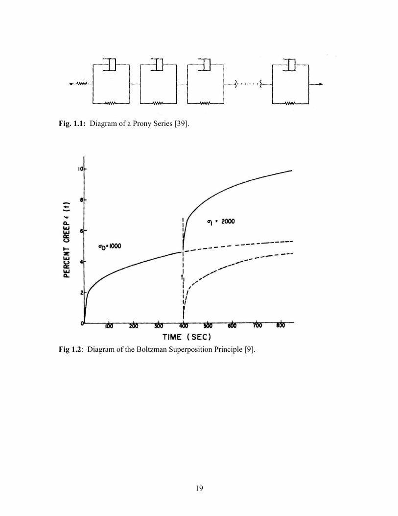
models are mentioned by Flugge [2] as examples. A Prony Series can be described as N

3

Kelvin elements (springs and dashpots in parallel) in series with a lone spring, as shown

in Fig. 1.1. The time dependent compliance of this model can be represented as [3]

∑=

−

−+=

N

r

t

roreDDtD

1

1)( τ (1.2)

where Do and Di, are positive constants, and where τi is the retardation time. The spring-

dashpot models are very versatile in that additional stiffness and damping mechanisms

can model varying modes of viscoelastic response occurring in long duration tests when

compared to the power law model which models only one mode. There are many other

forms of the time dependent compliance used to model viscoelastic behavior which will

be explored in the next section.

Calculation of the time dependent strain response from the known time dependent

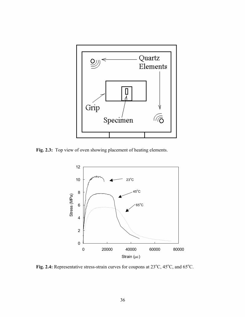
compliance may be accomplished utilizing Schapery’s application of the Boltzmann

superposition principle. This principle indicates that the final stress or strain response of

a material to a series of applied displacement or loads is the summation of all the

individual stress or strain responses to the individual displacement or loads. This can be

graphically represented as in Fig. 1.2. In this figure, a second creep stress is applied at

400 seconds. The strain response (dashed line) from that load, as if it were applied to an

unstressed specimen, can be added to the strain response from the initial stress.

Schapery’s application of this principle has been called the convolution integral and may

be expressed as

τττστε d

ddtDt

t )()()( ∫ ∞−−= (1.3)

where ε(t) is the strain response to an applied load, D(t) is the time dependent compliance

and σ(t) is the applied stress. Eq. (1.4), when used to evaluate the time dependent

4

compliance given by Eq. (1.1) or (1.2) results in a viscoelastic model for the strain

response.

Schapery presents a general form of the time-dependent non-linear compliance,

from which linear compliance may be derived, as

∆+==

σσε

atDggDgtD oo

o21)( (1.4)

where Do is the instantaneous compliance, and ∆D(t) is the time dependent compliance.

(Note that both Eq. (1.1) and (1.2) can be expressed in the form D(t)=Do+∆D1(t).) The

equation is non-linear due to the presence of go, g1, g2 and aσ which are stress dependent

parameters, and are related to the stress dependence of Gibb’s free energy and other free

energy and entropy production concepts. [1] These parameters are not time dependent,

and are therefore evaluated after integration has been completed, as seen in Eq. (1.4) A

linear viscoelastic model results when go=g1=g2=aσ=1, ie. there is no stress dependence.

1.2.2 Viscoelastic models

Walrath [4] utilized a power law model in his exploration of the behavior of the

non-linear strain response of an aramid reinforced epoxy. He incorporated two

viscoelastic constituents into the nonlinear viscoelastic parameters, and found that this

worked reasonably well for predicting uniaxial creep and recovery response of the

composite. He also was able to model temperature dependent strain response using the

time-temperature superposition principle (TTSP) manifested in a time shift factor.

Elahi and Weitsman have used the linear power law compliance model with great

success in modeling the linear viscoelastic strain response and non-linear response of a

random oriented glass fiber/urethane resin composite [5,6]. A damage model with short

5

and long time dependence was utilized to model the behavior above a threshold stress.

Rangaraj and Smith, [7] also utilized a linear power law in their investigation of the creep

and recovery behavior of a WPC with the same volumetric constituency as that utilized in

this work. This was found to model the strain response to an applied load in creep and

recovery reasonably well within stress levels at which damage did not occur (material

stiffness did not change after load application). At stress levels where material

degradation occurred, use of a damage model applied to the power law was found to

account for damage and adequately model strain response. Details of this work will be

described further in Chapter 3.

Sain, et. al [8] utilized a similar power law equation in their investigation of PVC

based, PE based, and PP based wood-plastic composites,

τεε Att o +=)( (1.5)

where A is the amplitude of the transient creep strain, εo is the instantaneous strain and τ

is the time constant. Testing was conducted between 22oC and 60oC. The time constant τ

and the instantaneous strain εo were adjusted with temperature based on empirical data to

account for the temperature dependence of the modeled strain response. Utilizing

flexural testing, they noted the relatively low temperature dependence of the time

dependent portion when compared to the temperature dependence of the instantaneous

strain. However, as greater loads were applied, the time dependent strain became more

influential in the overall flexural creep strain response. It was also noted that the addition

of wood into a PE matrix significantly retarded the time dependent strain response when

compared to the strain response of virgin PE. It was also found that the response of a

6

wood-fiber composite could not be predicted based on a rule of mixtures combination of

the properties of the constituents.

Other investigators have utilized other models to describe the time dependent

response of viscoelastic materials. The Nutting equation mentioned by Neilsen and

Landel [9] has been used to describe the uniaxial strain response of a viscoelastic

material. It can be expressed as

ntKt βσε =)( (1.6)

where K, β and n are constants at a given temperature, and β is equal to or greater than 1.

While this equation models experimental data reasonably well in the linear region where

β=1, however n has been observed to change over long times. A hyperbolic tangent

function has been used to model the non-linear stress-strain response of a wood plastic

composite by Hermanson, et. al. This can be described as

)tanh( εσ ba= (1.7)

where a and b are parameters to fit the experimental data, [10] and are analogous to

strength and modulus. This method is mostly empirical and does not describe time

dependence. Conversely, the hyperbolic sine function has been validated by Neilsen, [11]

among others. The hyperbolic sine function can be represented

c

tKtσσε sinh)()( = (1.8)

where K(t) defines the creep time dependence and σc is a critical stress. However, σc

varies with temperature and material structure. [8] A hyperbolic sine function has also

been ulitized to describe the stress dependence of the go and g1g2/aσ terms in Eq. (1.4) by

Schapery [1] and Van Holde[12].

7

Veazie and Gates, [13] in their study of the aging of an aerospace composite,

utilized a linear viscoelastic creep compliance of the form

βτ )/(0)( teStS = (1.9)

where S0,τ and β are the initial compliance, retardation time, and shape parameter

respectively. While they indicate that this equation reaches its limitations at very large

times, they did not approach the limits of this function in their testing to 108 seconds of

shifted time. An additional time shift factor was used to account for aging.

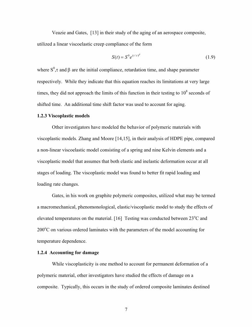
1.2.3 Viscoplastic models

Other investigators have modeled the behavior of polymeric materials with

viscoplastic models. Zhang and Moore [14,15], in their analysis of HDPE pipe, compared

a non-linear viscoelastic model consisting of a spring and nine Kelvin elements and a

viscoplastic model that assumes that both elastic and inelastic deformation occur at all

stages of loading. The viscoplastic model was found to better fit rapid loading and

loading rate changes.

Gates, in his work on graphite polymeric composites, utilized what may be termed

a macromechanical, phenomonological, elastic/viscoplastic model to study the effects of

elevated temperatures on the material. [16] Testing was conducted between 23oC and

200oC on various ordered laminates with the parameters of the model accounting for

temperature dependence.

1.2.4 Accounting for damage

While viscoplasticity is one method to account for permanent deformation of a

polymeric material, other investigators have studied the effects of damage on a

composite. Typically, this occurs in the study of ordered composite laminates destined

8

for aerospace applications. Of primary concern is the understanding of crack propagation

through composite materials, delamination, and the relation of crack density to applied

load. These may be pursued in either a micromechanics fashion, where the effect of the

damage is considered based on crack geometry, or a continuum mechanics fashion, where

damage is defined as a continuous field, and individual crack or defect geometry is

ignored. This simplifies the mathematical representation, but does not provide

information on individual defects [17]. It is this latter avenue which is being pursued in

this work. The purpose of this work was not to identify specific micromechanical

structure developments within the composite during loading, but rather to model the

observed behavior based on classical viscoelastic concepts and provide methods to

predict strain response. Elahi and Weistman [5] used a continuum damage model to

predict strain response by including a damage function with slowly varying and rapidly

varying time dependence in their model. This was found to satisfactorily predict the

strain response of a random glass/urethane composite. However, they did not incorporate

temperature into their study of damage.

Rangaraj and Smith, [7] also utilized a damage model which did not identify

individual cracks, crack propagation, or crack growth. In order to model the strain

behavior of the material above the threshold stress where material stiffness degraded after

load application, damage was modeled as a combination of instantaneous damage and

time dependent damage

>−<++= domctst σσω )(1)( (1.10)

9

where s and c are the instantaneous and time dependent damage parameters, m is an

experimentally determined parameter, σd is the threshold stress, and σo is the applied

creep stress.

Rangaraj and Smith defined damage as resulting in a degradation of the material’s

ability to carry a load which could be measured as a change in stiffness. This is

consistent with work by Reifsnider [18] who has observed that stiffness changes indicate

that damage has occurred in such a way that it can be related to changes in residual

strength. Andersons, Limonov and Tamuzs [19] also concur stiffness changes monitored

throughout a test can be used as a measure for the amount of damage which has occurred.

Webb, et. al. disagree. [20] They remark that because stiffness is only measured in one

direction, it does not give a full picture of the damage mechanisms which are occurring

(eg. interlaminar failure, interstitial failure, matrix cracking, fiber breakage). For instance,

matrix cracking in a long fiber unidirectional composite would not significantly affect the

stiffness, which is primarily due to the fibers. Talreja [21] decries the use of “damage”

and “change in stiffness” as synonyms, proposing that “damage” only be used to describe

the actual physical changes negating confusion and discongruous results between two

different researchers with different ideas of “damage.” However, “damage,” even with

this definition, cannot be quantitatively measured, it can only be observed. Lemaitre and

Chaboche [22] suggest that damage be defined based on the concept of effective stress

)1( De −

=σσ (1.11)

where σe is the effective stress and D =1-Ed/E where E is the elastic modulus of an

undamaged specimen and Ed is the elastic modulus of a damaged specimen and D is the

damage. Damage may be defined as a scalar only if the orientation of microcracks and

10

cavities are distributed in all directions. It is this method for quantifying damage which

Rangaraj and Smith [7] used for their study of their WPC. Based on its proficiency in

modeling the WPC in their work, this method of quantifying damage will be continued in

this research.

1.3 Time-Temperature Dependence

The behavior of polymeric materials is dependent on temperature. The time-

temperature superposition principle (TTSP) proposes that temperature effects may be

described by altering the time scale of the viscoelastic response. This means that the

creep data recorded at a reference temperature and shifted according to

)(

*Ta

ttT

= (1.12)

where aT(T) is the time shift factor, can represent the viscoelastic creep at a temperature

T, providing the data is available over a long period of time. Neilsen and Landel describe

two methods of accounting for temperature effects. [9] The first was developed by

Williams, Landel, and Ferry [23] for temperature dependence of the relaxation modulus

of a polymer or composite and is known as the WLF equation which can be expressed as

( )

ref

refT TTc

TTca

−+

−−=

2

1log (1.13)

where c1 and c2 are material dependent constants, T is the temperature at which the shift

factor is desired, Tref is the reference temperature and aT(T) is the time shift factor, or

horizontal shift factor. This was developed for amorphous polymers in the range of Tg to

Tg+100oC from an understanding of viscosity and free volume. Below Tg an Arrhenius

relationship is typically used, which is the second model described by Neilsen and

Landel. [9] This may be expressed as

11

−=

ref

aT TTR

ETa 11exp)( (1.14)

where the universal gas constant R=8.31 J/molK, Ea is the activation energy, Tref is the

reference temperature in Kelvin, and T is the temperature at which the time shift factor is

desired in Kelvin. [24]

For amorphous polymers, a horizontal shift factor as applied in Eq. (1.13) is

sufficient to correctly model temperature dependent response. This can best be

understood by viewing an example in Fig. 1.3. By applying the horizontal shift

according to the curve shown in the inset, in effect shifting time, a master curve

describing the behavior of the material within the tested temperature range relative to the

reference temperature can be created. Upon application of the time shift factor, time

becomes “reduced time,” t*, where time t in the viscoelastic model is replaced by Eq.

(1.12). Materials which only require a horizontal time shift factor in the application of

TTSP were termed “thermo-rheologically simple” by Schwarzl and Staverman refering to

their work on linear viscoelastic behavior. [25] However the TTSP has still been used

with great success for semi-crystalline polymers and crystalline polymers with the

addition of an empirical vertical shift factor to create a master curve. The mechanism

within these materials that results in the vertical shift factor is not completely understood

although it is typically applied above the glass transition temperature. Several different

theories have been provided.

1.4 Polymeric time-temperature behavior

Crissman [26] refers to the vertical shift factor as a “softening factor” in his study

of semi-crystalline high-density polyethylene (HDPE) based on the instantaneous

decrease in stiffness associated with polymeric materials as temperature increases. By

12

using a non-linear model for strain response, then subtracting out the strain due to

plasticity, he was able to create a master curve, using both horizontal and vertical shift

factors.

Elahi and Weitsman, [5,6] in their application of TTSP with their chopped

glass/urethane composite, multiplied their instantaneous compliance term by a

temperature dependent equation to account for the increase in compliance or “softening”

observed as temperature increased. Penn [27] explains the need for a vertical shift factor

in his examination of HDPE between –20oC and 80oC as softening or premelting of

crystal boundaries.

Onogi, et. al., [28] utilized such methods as Differential Scanning Calorimetry,

Depolarized Light Intensity, Infrared Dichroism, Nuclear Magnetic Resonance, and

Dynamic Mechanical Analysis in their study of thin HDPE films 100-120µm thick.

While the vertical shift factor had been thought to be a representation of the change in

crystallinity, they found that crystallinity did not change with temperature until nearly

105oC. Fukui et. al. [29] also did not observe crystallinity changes until around this

temperature in their rheological investigation of the same material. Further investigation

by Onogi et. al. found that the vertical shift factors required to construct master curves

from the strain optical coefficient and the stress relaxation data obtained through rheo-

optical and mechanical measurements were closely related to the rotation of the

crystallites within the HDPE as temperature increases. Rotation or untwisting of the

HDPE lamellae was also observed as temperature increased. However, they did not rule

out Penn’s conclusions, saying that softening or premelting of crystal boundaries could

also play a role in the vertical shift factor.

13

The usage of a vertical and horizontal shift factors have also been applied to the

physical aging of HDPE. Lai and Bakker [3] argued that the TTSP is generally not

applicable to semi-crystalline polymers owing to the more complex mechanical behavior

between the amorphous and crystalline regions. Additionally, the TTSP cannot be used

to construct the short-term creep compliance master curve of HDPE, in particular, where

aging of the HDPE is involved. However, Lai and Bakker applied a time-stress

superposition principle and utilized a time-stress shift factor in conjunction with a stress

dependent vertical shift factor to construct a master curve for HDPE based on the creep

compliance of differently aged specimens, which suggested that physical aging also shifts

time. This is similar to Schapery’s use of aσ in his development of the time dependent

response of composites in Eq. (1.4). The creep compliance of HDPE was expressed in a

non-linear fashion utilizing a Prony series with 10 terms and was able to satisfactorily

predict the strain response.

In her work, Brinson [30] determined that composites are thermo-rheologically

complex. This would mean that a horizontal shift factor is insufficient to account for

temperature change, and a vertical shift factor would be required to describe the

temperature dependent behavior.

Morgan and Ward [31] in their study of the temperature dependence of the creep

and recovery response of a polypropylene mono-filament also applied a vertical shift

factor to account for changes in the modulus with temperature. They noted that TTSP

applied even for nonlinear materials, where Schwarzl and Staverman only investigated

linear behavior. Both WLF and Arrhenius relationships for the temperature dependence

of the horizontal shift factor were explored within the range of 28oC to 61oC.

14

Much research has been conducted on the time-temperature shift of HDPE due to

its varied and abundant uses, its semi-crystalline morphology, and its complex

viscoelastic behavior. Vertical and horizontal shift factors have been shown to be

required to describe the viscoelastic behavior of HDPE. Vertical and horizontal shift

factors have also been utilized to describe the behavior of other polymers such as

polypropylene, and composites which are deemed thermo-rheologically complex.

1.5 Dynamic Mechanical Analysis

Dynamic Mechanical Analysis (DMA) is often used to determine the viscoelastic

properties of viscoelastic materials. In this method of testing, a sample is either displaced

or loaded at a given frequency in torsion, flexure, or axially. Supposing that a force is

applied at frequency ω, the resulting stress in the material would be

to ωσσ cos= . (1.15)

Due to the inherent vibration damping of viscoelastic materials, the resulting strain would

lag behind the stress by a phase angle δ, which is represented as

)cos( δωεε −= to . (1.16)

This can be seen graphically in Fig. 1.4. This can be represented in the complex form as

"'* iEEE += (1.17)

where E’ is in phase with the strain and is known as the storage modulus for the energy

stored and recovered each cycle. E” is 90o out of phase and is called the loss modulus for

the energy dissipated or lost as heat per cycle. This results in

εσ )"'( iEE += (1.18)

or more succinctly,

15

'"tan

EE

=δ (1.19)

where tan δ is considered the dissipation factor or loss tangent. The viscoelastic data

provided by DMA allows for observation of the effect of temperature on the material

including morphology, relaxation processes, and the time-temperature relationship

(TTSP). Additionally, the effects of frequency on the viscoelastic response of the

material may be observed, as can the physical changes which occur during the curing or

annealing of polymers. [32][33][9]

1.6 Fatigue of composites

The study of fatigue in composites has focussed a significant amount of time and

energy in the analysis of crack growth in composite laminates and aerospace composites.

This may take either a micromechanics approach where the study focuses on the

geometry of the crack and the crack growth phenomenon, or a continuum damage

approach which models the overall change in behavior of the material. Crack growth

studies may include fiber fracture, interstitial fracture, matrix cracking, or delamination.

Other significant fatigue analysis with viscoelastic composites (particularly viscoelastic

polymers) has utilized DMA to record the change in the dynamic properties E’, E” and

tan δ with time, or compared these parameters against frequency or temperature changes.

It is rare to find measurement and modeling of the uniaxial fatigue viscoelastic strain

behavior of composites, and of that, exploration of the relation of that behavior to creep

behavior is minimal. These have been developed in part by Elahi and Weitsman [5,6] and

Scavuzzo [34].

Study of the fatigue failure behavior in uniaxial fatigue loading of HDPE was

conducted by Kaiya, et. al. [35] utilizing DMA. Determination was made of the energy

16

loss to heat generation relationship and the energy used to cause failure. A failure

criterion was established based on the hysteresis loss energy. This was done in strain

controlled tension-compression fatigue with R= -1 where (R=εmin/εmax), pure tension

fatigue with R=0, and pure compression fatigue with R=-∞. In tension compression, or

pure compression, a kink band was formed prior to failure and the failure surface was at

45o to the direction of straining in the maximum shear stress plane. In pure tension

fatigue, the fracture surface was perpendicular to the axis of straining. A study was also

conducted on the fatigue life relative to the strain amplitude in the three loading cases.

Pure compression tests were found to have the longest life for any given strain as the

cracks formed in the kink band were not expanded during loading as was found in the

other cases.

Jo, et al [36] studied the effect of crystallinity compared to annealed HDPE on the

strain controlled fatigue behavior of specimens, utilizing the storage modulus, E’ and the

dissipation factor tan δ. They also defined a “nonlinear viscoelastic parameter” which

described how the stress wave differed from the fundamental stress wave based on the

Fourier series expansion of the response stress. Crystalline HDPE was found to fail more

suddenly without the gradual decrease in E’ that was seen with annealed HDPE. A

sudden increase in their non-linear viscoelastic parameter was observed at the same time

as deformation of spherulites were observed via small angle light scattering, indicating

that their non-linear viscoelastic parameter was a measure of structural changes within

the material.

Xiao [37] studied the effect of hysteretic heating on the fatigue life of an AS-

4/PEEK thermoplastic composite. He developed a way of correlating the hysteretic

17

heating with the thermal degradation of strength and fatigue life of this material, allowing

predictions of fatigue life to be made by knowing the static strength and temperature

relationship and a prediction of the temperature rise due to hysteretic heating.

O’Brien and Reifsnider [38] studied boron/epoxy laminates in strain controlled

fatigue at 30Hz to predict stiffness changes based on fiber breakage or debonding, two of

the several damage mechanisms which composites fail under, using a micromechanics

approach. They found that matrix damage correlated well with stiffness changes in the

material.

Scavuzzo [34] is one of the few researchers who has compared creep and fatigue

loading of any particular material. He studied the behavior of injection molded HDPE

specimens in dynamic and monotonic stress relaxation. Monotonic specimens were

displaced and the stress was recorded over time. For dynamic stress relaxation, the mean

of the cyclic displacement was the same as the monotonic displacement. The amplitude

of the cyclic displacement was a small amount compared to the initial displacement. A

more rapid time-dependent relaxation response was observed for coupons subjected to

cyclic displacement than was observed in specimens subjected to a constant initial

displacement.

Elahi and Weitsman [5,6] studied the response of the glass/urethane composite in

uniaxial fatigue loading up to 2000 cycles utilizing a sawtooth loading function, which

allowed for a summation of the strain response to each loading and unloading cycle. This

greatly simplified the evaluation of the integral representation of the strain behavior in

the power law form. Good results were obtained with all applied stresses except where

coupon failure occurred due to lack of a failure criterion in this model. This is unique

18

among the literature surveyed as Elahi and Weitsman are the only researchers found

which have applied classical viscoelasticity to model the strain response of a uniaxial

fatigue specimen. While they had incorporated temperature dependence in creep loading

of this same material, they did not examine how temperature changes affect fatigue

loading.

1.7 Summary

The viscoelastic behavior of composites and polymeric materials can be modeled

using significantly different approaches. These may be developed with concepts of

mechanics or may be purely an empirical fit. Different studies have found different

models which will satisfactorily describe the viscoelastic behavior of the same material,

however, some models work better than others. HDPE is itself a unique material to model

as understanding of the semi-crystalline nature is still developing, as can be seen by some

of the differing opinions on the morphology occurring across temperature ranges and

mechanical loading. Previous work concerning the viscoelastic behavior of the WPC

studied herein considered only creep/recovery response up to 1000 minutes with a power

law model. Using the TTSP, studies at elevated temperatures will increase the

knowledge of the behavior by four orders of magnitude utilizing a prony series model,

and will provide an understanding of the effects of temperature on the viscoelastic

behavior of the material. Further, while monotonic and cyclic uniaxial loading have been

studied separately, it is rare that they are studied together, and rarer yet that a cohesive

model is attempted to describe both behaviors. This work will go beyond that to apply a

creep model to fatigue loading, including accounting for temperature dependence and

damage.

19

Fig. 1.1: Diagram of a Prony Series [39].

Fig 1.2: Diagram of the Boltzman Superposition Principle [9].

20

Fig. 1.3: Time-Temperature Superposition applied to the stress relaxation of a hypothetical polymer. The master curve shown is made by applying horizontal shifts in accordance with the plot of shift factors aT against time shown in the inset. [9]

Fig 1.4: Relationships between stress, strain and resulting phase angle and storage and loss modulus and phase angle utilized during DMA analysis. [32].

21

REFERENCES

[1] Schapery, R.A., On the Characterization of Nonlinear Viscoelastic Materials, Polymer Engineering and Science, Vol 9:4, July 1969. [2] Flugge Wilhelm, Viscoelasticity, Springer-Verlag, 1975. [3] Lai, J., Bakker, A., Analysis of the non-linear creep of high density polyethylene, Polymer, Vol 36, No 1, 1995. [4] Walrath, David E., Visceolastic Response of a Unidirectional Composite Containing Two Viscoelastic Constituents, Experimental Mechanics, June 1991. [5] Elahi, M., and Weitsman, Y.J., On the Mechanical response of P4 Chopped Glass/Urethane Resin Composite: Data and Model, Oak Ridge National Laboratory, ORNL –6955, October, 1999. [6] Elahi, M., and Weitsman, Y.J., Some aspects of the Deformation Response of Swirl-Mat Composites, Oak Ridge National Laboratories, ORNL/TM-13521. [7] Rangaraj, Sudarshan V., and Smith, Lloyd V., The Nonlinear Viscoelastic Response of a Wood-Thermoplastic Composite, Mechanics of Time Dependent Materials, 3:125-139, 1999. [8] Sain, M.M., Balatinecz, J., and Law, S., Creep Fatigue in Engineered Wood Fiber and Plastic Compositions, Journal of Applied Polymer Science, Vol. 77, pp.260-268, 2000. [9] Nielsen, Lawrence F., Landel, Robert F., Mechanical Properties of Polymers and Composites 2nd edition, Marcel Dekker, 1994. [10] Hermanson, John C., Adcock, Timothy, and Wolcott, Michael P., Section Design of Wood Plastic Composites, under contract No. 00014-97-C-0395, quarterly report May 27, 1999. [11] Nielsen, Lawrence E., The Stress Dependent Creep of Polyethylenes, Journal of Applied Polymer Science, Vol. 13, pp 1800-1801, 1969. [12] Van Holde, Kensal, A Study of the Creep of Nitrocellulose, Journal of Polymer Science, Vol. 24, pp 417-427, 1957. [13] Veazie, David R. and Gates Thomas S., Tensile and Compressive Creep of a Thermoplastic Polymer and the Effects of Physical Aging on the Composite Time-Dependent Behavior, ASTM Special Technical Publication: Time Dependent and Nonlinear Effects in Polymers and Composites, n 1357 2000, pp160-175.

22

[14] Zhang, Chuntao, and Moore, Ian D., Nonlinear Mechanical Response of High Density Polyethylene. Part 1: Experimental Investigation and Model Evaluation, Polymer Engineering and Science, Vol 37 No 2, Feb 1997, pp404-413. [15] Zhang, Chuntao, and Moore, Ian D., Nonlinear Mechanical Response of High Density Polyethylene; Part II, Uniaxial Constuitive Modeling, Polymer Engineering and Science, Vol. 37 No 2, Feb 1997, pp444-420. [16] Gates, Thomas S., Effects of Elevated Temperature on the Viscoplastic Modeling of Graphite/Polymeric Composites, ASTM STP 1174, American Society for Testing and Materials, Philadelphia, 1993, pp201-221. [17] Hashin, Z, Micromechanics Aspects of Damage in Composite Materials, Durability of polymer based composite systems for structural applications, London, Elsevier Applied Science, 1991. [18] Reifsnider, Kenneth L., Damage Mechanisms in Fatigue of Composite Materials, Fatigue and Creep of Composite Materials, Proceedings of Symposium, Riso National Laboratory, 1982. [19] Andersons, J., Limonov, V, Tamuzs, V., Fatigue of Polymer composite materials, Institute of Polymer mechanics Riga Latvia, Durability of polymer based composite systems for structural applications, Cardon A.H., and Verchery G., editors, London: Elsevier Applied Science, 1991. [20] Webb, G.T., Breunig, T., Stock, S.R., Antolovich, S.D., Damage Accumulation in Metal Matrix Composites during fatigue with emphasis on B/Al and SiC/Al, Memoires et Etudes Scientifiques Revue de Metallurgie, October, 1990. [21] Talreja, Ramesh, Damage mechanics of Composite materials based on Thermodynamics with internal variables, Durability of polymer based composite systems for structural applications, Cardon, A.H., and Verchey, G., editors, Elsevier Applied Science, London, 1991. [22] Lemaitre, Jean, and Chaboche, Jean-Louis, Mechanics of Solid Materials, Cambridge University Press, 1990. [23] Williams, M.L., Landel, R.F., and Ferry, J.D., Journal of the American Chemical Society, 77, 3701, 1955. [24] McCrum, N.G., Buckley, C.P., Bucknall, C.B., Principles of Polymer Engineering, Oxford University Press, New York, 1988. [25] Schwarzl, F. and Staverman, A.J., Time-Temperature Dependence of Linear Viscoelastic Behavior, Journal of Applied Physics, Vol. 23 No 8, Aug 1952.

23

[26] Crissman, J.M., Creep and Recovery Behavior of a Linear High Density Polyethylene and an Ethylene-Hexene Copolymer in the Region of Small Uniaxial Deformations, Polymer Engineering and Science, 26: n15, 1986. [27] Penn, Robert W.,Dynamic Mechanical Properties of Crystalline, Linear Polyethylene, Journal of Polymer Science: Part A-2, 4: 545-557 1966. [28] Onogi, S., Sato, T., Asada, T, and Fukui, Y., Rheo-Optical Studies of High Polymers, XVIII. Significance of the Vertical Shift in the Time Temperature Superposition of RheoOptical and Viscoelastic Properties, Journal of Polymer Science: Part A-2 Vol 8, 1211-1255, 1970. [29] Fukui, Y., Sato, T., Ushirokawa, M., Asada, T, and Onogi, S., Rheo-Optical Studies of High Polymers. XVII. Time-Temperature Superposition of Time-Dependent Birefringence for High-Density Polyethylene, Journal of Polymer Science: Part A-2, Vol 8, 1195-1209, 1970. [30] Brinson, L.C., Time-Temperature Response of Multi-phase Viscoelastic Solids through Numerical Analysis, PhD thesis, California Institute of Technology, Feb 1990. [31] Morgan, C.J., Ward, I.M., The Temperature Dependence of Non-linear Creeep and Recovery in Oriented Polypropylene, Journal of the Mechanics and Physics of Solids, Vol 19, pp165-178, 1971. [32] Findley, William N, Lai, James S., and Onaran, Kasif, Creep and Relaxation of Nonlinear Viscoelastic Materials, North Holland Publishing Company, Amsterdam , 1976. [33] Ferry, John D., Viscoelastic Properties of Polymers, John Wiley and Sons Inc., New York, 1980. [34] Scavuzzo, Rudolph J., Oscillating Stress on Viscoelastic Behavior of Thermoplastic Polymers, Journal of Pressure Vessel Technology, Vol. 122, August 2000. [35] Kaiya, Norihiro, Takahara, Atsushi, Kajiyama, Fatigue Fracture Behavior of Solid-State Extruded High-Density, Polymer Journal, Vol. 21 No. 7 pp 523-531 1989. [36] Jo, Nam-ju, Takahara, Atsushi, Kajiyama, Tisato, Analsysis of Fatigue Behavior of High-Density Polyethylene Based on Nonlinear Viscoelastic Measurement under Cyclic Fatigue, Polymer Journal, vol. 25, no. 7, pp 721-729, 1993. [37] Xiao, X.R., Modeling of Load Frequency Effect on Fatigue Life of Thermoplastic Composites, Journal of Composite Materials, Vol. 33, No. 12/1999.

24

[38] O’Brien, T.K. and Reifsnider, K.L., Fatigue Damage: Stiffness/Strength Comparisons for Composite Materials, Journal of Testing and Evaluation, Vol. 5, No. 5, September 1977. [39] Gibson, Ronald F., Principles of Composite Material Mechanics, McGraw-Hill Inc., 1994.

25

CHAPTER TWO

MATERIALS AND TESTING

2.1 Introduction

The material utilized in this study is not commercially available. Therefore, the

method of manufacture and material constituency will be described. Further, the

specimen geometry is described, as are the methods used to characterize the material.

Experimental methods used for comparison with the model are also described along with

material properties and descriptions of the variation within the material.

2.2 Material Processing

The wood plastic composite under investigation in this research had a

composition by weight of 58% dried maple flour, 31% HDPE matrix, 8% talc, 2% zinc

stearate, and 1% wax. The constituents were mixed dry in a drum blender then extruded

through a twin screw counter-rotating extruder. During the extrusion process, the dry

constituents were fed into the barrel where the mixture was heated with a barrel

temperature of 163oC (325oF) and compressed while driven toward the end of the barrel

and the die. Before entering the die, the melt was forced through a screen pack and the

cross sectional area of the melt was reduced. The melt was then forced through the die

which was maintained at 171oC (340oF). Upon exit from the die, the 152mm wide by

13mm thick extrusion was cooled with ~15oC (50oF) tap water. A schematic of the

extrusion process may be seen in Fig. 2.1 where a single screw extruder is shown.

This board was cut into 200mm (8 inch) long sections then cut into coupons

25mm (1 inch) wide or 32 mm (1-1/4 inches) wide. The 25 mm wide coupons were used

26

for creep and bending testing, while the 32mm wide coupons were dogboned to a 25mm

wide gage section for fatigue and tensile strength testing to prevent specimen failure at

the grips during testing. Coupons were marked to facilitate consistent positioning within

the grips and of the extensometer. During loading of the coupons, 41 mm (1.625 inches)

were clamped in each grip, and the remaining 121 mm (4.75 inches) was stressed. The

extensometer was positioned directly between the grips.

2.3 Testing Methodology

2.3.1 Testing Equipment

Experiments were conducted on a 2-post servohydraulic load frame with a 45kN

(10 kip) load cell. The load frame was controlled with an MTS 407 Controller. Strain

was measured with an MTS 634.11E-24 extensometer with a 25 mm (1 in.) gage length.

It was then conditioned with a Vishay 2120A strain conditioner and filtered through a

low pass filter, which reduced extensometer noise from 70-80µε to 5-7µε as shown in

Fig. 2.2. This was required due to the low magnitude of the strains considered in this

research in calculating stiffnesses and verifying viscoelastic behavior. The extensometer

was aligned to the edge of the coupon with an aluminum block designed to minimize

experimental error due to misalignment. Also utilized for room temperature testing was a

4-post servohydraulic load frame with a 90kN (20kip) load cell. Control and strain

measurement was achieved using the same equipment as for the 2-post load frame.

The 2-post load frame was equipped with an oven to facilitate measurements

above room temperature. The oven was constructed of 38mm (1-1/2 inch) foil-covered

foam insulation board. This was fitted around the grips to prevent significant thermal

losses due to airflow through gaps. The interior dimensions were 36 cm (14 in.) in all

27

directions. Heating was provided by two 300-watt quartz heating elements, located

across the diagonal of the oven as shown in Fig. 2.3. An Omega CN9000A controller

was used to control oven temperature via a K-type thermocouple attached to the surface

of the coupon. The thermocouple was fixed slightly below the extensometer with high

temperature tape. In order to determine the soak time necessary for the temperature of

the coupon to reach steady state in the oven, a blind hole was drilled in a coupon into

which the thermocouple was inserted. Interior coupon temperature was found to reach

equilibrium with the surface of the coupon within 15 minutes. In order to ensure that

steady state was reached in the testing portion of this work, coupons were placed in the

oven for several hours prior to testing, and were allowed 30 minutes to reach temperature

after they had been loaded in the top grip. Data was recorded using customized Labview

software.

2.3.2 Quasi-static Loading

For all loading scenarios, coupons were first placed in the top grip. The

extensometer was attached and zeroed, the bottom grip was then closed. Due to coupon

warpage or slight grip misalignment, initial strains were observed when the bottom grip

was closed on the coupon at zero load. Therefore, the initial strain at zero load was

recorded and used to adjust measured strain output during analysis of raw data. In

quasi-static loading, coupons were elongated in displacement control at 1.3 mm/min

(0.050 in./min). Time, load, stroke and strain data were recorded with customized

Labview software. Engineering stress was calculated based on the initial cross-sectional

area of the coupon. A sample stress-strain curve for a coupon at each temperature is

shown in Fig. 2.4.

28

Material stiffness was measured as a chord modulus between 0.7 MPa (100psi)

and 3.2 MPa (230psi or 30% Sut) at room temperature. This stress was below what is

termed the “threshold stress” above which permanent deformation and stiffness change

occurred. Use of this range allowed for a consistent zone of measurement regardless of

the stress level the coupon was being loaded to. This is similar to the range used by

Rangaraj [1] in his measurement of elastic modulus for his WPC. Rangaraj had used a

chord modulus during the unloading portion of the creep/recovery test over the same

stress range at which initial stiffness was measured during loading to determine changes

in the stiffness of the coupon during the creep test. Experimental application of this

method proved inconsistent in practice. For this reason, the elastic modulus was

measured well after recovery, (approximately 30to) during a ramp load and immediate

unload at room temperature over the same range as initial stiffness was measured to

determine stiffness change.

2.3.3 Creep Loading

A schematic of a typical creep test is shown in Fig. 2.5. A creep load is applied at

t=0 for a time t=to at which time the load is instantaneously removed. Ideally, creep

coupons would be loaded and unloaded instantaneously. However, this cannot be

achieved in practice. Coupons were therefore loaded at a ramp rate of 200N/sec (45

lb/sec) then held at a load for a determined amount of time, 0, 10, or 1000min. For

recovery, load on the coupon was removed at the same rate at which it was applied.

When near zero load was reached, the bottom grip was opened, completely unloading the

coupon. The coupon was then allowed to recover for three times the creep duration (3to)

during which strain was recorded. Loading was accomplished in 4-17 seconds depending

29

on the creep load level. This was found to be a favorable load application rate in work by

Rangaraj [1], being rapid enough to have negligible effect on the creep outcome, and not

being too rapid so as to damage the coupon by imparting inertia effects to the

specimen.[2] LabView software was utilized to record load, stroke and strain data at user

controlled periods. A test matrix for creep loading may be seen in Table 2.1.

Table 2.1: Test matrix for creep and recovery tests. Entries in the table indicate the number of test replicates.

Sut 30% 50% 70% 90% Creep

Duration (min)

0

10

1000

0

10

1000

0

10

1000

0

10

1000

23oC 5 5 3 5 5 3 5 5 3 5 2 0

45oC 0 5 1 0 3 1 5 5 3 0 2 0

65oC 0 3 1 0 3 1 5 5 3 0 4 0

The strain during the unloading phase was not adjusted as described in the previous

section as the grip-induced strain was nonexistent as the bottom grip was open during

recovery.

2.3.4 Fatigue Loading

Fatigue loading was likewise accomplished in load control. Coupons were loaded

with R=.1 (R=σmin/σmax) in all stress levels tested. Experimental strain measurements

recorded with the extensometer over the range from 0.1Hz to 30Hz were found to be the

most accurate at lower frequencies where extensometer slip was less likely to occur.

Fatigue life and hysteretic heating were observed to decrease with load frequency (to be

discussed in section 2.4.2). A frequency of 0.5Hz was therefore chosen for subsequent

fatigue tests reported in this work. Experimental peak cyclic strain was recorded at

30

intervals throughout the tests utilizing customized LabView software. To evaluate the

viscoelastic response of the WPC at various temperatures and stresses, three coupons

were tested at each stress level and temperature: 30% and 70%Sut at 23oC, 45oC, and

65oC for 100 minutes. Several coupons were also tested for longer durations at 30% and

70% to better evaluate the model over long times. Initial and final elastic moduli were

recorded to determine the fatigue induced damage.

2.3.5 Dynamic Mechanical Analysis

Dynamic Mechanical Analysis (DMA) was utilized to determine time temperature

shift factors. Analysis was conducted on a Rheometrics Solid Analyzer (RSA II).

Specimens were machined from the center of straight coupons to eliminate edge effects,

saw marks, and possible damage due to the circular saw cutting of the coupons.

Specimens were machined on a Bridgeport milling machine using a fly cutter and an

endmill for finish cuts to achieve good surface finish on the specimen, minimizing

surface imperfections which could have caused stress concentrations affecting the results.

Specimen dimensions were 45 mm long, 6 mm wide, and 2 mm thick. These were

loaded into a dual cantilever fixture. A flexural strain of 3.0x10-5 was applied at

frequencies between .01Hz and 10 Hz in a frequency sweep at each temperature. Data

was recorded at 5 frequencies within each decade. A frequency sweep was conducted

every 2oC from –30oC to 65oC. Initial soak time to reach –30oC was 10 minutes. Soak

time associated with each 2oC temperature jump was 1 minute.

31

2.4 Results

2.4.1 Material Characterization

Quasi-static tests were conducted to determine baseline material properties for the

formulation. The dependence of material properties on the location across the width and

along the length of the extruded board was also investigated. No location dependence

was discovered in the coupons along the length of the boards. However, variations in

stiffness and ultimate strength were discovered across the width of the board as shown in

Fig. 2.6. Strength was on the order of 10% higher in the coupons taken from the outside

edge of the board than in the coupons cut from the interior of the board. Stiffness was

nearly 20% higher at the outside of the board. These increases were expected given the

3-dimensional cone-shaped reduction of the die area as the material was extruded, which

resulted in greater compression of the extruded material near the edges of the die. In

order to minimize variation in the properties of dogboned and straight coupons used for

the other experiments covered in this work, the outer 20mm were discarded from each

edge of the board prior to cutting the coupons. The effect of coupon geometry can also

be observed in Fig. 2.6. Dogboning of coupons had a negligible effect on the measured

stiffness, and a beneficial effect on measured strength.

To consider the effect of temperature on coupon strength, seven coupons were

loaded at 23oC, 45oC, and 65.5oC (73, 110, and 150oF). The strength and elastic modulus

were recorded and plotted. Both strength and elastic modulus decreased in a nearly linear

fashion with temperature as can be seen from Fig. 2.7. Strength at 65.5oC was nearly half

that at 23oC. Normalization of the strength and elastic modulus with the reference

strength and elastic modulus at 23oC is shown in Fig. 2.8. Note that the rates of change

32

of strength and elastic modulus are not identical but are similar. Further, material

toughness increased by a factor of three at 65oC relative to material toughness at 23oC. A

comparison of the stress-strain response of the WPC at 23, 45 and 65oC is shown in Fig.

2.4.

In order to compare the responses of coupons loaded at different temperatures in

creep and fatigue, the percentages of ultimate strength used to denote the loading of the

coupon were normalized with the ultimate strength at each temperature as shown in

Table 2.2. Thus, for example, a coupon loaded in creep at 30% Sut at 23oC was loaded

to 3.2MPa, while a coupon loaded at 30% Sut at 65oC was loaded to 1.7MPa.

Table 2.2: Normalization with respect to temperature dependent ultimate strength (Sut). 30% Sut 50% Sut 70% Sut 90% Sut 100% Sut

Temp (oC) (MPa) (MPa) (MPa) (MPa) (MPa) 23 3.2 5.4 7.5 9.7 10.7

45 2.4 4.0 5.6 7.3 8.1

65 1.7 2.8 3.9 5.0 5.5

2.4.2 Fatigue

It is known that HDPE is rate dependent; therefore, initial trials were conducted to

determine the effects of loading frequency on the fatigue life of the coupons. The

coupons were loaded with σmax = 80% Sut of the wood-plastic material. A thermocouple

was attached to the coupon in order to monitor temperature change during the test.

Testing was conducted at frequencies of 0.09 Hz, 0.5 Hz, 5Hz, and 30 Hz. Five coupons

were tested at each frequency. As can be seen in Fig 2.9, fatigue life increased with

loading frequency. This is consistent with work published by Xiao [3] who noted that

when the rise in temperature due to hysteretic heating is not significant, fatigue life will

33

increase with load frequency. This has been found to be true with graphite/epoxy and

boron/epoxy composites. However, with composites such as glass/epoxy and an AS4-

PEEK thermoplastic composite, which are known to exhibit high hysteretic heating, the

opposite occurred. Temperature rise was observed in AS4-PEEK in all load frequencies

from 1Hz to 10Hz and increased as frequency increased. In the WPC studied here,

hysteretic heating was only measurable at 30Hz where the temperature increased 15oC

prior to failure. Hysteretic heating was not observed at other frequencies tested. By

contrast, according to Hertzberg and Manson, virgin polyethylene fails in fatigue

primarily by thermal melting, rather than mechanical processes. [4] Other factors not

mentioned by these authors which may also effect the fatigue life could include the

increased duration of load application as frequency decreases, and the stiffness and

strength of the polymer increasing with load rate.

2.4.3 DMA

Analysis of the data by RSA proprietary “Orchestrator” software calculated

specific time shift factors which would result in superposition of the individual relaxation

curves taken at each temperature with respect to the reference temperature of 23oC. (The

relaxation curves showed the variation of E’ vs. frequency (Hz) across a frequency sweep

from 0.1 Hz to 10Hz.) This was done within the software by determining the factor

required to minimize the difference between the reference curve (in this case 23oC) and

the curves from each of the other temperatures numerically. The software then was able

to calculate the constants, c1 and c2, based on the slope and intercept of the plot of (T-

Tref)/logaT versus (T-Tref). Vertical shift factors were excluded in this analysis of the data.

The Arrhenius relationship was determined by solving the Arrhenius equation for the

34

activation energy in terms of the reference temperature, the current temperature, the shift

factor, and the known universal gas constant. The average of the activation energies over

the range from –31oC to 0oC was used since the Arrhenius equation typically describes

the temperature dependence near or below the Tg. A plot showing the shift factors

produced by the DMA analysis, the WLF equation, and the Arrhenius equation for a

representative coupon is shown in Fig. 2.10. As can be seen, the Arrhenius relationship

better describes the shift factors in the lower temperatures than does the WLF equation.

A representative master curve created with the WLF equation for a specimen is shown in

Fig. 2.11.

2.5 Summary

The material properties of the extruded WPC were shown to exhibit some location

dependence across the width of the board. Material property variation was minimized

through selection of coupon location across the board width. Extensometer noise, which

would have been a significant percentage of the strain response in some test cases, was

minimized through electronic filtering. Mechanical testing methods and procedures were

described as well as the procedures used to minimize factors such as ramp loading speed

which could effect experimental results. Further, description was given of the DMA test

equipment utilized for determination of the horizontal shift factor for the WPC.

Frequency effects on fatigue life were observed. As ultimate failure is not an aim

of this work, a relatively low frequency of 0.5 Hz was selected out of experimental

convenience. The material at hand exhibits a strong temperature dependence in stiffness,

strength, and time dependence. The latter appears to be adequately described by TTSP

while the former may be accommodated through concepts of continuum damage.

35

Fig 2.1: Schematic of extrusion process showing a single screw extruder. [5]

Fig. 2.2: Filtered strain response vs. unfiltered strain response.

0

20

40

60

80

100

120

0 2 4 6 8Time (seconds)

Stra

in ( µ

ε)

unfiltered strainfiltered strain

36

Fig. 2.3: Top view of oven showing placement of heating elements.

Fig. 2.4: Representative stress-strain curves for coupons at 23oC, 45oC, and 65oC.

0

2

4

6

8

10

12

0 20000 40000 60000 80000

Strain (µε)

Stre

ss (M

Pa)

23oC

45oC

65oC

37

Fig. 2.5: Schematic of creep recovery test. [6]

38

Fig. 2.6: Location dependence of strength and modulus across width of board.

Fig. 2.7: Temperature dependent strength and elastic modulus.

5

6

7

8

9

10

11

12

0 50 100 150

Location along width (mm)

Stre

ngth

(MPa

)

1.5

2

2.5

3

3.5

4

4.5

5

5.5

6

Stiff

ness

(GPa

)

Strength (straight)Strength (dogboned)Stiffness (straight)Stiffness (dogboned)

0

500

1000

1500

2000

2500

3000

3500

4000

4500

0 20 40 60 80

Temperature (oC)

Mod

ulus

(MPa

)

0

2

4

6

8

10

12

Stre

ngth

(MPa

)

strengthmodulus

39

Fig. 2.8: Normalized strength and elastic modulus with strength and elastic modulus at 23oC.

Fig. 2.9: Dependence of fatigue life on fatigue frequency; R=.1, σmax=80%Sut at 23oC.

0

0.2

0.4

0.6

0.8

1

1.2

10 20 30 40 50 60 70

Temperature (oC)

strengthmodulus

100

1000

10000

100000

0.01 0.1 1 10 100

Frequency (Hz)

Num

ber o

f cyc

les

40

Fig. 2.10: Comparison of experimental DMA, Arrhenius, and WLF time shift factors.

Fig. 2.11: DMA master curve created with WLF shift factors for representative specimen.

1.00E+09

1.00E+10

1E-07 0.0001 0.1 100 100000 1E+08 1E+11

Frequency (Hz)

E' (

Pa)

1.E-071.E-051.E-031.E-011.E+011.E+031.E+051.E+071.E+091.E+111.E+131.E+151.E+171.E+19

-40 -20 0 20 40 60 80

Temperature (oC)

aT

DMAWLFArrhenius

41

REFERENCES

[1] Rangaraj, Sudarshan V., Durability Assessment and Modeling of Wood Thermoplastic Composites, Master’s Thesis, Washington State University, August 1999. [2] Lockett, F.J., Nonlinear Viscoelastic Solids, Academic Press, London, 1972. [3] Xiao, X.R., Modeling of Load Frequency Effect on Fatigue Life of Thermoplastic Composites, Journal of Composite Materials, Vol. 33 No. 12, 1999. [4] Hertzberg, Richard W., and Manson, John A., Fatigue of Engineering Plastics, Academic Press, New York, 1980. [5] Groover, Mikell P., Fundamentals of Modern Manufacturing: Materials, Processes, and Systems, John Wiley and Sons, Inc., New York, 1999. [6] Schapery, R.A., On the Characterization of Nonlinear Viscoelastic Materials, Polymer Engineering and Science, Vol. 9:4, July 1969.

42

CHAPTER THREE

TEMPERATURE DEPENDENT VISCOELASTIC CREEP

3.1 Introduction

Creep and recovery tests were performed according to the methods described in

the previous chapter. This data was then used to develop and evaluate a viscoelastic

model which would describe the behavior of the material at temperatures above room

temperature utilizing the time-temperature superposition principle.

3.2 Power Law Model

3.2.1 Development of power law model

Previous work by Rangaraj [1] and Rangaraj and Smith [2] on the viscoelastic

response of wood-plastic composites utilized Schapery’s convolution integral Eq. (1.1),

to describe the coupon time dependent strain response, repeated here for convenience,

τττστε d

ddtDt

t )()()( ∫ ∞−−= (3.1)

where D(t) is the time-dependent compliance of the material, and where

)()( τστσ Ho= (3.2)

is the applied stress for idealized creep loading with H(t) being the Heaviside step

function. This function controls the instantaneous application of a constant load σo.

Rangaraj utilized a linear power law compliance to model the viscoelastic strain response

below a threshold stress. This can be expressed as

n

o tDDtD 1)( += (3.3)

where Do is the time independent or instantaneous compliance, D1 is the time dependent

compliance, and n is an empirically determined material parameter. Values for these

43

parameters were reported by Rangaraj as 0.22 < Do < .28 GPa-1 (1.51 < Do < 1.95 Msi-1),

D1=0.045 Gpa-1min-n (0.31 Msi-1min-n) and n=0.39. Ranges for parameters were due to

slight material inconsistencies. Evaluation of Eq. (3.1) with (3.2) and (3.3) results in a

predicted strain response of the material in creep loading as

on

o tDDt σε )()( 1+= (3.4)

Creep recovery may be modeled by letting the stress function in Eq. (3.2) equal

)()()( ooor tHH −−= τστστσ (3.5)

where to is the elapsed time when the creep load was removed. Evaluation of Eq. (3.1)

for the recovery strain, εr, results in the following equation for the strain response in

recovery

on

on

r tttDt σε ])([)( 1 −−= . (3.6)

Rangaraj and Smith [2] found that the linear viscoelastic models shown in Eq. (3.4) and

(3.6) adequately described the time dependence of their wood-plastic composite in creep

and recovery as well as in ramp loading scenarios below the threshold stress. Application

of their model to the specimens used in this research required some slight modifications

in the values of the constants to properly model the data. Values for Do were found to be

between 0.23 and 0.33 GPa-1 (1.6 and 2.3 Msi-1) while values for D1 were found to vary

between 0.026 and 0.047GPa-1min-n (0.18 and 0.32 Msi-1min-n). Variation in material

parameters was due to inherent material variation and location dependence of the material

properties across the width of the board. Comparisons of the power law model and

experimental data for a representative coupon is provided in Fig. 3.1.

44

3.2.2 Development of non-linear viscoelastic power law model

In order to model the viscoelastic response above the threshold stress, Rangaraj

[1] utilized a continuum damage model to account for the observed stiffness loss and

permanent deformation observed. Damage, recalling the discussion in Chapter 1, can

have a rather ambiguous definition and may be defined differently depending on the

researcher. Lemaitre and Chaboche [3] suggest that damage be defined based on the

concept of effective stress

)1( De −

=σσ (3.7)

where σe is the effective stress and D =1-Ed/E where E is the elastic modulus of an

undamaged specimen and Ed is the elastic modulus of a damaged specimen. It is this

method for quantifying damage which Rangaraj and Smith [2] used for their study of

their WPC. They reported damage occurring at approximately 5 MPa, or around 45% of

the ultimate strength (Sut) of their WPC. Applying the concept of effective stress to Eq.

(3.1) results in

ττ

τστε d

ddtDt et )()()( ∫ ∞−

−= (3.8)

where the effective stress can be expressed as

)(),()()( tHttt ooe ⋅⋅= σωσσ (3.9)

where σo is the applied stress and ω(σο,τ) is the damage function. The damage function

has components of instantaneous damage and time dependent damage, represented by s

and c respectively and can be described as

>−<++= dom

o ctst σσσω )(1),( (3.10)

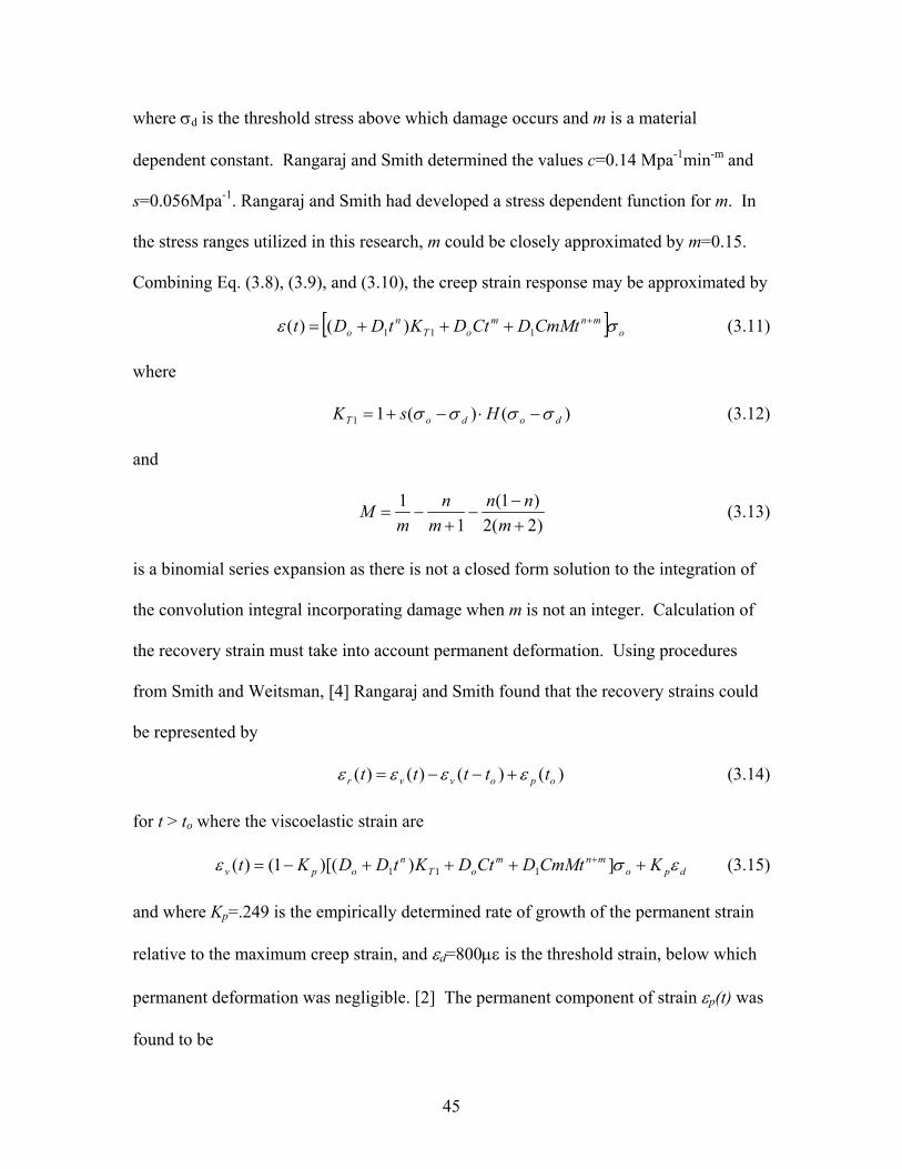
45

where σd is the threshold stress above which damage occurs and m is a material

dependent constant. Rangaraj and Smith determined the values c=0.14 Mpa-1min-m and

s=0.056Mpa-1. Rangaraj and Smith had developed a stress dependent function for m. In

the stress ranges utilized in this research, m could be closely approximated by m=0.15.

Combining Eq. (3.8), (3.9), and (3.10), the creep strain response may be approximated by

[ ] omnm

oTn

o CmMtDCtDKtDDt σε ++++= 111 )()( (3.11)

where

)()(11 dodoT HsK σσσσ −⋅−+= (3.12)

and

)2(2)1(

11

+−

−+

−=m

nnm

nm

M (3.13)

is a binomial series expansion as there is not a closed form solution to the integration of

the convolution integral incorporating damage when m is not an integer. Calculation of

the recovery strain must take into account permanent deformation. Using procedures

from Smith and Weitsman, [4] Rangaraj and Smith found that the recovery strains could

be represented by

)()()()( opovvr ttttt εεεε +−−= (3.14)

for t > to where the viscoelastic strain are

dpomnm

oTn

opv KCmMtDCtDKtDDKt εσε ++++−= + ]))[(1()( 111 (3.15)

and where Kp=.249 is the empirically determined rate of growth of the permanent strain

relative to the maximum creep strain, and εd=800µε is the threshold strain, below which

permanent deformation was negligible. [2] The permanent component of strain εp(t) was

found to be

46

omnm

oTn

opp CmMtDCtDKtDDKt σε ])[()( 111++++= (3.16)

Correlation between this model and a representative coupon loaded for 10 minutes at

70% Sut at 23oC can be seen in Fig 3.2.

3.3 Time-Temperature Superposition

3.3.1 Shifting Time

The time-temperature superposition principle (TTSP) proposes that time and

temperature affect the viscoelastic response of a material in similar ways, and

temperature effects may be described by altering the time scale. This means that the creep

data recorded at a temperature higher than the reference temperature and shifted using the

appropriate shift factor,

)(

*Ta

ttT

= (3.17)

will represent the viscoelastic creep at the reference temperature where aT(T)=1 at an

extended period of time. Time scaling is presented visually in Fig. 1.3 which shows the

application of the time shift factor to experimental stress relaxation data. This shift factor

is called the horizontal shift factor or time shift factor because it shifts the creep curve or

stress relaxation curve horizontally with time. The materials for which the TTSP applies

are termed “thermo-rheologically simple”[5]. While Neilsen and Landel have written that

TTSP is typically limited to amorphous polymers, it can also be applied to semi-

crystalline polymers, such as HDPE, if a “vertical shift factor” is also utilized.[6] This

can be expressed as

=

)()(

TatpDt

Toσε (3.18)

47

where p is the vertical shift factor and aT(T) is the horizontal shift factor. This is in

keeping with work by several other authors in both polymers and composites [7, 8, 9, 10,

11,12]. As was mentioned in Chapter One, these materials where a vertical shift factor is

required are termed “thermo-rheologically complex.” [13]

Two methods are typically used to provide the horizontal or time shift factor for

shifting viscoelastic models. Williams, Landel, and Ferry developed an equation for

temperature dependence of the relaxation modulus of a polymer or composite in what is

known as the WLF equation. [14] This was developed for amorphous polymers in the

range of Tg to Tg+100oC from an understanding of viscosity and free volume. Below Tg

an Arrhenius relationship is typically used, [6] although an Arrhenius relationship can

also be used in regions where the WLF equation would typically apply as an empirical fit

to the shift factor or above where the WLF equation applies.

Penn [9] and Morgan and Ward [12] in their studies of HDPE found that within

temperature ranges that included that studied in this work, there was insufficient

information to determine whether an Arrhenius relationship or a WLF equation was a

better fit. With this in mind, both methods to determine aT were evaluated.

3.3.2 Application to WPC

The WLF equation can be represented as

( )

gg

ggT TTc

TTca

−+

−−=

2

1log (3.19)

where aT is the time shift factor, Tg is the glass transition temperature in Kelvin, and T is

the temperature in Kelvin at which the shift factor is desired. The constants c1g and c2g are

material dependent and have been found experimentally for many polymers. The average

48

values for c1g and c2g for all polymers were determined to be 17.4 and 51.6 respectively.

[15]

The WLF equation (3.19) was developed with Tg as the reference temperature. In

the current work, a reference temperature of 23oC was used. It was therefore necessary to

convert the constants c1g and c2g to reflect a reference temperature of 23oC. Neilsen and

Landel [6] describe the method for adjusting the constants to use a reference temperature

other than the glass transition temperature in the equation. The constants are modified in

the following manner:

grefg

gg

TTccc

c−+

=1

211 (3.20)

grefg TTcc −+= 22 (3.21)

such that the WLF equation becomes

( )

ref

refT TTc

TTca

−+

−−=

2

1~

~~log (3.22)

Because the Tg of the WPC was not known, the Tg for HDPE was an appropriate

place to start. However, uncertainties exist over the glass transition temperature for

HDPE. While values of Tg for HDPE have been reported between –133oC and 67oC in

various sources [16, 17, 18, 19] Sperling reports that the greatest support among

investigators are for Tg’s in three regions: -30oC, -80oC, and -128oC [19]. A Tg of -90oC

was selected as reported by Callister. [16] The constants c1g and c2g for HDPE likewise

are not available in the literature as they are dependent on the elusive Tg, so the

“universal constants” were used. Tabulated values for individual polymers vary only

slightly from the universal constants, so the values used are expected to approximate the

appropriate constants for HDPE. From Eq. (3.20) and (3.21), the constants for a

49

reference temperature of 23oC were found to be 1~c = 6.885 and 2

~c = 164.6oK. Shift

factors determined from Eq. (3.22) will be referred to as “preliminary” since they were

obtained from the universal constants and an observed value of Tg, and will be denoted

with a “~”.

The Arrhenius relationship used to describe the shift factors can be expressed as

−=

ref

aT TTR

ETa 11~exp)(&& (3.23)

where the universal gas constant R=8.31 J/molK, aE~ is the preliminary activation energy

determined from published values, Tref is the reference temperature in Kelvin, and T is the

temperature at which the time shift factor is desired in Kelvin. [20] Published values for

the activation energy for HDPE found to best fit experimental data from thin HDPE films

(100-120µm) and small cylindrical HDPE specimens studied with DMA are between

20.7kcal/mol and 25.2kcal/mol (87kJ/mol and 106kJ/mol). [9,10,11] The average,

aE~ =96.5kJ/mol, was therefore used, and compared with subsequent experimental data.

The shift factors obtained from published values of the activation energy will also be

referred to as preliminary but will be denoted Ta&& to differentiate it from the shift factors

obtained from the WLF equation. Preliminary activation energies will be denoted with a

“~”.

Elahi and Weitsman, who utilized a power law compliance in their study of glass

fiber/urethane composite, showed that the time shift factor aT can be determined

empirically. The log of the time shift factor found experimentally was plotted with

respect to temperature and a polynomial curve fit was used to find an equation describing

aT over the temperature range desired. In order to account for matrix softening, they also

50

plotted the change in the instantaneous compliance Do and using a polynomial fit, found

an equation for F(T)=Do(T)/Do, the instantaneous temperature shift factor (ie. vertical

shift). [7] These shift factors were incorporated into the viscoelastic model used for the

WPC at 23oC given by Eq. (3.4) and Eq. (3.6) which, when evaluated, produced

o

n

To Ta

tDTFDTt σε ])(~)([),( 1

+= (3.24)

and

o

n

T

o

n

Tr Ta

ttTa

tDTt σε ])(~)(~[),( 1

−−

= . (3.25)

This model appeared to be an appropriate model, as previous research by Brinson had

concluded that all composites behave as thermo-rheologically complex materials,

therefore required both a horizontal and vertical shift factors.[13] Experimental

verification of this model was therefore attempted.

3.3.3 Vertical and horizontal shifting

To empirically determine the time shift factor for this material, four coupons were

loaded in creep to 2.03 MPa (300psi) at 23oC (20% Sut), 43oC (26% Sut), and 65oC (37%

Sut) for 10 minutes and allowed to recover. A stress of 2.03 MPa was used because it did

not produce an appreciable change in the measured stiffness in any of the temperature

ranges. The time shift factor aT, and the instantaneous compliance shift factor F(T) were

empirically chosen to fit Eq. (3.24) and Eq. (3.25) to the strain response of each coupon

[7]. The values of Ta~ found experimentally are compared with the horizontal shift factors

calculated using 1~c and 2

~c in Eq. (3.22) and with aE~ from Eq. (3.23), as is shown in Fig.

3.3. Given the preliminary Ta~ from experimental data, as well as knowing Tref, T, and R,

51

a value for aE~ was calculated to best fit the experimental data. This resulted

in aE~ =64.2kJ/mol which fit the data well. Very good correlation between the empirical

data and the predictions from the WLF equation were obtained.

The values of the instantaneous shift factor F(T) are shown in Fig. 3.4, which

suggested a linear dependence with temperature. A linear relationship was also consistent

with the nearly linear dependence of stiffness on temperature, as shown in Fig. 2.8. The

linear equation for the instantaneous stiffness shift factor as a function of temperature T

was found to be

050.120041.)( −= TTF (3.26)

Using the WLF equation described above, a comparison between a representative

coupon and the predicted strain response from Eq. (3.24) and Eq. (3.25), at σo=37% Sut

and T= 65oC is shown in Fig. 3.5. The model appears to capture the creep and recovery

response of the coupon reasonably well. While the prediction of Eq. (3.24) is slightly

above the experiment in this case, it was within the observed experimental scatter of the

WPC.

3.4 DMA

3.4.1 DMA shift factor development

In order to verify the shift factors found from creep testing, five randomly

selected samples machined from untested coupons were analyzed using Dynamic

Mechanical Analysis (DMA). It was found that a master curve could be developed for

each specimen tested utilizing only a horizontal shift factor as can be seen in Fig. 3.6.

This implied that the WPC is “thermo-rheologically simple” instead of “thermo-

rheologically complex” as had been presumed in the development of Eq. (3.24) and

52

(3.25). The constants of the WLF equation were calculated by the RSA II software as a

best fit over the range of –31oC to 65oC for each specimen tested as was described in

section 2.4.3. Averages were taken of the WLF constants c1 and c2 of the 5 specimens to

determine the WLF equation governing this material. The average values of c1 and c2

were 20.534 and 128.78oK respectively. The WLF equation with the DMA developed

constants was a good fit to the experimental data over -10oC-65oC.

The activation energy (Ea) for the Arrhenius equation was calculated by solving

Eq. (3.23) for Ea then calculating Ea from the aT calculated by the DMA software for

each temperature and the known values of T, Tref (23oC), and R. An average of the

experimental shift factors for the four coupons tested between -31oC and 0oC was

calculated as 325kJ/mol and was found to represent well the experimental determined

shift factors in this region. This can be seen in Fig. 2.11. A comparison of the WLF

equation to the DMA determined shift factors in the range of 23oC to 65oC which is

considered in this work can be seen in Fig. 3.7. The Arrhenius equation is also shown in

this figure.

DMA demonstrated that the WPC could be modeled as a thermo-rheologically

simple material. This more generalized approach to expressing temperature dependence

was therefore pursued.

3.4.2 DMA shift factor verification

While the shifts produced from the DMA analysis resulted in a master curve for

the specimens tested, verification of its applicability to the full size coupons under

uniaxial creep loading was necessary. To accomplish this, these shift factors were

applied to the compliance curves developed from creep strain response of four coupons

53

tested at 23, 45 and 65oC. They were found to form approximately continuous curves, or

master curves. (Time shifting alone used in Eq. (3.24) did not produce a smooth curve.)

The creep compliance master curve created from the average WLF equation from DMA

can be seen in Fig. 3.8 for a representative coupon. A creep compliance master curve

was also attempted using the preliminary horizontal and vertical shifts utilized in Eq.

(3.24). The preliminary shifts are compared with the DMA shift in Fig. 3.8. While Eq.

(3.24) was shown to be a satisfactory preliminary model, it is evident that these shifts do

not conform to the TTSP, otherwise a master curve could have been created.

The time shift factor developed from DMA analysis was applied to the power law

model instead of the preliminary horizontal and vertical shifts applied in Eq. (3.24) and

(3.25). The DMA shifts should provide accurate modeling of the viscoelastic behavior of

the material if the power law model can express creep response for long durations, as the

horizontal shift factor based in TTSP is independent of the viscoelastic model. However,

results from the power law model for a coupon at 65oC using the DMA developed

horizontal shift factor did not correlate with experimental observations, as shown in Fig.

3.9. It is obvious that the time dependence and magnitude of the model do not match the

experimental results.

Calculation of Tg from the WLF equation developed by DMA was undertaken by

working backwards using Eq. (3.20) and (3.21). Because there were three unknowns:

c1g, c2g, and Tg, and only two equations, one constant was approximated. Aklonis and

MacKnight [15] show a table of WLF parameters for various polymers. While c1g and c2g

vary only slightly with temperature, c1g was shown to vary less. For this reason, the

value of c1g was selected as the universal constant for polymers, 17.4. Solving for c2g and

54

Tg produced 79.13oK and 246.3oK (–26.7oC) respectively. This value of Tg was near one

of the accepted glass transition temperatures for HDPE of –30oC.

The WLF equation developed with DMA appears to be a more suitable approach

to describing temperature effects than was the combination of vertical and horizontal shift

factors used initially. Apparently the power law, while adequate for short times at 23oC

up to around 1000 minutes, does not describe the viscoelastic response at extended times

or temperatures using only a horizontal shift. Thus the benefit of using only a horizontal

shift is discounted by the need for a more complicated expression of compliance.

3.5 Prony Series Model

3.5.1 Constant stress

The power law will only describe one mode of viscoelastic behavior. Its inability

to predict the viscoelastic behavior of the WPC at longer times through application of

verified shift factors indicated that there were several modes of time dependent behavior

which occur in the WPC. Lai and Bakker utilized a Prony Series model with great

success in modeling the effects of aging on the viscoelastic behavior of HDPE. [21] A

Prony Series models the viscoelastic behavior as a series of springs and dashpots in

parallel, with a lone spring in series with the parallel combinations of springs and

dashpots (Kelvin elements) as represented in Fig. 3.10. The time dependent compliance

of this model can be represented as

∑=

−

−+=

N

r

t

roreDDtD

1

1)( τ (3.27)

55

where Do and Dr are positive constants, and where τr is the retardation time. Applying

this compliance model to the convolution integral to evaluate the strain response results

in

o

N

r

t

roreDDt σε τ

−+= ∑

=

−

1

1)( (3.28)

for the strain response in creep and

o

N

r

ttt

rrrr

o

eeDt σε ττ

−= ∑

=

−−−

1

)(

)( (3.29)

for the strain response in recovery.

In order to create the Prony Series model for this material, the compliance curves

developed from creep strain response data at 23, 45 and 65oC were plotted against shifted

time using the respective horizontal shift factor described by the WLF equation for each

temperature. A master curve was thus formed for each coupon. Mathcad 7 Professional

(Mathsoft Inc.) utilizing error minimization, was used to produce a least squares fit to the

compliance (i.e. Eq. (3.28) divided by σo) with five Kelvin elements. The resulting

equation was then evaluated through the convolution integral to predict strain response

and applied to other coupons which had undergone various creep loads to verify the

model. Some slight modifications were made to the constants in order to provide a

smooth, best-fit curve. The resulting compliance master curve model is plotted against

the compliance master curves created by the four coupons in Fig. 3.11. The values for

Do, Dr, and τr are shown in Table 3.1.

56

Table 3.1: Coefficients for Prony Series model. r

Dr Gpa-1 (Msi-1)

τr min

0 13.4 (1.94) ∞

1 4.48 (.65) 20

2 6.21(.9) 1000

3 5.52 (.8) 12000

4 7.77 (1.126) 148641

5 12.9 (1.8748) 3000000

It may be observed from Fig. 3.11 that the Prony Series model departs from the

creep response of the material below approximately 5 minutes, and above 107 minutes at

23oC, (which is the equivalent of 104 minutes at 45oC or about 15 minutes at 65oC).

However, the ability of the Prony Series to satisfactorily represent the behavior of the

material for the equivalent of a creep test for 107minutes at 23oC (nearly 7000 days or 19

years) is very significant. The model could readily be extended to consider longer

durations as well as better model the initial 5 minutes if more terms were included in the

series and compared to longer duration tests at elevated temperatures.

3.5.2 Non-linear effects

It was noted that the material exhibited stress dependent behavior, even with the

power law, which was overlooked during previous analysis of this material in which a

linear viscoelastic model was used. The stress dependence of Do and D1 are shown in Fig

3.12. It was apparent that a non-linear viscoelastic model must be used for the Prony

Series. Schapery [22] represents the time-dependent, non-linear compliance as

57

∆+==

σσε

atDggDgttD oo

o21

)()( (3.30)

where Do is the instantaneous compliance, and ∆D(t/aσ) is the time dependent

compliance. It should be noted that application of the non-linear parameters can occur

after the time dependent compliance has been integrated through the convolution integral

since they are constant in time. The non-linear parameters go, g1, g2 and aσ are stress

dependent.

Due to the observed non-linearity in the creep response at all stresses, it was

determined that two of the stress dependent parameters utilized in Schapery’s non-linear

compliance model Eq. (3.30) could account for the non-linearity observed with this

material. This can be applied to the strain response in creep as

or

at

rooreDDgt σε στ

−+= ∑

=

−5

1

1)( (3.31)

where go and aσ are stress dependent parameters. These parameters were empirically fit

to the strain response curves from experimental data in the range of 20% Sut to 43% Sut

at 23oC. Fig. 3.13 shows the dependence of go and aσ on the applied stress and can be

described by

8225.0816.)( += oog σσ (3.32)

8555.1248.)( +−= oa σσσ (3.33)

where σo is in MPa. While some material scatter is apparent in Fig. 3.13, a linear stress

dependence was found to satisfactorily model the non-linear behavior utilizing Eq. (3.31).

(Eq. (3.32) and (3.33) had r2 values of .78 and .56 respectively. Above 43% Sut, the

relationships between stress and the values of go and aσ changed significantly. This is

58

likely a result of damage formation as observed from Eq. (3.10). This will be discussed

further in the following section.

Observation of the effects of damage discussed in section 3.2.2 indicates that the

threshold stress for this material was between 43% and 50% Sut. The non-linear model,

Eq. (3.31), was therefore not used above 43% Sut. Fig. 3.14, 3.15, and 3.16 compare the

model to the experimental strain response for representative coupons at various stress

levels and temperatures. As the lower grip is released during the unloading of the

coupons, an impulse can be caused in the coupon. This impulse caused extensometer

slippage, resulting in the recovery offset seen in Fig 3.14 and 3.16. Other deviation from

the model seen in these figures is within the observed inherent variability of the material.

The failure to capture the initial 5 minutes or so of the creep model in Fig. 3.14 is

due to limitations of the Prony Series developed from the master curve. This can be seen

in Fig. 3.12 and was discussed previously. However, the model quickly matches the time

dependent portion of the curve after the initial 5 minutes. Similarly, the initial portion of

the unloading strain response is not predicted during the recovery portion of the model.

However, at temperatures above 23oC, due to the shifted time, the model does describe

the initial strains well. Long-term creep tests of 1000 minutes at room temperature are

also well modeled, as shown in Fig 3.17.

3.5.3 Threshold stress

Previous work by Rangaraj and Smith with their WPC had shown that above a

threshold stress of 5Mpa, roughly 45% Sut, damage had occurred at 23oC. A study was

therefore undertaken of the stress at which the onset of damage occurred at each

temperature range. Coupon stiffness was measured as a chord modulus at room

59

temperature prior to testing. Coupons were allowed time to recover after initial loading

before testing occurred. A 10-minute creep and recovery test was then performed

according to the test matrix shown in Table 3.2. Coupon stiffness was then measured

again after sufficient time (30to) had elapsed. Stiffness loss is shown as a percentage of

initial stiffness in Fig. 3.18 at the three temperatures tested.

The threshold stress appears to be between 43% and 50% at all three

temperatures. This is consistent with the findings of Rangaraj at room temperature. It is

interesting that threshold stress appears to scale with temperature and was a little less

than half of the ultimate strength at each temperature. Damage, manifesting itself as

stiffness loss, appears to have non-trivial temperature dependence, however. At 90%Sut,

Table 3.2: Test matrix showing number of coupons tested to determine threshold stress.

%Sut 23oC 45oC 65oC

23% 0 0 3

30% 3 3 3

37% 3 3 3

43% 3 3 3

50% 3 3 3

70% 3 3 3

90% 3 3 3

the stiffness loss at other temperatures is constant. While damage at 45oC is higher than

the ambient condition, it decreases at 65oC. This may be related to a phase change in the

material, possibly involving annealing effects of the matrix for which the current model is

60

not suited. Crissman [8] had heat treated his specimens at 75oC for 72 hours prior to

testing, and Lai and Bakker found that heating HDPE specimens for 18 hours in an oven

at 90oC rid the HDPE specimens of residual processing stresses. [22] It is likely with this

WPC that some relaxation of the material occurred. Crystallinity of the HDPE, as

reported by Fukui et al, and Onogi et al [10,11] was not affected by temperature until

nearly 105oC and should not affect the current work. The melt temperature of HDPE is

near 140oC [19].

Of interest also is the consistent loss in stiffness of approximately 3-4%

observed at 45oC and 65oC below the threshold stress. This could be due to damage in

the interfacial region between the wood and the matrix due to differences in the thermal

expansion coefficients of wood and HDPE. The thermal expansion coefficients of both

HDPE and wood were investigated.

It is known that HDPE has a linear thermal coefficient of expansion of

90µε/oC.[20] The volumetric coefficient of expansion can be calculated by multiplying

the linear coefficient by a factor of 3, equaling 270µε/oC [17]. Wood has orthotropic

coefficients of thermal expansion, but is very dependent on the specific gravity and the

moisture content. Wood can have a thermal expansion coefficient between 31 and

4.5µε/oC along the grain direction in the ovendry condition. (Ovendry refers to the

condition of the wood after having been in a well ventilated oven at 102-105oC for as

long as necessary so that the weight of the wood is no longer changing due to moisture

loss.) Perpendicular to the grain in the ovendry condition, it is possible to have thermal

expansion coefficients 5 to 10 times the parallel-to-grain expansion. However, if

moisture content in the wood is low, near 3-4%, moisture loss due to heating will cause

61

shrinkage of the wood particle. To further complicate analysis, wood with moisture

content of 8-20% will initially expand, then over time will shrink as moisture leaves the

wood. [23] As specific data is not available for the WPC, data for solid wood was

utilized to approximate the moisture dependent behavior for the WPC. Relative humidity

was known to vary between 25-35% during WPC testing. The steady state moisture

content of wood at this humidity is 6.9% at 23oC and 5.5% at 65oC. Based on the

relationship for percent shrinkage Sm, [23]

−=

ref

refom M

MMSS (3.34)

where Mref is the reference moisture content, M is the moisture content at which the

percent shrinkage from Mref is desired, and So is a species dependent material parameter,

the volumetric shrinkage from 6.9% to 5.5% moisture content is 2.56%, based on the data

for red maple. The expansion of the HDPE coupled with the shrinkage of the wood

particles is likely the cause of the stiffness loss beneath the threshold stress at 45oC and

65oC.

3.5.4 Development of damage model for Prony Series

In order to develop the a model to predict the behavior above 43%Sut, the

concepts of damage developed for the power law model by Rangaraj and Smith [2] was

used as a guide. Eq. (3.9) and (3.10), repeated for convenience, were utilized to fit the

data at room temperature.

)(),()()( tHttt ooe ⋅⋅= σωσσ (3.9)

>−<++= dom

o ctst σσσω )(1),( (3.10)

62

where s, c, and m are material dependent constants. As before, the effective stress and

time dependent compliance were evaluated using the convolution integral. Integration

produced

ocdor

at

rooc tFseDDgt r σσσε στ

+−+

−+= ∑

=

)(]1[1)(5

1

(3.35)

where

τσστττ

dmceDDgtFt

dom

r

t

roocr∫ ∑ −

−+= −

=

−

0

15

1

1)( (3.36)

which does not have a closed form solution when m is not an integer. Therefore,

numerical integration in the form of Simpson’s rule was utilized such that

∑=

+

+

+

−

≈N

ic N

ittGNittG

NittG

NttF

1

5.,,45.,6

)( (3.37)

where G(t,τ) is the integrand of Eq. (3.36), and N is the number of iterations. A

convergence study was completed to determine how many iterations were required for

convergence. Convergence was determined to occur after 3000 iterations or 300to. This

was within 5% of the strain value produced at 100,000 iterations. A plot of the

convergence study is shown in Fig. 3.19. The number of iterations was increased by the

factor aσ−1aT(T)-1 to maintain the same number of iterations per minute of data as time

was affected by the stress and time-temperature shift factors. The number of iterations did

not increase by that exact amount as N was required to be an integer, so the closest value

which would allow N to remain an integer was used, erring on the side of increasing the

number if iterations slightly if necessary.

63

Earlier work with the power law model had shown m=0.15 modeled time

dependent damage well. The equations for non-linear stress dependence (go and aσ) were

held constant at the threshold stress for σo<σd. Empirically fitting the model to the data

at 23oC, resulted in s=0 and c=0.160MPa-1min-m. This adequately modeled the time

dependent strain response of the WPC at 50% and 70%, as can be seen in Fig. 3.20 and

Fig. 3.21, although some overprediction of the initial 5 minutes is observed in Fig. 3.21.

Although not explicitly apparent in these plots, greater variation was observed in the

experimental strain response as the stress level exceeded the threshold stress. This may

be due to stress localization, where the effects of imperfections in the composite are

magnified. Accordingly, the model, did not describe the increased time dependence seen

at 90% Sut at 23oC shown in Fig. 3.22. This indicates, as Rangaraj found, that at 90%

the material is entering the tertiary creep phase, the model of which was not an aim of

this study. Recovery in the region where damage occurred was not modeled.

3.5.5 Application of damage model to coupons at 45oC and 65oC

Application of this model to coupons tested at elevated temperatures was

attempted. The shift factor aT(T) developed from DMA experimental data was applied to

Eq. (3.35) and (3.36) according to Eq. (3.17). Strain response was over-predicted at both

45oC and 65oC, and at both stress levels as seen in Fig. 3.23 and Fig. 3.24. This suggests

that the damage and viscoelastic response may scale differently with temperature. As

observed in Fig. 3.18, while temperature accelerates strain response, it tends to have a

benevolent effect on damage. This indicates that in this material temperature affects

damage differently than it does strength. This may be due to the reduction of brittle

failure as the matrix softens, the blunting of microcracks, increased matrix toughness

64

associated with higher temperatures as seen in Fig. 2.9, or a combination of these factors.

The greater mobility of the polymer chains relative to each other as indicated by the

increased compliance at higher temperatures may also be a factor.

3.6 Summary

The behavior of HDPE has been difficult to describe due in part to its semi-

crystalline nature and unresolved glass transition temperature. The behavior of the WPC

is likewise not definable by simple means, but has changing characteristics depending on

the length of time the material is loaded, the stress level, and the temperature. A linear

viscoelastic power law model was shown to be insufficient for modeling the WPC at

extended times due to changes in its time dependence. The non-linear Prony Series was

seen to provide a better description of the viscoelastic behavior of the WPC both at room

temperature and at temperatures up to 65oC and below 43% Sut. The WPC was found to

be thermo-rheologically simple, and both a WLF and Arrhenius model for temperature

dependence described the temperature dependence well in the temperature range studied.

The addition of a continuum damage model to predict behavior above 43% at 23oC was

successful under ambient conditions. Damage was found to depend on temperature;

however, it decreased relative to the ultimate strength as temperature increased.

Accordingly the non-temperature dependent damage model consistently overpredicted

the strain response.

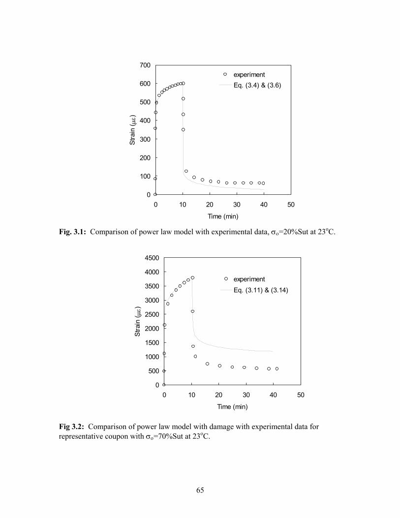
65

Fig. 3.1: Comparison of power law model with experimental data, σο=20%Sut at 23oC.

Fig 3.2: Comparison of power law model with damage with experimental data for representative coupon with σο=70%Sut at 23oC.

0

500

1000

1500

2000

2500

3000

3500

4000

4500

0 10 20 30 40 50

Time (min)

Stra

in ( µ

ε)

experimentEq. (3.11) & (3.14)

0

100

200

300

400

500

600

700

0 10 20 30 40 50

Time (min)

Stra

in ( µ

ε)

experimentEq. (3.4) & (3.6)

66

Fig 3.3: Comparison of preliminary shift factors obtained from creep testing with the WLF and Arrhenius relations, where the existence of a vertical shift factor is presumed.

Fig. 3.4: Comparison of vertical shift factor F(T) to experimental data.

0

0.5

1

1.5

2

2.5

3

3.5

4

290 300 310 320 330 340 350

Temperture (oK)

F(T)

-3.5

-3

-2.5

-2

-1.5

-1

-0.5

0

290 300 310 320 330 340 350

Temperature (oK)

log

(aT )

experimental

WLF(c1=6.885, c2=164.6)Arrhenius( Ea=64.2 kJ/mol)

Arrhenius (Ea=96.5 kJ/mol)

67

Fig. 3.5: Comparison of Eq. 3.24 and 3.25 with representative coupon with σo=37% Sut and T= 65oC.

Fig. 3.6: Master curve created using experimentally developed shift factors from DMA.

1.00E+09

1.00E+10

1E-07 0.0001 0.1 100 100000 1E+08 1E+11

Frequency (Hz)

E' (

Pa)

0

200

400

600

800

1000

1200

1400

1600

1800

2000

0 10 20 30 40

Time (min)

Stra

in ( µ

ε)

Eq.(3.24) & (3.25)experiment

68

Fig 3.7: Comparison of the shift factor found from DMA with the Arrhenius and WLF equations.

Fig. 3.8: Comparison of representative coupon master curve fit with preliminary horizontal and vertical shift factors used in Eq. (3.24) and a WLF horizontal shift determined by DMA.

0

0.2

0.4

0.6

0.8

1

1.2

1.4

0.1 10 1000 100000 10000000

t* (min)

D(t*

) (G

Pa-1

)

Eq. (3.24)WLF

1.00E-07

1.00E-06

1.00E-05

1.00E-04

1.00E-03

1.00E-02

1.00E-01

1.00E+00

20 30 40 50 60 70Temperature (oC)

aT

DMA

WLF (c1=20.5,c2=128.8)Arrhenius(Ea=325kJ/mol)

69

Fig. 3.9: Comparison of representative coupon with DMA time shift factor applied to power law with σο=43% Sut at 65oC.

Fig 3.10: Graphic reprensentation of the Prony Series model, taken from [24].

0

5000

10000

15000

20000

25000

0 10 20 30 40Time (min)

Stra

in ( µ

ε)

70

Fig. 3.11: Prony Series comparison with master curves for four coupons at σo=2.07 MPa. Inherent coupon to coupon variation is evident.

Fig. 3.12: Stress dependence of power law parameters Do and D1.

0

0.2

0.4

0.6

0.8

1

1.2

1.E-01 1.E+01 1.E+03 1.E+05 1.E+07

t* (min)

D(t)

(GPa

-1)

Prony Series

0

0.05

0.1

0.15

0.2

0.25

0.3

0.35

0 1 2 3 4 5 6Stress (MPa)

Do (

GPa

-1)

0

0.01

0.02

0.03

0.04

0.05

0.06

0.07

0.08

D1 (

GPa

-1m

in-n

)

Ο +∆ Coupons

71

Fig 3.13: Stress dependent parameters for non-linear Prony Series model.

Fig 3.14: Comparison of Prony Series model with representative coupon at 30% Sut at 23oC.

0

0.2

0.4

0.6

0.8

1

1.2

1.4

1 2 3 4 5

Stress (MPa)

go

0.3

0.5

0.7

0.9

1.1

1.3

1.5

1.7

1.9

2.1

a σ

-200

0

200

400

600

800

1000

1200

0 10 20 30 40 50

Time (min)

Stra

in ( µ

ε)

experimentEq. (3.31)

72

Fig 3.15: Comparison of Prony Series model with representative coupon with σο=43% Sut at 65oC.

Fig 3.16: Comparison of representative coupon with Prony Series model at σο=30% Sut at 45oC. Extensometer slippage is seen in recovery.

0

500

1000

1500

2000

2500

0 10 20 30 40

Time (min)

Stra

in ( µ

ε)


0

200

400

600

800

1000

1200

1400

1600

0 10 20 30 40 50

Time (min)

Stra

in ( µ

ε)


73

Fig 3.17: Comparison of representative coupon with Prony Series model with σο=30% Sut at 23oC. Recovery strain response phenomenon due to lab temperature fluctuation.

Fig 3.18: Threshold stress determination. ∆E=1-Ei/Ef where Ef is the final stiffness and Ei is the initial stiffness

-10%

0%

10%

20%

30%

40%

50%

0 20 40 60 80 100

% temperature dependent Sut

∆E

23 C45 C65 C

0

200

400

600

800

1000

1200

1400

1600

0 1000 2000 3000

Time (min)

Stra

in (m

e)


74

Fig 3.19: Convergence of Simpson’s rule for evaluation of Prony Series model incorporating damage.

Fig 3.20: Comparison of Prony Series model with representative coupon in creep at σο=50% Sut at 23oC.

0

0.2

0.4

0.6

0.8

1

1.2

1 10 100 1000 10000 100000

Number of iterations

Norm

aliz

ed s

train

0

500

1000

1500

2000

2500

0 5 10 15

Time (min)

Stra

in ( µ

ε)


75


Fig 3.22: Comparison of Prony Series model with representative coupon at σο=90% Sut at 23oC.

0

500

1000

1500

2000

2500

3000

3500

4000

4500

0 5 10 15

Time (min)

Stra

in ( µ

ε)


0

2000

4000

6000

8000

10000

12000

14000

0 5 10 15

Time (min)

Stra

in ( µ

ε)


76



0

500

1000

1500

2000

2500

3000

3500

0 5 10 15

Time (min)

Stra

in ( µ

ε)


0

2000

4000

6000

8000

10000

12000

0 5 10 15

Time (min)

Stra

in ( µ

ε)


77

REFERENCES [1] Rangaraj, Sudarshan V., Durability Assessment and Modeling of Wood-Thermoplastic Composites, Master’s Thesis, Washington State University, August 1999. [2] Rangaraj, Sudarshan V., and Smith, Lloyd V., The Non-linear Viscoelastic Response of a Wood-Thermoplastic Composite, Mechanics of Time-Dependent Materials, 3:125-139, 1999. [3] Lemaitre, Jean, and Chaboche, Jean-Loius, Mechanics of Solid Materials, Cambridge University Press, UK, 1990. [4] Smith, L.V., and Weitsman, Y.J., The visco-damage mechanical response of swirl mat composities, International Journal of Fracture, 92(3) 1999, 201-220. [5] Schwarzl, F. and Staverman, A.J., Time-Temperature Dependence of Linear Viscoelastic Behavior, Journal of Applied Physics, Vol 23 No 8, Aug 1952. [6] Nielsen, Lawrence F., and Landel, Robert F., Mechanical Properties of Polymers and Composites 2nd edition, Marcel Dekker, 1994. [7] Elahi, M., and Weitsman, Y.J., On the Mechanical response of P4 Chopped Glass/Urethane Resin Composite: Data and Model, Oak Ridge National Laboratory, ORNL –6955, October, 1999. [8] Crissman, J.M., Creep and Recovery Behavior of a Linear High Density Polyethylene and an Ethylene-Hexene Copolymer in the Region of Small Uniaxial Deformations, Polymer Engineering and Science, 26: n15, 1986 [9] Penn, Robert W.,Dynamic Mechanical Properties of Crystalline, Linear Polyethylene, Journal of Polymer Science: Part A-2, 4: 545-557 1966. [10] Fukui, Y., Sato, T., Ushirokawa, M., Asada, T, and Onogi, S., Rheo-Optical Studies of High Polymers. XVII. Time-Temperature Superposition of Time-Dependent Birefringence for High-Density Polyethylene, Journal of Polymer Science: Part A-2, Vol 8, 1195-1209, 1970. [11] Onogi, S, Sato, T., Asada, T, and Fukui, Y., Rheo-Optical Studies of Hight Polymers, XVIII. Significance of the Vertical Shift in the Time Temperature Superposition of RheoOptical and Viscoelastic Properties, Journal of Polymer Science: Part A-2 Vol 8, 1211-1255, 1970. [12] Morgan, C.J., Ward, I.M., The Temperature Dependence of Non-linear Creeep and Recovery in Oriented Polypropylene, Journal of the Mechanics and Physics of Solids, Vol. 19, pp165-178, 1971

78

[13] Brinson, L.C., Time-Temperature Response of Multi-phase Viscoelastic Solids through Numerical Analysis, PhD Thesis, California Institute of Technology, Feb 1990. [14] Williams, M.L., Landel, R.F., and Ferry, J.D., Journal of the American Chemical Society, 77, 3701, 1955. [15] Alkonis, John. J., and MacKnight, William J., Introduction to Polymer Viscoelasticity, 2nd edition, John Wiley and Sons, New York, 1983. [16] Callister, William D., Materials Science and Engineering: an Introduction, 3rd edition, John Wiley and Sons, 1994. [17] Van Krevelen, D.W., Properties of Polymers, Elsevier Scientific Publishing Company, Amsterdam, 1976. [18] Mark, James E., Physical Properties of Polymers Handbook, American Chemical Society, Washington D.C., 1993. [19] Sperling, L.H., Introduction to Physical Polymer Science, 2nd edition, John Wiley and Sons, 1992. [20] McCrum, N.G., Buckley, C.P., Bucknall, C.B., Principles of Polymer Engineering, Oxford University Press, New York, 1988. [21] Lai, J., and Bakker, A., Analysis of the non-linear creep of high-density polyethylene, Polymer, 36:1, 1995. [22] Schapery, R.A., ON the Characterization of Nonlinear Viscoelastic Materials, Polymer Engineering and Science, Vol. 9:4, July 1969. [23] Wood Handbook: Wood as an Engineering Material, Reprinted from the Forest Products Laboratory General Technical Report FPL-GTR-113 with the consent of the USDA Forest Service, Forest Products Society, 1999. [24] Gibson, Ronald F., Principles of Composite Material Mechanics, McGraw-Hill Inc., 1994.

79

CHAPTER FOUR

VISCOELASTIC FATIGUE RESPONSE OF WPC

4.1 Introduction

Much of the study on fatigue undertaken for viscoelastic materials has been in the

areas of predicting fatigue life and crack growth. Further, study of the effects of fatigue

on the viscoelastic properties E’, E” and tan δ has also been undertaken. However, little

has been done with predicting the strain response of a viscoelastic material in cyclic

loading. After the successful application of the Prony Series viscoelastic model to a step

stress input at various temperatures, the competence of the model to predict the strain

response of the WPC when subjected to a cyclic loading scenario was investigated.

Previous work in the viscoelastic modeling of fatigue loading conducted by Elahi and

Weitsman [1] utilized a cyclic ramp loading function on a glass/urethane composite.

Temperature dependence was not incorporated into their model. Some comparison

between creep behavior and fatigue behavior of HDPE to a cyclic displacement has also

been studied by Scavuzzo [2] and He [3] at room temperature, but a model was not

developed to describe the behavior.

The present work will develop a model to describe the viscoelastic behavior of the

WPC in fatigue loading. This will be accomplished by applying a sinusoidal stress

function to the creep models developed in Chapter Three. The temperature dependence,

stress dependence, and damage developed for creep loading will also be utilized in the

viscoelastic fatigue model presented herein.

80

4.2 Power Law Model

4.2.1 Development of power law fatigue model

The power law established by Rangaraj and Smith [4] was utilized to describe the

viscoelastic fatigue response. This model, while found not to adhere to the strict

application of the TTSP provided a convenient expression for cyclic response. The

application of a cyclic load to the viscoelastic model can be modeled by replacing the

step stress function in the convolution integral Eq. (3.1) with the an equation for cyclic

stress

( ) )()sin()( tHftt amf σσσ += (4.1)

where f is the frequency of the oscillation in minutes, σm is the mean cyclic stress, and σa

is the stress amplitude. Again, H(t) is the Heaviside step function which controls the

onset of the cyclic stress. Evaluating this stress function with the power law compliance

in the convolution integral produces

[ ] [ ] ττστσε dfftDDtDt a

t nom )cos()()()(

0 1 ⋅−⋅++⋅= ∫ (4.2)

which does not have a closed form solution as n is not an integer. Simpson’s rule was

chosen to numerically integrate this equation. In order to efficiently calculate the strain

response due to fatigue loading, a Fortran program was written to perform this integration

and record the peak strain response of the first cycle of every minute. This program is

attached in Appendix 1. The frequency f in cycles per minute was calculated as

2π(γ)60 where γ is the frequency in Hertz. The time at which the first peak strain

occurred immediately after each minute was calculated as (4(60)(γ))-1min-1.

A convergence study was completed to determine the number of iterations

required for convergence at 100 minutes, 500 minutes and 10,000 minutes. It was found

81

that the strain response converged at a variable number of iterations equal to 5,000t,

where t is the time at which the peak strain is being evaluated. Also, the value of the

strain response predicted by the Fortran model at 5,000t was within 2% of the response

predicted at twice the number of iterations at each of the times studied, as can be seen in

Fig. 4.1.

4.2.2 Experimental verification

In order to minimize the inherent scatter observed between coupons, prior to

fatigue testing, a 10-minute creep and recovery test to 30% Sut at 23oC was conducted.

This allowed the values for the parameters Do and D1 to be determined for each coupon,

removing some of the variability which would have resulted had average values of Do

and D1 been used. A comparison of the power law model to the creep recovery for a

representative coupon is shown in Fig. 4.2. The parameters from this comparison were

found to be Do= .273 Gpa-1 (1.88 Msi-1), D1=.032 Gpa-1min-n ( 0.22 Msi-1/min-n). As was

discussed in Chapter Two, a frequency of 0.5Hz was used for fatigue testing due to the

reduced slippage of the extensometer and the absence of detectable temperature effects.

Specimens were loaded in fatigue at 23oC with σmax=30%Sut and R=0.1 as described in

Chapter Two. A comparison of the peak cyclic strain from Eq. (4.2) with a representative

coupon is shown in Fig 4.3. Fig 4.4 compares the strain response of the model with that

same coupon for times greater than 100 minutes. This indicates that while the first five

minutes appear to have about the same time dependence, and strain response, the time

dependence of the viscoelastic model is greater than that observed experimentally. By

viewing the behavior at times nearing 1000 minutes, it is easy to see that the WPC

initially has a rapid strain response initially, but soon the strain response nearly flattens

82

out. The viscoelastic model developed with the power law, conversely, continues to

climb as time increases, and does not appear to nearly flatten out, even after 1000

minutes.

4.2.3 Time-temperature superposition of power law model

The preliminary vertical and horizontal temperature shift factors utilized in Eq.

(3.24) were applied to the model to predict temperature dependence of the fatigue

response as

( )[ ] ( )[ ] ττστσε dfftDTFDTa

tDTFDt aTa

tn

omT

oT cos)()

)(~()()( )(~

0 11 ⋅−⋅++⋅

+= ∫ (4.3)

where F(T) is the instantaneous shift factor and )(~ TaT is the preliminary time dependent

shift factor. Coupons were loaded to 30% Sut at 45oC and 65oC. The Fortran model

predicted the strain response at a temperature by evaluating the model at the applied

stress levels at shifted time. In order to compare the experimental results and the power

law model on the same time scale, the time data given by the model was multiplied by the

time shift factor for the temperature. A representative coupon at 65oC with R=0.1 is

shown in Fig. 4.5. The comparison shows that time dependence is over-predicted by the

model. Likewise, the magnitude of the predicted behavior is approximately twice that of

the experimental response.

4.2.4 Power law viscoelastic behavior of other polymeric materials

Due to the inability of the power law viscoelastic model to predict the behavior of

the WPC in fatigue at any temperature, questions were raised as to whether this was a

phenemonon of the fatigue responses of HDPE, or whether this was a shortcoming of the

viscoelastic fatigue model. Specimens of virgin HDPE, a polypropylene (PP) based

83

WPC, and a poly-vinyl chloride (PVC) based WPC were acquired. Several coupons of

the PP WPC and virgin HDPE were dogboned to the same dimensions as the HDPE

based WPC studied in this work for quasi-static testing to determine strength and elastic

modulus. The PVC was not dogboned, due to dimensional limitations of the source

material. This resulted in a lower measured Sut as failure in quasi-static testing occurred

at the stress concentration at the grips. These coupons were also 7.6 mm thick instead of

12.7mm, as were the other coupons. Table 4.1 lists the results of this testing. Values for

the HDPE WPC studied in this work are also listed for comparison.

Table 4.1 Comparison of strength and elastic modulus for viscoelastic materials tested. Material Strength

(MPa) Elastic

Modulus (GPa)

Do (GPa-1)

D1 (GPa-1)

n

Virgin HDPE 19.8 1020 .783 .333 .3

PP-WPC 11.6 4040 .174 .015 .3

PVC-WPC 22.5 6840 .13 .013 .19

HDPE WPC 10.7 3800 ~.27 ~.033 .39

As observed in Table 4.1, the primary benefit of the wood component is to

increase stiffness and reduce time dependence. Straight coupons were cut to the same

dimensions as those described in Chapter Two for the WPC used in this work, excluding

the thickness of the PVC specimens. These coupons were loaded in creep to

approximately 30% of their ultimate strength at 23oC, as found by the quasi-static

loading, for 10 minutes and allowed to recover. The values of Do, D1, and n were chosen

to obtain a best fit with the power law for each coupon. These coupons were then loaded

in fatigue to approximately 30% of the experimentally determined ultimate strength at

84

23oC for between 90 and 600 minutes. The viscoelastic fatigue model was applied using

the parameters obtained from Table 4.1 for each material.

Fig. 4.6-4.11 show a comparison for a representative coupon of each material

compared to the power law model for creep and recovery then the corresponding fatigue

experimental and predicted response. In Fig. 4.7, the viscoelastic fatigue model

developed for the virgin HDPE coupon continues to indicate a greater time dependence

than is observed in the experimental fatigue response, in the same way as it did for the

HDPE WPC under investigation. In comparison, while the initial offset doesn’t quite

match, the time dependence of the strain response of the PP-WPC and PVC-WPC

appears to closely match the experimental data as can be seen in Fig. 4.9 and Fig 4.11.

This indicates further that the power law viscoelastic model does not describe well the

behavior of HDPE, as was seen in the previous chapter.

In their study of the continuous and dynamic stress relaxation of HDPE,

Scavuzzo[2] and Fe[3] observed different time dependent relaxations. In their testing,

HDPE coupons were displaced a specified amount. Some were allowed to relax under

monotonic displacement, while others were given a cyclic displacement oscillating

around the constant displacement applied to the monotonic coupons. A summary of their

results is shown in Fig 4.12. Note that rapid relaxation is observed initially in fatigue

loading, which then levels out as time increases. In monotonic displacement, however, a

slower initial relaxation with a greater time dependence is observed. This is similar to the

results shown in Fig 4.3, and 4.4 where the coupons exhibit an immediate strain response,

then the strain response tends to flatten out.

85

4.3 Prony Series Model

4.3.1 Development of the Prony Series fatigue model

In spite of the apparent contradictions between the creep and fatigue response of

the WPC observed with the power law, the Prony Series compliance was applied to

fluctuating stress. The development of the Prony Series fatigue model was very similar

to the power law development. Eq. (4.2) was applied to the convolution integral with the

Prony Series compliance. This resulted in a time, stress, and temperature dependent

strain as

( )[ ] ττσσσεσ

ττ

τ dffeDDgeDDgTt a

Taat

n

t

nooon

Tat

noo

T

nTn sin)1()1(),,()(

0

5

1

5

1

)( ∫ ∑∑

−++

−+=

=

+−

=

−

(4.4)

where the integrand, denoted G(t,τ) must be approximated with Simpson’s rule, as was

described above. This can be represented as

∑∫=

+

−

+

−

=−N

i NittG

NittG

NittG

NtdtG

1

,5.,41,6

)( ττ (4.5)

where N is the number of iterations. The same number of iterations per minute (5,000t)

used for the power law model was found to be sufficient in evaluating the prony series, as

can be seen in the convergence study in Fig 4.13. For times of 100 and 1000 minutes of

fatigue, the strain response at 5,000t iterations was found to be within 2% of the response

found with a number of iterations an order of magnitude higher. This study was

performed with σm=1.35MPa and σa=1.10MPa. A copy of the prony series viscoelastic

fatigue Fortran model is attached in Appendix 2. The stress dependence observed in the

creep modeling of the WPC was also utilized in modeling the fatigue behavior. The

86

stress dependence was calculated at the peak stress, σm+σa, where the strain response was

evaluated.

4.3.2: Experimental verification of Prony Series model

As can be seen from Fig. 4.14 and Fig 4.15, the time dependence predicted by the

Prony Series model is very similar to that exhibited by the material. The difference in the

instantaneous magnitude of the model and the experiment is due to coupon stiffness

variation. Fig. 4.15 shows a comparison of the power law model, the Prony Series model,

and the experimental data utilizing the same coupon as shown in Fig. 4.3 and Fig. 4.4.

While also indicating the inherent variability between coupons, it also shows that the

Prony Series model predicts the time dependence of the material in fatigue quite well at

23oC.

4.3.3 Time-temperature superposition in Prony Series model

The temperature shift factor was accounted for in the same way as was used for

the power law. The number of iterations was increased to 15,000t. The time data from

the Prony Series model was multiplied by the shifted time to enable comparison with

experimental data. As can be seen from Fig. 4.16, predicted strain response was very

similar in magnitude to the experimental strain at σmax=30% at 45oC. The time

dependence was greater than experimentally observed. The magnitude of the

experimental strain response was seen to vary between coupons. While the predicted

viscoelastic behavior is much closer to experimental behavior than was observed for the

power law model, it appears that the Prony Series viscoelastic fatigue model does not

describe the mechanisms involved in fatigue of the WPC at elevated temperatures.

87

4.4 Damage Applied to Models

4.4.1 Power law fatigue model with damage

In order to account for fatigue loading where specimens were subjected to stresses

above their threshold stress, a fatigue model for damage was developed. The damage

function utilized for the creep models was also utilized for fatigue. For the power law

model, damage was described as

>−<++= dfm

f ctst σσσω )(1),( (4.6)

where σf is given by Eq. (4.1). The function inside the McCauly brackets may be

represented as

))(())(( dfdfdf tHt σσσσσσ −−>=−< (4.7)

where H is the Heaviside step function. Subsequent differentiation of the effective stress

)(),()()( tHttt ffe ⋅⋅= σωσσ (4.8)

which is evaluated together with the time dependent compliance in the convolution

integral produces the viscoelastic response of the WPC to fatigue as

( )( )τ

σστστσ

σστστσωτστσσσε d

tHffcst

tmctfftDtDt

t

dfam

f

dfm

ffadmm ∫

−+

+−+−+−=

−

0

1

))(()cos()(

)()(),()cos()()()(

(4.9)

where the integrand must be numerically integrated and where D(t) is given by Eq. (3.3)

in the previous chapter and the damage parameters are the same as given in Chapter

Three. Simpson’s rule was chosen to evaluate the integral. Many more integrations per

time step were required for adequate modeling of the fatigue response. This can be seen

88

from Fig. 4.17 where 15,000t iterations were required for convergence. This is due to the

sudden vertical jump in strain response that occurs as the applied stress passes through

the threshold stress and discontinuities result in the model as strain suddenly increases

with the application of damage. The program used to evaluate Eq. (4.9) (included in

Appendix 3) was verified by comparison of its results with the linear fatigue model. A

comparison of the model for a representative coupon at R=0.1, σmax=70% Sut at 23oC is

shown in Fig. 4.18. The power law does not match the experimentally observed time

dependence when damage is present.

4.4.2 Prony Series fatigue model with damage

To account for damage in the non-linear Prony Series, the same damage model

utilized for the power law model, Eq. (4.6), was used. This was developed in the same

way as the power law damage model, where the Prony Series was used for the

compliance in Eq. (4.9). As found previously for the Prony Series, s=0, and

c=.160GPa-1min-m. The program used to evaluate Eq. (4.9) (included in Appendix 4) was

verified by comparison of its results with the linear fatigue model. Above 43% Sut, the

non-linear terms were evaluated at the threshold stress as was determined for creep

loading. A comparison with experimental strain response and the power law model is

shown in Fig. 4.18. The Prony Series model does not model the behavior of the WPC

above the threshold stress well in either time dependence or magnitude. Damage is

overpredicted in this model.

4.4.3 Fatigue damage discussion

While the damage model utilized worked well in creep loading, it did not

characterize the damage occuring in fatigue. The continuum damage function, Eq. (4.6),

89

presumes that there is an instantaneous (s) and time dependent (c) portion of damage that

increases with time above the threshold stress. No instantaneous damage was found

during creep loading with the Prony Series model. From Fig. 4.18, it appears that the

time dependent damage is too great, as this is the only damage affecting the model. As

damage is applied in the model, it accrues as long as the stress is above the threshold

stress. This apparently is not what occurs in the actual fatigue of the WPC at hand.

Likely, after the initial damage accumulation during the first few cycles, material damage

only occurs at the peaks of the stress cycle, imparting a much smaller amount of damage

per cycle than is predicted by the current damage model. It would appear from the

experimental data, that crazing occurs or microcracks form during the initial few cycles

of the fatigue loading. These cracks are then prevented from propagating by the wood

particles or by blunting and softening of the crack tips due to hysteretic heating.

However, X-ray computed Tomography (CT) performed on a sample of the WPC

loaded to 70% Sut in fatigue did not discern the formation of microcracks on the

mesoscopic scale. The spatial resolution of the CT scanner was 0.27mm, which may be

greater than the size of the microcracks if present. Damage, presenting itself through a

change in density of the material, however, was observed to occur though CT analysis in

the specimens previously loaded in creep and fatigue although the nature of the damage

was not evident from the analysis. Temperature dependent damage was also observed in

CT scanning.[5] While not indicating how the damage model was inadequate for fatigue

loading, CT analysis does indicate the presence of damage and appeared to show

quantitative differences in damage between creep and fatigue loading. The damage

90

function used to describe the creep behavior is insufficient for modeling the behavior of

the WPC in fatigue loading.

A comparison of the percent reduction in elastic modulus is given in Fig. 4.19 for

fatigue loading. This indicates the relative damage occurring between coupons loaded in

fatigue for 100 minutes with σmax=30% and 70% of the temperature dependent Sut. A

qualitative comparison with creep data can be made using Fig. 3.18, which indicates the

reduction in elastic modulus after a 10 minute creep test as a function of applied load.

Note that at 70% Sut, the change in modulus after 100 minutes of fatigue is slightly lower

than was observed after 10 minutes of creep. This supports the peak strain comparisons,

which also indicate slower damage growth in fatigue. Interestingly, temperature induced

damage below the threshold stress observed for creep in Fig. 3.18 are not as apparent in

Fig. 4.19.

Due to the inability of the Prony Series model to describe the strain response of

the WPC at temperatures above 23oC in creep above the threshold stress, modeling of the

fatigue response above the threshold stress at temperatures above 23oC was not

attempted.

4.4 Summary

The power law models appears to be insufficient for modeling the viscoelastic

response in fatigue loading for the WPC at hand at room temperature at room

temperature, and at the other temperatures tested. However, it does appear to describe

the viscoelastic fatigue response of other polymeric materials at room temperature,

indicating that the power law may be a better fit for those other materials than it is for the

WPC under investigation. The viscoelastic response predicted by the Prony Series

91

model, while slightly above the experimental response, showed the same time

dependence as the experimental response at room temperature. At elevated temperatures,

it appeared that the Prony Series model was no longer describing the behavior of the

material.

Neither the Prony Series nor the power law model were sufficient to describe the

behavior of the WPC when the fatigue cycle included some of the region above the

threshold strength. While the damage model utilized in creep worked well in creep

loading, it does not characterize the damage occurring in fatigue loading.

92

Fig 4.1: Convergence study for Fortran fatigue model using Simpson’s rule.

Fig 4.2 Comparison of power law model to 10 minute creep/recovery data at 30%Sut, 23oC.

0

0.2

0.4

0.6

0.8

1

1.2

1.E+03 1.E+04 1.E+05 1.E+06 1.E+07 1.E+08

Iterations

Norm

aliz

ed s

train

100 min500 min10,000 min

0

200

400

600

800

1000

1200

0 10 20 30 40 50

Time (min)

Stra

in ( µ

ε)

modelexperiment

93

Fig 4.3: Comparison of peak cyclic strains of fatigue model using coupon dependent parameters with experimental data, R=0.1, σmax=30% Sut at 23oC.

Fig 4.4: Same coupon as Fig. 4.3 showing 800 minutes of data for comparison.

0

200

400

600

800

1000

1200

1400

1600

1800

0 200 400 600 800Time (min)

Stra

in ( µ

ε)

experimentmodel

0

200

400

600

800

1000

1200

1400

0 20 40 60 80 100

Time (min)

Stra

in ( µ

ε)

experimentmodel

94

Fig 4.5: Comparison of viscoelastic power law model and representative coupon at 65oC and σmax=30%Sut with R=0.1. Power law model time is multiplied by aT(T) according to the time shift factor of Eq. (3.24), for comparison with experimental data.

Fig 4.6: Comparison between power law model for HDPE and representative coupon. Do=.783 Gpa-1 (5.4 Msi-1) D1=.333 Gpa-1min-n (2.3 Msi-1min-n) n=0.30, σo=3.17MPa.

0

1000

2000

3000

4000

5000

6000

7000

0 10 20 30 40 50

Time (min)

Stra

in ( µ

ε)

modelexperiment

0

200

400

600

800

1000

1200

1400

1600

1800

2000

0 50 100 150

Time (min)

Stra

in ( µ

ε)

experimentpower law

95

Fig 4.7: Comparison of HDPE power law fatigue model and representative coupon, σmax=4.1 MPa with R=0.1, f=0.5 Hz.

Fig 4.8: Comparison between power law model for PP WPC and representative coupon. Do=.174 Gpa-1 (1.205 Msi-1) D1=.015 Gpa-1min-n (.10 Msi-1min-n) n=0.30, σo=3.17MPa.

0

1000

2000

3000

4000

5000

6000

7000

8000

0 100 200 300

Time (min)

Stra

in ( µ

ε)

experimentmodel

-100

0

100

200

300

400

500

600

700

800

0 10 20 30 40 50

Time (min)

Stra

in( µ

ε)

modelexperiment

96

Fig 4.9: Comparison of PP WPC power law fatigue model and representative coupon, σmax=3.17MPa with R=0.1, f=0.5 Hz.

Fig 4.10: Comparison between power law model for PVC WPC and representative coupon. Do=.13 Gpa-1 (0.9Msi-1) D1=.013 Gpa-1min-n (.09 Msi-1min-n) n=0.19, σo=9.72MPa.

0

100

200

300

400

500

600

700

800

900

0 100 200 300 400 500 600

Time (min)

Stra

in (m

e)

experimentmodel

0

200

400

600

800

1000

1200

1400

1600

0 10 20 30 40 50

Time (min)

Stra

in(m

e)

modelexperiment

97

Fig 4.11: Comparison of PVC WPC power law fatigue model and representative coupon, σmax=9.72MPa with R=0.1, f=0.5 Hz.

0

200

400

600

800

1000

1200

1400

1600

1800

0 20 40 60 80 100Time (min)

Stra

in ( µ

ε)

experimentmodel

98

Fig 4.12: Dynamic relaxation compared to relaxation from monatonic displacement. Taken from thesis of Fang He [3].

99

Fig 4.13: Convergence study for Prony Series fatigue model.

Fig 4.14: Comparison of Prony Series model with experimental data at 23oC and σmax=30%Sut with R=.1.

0

200

400

600

800

1000

1200

1400

0 200 400

Time (min)

Stra

in (

)

experimentmodel

0

0.2

0.4

0.6

0.8

1

1.2

1.E+04 1.E+05 1.E+06 1.E+07 1.E+08

Number of iterations

Norm

aliz

ed s

train

100 min1000 min

100

Fig 4.15: Comparison of Prony Series model with power law and experimental data for the coupon shown in Fig 4.3 and 4.4.

Fig. 4.16: Comparison of representative coupon and Prony Series model at 45oC and σmax=30%Sut with R=0.1. Shifted time from Fortran model is multiplied by aT to compare with real time measured experimentally.

0

200

400

600

800

1000

1200

1400

1600

1800

0 200 400 600

Time (min)

Stra

in ( µ

ε)

Power Law

experiment

Prony Series

0

200

400

600

800

1000

1200

1400

0 50 100 150 200

Time (min)

Stra

in ( µ

ε)

experiment

prony series

101

Fig 4.17: Convergence of the power law damage model at 100 minutes. 15,000t iterations required.

Fig 4.18: Comparison of power law model an Prony Series model to representative coupon at 23oC and σmax=70%Sut with R=0.1.

0

0.2

0.4

0.6

0.8

1

1.2

1.E+04 1.E+05 1.E+06 1.E+07 1.E+08

Number of Iterations

Norm

aliz

ed s

train

0

1000

2000

3000

4000

5000

6000

0 20 40 60 80 100

Time (min)

Stra

in ( µ

ε)

experiment

power law

prony series

102

Fig. 4.19: Percent reduction in elastic modulus ∆E=1-Ei/Ef in fatigue loading where Ef is the final stiffness and Ei is the initial stiffness.

-4.00%

-2.00%

0.00%

2.00%

4.00%

6.00%

8.00%

10.00%

12.00%

0% 20% 40% 60% 80%

% temperature dependent Sut

∆E

23 C45 C65 C

103

REFERENCES [1] Elahi, M., and Weitsman, Y.J., On the Mechanical response of P4 Chopped Glass/Urethane Resin Composite: Data and Model, Oak Ridge National Laboratory, ORNL –6955, October, 1999. [2] Scavuzzo, Rudolph J., Oscillating Stress on Viscoelastic Behavior of Thermoplastic Polymers, Journal of Pressure Vessel Technology, Vol. 122, August 2000. [3] He, Fang, Fatigue and Stress Relaxation Behavior of High-Density Polyethylene, Master’s Thesis, University of Akron, December, 1997. [4] Rangaraj, Sudarshan V., and Smith, Lloyd V., The Non-linear Viscoelastic Response of a Wood-Thermoplastic Composite, Mechanics of Time-Dependent Materials, 3:125-139, 1999. [5] Shi, Q., and Bathias, C., Analytical results from X-ray computed Tomography on wood plastic composite, ITMA/CNAM, Paris, March 2001.

104

CHAPTER FIVE

CONCLUSIONS AND RECOMMENDATIONS

5.1 Conclusions

The power law and Prony Series viscoelastic models were evaluated in their

ability to describe the time dependent behavior of the wood-plastic composite in creep

and fatigue loading. The WPC was found to be thermo-rheologically simple according

tests conducted with DMA. The horizontal shift factor was described satisfactorily by the

WLF equation. While the power law was adequate for describing the behavior at short

times and an equation with preliminary shift factors was readily obtainable for describing

the temperature dependence of the WPC for short times, it was not found to describe well

the behavior of the WPC when the TTSP was applied using the DMA shift factor. A

Prony Series model was developed, which, while more complex, was able to describe the

creep response for up to 107 minutes (in shifted time) based on the TTSP. Good

correlation was obtained between experimental data and the Prony Series model at 23oC,

45oC, and 65oC. The threshold stress was found to scale with the temperature dependent

ultimate strength. A continuum damage model was developed to describe the strain

response for the WPC at 23oC but overpredicted the strain response at elevated

temperatures above the threshold stress indicating that the magnitude of damage was

temperature dependent.

Application of the creep viscoelastic model to predict the peak cyclic strain during

fatigue loading was undertaken. Good correlation between the Prony Series and the

experimental data at 23oC was obtained. Temperature was found to affect the cyclic

strain response for the WPC, such that the model did not satisfactorily predict the strain

105

response. Likewise, above the threshold stress, the damage model did not predict the

strain response, indicating that the time dependence damage as accounted for by the creep

model does not match the behavior of the WPC in cyclic loading.

The viscoelastic behavior of the WPC is not described by a simple model. Rather,

it must be described by a non-linear Prony Series model that allows for modeling of the

several time dependent viscoelastic behaviors of the material. Additionally, the material

behaves non-linearly, requiring stress dependent terms. A threshold stress is also

observed, requiring a damage model to represent behavior above the threshold stress.

The damage was found to be dependent on temperature, and on the loading function.

5.2 Recommendations:

Further creep tests performed for longer durations at the three temperatures tested

would increase the time period that could be described by the Prony Series model at

various temperatures. Further, if creep tests were performed at more frequent

temperature intervals, perhaps every 5oC, superposition of the creep curves could be

conducted, producing a more complete compliance master curve without gaps. This

could be used to develop a master curve and time shift factor aT(T) without using DMA.

This would further the predictive ability of the model over a wide range of elevated

temperatures below the melting point.

Further investigation of the viscoelastic behavior at temperatures below 23oC

would provide a complete understanding of the temperature dependent behavior of this

material.

Use of a technique such as computed Tomography scanning of the WPC to

compare the structure before and after creep, cyclic, and temperature loading at a greater

106

variety of loading scenarios would provide information on the changing nature of the

damage mechanism with temperature and loading. This may provide directions as to the

type of damage model required to predict the behavior of the WPC under cyclic loading,

however, the inclusion of these findings may further convolute the already complex

model.

APPENDIX ONE

Power law fatigue model below threshold strength

108

implicit double precision (a-h,o-z)

integer i,j,k,N c c-----define functions c FT=stiffness shift factor c aT=time shift factor c f(x,y)=function being integrated c g(z) is function before integral g(z)=d0*FT+done*(z)**dn f(x,y)=(d0*FT+done*(((x-y))**dn))*(w)*sigamp*cos(w*y) c k=50 c c define realn as real number for use in equation c realn=N c c-----defining constants c pi=3.14159265358979323846 sigamp=207 sigmean=253 c temp in kelvin temp=296 tref=296. d0=1.6 FT=.0441*temp-12.05 done=.22 dn=.39 freq=.5 offset1=1./(4.*60.*freq) w=2.*pi*60.*freq aT=10.**((-6.885*(temp-tref))/(164.6+temp-tref)) c c write format for output file c iin=10 iout=11 open (unit=11,status='unknown',file='23C30%pwl',form='formatted') c c evaluate integral using simpson's rule c do 100 j=0,k realj=(1.+16.*j)*offset1 Sn=0. sum=g(realj/aT)*sigmean

109

N=j*5000 realn=N c do 200 i=2,N reali=i c realn=N c continuing with simpson's rule c c sum=sum+(realj/(6.*realn))*(f(realj,realj*(reali-1.)/realn)+ c . 4.*f(realj,realj*(reali-.5)/realn)+f(realj,realj*reali/realn)) c c c---- loop for calculating max strain for first cycle of each minute c c sum1=f(realj,realj*(reali-1.)/realn) c sum2=f(realj,realj*(reali-.5)/realn) c sum3=f(realj,realj*(reali)/realn) Sn=(realj/(6.*realn))*(sum1+4.*sum2+sum3)+Sn c 200 end do Sn=Sn+sum c c create output file c write(11,1000) realj/aT,Sn c 1000 format(e25.14,e25.14) 100 end do end

APPENDIX TWO

Prony series fatigue model below threshold stress

111

implicit double precision (a-h,o-z) integer i,j,k,N c c-----define functions c aT=time shift factor c f(x,y)=function being integrated c g(z) is function before integral h(u)=sigmean+sigamp*sin(w*u) diff(t)=(h(t)-thresh)*step g(z)=d0*b+d1*(1-exp(-z/tau1))+ .d2*(1-exp(-z/tau2))+d3*(1-exp(-z/tau3)) .+d4*(1-exp(-z/tau4))+d5*(1-exp(-z/tau5)) c f(x,y)=g(x-y)*w*sigamp*cos(w*y)*(1+(s+dc*y**dm)*diff(y)) .+g(x-y)*h(y)*(dm*dc*y**(dm-1)*diff(y)+ .(s+dc*y**dm)*w*sigamp*cos(w*y)*step) c k=100 c c-----defining constants c pi=3.14159265358979323846 sigamp=490. sigmean=600. c temp in kelvin temp=296. tref=296. d0=1.94 d1=.65 tau1=20. d2=.9 tau2=1000 d3=.8 tau3=12000 d4=1.126 tau4=148641 d5=1.8748 tau5=3000000 freq=.5 offset1=1./(4.*60.*freq) w=2.*pi*60.*freq dm=0.15 s=.00 dc=.0011

112

c threshold stress of .43% Sut thresh=670. aT=10.**((-20.534*(temp-tref))/(128.78+temp-tref)) c if (sigamp+sigmean.gt.thresh) then b=.000563*(thresh)+.8225 c=-.00171*(thresh)+1.8555 else b=.000563*(sigamp+sigmean)+.8225 c=-.00171*(sigamp+sigmean)+1.8555 end if c c write format for output file c iin=10 iout=11 open (unit=11,status='unknown',file='23C70%62',form='formatted') c c evaluate integral using simpson's rule c do 100 j=0,k realj=(j+offset1) Sn=0. sum=g(realj/(c*aT))*sigmean N=j*50000 realn=N c do 200 i=2,N reali=i c realn=N c continuing with simpson's rule c c sum=sum+(realj/(6.*realn))*(f(realj,realj*(reali-1.)/realn)+ c . 4.*f(realj,realj*(reali-.5)/realn)+f(realj,realj*reali/realn)) c c c---- loop for calculating max strain for first cycle of each minute c if (h(realj*(reali-1.)/realn) .le. thresh) then step=0. else step=1. end if sum1=f(realj,realj*(reali-1.)/realn) c if (h(realj*(reali-.5)/realn) .le. thresh) then

113

step=0. else step=1. end if sum2=f(realj,realj*(reali-.5)/realn) c if (h(realj*(reali)/realn) .le. thresh) then step=0. else step=1. end if sum3=f(realj,realj*(reali)/realn) Sn=(realj/(6.*realn))*(sum1+4.*sum2+sum3)+Sn c c c 200 end do Sn=Sn+sum c c create output file c write(11,1000) realj/(c*aT),Sn c 1000 format(e25.14,e25.14) 100 end do end

APPENDIX THREE

Power law Fortran fatigue model with damage

115

implicit double precision (a-h,o-z)

integer i,j,k,N c c-----define functions c aT=time shift factor c f(x,y)=function being integrated c g(z) is function before integral h(u)=sigmean+sigamp*sin(w*u) diff(t)=(h(t)-thresh)*step g(z)=d0*b+d1*(1-exp(-z/tau1))+ .d2*(1-exp(-z/tau2))+d3*(1-exp(-z/tau3)) .+d4*(1-exp(-z/tau4))+d5*(1-exp(-z/tau5)) c f(x,y)=g(x-y)*w*sigamp*cos(w*y)*(1+(s+dc*y**dm)*diff(y)) .+g(x-y)*h(y)*(dm*dc*y**(dm-1)*diff(y)+ .(s+dc*y**dm)*w*sigamp*cos(w*y)*step) c k=100 c c-----defining constants c pi=3.14159265358979323846 sigamp=490. sigmean=600. c temp in kelvin temp=296. tref=296. d0=1.94 d1=.65 tau1=20. d2=.9 tau2=1000 d3=.8 tau3=12000 d4=1.126 tau4=148641 d5=1.8748 tau5=3000000 freq=.5 offset1=1./(4.*60.*freq) w=2.*pi*60.*freq dm=0.15 s=.00 dc=.0011 c threshold stress of .43% Sut

116

thresh=670. aT=10.**((-20.534*(temp-tref))/(128.78+temp-tref)) c if (sigamp+sigmean.gt.thresh) then b=.000563*(thresh)+.8225 c=-.00171*(thresh)+1.8555 else b=.000563*(sigamp+sigmean)+.8225 c=-.00171*(sigamp+sigmean)+1.8555 end if c c write format for output file c iin=10 iout=11 open (unit=11,status='unknown',file='23C70%62',form='formatted') c c evaluate integral using simpson's rule c do 100 j=0,k realj=(j+offset1) Sn=0. sum=g(realj/(c*aT))*sigmean N=j*15000 realn=N c do 200 i=2,N reali=i c realn=N c continuing with simpson's rule c c sum=sum+(realj/(6.*realn))*(f(realj,realj*(reali-1.)/realn)+ c . 4.*f(realj,realj*(reali-.5)/realn)+f(realj,realj*reali/realn)) c c c---- loop for calculating max strain for first cycle of each minute c if (h(realj*(reali-1.)/realn) .le. thresh) then step=0. else step=1. end if sum1=f(realj,realj*(reali-1.)/realn) c if (h(realj*(reali-.5)/realn) .le. thresh) then step=0.

117

else step=1. end if sum2=f(realj,realj*(reali-.5)/realn) c if (h(realj*(reali)/realn) .le. thresh) then step=0. else step=1. end if sum3=f(realj,realj*(reali)/realn) Sn=(realj/(6.*realn))*(sum1+4.*sum2+sum3)+Sn c c c 200 end do Sn=Sn+sum c c create output file c write(11,1000) realj/(c*aT),Sn c 1000 format(e25.14,e25.14) 100 end do end

APPENDIX FOUR

Prony series Fortran fatigue model with damage

119

implicit double precision (a-h,o-z) integer i,j,k,N c c-----define functions c aT=time shift factor c f(x,y)=function being integrated c g(z) is function before integral h(u)=sigmean+sigamp*sin(w*u) diff(t)=(h(t)-thresh)*step g(z)=d0*b+d1*(1-exp(-z/tau1))+ .d2*(1-exp(-z/tau2))+d3*(1-exp(-z/tau3)) .+d4*(1-exp(-z/tau4))+d5*(1-exp(-z/tau5)) c f(x,y)=g(x-y)*w*sigamp*cos(w*y)*(1+(s+dc*y**dm)*diff(y)) .+g(x-y)*h(y)*(dm*dc*y**(dm-1)*diff(y)+ .(s+dc*y**dm)*w*sigamp*cos(w*y)*step) c k=100 c c-----defining constants c pi=3.14159265358979323846 sigamp=490. sigmean=600. c temp in kelvin temp=296. tref=296. d0=1.94 d1=.65 tau1=20. d2=.9 tau2=1000 d3=.8 tau3=12000 d4=1.126 tau4=148641 d5=1.8748 tau5=3000000 freq=.5 offset1=1./(4.*60.*freq) w=2.*pi*60.*freq dm=0.15 s=.00 dc=.0011 c threshold stress of .43% Sut thresh=670.

120

aT=10.**((-20.534*(temp-tref))/(128.78+temp-tref)) c if (sigamp+sigmean.gt.thresh) then b=.000563*(thresh)+.8225 c=-.00171*(thresh)+1.8555 else b=.000563*(sigamp+sigmean)+.8225 c=-.00171*(sigamp+sigmean)+1.8555 end if c c write format for output file c iin=10 iout=11 open (unit=11,status='unknown',file='23C70%62',form='formatted') c c evaluate integral using simpson's rule c do 100 j=0,k realj=(j+offset1) Sn=0. sum=g(realj/(c*aT))*sigmean N=j*15000 realn=N c do 200 i=2,N reali=i c realn=N c continuing with simpson's rule c c sum=sum+(realj/(6.*realn))*(f(realj,realj*(reali-1.)/realn)+ c . 4.*f(realj,realj*(reali-.5)/realn)+f(realj,realj*reali/realn)) c c c---- loop for calculating max strain for first cycle of each minute c if (h(realj*(reali-1.)/realn) .le. thresh) then step=0. else step=1. end if sum1=f(realj,realj*(reali-1.)/realn) c if (h(realj*(reali-.5)/realn) .le. thresh) then step=0. else

121

step=1. end if sum2=f(realj,realj*(reali-.5)/realn) c if (h(realj*(reali)/realn) .le. thresh) then step=0. else step=1. end if sum3=f(realj,realj*(reali)/realn) Sn=(realj/(6.*realn))*(sum1+4.*sum2+sum3)+Sn c c c 200 end do Sn=Sn+sum c c create output file c write(11,1000) realj/(c*aT),Sn c 1000 format(e25.14,e25.14) 100 end do end

THE TEMPERATURE DEPENDENT NON-LINEAR RESPONSE … · THE TEMPERATURE DEPENDENT NON-LINEAR RESPONSE...

Documents

Transcript of THE TEMPERATURE DEPENDENT NON-LINEAR RESPONSE … · THE TEMPERATURE DEPENDENT NON-LINEAR RESPONSE...